Explaining the UHECR spectrum, composition and large-scale anisotropies with radio galaxies

Abstract

Radio galaxies are promising candidates as the sources of ultrahigh energy cosmic rays (UHECRs). In this work, we examine if the stringent constraints imposed by the dipole and quadropole anisotropies as well as the UHECR spectrum and composition allow that radio galaxies are the dominant extragalactic cosmic ray sources. In order to calculate the UHECR flux emitted by individual radio galaxies, we constrain their properties using information from the radio-CR correlation and a dynamical evolution model. In addition to the UHECR flux from individual, local sources, we include the diffuse flux emitted by the bulk of non-local radio galaxies based on their radio luminosity distribution. Analyzing the source parameters within a range around their expected properties, we finally determine the configurations of local sources describing well the UHECR spectrum, composition and large-scale anisotropies. We obtain a good description of all data even in the case that we include only a small number of local sources. In particular, we find that scenarios where few sources like Fornax A and Virgo A dominate the flux above the ankle, while low-luminosity radio galaxies contribute an isotropic background dominating below the ankle, provide a good fit to the data.

1 Introduction

The origin of cosmic rays with energy exceeding $10^{18}$ eV, termed here ultra-high energy cosmic rays (UHECRs), is a long-standing mystery. In the last 15 years, considerable progress has been made in characterising the diffuse spectrum [1, 2, 3], and its elemental composition [4, 5], as a result of the observations made with the Pierre Auger Observatory and the Telescope Array experiment. A recent breakthrough in the study of UHECR anisotropies has been the discovery of a dipolar anisotropy with an amplitude $\delta\simeq 6.5\%$ in the arrival directions of UHECRs exceeding $8\times 10^{18}$ eV [6]. While the best-fit value of this amplitude increases as $\delta\propto E^{0.8}$ with energy [7], neither the dipole moments at higher energies nor the quadrupole moments have at present more than $3\,\sigma$ significance [8]. In addition, several hints for correlation of the UHECR arrival directions with extragalactic $\gamma$-ray emitting sources at smaller angular scales exist [9]. Despite this progress, many questions remain open, see e.g. Refs. [10, 11, 12, 13] for recent reviews. The most pressing one is certainly the determination of the sources of these extremely energetic particles.

Among the few potential source candidates, which appear to satisfy the necessary conditions for accelerating cosmic rays to ultra-high energies [14], AGN with collimated jets, also referred to as “radio galaxies”, are one of the most promising. These sources exhibit sufficiently high power as to plausibly be able to accelerate UHECRs [15], large size and longevity. Furthermore, their emissivity is sufficient to explain the inferred UHECR emissivity which is approximately $6\times 10^{44}\,{\rm erg}/{\rm Mpc^{3}/yr}$ for energies $E>5\times 10^{18}$ eV [2], i.e. above the ankle (see Ref. [13] for a recent review of these constraints). With an exceptionally small distance of about 4 Mpc, the radio galaxy Centaurus A (NGC 5128) is by far the closest AGN with respect to Earth. In addition, it is one of the brightest jetted AGN in terms of radio flux and has long been suggested as a likely UHECR source [16, 17, 18, 19, 20, 21, 22]. In recent years, there have been multiple observational hints [23, 24], and model results [25, 26, 27] indicating that Centaurus A may be responsible for at least some fraction of the observed UHECR flux. Apart from Centaurus A, also Fornax A (NGC 1316) and Virgo A (NGC 4486) stand out in terms of their extraordinarily high radio flux in the local ($<21$ Mpc) Universe. Adding these sources yields also some benefit in explaining the observed arrival directions [26, 28]. In addition, several studies have demonstrated that the UHECR spectrum and composition are consistent with UHECRs originating in radio galaxies [29, 30, 31]. However, these studies do neither account for the local distribution of radio galaxies nor for the data on the UHECR arrival direction distribution. Therefore, no complete explanation of all UHECR data, i.e. the spectrum, elemental composition, and arrival directions, accounting for the dominance of these local sources has been suggested so far. Several authors have investigated whether the observed large-scale anisotropy of UHECR arrival directions is consistent with arising from the non-uniform matter distribution in the local Universe, taking into account the observed UHECR composition, and the deflections of UHECRs in the Galactic and extragalactic magnetic fields. In the recent analyses of Refs. [32, 33], it was shown that such a scenario is consistent with the amplitude and energy dependence of the observed dipole anisotropy. The direction of the dipole is more difficult to reproduce, but also strongly affected by the uncertainties of the Galactic magnetic field. In particular, Allard et al. [33] found that the majority of their simulated scenarios exhibit larger quadrapolar anisotropies than observed, challenging the scenario that UHECRs are accelerated in a large number of UHECRs sources which follow the large-scale structure.

A major obstacle for the identification of the UHECR sources are the deflection of these particles by the not well known Galactic and extragalactic magnetic fields (hereafter GMF and EGMF, respectively). In addition to hiding the sky position of the sources, these deflections can in case of a strong EGMF also cause significant time delays that exceed the lifetime of the potential sources. As the potential UHECR sources are commonly selected based on their electromagnetic properties, large time delays would undermine such a correlation. Moreover, many AGN show a varied and complex history [34, 35, 36], so that the actual source properties at a given time can significantly deviate from the time-integrated ones. In that sense, the observed source luminosity is not necessarily an accurate tracer of the total UHECR power of the source, since only fast variability ($\lesssim 1\,\text{Myr}$) is smoothed out [37]. In case of variability on longer timescales, it has been shown for typical source properties that the luminosity in the radio band is the most reliable proxy for the UHECR luminosity [37]. Furthermore, these arguments indicate that it is not reasonable to assume that the UHECR sources have identical properties.

In this work, we examine if the stringent constraints imposed by the data on the dipole and quadropole anisotropies as well as the UHECR spectrum and composition allow that radio galaxies are the dominant extragalactic cosmic ray sources. Our aim is to go beyond the “average source” approach and to model the properties of local sources individually. In order to calculate the UHECR flux emitted by individual radio galaxies, we assume the validity of the radio-CR correlation to estimate properties like their cosmic ray power and the maximal rigidities of the accelerated particles. Moreover, we account for the finite lifetime of these sources, e.g., by the inclusion of a dynamical evolution model of high-luminosity radio sources. Since the uncertainties of these parameters are rather large, we do not fix them to unique values but allow them to float within a prescribed range to explain the observational data. For the calculation of the UHECR energy spectrum, composition and aniostropies at Earth, we propagate UHECRs using a combination of a semi-ballistic and diffusive description: We describe the energy losses as a continuous change in rigidity during one-dimensional propagation, while deflections in the turbulent EGMF are modelled by Fisher distributions following the approach of Refs. [38, 39]. Then we use the Janson-Farrar (hereafter JF12) model [40] to describe the deflections by the Galactic magnetic field. Finally, we add a diffuse flux component emitted by the bulk of radio galaxies based on their radio luminosity distribution [41]. In general, we obtain a good description of the UHECR spectrum, its composition and the dipole and quadrupole anisotropies, even using only a small sample of the most powerful local sources combined with an isotropic contribution from low-luminosity radio galaxies.

This paper is structured as follows: In Sec. 2, we first describe the connection between the radio-CR correlation and the initial rigidity spectra emitted by individual, local radio galaxies. Then we present our modelling approach of UHECR energy losses during propagation and how these modify the rigidity spectra, before we discuss how we treat deflections in magnetic fields and present finally the flux of the bulk of radio galaxies. In Sec. 3, we first discuss how we convert the rigidity spectra to energy spectra. Next we review our fit parameters and procedure, and present then the fit results. Finally, we discuss in Sec. 4 the results and the underlying assumptions, before we conclude in Sec. 5.

2 UHECRs: From the source to the signal

The emission of UHECRs is expected to vary drastically even within a single source class, with differences caused, e.g., by intrinsic differences of their power supply and their different evolutionary stages. Connecting the observed UHECR intensity with properties of their sources requires therefore to abandon the idea of representative “average sources”, at least for our local environment. We first describe how we determine the properties that dictate the UHECR emission of individual radio galaxies, before we discuss our approach for the propagation and the deflections of UHECRs.

2.1 Radio-CR correlation

The power $Q_{\rm cr}$ emitted in form of CRs by an individual jetted AGN can be related to its jet power $Q_{\rm jet}$ as

$$Q_{\rm cr}=\frac{g_{\rm m}}{1+k}\,Q_{\rm jet},$$ (2.1)

where $g_{\rm m}$ denotes the fraction of jet energy in relativistic particles and $k$ the ratio of leptonic to hadronic energy density [41]. Generically, one expects $g_{\rm m}<1$ and in the special case of equipartition between the energy in leptons, hadrons and the magnetic field one finds $g_{\rm m}\simeq 4/7$ [42]. The jet power $Q_{\rm jet}$ can be in turn related to the observed radio emission introducing the so-called radio-jet power correlation, e.g. [43, 44, 45],

$$Q_{\rm jet}=Q_{0}\,\left(\frac{L_{151}}{L_{p}}\right)^{\beta_{L}},$$ (2.2)

a relation that provides an estimate of the jet power based on the radio luminosity $L_{151}$ at 151 MHz for the majority of radio-loud AGN. Note that $Q_{\rm jet}$ of individual sources can deviate up to an order of magnitude from this correlation. Moreover, there is a lack of reliable empirical methods to measure the kinetic jet power—especially in the case of low-luminosity galaxies, such as FR-I galaxies, since their energy budget seems to be dominated by non-radiating particles [46, 47]. As a result, the X-ray cavity method [48], that is applied to estimate the FR-I jet power, bears comparably large uncertainties. In contrast, the internal pressure in FR-II sources can be gauged rather accurately, by estimating the lobe volume as well as using the radio and X-ray flux from synchrotron and inverse-Compton emission [45]. Despite these differences, Godfrey and Shabala [44] found approximate agreement between the radio–jet power correlation of FR-I and FR-II sources. Therefore, we will apply the same correlation (2.2) for both low- and high-luminosity radio galaxies, employing the parameters from the most recent analysis by Ineson et al. [45] with $\beta_{L}=0.89$ as slope and $Q_{0}=5\times 10^{46}\,\mathrm{erg/s}$ as normalization at the pivot luminosity $L_{p}=10^{28}\,\mathrm{W/Hz/sr}$. Within a few tens of Mpc, Centaurus A ($L_{151}=1.4\times 10^{23}\,\mathrm{W/Hz/sr}$), Virgo A ($L_{151}=1.9\times 10^{24}\,\mathrm{W/Hz/sr}$) and Fornax A ($L_{151}=3.0\times 10^{24}\,\mathrm{W/Hz/sr}$) feature the highest radio luminosity, leading to jet powers of a few $\times 10^{43}\mathrm{erg}\,\mathrm{s}^{-1}$, that is about an order of magnitude smaller than their expected cavity power [26] and closer to the expected jet powers that one obtains from enthalpy calculations of their thermal pressure, e.g. Ref. [49].

On large scales, i.e. on distances $\gtrsim 1\,\text{pc}$, it has been shown in previous works, e.g. Ref. [25, 37], that the escape time $\tau_{\rm esc}\simeq l/(\beta_{\rm sh}c)$ dominates over the energy loss timescales. Here, we suppose that the escape is set by the advection according to the shock or shear velocity $\beta_{\rm sh}c$ and the characteristic length scale $l$ of the jet, but dependent on the given magnetic field structure UHECRs could also diffuse out of these jets more quickly than they are advected away. For the common assumption of Bohm diffusion, the acceleration timescale is given by $\tau_{\rm acc}=f_{\rm diff}\,r_{\rm L}/(c\beta_{\rm sh}^{2})$ for cosmic rays with rigidity $R=cp/Ze$ and Larmor radius $r_{\rm L}=R/B$. Here, the parameter $1\lesssim f_{\rm diff}\lesssim 8$ encapsulates the variations due to different shock and magnetic field geometries [50]. In steady state, the equality of both time scales yields the maximal rigidity

$$\hat{R}\equiv\frac{E_{\rm max}}{Z\,e}=\frac{\beta_{\rm sh}}{f_{\rm diff}}\,B\,l=g_{\rm acc}\sqrt{\frac{(1-g_{\rm m})Q_{\rm jet}}{c}}\,,$$ (2.3)

where we introduced the magnetic field power of the jet, $Q_{B}=c\,\beta_{\rm jet}\,\pi l^{2}\,B^{2}/8\pi=Q_{\rm jet}(1-g_{\rm m})$ and the acceleration efficiency parameter

$$g_{\rm acc}=\sqrt{\frac{8\,\beta_{\rm sh}^{2}}{f_{\rm diff}^{2}\,\beta_{\rm jet}}}.$$ (2.4)

For typical values of the shock and jet velocities in extended jets of radio galaxies, this parameter lies in the range $0.01\lesssim g_{\rm acc}\lesssim 1$.

Jets of radio galaxies are suitable sites for first-order Fermi acceleration at internal or external shocks [51, 52, 53, 54, 55], or by shear at the jet boundary [56, 57]. While first-order Fermi acceleration predicts in the test particle picture power-law spectra with slope $\alpha=2$ for strong, non-relativistic shocks, a variety of effects like the back-reaction of CRs on the shock, an energy-dependent escape and relativistic effects modify the spectra. Moreover, additional acceleration mechanisms like reconnection may change the energy spectrum of accelerated particles. We use therefore, motivated by simplicity, a power law for the initial differential injection rate as function of rigidity of CR nuclei of type $i$,

$$S_{0,i}(R_{0})\equiv\frac{\mathrm{d}N_{\rm cr,i}}{\mathrm{d}R_{0}\,\mathrm{d}t}=s_{0}\,\left(\frac{R_{0}}{\check{R}}\right)^{-\alpha}\,\exp[-R_{0}/\hat{R}],$$ (2.5)

but keep the slope $\alpha$ as a free fit parameter within the range $1.5<\alpha<2.5$. These rigidity distributions can be normalized by the total CR power,

$$Q_{\rm cr}=\sum_{i}Q_{\rm cr,i}\,,\quad\text{and}\quad Q_{\rm cr,i}=Z_{i}\int_{\check{R}}^{\hat{R}}\mathrm{d}R_{0}\,\,R_{0}\,\frac{\mathrm{d}N_{\rm cr,i}}{\mathrm{d}R_{0}\,\mathrm{d}t}\,.$$ (2.6)

Using for simplicity a Heaviside step function instead of an exponential cutoff at $\hat{R}$ for the normalisation condition gives

$$s_{0}=\frac{Q_{\rm cr,i}}{Z_{i}}\,\frac{\check{R}^{-\alpha}\,(2-\alpha)}{(\hat{R}^{2-\alpha}-\check{R}^{2-\alpha})}\,.$$ (2.7)

According to the thermal-leakage models, e.g. [58, 59, 60, 61], it is expected that CR species thermalize at a temperature proportional to their mass [61] such that $p_{\rm inj}\sim 4\,A_{0}m_{\rm p}\,\beta_{\rm sh}c$, and

$$\check{R}=\frac{cp_{\rm inj}}{eZ_{0}}\sim 1\,\text{GV}\,,$$ (2.8)

where we used $A_{0}\simeq 2\,Z_{0}$ for the numerical value. Therefore, the minimal rigidity is expected not to depend on the initial particle type of the CR. Note that the dependence on $\check{R}$ practically vanishes in the case of $\alpha<2$ because of $\hat{R}\gg\check{R}$.

2.2 UHECRs from individual radio galaxies

The propagation of UHECRs from the sources to Earth is on the one hand affected by deflections in magnetic fields and on the other hand by interactions with photons from the cosmic microwave background (CMB) and the extragalactic background light (EBL). While the former only depend on the particle’s rigidity, the latter also depends on the mass number $A$ of the CR nucleus. However, the change of rigidity $(R-R_{0})/R_{0}$ of the primary CR depends rather weakly on the nucleus type, as shown in the left panel of Fig. 1. We will therefore use rigidity as the evolution variable measuring the energy losses of UHECRs during propagation.

The differential number density of CRs of type $i$ at the present time $t_{0}$ can be determined as

$$n_{i}(R,r)=\int_{0}^{t_{0}}\mathrm{d}t\,\,S_{0,i}[R_{0}(R,t),t]\,P_{i}(R,t,r)\,\frac{\mathrm{d}R_{0}}{\mathrm{d}R}(R,t),$$ (2.9)

where $P_{i}$ is the “propagator” corresponding to the Green function of the relativistic diffusion equation including continuous energy losses [62]. Numerical simulations of UHECR sources with finite lifetime $t_{\rm act}$ at small enough distances $r$, such that energy losses can be neglected, yield [38, 39]

$$n_{i}(R,r,t_{\rm act})=\frac{S_{0,i}(R)}{4\pi\,c\,r^{2}}\,\xi(R,r,t_{\rm act})$$ (2.10)

with the enhancement factor [39]

$$\xi(R,r,t_{\rm act})\simeq\frac{1}{C(R,r)}\exp\left[-\left(\frac{r^{2}}{0.6l_{\rm D}(ct_{\rm act}+r)}\right)^{0.8}\right].$$ (2.11)

Here, the prefactor

$$C(R,r)=\frac{l_{\rm D}}{3r}\,\left[1-\exp\left(-3r/l_{\rm D}-3.5(r/l_{\rm D})^{2}\right)\right]$$ (2.12)

is determined by the ratio of the source distance $r$ and the diffusion length

$$l_{D}\simeq l_{\rm c}\left[4\left(\frac{R}{B\,l_{\rm c}}\right)^{2}+0.9\left(\frac{R}{B\,l_{\rm c}}\right)+0.23\left(\frac{R}{B\,l_{\rm c}}\right)^{1/3}\right]\,,$$ (2.13)

where we use the fit obtained for an isotropic Gaussian random field with a coherence length $l_{\rm c}$ and a Kolmogorov spectrum from Refs. [63, 64]. Note that $C(R,r)\simeq 1$ in the case of rectilinear propagation, i.e. for $r\ll l_{\rm D}$, as well as $\xi(R,r,t_{\rm act})\simeq 1$ if also short lifetimes, $t_{\rm act}\ll 2l_{\rm D}/c$, are considered.

In this work, we define the source lifetime $t_{\rm act}$ with respect to the observation at Earth. Hence, the maximal distance traveled by the observed UHECRs equals $ct_{\rm act}+r$. Equation (2.10) was derived in the limit that energy losses can be neglected. Thus it does not account for the production of secondary nuclei or the change of rigidity in general. For sources with a distance above tens to hundreds of Mpc dependent on the initial CR rigidity, the left panel of Fig. 1 indicates that these approximations no longer hold. Therefore, we introduce a modification parameter $\eta_{i}$ that is defined as the ratio of the rigidity spectrum, $S_{i}(R,r)$ including interactions with the CMB and the EBL and the initial source spectrum (i.e. in the absence of interactions), $S_{0,i}(R)$, so that

$$\eta_{i}(R,r)\equiv\frac{S_{i}(R,r)}{S_{0,i}(R)}.$$ (2.14)

Using the open-source package CRPropa 3 [65, 66], we determine $\eta_{i}(R,r)$ by 1D simulations of the propagation of He, C, Si and Fe nuclei for a grid of values of the spectral index $\alpha$ and the maximal rigidity $\hat{R}$.

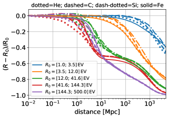
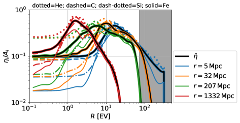
Figure 1: The impact of interactions with the CMB and the EBL on the CR properties: Left: The change of rigidity of different primary particle types as a function of the propagation distance. Right: The modification factor $\eta_{i}$ of different nucleus types (coloured lines) as well as their average (black solid line) for different source distances as a function of the rigidity for a source spectral index $\alpha\simeq 2$ and $\hat{R}=72\,\text{EV}$ (as indicated by the black shaded area).

As shown in the right panel of Fig. 1, $\eta_{i}$ in principle depends on the initial nucleus type $i$. However, at high rigidities and/or large source distances it converges towards $A_{i}$, corresponding to the total photo-disintegration of the initial nucleus of mass number $A_{i}$, modified by the exponential cutoff at the maximal rigidity. Although there is still some weak dependence on the nucleus type at rigidities $\lesssim 10\,\text{EV}$, we will subsequently use the approximation that

$$\eta_{i}(R,r)\simeq A_{i}\,\bar{\eta}(R,r)\equiv A_{i}\,\langle\eta_{i}(R,r)/A_{i}\rangle_{i}.$$ (2.15)

Furthermore, we adopt for the calculation of $\eta_{i}$ an equipartition of He, C, Si and Fe nuclei, which corresponds to a mean mass number $\bar{A}=25$ at a given rigidity. Note that the chosen spectral index $\alpha$ has a comparably small impact on the spread of $\eta_{i}(R,r)/A_{i}$ as function of the CR type $i$, and in general this spread becomes smaller with decreasing $\alpha$. As an example, we note that for $R=1\,\text{EV}$ and $r=100\,\text{Mpc}$ the difference of the relative spread $[\eta_{He}(R,r)/4-\eta_{Fe}(R,r)/56]/(\eta_{He}(R,r)/4)$ between $\alpha=2$ and $\alpha=1.5$ is about $0.1$, hence, much smaller than the relative difference between $\bar{\eta}$ and $\eta_{i}(R,r)/A_{i}$ in most cases. Since the general spectral behavior of $\eta_{i}(R,r)/A_{i}$ is quite similar for all nuclei types, the relative difference of the actual modification factor $\eta_{i}(R,r)/A_{i}$ between two sources that feature similar elemental abundances are typically much smaller than a factor of five.

Including the modification factor $\eta_{i}$, the CR density is determined as

$$n_{i}(R,r,t_{\rm act})=\frac{S_{0,i}(R)}{4\pi\,c\,r^{2}}\,\xi(R,r,t_{\rm act})\,A_{i}\,\bar{\eta}(R,r).$$ (2.16)

Note that this approximation does not include the increased length of the propagation distance due to the deflections by the EGMF or the change of the diffusion length $l_{D}$ with distance due to the change of rigidity. The effect of the latter is roughly taken into account by using the average enhancement factor

$$\bar{\xi}(R,r,t_{\rm act})\equiv\langle\xi(R_{0}(R,x),r,t_{\rm act})\rangle_{x}=\frac{1}{r}\int_{0}^{r}\mathrm{d}x\,\,\xi(R_{0}(R,x),r,t_{\rm act}).$$ (2.17)

A comparison with the enhancement factor (2.11) for the limiting rigidities of $R_{0}$ and $R$, respectively, shows that $\bar{\xi}\simeq\xi(R_{0}(R,r))\simeq\xi(R)$ is valid for a very large range of parameters, i.e. where $l_{\rm D}\,{}^{\gg}_{\ll}\,r$ or $t_{\rm act}c\lesssim r$, so that averaging has only a minor impact on the results (cf. the left panel of Fig. 2). In the case of small rigidities (blue lines) the change of rigidity is negligible, hence $R\simeq R_{0}$, and for large rigidities (green lines) $l_{\rm D}\gg r$ so that the argument of the exponential term in Eq. (2.11) vanishes. For CR rigidities $\gtrsim 6\,\text{EV}$, EGMF strengths of $B_{\rm rms}\lesssim 1\,\text{nG}$ and a coherence length of $1\,\text{Mpc}$, the right panel of Fig. 2 illustrates that UHECRs from sources up to a few hundreds of Mpc have a diffusive propagation delay which is negligible compared to their source distance. For a significantly stronger EGMF and/or lower CR rigidities, there is only a small range of source distances where the average propagation delay is significantly larger than the source distance but smaller than the maximal propagation distance, i.e. $r<\Delta r<t_{\rm act}c+r$. Hence, in most cases the majority of UHECRs have on average a propagation length quite close to their source distance, so that it is reasonable to neglect the additional propagation length at zeroth order. Note that this holds even stronger in the case of quasi-ballistic propagation, where $\Delta r\propto r$, which e.g. leads to a flattening of $\Delta r(R=5.6\,\text{EV})$ at about 30 Mpc.

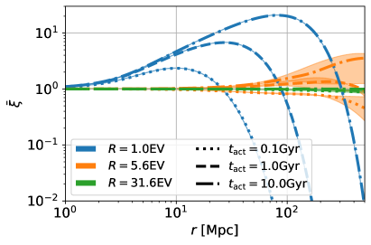
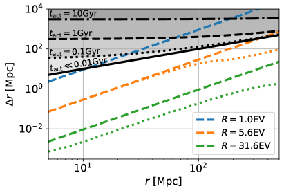
Figure 2: Left: The mean enhancement factor 2.17 as a function of the source distance for three different source lifetimes and rigidities. The edges of the coloured bands indicate the corresponding enhancement factor 2.11 for $R$ and $R_{0}(R,r)$, respectively. Right: The additional mean propagation length $\Delta r$ due to isotropic diffusion by the EGMF, where we use $B_{\rm rms}=1\,\text{nG}$ and $\lambda=1\,\text{Mpc}$. The dotted colored lines correspond to the resulting propagation delay for a rigidity $R_{0}(R,r)$ at the sources. The black lines indicate the maximal propagation length due to a finite source lifetime.

Finally, with $A_{i}\simeq 2\,Z_{i}$ the total CR density becomes

$$n(R,r,t_{\rm act})=\sum_{i}n_{i}(R,r,t_{\rm act})=n_{0}\,\left(\frac{R}{\check{R}}\right)^{-\alpha}\,\exp\left(-\frac{R}{\hat{R}}\right)\,\bar{\xi}(R,r,t_{\rm act})\,\bar{\eta}(R,r),$$ (2.18)

where

$$n_{0}=\frac{Q_{\rm cr}}{2\pi c\,r^{2}}\,\frac{\check{R}^{-\alpha}\,(2-\alpha)}{(\hat{R}^{2-\alpha}-\check{R}^{2-\alpha})}$$ (2.19)

does not depend on the initial nucleus type. Thus, we are able to compare our model predictions to observational data (see Sect. 3) without the need to specify the initial abundances of elements at the sources, which implies a substantial reduction of the dimensionality of the parameter space we have to consider.

2.2.1 Local radio galaxies

For a given total UHECR density (2.18) at a distance $r_{s}$ from an individual, local source $s$, the corresponding total UHECR intensity as function of rigidity is given by

$$J_{s}(R,r_{s},t_{\rm act})\equiv\frac{\mathrm{d}N_{\rm cr}}{\mathrm{d}R\,\mathrm{d}A\,\mathrm{d}t\,\mathrm{d}\Omega}=\frac{c}{4\pi}\,n(R,r_{s},t_{\rm act}),$$ (2.20)

if the intensity is isotropic. However, in all cases of interest for us, UHECRs do not propagate fully diffusively and thus we have to supply information on the angular dependence of the UHECR intensity. It has been shown in Ref. [67] that a Fisher distribution provides a good description of the angular distribution of the arrival directions of UHECRs after stochastic deflections in the EGMF. Hence, the resulting distribution of arrival directions $\theta_{\rm f}$ with respect to the source direction is computed from a random value $r_{\rm u}$ choosen from a uniform distribution over $[0,\,1)$ according to

$$\theta_{\rm f}=\arccos{\left\{1+\ln{\left(1-r_{\rm u}[1-\exp(-2\kappa)]\right)}/\kappa\right\}}.$$ (2.21)

From numerical simulations of UHECR sources with a finite lifetime the concentration parameter $\kappa$ that characterizes the Fisher distribution can be estimated by [39]

$$\kappa\simeq\frac{l_{\rm D}}{r_{s}}\,\left[2+\exp\left(-\frac{2r_{s}}{3l_{\rm D}}-\frac{1}{2}\left(\frac{r_{s}}{l_{\rm D}}\right)^{2}\right)\right]+\frac{0.44}{[ct_{\rm act}/r_{s}+1]^{0.8+0.4l_{\rm D}/(ct_{\rm act}+r_{s})}-1}.$$ (2.22)

As these simulations do not account for the change of rigidity we will subsequently use the average concentration parameter

$$\bar{\kappa}(R,r_{s},t_{\rm act})\equiv\langle\kappa(R_{0}(R,x),r_{s},t_{\rm act})\rangle_{x}=\frac{1}{r_{s}}\int_{0}^{r_{s}}\mathrm{d}x\,\,\kappa(R_{0}(R,x),r_{s},t_{\rm act}),$$ (2.23)

similar to the average enhancement factor (2.17) that is used to correct the absolute value of the flux. Here, the second term of Eq. (2.22) takes into account the finite lifetime of the source. The UHECR arrival maps that account for a turbulent and isotropic EGMF are subsequently determined using Eq. (2.21) for a given $\bar{\kappa}$ under consideration of the limited statistics of the most recent anisotropy study [68] of the Auger experiment. Moreover, we include the deflections by the JF12 Galactic magnetic field model using the so-called lensing technique, where anti-particles have been propagated backwards to obtain the trajectories of the regular particles that hit the Earth [69].

In case of high rigidities (see the green lines in the left panel of Fig. 3), where $l_{\rm D}\gg r_{s}$, the impact of the finite lifetime vanishes, since CRs propagate quasi-rectilinearly. In this case, we read from Fig. 3 that $\kappa\gg 10$ which corresponds to a mean deflection $\ll 23\degree$ with respect to the source direction. Hence, the change of rigidity can have a significant effect on $\kappa$. However, only at intermediate rigidities (see the orange lines in the left panel of Fig. 3), where $l_{\rm D}\sim r_{s}$ and $t_{\rm act}c\gtrsim r_{s}$, this leads to a significant change of the angular distribution of CR which corresponds to $0.1\lesssim\kappa\lesssim 10$. Now $\bar{\kappa}$ is typically close to $\kappa(R)$ indicating that the CR propagates most of its distance with a rigidity that is rather close to the observed one.

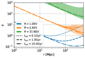
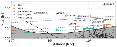
Figure 3: Left: The mean concentration parameter (2.23) as function of the source distance for three different source lifetimes and rigidities. The edges of the coloured bands indicate the corresponding concentration parameter (2.22) for $R$ and $R_{0}(R,r)$, respectively. Right: The radio flux of the considered source sample [70] (colored dots), as well as the dim sources (black dots and crosses) from the catalog of van Velzen et al. [71] that are (except for three close-by starburst galaxies) below the conservative source selection criterion [70] — as indicated by the black solid line. Above the black dotted line sources are likely able to provide a maximal rigidity $\hat{R}>1\,\text{EV}$ and above the colored dashed lines their CR flux is in case of pure rectilinear propagation at least $20\,\%$ (purple), $5\,\%$ (orange), or $2\,\%$ (green) of the brightest CR source in our sample (Cen A). The exact location of these constraints depends on several parameters. Here, the constraints are shown for an optimistic scenario using $\beta_{L}=0.89$, $g_{\rm m}=4/7$, $g_{\rm acc}=1$, and $k=0$.

For the choice of local radio galaxies included in our analysis, we use the catalogue defined in Ref. [70]. This catalogue is based on the source catalog of van Velzen et al. [71] which used the 2MRS catalog that selects sources by their infrared flux. In addition, it contains several powerful radio sources that have previously been missed by van Velzen et al. Moreover, only local sources up to 500 Mpc distance to Earth are considered, because at greater distances the UHECR flux is surpressed significantly, either by attenuation (via $\bar{\eta}$ at $R\gtrsim 10\,\text{EV}$) or by diffusion effects (via $\bar{\xi}$ at $R\lesssim 1\,\text{EV}$).

In addition, there is a low probability that sources at such large distances provide an individual flux contribution that is comparable to the one from nearby sources (as indicated by the dashed colored lines in the right panel of Fig. 3). On the other hand, those very nearby radio sources with a radio flux of a few Jy (which are predominantly starburst galaxies) can hardly provide the necessary energies (as indicated by the black dotted line in the right panel of Fig. 3). Thus, the complete local source sample consists of 39 sources, whereof only seven can be clearly identified as FR-II type. We have verified that only in the case of the compact object 3C 111 a moderate boosting is justified. For these seven FR-II sources dynamical evolution models provide a fairly accurate estimate on their jet power as well as their jet lifetime, which are shown in Table 1.

Table 1: Individual jet characteristics.

Source name	FR type	$Q_{\rm jet}$ [$10^{44}$ erg/s]	$t_{\rm act}$ [Myr]	Reference
3C 33	II	$2$	$61$	[72]
3C 98	II	$7$	$5.5$	[72]
3C 353	II	$2.3$	$22.1$	[72]
3C 390.3	II	$1.2$	$85$	[72]
3C 430	II	$0.68$	$23$	[a]
Pictor A	II	$2.4$	$61$	[a]
Cygnus A	II	$83$	$7$	[44, 73, 74], [a]
Centaurus A	I	$0.1$	$100$	[75, 76, 77, 78]

^[a] Private communication with Jerzy Machalski (calculations are based on their recent model [72]).

For the other sources, only in case of Centaurus A an individual assignment of its jet properties can be performed. However, even in this case these values are only an order of magnitude estimate. For the other sources, we apply the general radio-jet power correlation (2.1). The source lifetime $t_{\rm act}$ is treated as a free parameter for all FR-I sources except Centaurus A as well as in the case of those radio galaxies of unclear/other type with a radio brightness below $2\times 10^{25}\,\text{W}\,\text{Hz}^{-1}\,\text{sr}^{-1}$ at 151 MHz—which corresponds to the common transition power between FRs sources of type I and type II [79]. In the case of more powerful sources of unclear/other type we adopt the dynamical evolution model from Ref. [72] for FR-II sources and estimate the heuristic correlation function

$$t_{\rm lobe}=52\,\text{Myr}\,(Q_{\rm jet}/10^{44}\,\text{erg/s})^{-0.45}$$ (2.24)

between the jet power $Q_{\rm jet}$ and the age of the lobes $t_{\rm lobe}$ shown in Fig. 4.

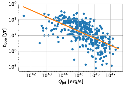
Figure 4: The lobe age of 361 FR-II sources dependent on their jet power (taken from [72]), as well as a heuristic correlation function as given by Eq. (2.24).

Individual sources can deviate from this correlation by more than an order of magnitude—in particular those that do not possess a typical FR-II morphology. Still, using this correlation is more justified than employing the same lifetime for all sources. Furthermore, it has also been confirmed by other observations [80] that the lower the jet power, the greater the chance of a long lifetime of high-luminosity radio galaxies. However, in case of low-luminosity radio galaxies (which have in their vast majority a FR-I morphology) this inverse correlation does not hold anymore as shown e.g. by Turner and Shabala [80]. Therefore we treat $t_{\rm act}$ as a single free parameter, common to all low-luminosity radio sources. For the others, i.e. the high-luminosity radio sources, we will subsequently suppose that their lifetime can be approximated by the age of their lobes, i.e. $t_{\rm act}\simeq t_{\rm lobe}$, either given in Table 1 or by Eq. (2.24).

2.3 UHECRs from the bulk of radio galaxies

In addition to the UHECRs from these bright, individual local radio galaxies, which we suppose to dominate the contribution on local scales, there is a diffuse contribution from the bulk of distant radio galaxies. Studies of the Local Supercluster indicate [81] that at redshift $\gtrsim 0.02$ inhomogenities in the large-scale distribution of the sources vanish and in case of a strong EGMF they will already be averaged out on smaller scales, so that we can assume this contribution to be isotropic. Moreover, these sources fill space nearly homogeneously with UHECRs, if the particles are able to propagate at least about the mean distance between the considered source class. According to the propagation theorem [82], the diffuse energy spectrum is independent of the particle propagation mode if the spatial separation between sources is smaller than all other characteristic length scales of propagation. Hence, we expect no modification of the diffuse spectrum by the EGMF and the enhancement factor $\bar{\xi}$ can be neglected.

Based on the radio luminosity function of low- and high-luminosity radio sources from Ref. [83], we use the so-called continuous source function (CSF)

$$\Psi_{0,i}(R,\,z)\equiv\frac{\mathrm{d}N_{\rm cr}(Z_{i})}{\mathrm{d}V\mathrm{d}R\,\mathrm{d}t}=\int S_{0,i}\big{(}R,\hat{R}(Q_{\rm cr})\big{)}\,\frac{\mathrm{d}N}{\mathrm{d}V\,\mathrm{d}Q_{\rm cr}}\,\mathrm{d}Q_{\rm cr}$$ (2.25)

following the approach of Refs. [41, 84]. Here, $\mathrm{d}N/(\mathrm{d}V\,\mathrm{d}Q_{\rm cr})$ is the number of radio sources per volume and luminosity, while $S_{0,i}(R,\hat{R}(Q_{\rm cr}))$ is the UHECR injection rate of a radio source with the maximal rigidity $\hat{R}(Q_{\rm cr})$. Using a sharp cutoff at $\hat{R}(Q_{\rm cr})$ instead of an exponential suppression, Eq. (2.25) can be solved analytically, for the solution see Eq. (3.17) in Ref. [41]. To account for the impact of the CMB and the EBL, we employ again the mean modification factor as given by

$$\bar{\eta}_{\rm csf}(R,z)=\langle\eta_{{\rm csf},i}(R,z)/A_{i}\rangle_{i}=\left\langle\frac{1}{A_{i}}\,\frac{\Psi_{i}(R,z)}{\Psi_{0,i}(R,z)}\right\rangle_{i}.$$ (2.26)

For the calculation of this function, we perform again a large set of 1D CRPropa simulations and compute the ratio $\Psi_{i}(R,z)/\Psi_{0,i}(R,z)$ of the attenuated and the unattenuated CSFs at a given redshift $z$. Because of the integration over the CR power $Q_{\rm cr}$, the modification factor $\bar{\eta}_{\rm csf}(R,z)$ depends not only on the assumed spectral index $\alpha$ but also on the parameters $g_{\rm acc}$, $g_{\rm m}$, $k$ and $\beta_{\rm L}$ that define the correlation between radio and CR power.

The deviations between $\eta_{{\rm csf},i}(R,z)/A_{i}$ for different nuclei are in general smaller than those shown in the right panel of Fig. 1, because of the larger source distances. The difference of $\bar{\eta}_{\rm csf}(R,z)$ between low- and high-luminosity radio sources shown in Fig. 5 exposes that the latter provide a larger amount of secondaries, as they are more numerous at high redshifts than low-luminosity radio sources and are in principle able to accelerate UHECRs to higher rigidities. The total contribution to the UHECR intensity by the bulk of radio galaxies between a redshift $\check{z}$ and $\hat{z}$ is given by

$$J_{\rm csf}(R,t_{\rm act})=\frac{c}{4\pi}\,\int_{\check{z}}^{\hat{z}}\mathrm{d}z\,\,\left|\frac{\mathrm{d}t}{\mathrm{d}z}\right|\sum_{i}\Psi_{0,i}(R,\,z)\,A_{i}\,\bar{\eta}_{\rm csf}(R,z)$$ (2.27)

with

$$\left|\frac{\mathrm{d}t}{\mathrm{d}z}\right|=\left[H_{0}\,(1+z)\,\sqrt{(1+z)^{3}\Omega_{\rm m}+\Omega_{\Lambda}}\right]^{-1}\,,$$ (2.28)

where we use the standard $\Lambda$CDM cosmology with a Hubble constant $H_{0}=70\,\text{km}\,\text{s}^{-1}\,\text{Mpc}^{-1}$, $\Omega_{\rm m}=0.3$, and $\Omega_{\Lambda}=0.7$. Furthermore, we obtain that $\sum_{i}A_{i}\Psi_{0,i}(R,\,z)\simeq 2\,\Psi_{0}(R,\,z)$, with $\Psi_{0}(R,\,z)$ as the total initial CSF, is again independent of the initial elemental abundances, since the mean charge number $\bar{Z}\equiv\sum_{i}f_{i}\,Z_{i}$ (that is used in Eq. (3.17) of Ref. [41]), where $f_{i}$ denotes the fractional abundances of a given element $i$, and $A_{i}\simeq 2\,Z_{i}$.

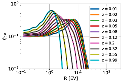
Figure 5: The average modification factor $\bar{\eta}_{\rm csf}$ for the bulk of low-luminosity (left) and high-luminosity (right) radio sources, respectively, with $\alpha=2$, $g_{\rm acc}=0.5$, $g_{\rm m}=0.6$, and $k=0.5$.

3 Results and comparison to data

The goal of this work is to investigate if a sample of individual local radio galaxies is sufficient to explain the mean features of the UHECR data, and to which amount a diffuse contribution by the bulk of radio galaxies is in addition needed. Further, if such a sample exists we try to identify the most relevant individual sources and their characteristics, in particular the lifetime of low-luminosity sources, their CR power and the maximal rigidity.

3.1 From rigidity to energy at Earth

To compare our model with data, the calculated UHECR intensity $J(R)$ needs to be converted into a function of energy. The total CR intensity $J_{R}=J_{\rm csf}+\sum_{s}J_{s}$ at Earth is composed of the sum of the diffuse flux from low- and high-luminosity radio galaxies as well as the local sample of radio-bright sources. For the latter we will investigate three different sub-samples (consisting of 5, 11 and 26 sources respectively), that are selected according to their CR flux based on the CR power $Q_{\rm CR}$ defined in Eq. (2.1) assuming rectilinear propagation (see the right panel of Fig. 3). Based on the supposed isotropy of the CSF contribution, we subsequently include only sources beyond the Local Supercluster, choosing $\check{z}=0.02$. However, our results hardly depend on this parameter choice because the bulk of radio galaxies at $z<0.02$ predominantly affects the total CSF contribution at high rigidities (above about 10 EV), where the individual local sources are expected to dominate the UHECR flux. At $z>1$ the CSF contribution above a few EV already vanishes, as can be seen in Fig. 5, so that without loss of generality we use $\hat{z}=1.5$ in the following. Since $J_{R}$ does not depend on the unknown initial elemental abundances at the sources, we avoid a multitude of additional free parameters. We convert the total rigidity spectrum at Earth into an energy spectrum using the observed mean logarithm of the mass number, $\langle\ln A\rangle_{\rm obs}$. In doing so, we do not account for the variance of the $\ln A$ distribution. This information could be used to constrain the initial CR composition at the sources, which is however beyond the scope of this work. Nevertheless, we like to stress that our approach does not rely on a pure composition at Earth, i.e. the $\langle\ln A\rangle_{\rm obs}$ contribution of the individual sources at Earth can differ, since either a single source or even multiple sources can contribute different CR nuclei at a given energy $E_{\rm obs}$ which in total sum up to the observed compositional data. Hence, we suppose that the observed rigidity can be estimated by $R_{\rm obs}(E,Z)=E_{\rm obs}/(eZ_{\rm obs})$, with $Z_{\rm obs}=\exp(\langle\ln A\rangle_{\rm obs})/2$. This is a good approximation for all nuclei except for protons which can be neglected in the energy range of interest for us. The conversion of the CR intensity from rigidity to energy is given by

$$J_{E}(E)=J_{R}(R)\,\biggl{|}\frac{\mathrm{d}R_{\rm obs}}{\mathrm{d}E_{\rm obs}}\biggl{|}=\frac{J_{R}(R)}{e}\,\left[\frac{1}{Z_{\rm obs}}-\frac{E_{\rm obs}}{Z_{\rm obs}^{2}}\,\frac{\mathrm{d}Z_{\rm obs}}{\mathrm{d}E_{\rm obs}}\right]\,,$$ (3.1)

and the corresponding standard deviation by

$$\Delta J_{E}(E)=\frac{J_{R}(R)}{e}\,\sqrt{\left[\frac{2E_{\rm obs}}{Z_{\rm obs}^{3}}\,\frac{\mathrm{d}Z_{\rm obs}}{\mathrm{d}E_{\rm obs}}-\frac{1}{Z_{\rm obs}^{2}}\right]^{2}\,(\Delta Z_{\rm obs})^{2}+\frac{E_{\rm obs}^{2}}{Z_{\rm obs}^{4}}\,\left(\Delta\frac{\mathrm{d}Z_{\rm obs}}{\mathrm{d}E_{\rm obs}}\right)^{2}}$$ (3.2)

with

$$\Delta Z_{\rm obs}=Z_{\rm obs}\,\Delta\langle\ln A\rangle_{\rm obs}\qquad\text{and}\qquad\Delta\frac{\mathrm{d}Z_{\rm obs}}{\mathrm{d}E_{\rm obs}}=Z_{\rm obs}\,\frac{\mathrm{d}\langle\ln A\rangle_{\rm obs}}{\mathrm{d}E_{\rm obs}}\,\Delta\langle\ln A\rangle_{\rm obs}\,.$$ (3.3)

This flux conversion demands a non-vanishing derivative $\mathrm{d}R_{\rm obs}/\mathrm{d}E_{\rm obs}$ and therefore we have to neglect the irregularities visible in the composition data shown in the left panel of Fig. 6. Determining $Z_{\rm obs}(E_{\rm obs})$ by a linear spline function between 2 EeV and 100 EeV yields a quite accurate description of the $\langle\ln A\rangle_{\rm obs}$ data, in particular at lower energies.

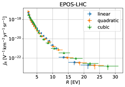
Figure 6: Using the composition data for the hadronic interaction model EPOS-LHC to convert rigidity into energy. Left: Inferred mean logarithmic mass of UHECRs $\langle\ln A\rangle_{\rm obs}$ as a function of energy as well as three different splines (polynomials of different degrees) that interpolate those data that is marked by an open square. In case of the linear spline (blue solid line) also the uncertainty range is shown. The greyed area marks the energy range that is not considered in our analysis. The inferred $\langle\ln A\rangle_{\rm obs}$ values are based on measurements of the depth of shower maximum with the Auger fluorescence detectors (FD) [4] and surface detectors (SD) [85]. Right: The conversion of the Auger flux $J_{E}$ into $J_{R}$ using the different splines of $\langle\ln A\rangle_{\rm obs}$ that are illustrated in the left panel.

The fit using a higher order polynomial shown in addition does not provide a significantly better approximation of the composition data. Nevertheless, a change of the fit function will lead to minor changes in $R_{\rm obs}$ as well as $J_{E}$. To illustrate these differences, we use the observed energy spectrum $J_{E}$ and apply Eq. (3.1) to convert it into the rigidity spectrum $J_{R}$ shown in the right panel of Fig. 6. Clearly, the resulting rigidity spectrum depends on the composition data and their accuracy, what is, however, a general issue for every approach that tries to explain the UHECR data. Characterizing UHECRs from their sources to Earth only by their rigidity provides the benefit that we can use the rather well-known composition data at Earth to split the rigidity information into energy and charge/mass number, instead of introducing an arbitrary source composition in the first place. Thus, our fitting approach ensures a priori that the $\langle\ln A\rangle_{\rm obs}$ data are described with high precision according to the linear spline shown in the left panel of Fig. 6. At high energies, we include the composition data obtained with the Auger surface detectors [85], to obtain a better constraint on $Z_{\rm obs}$ at and beyond the last data point derived from the fluorescence detector data [4]. Unfortunately, these data indicate opposite trends.

Unless otherwise stated, we will use the $\langle\ln A\rangle_{\rm obs}$ prediction based on the hadronic interaction model EPOS-LHC [86, 87], as the resulting mean mass numbers are in-between those from the two alternative interaction models QGSJet II-04 [88, 89] and Sibyll2.3c [90].

3.2 Fit parameters and procedure

In what follows, we will compare our model to the observed dipole characteristics, i.e. its strength and direction [68], as well as the energy spectrum [2] above $5\,\text{EeV}$ from the Pierre Auger Observatory. We apply a so-called Galactic lens (more details on the lens and its generation can be found in Ref. [69, 91]) based on the JF12 model to account for the CR deflections by the GMF. Dependent on the rigidity of each UHECR and its arrival direction, the JF12 field leads to deflections up to several tens of degrees of the average arrival direction at Earth with respect to the source direction. The main challenge in a comparison with the UHECR data results from the large number of dimensions of the parameter space of our model shown in Table 2. It contains the source parameters $g_{\rm m}$ and $k$ defining the conversion from jet into CR power, the acceleration efficiency $g_{\rm acc}$ that sets the maximal rigidity and the source spectral index $\alpha$ which depends on the details of the acceleration process. Except for $\alpha$, all these parameters are constrained only within an order of magnitude. In the case of acceleration by a non-relativistic, strong shock in the outer jet, as induced e.g. by its backflows [55], we expect only minor deviations from the canonical value of $\alpha=2$ leading to $1.5\lesssim\alpha\lesssim 2.5$, caused by non-linear effects [92, 93]. Different acceleration mechanisms including shear acceleration in the large-scale jet [56, 94], are expected to lead to smaller values of $\alpha$ and may accelerate particles to ultra-high energies in (trans-) relativistic jets. In addition, we only got some rough constraints on the lifetime of low-luminosity radio sources [80], $1\,\text{Myr}\lesssim t_{\rm act}\lesssim 1\,\text{Gyr}$, as well as the strength of the EGMF [95] $B_{\rm rms}\lesssim 2\,\text{nG}$ supposing 1 Mpc as coherence length. In addition, most of these parameters—in particular $g_{\rm m}$, $k$, $g_{\rm acc}$, and $t_{\rm act}$—are expected to vary from source to source, because of differences in the details of their power supply or their evolutionary stage. Thus, we likely end up with an underdetermined, non-linear system that needs to be solved.

Due to limited computational resources, we will only differentiate $g_{\rm m}$ and $g_{\rm acc}$ between the sources: These two parameters impact mainly the spectral relevance of these sources and can incorporate partly the uncertainty from the radio-jet power correlation. Finally, we quantify the goodness of the fit by the chi-squared value $\chi^{2}(k,\,t_{\rm act},\,B_{\rm rms})=\sum_{j}(P_{j}-O_{j})^{2}/\sigma^{2}(P_{j},O_{j})$, where $P_{j}$ ($O_{j}$) denotes the model prediction (observation) of the total diffuse flux as well as the dipole strength and direction at a given energy. Finally, we use an optimization routine to obtain the global minimum of the multivariate chi-squared function for a given parameter combination of $(k,\,t_{\rm act},\,B_{\rm rms})$. Hence, the parameter optimization is only performed using $g_{\rm m}$, $g_{\rm acc}$ and $\alpha$—which yields in the case of five individual, local sources (plus the bulk of low- and high-luminosity radio galaxies) already $15=5\times 2+2\times 2+1$ parameters that need to be determined within the given constraints. However, we manage to slightly minimize the parameter space of the optimization algorithm by using a linear least-squares problem solver to compute $g_{\rm m}$ (see the Appendix A for more details). Table 2 summarizes all details on the free (first three rows) and fixed (last five rows) model parameters used in the fit procedure.

Table 2: Model parameters. The first three rows give the range of the free parameters, while the rest of the parameters are fixed to the quoted values.

Parameter	Value(s)	Per Source	Description
$g_{\rm m}$	$[0.001,\dots,\,0.9]$	yes	matter-to-jet power ratio
$g_{\rm acc}$	$[0.001,\dots,\,1]$	yes	acceleration efficiency
$\alpha$	$[1.5,\dots,\,2.5]$	no	source spectral index
$k$	$[0.1,\,0.5,\,1,\,5]$	no	leptonic-to-hadronic energy density ratio
$t_{\rm act}$ [Gyr]	$[0.01,\,0.05,\,0.1,\,0.5,\,1,\,5,\,10]$	no	low luminosity source lifetime
$B_{\rm rms}$ [nG]	$[0.1,\,0.5,\,1,\,5]$	no	rms EGMF strength
$l_{\rm c}$ [Mpc]	1	no	EGMF coherence length
$\check{R}$ [GV]	1	no	minimal CR rigidity
$\beta_{L}$	0.89	no	radio–jet power correlation index
$\check{z}$	0.02	no	minimal CSF redshift
$\hat{z}$	1.5	no	maximal CSF redshift

In general, it is quite likely that not only $g_{\rm m}$ and $g_{\rm acc}$, but also $t_{\rm act}$, $\alpha$, and $B_{\rm rms}$ vary (at least slightly) between the sources so that the following fit results will certainly improve by an expansion of the considered parameter space. Although, this does not necessarily involve an improved reduced chi-squared result—including the increased number of degrees of freedom. Further, it is not the goal of this work to identify the particular best fit scenario, as this certainly requires more precise data with respect to the Galactic and extragalactic magnetic fields, the source physics as well as the UHECR measurements. However, we verified for an individual assignment of $\alpha$ in case of a small local source sample, that the $\chi^{2}$ results only improve on average by a factor of about 0.9 with no changes on the general outcome, that is shown in the following.

3.3 Fit results

The $\chi^{2}$ results for our fit procedure are shown in the upper panel of Fig. 7 for a local source sample consisting of the five brightest CR sources: Centaurus A, Centaurus B, Virgo A, Fornax A, and Cygnus A (this smallest sample is subsequently referred to as S5). With such a small local source sample, the resulting distribution of chi-squared values exposes that a strong EGMF is needed as well as a rather long lifetime ($\gtrsim 1\,\text{Gyr}$) of Fornax A and Virgo A. Including the residuals with respect to the quadrupole data, this preference becomes stronger without significantly changing the following outcome: First, only Virgo A and Fornax A yield a significant contribution of at least $\sim\text{few}\times 10\%$ to the observed UHECR intensity. Second, the UHECR data are already explained quite well, apart from the right ascension of the dipole direction below $32\,\text{EeV}$, which shows deviations of up to $35\degree$. The assumed leptonic-to-hadronic energy ratio $k$ has only a minor impact on the fit. The comparison of the different sized local source samples shows that there is some benefit in increasing S5 by Pictor A, Hydra A, 3C 270, PKS 1610-60, 3C 353, and PKS 2153-69 (hereafter S11). Adding even more sources does not yield a significant improvement of the resulting $\chi^{2}$ values. However, based on the location of these local sources in the sky (see Fig. 8) we do not expect that the small source samples (S5 or S11) will be able to explain the recent indications of medium-scale anisotropy [96, 97], this issue will be discussed in see Sect. 5. Moreover, the optimization algorithm only accounts for the dipole anisotropy which is the most robust directional information that we currently have. The inclusion of higher order anisotropies, for which no firm detection exists, would lead to a significantly higher computational effort.

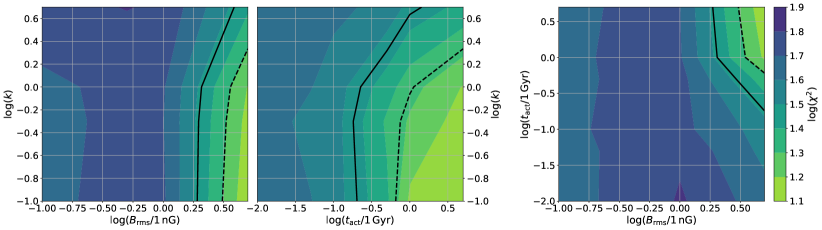
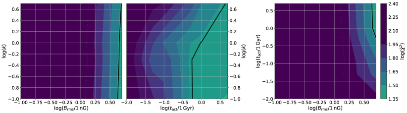
Figure 7: The marginalised (over the third parameter) chi-squared distribution that results from the optimization routine (upper panel) as well as after including the residuals by the quadrupole data (lower panel). Here the local source sample S5 is used. The black lines correspond to a chi-squared value of $20$ (dashed) and $30$ (solid), respectively.

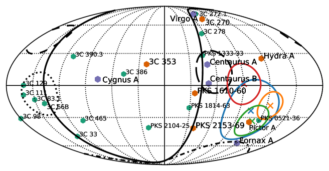
Figure 8: Our sample of radio galaxies shown in Galactic coordinates: The S5 sample (purple hexagons), the additional S11 sources (orange hexagons), and the additional S26 sources (green hexagons). Colored crosses (and surrounding lines) give the observed dipole direction (and uncertainty) at $[4,\,8]\,$ EeV (blue), $[8,\,16]\,$ EeV (yellow), $[16,\,32]\,$ EeV (green), $>32\,$ EeV (red). The black dashed and dash-dotted lines refer to the three most visible excesses of CR flux above 40 EeV in 2019 as taken from [96] and the black dotted line shows the approximate location of the excess that emerged recently [97]. The black solid line indicates the Supergalactic plane.

3.3.1 Eleven local sources

Using the source sample S11 consisting of eleven sources as well as the diffuse contribution from low- and high-luminosity radio galaxies, the upper panel of Fig. 9 shows that the parameter space of $(k,\,t_{\rm act},\,B_{\rm rms})$ is hardly constrained by the data, with the exception of preferring a rather small leptonic energy density ($k<1$) of these sources. Since it is not possible to single out a best-fit in the $(k,\,t_{\rm act},\,B_{\rm rms})$ space, we account in addition for the quadrupole anisotropy in the post analysis: Keeping the fixed parameters given by the optimization routine, we add the residuals of the quadrupole data, obtaining an enhanced chi-squared value $\tilde{\chi}^{2}$. Here we only account for the averaged quadrupole amplitude $Q=\sqrt{\sum_{ij}Q_{ij}^{2}/9}$. Note that the observed quadrupolar components are currently not significant in any of the considered energy bins, so that the actual quadrupole strength might also be significantly smaller than what is used in the following. As shown in the lower panel of Fig. 9, the inclusion of the averaged quadrupole amplitude yields a preference for long lifetimes of low-luminosity sources as well as a large EGMF strengths, emphasizing the importance of the quadrupole data in case of a larger local source sample. Strong EGMF fields combined with short source lifetimes are strongly disfavoured, with $\chi^{2}\gtrsim 100$.

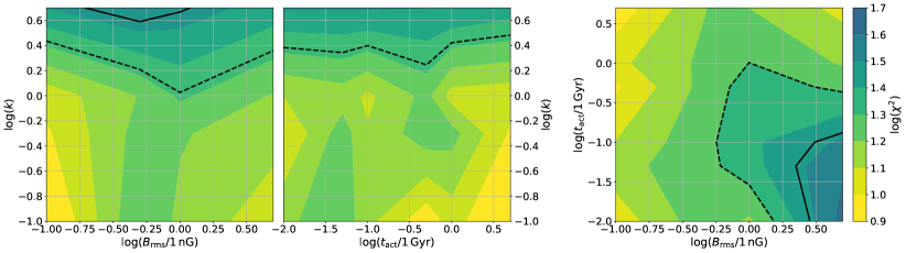
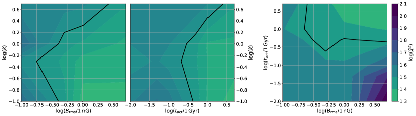
Figure 9: The marginalised (over the third parameter) chi-squared distribution that results from the optimization routine (upper panel) as well as after including the residuals by the quadrupole data (lower panel). Here the local source sample S11 is used. The black lines correspond to a chi-squared value of $20$ (dashed) and $30$ (solid), respectively.

Even including the quadrupole data, there is a multitude of scenarios allowed. Investigating the relative contribution of the different sources requiring an acceptable agreement with the data (selected by $\tilde{\chi}^{2}<30$), we recognize the following (see Fig. 10):

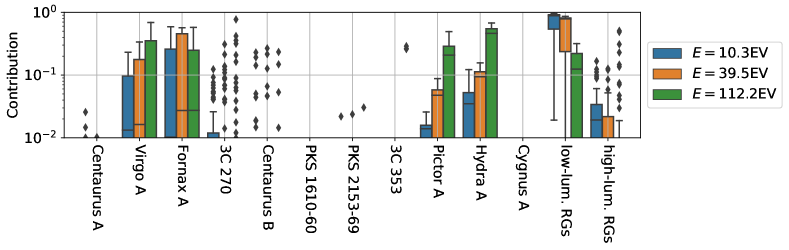
Figure 10: The relative contribution of the different sources to the UHECR flux at three different energies. Only results with $\tilde{\chi}^{2}<30$ are included. The solid line within the boxes refers to the median, the box represents the interquartile range (difference between the 75th and 25th percentiles of the data), the minimal and maximal values (excluding outliers) are indicated by the error bars, and outliers are shown as diamonds.

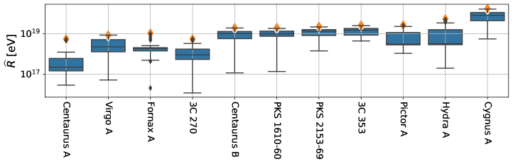
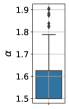
Figure 11: The distribution of the CR power (upper panel) and the maximal rigidity (lower left panel) of individual radio galaxies of the local source sample S11 as well as the distribution of the source spectral index (lower right panel). Only results with $\tilde{\chi}^{2}<30$ are included. The orange triangle in the upper panel indicates the underlying jet power $Q_{\rm jet}$, and the orange diamond in the lower panel gives the parameter independent rigidity $\sqrt{Q_{\rm jet}/c}$. Details on the boxplot features are given in the caption of Fig. 10.

On average, the diffuse contribution of low-luminosity sources dominates at most energies, in particular at $E\ll 100\,\text{EeV}$, while the majority of the local sources in the S11 sample contribute less than $1\,\%$. Surprisingly, also Centaurus A contributes only a negligible fraction to the total UHECR intensity, especially at high energies, while the most significant local sources on average are Virgo A, Fornax A, Pictor A, and Hydra A. The latter two are important in particular at the highest energies, $E\sim 100\,\text{EeV}$. The relative dominance between those four sources depends significantly on the EGMF strength and their lifetimes. There are however other scenarios where sources such as 3C 270, Centaurus B or 3C 353 contribute a significant percentage of the UHECR flux, as visible in the Fig. 10 or the upper panel of Fig. 12. The best-fit scenarios also exclude a major contribution of several local sources, such as Centaurus A (especially at high energies) and Cygnus A (especially at low energies)—what mostly results from their extreme distances to Earth (as well as the relative short lifetime in case of Cygnus A) as further elaborated in Sect. 4. Figure 11 displays the mean and spread of the main source characteristics (CR power, maximal rigidity, spectral index) of the fits with $\tilde{\chi}^{2}<30$ for the S11 sample. On average, their CR power is about an order of magnitude smaller than the given jet power, and the maximal rigidity is mostly smaller by factor of about two to five than $\sqrt{Q_{\rm jet}/c}$, An exception is Centaurus A, whose median maximal rigidity is the smallest of all local sources. Note that the reference value of the individual jet power depends for most sources (exceptions are Centaurus A, Cygnus A, Pictor A and 3C 353) on the supposed radio-jet-power correlation [45]. Further, we obtain a clear indication of a hard source spectrum of $\alpha\sim 1.5$, which has already been the case for the S5 results. The preference for rather hard spectra is in line with previous results which used an “average source” approach [98, 99]. Allowing for an even harder source spectrum the optimization procedure will also deliver a harder source spectrum on average, however, the corresponding chi-squared-values improve only marginally. Hence, our fit results are not very sensitive to the choice of $\alpha$, and we could fix $\alpha$ at some value in the range $1\lesssim\alpha\leq 2$ without introducing any major differences in the outcome.

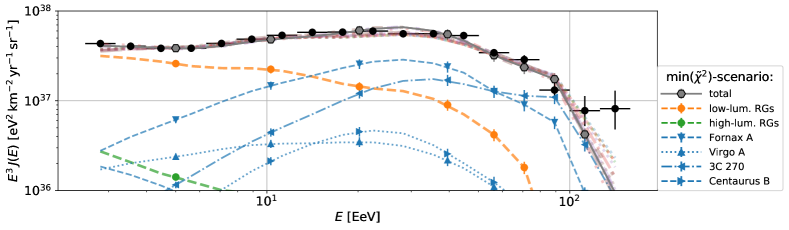
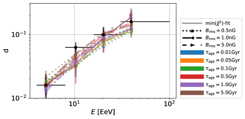
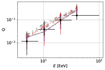
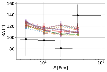
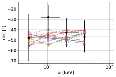
Figure 12: The best-fit model predictions using the S11 local source sample and the corresponding observational data (black markers) of the energy spectrum [2] and the anisotropy characteristics [68], respectively. Upper panel: The resulting energy spectrum for the scenario with the smallest $\tilde{\chi}^{2}$ value including its different contributions as well as the total spectra for all scenarios yielding $\tilde{\chi}^{2}<30$ (dimmed colored lines without markers). The markers of the model prediction indicate those energies that have been taken into account in the in the chi-squared calculation. Middle panel: The resulting dipole (left) and quadrupole (right) amplitude for all scenarios with $\tilde{\chi}^{2}<30$ (right). Lower panel: The corresponding dipole direction in right ascension (left) and declination (right) of the different scenarios.

Looking at the corresponding fits to the data in Fig. 12, we recognize that our model yields for almost all (accepted) scenarios a fairly accurate description of the intensity spectrum, even at energies below the ankle which are outside our fit range. In addition, the energy dependence of the dipole and quadrupole strength is reproduced well, where one should keep in mind again that the latter has not even been accounted for by the optimization routine. The clearest disagreement emerges from the dipole direction as our local source sample can hardly account for those strong non-monotonous changes, such as for the right ascension above $32\,\text{EeV}$ or the declination between 8 and 16 EeV, that are indicated by the data. Further, there is a systematic difference of about 20$\degree$ in right ascension between the observed dipole and our predictions. However, in most cases we are still within or at most a few degrees off the uncertainty range of the observations (for a more detailed discussion on this issue see Sect. 4).

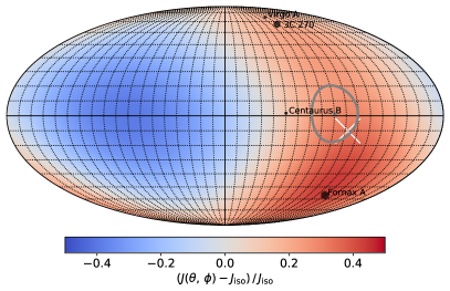
Figure 13: Mollweide projection in Galactic coordinates of the UHECR arrival directions at 40 EeV averaged on top-hat windows of $45\degree$ radius. Shown is the min($\tilde{\chi}^{2}$)-scenario based on the S11 local source sample before (left) and after (right) propagation through the Galactic magnetic field. The white cross shows the resulting dipole direction, whereas the observed dipole direction and its uncertainty at about this energy ($>32\,\text{EeV}$) is indicated by the grey cross and the surrounding solid line. Sources that provide more than $10\%$ of the flux at this energy are indicated by black hexagons (their size scales with the source contribution).

We can conclude that a local source sample consisting of either Hydra A and Pictor A or Virgo A/ 3C 270 and Fornax A is sufficient to explain the data. Hence, the local source sample can in principle be reduced to a combination of these two sources without a significant change in the goodness of the fit. But, it needs to be emphasized that such a scenario requires an EGMF strength at the order of nG (for 1 Mpc coherence length) as well as a long lifetime of about Gyrs or more. Analysing the angular distribution of the arriving CRs at the highest energies (see Fig. 13) it becomes clear that these fit scenarios lead to a flux deficit at about the whole hemisphere at low Galactic latitudes ($l\lesssim 180\degree$). Further, we illustrate the impact of the Galactic magnetic field, which shifts the dipole direction by about $10\,\degree$ in case of this particular scenario. Next, we will test if a substantial increase of the local source sample of up to 26 sources (hereafter S26), including several sources at a Galactic longitude $l\sim 150\degree$ close to the Galactic plane, introduces some substantial changes to the previous outcome.

3.3.2 Twenty-six local sources

Although the goodness of the fit does not improve significantly by doubling the size of the local source sample, the use of the S26 sample introduces some major differences with respect to the previous results: There are several fits with $\tilde{\chi}^{2}<30$ for a short source lifetime, $t_{\rm act}\sim 10\,\text{Myr}$, and there is much more variety in the contribution by the different sources: First, there are still several scenarios (for $B_{\rm rms}\sim 1\,\text{nG}$ and $t_{\rm act}\sim 1\,\text{Gyr}$) that suggest that Fornax A and Virgo A are the dominating sources. However, in addition a minor contribution on the order of about 10% at 40 EeV by sources such as 3C 98, PKS 1333-33, 3C 129 or 3C 111 is introduced. Second, we obtain multiple scenarios, where there is no need for a contribution by Fornax A and Virgo A. In these cases, typically some combination of the local sources Hydra A, Centaurus B, 3C 98, 3C 270, Pictor A and PKS 1333-33 can explain the data. Figure. 14 gives an illustrative examples of the CR arrival directions at 40 EeV for such a scenario with and without the impact of Galactic magnetic field deflections.

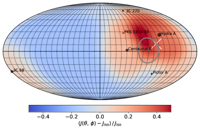
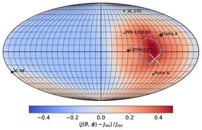
Figure 14: Mollweide projection of UHECR arrival directions at 40 EeV in Galactic coordinates averaged on top-hat windows of $45\degree$ radius. Shown is the best-fit scenario based on the S26 local source sample for $B_{\rm rms}\simeq 1\,\text{nG}$, $t_{\rm act}\simeq 10\,\text{Myr}$ and $k=1$ before (left) and after (right) propagation through the Galactic magnetic field. Markers and lines refer to the same properties as given in Fig. 13.

In addition, the use of the S26 source sample leads to some improvement of the resulting anisotropy features, in particular the right ascension of the dipole direction due to the contributions of 3C 129 and/or 3C 98, as can be seen in Fig. 15. In general, the increase of the local source sample allows for a stronger energy dependence of the dipole direction, but the agreement with the observed declination of the dipole direction between 8 and 16 EeV is still not perfect.

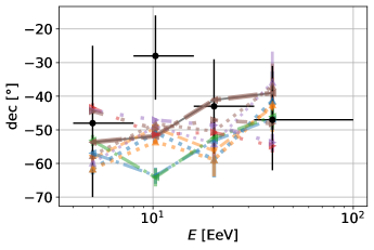
Figure 15: The best-fit results of the dipole direction in right ascension (left) and declination (right) using the S26 local source sample.

4 Discussion

Based on the individual properties of local radio galaxies, we have developed a model for their possible UHECR contribution at Earth. In the following, we discuss first the main assumptions we have used:

1. Magnetic field: The most significant influence on our outcome results from the impact of the EGMF and the GMF on the CR propagation. The chosen uniform and isotropic turbulent EGMF does not introduce any systematic shift of the UHECR arrival directions, but only spreads the angular distribution. We have adopted this simplified approach since EGMF models based on magnetohydrodynamics simulations differ strongly in their predictions [100]. Furthermore, the structure of a possible regular component which may shift the UHECR arrival directions in particular from sources in the Supergalactic plane, cannot be predicted by such simulations. In addition, the effective field strength of the EGMF will depend on the source location, such that CRs from sources within the Supergalactic plane have to cope with a significantly higher field strength than those that originate outside the plane. However, using a non-uniform EGMF model also leads to the ambiguity of the exact source location within this magnetic field structure causing an additional source of uncertainty. Including such a non-uniform, turbulent field could change the dipole direction and lead to some additional contribution, e.g. by rather distant sources outside the Supergalactic plane, such as Cygnus A or 3C 353, that feature short lifetimes. But in general, the current (and most likely future) lack of information on the EGMF will always yield the major source of uncertainty with respect to any kind of UHECR source prediction.
   In contrast to the used EGMF, the GMF has a significant effect on the dipole direction due to its regular field component. While the used JF12 model is the most sophisticated attempt to model the GMF, it is built on a limited set of information and has several weaknesses [101, 102]. Therefore the shift of the dipole direction predicted in the JF12 model has a rather large systematic error which we have not included in our fit procedure.

2. Mean modification factor: The impact of CR interactions with photons from the CMB and the EBL are incorporated by calculating the ratio of the modified and the unmodified spectral rigidity distribution for a given set of parameters. The modified distribution is obtained from 1D simulations, hence without including the increased travel time of CRs caused by magnetic field deflections. Further, we only account for the elemental mean of this factor to become independent of the unknown source abundances of different CR elements. This approach yields a significant reduction of the parameter space we have to evaluate but introduces uncertainties up to about a factor of five for small source distances and rigidities (cf. with the right panel of Fig. 1). Thus, the closer the individual radio galaxy, the higher is the chance of an additional modification of its flux contribution at rigidities $<10\,\text{EV}$, whereas at the highest rigidities the mean modification factor $\bar{\eta}$ is fairly accurate.

3. Elemental composition of UHECRs at Earth: Using the mean modification factor allowed us to determine the rigidity dependent UHECR intensity $J_{R}$ at Earth independent of the initial source abundances. To compare our prediction with the observations, we have converted $J_{R}$ into the energy space by using the observed composition data for $\langle\ln A\rangle_{\rm obs}$. For the considered energies above 4 EeV, where protons are mostly absent, it is appropriate to use $Z\simeq A/2$. Since our model predictions only depends on the CR rigidity, there is no need to include the information on the variance of the observed composition as we still have the freedom to choose, e.g., different CR mass numbers from different sources at the same energy, keeping $\langle\ln A\rangle$ fixes.

4. Source model: We have determined the jet power and lifetime of individual high-luminosity radio galaxies from a recent dynamical evolution model [72], whereas the jet power of the other sources (except for Centaurus A) has been estimated from the well-established correlation between radio and jet-power [45]. Although this correlation holds predominantly for FR-II sources, observations indicate a similar correlation for low-luminosity sources [44]. The rather large uncertainties and deviations from the given correlation for individual low-luminosity radio galaxies is partly compensated by allowing for an individual value of the fraction $g_{\rm m}$ of jet and matter power. Similarly, this parameter can on average also account for a possible enhanced activity of the individual sources in the past, such as indicated for Centaurus A [77, 76] and Fornax A [103].

Based on this model, we are able to predict the anisotropic UHECR intensity as a sum of contributions from individual local radio sources plus the isotropic contribution from low- and high-luminosity radio galaxies. A good agreement with the observational data—including the energy spectrum below the ankle as well as the quadrupole strength which where both not included in the fitting procedure—is already obtained by using only Fornax A as well as Virgo A and/or 3C 270 as local sources. However, in this scenario the EGMF strength has to be around $B_{\rm rms}\sim 1\,\text{nG}$ (for a coherence length of 1 Mpc), while the lifetimes of the sources have to be very large, of the order of Gyrs. In these cases, the ankle of the CR spectrum often marks the transition from a dominant contribution by the bulk of low-luminosity radio galaxy (at $E\lesssim 5\,\text{EeV}$) towards the dominance by local sources (at $E\gtrsim 5\,\text{EeV}$). The diffuse contribution by high-luminosity radio sources is on average at a level of a few percent at most.

Including more local sources—in particular at Galactic longitudes between 90° and 180°—leads to a multitude of possible scenarios where, e.g., Hydra A, Pictor A or Centaurus B can become the dominating UHECR sources without improving the fit significantly. Hence, data on the large-scale anisotropy of UHECRs alone do not allow one to single out a specific set of dominant local source of CRs. However, our analysis shows that at least one of the previously mentioned sources will have a major impact on the UHECR data, if radio galaxies are the sources of UHECRs. We could also exclude a major UHECR contribution from plenty of local sources: Perhaps most surprisingly Centaurus A and Cygnus A are among these disfavoured sources. The latter shows a quite short jet lifetime, leading to a strong suppression at low energies due to the deflections by the EGMF. Centaurus A on the other hand is rather the opposite case, being very close and showing a comparatively low CR power. Therefore a strong CR anisotropy is introduced by this source even for the strongest EGMF cases which can hardly be compensated by other local sources without generating a strong quadrupole anisotropy.

Our predicitions, as those of all other models aiming to explain the UHECR compositional data, depend on the hadronic interaction model applied to interpret the $X_{\rm max}$ data on the depth of the shower maximum. We decided to present the results in Sect. 3 for the interaction model EPOS-LHC, which yields in general the best agreements to the data—with a minimal chi-squared values of $\text{min}(\chi^{2})\sim 10$, whereas the other interaction models typically lead to scenarios with $\text{min}(\chi^{2})\sim 20$. The main differences in our results caused by using Sibyll2.3c or QGSJetII-04 can be summarized as follows:

Using the heavier chemical composition predicted by Sibyll2.3c yields quite similar results as previously discussed except for the following major differences: (i) Centaurus A (and B) can contribute a significant fracion of the observed UHECR intensity (especially at low energies), due to the stronger magnetic field deflections of nuclei with higher charges; (ii) the bulk of high-luminosity radio galaxies is on average more important than the low-luminosity counterpart; and (iii) the source spectrum is on average rather close to $\alpha\sim 2$. The major disagreement with respect to the data is the right ascension of the dipole direction below 32 EeV, which shows deviations of up to $55\degree$ using S5.

Using the lighter chemical composition prediction of QGSJetII-04 the UHECRs suffer from significantly less deflections by the EGMF and the GMF. Therefore the diffuse contribution by the bulk of low-luminosity radio galaxies becomes the major UHECR sources at all energies, while the main local sources (Fornax A and Hydra A) only contribute $10\%$ at most. Further, we obtain the need for a small leptonic-to-hadronic energy ratio, i.e. $k<1$, and a hard source spectrum. In this case, the major disagreement with respect to the data is either a too weak dipole strength above 16 EeV or a deviation of the dipole’s declination angle of up to $40\degree$ above 8 EeV. In addition, the inclusion of a larger number of local sources often leads to too large a quadrupole anisotropy, although the fit to the other data clearly benefits (leading to $\text{min}(\chi^{2})\sim 10$) from using S26 instead of the smaller source samples.

Next, we want to compare our results with four indications for medium-scale anisotropies at energies $\geq 40\,\text{EeV}$ [97, 96]. Two of these potential excesses at about ($12^{\rm h}\,50^{\rm m}$, -50°) and ($1^{\rm h}\,50^{\rm m}$, -35°) in equatorial coordinates are shown by black long-dashed and dash-dotted lines in Fig. 8, respectively. We find for several scenarios, such as the one with the smallest $\tilde{\chi}^{2}$ value, where Fornax A as well as Virgo A and/or 3C 270 are the dominating local sources a quite good agreement with theses excesses. However, the significance of these excess has declined [97]. Instead, another excess at about ($2^{\rm h}\,30^{\rm m}$, +50°) in equatorial coordinates (black dotted line in Fig. 8) has emerged that requires sources close to the Galactic plane at a Galactic longitude between $90\degree$ and $180\degree$. Although the S26 sample features at least four low-luminosity sources (3C 129, 3C 111, 3C 83.1 and 3C 66B) in this region—whereof 3C 111 shows even some evidence of boosted emission [104]—their possible contribution to this excess depends strongly on the GMF model and the rigidity of the particles at the highest energies. Using the JF12 model as well as a rather heavy chemical composition (according to the hadronic interaction models EPOS-LHC or Sibyll2.3c) above 40 EeV, UHECRs from these sources are deflected by more than $30\degree$ towards smaller Galactic latitudes, as can be seen for 3C 98 in Fig. 14. In the directions of the fourth excess of events at about ($9^{\rm h}\,30^{\rm m}$, +54°) shown by the short-dashed line in Fig. 8, our sample contains a deficit of sources, with 3C 390.3 as the closest possible source candidate. This deficit is not a result of our selection criteria but rather a general property of the distribution of radio galaxies, that shows a lack of sources at Supergalactic longitudes between 0°and 90° [81]. Despite this deficit it is known since several decades [105] that radio galaxies tend to be close to the Supergalactic plane—such as the hints for excesses in the UHECR data—whereas ordinary galaxies are more isotropically distributed. Finally, we note that the rather strong EGMF expected in the Supergalactic plane allows for a scenario where some of the actual source of UHECRs are no longer visible in the radio or even electromagnetic spectrum because of their finite lifetime but the majority of its delayed CRs are still arriving. This provides a possible but speculative scenario for the excess at about ($9^{\rm h}\,30^{\rm m}$, +54°) in particular.

5 Conclusions

We have examined if the stringent constraints imposed by the dipole and quadropole anisotropies as well as the UHECR spectrum and composition can be satisified by radio galaxies as UHECR sources. We have modeled 37 individual radio galaxies, constraining their properties using information from the radio-CR correlation and a dynamical evolution model. In addition, we have included the diffuse flux emitted by the bulk of non-local radio galaxies based on their radio luminosity distribution. Our approach of using a rigidity dependent injection rate reduced the number of independent parameters considerably and allowed us to fit the parameters $g_{\rm m}$ and $g_{\rm acc}$ individually for each source. Moreover, the CR propagation accounts for deflections by a turbulent EGMF as well as the GMF model by JF12.

The observed dipole anisotropy imposes a non-trivial constraint on the distribution of local UHECR sources. In the case of radio galaxies, there is a significant over-fluctuation of these bright sources at high Galactic longitudes ($l\gtrsim 240\degree$), which is roughly aligned with the observed UHECR dipole. Radio galaxies could have been ruled out as the major UHECR source had this distribution been flipped by $\sim 180\degree$ in longitude. In general, we have obtained a good description of the UHECR spectrum, its composition and the dipole and quadrupole anisotropies, even using only a small sample of the most powerful local sources combined with an isotropic contribution from low-luminosity radio galaxies. In particular, we find that scenarios where a few local sources—among them for instance Fornax A, Virgo A, 3C 270, Centaurus B or Hydra A—dominate the flux above the ankle, while low-luminosity radio galaxies contribute an isotropic background dominating below the ankle, provide a good fit to the data. Moreover, we found that neither the closest (Centaurus A) nor the most powerful source (Cygnus A) in the radio band is likely to give a dominant contribution to the observed UHECR events. Even though our results favor a major contribution by Fornax A as well as Virgo A and/or 3C 270 additional data on medium- and large-scale anisotropies will be necessary in order to draw clear conclusions on the importance of individual local radio sources.

Appendix A Details on the optimization procedure

One of the most critical issues that we had to tackle in our work is the size of the parameter space and its adjustment during the fit procedure. To ensure a fast performance the individual dipole vectors $\boldsymbol{d}_{s}(E_{1},\dots,E_{4})\equiv d_{s,i}$ that result from the local sources $s$ for a given angular distribution at Earth—as determined by the concentration parameter $\kappa$—are calculated before starting the optimization algorithm. Further, the optimization routine features a (fast) inner linear least-squares problem solver that determines $g_{{\rm m},s}$ and a (slower) outer global optimizer to determine $\alpha$, $\tilde{g}_{{\rm acc},s}\equiv g_{{\rm acc},s}/\sqrt{1-g_{{\rm m},s}}$, $g_{\rm m}^{\rm(l)/(h)}$ and $g_{\rm acc}^{\rm(l)/(h)}$. This splitting can be done since $\alpha$, $g_{\rm m}$ and $g_{\rm acc}$ only change the CR flux from an individual, local source but not the angular distribution at Earth. Therefore, only the norm of the pre-calculated vectors needs to be modified by the optimization algorithm. The impact of the isotropic contribution from the bulk of radio sources is incorporated by reducing the necessary contribution of local sources to the total, isotropic flux by using $g_{\rm m}^{\rm(l)/(h)}$ and $g_{\rm acc}^{\rm(l)/(h)}$, where we differentiate between low-luminosity (l) and high-luminosity (h) sources. Thus, in total the algorithm optimizes $1+2\times 2+N_{\rm src}$ parameters (for $\alpha$, $g_{\rm m}^{\rm(l)/(h)}$, $g_{\rm acc}^{\rm(l)/(h)}$ and $\tilde{g}_{\rm acc}$), where $N_{\rm src}$ denotes the total number of local sources, so that the chi-squared value (from the comparison with the CR flux, the dipole strength and direction at different energies) becomes minimal.

We first determine the non-normalized flux $\tilde{J}_{s}=J_{s}/g_{{\rm m},s}$ for some values of $\alpha$ and $\tilde{g}_{\rm acc}\equiv g_{\rm acc}/\sqrt{1-g_{\rm m}}$ and solve then the linear least-squares problem

$$\boldsymbol{d}_{\rm obs}(E_{1},\dots,E_{4})\equiv d_{{\rm obs},i}=\sum_{s}\frac{J_{s}}{J_{E}}\,d_{s,i}\simeq\frac{\tilde{J}_{s}}{J_{\rm obs}}\,d_{s,i}\,g_{{\rm m},s}$$ (A.1)

with bounds on the variables (using scipy) to obtain the proper normalization $g_{\rm m}$ of the local sources based on the observed dipole $\boldsymbol{d}_{\rm obs}(E_{1},\dots,E_{4})$ at four different energies. Note that on the right hand side of Eq. (A.1) we suppose that the total isotropic flux $J_{E}=\sum_{s}J_{s}+J_{\rm csf}$ equals the observed one $J_{\rm obs}$. This is only the case if the model provides also a good fit to the observed, isotropic flux. However, this is a necessary condition for a sufficiently small chi-squared value, since the flux uncertainty is significantly smaller than the dipole uncertainty. This procedure yields the benefit of providing the $g_{{\rm m},s}$ values of the local sources with less computational effort (especially in the case of a large local source sample) as if one would include these parameters in the optimization algorithm. Finally, we use $g_{{\rm m},s}$ as well as the other parameters to calculate the total flux $J_{E}$ as well as the total dipole vectors $d_{i}$ and determine the corresponding chi-squared value with respect to the observational data.

For the optimization routine by itself we tested different types of global optimizers that are provided by the scipy package showing that the differential evolution algorithm yields the most robust results in our case.

Software:

Some of the results in this paper have been derived using the software packages Numpy [106], Scipy [107], Pandas [108], Matplotlib [109], Seaborn [110] and HEALPix/ healpy [111] as well as the CR simulation tool CRPropa 3 [65, 66].

References

- [1] Telescope Array collaboration, T. Abu-Zayyad et al., The Cosmic Ray Energy Spectrum Observed with the Surface Detector of the Telescope Array Experiment, Astrophys. J. Lett. 768 (2013) L1 [1205.5067].
- [2] Pierre Auger collaboration, A. Aab et al., Measurement of the cosmic-ray energy spectrum above eV using the Pierre Auger Observatory, Phys. Rev. D 102 (2020) 062005 [2008.06486].
- [3] Pierre Auger collaboration, A. Aab et al., Features of the Energy Spectrum of Cosmic Rays above eV Using the Pierre Auger Observatory, Phys. Rev. Lett. 125 (2020) 121106 [2008.06488].
- [4] Auger collaboration, A. Yushkov, Mass Composition of Cosmic Rays with Energies above 1017.2 eV from the Hybrid Data of the Pierre Auger Observatory, PoS ICRC2019 (2020) 482.
- [5] W. Hanlon, Interpreting Auger and Telescope Array Composition Observations, PoS ICRC2019 (2020) 281.
- [6] Pierre Auger collaboration, A. Aab et al., Observation of a Large-scale Anisotropy in the Arrival Directions of Cosmic Rays above eV, Science 357 (2017) 1266 [1709.07321].
- [7] Pierre Auger collaboration, A. Aab et al., Large-scale cosmic-ray anisotropies above 4 EeV measured by the Pierre Auger Observatory, Astrophys. J. 868 (2018) 4 [1808.03579].
- [8] Telescope Array, Pierre Auger collaboration, P. Tinyakov et al., The UHECR dipole and quadrupole in the latest data from the original Auger and TA surface detectors, PoS ICRC2021 (2021) 375 [2111.14593].
- [9] Pierre Auger collaboration, A. Aab et al., An Indication of Anisotropy in Arrival Directions of Ultra-high-energy Cosmic Rays through Comparison to the Flux Pattern of Extragalactic Gamma-Ray Sources, The Astrophysical Journal 853 (2018) L29.
- [10] S. Mollerach and E. Roulet, Progress in high-energy cosmic ray physics, Prog. Part. Nucl. Phys. 98 (2018) 85 [1710.11155].
- [11] R. Alves Batista et al., Open Questions in Cosmic-Ray Research at Ultrahigh Energies, Front. Astron. Space Sci. 6 (2019) 23 [1903.06714].
- [12] M. Kachelrieß and D. V. Semikoz, Cosmic Ray Models, Prog. Part. Nucl. Phys. 109 (2019) 103710 [1904.08160].
- [13] M. Kachelrieß, Extragalactic cosmic rays, PoS ICRC2021 (2022) 018 [2201.04535].
- [14] A. M. Hillas, The Origin of Ultra-High-Energy Cosmic Rays, Annu. Rev. Astron. Astrophys. 22 (1984) 425.
- [15] R. V. E. Lovelace, Dynamo Model of Double Radio Sources, Nature 262 (1976) 649.
- [16] G. E. Romero, J. A. Combi, S. E. Perez Bergliaffa and L. A. Anchordoqui, Centaurus A as a source of extragalactic cosmic rays with arrival energies well beyond the GZK cutoff, Astroparticle Physics 5 (1996) 279 [gr-qc/9511031].
- [17] M. Kachelrieß, S. Ostapchenko and R. Tomas, High energy radiation from Centaurus A, New J. Phys. 11 (2009) 065017 [0805.2608].
- [18] M. J. Hardcastle, C. C. Cheung, I. J. Feain and Ł. Stawarz, High-energy particle acceleration and production of ultra-high-energy cosmic rays in the giant lobes of Centaurus A, Mon. Not. Roy. Astron. Soc. 393 (2009) 1041 [0808.1593].
- [19] M. Honda, Ultra-high Energy Cosmic-ray Acceleration in the Jet of Centaurus A, Astrophys. J. 706 (2009) 1517 [0911.0921].
- [20] F. M. Rieger and F. A. Aharonian, Centaurus A as TeV -ray and possible UHE cosmic-ray source, Astron. Astrophys. 506 (2009) L41 [0910.2327].
- [21] M. Kachelrieß, S. Ostapchenko and R. Tomas, TeV gamma-rays from UHECR interactions in AGN cores: Lessons from Centaurus A, Publ. Astron. Soc. Austral. 27 (2010) 482 [1002.4874].
- [22] Gopal-Krishna, P. L. Biermann, V. de Souza and P. J. Wiita, Ultra-high-energy Cosmic Rays from Centaurus A: Jet Interaction with Gaseous Shells, Astrophys. J. Lett. 720 (2010) L155 [1006.5022].
- [23] Pierre Auger collaboration, A. Aab et al., Searches for Anisotropies in the Arrival Directions of the Highest Energy Cosmic Rays Detected by the Pierre Auger Observatory, Astrophys. J. 804 (2015) 15 [1411.6111].
- [24] L. Caccianiga, Anisotropies of the Highest Energy Cosmic-ray Events Recorded by the Pierre Auger Observatory in 15 years of Operation, PoS ICRC2019 (2019) 206.
- [25] B. Eichmann, J. Rachen, L. Merten, A. van Vliet and J. B. Tjus, Ultra-high-energy cosmic rays from radio galaxies, Journal of Cosmology and Astroparticle Physics 2018 (2018) 036.
- [26] J. H. Matthews, A. R. Bell, K. M. Blundell and A. T. Araudo, Fornax A, Centaurus A, and other radio galaxies as sources of ultrahigh energy cosmic rays, Monthly Notices of the Royal Astronomical Society: Letters 479 (2018) L76.
- [27] S. Mollerach and E. Roulet, Anisotropies of ultrahigh-energy cosmic rays in a scenario with nearby sources, arXiv e-prints (2021) arXiv:2111.00560 [2111.00560].
- [28] C. a. de Oliveira and V. de Souza, Magnetically Induced Anisotropies in the Arrival Directions of Ultra-high-energy Cosmic Rays from Nearby Radio Galaxies, Astrophys. J. 925 (2022) 42 [2112.02415].
- [29] S. S. Kimura, K. Murase and B. T. Zhang, Ultrahigh-energy Cosmic-ray Nuclei from Black Hole Jets: Recycling Galactic Cosmic Rays through Shear Acceleration, Phys. Rev. D 97 (2018) 023026 [1705.05027].
- [30] K. Fang and K. Murase, Linking High-Energy Cosmic Particles by Black Hole Jets Embedded in Large-Scale Structures, Nature Phys. 14 (2018) 396 [1704.00015].
- [31] X. Rodrigues, J. Heinze, A. Palladino, A. van Vliet and W. Winter, Active Galactic Nuclei Jets as the Origin of Ultrahigh-Energy Cosmic Rays and Perspectives for the Detection of Astrophysical Source Neutrinos at EeV Energies, Phys. Rev. Lett. 126 (2021) 191101 [2003.08392].
- [32] C. Ding, N. Globus and G. R. Farrar, The Imprint of Large Scale Structure on the Ultra-High-Energy Cosmic Ray Sky, Astrophys. J. Lett. 913 (2021) L13 [2101.04564].
- [33] D. Allard, J. Aublin, B. Baret and E. Parizot, What can be learnt from UHECR anisotropies observations? Paper I : large-scale anisotropies and composition features, arXiv e-prints (2021) arXiv:2110.10761 [2110.10761].
- [34] C. Konar, M. J. Hardcastle, J. H. Croston, M. Jamrozy, A. Hota and T. K. Das, Mode of accretion in episodic radio galaxies and the dynamics of their outer relic lobes, Monthly Notices of the Royal Astronomical Society 486 (2019) 3975 [https://academic.oup.com/mnras/article-pdf/486/3/3975/28555051/stz1089.pdf].
- [35] Maccagni, F. M., Murgia, M., Serra, P., Govoni, F., Morokuma-Matsui, K., Kleiner, D. et al., The flickering nuclear activity of fornax a, A&A 634 (2020) A9.
- [36] J. H. Croston et al., High-energy particle acceleration at the radio-lobe shock of Centaurus A, Mon. Not. Roy. Astron. Soc. 395 (2009) 1999 [0901.1346].
- [37] J. H. Matthews and A. M. Taylor, Particle acceleration in radio galaxies with flickering jets: GeV electrons to ultrahigh energy cosmic rays, Mon. Not. Roy. Astron. Soc. 503 (2021) 5948 [2103.06900].
- [38] S. Mollerach and E. Roulet, Ultrahigh energy cosmic rays from a nearby extragalactic source in the diffusive regime, Phys. Rev. D 99 (2019) 103010.
- [39] D. Harari, S. Mollerach and E. Roulet, Cosmic ray anisotropies from transient extragalactic sources, Phys. Rev. D 103 (2021) 023012 [2010.10629].
- [40] R. Jansson and G. R. Farrar, A New Model of the Galactic Magnetic Field, Astrophys. J. 757 (2012) 14 [1204.3662].
- [41] B. Eichmann, High Energy Cosmic Rays from Fanaroff-Riley radio galaxies, JCAP 2019 (2019) 009 [1902.00309].
- [42] A. G. Pacholczyk, Radio Astrophysics. Nonthermal Processes in Galactic and Extragalactic Sources. W. H. Freeman & Co Ltd, San Francisco, 1970.
- [43] C. J. Willott, S. Rawlings, K. M. Blundell and M. Lacy, The Emission Line-Radio Correlation for Radio Sources Using the 7C Redshift Survey, Mon. Not. Roy. Astron. Soc. 309 (1999) 1017 [astro-ph/9905388].
- [44] L. E. H. Godfrey and S. S. Shabala, AGN Jet Kinetic Power and the Energy Budget of Radio Galaxy Lobes, The Astrophysical Journal 767 (2013) 12.
- [45] J. Ineson, J. H. Croston, M. J. Hardcastle and B. Mingo, A representative survey of the dynamics and energetics of FR II radio galaxies, Mon. Not. Roy. Astron. Soc. 467 (2017) 1586 [1701.05612].
- [46] J. H. Croston, M. J. Hardcastle, M. Birkinshaw, D. M. Worrall and R. A. Laing, An XMM-Newton study of the environments, particle content and impact of low-power radio galaxies, Mon. Not. Roy. Astron. Soc. 386 (2008) 1709 [0802.4297].
- [47] L. Bîrzan, B. R. McNamara, P. E. J. Nulsen, C. L. Carilli and M. W. Wise, Radiative Efficiency and Content of Extragalactic Radio Sources: Toward a Universal Scaling Relation between Jet Power and Radio Power, Astrophys. J. 686 (2008) 859 [0806.1929].
- [48] K. W. Cavagnolo, B. R. McNamara, P. E. J. Nulsen, C. L. Carilli, C. Jones and L. Bîrzan, A Relationship between AGN Jet Power and Radio Power, The Astrophysical Journal 720 (2010) 1066.
- [49] H. R. Russell, B. R. McNamara, A. C. Edge, M. T. Hogan, R. A. Main and A. N. Vantyghem, Radiative efficiency, variability and Bondi accretion on to massive black holes: the transition from radio AGN to quasars in brightest cluster galaxies, Mon. Not. Roy. Astron. Soc. 432 (2013) 530 [1211.5604].
- [50] L. O. Drury, An Introduction to the Theory of Diffusive Shock Acceleration of Energetic Particles in Tenuous Plasmas, Rept. Prog. Phys. 46 (1983) 973.
- [51] M. S. Longair, High Energy Astrophysics. Cambridge University Press, first ed., 1981.
- [52] P. L. Biermann and P. A. Strittmatter, Synchrotron Emission from Shock Waves in Active Galactic Nuclei, Astrophys. J. 322 (1987) 643.
- [53] J. P. Rachen and P. L. Biermann, Extragalactic Ultrahigh-Energy Cosmic Rays. 1. Contribution from Hot Spots in FR-II Radio Galaxies, Astron. Astrophys. 272 (1993) 161 [astro-ph/9301010].
- [54] K. Mannheim, The Proton Blazar, Astron. Astrophys. 269 (1993) 67 [astro-ph/9302006].
- [55] J. H. Matthews, A. R. Bell, K. M. Blundell and A. T. Araudo, Ultrahigh energy cosmic rays from shocks in the lobes of powerful radio galaxies, Monthly Notices of the Royal Astronomical Society 482 (2019) 4303.
- [56] M. Ostrowski, Acceleration of Ultra-High Energy Cosmic Ray Particles in Relativistic Jets in Extragalactic Radio Sources, Astron. Astrophys. 335 (1998) 134 [astro-ph/9803299].
- [57] G. M. Webb, P. Mostafavi, S. Al-Nussirat, A. F. Barghouty, G. Li, J. A. le Roux et al., Cosmic-ray acceleration in radio-jet shear flows: Scattering inside and outside the jet, The Astrophysical Journal 894 (2020) 95.
- [58] A. R. Bell, The Acceleration of Cosmic Rays in Shock Fronts. II, Mon. Not. Roy. Astron. Soc. 182 (1978) 443.
- [59] D. C. Ellison and E. Moebius, Diffusive Shock Acceleration: Comparison of a Unified Shock Model to Bow Shock Observations, Astrophys. J. 318 (1987) 474.
- [60] D. Caprioli and A. Spitkovsky, Simulations of Ion Acceleration at Non-relativistic Shocks. I. Acceleration Efficiency, Astrophys. J. 783 (2014) 91.
- [61] D. Caprioli, D. T. Yi and A. Spitkovsky, Chemical Enhancements in Shock-Accelerated Particles: Ab initio Simulations, Phys. Rev. Lett. 119 (2017) 171101 [1704.08252].
- [62] R. Aloisio, V. Berezinsky and A. Gazizov, The Problem of Superluminal Diffusion of Relativistic Particles and Its Phenomenological Solution, Astrophys. J. 693 (2009) 1275 [0805.1867].
- [63] E. Parizot, GZK horizon and magnetic fields, Nucl. Phys. Proc. Suppl. 136 (2004) 169 [astro-ph/0409191].
- [64] D. Harari, S. Mollerach and E. Roulet, Anisotropies of ultrahigh energy cosmic rays diffusing from extragalactic sources, Phys. Rev. D 89 (2014) 123001 [1312.1366].
- [65] R. Alves Batista et al., CRPropa 3 - a Public Astrophysical Simulation Framework for Propagating Extraterrestrial Ultra-High Energy Particles, JCAP 1605 (2016) 038 [1603.07142].
- [66] L. Merten, J. Becker Tjus, H. Fichtner, B. Eichmann and G. Sigl, CRPropa 3.1—a low energy extension based on stochastic differential equations, JCAP 6 (2017) 046 [1704.07484].
- [67] D. Harari, S. Mollerach and E. Roulet, Angular distribution of cosmic rays from an individual source in a turbulent magnetic field, Phys. Rev. D 93 (2016) 063002 [1512.08289].
- [68] R. de Almeida, P. Abreu, M. Aglietta, J. M. Albury, I. Allekotte, A. Almela et al., Large-scale and multipolar anisotropies of cosmic rays detected at the Pierre Auger Observatory with energies above 4 EeV, PoS ICRC2021 (2021) 335.
- [69] H.-P. Bretz, M. Erdmann, P. Schiffer, D. Walz and T. Winchen, PARSEC: A Parametrized Simulation Engine for Ultra-High Energy Cosmic Ray Protons, Astropart. Phys. 54 (2014) 110 [1302.3761].
- [70] J. P. Rachen and B. Eichmann, A parametrized catalog of radio galaxies as UHECR sources, in 36th International Cosmic Ray Conference (ICRC2019), vol. 36 of International Cosmic Ray Conference, p. 396, 2019, 1909.00261.
- [71] S. van Velzen, H. Falcke, P. Schellart, N. Nierstenhöfer and K.-H. Kampert, Radio Galaxies of the Local Universe. All-sky Catalog, Luminosity Functions, and Clustering, Astron. Astrophys. 544 (2012) A18 [1206.0031].
- [72] J. Machalski, D. Kozieł-Wierzbowska and A. Goyal, An Atlas of Dynamical Evolution Models of 361 Fanaroff-Riley Type II Radio Sources, Astrophys. J. Suppl. 255 (2021) 22.
- [73] J. Machalski, K. T. Chyży, Ł. Stawarz and D. Kozieł, A method for estimating the dynamical age of FR II-type radio sources from multi-frequency data, Astron. Astrophys. 462 (2007) 43 [astro-ph/0609680].
- [74] C. L. Carilli, R. A. Perley, J. W. Dreher and J. P. Leahy, Multifrequency Radio Observations of Cygnus A: Spectral Aging in Powerful Radio Galaxies, Astrophys. J. 383 (1991) 554.
- [75] S. G. Neff, J. A. Eilek and F. N. Owen, The Complex North Transition Region of Centaurus A: Radio Structure, Astrophys. J. 802 (2015) 87 [1502.05066].
- [76] J. A. Eilek, The dynamic age of Centaurus A, New Journal of Physics 16 (2014) 045001 [1402.4166].
- [77] S. Wykes, J. H. Croston, M. J. Hardcastle, J. A. Eilek, P. L. Biermann, A. Achterberg et al., Mass entrainment and turbulence-driven acceleration of ultra-high energy cosmic rays in Centaurus A, Astron. Astrophys. 558 (2013) A19 [1305.2761].
- [78] J. H. Croston, R. P. Kraft, M. J. Hardcastle, M. Birkinshaw, D. M. Worrall, P. E. J. Nulsen et al., High-energy particle acceleration at the radio-lobe shock of Centaurus A, Mon. Not. Roy. Astron. Soc. 395 (2009) 1999 [0901.1346].
- [79] B. L. Fanaroff and J. M. Riley, The Morphology of Extragalactic Radio Sources of High and Low Luminosity, Mon. Not. Roy. Astron. Soc. 167 (1974) 31P.
- [80] R. J. Turner and S. S. Shabala, Energetics and Lifetimes of Local Radio Active Galactic Nuclei, Astrophys. J. 806 (2015) 59 [1504.05204].
- [81] P. J. E. Peebles, The extended Local Supercluster, Mon. Not. Roy. Astron. Soc. 511 (2022) 5093 [2112.12847].
- [82] R. Aloisio and V. Berezinsky, Diffusive Propagation of Ultra-High-Energy Cosmic Rays and the Propagation Theorem, Astrophys. J. 612 (2004) 900 [astro-ph/0403095].
- [83] C. J. Willott, S. Rawlings, K. M. Blundell, M. Lacy and S. A. Eales, The radio luminosity function from the low-frequency 3CRR, 6CE and 7CRS complete samples, Monthly Notices of the Royal Astronomical Society 322 (2001) 536.
- [84] B. Eichmann, Ultra-high-energy cosmic rays by Cygnus A or the bulk of non-local radio galaxies?, in 36th International Cosmic Ray Conference (ICRC2019), vol. 36 of International Cosmic Ray Conference, p. 245, July, 2019.
- [85] Pierre Auger collaboration, A. Aab et al., Inferences on mass composition and tests of hadronic interactions from 0.3 to 100 EeV using the water-Cherenkov detectors of the Pierre Auger Observatory, Phys. Rev. D 96 (2017) 122003 [1710.07249].
- [86] T. Pierog and K. Werner, Muon Production in Extended Air Shower Simulations, Phys. Rev. Lett. 101 (2008) 171101.
- [87] T. Pierog, I. Karpenko, J. M. Katzy, E. Yatsenko and K. Werner, EPOS LHC: Test of Collective Hadronization with Data Measured at the CERN Large Hadron Collider, Phys. Rev. C 92 (2015) 034906.
- [88] S. Ostapchenko, Monte Carlo treatment of hadronic interactions in enhanced Pomeron scheme: I. QGSJET-II model, Phys. Rev. D83 (2011) 014018 [1010.1869].
- [89] S. Ostapchenko, QGSJET-II: physics, recent improvements, and results for air showers, EPJ Web Conf. 52 (2013) 02001.
- [90] F. Riehn, R. Engel, A. Fedynitch, T. Gaisser and T. Stanev, The hadronic interaction model sibyll 2.3c and muon production in extensive air-showers, EPJ Web of Conferences 208 (2019) 11002.
- [91] B. Eichmann and T. Winchen, Galactic magnetic field bias on inferences from UHECR data, JCAP 2020 (2020) 047.
- [92] C. C. Haggerty and D. Caprioli, Kinetic Simulations of Cosmic-Ray-modified Shocks. I. Hydrodynamics, Astrophys. J. 905 (2020) 1 [2008.12308].
- [93] D. Caprioli, C. C. Haggerty and P. Blasi, Kinetic Simulations of Cosmic-Ray-modified Shocks. II. Particle Spectra, Astrophys. J. 905 (2020) 2 [2009.00007].
- [94] F. M. Rieger and P. Duffy, Shear acceleration in relativistic astrophysical jets, Astrophys. J. 617 (2004) 155 [astro-ph/0410269].
- [95] M. S. Pshirkov, P. G. Tinyakov and F. R. Urban, New limits on extragalactic magnetic fields from rotation measures, Phys. Rev. Lett. 116 (2016) 191302 [1504.06546].
- [96] A. di Matteo, T. Bister, J. Biteau, L. Caccianiga, O. Deligny, T. Fujii et al., Full-sky searches for anisotropies in UHECR arrival directions with the Pierre Auger Observatory and the Telescope Array, in 36th International Cosmic Ray Conference (ICRC2019), vol. 36 of International Cosmic Ray Conference, p. 439, 2019.
- [97] A. di Matteo, L. Anchordoqui, T. Bister, J. Biteau, L. Caccianiga, R. de Almeida et al., UHECR arrival directions in the latest data from the original Auger and TA surface detectors and nearby galaxies, arXiv e-prints (2021) arXiv:2111.12366 [2111.12366].
- [98] Pierre Auger collaboration, A. Aab et al., Combined fit of spectrum and composition data as measured by the Pierre Auger Observatory, JCAP 04 (2017) 038 [1612.07155].
- [99] D. Hooper and A. M. Taylor, On The Heavy Chemical Composition of the Ultra-High Energy Cosmic Rays, Astropart. Phys. 33 (2010) 151 [0910.1842].
- [100] S. Hackstein, F. Vazza, M. Brüggen, J. G. Sorce and S. Gottlöber, Simulations of ultra-high energy cosmic rays in the local Universe and the origin of cosmic magnetic fields, Mon. Not. Roy. Astron. Soc. 475 (2018) 2519 [1710.01353].
- [101] J. Kleimann, T. Schorlepp, L. Merten and J. Becker Tjus, Solenoidal Improvements for the JF12 Galactic Magnetic Field Model, Astrophys. J. 877 (2019) 76 [1809.07528].
- [102] M. C. Beck, A. M. Beck, R. Beck, K. Dolag, A. W. Strong and P. Nielaba, New constraints on modelling the random magnetic field of the MW, JCAP 2016 (2016) 056 [1409.5120].
- [103] L. Lanz, C. Jones, W. R. Forman, M. L. N. Ashby, R. Kraft and R. C. Hickox, Constraining the Outburst Properties of the SMBH in Fornax A through X-ray, Infrared, and Radio Observations, Astrophys. J. 721 (2010) 1702 [1008.1545].
- [104] S. de Jong, V. Beckmann and F. Mattana, The nature of the multi-wavelength emission of 3C 111, Astron. Astrophys. 545 (2012) A90 [1207.3308].
- [105] P. A. Shaver, The Space Distribution of Local Radio and X-Ray Galaxies, Publications of the Astron. Soc. of Australia 8 (1990) 250.
- [106] S. van der Walt, S. C. Colbert and G. Varoquaux, The NumPy Array: a Structure for Efficient Numerical Computation, 1102.1523.
- [107] P. Virtanen, R. Gommers, T. E. Oliphant, M. Haberland, T. Reddy, D. Cournapeau et al., SciPy 1.0: Fundamental Algorithms for Scientific Computing in Python, Nature Methods 17 (2020) 261.
- [108] W. McKinney, Data Structures for Statistical Computing in Python, Proc. of SciPy (2010) 51 .
- [109] J. D. Hunter, Matplotlib: A 2D Graphics Environment, Comput. Sci. Eng. 9 (2007) 90.
- [110] M. Waskom, O. Botvinnik, D. O’Kane, P. Hobson, S. Lukauskas, D. C. Gemperline et al., mwaskom/seaborn: v0.8.1 (September 2017), 2017. 10.5281/zenodo.883859.
- [111] K. M. Górski, E. Hivon, A. J. Banday, B. D. Wandelt, F. K. Hansen, M. Reinecke et al., HEALPix: A Framework for High-Resolution Discretization and Fast Analysis of Data Distributed on the Sphere, Astrophys. J. 622 (2005) 759 [astro-ph/0409513].