Computational 3D microscopy with optical coherence refraction tomography

Optical coherence tomography (OCT) has seen widespread success as an in vivo clinical diagnostic 3D imaging modality, impacting areas including ophthalmology, cardiology, and gastroenterology. Despite its many advantages, such as high sensitivity, speed, and depth penetration, OCT suffers from several shortcomings that ultimately limit its utility as a 3D microscopy tool, such as its pervasive coherent speckle noise and poor lateral resolution required to maintain millimeter-scale imaging depths. Here, we present 3D optical coherence refraction tomography (OCRT), a computational extension of OCT which synthesizes an incoherent contrast mechanism by combining multiple OCT volumes, acquired across two rotation axes, to form a resolution-enhanced, speckle-reduced, refraction-corrected 3D reconstruction. Our label-free computational 3D microscope features a novel optical design incorporating a parabolic mirror to enable the capture of 5D plenoptic datasets, consisting of millimetric 3D fields of view over up to $\pm 75^{\circ}$ without moving the sample. We demonstrate that 3D OCRT reveals 3D features unobserved by conventional OCT in fruit fly, zebrafish, and mouse samples.

1 Introduction

First introduced 30 years ago, optical coherence tomography (OCT) [1] has since evolved into a broad class of 3D imaging techniques based on low-coherence interferometry that has impacted a variety of fields, including ophthalmology, cardiology, and gastroenterology. OCT owes much of its success to its coherent detection mechanism, attaining near shot-noise-limited imaging performance and enabling high-rate 3D volumetric imaging with millimeter-scale depth penetration in scattering tissues without optical clearing [2, 3].

However, this same detection strategy is also the source of OCT’s most notable limitations – poor lateral resolution due to its tradeoff with the depth of focus (DOF), and coherent speckle noise that can be similar in magnitude to the desired signal [4], arising in part from the band-pass transfer function of OCT in 3D $k$-space [5]. Existing DOF-extension approaches, such as beam-shaping [6, 7, 8, 9], suffer from loss in signal-to-noise ratio (SNR) due to backcoupling inefficiencies. Further, digital refocusing techniques, such as interferometric synthetic aperture microscopy (ISAM) [10], also lose SNR away from the nominal focus and, as coherent synthesis techniques, require phase-stable measurements. On the other hand, previous angular compounding speckle reduction approaches [11] have incorporated only limited angular ranges, thus restricting their effectiveness. Furthermore, wavefront-modulation approaches [12] can degrade resolution and SNR. These longstanding limitations of OCT degrade the interpretability and effectiveness of its contrast mechanism, compared to incoherent microscopy techniques, and ultimately limit the diagnostic utility of OCT.

Here, we present 3D optical coherence refraction tomography (OCRT), a new computational volumetric microscopy technique that extends OCT, featuring a multi-angle incoherent $k$-space synthetic reconstruction algorithm. 3D OCRT thus not only exhibits the coherent detection sensitivity advantages of OCT, but also exhibits a speckle-free incoherent contrast mechanism analogous to that of incoherent microscopy, together with multifold enhanced lateral resolution over an extended 3D field of view (FOV). The key innovations of 3D OCRT are two-fold. First, we experimentally demonstrate a novel optomechanical design featuring a parabolic mirror as the imaging objective, with which we were able to acquire OCT volumes from multiple views over up to $\pm 75^{\circ}$ without moving the sample. More generally, our approach is the first experimental demonstration of a more general class of conic mirror-based methods that can in principle acquire images from multiple views over up to $\pm 90^{\circ}$ across two rotation axes using low-inertia scanners (e.g., galvanometers) as the only moving parts [13]. Existing approaches have achieved much smaller angular ranges [14] or required mechanically rotating the imaging optics [15]. Our work is thus a generalization of our previous work on 2D OCRT, which demonstrated substantial improvements over conventional OCT in 2D through single-axis sample rotation [16]. Here, we demonstrate the capture of 5D plenoptic datasets (3D space + 2D angle) without moving the sample itself, generating a wealth of data from which new sources of 3D contrast can be computationally synthesized.

To handle these large 5D datasets, our second key innovation is a novel computationally efficient 3D reconstruction algorithm that leverages differential programming frameworks and optimization techniques developed in the deep learning community [17]. In particular, our approach allows dense 3D reconstruction from simultaneous participation of all multi-angle OCT volumes across arbitrarily large 5D datasets (in our case, $\sim$90 GB), using a single memory-limited graphics processing unit (GPU). This algorithm is a substantial improvement over our 2D OCRT reconstruction algorithm [16], whose large memory requirement precluded GPU use, even on datasets that were several orders of magnitude smaller ($\sim$100 MB).

2 3D OCRT

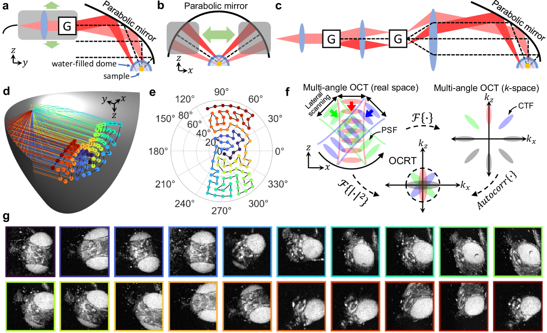
Figure 1: Novel parabolic-mirror-based imaging system enables multi-view imaging over wide angular ranges for OCRT. (a-b) Schematic of our parabolic-mirror-based OCRT imaging system, featuring a 2D translating probe that angularly scans a collimated beam with galvanometers (G). The sample is placed at the center of a water-filled glass optical dome. (c) The same result can be achieved without 2D translation using another set of galvanometers. (d) 3D visualization of the angular coverage by a parabolic mirror via central chief rays for each of the 96 lateral probe positions that we used in our experiments. Rays are color-coded by order of acquisition, from purple to red. (e) The corresponding azimuthal and inclination angles of each central chief ray in (d). (f) k-space theory of OCRT. (g) Example en face projections of a 5D OCRT dataset of a fruit fly, color-coded by incidence angle, consistent with (d) and (e). The lateral FOV of each projection is $\sim$1.7 mm².

2.1 Incoherent 3D $k$-space synthesis with OCRT

Although OCT is a coherent imaging modality characterized by a band-pass coherent transfer function (CTF) [5], OCRT differs from 2D [18, 19] and 3D [20] coherent synthetic aperture techniques in that the multi-angle OCT volumes are combined incoherently, that is, by discarding the phase and only operating on intensity (Fig. 1f). As a result, the band-pass CTF effectively becomes demodulated down to a low-pass [5], which can be understood via the Wiener-Khinchin theorem, by which the magnitude-squaring of the OCT image in real-space corresponds to autocorrelation in $k$-space. As a result, the complex exponentials windowed by the band-pass OCT CTF are rephased to a common origin (i.e., DC), so that OCRT doesn’t have the phase stability requirement that many other coherent synthetic aperture approaches have.

Since these demodulated CTFs, or incoherent transfer functions (ITF), overlap at the $k$-space origin, they can be combined to form an expanded ITF when the OCT resolution is anisotropic (Fig. 1f). This is often the case, as the lateral resolution is typically $>$10 µm, while the axial resolution can essentially be tuned independently via the source properties and can be submicrometer [21]. Thus, the lateral resolution increases monotonically with angular coverage (Fig. S1). In the limit of full angular coverage ($\geq$180^∘), the synthesized ITF is isotropic and given by the original OCT axial resolution (or lateral resolution, whichever is better [22]). Finally, because the observed speckle pattern decorrelates as a function of angular separation, we observe significant speckle reduction because of the incoherent angular compounding.

2.2 Plenoptic imaging with parabolic mirrors

To obtain this resolution enhancement, we require OCT volumes acquired over a very wide angular range, ideally without requiring sample rotation to maximize the generality of OCRT. To this end, we replaced the more typical refractive convex imaging objective with a reflective concave parabolic mirror, which allows independent 4D control of sample-incident the 2D lateral position and 2D angle (azimuthal and inclination) via scanners placed conjugate and anticonjugate to the sample [14] (Fig. 1a-c). Parabolic mirrors are infrequently used for imaging because of their tilt-induced aberrations that restrict FOV, often necessitating sample translation [23, 24]. However, we have exploited the quadratic dependence of FOV on lateral spot size when imaging in an off-axis configuration [13] to obtain millimetric FOVs with a lateral resolution of $\sim$15 µm, consistent with conventional OCT systems. We note that this quadratic scaling with lateral resolution is identical to that of the DOF, meaning that tilt aberrations of parabolic mirrors do not add additional FOV constraints on top of the lateral-resolution-DOF tradeoff we seek to circumvent [13]. Our experimental setup also features a water-filled optical dome placed at the mirror’s focus, where the sample is positioned (Fig. 1a,b), to substantially reduce spherical aberrations that would otherwise occur when a focused beam refracts obliquely across a flat RI discontinuity (e.g., coverslip) interface [13].

To test the feasibility of this novel use of parabolic mirrors and optical domes, we translated an angularly scanning collimated beam across the mirror’s half aperture to vary the sample-incidence angle (Fig. 1a,b), noting that the same effect can be achieved rapidly with another pair of galvanometers (Fig. 1c). With this setup, we were able to obtain plenoptic measurements of the samples, resulting in 5D datasets consisting of approximately $1.3\times 1.3\times 1.65$ mm³ volumes over $\pm 75^{\circ}$ and $\pm 25^{\circ}$ about the $y$- and $x$-axes, respectively (Fig. 1d,e). Example en face OCT images from a 5D dataset of a fruit fly, projected across the $z$ dimension, are shown in Fig. 1g.

2.3 Large-scale, joint OCT volume registration and computational 3D reconstruction

Given this 5D plenoptic dataset, the goal of 3D OCRT is to register and superimpose the multi-angle volumes to realize the incoherent 3D $k$-space synthesis and speckle reduction described earlier. The registration algorithm jointly optimizes two sets of parameters: 1) sample-extrinsic, or those describing the positions and orientations of the sample-incident rays, as governed by the imaging system, and 2) sample-intrinsic, or those describing deformation of ray trajectories due to the spatially varying RI.

In theory, the sample-extrinsic parameters are determined by the parabolic mirror’s sole parameter (i.e, its focal length), the entry positions across the mirror aperture, and the angular scan amplitude (for lateral scanning across the sample), and can thus be modeled through analytical ray tracing. In practice, we account for imperfections or misalignments by allowing a separate set of optimizable parameters for each multi-angle OCT volume, controlling the sample-incident angle, telecentricity, lateral scan range, and field curvature, among others. The sample-extrinsic parameters generate the boundary conditions for ray propagation through the sample’s 3D RI distribution, which is coaligned with the 3D backscatter-based reconstruction. For more details on the registration model, see extended methods in Supplementary Note 1.

Both the sample-intrinsic and sample-extrinsic parameters are optimized via stochastic gradient descent in TensorFlow [17] by minimizing the error between the A-scans of each volume and their forward predictions, as well as regularization terms operating on the 3D RI distribution to promote smoothness and enforce object support. This inverse optimization algorithm of OCRT differs from that of many other inverse problems in that the resolution-enhanced, speckle-reduced reconstruction is not itself a directly optimizable parameter, but rather it is generated through superposition of all OCT volumes, akin to the backprojection algorithm of X-ray computed tomography (CT). However, since requiring joint participation of the entire 5D dataset at every gradient descent iteration, though possible in our original 2D implementation [16], would be computationally infeasible, we propose a stratified batching approach that incrementally accumulates the A-scan contributions to the reconstruction voxels jointly with the registration. Thus, for example, in some cases, the parameters may already be fully optimized and OCT volumes registered before the reconstruction is completely formed. For a more detailed description, see extended methods in Supplementary Note 1.

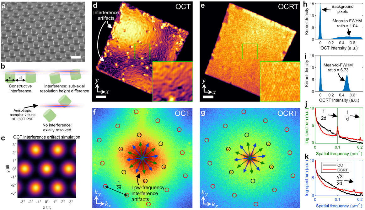
Figure 2: OCRT enhances resolution and reduces interference artifacts (e.g., speckle) of OCT. (a) Scanning electron microscopy of a d = 5-µm, hexagonally-arranged microstamp sample [25]. (b) Sub-resolution differences in pillar heights lead to interference. (c) En face OCT simulation of hexagonal lattice under various tilts predicts interference artifacts. See Fig. S2 for additional simulations. (d) En face OCT image (bilinearly upsampled to match OCRT) does not resolve the pillars and exhibits interference artifacts. (e) 3D OCRT reduces the artifacts and better resolves the pillars. (f) Log power spectral density (PSD) of OCT (black circles: fundamental frequency, $1/2d$; red circles: second harmonics, $1/d$ and $\sqrt{3}/2d$). (g) Log PSD of OCRT. (h) Kernel density estimate (KDE) of (d) exhibits a broad distribution of intensity values due to interference artifacts. (i) KDE of (e), however, exhibits a tight distribution due to speckle reduction. (j) Averaged 1D cross sections of (f) and (g) along green arrows. (k) Averaged 1D cross sections of (f) and (g) along blue arrows. Scale bars, 10 µm in (a), 100 µm in (d), (e).

3 Results

3.1 Validation of lateral resolution enhancement and speckle reduction

We first validated the resolution-enhancing and speckle-reducing capabilities of 3D OCRT by imaging a polydimethylsiloxane (PDMS) microstamp sample, consisting of hexagonally-arranged, 5-µm-diameter, 5-µm-tall cylindrical micropillars with an edge-to-edge spacing of 5 µm (Fig. 2a). Since our OCT system had an axial resolution of 2.1 µm and lateral resolutions of 15.3 ($x$) and 14.6 ($y$) µm (or an anisotropy of $\sim$0.14) from a single view, it does not laterally resolve the 5-µm pillars (Fig. 2d). Furthermore, this OCT image exhibits interference artifacts due to the fact that multiple pillars are probed by the PSF volume (Fig. 2b), consistent with simulated OCT responses to a hexagonal array as a function of tilt (Fig. 2c). Specifically, depending on the local sample tilt or non-telecentricity of the lateral scanning, the resultant axial separation of the pillars can lead to constructive or destructive interference (Fig. 2c), a direct consequence of the axial modulation in the 3D OCT PSF [5]. See also Fig. S2 for OCT predictions matching experimental data, based on fitting-based estimates of microstamp surface normals. This is the same mechanism that underlies speckle formation, which is the interference result of a large number of sub-resolution scatterers.

The 3D OCRT reconstruction much better resolves the pillars and eliminates the interference artifacts of OCT (Fig. 2e). The lateral resolution improvement over OCT can be further appreciated in the power spectra (Fig. 2f,g), in which more of the expected hexagonally-spaced peaks appear in OCRT than OCT, especially the second-harmonic peaks corresponding to the 5-µm features (red circles in Fig. 2f,g). Fig. 2j,k show averaged 1D cross-sections of Fig. 2f,g along the blue and green arrows, with the expected Fourier peaks indicated with vertical lines. From these 1D plots, it is clear that OCRT contains the expected second-harmonic peaks, while OCT does not. The reduction of interference artifacts is also apparent, as Fig. 2f exhibits strong low-frequency artifacts that are absent in Fig. 2g. Interference artifact reduction by OCRT is further quantified in Fig. 2h, i, which show the distribution of intensity values of Fig. 2d,e, where that of OCRT is $\sim$6.5$\times$ narrower than that of OCT.

The resolution enhancement results are consistent with theoretical predictions based on Fig. S1. In particular, we expected synthesized $x$ and $y$ lateral resolutions of $\sim$2.4 µm and $\sim$6.6 µm, corresponding to $\pm 75^{\circ}$ and $\pm 25^{\circ}$, respectively, indicating that our 3D OCRT reconstruction should resolve the 5-µm pillars in the $x$ dimension, but not in the $y$ dimension. Indeed, in Fig. 2g, the red-circled peaks (corresponding to 5-µm features) closer to the $k_{x}$-axis are stronger than those closer to the $k_{y}$-axis.

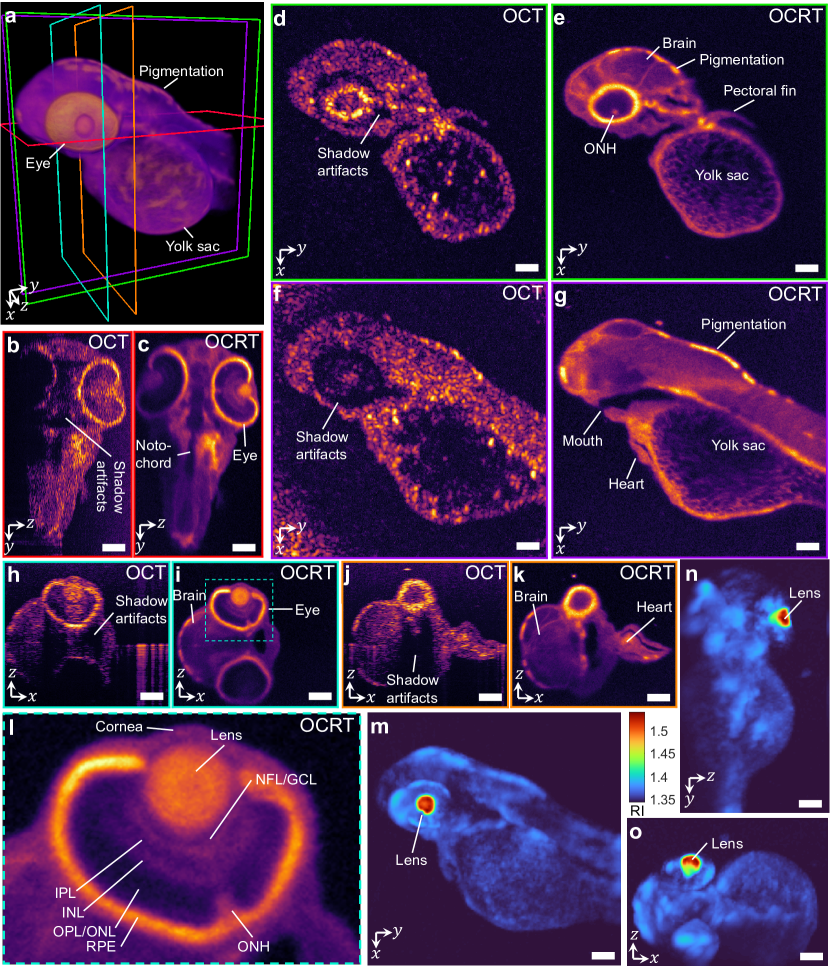
Figure 3: Comparison of conventional OCT and 3D OCRT reconstruction of a 2-dpf zebrafish larva. (a) 3D rendering of OCRT, with color-coded slice locations of cross-sections in subsequent panels. (b-c) Comparison of a $yz$ slice. (d-g) Comparison of $xy$ slices at two different depths. (h-k) Comparison of $xz$ slices at two different $y$ positions. (l) Zoom-in of the eye in (i). NFL: nerve fiber layer, GCL: ganglion cell layer, IPL: inner plexiform layer, INL: inner nuclear layer, OPL: outer plexiform layer, ONL: outer nuclear layer, RPE: retinal pigment epithelium, ONH: optic nerve head. All OCT slices are histogram-matched to the corresponding OCRT slices. (m-o) Maximum intensity projections of the OCRT RI map. Scale bars, 100 µm. See Visualization Computational 3D microscopy with optical coherence refraction tomography for a full 3D comparison.

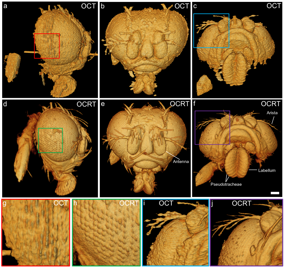
Figure 4: Comparison of conventional OCT (a-c) and 3D OCRT reconstruction (d-f) of a fruit fly head. (a,d) Side view, with zoom-ins (g) and (h), highlighting the clearer reconstruction of the hexagonally-packed lenslets (ommatidia). (b,e) Front view ($z$-axis pointing towards the reader), highlighting clearer bristle reconstructions. (c,f) Bottom view of the 3D renderings, which shows clear reconstruction of the ridges (pseudotracheae) of the labellum and arista (i,j). Scale bar, 100 µm. See Visualization Computational 3D microscopy with optical coherence refraction tomography for a full 3D comparison.

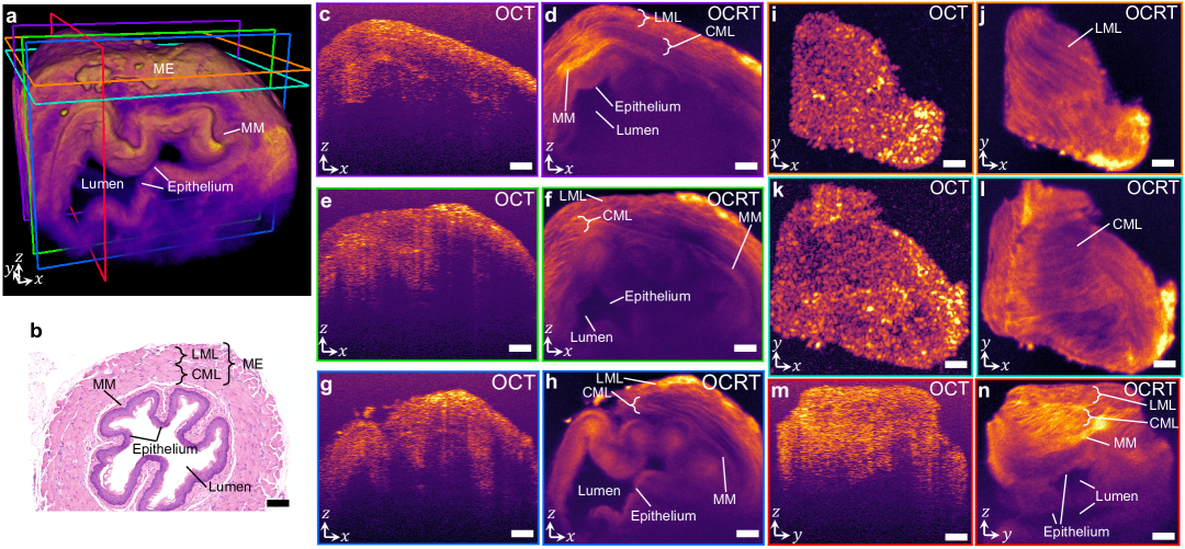
Figure 5: Comparison of OCT and 3D OCRT of mouse esophagus. (a) 3D OCRT rendering, with color-coded slice locations of cross-sections in subsequent panels (MM: muscularis mucosae). (b) H&E-stained histological section. The muscularis externa consists of a longitudinal muscle layer (LML) and a circular muscle layer (CML). (c-h) Comparison of various $xz$ slices. (i-l) Comparison of $xy$ slices st two depths, corresponding to the LML and CML. (m-n) Comparison of $yz$ slices. All OCT slices are histogram-matched to the corresponding OCRT slices. Scale bars, 100 µm. See Visualization Computational 3D microscopy with optical coherence refraction tomography for a full 3D comparison.

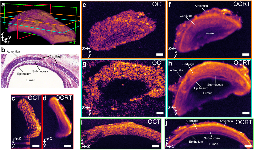
Figure 6: Comparison of OCT and 3D OCRT of mouse trachea. (a) 3D rendering of OCRT, with color-coded slice locations of cross-sections in subsequent panels. (b) H&E-stained histological section. The subsequent panels compare $yz$ slices (c,d), $xy$ slices (e-h), and $xz$ slices (i,j). All OCT slices are histogram-matched to the corresponding OCRT slices. Scale bars, 100 µm. See Visualization Computational 3D microscopy with optical coherence refraction tomography for a full 3D comparison.

3.2 Biological results

To demonstrate the generality of our new 3D OCRT implementation, we imaged and reconstructed several fixed samples: a zebrafish larva at 2 days post fertilization (dpf) (Fig. 3, Visualization Computational 3D microscopy with optical coherence refraction tomography), the head of an adult fruit fly (Fig. 4, Visualization Computational 3D microscopy with optical coherence refraction tomography), and various mouse tissue (Figs. 5, 6; Visualizations Computational 3D microscopy with optical coherence refraction tomography, Computational 3D microscopy with optical coherence refraction tomography). All samples were embedded in 2% agarose (w/v) and immersed in water.

In all cases, the 3D OCRT reconstructions offered substantial improvements over conventional OCT, owing not only to both the lateral resolution enhancement and speckle reduction, but also enhanced penetration depth, despite our imaging system not having access to both sides of the sample (in contrast to our original demonstration [16]). Even in relatively transparent samples like zebrafish larvae, the speckle noise in OCT obscures many features that are revealed in OCRT (Fig. 3, Visualization Computational 3D microscopy with optical coherence refraction tomography). The improvements are especially apparent in the en face slices through the head and yolk sac of the zebrafish larvae, whose original OCT resolution is poor in both dimensions (Fig. 3d-g). Fine reticular structures in the yolk sac unresolvable by OCT are apparent in 3D OCRT. OCT also exhibits strong shadowing from the eye, as most directly apparent in Fig. 3b,h,j. This results in artifacts such as a dark ring around and below the base of the 2-dpf zebrafish larva’s eye (Fig. 3d,f) that is recovered by OCRT (Fig. 3e,g). OCRT also reveals retinal layers and the optic nerve head (Fig. 3e,i,l), which are not apparent in OCT (Fig. 3d,h). Visualization Computational 3D microscopy with optical coherence refraction tomography shows a full flythrough comparison of the 3D OCRT and OCT volumes. Finally, the reconstructed RI maps of OCRT indicate a highly refractive (n $>$ 1.5) lens (Figs. 3m-o), consistent with previous findings [26].

OCRT applied to an adult fruit fly (Fig. 4, Fig. S3, Visualization Computational 3D microscopy with optical coherence refraction tomography) also shows substantial improvement over OCT. Thanks to the speckle reduction and lateral resolution enhancement, the hexagonal packing of the individual micro lenslets (ommatidia) of the compound eye (see Fig. S3 and Supplementary Note 2) and the bristles (hairs) and aristae (branched bristles extending from the antennae) are better resolved by 3D OCRT. OCT, however, exhibits artificially bright and dark signals in the bristles and ommatidia, which are coherent interference artifacts not present in OCRT. OCRT also resolves the pseudotracheae on the labellum (tip of the extension from the mouth) (Fig. 4f).

3D OCRT also offers significant improvements over OCT in mouse tissue, such as esophagus (Fig. 5, Visualization Computational 3D microscopy with optical coherence refraction tomography). Notably, OCRT reveals the muscle fibers of the muscularis externa (ME), which consists of two layers – the outer longitudinal muscle layer (LML) and the inner circular muscle layers (CML), which can be distinguished in the en face depth slices in Figs. 5j and 5l by the change in muscle fiber orientations. These two layers are also visible in the $xz$ cross-sections (Fig. 5d,f,h). This enhanced visualization is attributable to both speckle reduction and resolution enhancement, as obliquely-oriented fibers cannot be resolved by poor OCT lateral resolutions. Below the ME, we can identify the muscularis mucosae (MM), epithelium, and lumen, especially in the cross-sectional cuts of the esophagus shown in Fig. 5d,f,h,n, consistent with hematoxylin and eosin (H&E)-stained histological sections (Fig. 5b). The MM is the thin hyperreflective layer in between the CML and the epithelium. All of these layers are very difficult to identify in the OCT images (Fig. 5c,e,g,i,k,m). The improvement of OCRT over OCT is especially obvious in the flythroughs in Visualization Computational 3D microscopy with optical coherence refraction tomography, in which the difference in muscle fiber orientations of the LML and CML is very clear for OCRT.

3D OCRT also offers substantial improvements over conventional OCT on mouse trachea (Fig. 6), revealing several layers not readily apparent in OCT, most notably the hyaline cartilage rings, featuring lacunae or small cavities. We can also identify the outer adventitial layer (hyperreflective) as well as the submucosal (hyporeflective) and epithelial layers. The large speckle grains in OCT obscure these layers. Visualization Computational 3D microscopy with optical coherence refraction tomography shows a full flythrough comparison between 3D OCRT and OCT.

Finally, while all the 3D OCRT reconstructions presented so far were formed by taking the mean backscattered signal across all multi-angle views, other operations on the 5D OCRT datasets can yield new label-free information about the sample, which we discuss in Supplementary Note 3. For example, computing the variance across the angular dimensions yields a 3D OCRT reconstruction with orientational contrast [27], highlighting structures within the yolk sac of the zebrafish, muscle fibers in the mouse esophagus, and cartilage in the mouse trachea (Fig. S4).

4 Discussion

We have presented 3D OCRT, a new computational volumetric imaging technique that substantially improves the image quality of OCT volumes through lateral resolution enhancement and speckle reduction. Furthermore, we have demonstrated a novel use of parabolic mirrors for multi-view imaging over very wide angular ranges without rotating the sample. Although parabolic mirrors are well known to exhibit “perfect” focusing only when the incident beam is parallel to the mirror’s optic axis due to tilt aberrations, and therefore rarely used as imaging objectives, we demonstrated millimetric FOVs using the weakly-focused, long-DOF beams preferred in OCT. Since the 3D FOV generated by multi-view imaging would be limited by the DOF anyway, the limited lateral FOV of parabolic mirrors, having the same quadratic scaling with lateral resolution as the DOF, do not further restrict the 3D FOV. Thus, OCRT has a resolution advantage compared to optical projection tomography (OPT) for the same 3D FOV, because OCRT decouples resolution from the DOF or FOV.

These improvements over conventional OCT make OCRT competitive with other incoherent (e.g., fluorescence-based) 3D microscopy approaches, such as multiphoton [28] and light-sheet [29, 30] microscopy. OCRT also inherits the many advantages of OCT, such as the longer near-infrared wavelengths typically used, which have higher penetration depths into scattering tissue. Further, while other point-scanning techniques rely on the narrow DOF of high-NA objectives for optical sectioning (e.g., confocal gating), OCT uses coherence gating, which has been shown to more strongly reject out-of-focus and light and therefore have better optical sectioning capabilities [31]. Thus, high-NA objectives are not necessary for high-resolution 3D imaging with OCRT, potentially allowing for longer working distances and less sensitivity to aberrations. Specifically, even though in theory similar rays are used by both high-NA microscopy and OCRT, the former requires all multi-angle rays to be present at the same time to constructively interfere to form a focus. Any rays distorted in amplitude or phase (e.g., by occlusions and aberrations) would thwart the formation of such a focus. However, OCRT uses multi-angle rays sequentially, relying far less on their interference. Thus, OCRT’s imaging depth is less affected by occlusions and aberrations, as evidenced in the zebrafish reconstructions below the highly scattering eye (Fig. 3).

Finally, because we are analyzing OCT and OCRT incoherently using ray-based models, we draw connections to concepts developed in the computer vision community, thus potentially opening new lines of investigations. For example, the 5D OCRT dataset has some similarities to 5D plenoptic function[32] from the field of light field imaging, which the describes the radiance as a function of two angular dimensions across 3D space. One difference is that the plenoptic function is often used to describe imaging of passively illuminated objects, as in photography, whereas OCT actively illuminates the object and observes the 180^∘-backscattered light. As such, the 5D OCRT dataset also bears resemblance to the 6D spatially-varying bidirectional reflectance distribution function (SV-BRDF)[33], which measures radiance as a function of input and output illumination angles (2D each) across an opaque 2D manifold surface. OCRT, however, measures a degenerate version version of the SV-BRDF for the case of equal input and output angles, thus losing two dimensions, while gaining another dimension by measuring this information over 3D instead of 2D space. The two output angle dimensions can be obtained by modifying the OCT system to angle-resolve the back-scattered light, as is done in angle-resolved low-coherence interferometry[34]. Thus, a method based on our parabolic mirror imaging system or other conic-section mirror-based imaging system[13] could lead to faster methods to acquire plenoptic light field or SV-BRDF data for other computational imaging applications.

In summary, 3D OCRT is a new label-free, computational microscopy technique that yields a resolution-enhanced, speckle-reduced reconstruction and a coaligned 3D RI map that reveal new information not apparent in conventional OCT in a wide variety of biological samples. With conceptually straightforward improvements, in particular using faster sources, replacing 2D translation with anti-conjugate galvanometers, and deriving new forms of image contrast from the multi-angle data, 3D OCRT could see wide use in vivo biomedical imaging for basic scientific and diagnostic applications.

Funding This work was funded by the National Science Foundation (CBET-1902904) and the National Institutes of Health (U01EY028079, P30EY005722).

Acknowledgments We thank Z. Kupchinsky and N. Katsanis for providing the fixed zebrafish samples and Ramona Optics for providing the fruit fly sample. We also thank F. Wei for assisting with hardware construction.

Disclosures KCZ, RPM, RQ, AHD, SF, and JAI are inventors on patent applications related to the technologies described in this report.

Data Availability Statement Data underlying the results presented in this paper are available in TBD.

References

- [1] D. Huang, E. A. Swanson, C. P. Lin, J. S. Schuman, W. G. Stinson, W. Chang, M. R. Hee, T. Flotte, K. Gregory, C. A. Puliafito et al., “Optical coherence tomography,” \JournalTitleScience 254, 1178–1181 (1991).
- [2] W. Wieser, W. Draxinger, T. Klein, S. Karpf, T. Pfeiffer, and R. Huber, “High definition live 3d-oct in vivo: design and evaluation of a 4d oct engine with 1 gvoxel/s,” \JournalTitleBiomedical optics express 5, 2963–2977 (2014).
- [3] O. M. Carrasco-Zevallos, C. Viehland, B. Keller, M. Draelos, A. N. Kuo, C. A. Toth, and J. A. Izatt, “Review of intraoperative optical coherence tomography: technology and applications,” \JournalTitleBiomedical optics express 8, 1607–1637 (2017).
- [4] B. Karamata, K. Hassler, M. Laubscher, and T. Lasser, “Speckle statistics in optical coherence tomography,” \JournalTitleJOSA A 22, 593–596 (2005).
- [5] K. C. Zhou, R. Qian, A.-H. Dhalla, S. Farsiu, and J. A. Izatt, “Unified k-space theory of optical coherence tomography,” \JournalTitleAdvances in Optics and Photonics 13, 462–514 (2021).
- [6] Z. Ding, H. Ren, Y. Zhao, J. S. Nelson, and Z. Chen, “High-resolution optical coherence tomography over a large depth range with an axicon lens,” \JournalTitleOptics Letters 27, 243–245 (2002).
- [7] R. Leitgeb, M. Villiger, A. Bachmann, L. Steinmann, and T. Lasser, “Extended focus depth for fourier domain optical coherence microscopy,” \JournalTitleOptics Letters 31, 2450–2452 (2006).
- [8] K.-S. Lee and J. P. Rolland, “Bessel beam spectral-domain high-resolution optical coherence tomography with micro-optic axicon providing extended focusing range,” \JournalTitleOptics Letters 33, 1696–1698 (2008).
- [9] L. Liu, J. A. Gardecki, S. K. Nadkarni, J. D. Toussaint, Y. Yagi, B. E. Bouma, and G. J. Tearney, “Imaging the subcellular structure of human coronary atherosclerosis using micro–optical coherence tomography,” \JournalTitleNature Medicine 17, 1010–1014 (2011).
- [10] T. S. Ralston, D. L. Marks, P. S. Carney, and S. A. Boppart, “Interferometric synthetic aperture microscopy,” \JournalTitleNature Physics 3, 129–134 (2007).
- [11] A. Desjardins, B. Vakoc, G. Tearney, and B. Bouma, “Speckle reduction in oct using massively-parallel detection and frequency-domain ranging,” \JournalTitleOptics Express 14, 4736–4745 (2006).
- [12] O. Liba, M. D. Lew, E. D. SoRelle, R. Dutta, D. Sen, D. M. Moshfeghi, S. Chu, and A. de La Zerda, “Speckle-modulating optical coherence tomography in living mice and humans,” \JournalTitleNature Communications 8, 1–13 (2017).
- [13] K. C. Zhou, A.-H. Dhalla, R. P. McNabb, R. Qian, S. Farsiu, and J. A. Izatt, “High-speed multi-view imaging approaching 4pi steradians using conic section mirrors: theoretical and practical considerations,” \JournalTitleJOSA A 38 (2021).
- [14] O. Carrasco-Zevallos, D. Nankivil, B. Keller, C. Viehland, B. J. Lujan, and J. A. Izatt, “Pupil tracking optical coherence tomography for precise control of pupil entry position,” \JournalTitleBiomedical Optics Express 6, 3405–3419 (2015).
- [15] J. Yao, P. Meemon, M. Ponting, and J. P. Rolland, “Angular scan optical coherence tomography imaging and metrology of spherical gradient refractive index preforms,” \JournalTitleOptics Express 23, 6428–6443 (2015).
- [16] K. C. Zhou, R. Qian, S. Degan, S. Farsiu, and J. A. Izatt, “Optical coherence refraction tomography,” \JournalTitleNature Photonics 13, 794–802 (2019).
- [17] M. Abadi, A. Agarwal, P. Barham, E. Brevdo, Z. Chen, C. Citro, G. S. Corrado, A. Davis, J. Dean, M. Devin, S. Ghemawat, I. Goodfellow, A. Harp, G. Irving, M. Isard, Y. Jia, R. Jozefowicz, L. Kaiser, M. Kudlur, J. Levenberg, D. Mané, R. Monga, S. Moore, D. Murray, C. Olah, M. Schuster, J. Shlens, B. Steiner, I. Sutskever, K. Talwar, P. Tucker, V. Vanhoucke, V. Vasudevan, F. Viégas, O. Vinyals, P. Warden, M. Wattenberg, M. Wicke, Y. Yu, and X. Zheng, “TensorFlow: Large-scale machine learning on heterogeneous systems,” (2015).
- [18] S. A. Alexandrov, T. R. Hillman, T. Gutzler, and D. D. Sampson, “Synthetic aperture fourier holographic optical microscopy,” \JournalTitlePhysical Review Letters 97, 168102 (2006).
- [19] G. Zheng, R. Horstmeyer, and C. Yang, “Wide-field, high-resolution fourier ptychographic microscopy,” \JournalTitleNature Photonics 7, 739–745 (2013).
- [20] V. Lauer, “New approach to optical diffraction tomography yielding a vector equation of diffraction tomography and a novel tomographic microscope,” \JournalTitleJournal of Microscopy 205, 165–176 (2002).
- [21] B. Povazay, K. Bizheva, A. Unterhuber, B. Hermann, H. Sattmann, A. F. Fercher, W. Drexler, A. Apolonski, W. Wadsworth, J. Knight et al., “Submicrometer axial resolution optical coherence tomography,” \JournalTitleOptics Letters 27, 1800–1802 (2002).
- [22] K. C. Zhou, R. Qian, S. Farsiu, and J. A. Izatt, “Spectroscopic optical coherence refraction tomography,” \JournalTitleOptics Letters 45, 2091–2094 (2020).
- [23] M. A. Lieb and A. J. Meixner, “A high numerical aperture parabolic mirror as imaging device for confocal microscopy,” \JournalTitleOptics Express 8, 458–474 (2001).
- [24] T. Ruckstuhl and S. Seeger, “Attoliter detection volumes by confocal total-internal-reflection fluorescence microscopy,” \JournalTitleOptics Letters 29, 569–571 (2004).
- [25] “Research micro stamps,” https://researchmicrostamps.com/.
- [26] T. M. Greiling and J. I. Clark, “The transparent lens and cornea in the mouse and zebra fish eye,” in Seminars in cell & developmental biology, vol. 19 (Elsevier, 2008), pp. 94–99.
- [27] B. J. Lujan, A. Roorda, R. W. Knighton, and J. Carroll, “Revealing Henle’s fiber layer using spectral domain optical coherence tomography,” \JournalTitleInvestigative Ophthalmology & Visual Science 52, 1486–1492 (2011).
- [28] W. R. Zipfel, R. M. Williams, and W. W. Webb, “Nonlinear magic: multiphoton microscopy in the biosciences,” \JournalTitleNature Biotechnology 21, 1369–1377 (2003).
- [29] M. B. Ahrens, M. B. Orger, D. N. Robson, J. M. Li, and P. J. Keller, “Whole-brain functional imaging at cellular resolution using light-sheet microscopy,” \JournalTitleNature Methods 10, 413–420 (2013).
- [30] B.-C. Chen, W. R. Legant, K. Wang, L. Shao, D. E. Milkie, M. W. Davidson, C. Janetopoulos, X. S. Wu, J. A. Hammer, Z. Liu et al., “Lattice light-sheet microscopy: imaging molecules to embryos at high spatiotemporal resolution,” \JournalTitleScience 346 (2014).
- [31] J. A. Izatt, M. R. Hee, G. M. Owen, E. A. Swanson, and J. G. Fujimoto, “Optical coherence microscopy in scattering media,” \JournalTitleOptics Letters 19, 590–592 (1994).
- [32] E. H. Adelson, J. R. Bergen et al., The plenoptic function and the elements of early vision, vol. 2 (Vision and Modeling Group, Media Laboratory, Massachusetts Institute of …, 1991).
- [33] F. E. Nicodemus, “Directional reflectance and emissivity of an opaque surface,” \JournalTitleApplied optics 4, 767–775 (1965).
- [34] A. Wax, C. Yang, V. Backman, K. Badizadegan, C. W. Boone, R. R. Dasari, and M. S. Feld, “Cellular organization and substructure measured using angle-resolved low-coherence interferometry,” \JournalTitleBiophysical Journal 82, 2256–2264 (2002).