Near Perfect GAN Inversion

Abstract

To edit a real photo using Generative Adversarial Networks (GANs), we need a GAN inversion algorithm to identify the latent vector that perfectly reproduces it. Unfortunately, whereas existing inversion algorithms can synthesize images similar to real photos, they cannot generate the identical clones needed in most applications. Here, we derive an algorithm that achieves near perfect reconstructions of photos. Rather than relying on encoder- or optimization-based methods to find an inverse mapping on a fixed generator $G(\cdot)$, we derive an approach to locally adjust $G(\cdot)$ to more optimally represent the photos we wish to synthesize. This is done by locally tweaking the learned mapping $G(\cdot)$ s.t. $\|{\bf x}-G({\bf z})\|<\epsilon$, with ${\bf x}$ the photo we wish to reproduce, ${\bf z}$ the latent vector, $\|\cdot\|$ an appropriate metric, and $\epsilon>0$ a small scalar. We show that this approach can not only produce synthetic images that are indistinguishable from the real photos we wish to replicate, but that these images are readily editable. We demonstrate the effectiveness of the derived algorithm on a variety of datasets including human faces, animals, and cars, and discuss its importance for diversity and inclusion.

Figure 1: (a) Two real photos. The goal of GAN inversion is to find a latent code that synthesizes an image that is as similar as possible to that in (a). Synthesizing these photos is hard as made evident by the results obtained using state-of-the-art GAN inversion algorithms as shown in (b) and (c). In (d) we show the results of the method proposed in this paper. As we can see, the synthesized images are almost identical clones with only tiny differences not visible to the naked eye. Furthermore, these clones are readily editable using standard GAN editing algorithms as shown in (e-f). Results best seen at a 600% zoom.

1 Introduction

Generative Adversarial Networks (GANs) have seen dramatic improvement on image photo-realism in recent years [14, 21, 18, 9, 19]. Crucially, GAN-generated images are editable, enabling a number of previously difficult to envision applications. For example, in movies, ads, virtual reality, video games and e-commerce, we can now edit existing photos to improve or showcase image variants that are difficult, costly, or impossible to film. For instance, a face can be shown to be younger or have a different hair color or style.

To edit real photos though, we need a GAN inversion algorithm, Fig. 1. More formally, the generator function $G({\bf z})={\bf x}$ maps a latent vector ${\bf z}\in\mathcal{Z}\subseteq\mathbb{R}^{q}$ into an image ${\bf x}\in\mathcal{X}\subseteq\mathbb{R}^{p}$, with $q\ll p$. GAN inversion is the problem of finding ${\bf z}$ given ${\bf x}$, i.e., ${\bf z}=G^{-1}({\bf x})$. However, unlike Normalizing Flows and auto-encoders, inverting $G(\cdot)$ in GANs is generally impossible. To solve this problem, researchers use encoder or optimization approaches to solve

$$\min\|G(h(\mathbf{x}))-\mathbf{x}\|$$ (1)

with the algorithm converging to a solution iff $\|G(h(\mathbf{x}))-\mathbf{x}\|<\epsilon$, and where $\|\cdot\|$ is a metric in image space $\mathcal{X}$, $h:\mathcal{X}\mapsto\mathcal{Z}$, and $\epsilon>0$ is small.

Optimization algorithms find the latent vector representation of a given image by optimizing $h(\cdot)$ as in Eq. 1 from a starting guess [24, 13, 1, 2]. In encoder approaches $h(\cdot)$ is usually a deep network trained to map from $\mathcal{X}$ onto $\mathcal{Z}$ and optimize Eq. 1 over a training set [26, 26, 28, 4, 10]. There are also hybrid approaches [11, 6].

Hence, crucially, optimization and encoder approaches assume that the mapping $G(\cdot)$ is able to synthesize the desirable photo ${\bf x}$. However, given the large variety of all possible photos $\mathcal{X}$, this assumption will typically not hold, resulting in sub-par reconstruction results, Fig. 1(b, c).

While optimization- and encoder-based approaches optimize or learn $h(\cdot)$ while fixing $G(\cdot)$, our key contribution is to show we can fix $h(\cdot)$ and locally tune $G(\cdot)$ instead.

Fig. 1(d) shows the reconstruction results of our approach compared to state-of-the-art methods Fig. 1(b,c). GAN editing can then be applied to the reconstructed images, yielding photo-realistic image variants, Fig. 1(e-g).

The derived solution is not only scientifically novel, it is also essential for many real-world applications. Semantic manipulation of real photos is only meaningful if the edited images are seen as realistic variants of the original photos, e.g., the exact same face and background but with a different eye gaze, mouth shape or facial hair as illustrated in Fig. 1(e-g). Additionally, as out-of-sample photos are more likely to be ill-inverted, most current algorithms cannot be used on photos of groups under-represented in the training data, which may include ethnic, racial, gender, age, religious, cultural, job/occupation, etc. Our solution solves these important limitations.

We provide extensive comparative evaluations on several datasets against the state of the art, showing that our reconstructed images keep their photo-realism even after being edited, and demonstrate that our derived algorithm is equally applicable to under-represented groups, increasing diversity and inclusion.

2 Related Work

Two GAN inversion algorithms have been proposed in the literature: “projection via optimization” and “projection via a feedforward network”, i.e., optimization- and an encoder-based method [39].

2.1 Optimization-based inversion

Optimization-based methods require making three choices. First, a loss to measure the similarity between the real photo and the reconstructed image; second, a latent space over which the loss function may be optimized; and, third, the optimization criterion. Early works like [24] explore the usage of the likelihood loss in a Gaussian latent space. Others [13] perform stochastic clipping, limiting the magnitude of the gradient as it optimizes image similarity.

2.2 Encoder-based inversion

For encoder-based or learning-based methods as in [36], we require first, an encoder network; second, a loss to measure the similarity between the real photo and the reconstructed image, and third, the output vectors on the latent space. [26] proposed an auto-encoder architecture incorporating a StyleGAN generator, with an explicit mapping learnt from synthetic image. Others use different mapping or latent space representations [28].

Compared to optimization-based methods, encoder-based algorithms enjoy the benefit of faster inference time. To further improve their results, ReStyle [4] defines an iterative residual-based encoder. [10] proposed a latent space encoder with masked input to study the compositionality in GANs latent space. There are also hybrid methods [11, 6], combining the advantages of encoder- and optimization-based method.

2.3 Limitations of these methods

The pre-trained generator is fixed in both the optimization- and encoder-based methods. Since there is no guarantee that the photos we wish to replicate synthetically can be generated by $G(\cdot)$, these methods typically yield disappointing results (Fig. 1). Moreover, groups that are under-represented in the training set cannot be reproduced accurately, lowering diversity and decreasing inclusion.

In our work we propose a third way: we allow the generator to be updated locally about the query latent vector. We optimize this update to obtain a faithful reproduction of the photo of interest. This yields better reconstruction accuracy while maintaining editability of the image.

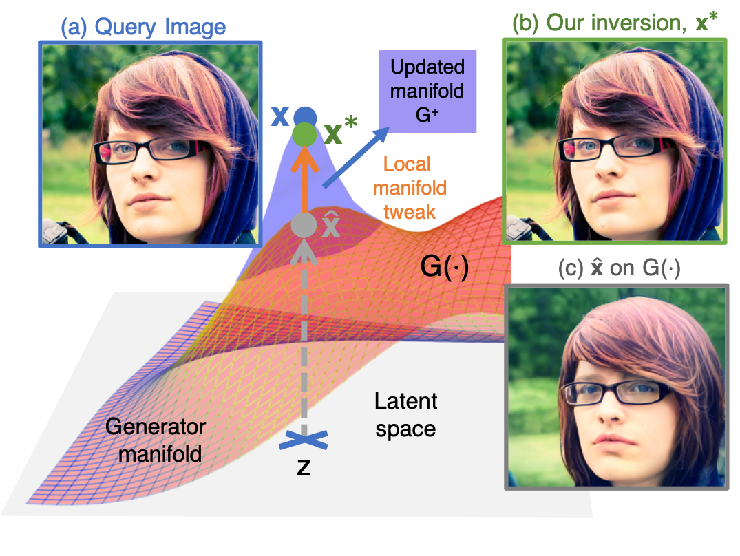
Figure 2: The query photo we wish to synthesize is given by ${\bf x}$. Given a pre-trained GAN model, its generator function $G(\cdot)$ can, at best, synthesize image $\hat{\bf x}$. That is, $\hat{\bf x}$ is the point on the manifold that is closest to ${\bf x}$. This paper proposes an algorithm to locally tweak $G(\cdot)$ to include an image ${\bf x}^{*}$ s.t. $\|{\bf x}-{\bf x}^{*}\|<\epsilon$. We refer to the new tweaked manifold as $G^{+}(\cdot)$. The original $G(\cdot)$ is show in orange and the tweaked $G^{+}(\cdot)$ in blue. The latent space is represented as a gray plane at the bottom.

3 Method

3.1 Problem definition

For a given query photo $\mathbf{x}\in\mathcal{X}$, we want to obtain its corresponding latent code $\mathbf{z}\in\mathcal{Z}$ that reconstructs $\mathbf{x}$ as accurately as possible, i.e., $G({\bf z})={\bf x}^{*}$, with $\|{\bf x}^{*}-{\bf x}\|<\epsilon$.

Previous encoder- and optimization-based methods focus on optimizing $h(\cdot)$ while keeping $G(\cdot)$ frozen. To reconstruct $\mathbf{x}$, these previous methods have to operate under the assumption that ${\bf x}^{*}$ is on the manifold defined by $G(\cdot)$, i.e., $\exists\,{\bf z}\in\mathcal{Z}\text{ s.t. }G({\bf z})={\bf x}^{*}$.

When $\mathbf{x}$ does not lie on or very close to the pre-trained manifold defined by $G(\cdot)$, the best these methods can do is to retrieve its nearest projection $\mathbf{\hat{x}}$ as illustrated in Fig. 2. This figure shows an example where the query photo ${\bf x}$ is not on the manifold defined by $G(\cdot)$, which is shown as an orange manifold. Thus, GAN inversion methods can at best synthesize the image $\hat{\bf x}$. $\hat{\bf x}$ is the image on the manifold defined by $G(\cdot)$ that is closest to ${\bf x}$; here closeness is given by an orthographic projection onto the manifold. Our proposal is an algorithm that locally tweaks this manifold $G(\cdot)$ to include the image ${\bf x}^{*}$, an image that is as close as possible to the query photo ${\bf x}$. This is shown as a blue extension of the manifold in the figure.

3.2 Tweaking the manifold locally

Let us now derive the method to update the manifold defined by the generator locally.

Note we cannot simply modify the manifold $G(\cdot)$ in any random way that happens to include ${\bf x}$. This is because in addition to including our query image ${\bf x}$, the manifold should only change locally and in a way that allows us to edit the synthesized version of ${\bf x}$ as easily as we edit any other synthetic image. In addition, we need to ensure that these edits yield synthetic image variants that look as realistic as the original photo.

To successfully edit the manifold locally, we first need to find $\hat{\bf x}$, i.e., the closest point to ${\bf x}$ we can find on the manifold. To this end, we can use any of the existing approaches described above. That is, we optimize $h(\cdot)$ by keeping $G(\cdot)$ fix.

Once we have $\hat{\bf x}$, we fix $h(\cdot)$ and let $G(\cdot)$ change locally about $\hat{\bf x}$ to include ${\bf x}^{*}$, Fig. 2. Our goal is to make the smallest change possible while maintaining the desirable properties of the pre-trained $G(\cdot)$, e.g., we can edit images in a number of controllable ways.

We do this by combining two loss functions. The first loss function $\mathcal{L}_{\text{local}}$ is tasked to locally tweak the manifold to include ${\bf x}$ by making the distance from ${\bf x}$ to ${\bf x}^{*}$ as small as possible and keeping the properties of the manifold intact. The second loss function $\mathcal{L}_{\text{global}}$ ensures the rest of the manifold does not change.

3.3 Local loss

For the manifold defined by $G(\cdot)$ to generate ${\bf x}$, there needs to be a latent vector ${\bf z}$ s.t. $G({\bf z})$ is as similar to ${\bf x}$ as possible. We can compute this using a reconstruction loss function $\mathcal{L}_{\text{recon}}({\bf x}_{1},{\bf x}_{2})$ that measure the similarity between ${\bf x}_{1}$ and ${\bf x}_{2}$, with ${\bf x}_{i}\in\mathcal{X}$.

Because our goal is to synthesize an image that is as visually similar to the query photo as possible, we choose to use the Laplacian pyramid [3, 8] loss function as $\mathcal{L}_{\text{recon}}(\cdot,\cdot)$. Note, however, that other similarity losses could be used.

Let $\mathcal{L}_{\text{recon}}=\text{LaplacianPyramid}(\mathbf{x},G({\bf z}))$ be the reconstruction loss computed using the Laplacian pyramid, calculated by summing over mean L1 differences across all levels of a Laplacian pyramid of ${\bf x}$ and $G({\bf z})$. We can now find ${\bf z}$ s.t. $G({{\bf z}})=\hat{\bf x}$ and then optimize $\mathcal{L}_{\text{recon}}$ until $\mathcal{L}_{\text{recon}}<\epsilon$.

To encourage that the tweaked manifold is editable and maintains all other desirable properties, we regularize this solution with an adversarial loss, $\mathcal{L}_{\text{adv\_local}}$. Specifically, we consider, $\mathcal{L}_{\text{adv\_local}}=\log D(\mathbf{x})+\log(1-D(G({\bf z})))$, where $D(\cdot)$ is the discriminator.

The combined local loss is thus given by,

$$\mathcal{L}_{\text{local}}=\mathcal{L}_{\text{recon}}+\lambda\mathcal{L}_{\text{adv\_local}},$$ (2)

where $\lambda$ is the regularizing term. Here too we find ${\bf z}$ s.t. $G({{\bf z}})=\hat{\bf x}$ and then optimize $\mathcal{L}_{\text{local}}$.

3.4 Global cohesion

We still need to ensure that the rest of the manifold does not change. This is to make sure that the model keeps any previous training and tweaking we have applied. We do this by computing a global loss function to enforce overall stability of the manifold.

To this end we use the loss of the pre-trained GAN model. For example, when using StyleGAN2, our global loss will be

$$\mathcal{L}_{\text{global}}=\mathbb{E}_{\mathbf{x}\sim p_{\mathbf{x}}}[\log D(\mathbf{x})]+\mathbb{E}_{\mathbf{z}\sim p_{\mathbf{z}}}[\log(1-D(G(\mathbf{z})))].$$ (3)

where $\mathbf{x}$, $\mathbf{z}$, $p_{\mathbf{x}}$ and $p_{\bf z}$ are defined exactly as in the pre-trained GAN. If the generator architecture changes, it will be necessary to use the $\mathcal{L}_{\text{global}}$ associated to that GAN model.

Putting everything together, the final loss function to optimize is given as

$$\mathcal{L}=\mathds{1}_{p}[\mathcal{L}_{\text{local}}]+\mathcal{L}_{\text{global}}$$ (4)

where $\mathds{1}_{p}$ is an indicator function activated with probability $p$, with $p$ generally kept small to attain good convergence and stability on $G(\cdot)$. The lower the $p$, the less frequent $\mathcal{L}_{\text{local}}$ term updates during training. For example, when $p=1/8$, $\mathcal{L}_{\text{local}}$ will be updated once for every eight updates on $\mathcal{L}_{\text{global}}$.

The proposed GAN inversion method is summarized in Algorithm 1. We call this algorithm Clone since the synthesized image is a near clone of the real photo.

Once this process is completed, the updated generator $G^{+}$ is used to edit the image $\mathbf{x}^{*}$. Editing techniques that do not require training (e.g., StyleSpace [35]) can be directly applied on $G^{+}$. Methods that require model training (e.g., WarpedGANSpace [33], Image2StyleGAN [2]) can also be directly applied without re-training on $G^{+}$, since $G^{+}$ preserve most manifold structure as the pre-trained generator.

Algorithm 1 Pseudo-code of Clone, the proposed GAN inversion algorithm.

Input: Query image $\mathbf{x}$, pre-trained model $G(\cdot)$ and $D(\cdot)$, the training set $\mathcal{X}_{train}$, hyper-parameters $\{p,\lambda,\epsilon\}$, an inversion function $h(\cdot)$, maximum number of iterations $T$.
      Output: Synthesized image $\mathbf{x}^{*}$, generator $G^{+}(\cdot)$.

1:Let $\mathbf{z}\leftarrow h(\mathbf{x})$.

2:Let $G^{(0)}\leftarrow G$.

3:Let $D^{(0)}\leftarrow D$.

4:for $t=1$ to $T$ do

5:     $u\sim\text{Uniform}[0,1)$

6:     if $u<p$ then

7:         Calculate $\mathcal{L}_{\text{local}}$ as in Eq. 2

8:     else

9:         $\mathcal{L}_{\text{local}}=0$      

10:     Compute $\mathcal{L}_{\text{global}}$ as in Eq. 3.

11:     $\mathcal{L}=\mathcal{L}_{\text{local}}+\mathcal{L}_{\text{global}}$.

12:     $G^{(t+1)}$ is updated with $\partial\mathcal{L}/\partial G^{(t)}$.

13:     $D^{(t+1)}$ is updated with $\partial\mathcal{L}/\partial D^{(t)}$.

14:     if $\mathcal{L}_{\text{recon}}<\epsilon$ then

15:         Stop      

16:$G^{+}(\cdot)\leftarrow G^{(t+1)}(\cdot)$.

17:$\mathbf{x}^{*}\leftarrow G^{+}({\bf z})$.

4 Experiments

In this section, we provide quantitative as well as qualitative comparisons of the proposed GAN inversion algorithms against state-of-the-art techniques.

4.1 Implementation details

We demonstrate the performance of the proposed GAN inversion algorithm on six datasets, Flickr-Faces-HQ Dataset (FFHQ) [20, 22], CelebA-HQ [17], Stanford Cars [23], LSUN-Cars [37], Animal Faces HQ in-the-Wild (AFHQ-Wild) [12], and LSUN-Horses [37]. The resolution of these images go from from $1,024\times 1,024$ to $256\times 256$ pixels.

The generator in StyleGAN2 uses a neural network architecture that receives a style latent code at each of its layers. To achieve a disentangled latent space, the StyleGAN2 architecture employs two decoupled network components referred to as the mapping network and the synthesis network.

A Normal distribution in $\mathcal{Z}$-space is transformed to $\mathcal{W}$-space via the mapping network, which is further extended to create $\mathcal{W+}$ [2]. In the experiments shown below, we recover the latent codes in $\mathcal{W+}$ space. And, in our experiments, we start with pre-trained StyleGAN2 models and apply the proposed GAN inversion algorithms detailed in Section 3.

In our experiments, we use $p=1/4,1/8,1/32,1/16$ for the Faces (FFHQ, CelebA-HQ), Cars (LSUN-Cars, Stanford-Cars), AFHQ and LSUN-Horses experiments, respectively. We use $\lambda=10$ in Eq. 2 for Faces, Cars and AFHQ experiments and $\lambda=20$ for LSUN-Horses experiment. These parameters are selected by a simple heuristic which is described in Supplemental File. When experimenting with additional values for these parameters, we obtained very similar results to those reported below. In all experiments, we set $\epsilon<.001$ and $T=100K$. Additional details are given in the Supplementary File.

The starting point for ${\bf x}^{*}$ is given by the Restyle encoder algorithm [4]. We have also tested the use of optimization-based algorithms to initialize ${\bf x}^{*}$. This yielded identical results.

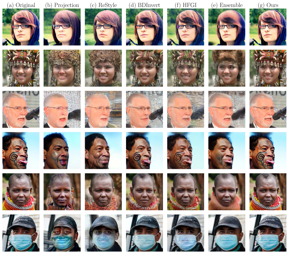
Figure 3: Comparative results of our method against five state-of-the-art GAN inversion algorithms. (a) Query photo we wish to synthesize. (b) A state-of-the-art optimization-based GAN inversion method [22]. (c-e) State-of-the-art encoder methods [4, 16, 34]. (f) A state-of-the-art hybrid method [11]. (g) Results obtained with the approach proposed in this paper. Note how the proposed method is able to synthesize a clone that is indistinguishable from the original photo. First three rows are clones of samples found in the set used to train $G(\cdot)$. Last three rows show results on out-of-sample photos. The proposed algorithm is able to synthesize perfect clones in both, out-of-sample and in-sample, cases. All images and photos are of 1M pixels. Synthesized results best seen at 600% zoom.

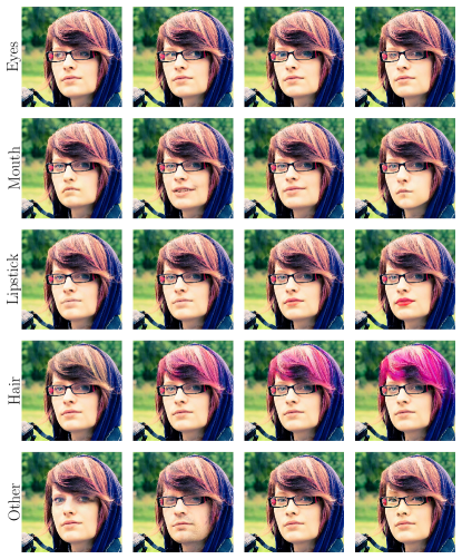
Figure 4: The synthetic clones recovered by the proposed algorithm are readily editable using standard, off-the-shelf algorithms. While other GAN inversion methods require training their own traversal functions, our proposed solution allows for the use of standard, pre-computed traversals. Here, we show eight edits using StyleSpace [35] on the clone of the photo shown in Figure 3(a). Note the high photo-realism of these images.

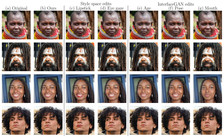
Figure 5: State-of-the-art GAN inversion algorithms cannot accurately synthesize photos of people and cultures that are under-represented in the dataset used to pre-train the GAN. This is because $G(\cdot)$ is fixed and has not been trained to represent those groups and cultures. This leads to issues of diversity and inclusion. The algorithm described in this paper addresses these limitations by allowing local tweaks to $G(\cdot)$. In (a-b), we show results of our GAN inversion algorithm on photos of people with hair styles as well as facial scarification, tattoos, and cultural marks not well represented or not represented at all in the set used to pre-train the GAN. In (c-d), we show edits of the images synthesized by our approach using the algorithm of [35]. (e-g) shows edits using the algorithm of [29].

4.2 Qualitative results on human faces

We first show our algorithm is able to solve the inversion problem of the target photos with extreme accuracy, even for out-of-sample photos, Fig. 3. The figure provides comparative results against Restyle [4], BDInvert [16], High-Fidelity GAN Inversion (HFGI) [34], and Ensemble (a hybrid optimization+encoder approach) [11].

As seen in Fig. 3, the proposed algorithm is able to synthesize image clones that are basically identical to the real photos. The synthesized images include difficult-to-reconstruct, high-frequency details such as hair and skin texture. (Figure results best seen at a 600% zoom.)

Second, to demonstrate that such accurate reconstructions come at no adverse effect on the ability to edit the synthetic clone, we show a number of image modifications using standard algorithms [35, 29], Fig. 4.

Specifically, we chose two state-of-the-art GAN editing techniques. The first is StyleSpace [35], which discovers dimensions in latent space that control specific image attributes such as eye gaze, hair color, skin tone, and mouth shape. The second is InterfaceGAN [29], which finds linear traversals that modify a specific semantic attribute.

4.3 Diversity and inclusion

The biases of computer vision and machine learning models are well known and widely reported [27, 32, 7]. These are especially problematic when dealing with human faces due to our attachment of self-worth, identity and cultural values [25]. GANs are not immune from this problem, with pre-trained models carrying the biases of the photos used to define their training sets [15, 5].

The GAN inversion algorithm derived in this paper solves this important problem. Our algorithm is especially good at synthesizing out-of-sample data points. This means, the proposed algorithm successfully synthesizes photos of people and cultures under-represented in the training set. In fact, the proposed inversion algorithm is still able to synthesize a near identical images to their query photos.

Fig. 5 shows several example image clones corresponding to out-of-sample photos. Note how the proposed algorithm is able to synthesize hairstyle, facial tattoos, and cultural jewelry/amulets not included in the training set of the pre-trained GAN model we used.

Importantly, and as shown in the figure, these clones are equally editable to those of in-sample groups and cultures.

4.4 Qualitative results on cars and animals

Fig. 6 shows qualitative results for cars on the Stanford Cars [23] dataset using StyleGAN2 models pre-trained on LSUN-Cars dataset [37]. In (a) we show the query photo we wish to synthesized. Results obtained with state-of-the-art methods are in (b-d). The synthesis results given by our algorithm are in (e). And, in (f), we show a couple edits applied to our synthesized images. As with faces, we see that the proposed approach yields results that are indistinguishable from the original photo.

Fig. 7 shows GAN inversion results of animals on the AFHQ-Wild and LSUN horses datasets. As with faces and cars, all StyleGAN2 models were pre-trained on the same training set and the results shown in the figure computed on an independent set of photos. These two datasets only have pre-train models for two of the GAN inversion models, Projection [22] and ReStyle [4]. Thus, Fig. 7(a) shows the original photo, Fig. 7 (b-c) these state-of-the-art results, and Fig. 7(d) the reconstructions given by the Clone algorithm derived in this paper. In (e), we show three example edits using StyleSpace [35] and the unsupervised approach of [30].

4.5 Quantitative results

Previous sections provided a number of qualitative comparative results on faces, cars and animals.

Table 1 shows the corresponding quantitative results. The first results in this table are computed on the CelebA-HQ [17] face dataset using StyleGAN2 models pre-trained on FFHQ [20]. The second results are on the testing set of the AFHQ-Wild [12] animal dataset using StyleGAN2 models pre-trained on the training set of the same database. The third results are on the testing set of the Stanford Cars [23] dataset using StyleGAN2 models pre-trained on the the training set of the same database.

We used two metrics to report our quantitative results in Table 1. The first is the Mean Squared Error (MSE). This is simply the norm-2 distance between the query photo and the image synthesized by each of the five state-of-the-art methods plus the algorithm presented in this paper. Results are the average over all testing images. Obviously, the lower the MSE, the better, with zero indicating the original photos and the synthesized clones are 100% identical. The second metric is the Learned Perceptual Image Patch Similarity (LPIPS) [38]. LPIPS computes the perceptual similarity of the synthesized image to the query photo. The perceptual similarity is calculated using a visual neural network model. As it is most commonly done, we use VGG [31]. As with MSE, the lower the value of LPIPS, the more visually similar the synthesized images are to the query photos.

As we see in the table, our proposed algorithm achieves MSE values that are at least an order of magnitude lower than those obtained by state-of-the-art methods. This is true regardless of the database and type of object we wish to synthesize. LPIPS confirms the visual similarity of our synthesized images to their corresponding query photos. Not all GAN inversion algorithms have a model available for comparison. When that’s the case, we indicate this with ‘–’ entries in the table.

We refer the reader to the Supplementary Files for additional quantitative and qualitative results.

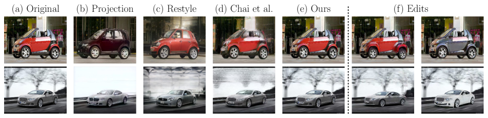
Figure 6: Inversion results on Stanford Cars [23]. (a) Original photo. (b-d) State-of-the-art results. (e) Our results. (f) A couple edits on our reconstruction using [35] and [30].

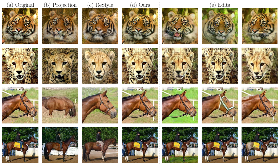
Figure 7: Reconstruction results of the real photos shown in column (a). Projection (an optimization method) [22] results are in column (b), ReStyle (an Encoder-based method) [4] results in column (c), and the results of the approach described in this paper in column (d). In (e), we show three image edits using StyleSpace [35] and the unsupervised algorithm of [30]. The first two rows show results on the AFHQ-Wild database [12]. The last two rows show results on the LSUN Horse dataset [37].

Dataset	CelebA-HQ		Stanford Cars		AFHQ-Wild		LSUN-Horse
Metric	MSE	LPIPS	MSE	LPIPS	MSE	LPIPS	MSE	LPIPS
Projection ${}^{\text{O}}$ [22]	.074 $\pm$.055	.429 $\pm$.044	.318 $\pm$.120	.486 $\pm$.067	.126 $\pm$.066	.491 $\pm$.036	.240 $\pm$.195	.454 $\pm$.072
ReStyle ${}^{\text{E}}$ [4]	.050 $\pm$.019	.475 $\pm$.038	.082 $\pm$.035	.352 $\pm$.063	.085 $\pm$.039	.509 $\pm$.037	.159 $\pm$.070	.525 $\pm$.071
BDInvert ${}^{\text{E}}$ [16]	.016 $\pm$.080	.373 $\pm$.040	–	–	–	–	–	–
HFGI ${}^{\text{E}}$ [34]	.032 $\pm$.054	.423 $\pm$.045	–	–	–	–	–	–
Ensemble ${}^{\text{H}}$ [11]	.017 $\pm$.011	.373 $\pm$.038	.284 $\pm$.025	.448 $\pm$.053	–	–	–	–
Ours	.004 $\pm$.006	.283 $\pm$.050	.006 $\pm$.007	.154 $\pm$.046	.014 $\pm$.013	.382 $\pm$.087	.005 $\pm$.009	.141 $\pm$.043

Table 1: Quantitative metrics of the proposed algorithm compared to results given by state-of-the-art baseline methods. MSE is the Mean Squared Error between the query photo and its synthesized copy as given by each of the listed algorithms. LPIPS (Learned Perceptual Image Patch Similarity) [38] computes the perceptual similarity between the original photo and the synthesized clones using a VGG network. LPIPS and MSE are averaged across samples. The GAN inversion method (optimization, encoder, hybrid) is specified as: ${}^{\text{E}}$: encoder-based, ${}^{\text{O}}$: optimization-based, ${}^{\text{H}}$: hybrid method. ‘–’ indicates that the pre-trained models for the corresponding datasets are not publicly available.

5 Assumptions and Limitation

Additionally, the almost perfect GAN inversion results shown above come at an additional small computational cost compared to previous methods. Since previous algorithms optimize $h(\cdot)$, their cost is associated to the number of iterations required to get good convergence. The approach proposed in this paper locally tweaks $G(\cdot)$. Note that this is not the same as re-training the GAN model. This local tweak is successfully completed in just a few iterations, taking typically several seconds to a few minutes. In the worse cases, where our algorithm’s solution ${\bf x}^{*}$ is significantly far from $\hat{\bf x}$, the Clone algorithm may take several minutes. This may limit the use of the proposed technique in applications that require close to real-time results.

6 Conclusion

GAN inversion is a hard problem, with limitations on which photos can and cannot be synthesized based on GAN architectures, loss functions, and training sets, among others. Here, we have defined a solution to these limitations by allowing the generator function $G(\cdot)$ to be locally updated to include the image we wish to synthesize. Using extensive experimental results, we have shown that the proposed approach yields near perfect real photo reconstruction that are editable, with quantitative evaluations yielding results an order of magnitude (or more) better than current state-of-the-art algorithms.

References

- [1] Rameen Abdal, Yipeng Qin, and Peter Wonka. Image2stylegan: How to embed images into the stylegan latent space? 2019 IEEE/CVF International Conference on Computer Vision (ICCV), pages 4431–4440, 2019.
- [2] Rameen Abdal, Yipeng Qin, and Peter Wonka. Image2stylegan++: How to edit the embedded images? CVPR, pages 8293–8302, 2020.
- [3] Edward H Adelson, Charles H Anderson, James R Bergen, Peter J Burt, and Joan M Ogden. Pyramid methods in image processing. RCA engineer, 29(6):33–41, 1984.
- [4] Yuval Alaluf, Or Patashnik, and Daniel Cohen-Or. Restyle: A residual-based stylegan encoder via iterative refinement. In Proceedings of the IEEE/CVF International Conference on Computer Vision (ICCV), October 2021.
- [5] Guha Balakrishnan, Yuanjun Xiong, Wei Xia, and Pietro Perona. Towards causal benchmarking of bias in face analysis algorithms. arXiv e-prints, pages arXiv–2007, 2020.
- [6] David Bau, Jun-Yan Zhu, Jonas Wulff, William S. Peebles, Hendrik Strobelt, Bolei Zhou, and Antonio Torralba. Seeing what a gan cannot generate. ICCV, pages 4501–4510, 2019.
- [7] Sara Beery, Grant Van Horn, and Pietro Perona. Recognition in terra incognita. In Proceedings of the European conference on computer vision (ECCV), pages 456–473, 2018.
- [8] Piotr Bojanowski, Armand Joulin, David Lopez-Pas, and Arthur Szlam. Optimizing the latent space of generative networks. In International Conference on Machine Learning, pages 600–609. PMLR, 2018.
- [9] Andrew Brock, Jeff Donahue, and Karen Simonyan. Large scale gan training for high fidelity natural image synthesis. In International Conference on Learning Representations, 2018.
- [10] Lucy Chai, Jonas Wulff, and Phillip Isola. Using latent space regression to analyze and leverage compositionality in gans. ICLR, 2021.
- [11] Lucy Chai, Jun-Yan Zhu, Eli Shechtman, Phillip Isola, and Richard Zhang. Ensembling with deep generative views. In CVPR, 2021.
- [12] Yunjey Choi, Youngjung Uh, Jaejun Yoo, and Jung-Woo Ha. Stargan v2: Diverse image synthesis for multiple domains. In Proceedings of the IEEE/CVF Conference on Computer Vision and Pattern Recognition, pages 8188–8197, 2020.
- [13] Antonia Creswell and Anil Anthony Bharath. Inverting the generator of a generative adversarial network. IEEE Transactions on Neural Networks and Learning Systems, 30:1967–1974, 2019.
- [14] Raghudeep Gadde, Qianli Feng, and Aleix M. Martinez. Detail me more: Improving gan’s photo-realism of complex scenes. In Proceedings of the IEEE/CVF International Conference on Computer Vision (ICCV), pages 13950–13959, October 2021.
- [15] Eun Seo Jo and Timnit Gebru. Lessons from archives: Strategies for collecting sociocultural data in machine learning. In Proceedings of the 2020 Conference on Fairness, Accountability, and Transparency, pages 306–316, 2020.
- [16] Kyoungkook Kang, Seongtae Kim, and Sunghyun Cho. Gan inversion for out-of-range images with geometric transformations. ICCV, 2021.
- [17] Tero Karras, Timo Aila, Samuli Laine, and Jaakko Lehtinen. Progressive growing of gans for improved quality, stability, and variation. In International Conference on Learning Representations, 2018.
- [18] Tero Karras, Miika Aittala, Samuli Laine, Erik Härkönen, Janne Hellsten, Jaakko Lehtinen, and Timo Aila. Alias-free generative adversarial networks. In Proc. NeurIPS, 2021.
- [19] Tero Karras, Samuli Laine, and Timo Aila. A style-based generator architecture for generative adversarial networks, 2019.
- [20] Tero Karras, Samuli Laine, and Timo Aila. A style-based generator architecture for generative adversarial networks. In Proceedings of the IEEE conference on computer vision and pattern recognition, pages 4401–4410, 2019.
- [21] Tero Karras, Samuli Laine, Miika Aittala, Janne Hellsten, Jaakko Lehtinen, and Timo Aila. Analyzing and improving the image quality of StyleGAN. In Proc. CVPR, 2020.
- [22] Tero Karras, Samuli Laine, Miika Aittala, Janne Hellsten, Jaakko Lehtinen, and Timo Aila. Analyzing and improving the image quality of stylegan. In Proceedings of the IEEE/CVF Conference on Computer Vision and Pattern Recognition, pages 8110–8119, 2020.
- [23] Jonathan Krause, Michael Stark, Jia Deng, and Li Fei-Fei. 3d object representations for fine-grained categorization. 2013 IEEE International Conference on Computer Vision Workshops, pages 554–561, 2013.
- [24] Zachary Chase Lipton and Subarna Tripathi. Precise recovery of latent vectors from generative adversarial networks. ArXiv, abs/1702.04782, 2017.
- [25] Sachit Menon, Alexandru Damian, Shijia Hu, Nikhil Ravi, and Cynthia Rudin. Pulse: Self-supervised photo upsampling via latent space exploration of generative models. In Proceedings of the ieee/cvf conference on computer vision and pattern recognition, pages 2437–2445, 2020.
- [26] Stanislav Pidhorskyi, Donald A Adjeroh, and Gianfranco Doretto. Adversarial latent autoencoders. In Proceedings of the IEEE/CVF Conference on Computer Vision and Pattern Recognition, pages 14104–14113, 2020.
- [27] Inioluwa Deborah Raji and Joy Buolamwini. Actionable auditing: Investigating the impact of publicly naming biased performance results of commercial ai products. In Proceedings of the 2019 AAAI/ACM Conference on AI, Ethics, and Society, pages 429–435, 2019.
- [28] Elad Richardson, Yuval Alaluf, Or Patashnik, Yotam Nitzan, Yaniv Azar, Stav Shapiro, and Daniel Cohen-Or. Encoding in style: a stylegan encoder for image-to-image translation. CVPR, 2021.
- [29] Yujun Shen, Ceyuan Yang, Xiaoou Tang, and Bolei Zhou. Interfacegan: Interpreting the disentangled face representation learned by gans. IEEE transactions on pattern analysis and machine intelligence, 2020.
- [30] Yujun Shen and Bolei Zhou. Closed-form factorization of latent semantics in gans. In CVPR, 2021.
- [31] Karen Simonyan and Andrew Zisserman. Very deep convolutional networks for large-scale image recognition. In International Conference on Learning Representations, 2015.
- [32] Antonio Torralba and Alexei A Efros. Unbiased look at dataset bias. In CVPR 2011, pages 1521–1528. IEEE, 2011.
- [33] Christos Tzelepis, Georgios Tzimiropoulos, and Ioannis Patras. WarpedGANSpace: Finding non-linear rbf paths in GAN latent space. In Proceedings of the IEEE/CVF International Conference on Computer Vision (ICCV), pages 6393–6402, October 2021.
- [34] Tengfei Wang, Yong Zhang, Yanbo Fan, Jue Wang, and Qifeng Chen. High-fidelity gan inversion for image attribute editing. arxiv:2109.06590, 2021.
- [35] Zongze Wu, Dani Lischinski, and Eli Shechtman. Stylespace analysis: Disentangled controls for stylegan image generation. In Proceedings of the IEEE/CVF Conference on Computer Vision and Pattern Recognition, pages 12863–12872, 2021.
- [36] Weihao Xia, Yulun Zhang, Yujiu Yang, Jing-Hao Xue, Bolei Zhou, and Ming-Hsuan Yang. Gan inversion: A survey. arXiv preprint arXiv:2101.05278, 2021.
- [37] Fisher Yu, Ari Seff, Yinda Zhang, Shuran Song, Thomas Funkhouser, and Jianxiong Xiao. Lsun: Construction of a large-scale image dataset using deep learning with humans in the loop. arXiv preprint arXiv:1506.03365, 2015.
- [38] Richard Zhang, Phillip Isola, Alexei A Efros, Eli Shechtman, and Oliver Wang. The unreasonable effectiveness of deep features as a perceptual metric. In Proceedings of the IEEE conference on computer vision and pattern recognition, pages 586–595, 2018.
- [39] Jun-Yan Zhu, Philipp Krähenbühl, Eli Shechtman, and Alexei A. Efros. Generative visual manipulation on the natural image manifold. In ECCV, 2016.