Optimizing semilinear representations for State-dependent Riccati Equation-based feedback control

Abstract

  An optimized variant of the State Dependent Riccati Equations (SDREs) approach for nonlinear optimal feedback stabilization is presented. The proposed method is based on the construction of equivalent semilinear representations associated to the dynamics and their affine combination. The optimal combination is chosen to minimize the discrepancy between the SDRE control and the optimal feedback law stemming from the solution of the corresponding Hamilton Jacobi Bellman (HJB) equation. Numerical experiments assess effectiveness of the method in terms of stability of the closed-loop with near-to-optimal performance.

1 Introduction

Feedback control laws are fundamental for asymptotic stabilization of nonlinear dynamics. Their synthesis can be performed in an ad-hoc manner leading to suboptimal controllers, or using optimal control methods, in which case the final outcome is an optimal stabilizing feedback law. The natural framework for the computation of optimal stabilizing controllers is the use of dynamic programming techniques, leading ultimately to the solution of a Hamilton-Jacobi-Bellman partial differential equation (HJB PDE). This poses a formidable computational challenge, as the HJB PDE is a nonlinear first order PDE cast over the state space of the system, with a dimension which can be arbitrarily high. Over the last years, the solution of large-scale optimal feedback synthesis problems has witnessed a tremendous development, in parallel with the development of sophisticated techniques for high-dimensional problems, such as representation formulas for the HJB PDE Chow et al. (2019), tensor decomposition techniques Dolgov et al. (2021), tree-structured algorithms Alla and Saluzzi (2020) and data-driven methods Han et al. (2018); Azmi et al. (2021); Nakamura-Zimmerer et al. (2021), among others. An alternative approach, which can be interpreted as a relaxed dynamic programming, is provided by Nonlinear Model Predictive Control (NMPC) Grüne and Rantzer (2008). Here, a control signal is optimized over a prediction horizon, and updated as the dynamics evolve. This mechanism generates a feedback law in the sense that a sequential re-computation of the control signal accounts for perturbations along the trajectory. A proper selection of the prediction horizon, as well as the running costs to be optimized, can guarantee asymptotic stabilization of the closed-loop (see for instance Theorem 4.8 in Grüne and Pannek (2011)).

In this work, we approach the optimal feedback stabilization problem by resorting to an alternative which combines dynamic programming and NMPC element, known as the State-Dependent Riccati Equation (SDRE) approach Cloutier et al. (1997a, b). The SDRE feedback law is constructed upon an approximation of the HJB PDE, thus constituting a suboptimal feedback control. However, under suitable stabilizability assumptions, it can generate a locally asymptotically stabilizing feedback law. Formally, the SDRE synthesis is based around the sequential solution of algebraic Riccati equations along a trajectory, where the operators involved are state-dependent functions which are frozen at the current state of the system. It is thus, an implementation which is reminiscent of the NMPC closed-loop. The SDRE methodology has been extensively studied in Wang and Wu (1998); Çimen (2008); Beeler et al. (2000); Banks et al. (2007) and continues to be an active subject of research due to its simplicity and effectiveness Herty and Kalise (2018); Benner and Heiland (2018); Jones and Astolfi (2020); Albi et al. (2021). A similar approach is represented by the extension of Al’brekht’s Method considering higher order Taylor expansions, as discussed in Krener (2020).

Here, we study an issue which has been extensively discussed in the SDRE literature. The SDRE feedback law requires the nonlinear dynamics to be expressed in semilinear form, that is $f(x)=A(x)x$, for $A(x)$ a state-dependent matrix. However, this semilinear representation is non-unique, and its selection can have an impact on the SDRE feedback law. In the worst case scenario, a poor selection of a representation can hinder the stability of the resulting-closed loop. However, as recently shown in Jones and Astolfi (2020), it can be favourably used to pick a representation which minimizes the misfit between the SDRE and HJB feedback laws, this latter being the true object we wish to approximate. Following this vein, here we present a systematic procedure to generate a family of semilinear representations, for which we consider an affine combination where the coefficients are optimized to minimize the discrepancy with respect to the HJB feedback law. We present nonlinear numerical tests where we show that this approach offers a suitable alternative to improve the performance of the SDRE controller, ensuring stabilization and close-to-optimal performance.

2 State Dependent Riccati Equation

Let us consider a control-affine dynamical system driven by the following system of ordinary differential equations in $\mathbb{R}^{d}$:

$$\left\{\begin{array}[]{l}\dot{y}(t)=f(y(t))+B(y(t))u(t),\;\;t\in(0,+\infty),\\ y(0)=y^{0}\in\mathbb{R}^{d},\end{array}\right.$$ (1)

where the control signal $u\in\mathcal{U}=\{u:[0,+\infty)\rightarrow\mathbb{R}^{m}$, measurable $\}$. We will assume that $f(\underline{0})=\underline{0}$, $i.e.$ the origin is an equilibrium for the dynamical system (1). We are interested in asymptotic stabilization to the origin by minimizing the following cost functional

$$J(u;x):=\frac{1}{2}\int_{0}^{+\infty}y(t)^{\top}Qy(t)+u^{\top}(t)u(t)\,dt\,,$$

subject to (1), where $Q\in\mathbb{R}^{d\times d}$ is a positive semidefinite matrix. This problem is solved using dynamic programming. For this, we define the value function of the problem

$$V(x)=\inf_{u\in\mathcal{U}}J(u(\cdot,x)).$$

It is well known that the value function satisfies the following nonlinear Hamilton-Jacobi-Bellman PDE:

$$\min\limits_{u\in\mathbb{R}^{m}}\left\{(f(x)+B(x)u)^{\top}\nabla V(x)+\frac{1}{2}x^{\top}Qx+\frac{1}{2}u^{\top}u\right\}=0.$$ (2)

After solving equation (2), the optimal feedback control is expressed in feedback form as

$$u^{*}(x)=-B(x)^{\top}\nabla V(x)\,.$$ (3)

Equation (2) is a nonlinear first order PDE cast over the state space of the dynamics (1), hence sharing its dimension and eventually suffering from the curse of dimensionality. For this reason, we avoid the numerical approximation of the HJB PDE by traditional discretization methods and instead we resort to the use of the State-dependent Riccati Equation (SDRE) approach as a way to generate a suboptimal approximation of the optimal stabilizing law. For this, we write the dynamics (1) in semilinear form $f(x)=A(x)x$ leading to

$$\dot{y}(t)=A(y(t))y(t)+B(y(t))u(t),\;\;t\in(0,+\infty)\,.$$ (4)

Assuming that for each point $x\in\mathbb{R}^{d}$ the couple $(A(x),B(x))$ is stabilizable and detectable, it is possible to construct a locally asymptotically stabilizing feedback control by solving the State-dependent Riccati equation:

$$A^{\top}(x)\Pi(x)+\Pi(x)A(x)-\Pi(x)W(x)\Pi(x)+Q=0,$$ (5)

where $W(x)=B(x)B^{\top}(x)$. In the vast majority of cases of interest, the SDRE (5) cannot be solved analytically, and the feedback law is implemented in a model predictive control fashion, by measuring the current state $x$ of the system, solving (5) for a fixed state, applying the resulting feedback law, and evolving the trajectory. From the SDRE, an approximate value function $\widetilde{V}(x)$ can be obtained as

$$\widetilde{V}(x)=\frac{1}{2}x^{\top}\Pi(x)x.$$ (6)

As discussed in Jones and Astolfi (2020), the residual in approximating the value function $V(x)$, which solves (2), using the expression (6) is defined as

$$E(x)=\varphi(x)\left(2\left[A(x)-W(x)\Pi(x)\right]x-W(x)\varphi(x)^{T}\right),$$ (7)

where

$$(\varphi(x))_{k}=\frac{1}{2}\sum_{i}\sum_{j}x_{i}x_{j}\partial_{x_{k}}\Pi_{i,j}(x).$$ (8)

The term $\partial_{x_{k}}\Pi_{i,j}(x)$ denotes the partial derivative with respect to $x_{k}$ of the component $(i,j)$ of the matrix $\Pi(x)$ and can be computed deriving equation (5) with respect to $x_{k}$, obtaining the following Lyapunov equation:

$$\partial_{x_{k}}\Pi(x)\left(A(x)-W\Pi(x)\right)+\left(A(x)^{\top}-\Pi(x)W\right)\partial_{x_{k}}\Pi(x)+\mathcal{Q}_{k}=0,$$ (9)

where

$$\mathcal{Q}_{k}=\partial_{x_{k}}A(x)^{\top}\Pi(x)+\Pi(x)\partial_{x_{k}}A(x)-\Pi(x)\partial_{x_{k}}W(x)\Pi(x).$$

Following (3) and (6), the feedback map constructed by this procedure has the following form:

$$u^{*}(x)=-B(x)^{\top}\left(\Pi(x)x+\varphi(x)\right).$$ (10)

3 Design of semilinearization for SDRE

The SDRE is constructed upon a semilinear representation of the dynamics $f(x)=A(x)x$, however, this representation is non-unique and this can have an impact in the control law. In the following, we present a synthesis method where this non-uniqueness property is used to our benefit, by choosing a representation where the misfit between the SDRE and the HJB value function is minimized. Let us suppose we have $N+1$ possible semilinear representations of the nonlinear vector field $f(x)$, $i.e.$

$$f(x)=A_{i}(x)x,\quad i\in\{0,\ldots,N\}\,.$$

It is easy to see that the equality above still holds for an affine combination, $i.e.$

$$f(x)=\sum_{i=0}^{N}\alpha_{i}A_{i}(x)x,$$

with

$$\alpha=(\alpha_{i})_{i}\in\mathcal{A}_{N}=\left\{\alpha\in\mathbb{R}^{N+1}:\sum_{i=0}^{N}\alpha_{i}=1\right\}\,.$$

Let us define the affine combination of the matrices $\{A_{i}(x)\}_{i}$ as

$$\mathcal{A}(x,\alpha)=\sum_{i=0}^{N}\alpha_{i}A_{i}(x).$$

We suppose that exists at least one combination $\tilde{\alpha}=(\tilde{\alpha}_{i})_{i}$ such that the couple $(\mathcal{A}(x,\tilde{\alpha}),B(x))$ is stabilizable and detectable. Exploiting the equality constraint, the problem can be formulated in a equivalent way as

$$\mathcal{A}(x,\alpha)=\sum_{i=0}^{N-1}\alpha_{i}A_{i}(x)+\left(1-\sum_{i=0}^{N-1}\alpha_{i}\right)A_{N}(x),\quad\alpha\in\mathbb{R}^{N}.$$

Fixing $x\in\mathbb{R}^{d}$ and $\alpha\in\mathbb{R}^{N}$, the solution of the SDRE $\Pi(x,\alpha)$, its derivatives $\{\partial_{x_{k}}\Pi(x,\alpha)\}_{k}$ and the residual $E(x,\alpha)$ can be computed following the steps described in the previous section. Having constructed a family $\{A_{i}(x)\}_{i}$, our aim is to solve the following minimization problem for every point $x$ along a given trajectory:

$$E^{*}(x)=\min_{\alpha\in\mathbb{R}^{N}}E(x,\alpha)^{2}.$$ (11)

The convergence of $E^{*}(x)$ to zero will imply the convergence of the approximated value function $\widetilde{V}(x)$ to $V(x)$, retrieving an optimal feedback law. In Algorithm 1 we sketch the method to compute the optimal trajectory based on the minimization (11).

Algorithm 1 Optimal trajectory based on optimized semilinear representations

1:Choose a collection $\{A_{i}(x)\}_{i=0}^{N}$, an initial point $y^{0}$, the number of time steps $n_{t}$, a tolerance $tol$ and a initial combination $\alpha^{*}_{-1}$

2:Define $\mathcal{A}(x,\alpha)=\sum_{i=0}^{N}\alpha_{i}A_{i}(x)$

3:for $i=0,\ldots,n_{t}-1$ do

4:     if $E(y^{i},\alpha^{*}_{i-1})^{2}\leq tol$ then

5:         $\alpha^{*}_{i}:=\alpha^{*}_{i-1}$

6:     else

7:         $\alpha_{i}^{*}\in\operatorname*{arg\,min}_{\alpha}E(y^{i},\alpha)^{2}$

8:     end if

9:     Define $A(y^{i})=\mathcal{A}(y^{i},\alpha_{i}^{*})$

10:     Solve (5) obtaining $\Pi(y^{i})$

11:     Solve (9) obtaining $\{\partial_{k}\Pi(y^{i})\}_{k}$ and $\varphi(y^{i})$

12:     Compute $u^{*}(y^{i})$ via (10)

13:     Evolve to $y^{i+1}$

14:end for

Line 4-5 of Algorithm 1 are introduced to avoid unnecessary computations, keeping the same minimizer if the residual computed on the new point of the trajectory stays below a threshold $tol$. Line 7 requires the resolution of a minimization problem in dimension $N$ and it does not require any bound, since the equality $\mathcal{A}(x,\alpha)x=f(x)$ holds for every $\alpha\in\mathbb{R}^{N}$. However, $E(x,\alpha)^{2}$ is non-convex and may have different local minima. In this case one may consider different random initializations or a global optimization solver to achieve a better accuracy. Having fixed the optimal parameter $\alpha^{*}$, for each time step we will need to solve a Riccati equation (5) and $d$ Lyapunov equations (9) to assemble the optimal control.

A relevant issue in this formulation is the systematic generation of a family of semilinear representations of the nonlinear dynamics. First, we fix a first matrix $A_{0}(x)$ such that $f(x)=A_{0}(x)x$. Starting from $A_{0}(x)$, it is possible to construct an equivalent semilinearization. Here we propose the following procedure: choosing a row index $i_{1}\in\{1,\ldots,d\}$, two column indices $j_{1}\in\{1,\ldots,d-1\}$ and $j_{2}\in\{j_{1}+1,\ldots,d\}$ and an arbitrary scalar function $h(x)\in\mathcal{C}$, it is possible to check that the following matrix

$$[\tilde{A}(x)]_{i,j}=\begin{cases}[A_{0}(x)]_{i,j}+h(x)x_{j_{2}}&(i,j)=(i_{1},j_{1}),\\ [A_{0}(x)]_{i,j}-h(x)x_{j_{1}},&(i,j)=(i_{1},j_{2}),\\ [A_{0}(x)]_{i,j}&otherwise\end{cases}$$

still represents a semilinearization for the vector field $f$. In this way it is possible to construct up to $N=\frac{d^{2}(d-1)|\mathcal{C}|}{2}$ matrices using this procedure, where $|\mathcal{C}|$ represents the cardinality of the set $\mathcal{C}$.

Solving the entire $M=N$-dimensional optimization problem (11) may be difficult for large $M=\mathcal{O}(d^{3}|\mathcal{C}|)$. Instead, we can restrict $\alpha$ to the form $(0,\ldots,0,\alpha_{i},0,\ldots,0)$ and solve up to $N$ one-dimensional optimization problems over $\alpha_{i}$ until the residual $E(x,\alpha)^{2}$ is below the desired threshold. The choice of the number of semilinear forms is arbitrary, according to the desired efficiency and computational cost.

In the numerical tests we will consider $h(x)=c\in\mathbb{R}$ and in particular $c\in\{-1,1\}$, since we are interested in linear perturbation of the matrix $A_{0}(x)$.

4 Numerical tests

In this section we assess the performance of the proposed methodology in two nonlinear tests. The minimization (11) is solved using the Matlab function fminunc with initial guess $\alpha^{0}_{i}=1$ $\forall i=0,\ldots,N$ and the solution for the differential equation (1) is obtained using the Matlab function ode45. The numerical simulations reported in this paper are performed on a Dell XPS 13 with Intel Core i7, 2.8GHz and 16GB RAM. The codes are written in Matlab R2022a.

4.1 Lorentz system

In the first example we consider the Lorentz system

$$\begin{cases}\dot{x}=\sigma(y-x),\\ \dot{y}=x(\rho-z)-y+u,\\ \dot{z}=xy-\beta z\end{cases}$$

and the cost functional

$$J=\frac{1}{2}\int_{0}^{\infty}100(|x(s)|^{2}+|y(s)|^{2}+|z(s)|^{2})+|u(s)|^{2}\,ds.$$

We fix $\sigma=10$, $\beta=8/3$, $\rho=2$ and $(x_{0},y_{0},z_{0})=(-1,-1,-1)$. We fix the following matrix for the initial semilinear representation:

$$A_{0}(x,y,z)=\begin{bmatrix}-\sigma&\sigma&0\\ \rho-z&-1&0\\ y&0&-\beta\end{bmatrix}.$$

We notice that the matrix $A_{0}$ depends linearly on the variables, hence some of the possible linear perturbations discussed previously will cancel some terms. We will compare Algorithm 1 applied with the fixed semilinear representation $A_{0}(x)$ ($i.e.$ choosing $\alpha=(1,0,\ldots,0)$) against the minimization over affine combinations. We fix $tol=10^{-12}$. In Table 1 we compare these two cases in terms of total cost $J$ and total residual $\int E(y(s),\alpha(s))^{2}ds$ computed along the optimal trajectory. The introduction of the minimization leads to a total residual of order $10^{-12}$, while the fixed semilinear representation is characterized by a much higher residual. This is also reflected in the computation of the total cost, obtaining an improvement of almost $10\%$ with respect to the fixed case. In Figure 1 we show the behaviour of the function $E(x(t),\alpha(t))$ along the dynamics for the fixed case (top panel) and for the optimal one (bottom panel). We notice that by choosing the optimal $\alpha^{*}$, the order of the residual is always lower than $10^{-10}$, while we can see in both cases that as the dynamics gets closer to the origin, the residual reaches a very low value. Figure 2 displays the optimal trajectory using the optimal affine combination $\alpha^{*}$, showing the convergence of the entire system to the equilibrium.

Semilinear form	Total cost	Total res
$A_{0}(x)$	5.79	45.8
$\mathcal{A}(x,\alpha^{*})$	5.27	7.6e-12

Table 1: Test 1: Comparison between the fixed and the optimal case in terms of total cost and total residual.

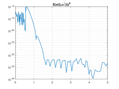
Figure 1: Test 1: Residual along the optimal trajectory with $\alpha_{0}$ (top) and with the optimal $\alpha^{*}(t)$ (bottom) in logarithmic scale.

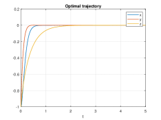
Figure 2: Test 1: Optimal trajectory with $\alpha^{*}(t)$ and initial condition $(-1,-1,-1)$

4.2 The inverted pendulum

The second example deals with the optimal control of the inverted pendulum. We denote by $x_{1}$ and $x_{3}$ as the position of the cart and its velocity, while by $x_{2}$ and $x_{4}$ the tilt angle and the corresponding velocity. Defining $x=(x_{1},x_{2},x_{3},x_{4})\in\mathbb{R}^{4}$, a possible semilinearization of the dynamics is the following

$$\dot{x}=A_{0}(x)x+g(x)x,$$

where

$$A_{0}(x)=\begin{bmatrix}0&0&1&0\\ 0&0&0&1\\ 0&a_{3,2}(x)&0&0\\ 0&a_{4,2}(x)&0&a_{4,4}(x)\end{bmatrix},$$

$$a_{3,2}(x)=m\,s(x)(\ell x_{4}-gcos(x_{2}))/c(x),$$

$$a_{4,2}=s(x)(M+m)g/(\ell c(x)),$$

$$a_{4,4}=-m\,x_{4}sin(x_{2})cos(x_{2})/c(x),$$

$$g(x)=\begin{bmatrix}0\\ 0\\ 1/c(x)\\ -cos(x_{2})/(\ell c(x))\end{bmatrix},$$

$$s(x)=sin(x_{2})/x_{2},\;c(x)=M+m\,sin(x_{2})^{2}.$$

We fix $M=0.5$, $m=0.45$, $\ell=0.5$ and $g=9.81$.

We are interested in the minimization of the following cost functional

$$J=\frac{1}{2}\int_{0}^{\infty}x^{\top}(s)Qx(s)+|u(s)|^{2}\,ds$$

where $Q=diag(1,10,0.1,0.1)$.

We are going to compare again the performance of the algorithm in absence and in presence of the optimal affine combination. We will fix $tol=10^{-9}$. First of all, let us fix the initial condition $(0,3,0,0)$. In this case the construction of the optimal trajectory using $A_{0}(x)$ fails, since the dynamics passes through points in which the couple $(A_{0}(x),g(x))$ is not stabilizable and it is not possible to solve the Riccati equation (5). However, using instead the semilinear representation

$$[\tilde{A}(x)]_{i,j}=\begin{cases}[A_{0}(x)]_{i,j}-x_{4}&(i,j)=(2,2),\\ [A_{0}(x)]_{i,j}+x_{2},&(i,j)=(2,4),\\ [A_{0}(x)]_{i,j}&otherwise\end{cases}$$

the couple $(\tilde{A}(x),g(x))$ becomes stabilizable for all the points along the trajectory. The plots of the optimal trajectories in these two cases are shown in Figure 3. In the first case the dynamical trajectory diverges at time $t=1.2$, while the latter case is able to reach the equilibrium. This illustrates that the proposed technique is able to find a stabilizing linear perturbation.

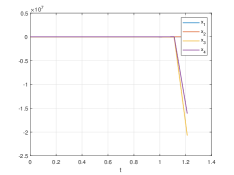
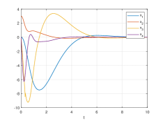
Figure 3: Test 2: Optimal trajectories with initial condition $(0,3,0,0)$ and different semilinear representations: the case with $A_{0}(x)$ (top) and the one with $\tilde{A}(x)$ (bottom).

Now let us fix the initial condition $(-0.2,-0.2,0,0)$. In this case the Riccati equations obtained using the semilinear representation formed by $A_{0}(x)$ can be solved on the optimal trajectory, allowing a comparison with the method based on the optimal affine combination. Again we notice that the introduction of the affine combination leads to a lower total residual and also to a lower total cost functional, as it can be observed by Table 2. The computation of the affine combination requires the resolution of minimization problems which leads to a slow-down of almost $8$ times. The optimal trajectory and the residual $E(x(t),\alpha(t))$ picking the optimal $\alpha^{*}$ are displayed in Figure 4. The residual presents a chattering behaviour at the beginning, due to the increase of the last two variables in the corresponding time interval. Finally we note again that as the dynamics approaches the equilibrium, the residual decays.

Semilinear form	Total cost	Total res	CPU
$A_{0}(x)$	1.29	0.25	0.3s
$\mathcal{A}(x,\alpha^{*})$	1.27	7.7e-10	2.5s

Table 2: Test 2: Comparison between the fixed and the optimal case in terms of total cost and total residual.

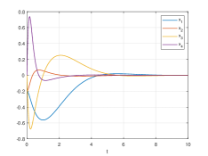
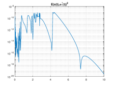
Figure 4: Test 2: Optimal trajectories with initial condition $(-0.2,-0.2,0,0)$ (top) and the residual along the trajectory (bottom) with the optimal $\alpha^{*}$ .

5 Conclusions

We presented a novel method for the resolution of optimal control problems via a SDRE approach. The choice of a fixed semilinear representation for the entire resolution of the optimal control problem using the SDRE approach may be much less accurate than the application of the original HJB equations and sometimes it may affect the asymptotic stabilization of the dynamics. In this work we proposed a systematic construction of semilinear representations obtained perturbing the entries of an initial matrix and minimizing the residual in approximating the HJB by the SDRE. The numerical tests demonstrated that the proposed method is able to achieve low orders residual and a better accuracy in terms of cost functional. Moreover in the considered tests it succeeds in finding a matrix $\mathcal{A}(x,\alpha^{*})$ such that the couple $(\mathcal{A}(x,\alpha^{*}),g(x))$ turns to be stabilizable. The choice of the optimal semilinear form would be as expensive as solving the original HJB equation. Here we propose an approach which scales polynomially in the dimension, hence it is feasible from a numerical point of view. Although the entire procedure has been presented as an online phase, an offline computation of the value function on a grid can be introduced. For instance, one may consider a data-driven approach for the construction of the value function (Albi et al. (2021); Dolgov et al. (2022)). In the future we aim at further investigating the combination of the semilinearizations and their minimization to achieve better results and their use for higher dimensional applications.

References

- Albi et al. (2021) Albi, G., Bicego, S., and Kalise, D. (2021). Gradient-augmented supervised learning of optimal feedback laws using state-dependent riccati equations. IEEE Control Systems Letters, 6, 836–841.
- Alla and Saluzzi (2020) Alla, A. and Saluzzi, L. (2020). A HJB-POD approach for the control of nonlinear PDEs on a tree structure. Applied Numerical Mathematics, 155, 192–207.
- Azmi et al. (2021) Azmi, B., Kalise, D., and Kunisch, K. (2021). Optimal feedback law recovery by gradient-augmented sparse polynomial regression. J. Machin. Learn. Res., 22(48), 1–32.
- Banks et al. (2007) Banks, H.T., Lewis, B.M., and Tran, H.T. (2007). Nonlinear feedback controllers and compensators: a state-dependent riccati equation approach. Comput. Optim. Appl., 37(2), 177–218.
- Beeler et al. (2000) Beeler, S.C., Tran, H.T., and Banks, H.T. (2000). Feedback control methodologies for nonlinear systems. J. Optim. Theory Appl., 107(1), 1–33.
- Benner and Heiland (2018) Benner, P. and Heiland, J. (2018). Exponential stability and stabilization of extended linearizations via continuous updates of riccati-based feedback. International Journal of Robust and Nonlinear Control, 28(4), 1218–1232.
- Chow et al. (2019) Chow, Y.T., Darbon, J., Osher, S., and Yin, W. (2019). Algorithm for overcoming the curse of dimensionality for state-dependent Hamilton-Jacobi equations. J. Comput. Phys., 387, 376–409.
- Cloutier et al. (1997a) Cloutier, J.R., D’Souza, C.N., and Mracek, C.P. (1997a). Nonlinear regulation and nonlinear control via the state-dependent Riccati equation technique. I. Theory. In First International Conference on Nonlinear Problems in Aviation and Aerospace (Daytona Beach, FL, 1996), 117–130. Embry-Riddle Aeronaut. Univ. Press, Daytona Beach, FL.
- Cloutier et al. (1997b) Cloutier, J.R., D’Souza, C.N., and Mracek, C.P. (1997b). Nonlinear regulation and nonlinear control via the state-dependent Riccati equation technique. II. Examples. In First International Conference on Nonlinear Problems in Aviation and Aerospace (Daytona Beach, FL, 1996), 131–141. Embry-Riddle Aeronaut. Univ. Press, Daytona Beach, FL.
- Dolgov et al. (2021) Dolgov, S., Kalise, D., and Kunisch, K. (2021). Tensor Decompositions for High-dimensional Hamilton-Jacobi-Bellman Equations. SIAM J. Sci. Comput., 43, A1625–A1650.
- Dolgov et al. (2022) Dolgov, S., Kalise, D., and Saluzzi, L. (2022). Data-driven Tensor Train Gradient Cross Approximation for Hamilton-Jacobi-Bellman Equations. arXiv preprint arXiv:2205.05109.
- Grüne and Pannek (2011) Grüne, L. and Pannek, J. (2011). Nonlinear model predictive control. Communications and Control Engineering Series. Springer, London. Theory and algorithms.
- Grüne and Rantzer (2008) Grüne, L. and Rantzer, A. (2008). On the infinite horizon performance of receding horizon controllers. IEEE Trans. Automat. Control, 53(9), 2100–2111.
- Han et al. (2018) Han, J., Jentzen, A., and E, W. (2018). Solving high-dimensional partial differential equations using deep learning. Proc. Natl. Acad. Sci. USA, 115(34), 8505–8510.
- Herty and Kalise (2018) Herty, M. and Kalise, D. (2018). Suboptimal nonlinear feedback control laws for collective dynamics. In 2018 IEEE 14th International Conference on Control and Automation (ICCA), 556–561.
- Jones and Astolfi (2020) Jones, A. and Astolfi, A. (2020). On the solution of optimal control problems using parameterized state-dependent Riccati equations. In 2020 59th IEEE Conference on Decision and Control (CDC), 1098–1103.
- Krener (2020) Krener, A.J. (2020). Al’brekht’s method in infinite dimensions. In 2020 59th IEEE Conference on Decision and Control (CDC), 5653–5658. IEEE.
- Nakamura-Zimmerer et al. (2021) Nakamura-Zimmerer, T., Gong, Q., and Kang, W. (2021). Adaptive Deep Learning for High-Dimensional Hamilton–Jacobi–Bellman Equations. SIAM J. Sci. Comput., 43(2), A1221–A1247.
- Wang and Wu (1998) Wang, J. and Wu, G. (1998). A multilayer recurrent neural network for solving continuous-time algebraic Riccati equations. Neural Networks, 11(5), 939–950.
- Çimen (2008) Çimen, T. (2008). State-dependent riccati equation (sdre) control: A survey. IFAC Proceedings Volumes, 41(2), 3761–3775. https://doi.org/10.3182/20080706-5-KR-1001.00635. 17th IFAC World Congress.