Abstract

We introduce the Correlated Preference Bandits problem with random utility based choice models (RUMs), where the goal is to identify the best item from a given pool of $n$ items through online subsetwise preference feedback. We investigate whether models with a simple correlation structure, e.g. low rank, can result in faster learning rates. While we show that the problem can be impossible to solve for the general ‘low rank’ choice models, faster learning rates can be attained assuming more structured item correlations. In particular, we introduce a new class of Block-Rank based RUM model, where the best item is shown to be $(\epsilon,\delta)$-PAC learnable with only $O(r\epsilon^{-2}\log(n/\delta))$ samples. This improves on the standard sample complexity bound of $\tilde{O}(n\epsilon^{-2}\log(1/\delta))$ known for the usual learning algorithms which might not exploit the item-correlations ($r\ll n$). We complement the above sample complexity with a matching lower bound (up to logarithmic factors), justifying the tightness of our analysis. Further, we extend the results to a more general ‘noisy Block-Rank’ model, which ensures robustness of our techniques. Overall, our results justify the advantage of playing subsetwise queries over pairwise preferences $(k=2)$, we show the latter provably fails to exploit correlation.

1 Introduction

We give an algorithm for sequentially PAC learning the best item from a finite pool of $n$ items, where at each decision round $t$, a subset of $k$ items can be tested, and preference feedback of the winning item can be observed. Given a fixed $\epsilon,\delta\in[0,1]$, the objective of the algorithm is to find, with high probability $1-\delta$, an ‘$\epsilon$-best’ item, with minimum possible query complexity.

The problem has been studied extensively in recent works in the setting of pairwise preferences (i.e. $k=2$) (Szörényi et al., 2015; Falahatgar et al., 2017; Busa-Fekete and Hüllermeier, 2014), while some works also extend the setting to general subsetwise queries (Ren et al., 2018; Saha and Gopalan, 2019; Chen et al., 2018) for specific choice of random utility model (RUM) based subset choice model (e.g. MNL or Plackett-Luce model Agrawal et al. (2016)). While at a first glance, one might expect the sample complexity of an optimal learner to depend on the sizes of the subsets queried (i.e., $k$)—precisely, with increasing subset size $k$, one may expect to achieve faster learning rates, as with larger $k$, the learner also gets to observe a preference feedback on more items per time step.

However, surprisingly, it is known that in general, the fundamental performance limit of the problem is not improvable based on the subset size $k$. For e.g., Saha and Gopalan (2018); Ren et al. (2018) formally shows a worst-case sample complexity lower bound of $O(\frac{n}{\epsilon^{2}}\log\frac{1}{\delta})$ for any $k\in[n]$ which has no dependence on $k$. These results are of course discouraging, since they imply there is no advantage in observing general subsetwise feedback over pairwise preferences ($k=2$). Why should one even build systems for general $k$-subset size queries when a pairwise query serves as good?

Our first step towards answering the above is the following crucial observation: the subset size obliviousness of the earlier results is rooted in the fact that here aforementioned results assume a no-correlations among the item rewards structure. But this in turn implies that the winning probability of a certain item in a $k$-subset solely depends on its own underlying value, and is independent of the context (rest of items present alongside), which is often unjustified in practice. In almost every real-world scenario, the items in the decision space are often correlated with interdependent utilities or losses; e.g. in movie recommendation, if a group of users dislikes a movie from the horror genre, it is likely they will dislike a thriller movie as well, similarly in restaurant recommendation, if a person shows preference for ‘tiramisu’, one may expect the similar desert items are also going to be in the top of their preference list etc. Thus depending on the nature of correlations, correlations may help in faster information aggregation where the learner can hope to gather side information about related items without explicitly learning the underlying scores (rewards) of each item separately.

Assuming ‘independent rewards’ however defeats the purpose of subsetwise games. This is since despite having the provision of playing a larger set of items (and hence observing feedback on a larger item set per round), due to the ‘independence’ assumption, the preference outcome of one item does not reveal any information of the rest as their scores remains unaffected by each other’s presence. We thus focus our attention to studying the interplay between learning rate and reward correlations in preference bandits: Here the preference information of one item can reveal additional partial preferential information of the items present alongside and hence, one can hope that selecting larger subsets in such settings should lead to faster learning rates (smaller sample complexity).

As mentioned above, to the best of our knowledge, none of the earlier work address this perspective in the setting of preference bandits, arguably due to the ease of analyzing their proposed algorithms under the ‘independent (uncorrelated)’ assumption, e.g., Saha and Gopalan (2019); Khetan and Oh (2016); Chen et al. (2018) exploit the Independence of Irrelevant Attributes (IIA) property of the Plackett Luce (PL) preference model in their sample complexity analysis. In fact, it is unclear how to incorporate ‘correlation structures’ into subsetwise preference models.

The main objective of our work is to formulate and understand how playing a subsetwise game can improve the sample complexity of the best arm identification problem for correlated items (without the learner having prior knowledge of the underlying correlation structure). Our contributions are:

(1) We introduce the problem of Correlated Preference Bandits under random utility based preference models (RUMs), which generalizes the Independent-RUM-Choice-Model  model by incorporating item correlations in terms of Low-Rank-Choice-Models LR-RUM$(n,k,r)$  (see Sec. 2 and 3).

(2). Our first finding shows that for any general Low-Rank-Choice-Model  LR-RUM$(n,k,r)$, the best-arm identification problem can be impossible to solve for (see Lem. 1, Sec. 4).

(3). We then introduce a new class of Block-Rank  based RUM model which uses a more combinatorially interpretable notion of rank. We show that in the setting of RUMs with block rank at most $r$, namely BR-RUM$(n,k,r)$  the best item is $(\epsilon,\delta)$-PAC learnable in just $O(r\epsilon^{-2}\log(n/\delta))$ samples when $k>2$ (Thm. 2, Sec. 5.1). This improves over the known sample complexity bound of $\tilde{O}(n\epsilon^{-2}\log(1/\delta))$ of the case where the arms are independent when $r\ll n$.

(4). We complement our upper bound with a matching lower bound (up to logarithmic factors), justifying the tightness of our analysis (Thm. 5, Sec 5.2).

(5). We also show a lower bound of $\Omega(n\epsilon^{-2}\log(1/\delta))$ (Thm. 6, Sec. 5) when the learner is forced to play just pairwise queries ($k=2$), which indicates how playing larger subset sizes allows the learner to exploit the underlying correlation structure achieving faster learning rates. In contrast, however, a pairwise query model $(k=2)$ fails to exploit the underlying correlation structure as shown in Thm. 5.

(6). Finally we extend our analysis to a general $\eta$-‘noisy-Block-Rank’ based RUM choice model justifying robustness of proposed method which shows its $O(r\epsilon^{-2}\log(n/\delta))$ sample complexity performance remains unaffected under some ‘tolerable $\eta$-noise’ in the correlation structure even if the underlying correlation matrix becomes full rank, i.e. $r=n$ (Sec. 6).

This work is mostly theoretical in nature and in particular has no societal impact.

Related Works. For the classical multiarmed bandits setting, there is extensive literature on PAC-arm identification problem (Even-Dar et al., 2006; Audibert and Bubeck, 2010; Kalyanakrishnan et al., 2012; Karnin et al., 2013; Jamieson et al., 2014), where the learner gets to see a noisy draw of absolute reward feedback of an arm upon playing a single arm per round. On the contrary, learning to identify the best item(s) with only relative preference information (ordinal as opposed to cardinal feedback) has seen steady progress since the introduction of the dueling bandit framework (Zoghi et al., 2013) with pairs of items (size-$2$ subsets) that can be played, and subsequent work on generalization to broader models both in terms of distributional parameters (Yue and Joachims, 2009; Gajane et al., 2015; Ailon et al., 2014; Zoghi et al., 2015) as well as combinatorial subset-wise plays (Mohajer et al., 2017; González et al., 2017; Saha and Gopalan, 2018; Sui et al., 2017).

There have been a few works in the MAB literature to exploit the advantages of item correlations, which assume the knowledge of the correlation structure (in terms of side information or online feedback-graphs). Mannor and Shamir (2011); Kocak et al. (2014, 2016); Alon et al. (2015, 2017) study the MAB problem assuming a relation graph over the nodes, however their setting also requires revealing rewards of the neighboring set of the pulled arm, which reduces this to a semi-bandit (side information) setting. On the contrary, our setting is based on a pure bandit feedback model that reveals only a noisy reward of the selected arm. Hanawal et al. (2015) also consider a stochastic sequential learning problems on graphs but here the learner gets to observe the average reward of a group of graph nodes rather than a single one. Simchowitz et al. (2016) studies the top $k$ item determination problem of multiarmed bandits for correlated arm rewards (where the underlying correlation structure can be arbitrary) and show that in the worst case the learner could be forced to consider all $\Omega\left(n\choose k\right)$ subsets. Singh et al. (2020); Gupta et al. (2019) studies the MAB regret minimization problem under correlated arms, modeling the reward dependencies in terms of clusters or some known correlation structures. To the best of our knowledge there have been no previous attempts towards understanding how item correlations affect the sample complexity of the winner determination problem in preference bandits, specifically in settings where the learner has no prior knowledge of the underlying correlation, which is the primary focus of the current work. We believe that this is a new direction which can be explored along multiple fronts.

2 Preliminaries

Notations. We denote by $[n]$ the set $\{1,2,...,n\}$.

2.1 Low Rank Subset Choice Models (accounting Item Correlations)

Before introducing our Low-Rank-Choice-Model, we recall the definition of the standard (independent) discrete random utility based choice models (RUMs) Azari et al. (2012); Chen et al. (2018) used in the preference bandits literature, which however do not take into account the item correlations.

Discrete Random Utility based Choice Model (RUMs). RUMs are a widely-studied class of discrete choice models; they assume a (non-random) ground-truth utility score $\mu_{i}\in{\mathbb{R}}$ for each alternative $i\in[n]$, and assign a distribution ${\mathcal{D}}_{i}(\cdot|\mu_{i})$ for scoring item $i$, where ${\mathbf{E}}[{\mathcal{D}}_{i}\mid\mu_{i}]=\mu_{i}$. To model a winning alternative given any set $S\subseteq[n]$, one first draws a random utility score $X_{i}\sim{\mathcal{D}}_{i}(\cdot|\mu_{i})$ for each alternative in $S$, and selects an item with the highest random score. More formally, the probability that an item $i\in S$ emerges as the winner in set $S$ is given by:

$$Pr(i|S)=Pr(X_{i}>X_{j}~{}~{}\forall j\in S\setminus\{i\}),$$ (1)

where ties are broken uniformly over all elements in set $S$. It is generally assumed that for each item $i\in[n]$, its random utility score $X_{i}$ is of the form $X_{i}=\mu_{i}+\zeta_{i}$, where all the $\zeta_{i}\sim{\mathcal{D}}$ are ‘noise’ random variables drawn independently from a probability distribution ${\mathcal{D}}$. For the purposes of analysis, it is generally assumed without loss of generality, that $\mu_{1}>\mu_{i}\,\forall i\in[n]\setminus\{1\}$ for ease of exposition. Formally, we define the best-item to be one with the highest score parameter: $i^{*}\in\underset{i\in[n]}{\text{argmax}}~{}\mu_{i}=\{1\}$, under the assumptions above. We will denote the model as Independent-RUM-Choice-Model (I-RUM$(n,k)$) for the rest of the paper.

Popular examples of I-RUM$(n,k)$. A widely used RUM is the Multinomial-Logit (MNL) or Plackett-Luce model (PL), where the ${\mathcal{D}}_{i}$’s are taken to be independent Gumbel$(0,1)$ distributions with location parameters $0$ and scale parameter $1$ (Azari et al., 2012), which results in score distributions $Pr(X_{i}\in[x,x+dx])=e^{-(x-\mu_{i})}e^{-e^{-(x-\mu_{i})}}dx$, $\forall i\in[n]$. Similarly, other different families of discrete choice models can be considered for different choices of the underlying iid noise model $\zeta_{i}\sim{\mathcal{D}}$, e.g. Exponential, Uniform, Gaussian, Weibull etc Saha and Gopalan (2020).

Limitations of existing results for I-RUM$(n,k)$. The $(\epsilon,\delta)$-PAC best-arm identification problem under this model has already been studied in the literature. In particular,  Saha and Gopalan (2018, 2020) show a fundamental sample complexity lower bound of ${\Omega}(\frac{n}{\epsilon^{2}}\ln\frac{1}{\delta})$ for this, given fixed $\epsilon,\delta\in(0,1)$. A disappointing takeaway from these results are that the bounds are subset size independent, which triggers the natural question: Why should one play subsets of larger sizes if it does not lead to a faster learning rate? One can simply get away with the problem of identifying the $\epsilon$-best item by just playing pairwise preference games $(k=2)$ in that case.

Main questions: Can we exploit reward correlations in Preference Bandits (with $k$-subsetwise pulls) without the knowledge of the underlying correlation structure? Naturally the first question is if we incorporate utility correlations in $(X_{1},\ldots X_{n})$ does that lead to faster learning rate? Further, what is the right measure of correlation in a choice model?

Remark 1 (Why MAB setup can not exploit reward correlations).

Note in the setting of standard MAB, the item correlations do not play any role in improving the learning rate beyond $\Omega(\frac{n}{\epsilon^{2}}\ln\frac{1}{\delta})$ Even-Dar et al. (2006). This is due to the inherent limitation of models which restrict the learner to query feedback of just single arms at every round – this means irrespective of the correlation model $\Sigma$, the learner would never have a way to distinguish if two arms are fully correlated or exactly identical from single arm pulls.

Our proposed preference-choice models (to capture correlations). Towards this we study the following natural generalization of I-RUM$(n,k)$: Define the utility score vector $X$ as a multivariate random variable of the form: $X={\boldsymbol{\mu}}+\boldsymbol{\zeta}$, where $\boldsymbol{\zeta}\sim{\mathcal{D}}$ is a multivariate noise drawn from a joint distribution ${\mathcal{D}}$ (instead of sampling the $n$ utility scores $X=(X_{1},\ldots,X_{n})$ independently), such that it has mean zero and correlation structure quantified by the $n\times n$-matrix of correlation coefficients $\Sigma:={\rm Corr}(\boldsymbol{\zeta})$. Again, the choice probability $P(i|S)$ of any arm $i\in S$ in any subset $S\subseteq[n]$, can still be defined same as that suggested in Eqn. (1). We refer to this model as Correlated-RUM-based-Choice-Models. For example, assume ${\mathcal{D}}={\mathcal{N}}({\mathbf{0}},\Sigma)$—a multivariate zero mean Gaussian noise with some fixed (but unknown) covariance matrix $\Sigma$. In particular when $\Sigma$ is not the identity matrix, this recovers a ‘correlated Gaussian based choice model’.

Low-Rank-Choice-Model (LR-RUM$(n,k,r)$). A first step towards understanding the effect of item correlations on learning rate is to determine a suitable ‘measure of correlation’ among the utility scores $X_{1},\ldots,X_{n}$ in terms of some properties of the underlying correlation matrix $\Sigma$. Formally $\Sigma$ is a $n\times n$ matrix such that $\Sigma(i,j):={\rm Corr}(\zeta_{i},\zeta_{j})$ where ${\rm Corr}(\cdot,\cdot)$ is used to denote the correlation coefficient. A natural quantity to express the complexity of item correlations is the rank of the underlying correlation matrix. E.g. PCA (Bishop (2006)) or Matroids (Oxley (2006)) which has varied applications in many real systems including image, graph networks or information retrieval. Motivated by these, we define the Low-Rank-Choice-Model, which models the item dependencies through rank of the correlation matrix $\Sigma$. Precisely we assume ${\texttt{Rank}}(\Sigma)=r$ for some $r\in[n]$. Clearly the setting $r=n$ expresses independent discrete RUM based choice model as a special case. We will henceforth denote this model by ‘$r$-Low-Rank-Choice-Model’ or LR-RUM$(n,k,r)$.

$r$-Block-Rank. An interesting special case of low-rank choice model is one where the item correlations results in an $r$-clustering (referred to as ‘blocks’ henceforth) of the set of items. In particular, we say that a $r$-Block-Rank  instance has block-rank $r$ if there exists a partitioning on the set of items $[n]$ into blocks ${\mathcal{B}}_{1}\uplus{\mathcal{B}}_{2}\uplus\cdots\uplus{\mathcal{B}}_{r}$ such that the following properties hold:

• Inter-block Identity: For any block ${\mathcal{B}}_{i}$ and any pair of items $a,b\in{\mathcal{B}}_{i}$, we have $\zeta_{a}=\zeta_{b}$.

• Cross-block Independence: For any subset of items $S\subseteq[n]$ such that $|S\cap{\mathcal{B}}_{i}|\leq 1$ for every $i\in[r]$, the set of variables $(\zeta_{i})_{i\in S}$ is jointly independent.

Note that in this setting, the correlation matrix admits a block diagonal structure i.e.,

$$\Sigma(a,b)=\begin{cases}1,~{}\forall a,b\in{\mathcal{B}}_{i},~{}i\in[r],\\ 0,~{}\forall a\in{\mathcal{B}}_{i},b\in{\mathcal{B}}_{j},~{}i,j\in[r],~{}i\neq j.\end{cases}$$

Again for brevity, we shall refer to this model as BR-RUM$(n,k,r)$  in the rest of the paper.

(Noisy) $(r,{\tilde{\eta}},\eta)$-Block-Rank. The $(r,{\tilde{\eta}},\eta)$-Block-Rank model generalizes $r$-Block-Rank by allowing intra-block variables to be almost correlated and inter-block variables to be nearly independent (for some ${\tilde{\eta}},\eta\in(0,1]$). Formally, in $(r,{\tilde{\eta}},\eta)$-Block-Rank instance, the set of items $[n]$ admits a partitioning into blocks ${\mathcal{B}}_{1}\uplus\cdots\uplus{\mathcal{B}}_{r}$ such that the following properties hold.

• Cross-block Approximate Independence: For any subset of items $S\subseteq[n]$ such that $|S\cap{\mathcal{B}}_{i}|\leq 1$ and any non-trivial partitioning $S=S_{1}\uplus S_{2}$ we have $I(\zeta_{S_{1}};\zeta_{S_{2}})\leq{\tilde{\eta}}$ where $\zeta_{S_{1}}:=(\zeta_{i})_{i\in S_{1}}$ denotes the set of variables in $S_{1}$ and $I(\cdot,\cdot)$ denotes the mutual information (MI) between two (sets of) variables.

• Inter-block Approximate Identity: For any block ${\mathcal{B}}_{i}$ and any pair of items $a,b\in{\mathcal{B}}_{i}$ we have ${\rm Corr}(\zeta_{i},\zeta_{j})\geq 1-\eta$.

Note that instantiating ${\tilde{\eta}},\eta=0$, we recover the $r$-Block-Rank setting as a special case. For Gaussian noise, one can express both items (i) and (ii) above in terms of correlation, since it is folklore that a pair of Gaussians can be uncorrelated if and only if they are independent.

3 Problem Setting

We consider the Probably Approximately Correct (PAC) version of the best-arm identification problem through subset-wise comparisons. Formally, the learner is given a finite set $[n]$ of $n>2$ items or ‘arms’ along with a playable subset of size $k\leq n$. At each round $t=1,2,\ldots$, the learner selects a subset $S_{t}\subseteq[n]$ of size at most $k$ distinct items, and receives (stochastic) feedback of the ‘winning item’ drawn according to $Pr(\cdot\mid S_{t})$ (see Eqn. (1)) depending on (a) the chosen subset $S_{t}$, and (b) a LR-RUM$(n,k,r)$  choice model with parameters ${\boldsymbol{\mu}}=(\mu_{1},\mu_{2},\ldots,\mu_{n})$ a priori unknown to the learner.

3.1 Correctness and Sample Complexity: $(\epsilon,\delta)$-PAC arm identification in LR-RUM

For a Low-Rank-Choice-Model  LR-RUM$(n,k,r)$  instance with $n\geq k$ arms, an arm $i\in[n]$ is said to be $\epsilon$-optimal if $\mu_{i}>\mu_{1}-\epsilon$. A sequential learning algorithm that depends on feedback from an appropriate subset-wise feedback model is said to be $(\epsilon,\delta)$-PAC, for given constants $0<\epsilon\leq\frac{1}{2},0<\delta\leq 1$, if the following properties hold when it is run on any instance LR-RUM$(n,k,r)$: (a) it stops and outputs an arm $I\in[n]$ after a finite number of decision rounds (subset plays) with probability $1$, and (b) the probability that its output $I$ is an $\epsilon$-optimal arm in LR-RUM$(n,k,r)$  is at least $1-\delta$, i.e, $Pr(\text{$I$ is $\epsilon$-optimal})\geq 1-\delta$. By sample complexity of the algorithm, we mean the expected time (number of decision rounds) taken by the algorithm to stop when run on the instance LR-RUM$(n,k,r)$.

4 Impossibility Result: General Low-Rank-Choice-Model

In this section we show that allowing for arbitrary correlations can make the $\epsilon$-optimal winner determination problem ill defined in the following sense: one can construct instances where there are subsets for which the item with the largest win probability is not the same as the item with the largest score. In particular, such instances can be simply constructed in a way such that the covariance matrix is just $2$-dimensional. We state the observation formally in the following lemma.

Lemma 1.

Consider an instance of LR-RUM$(n,k,r)$  with $n=k$, and $r=2$. Then for any even $k\geq 4$ and $0<\epsilon\leq\epsilon(k)$, there exist scores $\mu_{1}>\mu_{2}+\epsilon\geq\cdots\geq\mu_{k}$ with underlying correlation matrix $\Sigma\in{\mathbb{R}}^{k\times k}$ s.t. $\operatorname*{argmax}_{i\in[k]}\operatorname*{Pr}\left(i|[k]\right)\neq 1;$ i.e. Item-$1$, despite of being the only $\epsilon$-optimal item, would not have the maximum winning probability when played in a subset.

Clearly, the above kind of instances are a structural barrier (as opposed to an information theoretic one) to the winner determination problem, since if the instance itself is the subset equipped with the distribution from the above lemma, the observations will be guided by the win probabilities, which do not favor the true winner.

Proof Sketch of Lem. 1.

Consider the following generic way of constructing a family of correlated Gaussians using unit vectors ${\bf v}_{1},\ldots,{\bf v}_{k}$. (i). Sample a random Gaussian vector ${\bf g}\sim{\mathcal{N}}({\bf 0},{\bf I}_{2\times 2})$. (ii). For every $i\in[k]$, set $g_{i}=\langle{\bf v_{i}},{\bf g}\rangle$.

We use the above geometric interpretation to define the correlation structure of the Gaussians. For every $i\in[k]$, we set ${\bf v}_{i}:={\bf u}(\alpha_{i})$, where ${\bf u}(\alpha)$ is the unit vector $(\cos\alpha,\sin\alpha)$. We define the corresponding $\alpha_{i}$’s as follows. We set $\alpha_{1}=0$, $\alpha_{k}=\pi$ and for every $i\in\{2,\ldots,k-1\}$, we set $\alpha_{i}=(-1)^{i~{}{\rm mod}~{}2}\cdot\pi/4$.

Finally, we assign the score vector ${{\boldsymbol{\mu}}}=(\mu_{1},\ldots,\mu_{k})$ as follows. We set $\mu_{1}=\mu+\epsilon$ and $\mu_{j}=\mu$ for every $j\in[k]\setminus\{1\}$. Note that in the above construction of $(g_{1},\ldots,g_{k})$, the correlation matrix $\Sigma$ is exactly ${\bf V}^{\top}{\bf V}$ where ${\bf V}:=[{\bf v}_{1},\ldots,{\bf v}_{k}]$. Since ${\bf v}_{i}$ are $2$-dimensional unit vectors, we have ${\rm rank}(\Sigma)\leq 2$. Furthermore, arm $1$ is the only $\epsilon/2$-best arm in the setting.

Analysis. We first observe that when $\epsilon=0$ (i.e., all items are assigned score $\mu$), the win probability of an item $i$ when $[k]$ is played is exactly the angular measure of arc consisting of the points on the unit circle closest to vector ${\bf v}_{i}$. In that case, one can easily verify that

$$\operatorname*{Pr}_{{{\boldsymbol{\mu}}}^{\prime}=(\mu,\ldots,\mu)}\left(1|[k]\right)=1/8\text{ and }Pr_{{{\boldsymbol{\mu}}}^{\prime}=(\mu,\ldots,\mu)}\left(k|[k]\right)=3/8$$

Furthermore, even when $\epsilon$ is non-zero but small enough as a function of $k$, using a first order approximation argument, for the actual score vector ${{\boldsymbol{\mu}}}=(\mu+\epsilon,\mu,\ldots,\mu)$, we have the following win probability bounds: $\operatorname*{Pr}_{{{\boldsymbol{\mu}}}=(\mu+\epsilon,\ldots,\mu)}\left(1|[k]\right)\leq 1/8+o(1),~{}\operatorname*{Pr}_{{{\boldsymbol{\mu}}}=(\mu+\epsilon,\ldots,\mu)}\left(k|[k]\right)\geq 3/8-o(1)$

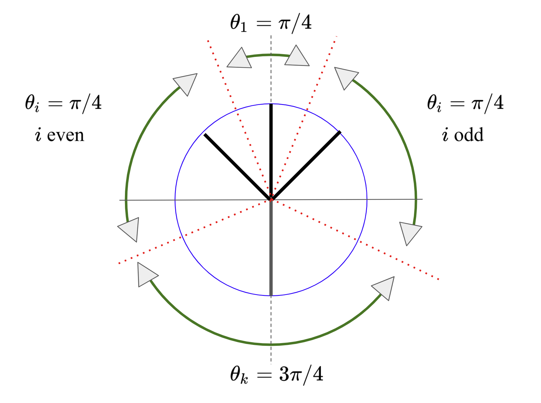
Figure 1: Winning Sectors corresponding to the arms

In summary, we have $\mu_{1}>\mu_{k}+\epsilon/2$ but $\operatorname*{Pr}(1|[k])<\operatorname*{Pr}(k|[k])$, which establishes the guarantees claimed. We include the full proof in Appendix A. ∎

5 $r$-Block-Rank  Choice Model

The impossibility result for the general Block-Rank  case (Sec. 4) motivates us to understand if a faster learning rate can be achieved through imposing more structured item correlations. In particular, in this section, we use a more combinatorial notion of measure of simplicity (namely, block rank) to explore $r$-Block-Rank  instances (see Sec. 2 for description). In particular, our contributions include an $O(r\epsilon^{-2}\log(n/\delta))$-sample complexity algorithm for PAC learning for BR-RUM$(n,k,r)$ instances when the learning algorithms is allowed to play subsets of sizes at least $3$, and complement it with matching sample complexity lower bound for the same setting. In addition, we show a $\Omega(n\epsilon^{-2}\log(1/\delta))$-sample complexity lower bound for these instance when the learner is restricted to play just pairwise duels.

5.1 Algorithm: Sample Complexity Bound

We first design an algorithm for this setup based on the following key intuition. For any instance with block rank $r$, the information theoretic bottleneck here is the winner determination problem among the best item from each of the $r$-blocks. However, the challenge here is the obvious one, the identities of these items are not known upfront, and as such, any off-the-shelf algorithm for the $(\epsilon,\delta)$-PAC learning problem which does not exploit the underlying correlation structure, would essentially end up solving the winner determination problem on $n$-arms leading to a sample complexity of $O(n/\epsilon^{2}\log 1/\delta)$.

Main ideas: We circumvent these issues by:

$(1)$ Fast Pre-processing step (with number of arm pulls independent of $\epsilon$) which reduces the effective pool of candidate items to a subset of size at most $r$: The pre-processing step is based on the following principle. Given any non “strictly optimal” item $i$ within a block, we can always find another item $i^{\prime}$ in the same block whose win probability is at least as large as that of $i$ on any subset $S$ which simultaneously contains $i$ and $i^{\prime}$. On the other hand, since $1$ is the unique winner, it’s win probability is never dominated by that of another item. This observation is the core guiding principle for our design of the pre-processing step which plays all possible triples and eliminates items based on their worst case win probability estimates. In particular, with high probability it returns a set of at most $r$-arms, say $S$, each of which belongs to a distinct block, and one of which is the optimal arm. Since they come from the $r$ distinct blocks, they are independent.

$(2)$ Now to obtain an $\epsilon$-best item, we simply run the Sequential-Pairwise-Battle algorithm of Saha and Gopalan (2020) (precisely Seq-PB$(S,\min(k,r),\epsilon,\delta/2,c({\mathcal{D}}))$, which is known to be a provably optimal $(\epsilon,\delta)$-PAC for any I-RUM$(n,k)$  given any underlying noise model distribution ${\mathcal{D}}$ ($c({\mathcal{D}})$ being a constant depending on the ‘minimum-Best-Item-Advantage-Ratio’ ($\epsilon$-BAR) of ${\mathcal{D}}$, see Defn. 7). Note that our algorithm is adaptive and does not require prior knowledge of the block-rank $r$. The pseudocode is given as Algorithm 1.

Algorithm 1 Block-Rank Preference Bandits  (BlockRank-PB)

1:  Input:

2:      Set of items: $[n]$. Error bias: $\epsilon>0$, Confidence parameter: $\delta>0$.

3:      Noise model $({\mathcal{D}})$ (or equivalently $c({\mathcal{D}})$, a noise model dependent constant)

4:  Initialize:

5:      $t\leftarrow O\left(\log\frac{4n^{3}}{\delta}\right)$ and set ${\rm Flag}(i)\leftarrow 0$ for every $i\in[n]$.

6:  for ${\mathcal{T}}\in{[n]\choose 3}$ do

7:         Play the triple ${\mathcal{T}}$ for $t$-times. For $i\in{\mathcal{T}}$, let $N_{\mathcal{T}}(i)$ be the number of times $i$-wins.

8:         For every item $i\in{\mathcal{T}}$ such that $N_{{\mathcal{T}}}(i)\leq 0.26t$, mark ${\rm Flag}(i)\leftarrow 1$.

9:  end for

10:      Construct set $S:=\{i\in[n]|{\rm Flag}(i)=0\}$.

11:      Find: $\hat{i}\leftarrow$ Seq-PB$(S,\min(k,|S|),\epsilon,\delta/2,c({\mathcal{D}}))$ (Alg. 1, Saha and Gopalan (2020)).

12:      Output $\hat{i}$: The winner returned by Seq-PB.

The following theorem formally states the guarantee of the above algorithm.

Theorem 2 (Alg. 1: Correctness and Sample Complexity for BR-RUM$(n,k,r)$).

Consider any BR-RUM$(n,k,r)$  Block-Rank  choice model with noise distribution ${\mathcal{D}}$, $k>2$. Then, Alg. 1 is $(\epsilon,\delta)$-PAC with sample complexity $\max\left\{O(n^{3}\log(n/\delta)),O(\frac{r}{c\epsilon^{2}}\ln\frac{r}{\delta})\right\}$, where $c:=c({\mathcal{D}})$ is a constant depending on ${\mathcal{D}}$.

Remark 2 (Improved Sample Complexity).

Note that above implies improved sample complexity of $O(r\epsilon^{-2}\log(r/\delta))$ which is much smaller than the usual bound of $O(n\epsilon^{-2}\log(r/\delta))$, when $r\ll n$. This is due to the fact that in general, block rank is a more precise notion of the effective number of arms to be considered for the winner determination problem.

Remark 3 (Parameter regime for improved Sample Complexity).

The above algorithm exhibits improved sample complexity $O(r\epsilon^{-2}\log(n/\delta))$ for all $\epsilon\in(0,(r/n^{3})^{1/2}]$; this improves on the $O(n\epsilon^{-2}\log(n/\delta))$ of Saha and Gopalan (2020) for the I-RUM$(n,k)$ model. In particular, we don’t need $n$ to be constant for the overall sample complexity to be $O(r\epsilon^{-2}\log(r\delta))$ i.e., it is actually the trade-off between $r/n$ and $\epsilon$ that determines the regime of parameters under which Algorithm 1 exhibits improved convergence rates.

Remark 4.

In particular, Saha and Gopalan (2020) show that $c({\mathcal{D}})$ is a constant for several popular choices of noise distributions such as Uniform, Gumbel, Gaussian, Gamma, Weibull (see). Consequently, our algorithm Block-Rank Preference Bandits  gives a $O(\frac{r}{\epsilon^{2}}\log(n/\delta))$-sample complexity guarantee for all such distributions as shown in the Thm. 2.

Proof Sketch of Thm. 2.

Justifying Correctness. It is based on the following idea that when items are played in triples, there exists a separation in worst case win-probabilities (when played in triples) between non-strictly optimal items and the best item.

Claim 1.

For any triple ${\mathcal{T}}=(1,i,j)$, we have $Pr(1|{\mathcal{T}})\geq 1/3$.

Claim 2.

For any triple ${\mathcal{T}}=(1,i,j)$, such that $i,j$ are from the same block, if $\mu_{i}\geq\mu_{j}$, then $\operatorname*{Pr}\left(j|{\mathcal{T}}\right)\leq 1/4$.

The first two claims taken together imply: (a) every item $j$ whose score $\mu_{j}$ is not uniquely largest in its block participates in a triple where it wins with probability at most $1/4$ and (b) in every triple the best item $1$ wins with probability at least $1/3$. Since our choice of number of trials $t$ is large enough, we know that the empirical estimates are close enough approximates of the true win probabilities; points (a) and (b) also hold for the empirical win-probability estimates $\{N_{\mathcal{T}}(i)/t\}_{i,{\mathcal{T}}}$. This observations are stitched together in the following lemma which gives useful characterization of items which are flagged inside the for loop.

Lemma 3.

With probability at least $1-\delta/2$, the following holds. For any item $j\in[n]$, if there exists an item $i$ from the same block for which $\mu_{i}\geq\mu_{j}$, we have ${\rm Flag}(j)=1$. Furthermore, ${\rm Flag}(1)=0$.

In particular, with high probability, every item $j$ satisfying the premise of (b) gets flagged, whereas item $1$ never gets flagged. And whenever this high probability event holds, the resulting set $S$ must consist of at most $r$-arms, which are all independent and $1\in S$.

Lemma 4 (Pre-processing Step Guarantee).

With probability at least $1-\delta/2$, the set $S$ satisfies the following conditions. For every $i\in[r]$, $|S\cap{\mathcal{B}}_{i}|\leq 1$. Additionally $1\in S$.

Now assume that the subset $S$ satisfies the guarantees of the above lemma. Since the items in $S$ come from distinct blocks, the corresponding arms are independent and the subset-wise feedback on subsets of $S$ follow the independent RUM model. Hence running Algorithm 1 from Saha and Gopalan (2020) will return an $\epsilon$-best arm in $O(r\epsilon^{-2}\log(r/\delta))$-samples.

Justifying the Sample complexity. In the for loop (Lines 6-9), each triple ${\mathcal{T}}\in{n\choose 3}$ is played $t$ times. Therefore, then total number of arm pulls in the for loop is bounded by $O(n^{3}t)\leq O(n^{3}\log(n/\delta))$ which is a constant independent of $\epsilon$. Therefore, step corresponding to Line $11$ incurs a sample complexity cost of $O(r{\epsilon^{-2}}\log(r/\delta))$. Since the latter term dominates as $\epsilon\to 0$, this establishes the desired sample complexity. The complete proof is given in Appendix B. ∎

Remark 5.

We consider playing subsets of various sizes, because without this relaxation, the winner determination problem can again become ill defined in the correlated setting (see Lem. 17).

5.2 $r$-Block-Rank: Lower Bound

Our lower bound analysis is based on the following intuition: Given an instance ${\mathcal{I}}$ with $r$-Block-Rank, where $[n]=\uplus_{i\in[r]}{\mathcal{B}}_{i}$ is the partitioning of arms into block structure. Consider the set ${\mathcal{S}}$ constructed by adding the arm with the highest score from each block ${\mathcal{B}}_{i}$. Now the key insight is that any algorithm which solves the $\epsilon$-best arm identification problem on ${\mathcal{I}}$ must also solve the $\epsilon$-best arm identification problem on the set of independent arms ${\mathcal{S}}$. This observation can be used to embed instances of IND-RUM$(r,k,{\boldsymbol{\mu}})$ into instances of BR-RUM$(n,k,r,{\boldsymbol{\mu}}^{\prime})$, thus forcing the worst case sample complexity of the latter to be lower bounded by that of the former, which is known to be $\Omega(r\epsilon^{-2}\log(1/\delta))$.

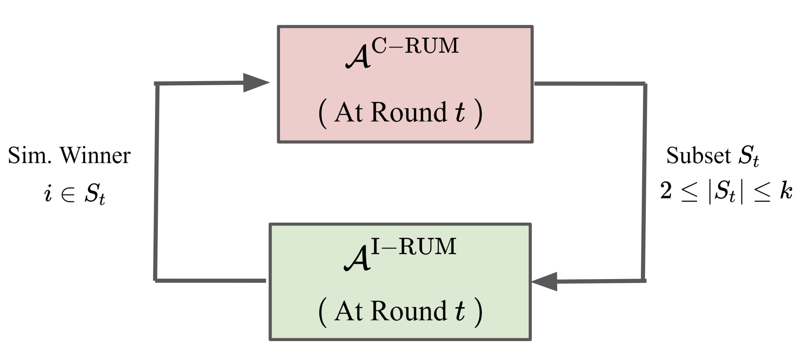
Figure 2: Reduction (Pseudocode in Appendix C.1)

Theorem 5 (Performance limit for Ordered Block-Rank).

Given $\epsilon\in(0,1]$, $\delta\in(0,1]$, $r,k\in[n]$, for any $(\epsilon,\delta)$-PAC algorithm $A$ for the $(\epsilon,\delta)$-PAC arm identification in LR-RUM, there exists an instance of BR-RUM$(n,k,r)$, say $\nu$, where the expected sample complexity of $A$ on $\nu$ is at least $\Omega\big{(}{r}\epsilon^{-2}\log 1/\delta\big{)}$.

Proof sketch of Thm. 5.

The proof of Theorem 5 uses a reduction from the problem of $(\epsilon,\delta)$-PAC learning in an IND-RUM$(r,k,{\boldsymbol{\mu}})$ instance to an $(\epsilon,\delta)$-PAC learning problem in a BR-RUM$(n,k,r,{\boldsymbol{\mu}}^{\prime})$ instance. Formally, the reduction proceeds as follows. Given an algorithm ${\mathcal{A}}^{C-RUM}$ which $(\epsilon,\delta)$-PAC learns best items from BR-RUM$(n,k,r,{\boldsymbol{\mu}}^{\prime})$ instances, we can construct an algorithm ${\mathcal{A}}^{\rm I-RUM}$ which does the same for the independent setting with $r$-arms. In particular, the algorithm embeds the best item learning problem on $r$-arms over a unknown score profile ${\boldsymbol{\mu}}$ inside best item learning problem on $n$-arms with correlations, and then uses ${\mathcal{A}}^{\rm C-RUM}$ to solve the large problem. This is done using a simple idea: the outer algorithm ${\mathcal{A}}^{\rm C-RUM}$ adds $n-r$ dummy items to the set with score $\mu_{i}=-\infty$ with appropriate correlation structure. This ensures that: (i) The $\epsilon$-best item set in $[r]$ is also the $\epsilon$-best item set in the larger set $[n]$. (ii) The algorithm ${\mathcal{A}}^{\rm I-RUM}$ can simulate the subsetwise preference feedback required by ${\mathcal{A}}^{\rm C-RUM}$ on $[n]$ using its own preference feedback on subsets of $[r]$ (Fig. 2).

Overall, if ${\mathcal{A}}^{\rm C-RUM}$ is an $(\epsilon,\delta)$-PAC algorithm for BR-RUM$(n,k,r,{\boldsymbol{\mu}}^{\prime})$, then so is ${\mathcal{A}}^{\rm I-RUM}$ for IND-RUM$(r,k,{\boldsymbol{\mu}})$. Therefore the sample complexity of ${\mathcal{A}}^{C-RUM}$ is bounded by that of ${\mathcal{A}}^{I-RUM}$, which we prove to be $\Omega(r\epsilon^{-2}\log(1/\delta))$–this is done by extending previous known lower bounds for fixed subset sizes to the setting of variable-sized subsetwise plays (Thm. 15, Appendix C.5). The proof is given in Appendix C. ∎

On the other hand, our next result shows that, there is no advantage in querying pairwise-feedback $(k=2)$ even for any $r\geq 2$ (note $r=1$ is a trivial case), as stated formally in the following theorem.

Theorem 6 (Pairwise Preferences: Sample Complexity Lower Bound for Low-Rank-Choice-Model).

Given $\epsilon\in(0,1/4]$, $\delta\in(0,1]$, and general $r\in[n]$ $(r>1)$, for any $(\epsilon,\delta)$-PAC algorithm $A$ for $(\epsilon,\delta)$-PAC arm identification in LR-RUM  problem, $\exists$ an instance of BR-RUM$(n,2,r,{\boldsymbol{\mu}})$, where the expected sample complexity of $A$ is at least $\Omega\big{(}\frac{n}{\epsilon^{2}}\log\frac{1}{\delta}\big{)}$– independent of $r$.

Remark 6 (Separation in the sample complexity for $k=2$ vs $k=3$).

Intuitively, triples can be used to determine whether a subset involves the winner much faster: Consider the instance with $2$ blocks, where the first block is a singleton with score $\mu+\epsilon$ and the second block consists of $(n-1)$.identical arms, each with score $\mu$. Then for every distinct choice of $i,j\in[n]$ we have $\operatorname*{Pr}(i|\{i,j\})=\frac{1}{2}+O(\epsilon)$ if $i=1$ and $\operatorname*{Pr}(i|\{i,j\})=\frac{1}{2}$ if $i\neq 1$ i.e, the duels involving the winner behave near identically to duels not involving it and it would take $\Omega_{\delta}(\epsilon^{-2})$-queries to distinguish between the two cases. On the other hand, consider a triple ${\mathcal{T}}:=(i,j,k)$ such $i<j<k$. Then the win probabilities for the the arms playing ${\mathcal{T}}$ are $(1/2,1/4,1/4)$ if $i=1$, and $(1/3,1/3,1/3)$ otherwise, and it would take only $O_{\delta}(1)$-queries to distinguish between the two, which is significantly smaller than that of the dueling feedback setting.

6 $(r,{\tilde{\eta}},\eta)$-Block-Rank: Algorithm and Analysis for the general Block-Rank  Choice Model under Noise

Interestingly, our findings show that even for the noisy settings, Algorithm 1 is a correct $(\epsilon,\delta)$-PAC algorithm when the correlation matrix nearly has a $0$-$1$-block diagonal structure (Thm. 13). Formally, our main results are stated as Thm. 10 and 12 which gives the precise dependence on noise-vs-the suboptimality gap and its trade-off with learning rate.

6.1 At most ${\tilde{\eta}}$-MI: Analysis for nearly-independent I-RUM$(n,k)$  model

In this section we discuss the setting of noisy-block rank model such that items across the blocks are at most “${\tilde{\eta}}$-identical” (precisely at most ${\tilde{\eta}}$-mutual information):

${\tilde{\eta}}$-I-RUM$(n,k)$: This is a generalization of I-RUM$(n,k)$  model where the noise distributions ${\mathcal{D}}_{i}$’s are no longer independent, but can have at most ${\tilde{\eta}}$-mutual information, i.e. Corr$(\zeta_{i},\zeta_{j})\leq{\tilde{\eta}}$, for any pair of distinct arms $i,j\in[n]$ (for any ${\tilde{\eta}}\in[0,1)$). Clearly, setting ${\tilde{\eta}}=0$, we recover the original I-RUM$(n,k)$  models, as studied in Saha and Gopalan (2018, 2020); Soufiani et al. (2014).

The main result of this subsection is to show that under ‘low noise’ $(\tilde{\eta})$, our algorithm BlockRank-PB  (Alg. 1) still finds an $\epsilon$-best item with $O(r\epsilon^{-2}\log(n/\delta))$ sample-complexity. Specifically, the important aspect we note is while the guarantees of Seq-PB sub-routine of Alg. 1 rely on the independence structure across blocks, it can be shown to yield correct results even under ${\tilde{\eta}}$-I-RUM$(n,k)$(Thm. 10) model under a separation of scores assumption (see Thm. 10). Before stating Thm. 10, we find it useful to introduce some definitions:

Definition 7 (Best-Item-Advantage-Ratio).

Given any I-RUM$(n,k)$  model, and subset $S\subseteq[n]$, the advantage ratio of the best item of set $S$, $i^{*}_{S}:=\operatorname*{argmax}_{i\in S}\mu_{i}$, over any other item $j\in S\setminus\{i^{*}_{S}\}$ is defined as Best-Item-Advantage-Ratio$(j,S)$:

$$\text{BAR}_{\otimes_{\ell\in[n]}{\mathcal{D}}_{\ell}}({\mathcal{I}})(j,S)=\frac{Pr(i^{*}_{S}|S)}{Pr(j|S)}.$$

(Explicit use of the subscript ${\otimes_{\ell\in[n]}{\mathcal{D}}_{\ell}}({\mathcal{I}})$ represents the underlying I-RUM$(n,k)$  model.)

Corollary 8.

It is easy to note that by definition, BAR$(j,S)>\frac{1}{kPr(j|S)}$ for any subset $S$ of size $k$, since the win probability of the best item $i_{S}^{*}$ in $S$ is at least $\frac{1}{k}$.

Definition 9 (Minimum Best-Item-Advantage-Ratio).

The $\epsilon$-Best-Item-Advantage-Ratio, ($\epsilon$-BAR), is defined to be the minimum (worst case) Best-Item-Advantage-Ratio  an $\epsilon$-best item gets against an non-$\epsilon$ best item $(j)$ globally, irrespective of which set it appears inside. More precisely, let $[n]_{\epsilon}:=\{i\in[n]\mid\mu_{i}>\mu_{1}-\epsilon\}$ denotes the set of all $\epsilon$-best items in $[n]$, then for any I-RUM$(n,k)$  model ${\mathcal{I}}$, we define its $\epsilon$-BAR$({\mathcal{I}})$  to be:

$$\text{{\it$\epsilon$-BAR}}_{\otimes_{\ell\in[n]}{\mathcal{D}}_{\ell}}({\mathcal{I}})=$$

$$\min_{S\in\{S\mid S\cap[n]_{\epsilon}\neq\emptyset\},j\in S\setminus[n]_{\epsilon}}\text{BAR}_{\otimes_{\ell\in[n]}{\mathcal{D}}_{\ell}}({\mathcal{I}})(j,S).$$ (2)

Note $\epsilon$-BAR  is a measure of worst-case quality separation of an $\epsilon$-best item over a non $\epsilon$-best item (in terms of item-preferences), which is the key complexity factor in the sample complexity analysis of Seq-PB subroutine used in Alg. 1 as stated below:

Theorem 10 (Correctness and Sample Complexity of Seq-PB on ${\tilde{\eta}}$-I-RUM$(n,k)$).

Consider any subsetwise preference model I-RUM$(n,k)$  ${\mathcal{I}}$ on the underlying noise distribution ${\mathcal{D}}$, such that $\epsilon$-BAR$({\mathcal{I}})\geq 1+\frac{4c\epsilon}{1-2c}$ for some ${\mathcal{D}}$-dependent constant $c=c({\mathcal{D}})>0$. Then Seq-PB$(n,k,\epsilon,\delta,c)$ is an $(\epsilon,\delta)$-PAC algorithm on any instance $\nu$ of ${\tilde{\eta}}$-I-RUM$(n,k)$  model with sample complexity $O(\frac{n}{c^{2}\epsilon^{2}}\log\frac{k}{\delta})$, for any ${\tilde{\eta}}<[0,\frac{c^{2}\epsilon^{2}}{32^{2}k^{4}}\big{)}$. Here $\nu$ being an instance of the I-RUM$(n,k)$  model corresponding to the noise distribution ${\mathcal{D}}$.

Proof sketch of Thm. 10.

The proof depends on the following main lemma which ensures if the $\epsilon$-BAR  of any I-RUM$(n,k)$  based preference model is bounded away by a certain threshold, then the $\epsilon$-BAR  of the corresponding ${\tilde{\eta}}$-I-RUM$(n,k)$  model will also be bounded away by nearly a same threshold for ‘small’ ${\tilde{\eta}}$.

Lemma 11 (Lower bound for the advantage ratio ${\tilde{\eta}}$-I-RUM$(n,k)$  model).

Consider I-RUM$(n,k)$  model of Thm. 10. Then for any ${\tilde{\eta}}$-I-RUM$(n,k)$  based subsetwise preference model, say ${\mathcal{I}}^{\prime}$, we have

$$\text{{\it$\epsilon$-BAR}}_{{\mathcal{D}}}({\mathcal{I}}^{\prime})\geq 1+\frac{2c\epsilon}{1-2c}.$$

Given the above lemma, the rest of the argument follows same as Thm. $4$ of Saha and Gopalan (2020) as it pivots on the main assumptions on $\epsilon$-BAR$({\mathcal{I}})$ as achieved in Lem. 11. The complete proof of Lem. 11 and Thm. 10 is given in Appendix E.1. ∎

6.2 At least $(1-\eta)$-Correlation: Nearly-identical intra-block noise

In this subsection we discuss the setting of noisy intra block items when items inside the block are almost identical, with at least $(1-\eta)$-correlation. Our main finding here is to show that the pre-processing step of BlockRank-PB  (Alg. 1), which exploits the intra-block item-correlations, is robust under ‘mild-noise’ $\eta$ or more precisely when they are at least $(1-\eta)$-correlated.

Theorem 12.

Let $\eta\in\big{[}0,\min\{\frac{1}{192},\min_{j\neq 1}\Delta^{4}_{1j}/16\}\big{]}$. Then with probability at least $1-\delta/2$, the pre-processing step (Lines $6$-$10$) constructs a set $S$ of size at most $r$ such that (i) $1\in S$ and (ii) $|S\cap{\mathcal{B}}_{a}|\leq 1$ for every $a\in[r]$. Furthermore, the number of samples queried in the pre-processing step is at most $O(n^{3}\log n/\delta)$.

We defer the proof of the above to Appendix E.2.

Remark 7.

Thm. 12 says that we need $\eta$ to precisely depend on the suboptimality gaps, $\Delta_{1j}$, of the items residing in the block of the best item-$1$. Note if $\epsilon<\min_{j\in[n]\setminus\{1\}}\Delta_{1,j}$, then this immediately implies $\eta<\epsilon^{4}/16$ is sufficient enough for Thm. 12 to hold good. But if $\epsilon>\min_{j\in[n]\setminus\{1\}}\Delta_{1,j}$, then we explicitly need $\eta\leq\min_{j\neq 1}\Delta^{4}_{1j}/16$ in order to be left with only $r$ items at the end of the pre-processing step of Alg. 1.

6.3 Performance of BlockRank-PB  (Alg. 1) for $(r,{\tilde{\eta}},\eta)$-Block-Rank  model

Combining Thm. 10 and 12, the main result follows:

Theorem 13.

Consider any $(r,{\tilde{\eta}},\eta)$-Block-Rank  subset choice model BR-RUM$(n,k,r)$  with noise distribution ${\mathcal{D}}$, such that ${\tilde{\eta}}<[0,\frac{c^{2}\epsilon^{2}}{32^{2}k^{4}}\big{)}$ and $\eta^{1/4}\leq\min\big{(}\epsilon,\mu_{1}-\max_{i\in[n]\setminus\{1\}}\mu_{i}\big{)}/2$. Then Alg. 1 is $(\epsilon,\delta)$-PAC item with sample complexity $O(\frac{r}{c\epsilon^{2}}\log\frac{n}{\delta})$, $c=c({\mathcal{D}})$ being a noise distribution dependent constant.

Proof.

The result immediately follows combining the claims for the correctness and sample complexity of the pre-processing step (Lem. 12), and the subsequent analysis of running the Seq-PB blackbox (Thm. 10), for the noisy-Block-Rank  setup. ∎

7 Conclusion and Future Work

In this work we explore the role of correlations structure in the $\epsilon$-best item learning problem in preference bandits which is motivated from the search of faster learning rates with subsetwise preferences compared to the dueling feedback (pairwise preference). Our result shows that playing sets of larger size (i.e, $\geq 3$) can allow learners to exploit the underlying correlation structure better in comparison to playing sets of size $2$. We also show that our results holds even when the correlation structure has low block rank in an approximate sense.

Future Works. This work opens a suite of interesting directions for future investigation to study the influence of item correlations in preference bandits, specially due to the absence of works along this line. In particular, note that the preprocessing step of our algorithm incurs a $\tilde{O}(n^{3})$-sample complexity which is prohibitive with $n$ large. This naturally motivates the question of designing faster pre-processing routines and to understand sample complexity lower bounds for the same. From a broader perspective, additional directions could be to explicitly model item features/attributes to induce correlation along item utilities, study other classes of low rank structures, or even define a general notion of item correlations directly in terms of the preference relations. Another interesting problem would be to understand the role of graphical feedback or side information Wu et al. (2015) in learning from preferences. Finally, it would be interesting to explore analogous notions of correlation in settings with infinite arms.

Supplementary for Exploiting Correlation to Achieve Faster Learning Rates in Low-Rank Preference Bandits

Appendix A Proof of Lemma 1

See 1

Proof.

Let $\epsilon\in(0,1)$ be a small constant to be fixed later. Define the score vectors ${\boldsymbol{\mu}}=(\mu,\ldots,\mu)$ and ${\boldsymbol{\mu}}^{\epsilon}=(\mu+\epsilon,\mu,\cdots,\mu)$. Furthermore, we define the correlation matrix $\Sigma$ in terms of its Cholesky decomposition $\Sigma:={\bf V}{\bf V}^{\top}$ where ${\bf V}=({\bf v}_{1},\ldots,{\bf v}_{k})^{\top}\in{\mathbb{R}}^{k\times 2}$. Since the diagonal entries of $\Sigma$ are ones, the corresponding ${\bf v}_{i}$’s are unit vectors, and therefore, we can write ${\bf v}_{i}={\bf u}(\alpha_{i})$, where ${\bf u}(\alpha)$ is the unit vector $(\cos\alpha,\sin\alpha)$. We define the corresponding $\alpha_{i}$’s as follows.

$$\alpha_{i}=\begin{cases}0&\mbox{ if }i=1,\\ \pi&\mbox{ if }i=k,\\ \pi/4&\mbox{if }i\notin\{0,k\},i\mbox{ is even }\\ -\pi/4&\mbox{ if }i\notin\{0,k\},i\mbox{ is odd}\end{cases}$$

To begin with, we shall first analyze the win probabilities with respect to the uniform score vector ${\boldsymbol{\mu}}=(\mu,\ldots,\mu)$. In that case, it easy to verify that

$$\operatorname*{Pr}_{{\boldsymbol{\mu}}}\left(i|[k]\right) =\operatorname*{Pr}_{{\bf g}\sim N({\bf 0},{\bf I}_{2\times 2})}\left(\operatorname*{argmax}_{i\in[k]}\langle{\bf g},{\bf v}_{i}\rangle=i\right)=\operatorname*{Pr}_{\alpha\sim[0,2\pi]}\left(\operatorname*{argmax}_{i\in[k]}\langle{\bf u}(\alpha),{\bf v}_{i}\rangle=i\right)$$ (3)

Here the first equality holds since all the scores are identical, and the second equality holds since the (i) the event inside the probability expression is scale invariant and (ii) the Gaussian measure is “rotation invariant”. The RHS of the above equation implies that the win probabilities are determined using the angular measure of the sectors $S_{i}:=\{\alpha|\langle{\bf u}(\alpha),v_{i}\rangle>\langle{\bf u}(\alpha),v_{j}\rangle\forall\ j\neq i\}$. Using this observation, the win probabilities are easily computed – we summarize them below.

$$\operatorname*{Pr}_{{\boldsymbol{\mu}}}\left(i|[k]\right)=\begin{cases}\frac{1}{8}&\mbox{if }i=1,\\ \frac{3}{8}&\mbox{ if }i=k,\\ \frac{1}{8(k-2)}&\mbox{ otherwise. }\end{cases}$$ (4)

Now, define the function $f:[0,1]\to[0,1]$ corresponding to the mapping

$$f(\epsilon)\overset{\rm def}{=}\operatorname*{Pr}_{\bf g}\left(\operatorname*{argmax}_{i\in[k]}\langle{\bf g},{\bf v}_{i}\rangle+\mu^{\epsilon}_{i}=k\right)-\operatorname*{Pr}_{\bf g}\left(\operatorname*{argmax}_{i\in[k]}\langle{\bf g},{\bf v}_{i}\rangle+\mu^{\epsilon}_{i}=1\right),$$

i.e, in words, the above measures the difference in the win probabilities of arms $k$ and $1$ when the subset is played with score vector $\boldsymbol{\mu}^{\epsilon}$. In particular, note that by definition, $f(0)$ is the difference between the win probabilities of arms $k$ and $1$ with respect to the score vector ${\boldsymbol{\mu}}^{0}={\boldsymbol{\mu}}$, which is $1/4$ from (4). Furthermore, since $f$ is a continuous function of $\epsilon$, there exists a choices of $\epsilon_{0}$ (possibly depending on parameters $\mu$ and $k$) such for every $\epsilon\leq\epsilon_{0}$ we have $f(\epsilon)\geq f(0)-1/8\geq 1/8$. Therefore, using the definition of $f$, for every such small enough choice of $\epsilon$ we get that

$$\operatorname*{Pr}_{\bf g}\left(\operatorname*{argmax}_{i}\langle{\bf g},{\bf v}_{i}\rangle+\mu^{\epsilon}_{i}=k\right)-\operatorname*{Pr}_{\bf g}\left(\operatorname*{argmax}_{i}\langle{\bf g},{\bf v}_{i}\rangle+\mu^{\epsilon}_{i}=1\right)=f(\epsilon)\geq\frac{1}{8},$$

which implies that the win probability of arm $k$ is larger than that of arm $1$ by $1/8$ when the subset $[k]$ is played. Since arm is the unique $\epsilon/2$-best arm with respect to the perturbed score vector ${\bf\mu}^{\epsilon}$, this establishes the desired claim. ∎

Appendix B Proofs for Section 5.1

B.1 Proof of Theorem 2

See 2

Proof.

The key observation used in the proof of the theorem is the following lemma which gives high probability guarantees on the structure of the set $S$.

See 4

We defer the proof of Lem. 4 for now, and use it to complete the proof of Theorem 2. Suppose the guarantees of the above lemma hold for $S$. Then, since $|S\cap{\mathcal{B}}_{i}|\leq 1$ for every $i\in[r]$, the corresponding arms are independent. Therefore, instantiating Theorem 1 of Saha and Gopalan (2020) with $S,\epsilon,\delta/2$, we get that with probability at least $1-\delta/2$, the Algorithm 1 from Saha and Gopalan (2020) returns a $\epsilon$-best arm of $S$ with probability at least $1-\delta/2$ (see Theorem 4 Saha and Gopalan (2020)). Furthermore, since $1\in S$, any $\epsilon$-best arm of $S$ would also be an $\epsilon$-best arm in $[n]$.

Therefore combining this with the guarantee of Lemma 4, we get that with probability at least $1-\delta$, Algorithm 1 returns an $\epsilon$-best arm. All that remains is bound the sample complexity. The for loop involves $O(n^{2}\log(nr/\delta))$-pulls. From Theorem 4 of Saha and Gopalan (2020) we know that the winner determination step requires $O(r\epsilon^{-2}\log(r/\delta))$-pulls. Since the second term dominates as $\epsilon\to 0$, we get that the overall sample complexity is bounded by $O(r\epsilon^{-2}\log(r/\delta))$. ∎

B.2 Technical Lemmas for Thm. 2

B.2.1 Proof of Lemma 4

See 4

Proof.

The proof of Lemma 4 is established using a couple of straightforward claims which we state and prove below.

See 1

Proof of Claim $1$..

Recall that $X_{a}:=\mu_{a}+\zeta_{a}$ are the variables corresponding to the reward for arms $a=1,i,j$. If $i,j\in{\mathcal{B}}_{1}$, both inequalities follow trivially. Now we consider three cases.

Case (i): Suppose $i\in{\mathcal{B}}_{1},j\notin{\mathcal{B}}_{1}$ (the other case can be argued identically). Then $\operatorname*{Pr}(i|{\mathcal{T}})=0$ and $\operatorname*{Pr}(1|{\mathcal{T}})\geq\operatorname*{Pr}(j|{\mathcal{T}})$ (since $\mu_{1}>\mu_{i},\mu_{j}$) and hence $\operatorname*{Pr}(1|{\mathcal{T}})\geq 1/2$.

Case (ii): Suppose $i,j\notin{\mathcal{B}}_{1}$ and $i$, $j$ belong to distinct blocks. Then, $1,i,j$ are independent, and since $\mu_{1}\geq\mu_{i},\mu_{j}$ it follows that $\operatorname*{Pr}(1|{\mathcal{T}})\geq\operatorname*{Pr}(i|{\mathcal{T}}),\operatorname*{Pr}(j|{\mathcal{T}})$ and hence $\operatorname*{Pr}(1|{\mathcal{T}})\geq 1/3$.

Case (iii) Suppose $i,j\notin{\mathcal{B}}_{1}$ and $i$, $j$ belong to the same block. Without loss of generality, assume $\mu_{i}\geq\mu_{j}$. Since $\zeta_{i}=\zeta_{j}$, then this implies that $X_{i}\geq X_{j}$ with probability $1$. Hence, Therefore,

$$\operatorname*{Pr}(1|{\mathcal{T}})=\operatorname*{Pr}_{X_{1},X_{i}}\left(X_{1}>X_{i}\right)\geq\operatorname*{Pr}_{\zeta_{1},\zeta_{j}}\left(\zeta_{1}>\zeta_{j}\right)\geq\frac{1}{2}$$

where the last step follows due to $\zeta_{1}$ and $\zeta_{j}$ being identical and independent random variables. ∎

See 2

Proof of Claim $2$..

Note that the setting of the claim is identical to that of case(iii) from the proof of Claim 1, and therefore, we have $\operatorname*{Pr}(\{i,j\}|{\mathcal{T}})\leq 1/2$. Furthermore, since $X_{i}\geq X_{j}$ with probability $1$, we have $\operatorname*{Pr}(i|{\mathcal{T}})\geq\operatorname*{Pr}(j|{\mathcal{T}})$. Hence,

$$\frac{1}{2}\geq\operatorname*{Pr}\left(\{i,j\}|{\mathcal{T}}\right)=\operatorname*{Pr}\left(i|{\mathcal{T}}\right)+\operatorname*{Pr}\left(j|{\mathcal{T}}\right)\geq 2\operatorname*{Pr}\left(j|{\mathcal{T}}\right),$$

which on rearranging gives us the claim. ∎

Using the above, we establish the following lemma which gives w.h.p. characterization of the set of items marked during the for loop.

See 3

We defer the proof of the above lemma to Section B.2.2 and use the conclusions and finish the proof of the current lemma by assuming the conclusions of Lemma 3. First consider any block ${\mathcal{B}}_{i}$ with $i\in[r]$. If there exists a unique item $j_{i}\in\operatorname*{argmax}_{j^{\prime}\in{\mathcal{B}}_{i}}\mu_{j^{\prime}}$ with the largest score, then using Lemma 3, for every $j^{\prime}\in{\mathcal{B}}_{i}\setminus\{j\}$ we have ${\rm Flag}(j^{\prime})=1$, and ${\sf Flag}(j_{i})=0$. On the other hand, if more than one item have the largest bias in ${\mathcal{B}}_{i}$, then for every $j\in{\mathcal{B}}_{i}$ we have ${\rm Flag}(j)=1$. In other words, for every ${\mathcal{B}}_{i}$, we must have at most one element of $j_{i}\in{\mathcal{B}}_{i}$ for which ${\rm Flag}(j)=0$. Finally, since the optimal arm i.e, arm $1$ has bias strictly larger than every other arm, including the arms of ${\mathcal{B}}_{1}\setminus\{1\}$, by the above argument we must have ${\rm Flag}(1)=0$. ∎

B.2.2 Proof of Lem. 3

See 3

Proof.

For arguing the first part, fix items $j,j^{\prime}\in[n]$ such that $\mu_{j}\geq\mu_{j^{\prime}}$ and they belong to the same block. Now consider the triple ${\mathcal{T}}:=(1,j,j^{\prime})$. From Claim 2 it follows that $\operatorname*{Pr}(j^{\prime}|{\mathcal{T}})\leq 1/4$ and hence using Hoeffding’s inequality we get

$$\operatorname*{Pr}\Big{(}{\rm Flag}(j^{\prime})=0\Big{)}\leq\operatorname*{Pr}\Big{(}N_{\mathcal{T}}(j^{\prime})>0.26t\Big{)}\leq\operatorname*{Pr}\Big{(}N_{\mathcal{T}}(j^{\prime})-{\mathbf{E}}N_{{\mathcal{T}}}(j^{\prime})>t/100\Big{)}\leq\exp(-10^{4}t^{2}/2)\leq\delta/4n^{2}$$ (5)

where the last inequality holds due to our choice of $t:=2\times 10^{4}\log(4n^{2}/\delta)$. On the other hand, consider any ${\mathcal{T}}$ such that $1\in{\mathcal{T}}$. Then from Claim 1 we know that $\operatorname*{Pr}(1|{\mathcal{T}})\geq 1/3$ and therefore, again using Hoeffding’s inequality we get that

$$\operatorname*{Pr}\Big{(}N_{\mathcal{T}}(1)\leq 0.26t\Big{)}\leq\operatorname*{Pr}\Big{(}N_{{\mathcal{T}}}(1)-{\mathbf{E}}N_{\mathcal{T}}(i)<-t/100\Big{)}\leq\exp(-(10)^{4}t^{2}/2)\leq\delta/4n^{2}$$ (6)

Therefore, taking a union bound over at most $(n-1)$ events corresponding to (5) and ${n\choose 2}$ events corresponding to (6), we have that with probability at least $1-(n+n^{2})(\delta/4n^{2})\geq 1-\delta/2$, the conclusions of the lemma hold simultaneously. ∎

Appendix C Proofs for Section 5.2

C.1 Pseudocode: Reducing I-RUM$(r,k)$ into instances of BR-RUM$(n,k,r)$

Algorithm 2 Algorithm ${\mathcal{A}}^{I-RUM}$

1:  Input:

2:      Set of items: $[n]$, Subset size: $2\leq k\leq n$.

3:      Error bias: $\epsilon>0$, Confidence parameter: $\delta>0$.

4:  Initialize:

5:      Run ${\mathcal{A}}^{\rm C-RUM}$ by simulating the lifted distribution described in (7) as follows.

6:  for Iterations $t=1,2,\ldots$ do

7:         Let $S_{t}$ be the subset queried by ${\mathcal{A}}^{\rm C-RUM}$ in iteration $t$.

8:     if $S_{t}\cap[r]\neq\emptyset$ then

9:            Play subset $S_{t}\cap[r]$ and feed the corresponding winner to ${\mathcal{A}}^{C-RUM}$.

10:     else

11:            Feed a uniformly random element $i_{t}\sim S_{t}$ to ${\mathcal{A}}^{\rm C-RUM}$.

12:     end if

13:         If ${\mathcal{A}}^{\rm C-RUM}$ returns a item, break.

14:  end for

15:  Output: Item returned by ${\mathcal{A}}^{\rm C-RUM}$.

C.2 Proof of Theorem 5

See 5

Proof.

The proof of the lower bound proceeds via a reduction from the problem of $(\epsilon,\delta)$-PAC learning the best item in I-RUM$(r,k)$ instance a $(\epsilon,\delta)$-PAC learning problem in a BR-RUM$(n,k,r)$ instance. Formally let ${\mathcal{I}}:=({\boldsymbol{\mu}},{\mathcal{D}})$-be a I-RUM$(r,k)$ instance. Then we construct a BR-RUM$(n,k,r)$-instance ${\mathcal{I}}^{\prime}:=({\mathcal{D}},{\boldsymbol{\mu}}^{\prime},\Sigma)$ as follows.

$$\mu^{\prime}_{i}=\begin{cases}\mu_{i}&\mbox{ if }i\in[r],\\ -\infty&\mbox{otherwise}.\end{cases}\qquad\qquad\qquad\qquad\Sigma:=\begin{bmatrix}{\rm Id}_{r-1}&{\bf 0}_{(r-1)\times(n-r+1)}\\ {\bf 0}_{(n-r+1)\times(r-1)}&{\bf 1}_{(n-r+1)\times(n-r+1)}\end{bmatrix}$$ (7)

In the above, we use ${\bf 0}_{a\times b}$ denote the all zeros matrix with $a$-rows and $b$-columns, and similarly, ${\bf 1}_{a\times b}$. Note that $\Sigma$ as constructed above has block rank $r$ and hence ${\mathcal{I}}^{\prime}$ is indeed a BR-RUM$(n,k,r)$ instance. Now given an $(\epsilon,\delta)$-PAC Algorithm ${\mathcal{A}}^{\rm C-RUM}$ for BR-RUM$(n,k,r)$-instances, we construct an algorithm ${\mathcal{A}}^{I-RUM}$ as shown in Alg. 2.

Correctness of Reduction. Towards establishing the correctness of the reduction, as a first step, we claim that for any iteration $t$, Algorithm 2 correctly simulates the feedback model corresponding to instance ${\mathcal{I}}^{\prime}$. Formally, this is equivalent to showing that

$$\operatorname*{Pr}\Big{(}\textnormal{Alg \ref{alg:lb} sends $i$ from $S_{t}$}\Big{)}=\operatorname*{Pr}_{{\boldsymbol{\mu}}^{\prime},\Sigma}(i|S_{t}),\qquad\forall~{}i\in S_{t},$$

where $S_{t}\subseteq[n]$ is the subset of size at most $k$ played by the inner algorithm ${\mathcal{A}}^{\rm C-RUM}$ in iteration $t$. We argue this by considering two cases. If $S_{t}\cap[r]=\emptyset$, then for any $i\in S_{t}$,

$$\operatorname*{Pr}\Big{(}\textnormal{Alg \ref{alg:lb} sends $i$ from $S_{t}$}\Big{)}=\frac{1}{|S_{t}|}=\operatorname*{Pr}_{{\boldsymbol{\mu}}^{\prime},\Sigma}(i|S_{t}),$$ (8)

where the first equality holds since the algorithm returns a uniformly random element in $S_{t}$ and the second inequality holds since all the items in $S_{t}$ have identical scores. On the other hand, suppose $\tilde{S}_{t}:=S_{t}\cap[r]\neq\emptyset$. Then for any $i\in\tilde{S}_{t}$, we have

$$\operatorname*{Pr}\Big{(}\textnormal{Alg \ref{alg:lb} sends $i$ from $S_{t}$}\Big{)}=\operatorname*{Pr}\left(i=\operatorname*{argmax}_{i^{\prime}\in S_{t}\cap[r]}X_{i^{\prime}}\right)=\operatorname*{Pr}\left(i=\operatorname*{argmax}_{i^{\prime}\in S_{t}}X_{i^{\prime}}\right)=\operatorname*{Pr}_{{\boldsymbol{\mu}}^{\prime},\Sigma}(i|S_{t}),$$ (9)

where the first equality is due to Line $9$ of Algorithm 2, the second equality uses the fact that for any $i^{\prime}\in S_{t}\setminus\tilde{S}_{t}$ we have $\mu^{\prime}_{i^{\prime}}=-\infty$ and hence $X_{i^{\prime}}<X_{j}$ for every $j\in\tilde{S}_{t}$ almost surely. Finally, the last equality follows using the definition of $\operatorname*{Pr}(\cdot|S_{t})$. The same identity (as (9)) also holds for every $j\in S_{t}\setminus\tilde{S}_{t}$ using identical arguments i.e., (9) holds for every $i\in S_{t}$.

The above arguments taken together imply that for every iteration $t$, the feedback received by Algorithm ${\mathcal{A}}^{\rm C-RUM}$ matches the feedback model of the instance ${\mathcal{I}}^{\prime}$ . Therefore, using the $(\epsilon,\delta)$-PAC guarantee of ${\mathcal{A}}^{\rm C-RUM}$ on BR-RUM$(n,k,r)$, it follows that Algorithm 2 returns a $\epsilon$-best item with respect to score vector ${\boldsymbol{\mu}}^{\prime}$ with probability at least $1-\delta$. Finally, note that since $\mu^{\prime}_{j}=-\infty$ for every $j\in[n]\setminus[r]$, the set of $\epsilon$-best arms with respect to score vector ${\boldsymbol{\mu}}^{\prime}$ is identical to the set of $\epsilon$-best arms on score vector ${\boldsymbol{\mu}}$ and hence, Algorithm 2 actually returns an $\epsilon$-best arm with respect to score vector ${\boldsymbol{\mu}}$ i.e., it is $(\epsilon,\delta)$-PAC on instance I-RUM$(r,k)$. Finally, since Theorem 15 implies that the sample complexity of any $(\epsilon,\delta)$-algorithm for I-RUM instances on $r$ arms (with any $k\geq 2$) is $\Omega(r\epsilon^{-2}\log(1/\delta))$, it follows that Algorithm 2 must have sample complexity at least $\Omega(r\epsilon^{-2}\log(1/\delta))$.

∎

C.3 Proof of Theorem 6

See 6

Proof.

Same as the proof of Thm. 15, the arguments is based on the change of measure based lemma stated as Lem. 16. We constructed the following specific instances for our purpose and assume ${\mathcal{D}}$ to be the ${\mathcal{N}}(0,1)$ noise for this case. Also since the learner is supposed to play subsets of size only $k=2$, we denote the action (arm) set in this case by ${\mathcal{A}}:=\{\{i,j\}\subseteq[n]\mid i<j\}$ (note that, for the purpose of deriving the lower bound we can safely exclude repeated arm-pairs $(i,i)$ from $S$ as playing such a duel reveals no preference information, for the same reason the KL divergences for such sets are also going to be $0$ while we would be using Lem. 16).

Let ${\boldsymbol{\nu}}^{1}$ be the true distribution associated with the bandit arms, given by the utility parameters:

$$\textbf{True Instance}~{}({\boldsymbol{\nu}}^{1}):\mu_{j}^{1}=\mu,\forall j\in[n]\setminus\{1\},\text{ and }\mu_{1}^{1}=\mu+\epsilon,$$

for some $\mu\in{\mathbb{R}}_{+},~{}\epsilon>0$. Now for every suboptimal item $a\in[n]\setminus\{1\}$, consider the modified instances ${\boldsymbol{\nu}}^{a}$ such that:

$$\textbf{Instance--a}~{}({\boldsymbol{\nu}}^{a}):\mu^{a}_{j}=\mu,\forall j\in[n]\setminus\{a,1\},\,\mu_{1}^{a}=\mu,\text{ and }\mu_{a}^{a}=\mu+\epsilon.$$

For problem instance ${\boldsymbol{\nu}}^{a},\,a\in[n]\setminus\{1\}$, the probability distribution associated with arm $S\in{\mathcal{A}}$ is given by

$$\nu^{a}_{S}\sim Categorical(p_{1},p_{2},\ldots,p_{k}),\text{ where }p_{i}=Pr(i|S),~{}~{}\forall i\in[k],\,\forall S\in{\mathcal{A}},$$

where $Pr(i|S)$ is as defined in Section 2. Note that the only $\epsilon$-optimal arm for Instance-a is arm $a$. Further, we assume a size $r$ Block-Rank  structure over $[n]$ arms in every instance ${\boldsymbol{\nu}}^{a},\,a\in[n]$, such that for ${\boldsymbol{\nu}}^{a}$ set ${\mathcal{B}}_{1}^{a}=\{a\}$, and the rest of the $(r-1)$ blocks are equally divided in the arms $[n]\setminus\{a\}$, such that each of the remaining blocks ${\mathcal{B}}_{2},\ldots,{\mathcal{B}}_{r}$ gets exactly $\frac{n-1}{r-1}$ arms (rounded to nearest interests such that $\sum_{i=2}^{r}|{\mathcal{B}}_{i}|=n-1$).

Now applying Lemma 16, for some event ${\mathcal{E}}\in{\mathcal{F}}_{\tau}$ we get,

$$\sum_{\{S\in{\mathcal{A}}:a\in S\}}{\mathbf{E}}_{{\boldsymbol{\nu}}^{1}}[N_{S}(\tau_{A})]KL({\boldsymbol{\nu}}^{1}_{S},{\boldsymbol{\nu}}^{a}_{S})\geq{kl(Pr_{\nu}({\mathcal{E}}),Pr_{\nu^{\prime}}({\mathcal{E}}))}.$$ (10)

The above result holds from the straightforward observation that for any arm $S\in{\mathcal{A}}$, if $\{1,a\}\cap S=\emptyset$, ${\boldsymbol{\nu}}^{1}_{S}$ is same as ${\boldsymbol{\nu}}^{a}_{S}$, hence $KL({\boldsymbol{\nu}}^{1}_{S},{\boldsymbol{\nu}}^{a}_{S})=0$, $\forall S\in{\mathcal{A}},\,a\notin S$. For notational convenience, we will henceforth denote $S^{a}=\{S\in{\mathcal{A}}\mid\{1,a\}\cap S\neq\emptyset\}$.

Now let us analyze the right-hand side of (10), for any pair (duel) $S=(j,j^{\prime})\in S^{a}$.

Case 1 ($1\notin S,a\in S$): For simplicity first consider the case $1\notin S$. Note that: $\nu^{1}_{S}(j)=\nu^{1}_{S}(j^{\prime})=0.5$.

On the other hand, for problem Instance-a, we have that: $\nu^{1}_{S}(i)=0.5+\alpha$ if $i=a$ (where we use the result from Lem. 14, here $\alpha=\Phi(\epsilon)$), and $\nu^{1}_{S}(i)=0.5-\alpha$, otherwise.

Now using the following upper bound on $KL({\mathbf{p}}_{1},{\mathbf{p}}_{2})\leq\sum_{z\in Z}\frac{p_{1}^{2}(z)}{p_{2}(z)}-1$, ${\mathbf{p}}_{1}$ and ${\mathbf{p}}_{2}$ be two probability mass functions on the discrete random variable $Z$ (Popescu et al., 2016) we get:

$$KL({\boldsymbol{\nu}}^{1}_{S},{\boldsymbol{\nu}}^{a}_{S}) \leq(\frac{1}{2^{2}})\frac{2}{1+2\alpha}+(\frac{1}{2^{2}})\frac{2}{1-2\alpha}-1$$

$$=\frac{2\alpha}{2}\Big{(}\frac{1}{1-2\alpha}-\frac{1}{1+2\alpha}\Big{)}=\alpha\Big{(}\frac{4\alpha}{1-4\alpha^{2}}\Big{)}=4\alpha^{2}(1-(2\alpha)^{2})^{-1}\leq 8\alpha^{2},$$

where the last inequality follows for any $\epsilon\leq\frac{1}{4}$, noting that by definition $\alpha=\Phi(\epsilon)\leq\frac{\epsilon}{\sqrt{2\pi}}$.

Case 2 ($1\in S,a\in S$): Note in this case $S=\{1,a\}$. Here we get: $\nu^{1}_{S}(1)=0.5+\alpha,\nu^{1}_{S}(a)=0.5-\alpha$. And on the other hand, for problem Instance-a, we have that: $\nu^{1}_{S}(a)=0.5+\alpha$ and $\nu^{1}_{S}(1)=0.5-\alpha$, otherwise.

Now using the following upper bound on $KL({\mathbf{p}}_{1},{\mathbf{p}}_{2})\leq\sum_{z\in Z}\frac{p_{1}^{2}(z)}{p_{2}(z)}-1$, ${\mathbf{p}}_{1}$ and ${\mathbf{p}}_{2}$ be two probability mass functions on the discrete random variable $Z$ (Popescu et al., 2016) we get:

$$KL({\boldsymbol{\nu}}^{1}_{S},{\boldsymbol{\nu}}^{a}_{S}) \leq(\frac{(1+2\alpha)^{2}}{2^{2}})\frac{2}{1-2\alpha}+(\frac{(1-2\alpha)^{2}}{2^{2}})\frac{2}{1+2\alpha}-1$$

$$=\frac{1}{2}\Big{(}\frac{(1+2\alpha)^{3}+(1-2\alpha)^{3}}{1-4\alpha^{2}}\Big{)}-1=\frac{2(1+12\alpha^{2})}{2(1-4\alpha^{2})}-1=16\alpha^{2}(1-(2\alpha)^{2})^{-1}\leq 32\alpha^{2},$$

where again the last inequality follows for any $\epsilon\leq\frac{1}{4}$, and since $\alpha=\Phi(\epsilon)\leq\frac{\epsilon}{\sqrt{2\pi}}$.

Case 3 ($1\in S,a\notin S$): Finally in this case $S=\{1,i\}$ for some $i\neq a$. Here we get: $\nu^{1}_{S}(i)=0.5+\alpha,\nu^{1}_{S}(a)=0.5-\alpha$ and, for problem Instance-a: $\nu^{1}_{S}(a)=\nu^{1}_{S}(i)=0.5$. Here again it it can be proved that $KL({\boldsymbol{\nu}}^{1}_{S},{\boldsymbol{\nu}}^{a}_{S})\leq 16\alpha^{2}$.

Now note that the only $\epsilon$-optimal arm for any Instance-a is arm $a$, for all $a\in[n]$. Now, consider ${\mathcal{E}}_{0}\in{\mathcal{F}}_{\tau}$ be an event such that the algorithm $A$ returns the element $i=1$, and let us analyze the left-hand side of (10) for ${\mathcal{E}}={\mathcal{E}}_{0}$. Clearly, $A$ being an $(\epsilon,\delta)$-PAC algorithm, we have $Pr_{{\boldsymbol{\nu}}^{1}}({\mathcal{E}}_{0})>1-\delta$, and $Pr_{{\boldsymbol{\nu}}^{a}}({\mathcal{E}}_{0})<\delta$, for any sub-optimal arm $a\in[n]\setminus\{1\}$. Then we have

$$kl(Pr_{{\boldsymbol{\nu}}^{1}}({\mathcal{E}}_{0}),Pr_{{\boldsymbol{\nu}}^{a}}({\mathcal{E}}_{0}))\geq kl(1-\delta,\delta)\geq\ln\frac{1}{2.4\delta}$$ (11)

where the last inequality follows from Kaufmann et al. (2016) (Eqn. $(3)$).

Now applying (10) for each modified bandit Instance-${\boldsymbol{\nu}}^{a}$, and summing over all suboptimal items $a\in[n]\setminus\{1\}$ we get,

$$\sum_{a=2}^{n}\sum_{\{S\in{\mathcal{A}}\mid a\in S\}}{\mathbf{E}}_{{\boldsymbol{\nu}}^{1}}[N_{S}(\tau_{A})]KL({\boldsymbol{\nu}}^{1}_{S},{\boldsymbol{\nu}}^{a}_{S})\geq(n-1)\ln\frac{1}{2.4\delta}.$$ (12)

Moreover, using above derived bounds in the KL terms of the form $KL({\boldsymbol{\nu}}^{1}_{S},{\boldsymbol{\nu}}^{a}_{S})$, the term of the right-hand side of (12) can be further upper bounded as

$$\sum_{a=2}^{n} \sum_{\{S\in{\mathcal{A}}\mid\{a,1\}\cap S\neq\}}{\mathbf{E}}_{{\boldsymbol{\nu}}^{1}}[N_{S}(\tau_{A})]KL({\boldsymbol{\nu}}^{1}_{S},{\boldsymbol{\nu}}^{a}_{S})\leq\sum_{S\in{\mathcal{A}}}{\mathbf{E}}_{{\boldsymbol{\nu}}^{1}}[N_{S}(\tau_{A})]2\Big{(}32\epsilon^{2}\Big{)}.$$ (13)

Finally noting that ${\mathbf{E}}_{{\boldsymbol{\nu}}^{1}}[\tau_{A}]=\sum_{S\in{\mathcal{A}}}[N_{S}(\tau_{A})]$, combining (13) and (12), we get

$$(64\epsilon^{2}){\mathbf{E}}_{{\boldsymbol{\nu}}^{1}}[\tau_{A}]=\sum_{S\in{\mathcal{A}}}{\mathbf{E}}_{{\boldsymbol{\nu}}^{1}}[N_{S}(\tau_{A})](63\epsilon^{2})\geq(n-1)\ln\frac{1}{2.4\delta}.$$

Thus above construction shows the existence of a problem instance ${\boldsymbol{\nu}}={\boldsymbol{\nu}}^{1}$, such that ${\mathbf{E}}_{{\boldsymbol{\nu}}^{1}}[\tau_{A}]=\Omega(\frac{n}{\epsilon^{2}}\ln\frac{1}{2.4\delta})$, which concludes the proof. ∎

C.4 Technical Lemmas for Thm. 6

Lemma 14.

Consider $X_{1}=\mu_{1}+\zeta_{1}$ and $X_{2}=\mu_{2}+\zeta_{2}$, where $\zeta_{1},\zeta_{2}\overset{\text{iid}}{\sim}{\mathcal{N}}(0,1)$. Then

$$\operatorname*{Pr}\left(X_{1}>X_{2}\right)=\frac{1}{2}+\Phi\Big{(}\frac{\mu_{1}-\mu_{2}}{\sqrt{2}}\Big{)},$$

where $\Phi:{\mathbb{R}}\mapsto{\mathbb{R}}$ is such that $\Phi(x)=\int_{0}^{x}\frac{1}{\sqrt{2\pi}}e^{-y^{2}/2}dy,~{}\forall x\in{\mathbb{R}}$.

Proof.

Let $\phi(\cdot)$ denotes the pdf of standard normal distribution ${\mathcal{N}}(0,1)$, i.e for any $x\in{\mathbb{R}}$, $\phi(x)=\frac{1}{\sqrt{2\pi}}e^{-x^{2}/2}$.

Then by definition we can write

$$\operatorname*{Pr}(X_{1}>X_{2})=\operatorname*{Pr}\left(\zeta_{2}-\zeta_{1}<\mu_{1}-\mu_{2}\right) =\operatorname*{Pr}\left(\frac{\zeta_{2}-\zeta_{1}}{\sqrt{2}}<\frac{\mu_{1}-\mu_{2}}{\sqrt{2}}\right)\overset{(a)}{=}\int_{-\infty}^{\frac{\mu_{1}-\mu_{2}}{\sqrt{2}}}\phi(x)dx$$

$$=\int_{-\infty}^{0}\phi(x)dx+\int_{0}^{\frac{\mu_{1}-\mu_{2}}{\sqrt{2}}}\phi(x)dx=\ 0.5+\Phi\Big{(}\frac{\mu_{1}-\mu_{2}}{\sqrt{2}}\Big{)}$$

where $(a)$ follows noting that since $\zeta_{1}$ and $\zeta_{2}$ are independent standard normal random variables, $\frac{\zeta_{2}-\zeta_{1}}{\sqrt{2}}$ also follows ${\mathcal{N}}(0,1)$. ∎

C.5 Sample Complexity Lower Bound For Independent RUM with variable-sized subsetwise plays

Theorem 15 (Sample Complexity Lower Bound for Independent-RUM-Choice-Model).

Given $\epsilon\in(0,1/4]$, $\delta\in(0,1]$, $r,k\in[n]$, for any $(\epsilon,\delta)$-PAC algorithm for $(\epsilon,\delta)$-PAC arm identification in LR-RUM  problem, there exists an instance of BR-RUM$(n,k,n,{\boldsymbol{\mu}})$, say $\nu$ (i.e. an Independent-RUM-Choice-Model  instance with $r=n$), where the expected sample complexity of $A$ on $\nu$ is at least $\Omega\big{(}\frac{n}{\epsilon^{2}}\ln\frac{1}{2.4\delta}\big{)}$.

Proof.

Our result is similar to the spirit of Saha and Gopalan (2019), however their setup considers subsets of fixed size $k$ and we assumed the learner has the flexibility to play any subsets $S\subseteq[n]$ of length $|S|=1,2,\ldots,k$. Due to this additional flexibility in the feedback model (compared to Saha and Gopalan (2019)), their lower bound does not imply a fundamental performance limit for our case, and we need to derive the claim of 15 independently.

Before proving the above lower bound result we recall the main lemma from (Kaufmann et al., 2016) which is a general result for proving information theoretic lower bound for bandit problems:

Consider a multi-armed bandit (MAB) problem with $n$ arms or actions ${\mathcal{A}}=[n]$. At round $t$, let $A_{t}$ and $Z_{t}$ denote the arm played and the observation (reward) received, respectively. Let ${\mathcal{F}}_{t}=\sigma(A_{1},Z_{1},\ldots,A_{t},Z_{t})$ be the sigma algebra generated by the trajectory of a sequential bandit algorithm up to round $t$.

Lemma 16 (Lemma $1$, (Kaufmann et al., 2016)).

Let $\nu$ and $\nu^{\prime}$ be two bandit models (assignments of reward distributions to arms), such that $\nu_{i}~{}(\text{resp.}\,\nu^{\prime}_{i})$ is the reward distribution of any arm $i\in{\mathcal{A}}$ under bandit model $\nu~{}(\text{resp.}\,\nu^{\prime})$, and such that for all such arms $i$, $\nu_{i}$ and $\nu^{\prime}_{i}$ are mutually absolutely continuous. Then for any almost-surely finite stopping time $\tau$ with respect to $({\mathcal{F}}_{t})_{t}$,

$$\sum_{i=1}^{n}{\mathbf{E}}_{\nu}[N_{i}(\tau)]KL(\nu_{i},\nu_{i}^{\prime})\geq\sup_{{\mathcal{E}}\in{\mathcal{F}}_{\tau}}kl(Pr_{\nu}({\mathcal{E}}),Pr_{\nu^{\prime}}({\mathcal{E}})),$$

where $kl(x,y):=x\log(\frac{x}{y})+(1-x)\log(\frac{1-x}{1-y})$ is the binary relative entropy, $N_{i}(\tau)$ denotes the number of times arm $i$ is played in $\tau$ rounds, and $Pr_{\nu}({\mathcal{E}})$ and $Pr_{\nu^{\prime}}({\mathcal{E}})$ denote the probability of any event ${\mathcal{E}}\in{\mathcal{F}}_{\tau}$ under bandit models $\nu$ and $\nu^{\prime}$, respectively.

We now proceed to prove our lower bound result of Thm. 15.

In order to apply the change of measure based lemma (Lem. 16), we constructed the following specific instances for our purpose and assume ${\mathcal{D}}$ to be the Gumbel$(0,1)$ noise. Also since the learner is supposed to play subsets of size up to $k$, we denote the action (arm) set in this case by ${\mathcal{A}}:=\{S\subseteq[n]\mid|S|\in[k]\}$.

$$\text{True Instance}~{}({\boldsymbol{\nu}}^{1}):\mu_{j}^{1}=1-\epsilon,\forall j\in[n]\setminus\{1\},\text{ and }\mu_{1}^{1}=1,$$

Note the only $\epsilon$-optimal arm in the true instance is arm $1$. Now for every sub-optimal item $a\in[n]\setminus\{1\}$, consider the modified instances ${\boldsymbol{\nu}}^{a}$ such that:

$$\text{Instance--a}~{}({\boldsymbol{\nu}}^{a}):\mu^{a}_{j}=1-2\epsilon,\forall j\in[n]\setminus\{a,1\},\,\mu_{1}^{a}=1-\epsilon,\text{ and }\mu_{a}^{a}=1.$$

For any problem instance ${\boldsymbol{\nu}}^{a},\,a\in[n]\setminus\{1\}$, the probability distribution associated with arm $S\in{\mathcal{A}}$ is given by

$$\nu^{a}_{S}\sim Categorical(p_{1},p_{2},\ldots,p_{k}),\text{ where }p_{i}=Pr(i|S),~{}~{}\forall i\in[k],\,\forall S\in{\mathcal{A}},$$

where $Pr(i|S)$ is as defined in Section 2. Note that the only $\epsilon$-optimal arm for Instance-a is arm $a$. Now applying Lemma 16, for any event ${\mathcal{E}}\in{\mathcal{F}}_{\tau}$ we get,

$$\sum_{\{S\in{\mathcal{A}}:a\in S\}}{\mathbf{E}}_{{\boldsymbol{\nu}}^{1}}[N_{S}(\tau_{A})]KL({\boldsymbol{\nu}}^{1}_{S},{\boldsymbol{\nu}}^{a}_{S})\geq{kl(Pr_{\nu}({\mathcal{E}}),Pr_{\nu^{\prime}}({\mathcal{E}}))}.$$ (14)

The above result holds from the straightforward observation that for any arm $S\in{\mathcal{A}}$, $|S|\in[k],$ with $a\notin S$, ${\boldsymbol{\nu}}^{1}_{S}$ is same as ${\boldsymbol{\nu}}^{a}_{S}$, hence $KL({\boldsymbol{\nu}}^{1}_{S},{\boldsymbol{\nu}}^{a}_{S})=0$, $\forall S\in{\mathcal{A}},\,a\notin S$. For notational convenience, we will henceforth denote $S^{a}=\{S\in{\mathcal{A}}:a\in S\}$.

Now let us analyze the right-hand side of (10), for any set $S\in S^{a}$.

Case-1: First let us consider $S\in S^{a}$ such that $1\notin S$. Note that in this case:

$$\nu^{1}_{S}(i)=\frac{1}{|S|},\text{ for all }i\in S$$

On the other hand, for problem Instance-a, we have that:

$$\nu^{a}_{S}(i)=\begin{cases}\frac{e^{1}}{(|S|-1)e^{1-2\epsilon}+e^{1}}\text{ when }S(i)=a,\\ \frac{e^{1-2\epsilon}}{(|S|-1)e^{1-2\epsilon}+e^{1}},\text{ otherwise.}\end{cases}$$

Again using the upper bound on $KL({\mathbf{p}}_{1},{\mathbf{p}}_{2})\leq\sum_{z\in Z}\frac{p_{1}^{2}(z)}{p_{2}(z)}-1$ for probability mass functions ${\mathbf{p}}_{1}$ and ${\mathbf{p}}_{2}$ (Popescu et al., 2016) we get:

$$KL({\boldsymbol{\nu}}^{1}_{S},{\boldsymbol{\nu}}^{a}_{S}) \leq(|S|-1)\frac{(|S|-1)e^{1-2\epsilon}+e^{1}}{|S|^{2}(e^{1-2\epsilon})}+\frac{(|S|-1)e^{1-2\epsilon}+e^{1}}{|S|^{2}e^{1}}-1$$

$$=\frac{(|S|-1)}{|S|^{2}}\bigg{(}e^{\epsilon}-e^{-\epsilon}\bigg{)}^{2}=\frac{(|S|-1)}{|S|^{2}}e^{-2\epsilon}(e^{\epsilon}-1)^{2}\leq\frac{8\epsilon^{2}}{|S|}\text{ for any }\epsilon\in\bigg{[}0,\frac{1}{2}\bigg{]}$$

Case-2: Now let us consider the remaining set in $S^{a}$ such that $S\owns 1,a$. Similar to the earlier case in this case we get that:

$$\nu^{a}_{S}(i)=\begin{cases}\frac{e^{1}}{(|S|-1)e^{1-\epsilon}+e^{1}}\text{ when }S(i)=1,\\ \frac{e^{1-\epsilon}}{(|S|-1)e^{1-\epsilon}+e^{1}},\text{ otherwise.}\end{cases}$$

On the other hand, for problem Instance-a, we have that:

$$\nu^{a}_{S}(i)=\begin{cases}\frac{e^{1-\epsilon}}{(|S|-2)e^{1-2\epsilon}+e^{1-\epsilon}+e^{1}}\text{ when }S(i)=1,\\ \frac{e^{1}}{(|S|-2)e^{1-2\epsilon}+e^{1-\epsilon}+e^{1}}\text{ when }S(i)=a,\\ \frac{e^{1-2\epsilon}}{(|S|-2)e^{1-2\epsilon}+e^{1-\epsilon}+e^{1}},\text{ otherwise}\end{cases}$$

Now using the previously mentioned upper bound on the KL divergence, followed by some elementary calculations one can show that for any $\big{[}0,\frac{1}{4}\big{]}$:

$$KL({\boldsymbol{\nu}}^{1}_{S},{\boldsymbol{\nu}}^{a}_{S}) \leq\frac{8\epsilon^{2}}{|S|}$$

Thus combining the above two cases we can conclude that for any $S\in S^{a}$, $KL({\boldsymbol{\nu}}^{1}_{S},{\boldsymbol{\nu}}^{a}_{S})\leq\frac{8\epsilon^{2}}{|S|}$, and as argued above for any $S\notin S^{a}$, $KL({\boldsymbol{\nu}}^{1}_{S},{\boldsymbol{\nu}}^{a}_{S})=0$.

Note that the only $\epsilon$-optimal arm for any Instance-a is arm $a$, for all $a\in[n]$. Now, consider ${\mathcal{E}}_{0}\in{\mathcal{F}}_{\tau}$ be an event such that the algorithm $A$ returns the element $i=1$, and let us analyze the left-hand side of (10) for ${\mathcal{E}}={\mathcal{E}}_{0}$. Clearly, $A$ being an $(\epsilon,\delta)$-PAC algorithm, we have $Pr_{{\boldsymbol{\nu}}^{1}}({\mathcal{E}}_{0})>1-\delta$, and $Pr_{{\boldsymbol{\nu}}^{a}}({\mathcal{E}}_{0})<\delta$, for any sub-optimal arm $a\in[n]\setminus\{1\}$. Then we have

$$kl(Pr_{{\boldsymbol{\nu}}^{1}}({\mathcal{E}}_{0}),Pr_{{\boldsymbol{\nu}}^{a}}({\mathcal{E}}_{0}))\geq kl(1-\delta,\delta)\geq\ln\frac{1}{2.4\delta}$$ (15)

where the last inequality follows from (Kaufmann et al., 2016) (Eqn. $3$).

Now applying (14) for each modified bandit Instance-${\boldsymbol{\nu}}^{a}$, and summing over all suboptimal items $a\in[n]\setminus\{1\}$ we get,

$$\sum_{a=2}^{n}\sum_{\{S\in{\mathcal{A}}\mid a\in S\}}{\mathbf{E}}_{{\boldsymbol{\nu}}^{1}}[N_{S}(\tau_{A})]KL({\boldsymbol{\nu}}^{1}_{S},{\boldsymbol{\nu}}^{a}_{S})\geq(n-1)\ln\frac{1}{2.4\delta}.$$ (16)

Using the upper bounds on $KL({\boldsymbol{\nu}}^{1}_{S},{\boldsymbol{\nu}}^{a}_{S})$ as shown above, the right-hand side of (16) can be further upper bounded as:

$$\sum_{a=2}^{n} \sum_{\{S\in{\mathcal{A}}\mid a\in S\}}{\mathbf{E}}_{{\boldsymbol{\nu}}^{1}}[N_{S}(\tau_{A})]KL({\boldsymbol{\nu}}^{1}_{S},{\boldsymbol{\nu}}^{a}_{S})\leq\sum_{S\in{\mathcal{A}}}{\mathbf{E}}_{{\boldsymbol{\nu}}^{1}}[N_{S}(\tau_{A})]\sum_{\{a\in S\mid a\neq 1\}}\frac{8\epsilon^{2}}{|S|}$$

$$=\sum_{S\in{\mathcal{A}}}{\mathbf{E}}_{{\boldsymbol{\nu}}^{1}}[N_{S}(\tau_{A})]{|S|-\big{(}{\mathbf{1}}(1\in S)\big{)}}\frac{8\epsilon^{2}}{|S|}\leq\sum_{S\in{\mathcal{A}}}{\mathbf{E}}_{{\boldsymbol{\nu}}^{1}}[N_{S}(\tau_{A})]{8\epsilon^{2}}.$$ (17)

Finally noting that ${\mathbf{E}}_{{\boldsymbol{\nu}}^{1}}[\tau_{A}]=\sum_{S\in{\mathcal{A}}}[N_{S}(\tau_{A})]$, combining (16) and (C.5), we get

$$(8\epsilon^{2}){\mathbf{E}}_{{\boldsymbol{\nu}}^{1}}[\tau_{A}]=\sum_{S\in{\mathcal{A}}}{\mathbf{E}}_{{\boldsymbol{\nu}}^{1}}[N_{S}(\tau_{A})](8\epsilon^{2})\geq(n-1)\ln\frac{1}{2.4\delta}.$$ (18)

Thus rewriting Eqn. 18 we get ${\mathbf{E}}_{{\boldsymbol{\nu}}^{1}}[\tau_{A}]\geq\frac{(n-1)}{8\epsilon^{2}}\ln\frac{1}{2.4\delta}$. The above construction shows the existence of a problem instance of Independent-RUM-Choice-Model  with $n$ items (BR-RUM$(n,k,n,{\boldsymbol{\mu}})$ model) where any $(\epsilon,\delta)$-PAC algorithm requires at least $\Omega(\frac{n}{\epsilon^{2}}\ln\frac{1}{2.4\delta})$ samples.∎

Appendix D Infeasibility in Block-Rank Choice Models

Lemma 17 (Problem Infeasibility for Subsetwise-Queries).

For the problem of $(\epsilon,\delta)$-PAC arm identification in LR-RUM  with the restriction of playable subsets of only fixed size $k$, it is possible to construct problem instances of BR-RUM$(n,k,r)$, such that $\exists$ $i,j\in[n]$ such that $\mu_{i}>\mu_{j}+\epsilon$ but $P(i|S)<P(j|S),\forall S\subseteq[n]$ for some choice of $\epsilon\in(0,1)$.

Proof.

Consider a problem instance Instance ${\mathcal{I}}$: Consider a simple problem instance with any general $n\geq 10$, $r=3$, $k=n/2\geq 5$, and for the purpose of this specific instances assume ${\mathcal{D}}$ is just Gumbel$(0,1)$ noise.

Let the block structure be ${\mathcal{B}}_{1}=\{1\}$, ${\mathcal{B}}_{2}=\{2\}$ and ${\mathcal{B}}_{3}=\{3,\ldots,n\}$. And let $\mu_{1}=mu+c\epsilon$, for any $c\to 1_{+}$ is the score of the best-item $i^{*}=1$. We set $\mu_{2}=\mu$, and $\mu_{i}=\mu+\epsilon,~{}\forall i\in[n]\setminus[2]$. So the items in the third block are nearly as good as the best item $1$ as $c\to 1_{+}$.

However, any $k$-sized subset $S$ such that $S$ containing Item-$2$ should have at least $(k-2)\geq 3$ items from ${\mathcal{B}}_{3}$ if $1\in S$ as well, or all $(k-1)$ items from ${\mathcal{B}}_{3}$ along with Item-$2$. This implies $P(i|S)=\begin{cases}O(1/3(k-2))~{}~{}\text{when }1\in S\\ O(1/2(k-1))~{}~{}\text{when }1\notin S\end{cases},~{}\forall i\in{\mathcal{B}}_{3}\cap S$. In either case, clearly $P(i|S)=O(1/k)$ for any $i\in{\mathcal{B}}_{3}\cap S$. Where as $P(2|S)=O(1)$ only (precisely $P(2|S)\approx\frac{1}{3}-\epsilon$ when $1\in S$, and $P(2|S)\approx\frac{1}{2}-\epsilon$ when $1\notin S$). Noting $k\geq 3$ can be arbitrarily large and also $\epsilon\in(0,1)$ can also be arbitrarily small, this proves the claim. ∎

Appendix E Appendix for Section 6

E.1 Proof of Thm. 10

Notation. Define $\Delta_{ij}:=\mu_{i}-\mu_{j}$, for any item pair $(i,j)\in[n]\times[n]$. For simplicity, we denote ${\tilde{\eta}}=\eta$.

See 10

Proof.

The proof crucially depends on the following main lemma which ensures if the $\epsilon$-BAR  of any I-RUM$(n,k)$  based preference model is bounded away by a certain threshold, then the $\epsilon$-BAR  of the corresponding ${\tilde{\eta}}$-I-RUM$(n,k)$  model has to be bounded away by nearly the same threshold as long as $\eta$ is not too large. The formal claim is as stated below:

See 11

Given the above lemma, the rest of the argument follows same as the proof steps shown for Thm. $4$ of Saha and Gopalan (2020) as it pivots on the main assumptions on $\epsilon$-BAR$({\mathcal{I}})$ as achieved in Lem. 11. We summarize the key steps for the completeness.

1. Given Lem. 11, following the same line of argument as shown in Lem. $9$ of Saha and Gopalan (2020) we get that, upon Rank-Breaking, the effective-pairwise probability $p_{ij|S}:=\frac{Pr_{{\mathcal{D}}}(i|S)}{Pr_{{\mathcal{D}}}(ij|S)}$ ($Pr_{{\mathcal{D}}}(ij|S):=Pr_{{\mathcal{D}}}(i|S)+Pr_{{\mathcal{D}}}(j|S)$ denotes the probability of either item $i$ or $j$ being the winner of set $S$), of any $\epsilon$-best item $i\in[n]_{\epsilon}$ winning over an non-$\epsilon$ best item $j\notin[n]_{\epsilon}$ is still bounded away from $\frac{1}{2}$ by $O(\epsilon)$ margin. Precisely for any such (near-best,suboptimal) item pair $(i,j)$, we have $p_{ij|S}>\frac{1}{2}+\frac{c\Delta_{ij}}{2(1-2c)}$ as long as $\Delta_{ij}>\frac{\epsilon}{4}$, irrespective of the underlying set $S$.

2. Now given the fact that, for any $S$ and any (near-best,suboptimal) item pair $(i,j)$, we have $p_{ij|S}>\frac{1}{2}+\frac{c\Delta_{ij}}{2(1-2c)}$, we can simply replicate the proof of Lem. 11 of Saha and Gopalan (2020) to argue that for any such subset $S$, Seq-PB$(n,k,\epsilon,\delta,c)$ (see description in Alg. 1 or Alg $1$ of Saha and Gopalan (2020)) would retain a near best item of $S$, say $i_{S}$ such that $\mu_{i_{s}}>\mu_{i_{S}^{*}}-{\epsilon_{\ell}}/c$, after $O(\frac{k}{\epsilon_{\ell}^{2}}\log\frac{k}{\delta_{\ell}})$ $k$-subsetwise queries (with high probability $(1-\delta_{\ell})$) for any $\epsilon_{\ell},\delta_{\ell}\in(0,1]$.

3. Finally, combining the above two claims and proceeding similar to the proof of Thm $4$ Saha and Gopalan (2020), the correctness and total sample complexity of Seq-PB$(n,k,\epsilon,\delta,c)$ follows for any ${\tilde{\eta}}$-I-RUM$(n,k)$  model.

∎

E.1.1 Proof of Lem. 11

See 11

Proof.

Following the definition of $\epsilon$-BAR  recall that explicitly:

$$\text{{\it$\epsilon$-BAR}}_{{\mathcal{D}}}({\mathcal{I}})=\min_{S\in\{S\mid S\cap[n]_{\epsilon}\neq\emptyset\},j\in S\setminus[n]_{\epsilon}}\frac{Pr_{{\mathcal{D}}}\big{(}\{X_{i_{S}^{*}}>\max(X_{\{-i_{S}^{*}\}}^{S})\}\big{)}}{Pr_{{\mathcal{D}}}\big{(}\{X_{j}>\max(X_{\{-j\}}^{S})\}\big{)}}$$ (19)

where for any $i\in[n],S\subseteq[n]$, denote $X_{\{-i\}}^{S}=\{\cup_{i\in S}X_{j}\}\setminus\{X_{i}\}$, and suppose $(S^{*},j^{*})$ is the minimizer set of the right-hand side expression of $\epsilon$-BAR  above.

Now for any subset $S,j$, using the ‘Cross-block Approximate Independence’-property of ${\tilde{\eta}}$-Block-Rank  model and Lem. 20, we get:

$$\frac{Pr_{{\mathcal{D}}}\big{(}\{X_{i_{S}^{*}}>\max(X_{\{-i_{S}^{*}\}}^{S})\}\big{)}}{Pr_{{\mathcal{D}}}\big{(}\{X_{j}>\max(X_{\{-j\}}^{S})\}\big{)}}>\frac{Pr_{\otimes_{\ell\in S}{\mathcal{D}}_{\ell}}\big{(}\{X_{i_{S}^{*}}>\max(X_{\{-i_{S}^{*}\}}^{S})\}\big{)}-k\sqrt{\tilde{\eta}}}{Pr_{\otimes_{\ell\in S}{\mathcal{D}}_{\ell}}\big{(}\{X_{j}>\max(X_{\{-j\}}^{S})\}\big{)}+k\sqrt{\tilde{\eta}}}.$$ (20)

Define $\gamma$ as

$$\gamma:=\frac{Pr_{\otimes_{\ell\in S}{\mathcal{D}}_{\ell}}\big{(}\{X_{i_{S}^{*}}>\max(X_{\{-i_{S}^{*}\}}^{S})\}\big{)}}{Pr_{\otimes_{\ell\in S}{\mathcal{D}}_{\ell}}\big{(}\{X_{j}>\max(X_{\{-j\}}^{S})\}\big{)}}$$ (21)

For brevity, denote $p=Pr_{\otimes_{\ell\in S}{\mathcal{D}}_{\ell}}\big{(}\{X_{j}>\max(X_{\{-j\}}^{S})\}\big{)}$. From Cor. 8 we have $\gamma p\geq 1/k$. We consider two cases.

Case (i): Suppose $\gamma\geq 4$. Then we proceed to bound (20) as

$$\frac{Pr_{\otimes_{\ell\in S}{\mathcal{D}}_{\ell}}\big{(}\{X_{i_{S}^{*}}>\max(X_{\{-i_{S}^{*}\}}^{S})\}\big{)}-k\sqrt{\tilde{\eta}}}{Pr_{\otimes_{\ell\in S}{\mathcal{D}}_{\ell}}\big{(}\{X_{j}>\max(X_{\{-j\}}^{S})\}\big{)}+k\sqrt{\tilde{\eta}}} \overset{1}{=}\frac{\gamma p-k\sqrt{{\tilde{\eta}}}}{p+k\sqrt{{\tilde{\eta}}}}$$

$$=\left(\frac{\gamma p-k\sqrt{{\tilde{\eta}}}}{p+k\sqrt{{\tilde{\eta}}}}-2\right)+2$$

$$=\frac{(\gamma-2)p-2k\sqrt{{\tilde{\eta}}}}{p+k\sqrt{{\tilde{\eta}}}}+2$$

$$\overset{2}{\geq}\frac{\gamma p/2-2k\sqrt{{\tilde{\eta}}}}{p+k\sqrt{{\tilde{\eta}}}}+2$$

$$\overset{3}{\geq}\frac{1/(2k)-2k\sqrt{{\tilde{\eta}}}}{p+k\sqrt{{\tilde{\eta}}}}+2$$

$$\overset{4}{\geq}2$$ (22)

where step $1$ follows from the definition of $\gamma$ and $p$, step $2$ follows from the assumption $\gamma\leq 4$ for this case, step $3$ uses $\gamma p\geq 1/k$ and step $4$ follows from ${\tilde{\eta}}\leq 1/(16k^{4})$.

Case (ii): Suppose $\gamma\leq 4$. Then using the definition of $\gamma$ from (21) this implies,

$$Pr_{\otimes_{\ell\in S}{\mathcal{D}}_{\ell}}\big{(}\{X_{j}>\max(X_{\{-j\}}^{S})\}\big{)}\geq\frac{1}{4}\cdot Pr_{\otimes_{\ell\in S}{\mathcal{D}}_{\ell}}\big{(}\{X_{i_{S}^{*}}>\max(X_{\{-i_{S}^{*}\}}^{S})\}\big{)}\geq\frac{1}{4k}\geq k\sqrt{{\tilde{\eta}}}$$ (23)

where the last inequality follows from our choice of ${\tilde{\eta}}\leq\frac{1}{16k^{4}}$. Now recall (from Thm. 10), we are given that $\epsilon$-BAR${}_{\otimes_{\ell\in S}{\mathcal{D}}_{\ell}}({\mathcal{I}})-1>\tilde{c}\epsilon$, where $\tilde{c}:=\frac{4c}{(1-2c)}$, which implies:

$$\min_{S^{\prime}\in\{S\mid S\cap[n]_{\epsilon}\neq\emptyset\},j^{\prime}\in S\setminus[n]_{\epsilon}}\frac{Pr_{\otimes_{\ell\in S^{\prime}}{\mathcal{D}}_{\ell}}\big{(}\{X_{i^{*}_{S^{\prime}}}>\max(X_{\{-i^{*}_{S^{\prime}}\}}^{S^{\prime}})\}\big{)}}{Pr_{\otimes_{\ell\in S^{\prime}}{\mathcal{D}}_{\ell}}\big{(}\{X_{j^{\prime}}>\max(X_{\{-j^{\prime}\}}^{S^{\prime}})\}\big{)}}-1>\tilde{c}\epsilon$$

Assume the minimum above is attained for the pair $({\tilde{S}},{\tilde{j}})$ Then continuing from (20) we get:

$$\frac{Pr_{{\mathcal{D}}}\big{(}\{X_{i_{S}^{*}}>\max(X_{\{-{i_{S}^{*}}\}}^{S})\}\big{)}}{Pr_{{\mathcal{D}}}\big{(}\{X_{j}>\max(X_{\{-j\}}^{S})\}\big{)}}-1>\frac{Pr_{\otimes_{\ell\in S}{\mathcal{D}}_{\ell}}\big{(}\{X_{i_{S}^{*}}>\max(X_{\{-{i_{S}^{*}}\}}^{S})\}\big{)}-k\sqrt{\tilde{\eta}}}{Pr_{\otimes_{\ell\in S}{\mathcal{D}}_{\ell}}\big{(}\{X_{j}>\max(X_{\{-j\}}^{S})\}\big{)}+k\sqrt{\tilde{\eta}}}-1$$

$$>\frac{Pr_{\otimes_{\ell\in S}{\mathcal{D}}_{\ell}}\big{(}\{X_{i_{S}^{*}}>\max(X_{\{-i_{S}^{*}\}}^{S})\}\big{)}-Pr_{\otimes_{\ell\in S}{\mathcal{D}}_{\ell}}\big{(}\{X_{j}>\max(X_{\{-j\}}^{S})\}\big{)}-2k\sqrt{{\tilde{\eta}}}}{Pr_{\otimes_{\ell\in S}{\mathcal{D}}_{\ell}}\big{(}\{X_{j}>\max(X_{\{-j\}}^{S})\}\big{)}+k\sqrt{\tilde{\eta}}}$$

$$>\frac{Pr_{\otimes_{\ell\in{\tilde{S}}}{\mathcal{D}}_{\ell}}\big{(}\{X_{i_{{\tilde{S}}}^{*}}>\max(X_{\{-i_{{\tilde{S}}}^{*}\}}^{{\tilde{S}}})\}\big{)}-Pr_{\otimes_{\ell\in{\tilde{S}}}{\mathcal{D}}_{\ell}}\big{(}\{X_{{\tilde{j}}}>\max(X_{\{-{\tilde{j}}\}}^{{\tilde{S}}})\}\big{)}-2k\sqrt{{\tilde{\eta}}}}{Pr_{\otimes_{\ell\in{\tilde{S}}}{\mathcal{D}}_{\ell}}\big{(}\{X_{{\tilde{j}}}>\max(X_{\{-{\tilde{j}}\}}^{{\tilde{S}}})\}\big{)}+k\sqrt{\tilde{\eta}}}$$

$$>\frac{\tilde{c}\epsilon}{1+k\sqrt{\tilde{\eta}}/Pr_{\otimes_{\ell\in{\tilde{S}}}{\mathcal{D}}_{\ell}}\big{(}\{X_{{\tilde{j}}}>\max(X_{\{-{\tilde{j}}\}})\}\big{)}}-8k^{2}\sqrt{{\tilde{\eta}}}>\frac{\tilde{c}\epsilon}{2},$$ (24)

where the second last inequality uses $Pr_{\otimes_{\ell\in{\tilde{S}}}{\mathcal{D}}_{\ell}}\big{(}\{X_{{\tilde{j}}}>\max(X_{\{-{\tilde{j}}\}}^{{\tilde{S}}})\}\big{)}\geq 1/4k$, the last inequality follows from (23) and the fact that $\eta\leq\frac{c^{2}\epsilon^{2}}{32^{2}k^{4}}$.

Combining the two cases i.e, (22) and (E.1.1), for any subset $S$ of size $k$ we have

$$\frac{Pr_{{\mathcal{D}}}\big{(}\{X_{i}>\max(X_{\{-i\}}^{S})\}\big{)}}{Pr_{{\mathcal{D}}}\big{(}\{X_{j}>\max(X_{\{-j\}}^{S})\}\big{)}}\geq\min\left\{1+\frac{\tilde{c}\epsilon}{2},2\right\}$$

which completes the proof. Since the above holds for any subset of size $k$, it also holds for the minimizer in (19) $(S^{*},j^{*})$, and hence the claim follows. ∎

E.2 Proof of Thm. 12

See 12

Proof.

We first establish the first part of the lemma. To begin with, let ${\mathcal{F}}_{0}$ denote the set of triples ${\mathcal{T}}\in{n\choose 3}$ such that $1\in S$ and let ${\mathcal{F}}_{1}$ denote the set of triples of the form $(1,i,j)$ such that $i,j$ belong to the same block. For any triple ${\mathcal{T}}$, let $m({\mathcal{T}})$ denote the arm in ${\mathcal{T}}$ with the minimum win probability with respect to triple ${\mathcal{T}}$ i.e.,

$$m({\mathcal{T}}):=\operatorname*{argmin}_{i\in{\mathcal{T}}}\operatorname*{Pr}\left(i|{\mathcal{T}}\right).$$

Now for any triple ${\mathcal{T}}$ we observe that (a) if ${\mathcal{T}}\in{\mathcal{F}}_{0}$, using Lemma 20 we have $\operatorname*{Pr}(1|{\mathcal{T}})\geq 1/3-4\sqrt{\eta}$ (b) if ${\mathcal{T}}\in{\mathcal{F}}_{1}$ using Corollary 19 we have $\operatorname*{Pr}(m({\mathcal{T}})|{\mathcal{T}})\leq 1/4+4\sqrt{\eta}$. Furthermore, we can show that the bounds (a) and (b) also hold approximately even for the (empirical) win probability estimates. Towards that, define the event ${\mathcal{E}}$ as

$${\mathcal{E}}:=\Big{\{}\forall\ {\mathcal{T}}\in{\mathcal{F}}_{0}:N_{{\mathcal{T}}}(1)\geq 0.32t\Big{\}}\wedge\Big{\{}\forall\ {\mathcal{T}}\in{\mathcal{F}}_{1}:N_{{\mathcal{T}}}(m({\mathcal{T}}))\leq 0.26t\Big{\}}$$

Then using Hoeffding’s inequality and our choice of $t=O(\log(4n^{3}/\delta))$ (from Line 5 of Algorithm 1) we can bound the probability of the event ${\mathcal{E}}$ not occurring as:

$$\operatorname*{Pr}\left(\Big{\{}\exists\ {\mathcal{T}}\in{\mathcal{F}}_{0}:N_{{\mathcal{T}}}(1)<0.32t\Big{\}}\vee\Big{\{}\exists\ {\mathcal{T}}\in{\mathcal{F}}_{1}:N_{{\mathcal{T}}}(m({\mathcal{T}}))>0.26t\Big{\}}\right)$$

$$\leq\sum_{{\mathcal{T}}\in{\mathcal{F}}_{0}}\operatorname*{Pr}\left(N_{{\mathcal{T}}}(1)<0.32t\right)+\sum_{{\mathcal{T}}\in{\mathcal{F}}_{1}}\operatorname*{Pr}\left(N_{{\mathcal{T}}}(m({\mathcal{T}}))>0.26t\right)$$

$$\leq\sum_{{\mathcal{T}}\in{\mathcal{F}}_{0}}\operatorname*{Pr}\left(\frac{N_{{\mathcal{T}}}(1)}{t}-\operatorname*{Pr}(1|{\mathcal{T}})<-0.01\right)+\sum_{{\mathcal{T}}\in{\mathcal{F}}_{1}}\operatorname*{Pr}\left(\frac{N_{{\mathcal{T}}}(m({\mathcal{T}}))}{t}-\operatorname*{Pr}(m({\mathcal{T}})|{\mathcal{T}})>0.01\right)$$

$$\leq 2{n\choose 3}\frac{\delta}{4n^{3}}\leq\frac{\delta}{2}.$$

The above implies that event ${\mathcal{E}}$ holds with probability at least $1-\delta/2$. We now argue that conditioned on ${\mathcal{E}}$, the subset $S$ constructed in Line 10 of Alg. 1 satisfies the properties (i) and (ii) with probability $1$. To see (i), observe that since for every triple ${\mathcal{T}}\in{\mathcal{F}}_{0}$ we have $N_{{\mathcal{T}}}(1)\geq 0.32t$, we must have ${\rm Flag}(1)=0$ and hence $1\in S$. We now argue property (ii) by contradiction. Suppose property (ii) is violated. Then there exists arms $i,j$ such that $\{i,j\}\subseteq{\mathcal{B}}_{a}\cap S$ (for some $a\in[r]$). Now consider the triple ${\mathcal{T}}:=(1,i,j)$ and without loss of generality, assume that $m({\mathcal{T}})=j$. By construction, we have ${\mathcal{T}}\in{\mathcal{F}}_{1}$, and hence, conditioning on the event ${\mathcal{E}}$ we have $N_{{\mathcal{T}}}(j)\leq 0.26t$ which in turn implies that we must have ${\rm Flag}(j)=1$ at the end of the for loop, which contradicts the fact that $j\in S$. Hence, conditioned on ${\mathcal{E}}$ we must have that $S$ satisfies properties (i) and (ii).

Finally, observe that in lines $6$-$10$, each triple ${\mathcal{T}}\in{n\choose 3}$, is played $t=O(\log(n^{3}/\delta))$ delta times, which implies that the total number of samples queried here is $O(n^{3}\log(n/\delta))$.

∎

E.3 Technical Lemmas for Appendix E.1 and E.2

Lemma 18.

Given any triple ${\mathcal{T}}:=(1,i,j)$, then we have $\operatorname*{Pr}\left(1|{\mathcal{T}}\right)\geq 1/3-4\sqrt{\eta}$ (recall Thm.. 13 assumes $\mu_{1}>\max\{\mu_{i},\mu_{j}\}+2\eta^{1/4}$).

Proof.

The proof consists of several cases depending on the block memberships of $i,j$.

Case (i). Suppose $i,j\in{\mathcal{B}}_{1}$. In this case we note that ${\rm Corr}(\zeta_{a},\zeta_{b})\geq 1-\eta$ for any $a,b\in\{1,i,j\}$. We claim that ‘with high probability’

$$\Big{\{}\zeta_{1}>\max(\zeta_{i}-\eta^{1/4},\zeta_{j}-\eta^{1/4})\Big{\}}\Rightarrow\Big{\{}X_{1}>\max(X_{i},X_{j})\Big{\}}.$$ (25)

To see this observe that if $\zeta_{1}\geq\zeta_{i}-\eta^{1/4}$ then,

$$X_{i}=\mu_{i}+\zeta_{i}\overset{1}{<}\mu_{i}+\zeta_{1}+\eta^{1/4}\overset{2}{\leq}\mu_{1}+\zeta_{1}-\eta^{1/4}\leq\mu_{1}+\zeta_{1}=X_{1},$$

where step $1$ is using $\zeta_{i}<\zeta_{1}+\eta^{1/4}$ and step $2$ uses the fact that $\mu_{1}\geq\mu_{i}+2\eta^{1/4}$. Using identical arguments we can also show that $X_{1}>X_{j}$, which establishes (25). Therefore, using the contrapositive of (25) we get that

$$\operatorname*{Pr}_{X_{1},X_{i},X_{j}}\left(X_{1}\leq\max(X_{i},X_{j})\right) \leq\operatorname*{Pr}_{\zeta_{1},\zeta_{i},\zeta_{j}}\left(\zeta_{1}\leq\max\left(\zeta_{i}-\eta^{1/4},\zeta_{j}-\eta^{1/4}\right)\right)$$

$$\leq\operatorname*{Pr}_{\zeta_{1},\zeta_{i}}\left(\zeta_{1}<\zeta_{j}-\eta^{1/4}\right)+\operatorname*{Pr}_{\zeta,\zeta_{j}}\left(\zeta_{1}<\zeta_{j}-\eta^{1/4}\right)$$

$$\leq 4\sqrt{\eta}.$$

where in the last step we use Lemma 21 on both terms. Therefore, with probability at least $1-4\sqrt{\eta}$ we have $X_{1}>\max(X_{i},X_{j})$.

Case (ii) Suppose $i\in{\mathcal{B}}_{1}$ and $j\in{\mathcal{B}}_{a}$ for some $a\neq 1$. Then as in the previous case, since ${\rm Corr}(\zeta_{1},\zeta_{i})\geq 1-\eta$ we have $\operatorname*{Pr}(X_{1}>X_{i})\geq 1-2\sqrt{\eta}$. Furthermore, since $I(\zeta_{1};\zeta_{j})\leq\eta$ and $\mu_{1}\geq\mu_{j}$, we have

$$\operatorname*{Pr}_{X_{1},X_{j}}\left(X_{1}>X_{j}\right)\geq\operatorname*{Pr}_{\zeta_{1},\zeta_{j}}\left(\zeta_{1}>\zeta_{j}\right)\geq\frac{1}{2}-\sqrt{\eta},$$

where the last step follows using Lemma 20. Therefore, by union bound we have

$$\operatorname*{Pr}_{X_{1},X_{i},X_{j}}\left(X_{1}\leq\max\left(X_{i},X_{j}\right)\right)\leq\operatorname*{Pr}_{X_{1},X_{i}}\left(X_{1}\leq X_{i}\right)+\operatorname*{Pr}_{X_{1},X_{j}}\left(X_{1}\leq X_{j}\right)\leq\frac{1}{2}+\sqrt{\eta}+2\sqrt{\eta}\leq\frac{1}{2}+3\sqrt{\eta}.$$

Case (iii) Suppose $i,j\in{\mathcal{B}}_{a}$ for some $a\neq 1$. Here we have $I(\zeta_{1};\zeta_{i}),I(\zeta_{1};\zeta_{j})\leq\eta$ and ${\rm Corr}(\zeta_{i},\zeta_{j})\geq 1-\eta$. Without loss of generality, assume that $\mu_{i}\geq\mu_{j}$. Since $I(\zeta_{1};\zeta_{i})\leq\eta$, using Lemma 20 we have

$$\operatorname*{Pr}_{\zeta_{1},\zeta_{i}}\left(\zeta_{1}\geq\zeta_{i}\right)\geq\frac{1}{2}-\sqrt{\eta}.$$ (26)

Furthermore, since ${\rm Corr}(\zeta_{i},\zeta_{j})\geq 1-\eta$, using Lemma 21

$$\operatorname*{Pr}_{\zeta_{i},\zeta_{j}}\left(\zeta_{j}\leq\zeta_{i}+\eta^{1/4}\right)\geq 1-2\sqrt{\eta}.$$ (27)

We claim that conditioned on the events from (26) and (27) we have $X_{1}>\max(X_{i},X_{j})$ with probability $1$. Indeed, using the event in (26) and $\mu_{1}>\mu_{i}$ we have $X_{1}=\mu_{1}+\zeta_{1}>\mu_{i}+\zeta_{i}=X_{i}$. Furthermore,

$$X_{j}=\mu_{j}+\zeta_{j}\overset{\eqref{eqn:event2}}{\leq}\mu_{i}+\zeta_{j}+\eta^{1/4}\leq\mu_{1}+\zeta_{i}\overset{\eqref{eqn:event1}}{<}\mu_{1}+\zeta_{1}=X_{1},$$

where the middle inequality again uses $\mu_{1}\geq\mu_{j}+2\eta^{1/4}$ in our setting. Therefore, combining the above observation with the bounds from (26),(27) we get that

$$\operatorname*{Pr}_{X_{1},X_{i},X_{j}}\left(X_{1}>\max(X_{i},X_{j})\right)\geq\operatorname*{Pr}_{\zeta_{1},\zeta_{i},\zeta_{j}}\left(\{\zeta_{1}\geq\zeta_{i}\}\wedge\{\zeta_{j}\leq\zeta_{i}+\eta^{1/4}\}\right)\geq\frac{1}{2}-3\sqrt{\eta}.$$

Case (iv) Suppose $i\in{\mathcal{B}}_{a}$ and $j\in{\mathcal{B}}_{b}$ where $a\neq b$ and $a,b\neq 1$ i.e., the arms $1,i,j$ belong to distinct blocks. Then using Lemma 20 we have

$$\operatorname*{Pr}_{\zeta_{1},\zeta_{i},\zeta_{j}}\left(\zeta_{1}\leq\max(\zeta_{i},\zeta_{j})\right)\geq\frac{1}{3}-4\sqrt{\eta}.$$

Since $\mu_{1}\geq\mu_{i},\mu_{j}$, we have

$$\operatorname*{Pr}_{X_{1},X_{i},X_{j}}\left(X_{1}\geq\max(X_{i},X_{j})\right)\geq\operatorname*{Pr}_{\zeta_{1},\zeta_{i},\zeta_{j}}\left(\zeta_{1}\leq\max(\zeta_{i},\zeta_{j})\right)\geq\frac{1}{3}-4\sqrt{\eta}.$$

∎

The above follows directly from Case (iii) of the above lemma.

Corollary 19.

Given a triple ${\mathcal{T}}=(1,i,j)$ where $i,j\in{\mathcal{B}}_{a}$, we have that $\operatorname*{Pr}\left(\{i,j\}|{\mathcal{T}}\right)=\operatorname*{Pr}_{X_{1},X_{i},X_{j}}\left(\max(X_{i},X_{j})>X_{1}\right)\leq\frac{1}{2}+4\sqrt{\eta}$  (assuming $\mu_{1}>\max\{\mu_{i},\mu_{j}\}+2\eta^{1/4}$).

E.4 Technical Lemmas for almost independent probability distributions (at most $\eta$-mutual information)

In this section, we establish win probability bounds for subsets consisting of arms from distinct blocks. Here we use $\|\cdot\|_{\rm TV}$ to denote the total variation distance between a pair of random variables. Recall that for any pair of random variables $X,Y$ defined over a common probability space $\Omega$, the total variation distance between the distributions of $X$ and $Y$, denoted by $P_{X}$ and $P_{Y}$, can be expressed as

$$\|P_{X}-P_{Y}\|_{\rm TV}=\sup_{S\subset\Omega}\left|\operatorname*{Pr}_{X}(S)-\operatorname*{Pr}_{Y}(S)\right|.$$ (28)

Furthermore, we will also use the fact that mutual information can be expressed as KL divergence between the joint distribution and product measure i.e., $I(X;Y)=D_{\rm KL}(P_{XY}||P_{X}\otimes P_{Y})$. We begin by proving a simple well known property of total variation distance of product measures.

Claim 3.

For any pair of probability measures $\nu_{1},\nu_{2}$ defined over a common probability space $\mathcal{X}$, given another measure $\nu_{3}$ (not necessarily defined over the same space), we have $\|\nu_{1}\otimes\nu_{3}-\nu_{2}\otimes\nu_{3}\|_{\rm TV}\leq\|\nu_{1}-\nu_{2}\|_{\rm TV}$.

Proof.

Let $\nu_{3}$ be defined over probability space $\mathcal{X}^{\prime}$. Then, using the fact that $\|\cdot\|_{\rm TV}$ is actually the $\ell_{1}$-distance between the probability measures we have

$$\Big{\|}\nu_{1}\otimes\nu_{3}-\nu_{2}\otimes\nu_{3}\Big{\|} =\int_{x\in\mathcal{X}}\int_{x^{\prime}\in\mathcal{X}^{\prime}}\left|\Big{(}\nu_{2}\otimes\nu_{3}\Big{)}(x,x^{\prime})-\Big{(}\nu_{1}\otimes\nu_{3}\Big{)}(x,x^{\prime})\right|dxdx^{\prime}$$

$$=\int_{x\in\mathcal{X}}\int_{x^{\prime}\in\mathcal{X}^{\prime}}\left|\nu_{1}(x)\nu_{3}(x^{\prime})-\nu_{2}(x)\nu_{3}(x^{\prime})\right|dxdx^{\prime}$$

$$\leq\int_{x\in\mathcal{X}}\int_{x^{\prime}\in\mathcal{X}^{\prime}}\nu_{3}(x^{\prime})\left|\nu_{1}(x)-\nu_{2}(x)\right|dxdx^{\prime}$$

$$=\int_{x\in\mathcal{X}}\left|\nu_{1}(x)-\nu_{2}(x)\right|dx$$

$$=\|\nu_{1}-\nu_{2}\|_{\rm TV}.$$

∎

Next we prove the main lemma of this section which is useful in relating the win-probability profile of items in a subset when they are played with almost independent noise, to that of the independent noise setting.

Lemma 20.

Let $(\zeta_{i})_{\i\in[k]}$ be jointly distributed with measure $\nu$. Furthermore, suppose for any pair of disjoint subsets $S_{1},S_{2}\subset[k]$ we have $I(\zeta_{S_{1}};\zeta_{S_{2}})\leq\eta$. Then, for any $i\in[k]$, we have

$$\operatorname*{Pr}_{\nu}\left(\zeta_{i}>\max_{j\in[k]\setminus\{i\}}\zeta_{j}\right)\geq\operatorname*{Pr}_{\otimes_{\ell\in[j]}\nu_{\ell}}\left(\zeta_{i}>\max_{j\in[k]\setminus\{i\}}\zeta_{j}\right)-k\sqrt{\eta}.$$

where $\otimes_{\ell\in[k]}\nu_{\ell}$ is the product measure corresponding to the marginals $\nu_{1},\ldots,\nu_{k}$.

Proof.

We prove the lemma for $i=1$. For any $\ell\in\{2,\ldots,k\}$, let $\nu_{\ell,\ldots,k}$ denote the joint distribution on the set of random variables $(\zeta_{\ell},\ldots,\zeta_{k})$. We begin by observing that we can bound

$$\left|\operatorname*{Pr}_{\nu}\left(\zeta_{1}>\max_{j\in[k]\setminus\{1\}}\zeta_{j}\right)-\operatorname*{Pr}_{\nu_{1}\otimes\nu_{2,\ldots,k}}\left(\zeta_{1}>\max_{j\in[k]\setminus\{1\}}\zeta_{j}\right)\right|$$ (29)

$$\overset{1}{\leq}\left\|\nu-\nu_{1}\otimes\nu_{2,\ldots,k}\right\|_{\rm TV}$$

$$\overset{2}{\leq}\sqrt{D_{\rm KL}\left(\nu||\nu_{1}\otimes\nu_{2,\ldots,k}\right)}=\sqrt{I(\zeta_{1};\zeta_{2,\ldots,k})}\leq\sqrt{\eta},$$ (30)

where inequality $1$ is using the definition of $\|\cdot\|_{\rm TV}$ (see (28)) and step $2$ is using Pinsker’s inequality. For brevity, for every $\ell\in\{2,..,k\}$, define $\nu_{\leq\ell}:=\nu_{2}\otimes\cdots\otimes\nu_{\ell-1}\otimes\nu_{\ell,\ldots,k}$ where $\nu_{\ell,\ldots,k}$ is the joint distribution on the variables $\zeta_{\ell},\ldots,\zeta_{k}$. Now for a fixed $x$, using identical steps we observe that

$$\left|\operatorname*{Pr}_{\nu_{2,\ldots,k}}\left(\max_{j\in\{2,\ldots,k\}}\zeta_{j}\leq x\right)-\operatorname*{Pr}_{\otimes_{2\leq\ell\leq k}\nu_{\ell}}\left(\max_{j\in\{2,\ldots,k\}}\zeta_{j}\leq x\right)\right|$$

$$=\left|\operatorname*{Pr}_{\nu_{\leq 1}}\left(\max_{j\in\{2,\ldots,k\}}\zeta_{j}\leq x\right)-\operatorname*{Pr}_{\nu_{\leq k}}\left(\max_{j\in\{2,\ldots,k\}}\zeta_{j}\leq x\right)\right| \nu_{\leq j}$$ (Definition of )

$$\leq\sum_{2\leq\ell\leq k-1}\left|\operatorname*{Pr}_{\nu_{\leq\ell-1}}\left(\max_{j\in\{2,\ldots,k\}}\zeta_{j}\leq x\right)-\operatorname*{Pr}_{\nu_{\leq\ell}}\left(\max_{j\in\{2,\ldots,k\}}\zeta_{j}\leq x\right)\right|$$ (Telescoping Sum)

$$\leq\sum_{2\leq\ell\leq k-1}\Big{\|}\nu_{\leq\ell-1}-\nu_{\leq\ell}\Big{\|}_{\rm TV} \|\cdot\|_{\rm TV}$$ (Definition of )

$$=\sum_{2\leq\ell\leq k-1}\left\|\left(\bigotimes^{\ell-2}_{j}\nu_{j}\right)\otimes\nu_{\ell-1,\ldots,k}-\left(\bigotimes^{\ell-1}_{j}\nu_{j}\right)\otimes\nu_{\ell,\ldots,k}\right\|_{\rm TV} \nu_{\leq\ell-1},\nu_{\leq\ell}$$ (Definition of )

$$\leq\sum_{2\leq\ell\leq k-1}\left\|\Big{(}\nu_{\ell-1,\ldots,k}\Big{)}-\Big{(}\nu_{\ell-1}\otimes\nu_{\ell,\ldots,k}\Big{)}\right\|_{\rm TV}$$ (Claim 3)

$$\leq\sum_{2\leq\ell\leq k-1}\sqrt{D_{\rm KL}\left(\nu_{\ell-1,\ldots,k}||\nu_{\ell-1}\otimes\nu_{\ell,\ldots,k}\right)}$$ (Pinsker’s Inequality)

$$=\sum_{2\leq\ell\leq k-1}\sqrt{I\left(\zeta_{\ell-1,\ldots,\zeta_{k}};\zeta_{\ell-1}\otimes\zeta_{\ell,\ldots,k}\right)} I(\cdot;\cdot)$$ (Defn. of )

$$\leq(k-1)\sqrt{\eta}.$$

where in last step we use the bound $I(\zeta_{S_{1}};\zeta_{S_{2}})\leq\eta$ for any pair of disjoint subsets $S_{1},S_{2}\subset[k]$ in our setting. Using the above estimate, we have

$$\operatorname*{Pr}_{\nu_{1}\otimes\nu_{2,\ldots,k}}\left(\zeta_{1}>\max_{j\in[k]\setminus\{1\}}\zeta_{j}\right) =\int^{\infty}_{-\infty}f_{\nu_{1}}(\zeta_{1})\operatorname*{Pr}_{\nu_{2\ldots,k}}\left(\zeta_{1}>\max_{j\geq 2}\zeta_{j}\right)d{\zeta_{1}}$$

$$\geq\int^{\infty}_{-\infty}f_{\nu_{1}}(\zeta_{1})\operatorname*{Pr}_{\otimes_{\ell\geq 2}\nu_{\ell}}\left(\zeta_{1}>\max_{j\geq 2}\zeta_{j}<\zeta_{1}\right)d{\zeta_{1}}-(k-1)\sqrt{\eta}$$

$$=\operatorname*{Pr}_{\otimes_{\ell\in[k]}\nu_{\ell}}\Big{(}\zeta_{1}\geq\max\left(\zeta_{2},\zeta_{3}\right)\Big{)}-(k-1)\sqrt{\eta}.$$

Therefore, plugging in the above bound into (29) we get that

$$\operatorname*{Pr}_{\nu}\left(\zeta_{1}>\max_{j\in[k]\setminus\{1\}}\zeta_{j}\right) \geq\operatorname*{Pr}_{\nu_{1}\otimes\nu_{2,\ldots,k}}\left(\zeta_{1}>\max_{j\in[k]\setminus\{1\}}\zeta_{j}\right)-\sqrt{\eta}$$

$$\geq\operatorname*{Pr}_{\otimes_{\ell\in[k]}\nu_{\ell}}\left(\zeta_{1}>\max_{j\in[k]\setminus\{1\}}\zeta_{j}\right)-k\sqrt{\eta}.$$

∎

E.5 Technical Lemmas for Almost Correlated Random Variables (at least $(1-\eta)$-correlation)

Lemma 21.

Let $X,Y$ be $(1-\eta)$-correlated identically distributed random variables with ${\mathbf{E}}[X]={\mathbf{E}}[Y]=0$ and ${\mathbf{E}}[X^{2}]={\mathbf{E}}[Y^{2}]=1$. Then

$$\operatorname*{Pr}\left(|X-Y|\geq\eta^{1/4}\right)\leq 2\sqrt{\eta}$$

Proof.

We begin by observing that due to the first and second moment constraints we have ${\mathbf{E}}[XY]={\rm Corr}(X,Y)=1-\eta$. Then we can bound the second moment of the random variable $|X-Y|$ as

$${\mathbf{E}}\left[(X-Y)^{2}\right]={\mathbf{E}}[X^{2}]+{\mathbf{E}}[Y^{2}]-2{\mathbf{E}}[XY]\leq 2-2(1-\eta)\leq 2\eta.$$

Hence using Markov’s inequality we get that

$$\operatorname*{Pr}\left(|X-Y|\geq\alpha\right)\leq\operatorname*{Pr}\left(|X-Y|^{2}\geq\alpha^{2}\right)\leq\frac{{\mathbf{E}}\left[|X-Y|^{2}\right]}{\alpha^{2}}\leq\frac{2\eta}{\alpha^{2}}.$$

Setting $\alpha=\eta^{1/4}$ in the above completes the proof. ∎

Appendix F The Seq-PB Algorithm Saha and Gopalan (2020)

The Seq-PB Algorithm from Saha and Gopalan (2020) is an $(\epsilon,\delta)$-PAC algorithm for the best arm determination problem under the I-RUM$(n,k)$ choice model. Informally, the algorithm proceeds as follows: at every iteration $\ell$, the algorithm maintains a set of arms $S_{\ell}\subseteq[n]$ which acts as the candidate set for the best arms. Then at any iteration $\ell$, the algorithm considers a partition ${\mathcal{G}}_{\ell,1}\uplus{\mathcal{G}}_{\ell,2}\uplus\cdots\uplus{\mathcal{G}}_{\ell,\lceil|S_{\ell}|/k\rceil}$ of $S_{\ell}$ into $k$-sized sets and plays each subset $t_{\ell}=O(k/\epsilon^{2}_{\ell}\log(n/\delta_{\ell}))$ times (where $\epsilon_{\ell},\delta_{\ell}$ are geometrically decreasing as functions of $\ell$). Now given the feedback from the above subsetwise queries, the algorithm then proceeds to construct the next set of candidate winners $S_{\ell+1}\subseteq S_{\ell}$ by retaining one item $i_{\ell,j}$ from each group ${\mathcal{G}}_{\ell,j}$ – in particular, the item $i_{\ell,j}$ is the item with the largest win count among the $t_{\ell}$-independent plays of the subset ${\mathcal{G}}_{\ell,j}$.

Overall, the sequence of parameters $(\epsilon_{\ell},\delta_{\ell})$ are set in a way such that they satisfy $\sum_{\ell}\epsilon_{\ell}\leq\epsilon$, $\sum_{\ell}\delta_{\ell}\leq\delta$ and in addition, the algorithm maintains the following iterative invariant: at any iteration $\ell$, the set $S_{\ell}$ retains at least one $\sum_{j\leq\ell}\epsilon_{j}$-best arm with probability at least $1-\delta_{\ell}$. Furthermore, since at any iteration, the algorithm carries over only $1/k$-fraction of items for the next iteration, in $t^{*}:=O(\log_{k}n)$-steps, the algorithm would converge to a singleton set $S_{t^{*}}$ which is guaranteed to have an $\epsilon$-best arm with probability at least $1-\delta$. We refer interested readers to Saha and Gopalan (2020) for more details on the Seq-PB algorithm.

References

- Agrawal et al. (2016) Shipra Agrawal, Vashist Avandhanula, Vineet Goyal, and Assaf Zeevi. A near-optimal exploration-exploitation approach for assortment selection. 2016.
- Ailon et al. (2014) Nir Ailon, Zohar Shay Karnin, and Thorsten Joachims. Reducing dueling bandits to cardinal bandits. In ICML, volume 32, pages 856–864, 2014.
- Alon et al. (2015) Noga Alon, Nicolo Cesa-Bianchi, Ofer Dekel, and Tomer Koren. Online learning with feedback graphs: Beyond bandits. In JMLR WORKSHOP AND CONFERENCE PROCEEDINGS, volume 40. Microtome Publishing, 2015.
- Alon et al. (2017) Noga Alon, Nicolo Cesa-Bianchi, Claudio Gentile, Shie Mannor, Yishay Mansour, and Ohad Shamir. Nonstochastic multi-armed bandits with graph-structured feedback. SIAM Journal on Computing, 46(6):1785–1826, 2017.
- Audibert and Bubeck (2010) Jean-Yves Audibert and Sébastien Bubeck. Best arm identification in multi-armed bandits. In COLT-23th Conference on Learning Theory-2010, pages 13–p, 2010.
- Azari et al. (2012) Hossein Azari, David Parkes, and Lirong Xia. Random utility theory for social choice. In Advances in Neural Information Processing Systems, pages 126–134, 2012.
- Bishop (2006) Christopher M Bishop. Pattern recognition and machine learning. springer, 2006.
- Busa-Fekete and Hüllermeier (2014) Róbert Busa-Fekete and Eyke Hüllermeier. A survey of preference-based online learning with bandit algorithms. In International Conference on Algorithmic Learning Theory, pages 18–39. Springer, 2014.
- Chen et al. (2018) Xi Chen, Yuanzhi Li, and Jieming Mao. A nearly instance optimal algorithm for top-k ranking under the multinomial logit model. In Proceedings of the Twenty-Ninth Annual ACM-SIAM Symposium on Discrete Algorithms, pages 2504–2522. SIAM, 2018.
- Even-Dar et al. (2006) Eyal Even-Dar, Shie Mannor, and Yishay Mansour. Action elimination and stopping conditions for the multi-armed bandit and reinforcement learning problems. Journal of machine learning research, 7(Jun):1079–1105, 2006.
- Falahatgar et al. (2017) Moein Falahatgar, Yi Hao, Alon Orlitsky, Venkatadheeraj Pichapati, and Vaishakh Ravindrakumar. Maxing and ranking with few assumptions. In Advances in Neural Information Processing Systems, pages 7063–7073, 2017.
- Gajane et al. (2015) Pratik Gajane, Tanguy Urvoy, and Fabrice Clérot. A relative exponential weighing algorithm for adversarial utility-based dueling bandits. In Proceedings of the 32nd International Conference on Machine Learning, pages 218–227, 2015.
- González et al. (2017) Javier González, Zhenwen Dai, Andreas Damianou, and Neil D. Lawrence. Preferential Bayesian optimization. In Proceedings of the 34th International Conference on Machine Learning-Volume 70, pages 1282–1291. JMLR. org, 2017.
- Gupta et al. (2019) Samarth Gupta, Shreyas Chaudhari, Gauri Joshi, and Osman Yaugan. Multi-armed bandits with correlated arms. arXiv preprint arXiv:1911.03959, 2019.
- Hanawal et al. (2015) Manjesh Hanawal, Venkatesh Saligrama, Michal Valko, and Rémi Munos. Cheap bandits. In Proceedings of the 32nd International Conference on Machine Learning (ICML-15), pages 2133–2142, 2015.
- Jamieson et al. (2014) Kevin Jamieson, Matthew Malloy, Robert Nowak, and Sebastien Bubeck. lil’ ucb : An optimal exploration algorithm for multi-armed bandits. In Maria Florina Balcan, Vitaly Feldman, and Csaba Szepesvari, editors, Proceedings of The 27th Conference on Learning Theory, volume 35 of Proceedings of Machine Learning Research, pages 423–439. PMLR, 2014.
- Kalyanakrishnan et al. (2012) Shivaram Kalyanakrishnan, Ambuj Tewari, Peter Auer, and Peter Stone. Pac subset selection in stochastic multi-armed bandits. In ICML, volume 12, pages 655–662, 2012.
- Karnin et al. (2013) Zohar Karnin, Tomer Koren, and Oren Somekh. Almost optimal exploration in multi-armed bandits. In International Conference on Machine Learning, pages 1238–1246, 2013.
- Kaufmann et al. (2016) Emilie Kaufmann, Olivier Cappé, and Aurélien Garivier. On the complexity of best-arm identification in multi-armed bandit models. The Journal of Machine Learning Research, 17(1):1–42, 2016.
- Khetan and Oh (2016) Ashish Khetan and Sewoong Oh. Data-driven rank breaking for efficient rank aggregation. Journal of Machine Learning Research, 17(193):1–54, 2016.
- Kocak et al. (2014) Tomas Kocak, Gergely Neu, Michal Valko, and Rémi Munos. Efficient learning by implicit exploration in bandit problems with side observations. In Advances in Neural Information Processing Systems, pages 613–621, 2014.
- Kocak et al. (2016) Tomas Kocak, Gergely Neu, and Michal Valko. Online learning with noisy side observations. In AISTATS, pages 1186–1194, 2016.
- Mannor and Shamir (2011) Shie Mannor and Ohad Shamir. From bandits to experts: On the value of side-observations. In Advances in Neural Information Processing Systems, pages 684–692, 2011.
- Mohajer et al. (2017) Soheil Mohajer, Changho Suh, and Adel Elmahdy. Active learning for top- rank aggregation from noisy comparisons. In International Conference on Machine Learning, pages 2488–2497, 2017.
- Oxley (2006) James G Oxley. Matroid theory, volume 3. Oxford University Press, USA, 2006.
- Popescu et al. (2016) Pantelimon G Popescu, Silvestru Dragomir, Emil I Slusanschi, and Octavian N Stanasila. Bounds for Kullback-Leibler divergence. Electronic Journal of Differential Equations, 2016, 2016.
- Ren et al. (2018) Wenbo Ren, Jia Liu, and Ness B Shroff. Pac ranking from pairwise and listwise queries: Lower bounds and upper bounds. arXiv preprint arXiv:1806.02970, 2018.
- Saha and Gopalan (2018) Aadirupa Saha and Aditya Gopalan. Battle of bandits. In Uncertainty in Artificial Intelligence, 2018.
- Saha and Gopalan (2019) Aadirupa Saha and Aditya Gopalan. PAC Battling Bandits in the Plackett-Luce Model. In Algorithmic Learning Theory, pages 700–737, 2019.
- Saha and Gopalan (2020) Aadirupa Saha and Aditya Gopalan. Best-item learning in random utility models with subset choices. In International Conference on Artificial Intelligence and Statistics, pages 4281–4291. PMLR, 2020.
- Simchowitz et al. (2016) Max Simchowitz, Kevin Jamieson, and Benjamin Recht. Best-of-k-bandits. In Conference on Learning Theory, pages 1440–1489. PMLR, 2016.
- Singh et al. (2020) Rahul Singh, Fang Liu, Yin Sun, and Ness Shroff. Multi-armed bandits with dependent arms. arXiv preprint arXiv:2010.09478, 2020.
- Soufiani et al. (2014) Hossein Azari Soufiani, David C Parkes, and Lirong Xia. Computing parametric ranking models via rank-breaking. In ICML, pages 360–368, 2014.
- Sui et al. (2017) Yanan Sui, Vincent Zhuang, Joel W Burdick, and Yisong Yue. Multi-dueling bandits with dependent arms. arXiv preprint arXiv:1705.00253, 2017.
- Szörényi et al. (2015) Balázs Szörényi, Róbert Busa-Fekete, Adil Paul, and Eyke Hüllermeier. Online rank elicitation for plackett-luce: A dueling bandits approach. In Advances in Neural Information Processing Systems, pages 604–612, 2015.
- Train (2009) Kenneth E Train. Discrete choice methods with simulation. Cambridge university press, 2009.
- Wu et al. (2015) Yifan Wu, András Gyorgy, and Csaba Szepesvári. Online learning with gaussian payoffs and side observations. arXiv preprint arXiv:1510.08108, 2015.
- Yue and Joachims (2009) Yisong Yue and Thorsten Joachims. Interactively optimizing information retrieval systems as a dueling bandits problem. In Proceedings of the 26th Annual International Conference on Machine Learning, pages 1201–1208. ACM, 2009.
- Zoghi et al. (2013) Masrour Zoghi, Shimon Whiteson, Remi Munos, and Maarten de Rijke. Relative upper confidence bound for the k-armed dueling bandit problem. arXiv preprint arXiv:1312.3393, 2013.
- Zoghi et al. (2015) Masrour Zoghi, Shimon Whiteson, and Maarten de Rijke. Mergerucb: A method for large-scale online ranker evaluation. In Proceedings of the Eighth ACM International Conference on Web Search and Data Mining, pages 17–26. ACM, 2015.