The Long-Term Effects of Early-Life Pollution Exposure:
Evidence from the London Smog

Abstract

This paper uses a large UK cohort to investigate the impact of early-life pollution exposure on individuals’ human capital and health outcomes in older age. We compare individuals who were exposed to the London smog in December 1952 whilst in utero or in infancy to those born after the smog and those born at the same time but in unaffected areas. We find that those exposed to the smog have substantially lower fluid intelligence and worse respiratory health, with some evidence of a reduction in years of schooling.

Keywords: London fog; Developmental origins; Heterogeneity; Social science genetics
JEL Classifications: I14, I18, I24, C21

1.  Introduction

There is a growing literature on the contemporaneous effects of exposure to air pollution on individuals’ human capital and health outcomes [57, for a review see e.g.,]. There is relatively little empirical evidence, however, on the much longer-term and cumulative effects of early-life pollution exposure, despite the fact that the early-life environment has been shown to be crucial in shaping individuals’ health and economic outcomes in older age. The literature on the so-called “Developmental Origins of Health and Disease” (DOHaD) hypothesis – proposing that circumstances early in life can have life-long, potentially irreversible impacts on individuals’ health and well-being – explores the importance of the prenatal as well as early childhood environment and has mainly focused on the longer-term effects of (adverse) nutritional, health and economic environments [2, 3, 4, 44, for reviews, see e.g.,].

The relative lack of studies on the very long-term effects of early life pollution exposure is likely to be at least partially driven by a general absence of high quality historical pollution data. Indeed, most studies that explore the effects of early-life pollution exposure investigate the immediate effects on child birth outcomes [42, 47, 5, 46, 68, 48, 73, 105, 9, 18, 59, 69, 99, see e.g.,], with only few exploring potential effects in childhood or early adulthood [100, 28, 5, 104, 35, 65, 93, 62, see e.g.,] and even fewer focusing on outcomes in older age [27, 12, 91]. As such, ignoring potential long-term effects of pollution may lead to a substantial underestimation of the total welfare effects caused by exposure to environmental toxins.

We overcome the lack of historical pollution data by relying on reduced form analyses. More specifically, we examine the effect of early life exposure to the London smog: a severe pollution event that affected London residents between 5 and 9 December 1952. Although pollution levels in London are currently much lower than in the 1950s, the high levels recorded at the time are similar to the levels currently reported in industrialising economies such as India and China, so our study is relevant in particular to those settings. In early December 1952, pollution from residential and industrial chimneys, vehicle exhausts and coal burning became trapped under a layer of warm air due to a thermal inversion, which caused a thick smog to form over London. We investigate the long-term effects of exposure to this smog event by studying individuals’ human capital and health outcomes in older age. The data we use is the UK Biobank: a large population-based cohort of approximately 500,000 individuals living in the United Kingdom. It includes rich data on individuals’ later life health and economic outcomes, linked to administrative records. Using participants’ eastings and northings of birth, our identification strategy exploits spatio-temporal variation in exposure to the London smog across birth dates and space using a difference-in-difference approach. In other words, we compare individuals who were exposed to the smog in the London area in early life to those living in other urban areas as well as to those conceived after the smog, whilst controlling for local area-specific trends in the outcomes of interest across birth cohorts. Since we use those conceived after the smog as the baseline (rather than those conceived before), we refer to this as a ‘reverse’ difference-in-difference approach.

This paper has three main contributions. First, most of the literature that explores the effects of pollution exposure focuses on child birth outcomes. Whilst it is important to better understand the effects on, e.g., infant mortality, it is one of the most extreme consequences of exposure to environmental toxins. Indeed, those who survive pollution exposure may be affected in other ways, with any ‘scarring’ likely to reduce individuals’ human capital and health potential. We investigate the effects on years of schooling, fluid intelligence, respiratory disease, cardiovascular disease, cancer and COVID-19 hospitalisations/mortality. Finding strong evidence of such longer-term effects would therefore indicate that any pollution impacts are much larger than what would be suggested by the literature focusing on the effects of pollution on birth outcomes.

Second, we provide new empirical evidence in support of the DOHaD hypothesis. There is a large and growing literature in economics estimating the causal developmental origins of later life economic and health outcomes. These have shown the consequences of many adverse circumstances, but generally lack evidence on the very long-term effects of pollution exposure. To examine the impacts of pollution exposure on outcomes in mid-adulthood, [91] exploits the opening and closing of industrial plants to compare individuals who were exposed to pollution prenatally to its unexposed siblings. She finds that pollution reduces education and wages, and increases the likelihood of living in poverty as adults. We contribute to this literature by exploring the very long-term effects of early life exposure to pollution, investigating individuals’ outcomes at age $\sim$60. Our identification is similar to [27] and [12], who also focus on the long-term effects of the London smog on asthma and employment outcomes respectively. [27] uses the English Longitudinal Study of Ageing (ELSA) to show that those exposed to the smog are more likely to develop asthma in later life, and [12] uses the Office of National Statistics Longitudinal Study to show that those exposed to the smog were less likely to have a degree and worked fewer hours. An additional advantage of our data and setting is that it allows us to identify the gestational ages that are most sensitive to pollution. Indeed, with just 42 individuals exposed in utero and 15 in infancy in [27], sample sizes do not allow for the analysis of trimester-specific effects. Although [12] uses large samples, the analyses use individuals’ year of birth, implying it is not possible to look at gestation effects. An advantage of our data is that we have large samples as well as information on the year and month of birth. This means we have more power to detect even relatively small effects on later life outcomes, and we are able to explore the importance of exposure at different gestational ages. With that, our research builds on studies examining the long-term effects of other relatively short-term events, such as the Ramadan [7, see e.g.], the Dutch Hunger Winter [80, 30], and temporary post-war confectionery derationing [25]. In addition, our setting allows us to provide evidence on the human capital and health effects of pollution in a high pollution setting that is similar to current pollution levels in several industrialising countries, where evidence on the effects of pollution remains limited [58].

Our third contribution is that we explore heterogeneity of treatment effects with respect to three important sources of variation. First, we explore heterogeneity by gender. Since the literature suggests that male foetuses are frailer than female foetuses, we explore whether the long-term effects of pollution differ by gender due to either scarring or differential selection. Second, we investigate whether there is a social gradient in the effect of pollution exposure. For this, we characterise the local area that individuals are born in with respect to its social class and run our analysis separately for individuals in high and low social class areas.

Finally, we build on a recent literature in social science genetics, directly modelling human capital and health outcomes as a function not only of individuals’ environments (‘nurture’), but also of their genetic predisposition to these outcomes (‘nature’) as well as the ‘nature-nurture’ interaction. This acknowledges the major role that genetic variation has been shown to play in shaping individuals’ life outcomes [111, 95, see e.g.], and allows nature and nurture to interact and jointly contribute to individuals’ human capital and health formation, as highlighted in the medical [103, see e.g.,] as well as economics literature [45, see e.g.,]. Indeed, finding evidence of such ‘gene-environment interplay’ provides a strong argument against ideas of genetic (or environmental) determinism. As such, we examine whether – and to what extent – one’s genetic variation can protect against, or exacerbate, the effects of such adverse events. There is a large literature investigating the importance of gene-by-environment interactions ($G\times E$), with relatively recent contributions from economics and social science [31, 29, 16, 102, see, for example,]. However, most existing studies tend to use endogenous environments, where it is not always clear how to interpret the main effects as well as the $G\times E$ interaction effect [33]. We address this issue by exploiting the London smog as a natural experiment, ensuring that the environment is orthogonal to observed and unobserved individual characteristics. Hence, we add to only a small number of relatively recent studies that exploit exogenous variation in the environment within a $G\times E$ setting, allowing us to identify the causal environmental impact within a $G\times E$ framework.

Our findings indicate large effects of both prenatal and childhood smog exposure on late-life fluid intelligence and – to a lesser extent – years of education. We also find a robust increase in the probability of being diagnosed with respiratory disease, but no differences in rates of cardiovascular disease, cancers, or COVID-19 hospitalisation/mortality. Furthermore, these effects are generally larger for individuals exposed in the first and second trimester of pregnancy, with overall reduced effect sizes for those exposed in the last trimester.

Although we cannot statistically distinguish the estimates for most of the subgroups in our data, the heterogeneity analysis suggests stronger effects on years of schooling for women, both for prenatal and early childhood exposure, whereas the estimates for fluid intelligence and respiratory disease are similar across the genders. Using the gender ratio as the outcome, we find no evidence of gender differences in survival, suggesting that the differential gender effects are driven by scarring rather than selection. Furthermore, our estimates suggest a social gradient in long-term pollution effects, with those born in higher social class areas (as proxied by a high proportion of the population being in professional, managerial or technical occupations) being less affected; similar to e.g., [67]. This in turn suggests either that the higher social classes were better able to avoid highly polluted areas, or that the health stock of lower class individuals is simply more vulnerable to adverse early life shocks. As Londoners at the time were not aware of the potential health risks of (severe) pollution, and there is little evidence of avoidance behaviour in the early 1950s, the former is perhaps less plausible, though we cannot say this with certainty.

Finally, we find that the negative effects of being exposed to the smog prenatally and in early childhood are generally stronger for those with a high genetic predisposition to the outcome. For respiratory disease, for example, this suggests that the respiratory health of individuals who are genetically predisposed is more vulnerable to severe pollution events compared to the health of individuals how are not genetically predisposed.

The rest of the paper is structured as follows. Section 2 provides the background to the London smog and Section 3 describes the data used in our analysis. We set out the empirical strategy in Section 4, and discuss the results in Section 5. We explore the sensitivity of our findings in Section 6 and conclude in Section 7.

2.  Background: The London smog

On 4 December 1952, an anticyclone led to a temperature inversion over London, causing the cold air to be trapped under a layer of warm air. The resulting fog in combination with higher than usual coal smoke (due to the slightly colder temperature at the time) from residential and industrial chimneys, the pollution from vehicle exhausts (e.g. steam locomotives, diesel-fuelled buses) and other pollution (e.g. coal-fired power stations) formed a thick smog. With very little wind, it was not dispersed and led to an unprecedented accumulation of pollutants over the next five days, from 5–9 December 1952.

[118] discusses the severity of the London smog in terms of changes in concentrations of black smoke and sulphur dioxide (SO₂), with the historical measurements for London from that paper presented in Figure 1. This shows two interesting features. First, there is a rapid rise in both black smoke and SO₂ concentrations between 5 and 9 December, with average concentrations rising to multiple times their usual level, after which they returned to pre-smog levels. Second, there is substantial variation in pollution within London, indicated by the grey dashed lines, each representing a different measurement station. Note, however, that the black smoke concentrations shown here are likely to be underestimated. Indeed, the smoke filters that measured the pollution were so overloaded that concentrations were more likely to be around 7-8 $\text{mg}/\text{m}^{3}$ in the worst polluted areas of London [117].

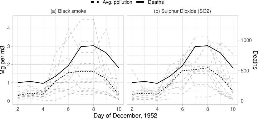
Figure 1: Pollution and mortality during the London smog of December 1952.

Historical measurements of pollution (black smoke and $\text{SO}_{2}$) from stations in London in December 1952. Each of the gray dashed lines represents the pollution measurements by a specific station. The dotted black line indicates the daily mean across all stations. The number of deaths in the Greater London area is overlaid with a solid black line. Pollution is digitised from Table I in [118] while deaths are digitised from Table VIII in [78].

Only levels of smoke and sulphur dioxide were measured at the time. However, as discussed in [118], it is likely that there were increases in tar, carbon monoxide (due to severe traffic congestion), carbon dioxide (due to a strong correlation with sulphur dioxide) and sulphuric acid (due to the oxidation of sulphuric dioxide). The nature of the smog also meant that it did not restrict itself to low-income areas, with the most affluent boroughs such as Kensington and Chelsea, as well as poorer boroughs such as Lambeth and Southwark being among the worst affected [118].

Although Londoners were used to smogs, the one in December 1952 was worse than any event Londoners had experienced before. Due to the dramatically reduced visibility, all public transport other than the London Underground was suspended, most flights to London were diverted, ambulance services stopped, and – with its penetration into indoor areas – concerts, theatres and cinema screenings were cancelled. Outdoor sporting events were also cancelled [17, see, e.g.,].

Despite this, Londoners got on with everyday life, potentially since the health consequences of extreme pollution were unknown. However, medical statistics that were published in the following weeks showed a substantial increase in mortality, with an estimated 4,000 deaths caused by the smog. Indeed, the right vertical axis of Figure 1 presents the daily number of deaths over the period of the smog, depicted as the solid black line. This shows around 300 daily deaths before the smog, increasing to $\sim$900 at its peak, after which it reduced; a similar inverse U-shaped pattern as the pollution data [78].

Subsequent calculations showed that 90% of the excess deaths were among those aged 45 and over [83]. There was also an increase in mortality among newborns and infants, as well as foetal loss [59, 13], but these capture a relatively small proportion of the total increase. We come back to this later. However, also in the months after the London smog, mortality exceeded normal levels. About half of these excess deaths were attributed to bronchitis or pneumonia, with other increases observed in respiratory tuberculosis, lung cancer, coronary disease, myocardial degeneration and other respiratory disease [78].

3.  Data

Our primary dataset is the UK Biobank, a prospective, population-based cohort that contains detailed information on the health and well-being of approximately 500,000 individuals living in the United Kingdom. Recruitment and collection of baseline information occurred between 2006 and 2010, when participants were 40–69 years old. The data include information on demographics, physical and mental health, health behaviours, cognition, and economic outcomes, obtained via questionnaires, interviews, and measurement taken by nurses. It has also been linked to hospital records, as well as the National Death Registry. Furthermore, samples of blood, urine and saliva have been collected, and all individuals have been genotyped. [38] give a detailed description of the sample.

We are interested in the long term economic and health consequences of short term variation in the early-life pollution environment. We focus on a set of outcomes, each informed by previous literature on the effects of pollution. First, we build on the literature that shows medium-to-long term effects of early life pollution exposure on economic outcomes [5, 12, see e.g.,], investigating the effects on educational attainment and fluid intelligence. Educational attainment is defined based on individuals’ qualifications and fluid intelligence is a score based on problem solving questions that require logic and reasoning ability, independent of acquired knowledge. Unfortunately, there is no systematic data collection on individuals’ labour market outcomes and hence we cannot explore this.

Next, we build on the literature showing pollution effects on individuals’ health [48, see e.g.,] and explore the effects on respiratory disease, cardiovascular disease and cancer. We observe whether individuals are diagnosed with these conditions using the linkage to hospital records. As these records go back to 1997 for England and 1999 for Wales, we do not observe any earlier hospitalisations and hence, to the extent that individuals were diagnosed before these years but did not receive any treatment in the 10–15 years since, we may underestimate disease occurrence. The contemporaneous effects of air pollution on respiratory and cardiovascular disease are well-known. Less is known, however, about the potential long term effects of early life exposure. Indeed, since air pollution disproportionally affects individuals with compromised lung function, and much of the burden in adulthood is believed to be due to poor development of the lungs (rather than its accelerated decline; see e.g. [75]), early life pollution is a natural exposure to consider in the development of respiratory disease. Similarly, long-term exposure to air pollution has been shown to prematurely age blood vessels and lead to increased build up of calcium in the coronary artery, restricting blood flow to the heart [71]. Both of these channels can in turn lead to cancer, for example via the build up of nanoparticles in the lungs affecting the replication of cells.

We create dummy variables to indicate whether the individual has been diagnosed with respiratory disease, cardiovascular disease, or cancer from the administrative hospitalisation data that have been merged into the UK Biobank. Furthermore, due to the links between respiratory disease and severe COVID-19 [11], and between short-term air pollution and COVID-19 [92, 10, 66], we additionally use a binary indicator for being hospitalised with, or having died from, COVID-19.

Using participants’ eastings and northings of birth, we assign each individual one of the 1472 Local Government Districts of birth across England and Wales. This spatial information, in combination with temporal information on individuals’ year-month of birth, allows us to identify individuals who were exposed to the smog at different time points during the intrauterine and early childhood period. We split our sample along the time dimension by considering whether the prenatal period precedes, overlaps, or follows the smog event on December 5-9th, 1952. This allows us to define three groups: (i) those exposed to the smog during childhood (i.e., those born before the smog), (ii) those exposed to the smog in utero, and (iii) those conceived after the smog event and therefore not exposed.

We split our sample along the spatial dimension by identifying the geographical areas in and around London that were exposed to high pollution during the smog. To do so, we overlay the reduced visibility and sulphur dioxide measurements from [118] onto a district-level shapefile, where we highlight some well-known landmarks for a better sense of scale. This is shown in Figure 2, where the solid black outlines indicate the areas with low and severe reductions in visibility and the dotted outline indicates the area with high sulphur dioxide measurements. We define “high exposure” districts as those that experienced severe reductions in visibility (i.e., overlap with the two inner solid boundaries in Figure 2) and/or experienced high sulphur dioxide measurements (i.e., overlap with the dotted boundary in Figure 2). Districts that only overlap with the outer solid boundary, indicating the mildest reduction in visibility, are classified as “low exposure”. In our main analysis, we do not distinguish between the high and low exposure districts but instead refer to them jointly as “treated” districts. We compare these treated districts to a set of “control” districts that are defined as other urban districts in England and Wales with a population density exceeding $400$ individuals per $\text{km}^{2}$. In our robustness checks, we explore the sensitivity of our results to control districts with different population densities, to excluding the “low exposure” districts, to assigning exposure based on individuals’ reported birth locations, as well as by defining control districts as other major cities in England and Wales.

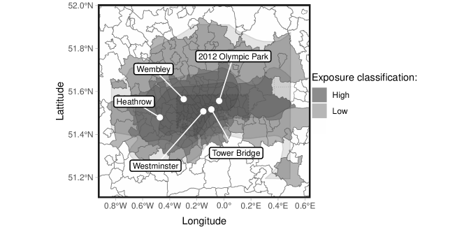
Figure 2: Visibility and pollution measurements during the London smog.

The geographic boundaries of the London smog based on the maps in [118]. The solid black outlines show the areas with reduced visibility. The inner boundaries experienced a more severe reduction in visibility. The dotted outline shows the area with high sulphur dioxide measurements. The map classifies the districts into ‘high exposure’ (dark gray), ‘low exposure’ (light gray), and ‘unexposed’ (white) districts. The white dots mark London landmarks (i.e., Heathrow, Wembley, Westminster, Tower Bridge, and the 2012 Olympic Park) to help show the scale of the map.

Our sample selection process is as follows: we only consider the subsample of 332,393 individuals born in either treated or control districts, and restrict the sample to those born from December 1950 to December 1956, resulting in 66,139 individuals. Furthermore, we follow the (genetics) literature and restrict our sample to those of white European ancestry, dropping 1,058 individuals. This leaves us with between 26,877–65,060 participants for the main analysis, depending on the outcome of interest.

Given the potential importance of the weather for exposure to smog as well as impacts of the weather on individuals’ health [60, see e.g.], we merge in two auxiliary datasets that give an interpolated grid of measurements on ambient temperature, sunshine, wind speed, and rainfall at the time of the smog. For temperature, rain and sunshine, these data are available from the MET Office [81], while, for wind, we use the ERA5 reanalysis data [63]. The datasets have an approximate grid resolution of 25km and we assign measurements to individuals by linking their location of birth, as measured in eastings and northings, to its nearest grid point. We merge in the weather data at individuals’ birth location for the period of the smog. For ambient temperature, we assign the minimum temperature measured during the smog, while for sunshine, wind speed and rainfall, we use the average. Because the weather measurements link to individuals’ eastings and northings of birth (rather than their birth districts), these measurements vary within districts and capture local atmospheric conditions experienced at individuals’ birth locations at the time of the smog. Most of the variation in weather conditions, however, comes from between-district variation, with the within-district variation being relatively small.

Table 1 presents the descriptive statistics on the full sample (column 1) as well as distinguishing between the treated (column 2) and control (column 3) samples. Panel A shows the statistics for individuals, while Panel B uses data from the Registrar General reports [108] and the 1951 UK Census to calculate district-level descriptives. Panel A shows that 44% of the sample is male and individuals, on average, have 13.3 years of education. Individuals’ fluid intelligence is only available for a smaller sample of individuals, which we standardise to have mean zero and unit variance on the full sample. 14.2% of the individuals have been hospitalised with cancer, while it is 19.2% for cardiovascular disease and 9.2% for respiratory disease. Finally, 0.7% of our sample has been either hospitalised or has died with COVID-19 as primary or secondary cause. For the districts, Panel B shows an average of 15 births and 13 deaths per 1,000 population, and an infant ($<1$ year) and neonatal ($<4$ weeks) mortality rate of 30 and 19 respectively per 1,000 live births. The main occupation share is from skilled occupations (53%). For most of the variables, treated districts perform slightly ‘better’ than control districts, with individuals in treated districts having higher education and fluid intelligence, as well as a lower probability of being hospitalised. Comparing the shares of workers in the five occupation classes of the 1951 census, control districts have a larger share of partly skilled workers, while treated districts have a higher share of workers in professional and intermediate occupations. The shares of skilled and unskilled workers are similar.

Table 1: Descriptive statistics for the main outcomes and variables.

	Estimation sample			Treated			Control
	Mean	SD	Obs.	Mean	SD	Obs.	Mean	SD	Obs.
Panel (a) – Individuals
Male	$0.443$	0.497	65,060	$0.447$	0.497	11,011	$0.443$	0.497	54,049
Educational attainment	$13.317$	2.274	64,681	$13.791$	2.242	10,953	$13.221$	2.268	53,728
Fluid intelligence	$-0.000$	1.000	26,877	$0.078$	1.003	5,666	$-0.021$	0.998	21,211
Cancer	$0.142$	0.349	64,926	$0.140$	0.347	10,991	$0.142$	0.349	53,935
Cardio-vascular disease	$0.192$	0.394	64,933	$0.167$	0.373	10,991	$0.197$	0.398	53,942
Respiratory disease	$0.092$	0.290	64,923	$0.080$	0.272	10,988	$0.095$	0.293	53,935
COVID-19	$0.007$	0.081	65,060	$0.005$	0.071	11,011	$0.007$	0.083	54,049
Panel (b) – Districts
Shares of occupations
– Professional	$0.036$	0.026	805	$0.053$	0.036	121	$0.034$	0.023	684
– Intermediate	$0.147$	0.058	805	$0.169$	0.059	121	$0.143$	0.057	684
– Skilled	$0.531$	0.055	805	$0.537$	0.056	121	$0.530$	0.055	684
– Partly skilled	$0.157$	0.067	805	$0.115$	0.033	121	$0.164$	0.069	684
– Unskilled	$0.129$	0.047	805	$0.126$	0.056	121	$0.129$	0.045	684
Birth rate	$0.015$	0.002	809	$0.015$	0.002	124	$0.015$	0.003	685
Death rate	$0.013$	0.003	809	$0.011$	0.002	124	$0.014$	0.003	685
Death rate, $<$ 1 year	$0.030$	0.014	809	$0.024$	0.008	124	$0.031$	0.015	685
Death rate, $<$ 4 weeks	$0.019$	0.013	809	$0.017$	0.007	124	$0.020$	0.014	685

• Panels: (a) descriptives calculated on individual-level data, (b) descriptives calculated at the district-level using data from the Registrar General reports and the 1951 census. The columns report sample means, sample standard deviations, and number of observations, in, respectively, the full sample, the treated districts and the control districts. Birth and death rates are measured per 1,000 births/population.

4.  Empirical strategy

To investigate the long term effects on human capital and health outcomes of early life pollution exposure, we exploit spatio-temporal variation in exposure to the London smog across birth dates and residential locations using a ‘reverse difference-in-difference’ approach. We observe the eastings and northings of individuals’ residential location at birth, with a 1km resolution. We distinguish between those born inside and outside the exposed London area (spatial variation) while also considering the timing of birth relative to the smog event (temporal variation). Our main specification is:

$$Y_{ijt} =\alpha_{j}+\gamma_{t}+\tau_{k}t+\beta_{IU}E^{IU}_{i}\times L_{j}+\beta_{CH}E^{CH}_{i}\times L_{j}+\theta_{IU}E^{IU}_{i}+\theta_{CH}E^{CH}_{i}+\delta\mathbf{X}_{i}+\epsilon_{ijt},$$ (1)

where $Y_{ijt}$ denotes the outcome of interest for individual $i$, born in district $j$ in year $t$. Thus, $\alpha_{j}$ denote district fixed effects, and $\gamma_{t}$ are year of birth fixed effects. We additionally include administrative-county-specific time (year-month) trends, denoted by $\tau_{k}t$. The vector $\mathbf{X}_{i}$ includes weather conditions during the smog, gender, and month-of-birth dummies to account for weather effects, gender differences, and seasonality in the outcome. Recall that the weather conditions are linked to individuals’ eastings and northings, meaning that we can identify their impacts also in a specification that includes district fixed effects. The indicators $E^{IU}_{i}$ and $E^{CH}_{i}$ are dummy variables that are equal to one for individuals who are in utero and in childhood (i.e., $<$age 2) respectively during the time of the smog, while $L_{j}$ is a binary variable that indicates whether the individual is born in an area of London that was exposed to the smog (i.e., in treated districts). Hence, our identification strategy compares individuals’ outcomes $Y_{ijt}$ for those exposed at different ages (i.e., in utero and in early childhood) to those conceived after the London smog in treated districts, relative to others born at the same time, but in control districts. The parameters of interest are therefore $\beta_{IU}$ and $\beta_{CH}$ which parameterise, respectively, the long-term effects of being exposed to the smog in utero and in early childhood, relative to non-exposed cohorts, accounting for any administrative county-specific trends in $Y_{ijt}$, time and district fixed effects. We use robust standard errors, clustered by district throughout.

Our specification implicitly assumes that individuals who were born in districts that were affected by the London smog would have had similar trends in their outcomes of interest in the absence of the smog compared to those born in districts that were not affected. We explore this common trend assumption empirically in Appendix C. Since those born prior to the smog may have been exposed in early childhood, we should find common trends among those conceived after the smog in treated and control districts. We find no evidence to suggest that those born in treated districts have differential trends in the outcomes of interest compared to those born control districts.

Because we use a ‘reverse’ difference-in-difference approach, comparing individuals conceived before/during the smog (i.e., affected in utero or in childhood) to those conceived afterwards, the validity of our approach also relies on the assumption that the outcomes of those conceived after the smog are the same as what would have been observed in the absence of the smog. This implicitly assumes away differential pollution avoidance behaviour post-smog in treated and control districts. Indeed, if individuals in both treated and control districts engaged in similar avoidance behaviour (e.g., closing windows in polluted areas), our difference-in-difference approach cancels these out and we would still obtain an unbiased estimate of the effect of exposure to the London smog. However, if those in treated districts engaged in more pollution avoidance behaviour compared to those in control districts, we may overestimate the impact of the London smog. In this case, our estimate captures (i) the actual effect of increased smog exposure as well as (ii) a larger decrease in exposure post-smog among those in treated districts compared to those in control districts, overestimating the difference.

Similarly, we assume that individuals’ residence choices did not change systematically after the smog. Although we cannot test this directly, we explore the validity of this assumption indirectly in two ways. First, we examine changes in the socio-economic composition of treated and control districts pre- and post-smog. In the absence of annual systematic data collection on each districts’ socio-economic composition, we use the 1951, 1961 and 1971 censuses and plot the average district-level share of high and low social class households (defined using individuals’ occupation) in each of the census years. The results, presented in Figure A.4 in Appendix A, shows that the average share of high and low social class households in treated and control districts remains relatively stable over time. We find a slight increase in the share of low social class households in treated districts between 1951 and 1961, but the change is negligible, both in absolute terms (0.013 percentage points) and in relative terms (relative to a standard deviation of 0.08).

In the absence of data on household moves or parental residential location choices, the second way in which we explore the validity of the assumption that the London smog did not affect individuals’ choice of residence is by exploiting the location of birth for a smaller set of sibling pairs (identified using the genetic kinship data). We specify a binary variable $move_{st}$ to equal one if sibling pair $s$ with (firstborn’s) year of birth $t$ reports different locations of birth. Within our sample of sibling pairs, some are both born before the smog, whilst for others, one sibling is born before and one after the smog. We restrict this sample to sibling pairs where the first sibling was born between 1946-1952 in the same districts as those used in our main analysis, and where the siblings are at most five years apart, yielding $n=3,079$ sibling pairs. We denote the group of sibling-pairs where the youngest sibling was born after the smog as $Post$ and run the following regression:

$$move_{st} =\eta_{0}+\eta_{1}Post_{t}+\eta_{2}Treated_{s}+\eta_{3}Treated_{s}\times Post_{t}+\eta_{4}age_{s}+u_{st},$$ (2)

where $Treated_{s}$ is a binary indicator that equals one if the older sibling is born in treated districts, and $age_{s}$ captures the age of the oldest sibling when at the birth of the younger sibling. We run this regression both with and without (the older child’s) district, year-of-birth and month-of-birth fixed effects, capturing whether – for cohorts where one sibling is born after the smog – they are more likely to move if the first child was born in treated compared to control areas. Note that $Treated_{s}$ drops out when we include district fixed effects. We report the estimates in Table A.2 in Appendix A. The parameter $\eta_{1}$ essentially captures a cohort effect, indicating whether sibling pairs with a younger sibling born after the smog are systematically different in terms of moving probabilities compared to those where both siblings were born before the smog. We find no such evidence. In the specification without fixed effects, the parameter $\eta_{2}$ however, shows that sibling pairs where the first sibling was born in a treated district are 25 percentage points more likely to move in between the births of two siblings compared to sibling pairs where the first sibling was born in a control district. We find no evidence though that this probability is different for sibling pairs where the youngest was born after the smog, as captured by the parameter on the interaction ($\eta_{3}$). The estimates, both with and without fixed effects, are small (2 and 4 percentage points, respectively) and statistically insignificant, suggesting that the London smog did not significantly increase the probability of moving for those with an older sibling born in treated districts.

Another important issue in the above specification is potential (foetal) selection. Indeed, there is evidence of increased mortality among newborns and infants [83], as well as foetal loss [59, 13]. Although these effects were relatively small as the smog mainly affected deaths among the elderly [83], they do affect our analysis and interpretation. More specifically, assuming that the smog increased mortality among relatively frail infants, leaving the stronger ones to survive, this may have led to an improvement in average cohort-level human capital and health outcomes for those exposed in the affected districts. This, in turn, suggests that our estimates may be underestimates of the effects of interest. We report our analyses on the impacts of the smog on the annual birth, death and infant mortality rate in more detail in Figure A.5 in Appendix A, where we find strong evidence of an increase in total annual deaths in 1952 and 1953, some evidence of a reduction in births in 1953 – potentially driven by foetal loss – but no significant effects on infant mortality.

Finally, the fact that the London smog only lasted five days additionally allows us to explore the gestational ages that are most sensitive to pollution exposure. This identification exploits the fact that the period of pollution exposure is substantially shorter than the length of gestation. To do this, we replace $E^{IU}_{i}$ in Equation 1 with three binary variables indicating the trimester in which the individual was exposed to the London smog.

5.  Results

5.1.  The London smog

We start by examining the long-term impact of pollution exposure on human capital outcomes. Columns (1) and (2) of Table 2 show the estimates from Equation 1 for years of education and fluid intelligence respectively. We find no strong differences in the outcomes among individuals exposed to the London smog prenatally or in early childhood in control districts compared to those conceived afterwards. However, within treated districts, we find a reduction in fluid intelligence for those exposed in utero as well as in childhood. The latter show the largest negative effects, with $0.16$ standard deviations lower fluid intelligence score compared to those born at the same time in control districts. Being exposed in utero reduces fluid intelligence by $0.11$ standard deviations. Looking at the estimates for years of education, we find that they are of a similar magnitude, but they are not significantly different from zero at conventional levels. Table A.3 in Appendix A presents the results where we distinguish between different qualifications, showing the effect of exposure to the smog on the probability of exiting the education system with a degree (column 1), upper secondary (column 2; i.e., A/AS levels, or professional/vocational training), lower secondary (column 3; i.e., CSEs, GCSEs, O-levels), and no qualifications (column 4). This shows that the negative estimates for pre- and post-natal pollution exposure are mostly driven by a reduction in the probability of obtaining a degree or upper secondary qualification, and – correspondingly – a higher probability of exiting the education system with lower secondary qualifications.

Table 2: Difference-in-Difference estimates comparing treated to control districts defined as urban England and Wales.

	Dependent variable:
	(1)	(2)
	Educational attainment	Fluid intelligence
Treated $\times$ In utero	$-0.100$	$-0.112^{**}$
	$(0.089)$	$(0.051)$
Treated $\times$ Childhood	$-0.135$	$-0.158^{**}$
	$(0.088)$	$(0.068)$
In utero	$-0.003$	$0.008$
	$(0.054)$	$(0.036)$
Childhood	$-0.014$	$-0.051$
	$(0.120)$	$(0.074)$
Observations	64,681	26,877
Mean dep. var.	13.317	0
$R^{2}$	0.08	0.067

• Columns: (1) educational attainment in years, (2) standardised fluid intelligence score. Includes fixed-effects for district, month of birth, and year of birth. Also controls for gender, weather variation, and year-month linear time trends by administrative county. Urban England and Wales are defined as districts that had a population density above 400 individuals per km² in 1951. Standard errors are clustered by district. (*): $p<0.1$, (**): $p<0.05$, (***): $p<0.01$.

We now turn to the long-term consequences of pollution on health outcomes. Table 3, Column (1) presents the estimates from Equation 1 for respiratory disease. This shows an increase in the prevalence of respiratory disease for those exposed to the smog prenatally. More specifically, those in utero during the smog and born in the exposed areas are two percentage points more likely to be diagnosed with respiratory disease compared to those conceived after the smog. Considering that the overall incidence of respiratory disease is 9% in the sample, this is a large effect, similar to a 22% increase. To explore which respiratory conditions drive this increase in hospitalisation risk, we estimate separate regressions for each of the ICD-10 sub-categories that make up our respiratory outcome and report the results in Table A.4 in Appendix A. These estimates show that our results are driven by hospitalisations relating to influenza and pneumonia (J09-J18), with no impacts on any of the other ICD-10 sub-categories. To explore this further, we report this as a separate outcome in Column (2) of Table 3 as well as throughout our further analyses. Next, we examine whether the negative effect on respiratory disease translates into COVID-related deaths or hospitalisations in Column (3). With coefficients that are tightly estimated around zero, we find no evidence of increased COVID-related morbidity or mortality, and similarly, in Column (4), we do not find increased prevalence of hospitalisations due to cancer. Finally, in Column (5), we see no statistically significant increase in risk of being hospitalised with cardiovascular disease, but we note that the estimates both for prenatal and childhood exposure are larger in (absolute) magnitude than the estimates seen for cancer and COVID-19, giving some suggestive evidence of a relationship between smog exposure and late-life cardiovascular disease.

Table 3: Difference-in-Difference estimates comparing treated to control districts defined as urban England and Wales.

	Dependent variable:
	(1)	(2)	(3)	(4)	(5)
	Respiratory, any	Influenza/ pneumonia	COVID-19	Cancer	Cardio- vascular
Treated $\times$ In utero	$0.020^{*}$	$0.012^{**}$	$0.000$	$-0.003$	$0.011$
	$(0.011)$	$(0.005)$	$(0.003)$	$(0.013)$	$(0.015)$
Treated $\times$ Childhood	$-0.007$	$0.009$	$-0.001$	$-0.001$	$0.007$
	$(0.012)$	$(0.006)$	$(0.003)$	$(0.014)$	$(0.019)$
In utero	$-0.005$	$-0.006$	$0.000$	$-0.005$	$-0.004$
	$(0.006)$	$(0.004)$	$(0.002)$	$(0.008)$	$(0.010)$
Childhood	$-0.008$	$-0.002$	$-0.001$	$-0.009$	$-0.015$
	$(0.014)$	$(0.007)$	$(0.004)$	$(0.016)$	$(0.023)$
Observations	64,923	64,917	65,060	64,926	64,933
Mean dep. var.	0.092	0.027	0.007	0.142	0.192
$R^{2}$	0.018	0.016	0.013	0.016	0.03

• Columns: (1) ever hospitalised due to respiratory disease, (2) ever hospitalised due to influenza/pneumonia, (3) hospitalisation or death due to COVID-19, (4) ever hospitalised due to cardio-vascular disease, (5) ever hospitalised due to cancer. Includes fixed-effects for district, month of birth, and year of birth. Also controls for gender, weather variation, and year-month linear time trends by administrative county. Urban England and Wales are defined as districts that had a population density above 400 individuals per km² in 1951. Standard errors are clustered by district. (*): $p<0.1$, (**): $p<0.05$, (***): $p<0.01$.

Next, we examine the impact of the timing of exposure relative to individuals’ gestational age. For brevity, we further only report the estimates for education, fluid intelligence, and respiratory conditions (including influenza/pneumonia), since further analysis did not show significant long-term effects on COVID-19, cancer and cardiovascular disease. Table 4 shows the estimates for Equation 1, where we replace the indicator for in utero exposure, $E_{i}^{IU}$, with three indicators for the relevant trimesters. For years of education, this suggests that second trimester exposure is the most important and reduces education by 0.2 years on average, with third trimester and childhood exposure also showing negative effects, though these are not significantly different from zero. For fluid intelligence, we find the largest effects for first trimester exposure, reducing slightly with gestational age. The intrauterine effect on respiratory conditions, shown in column (3), is mainly driven by exposure in the first and, to a lesser extent, the second trimester. However, for influenza/pneumonia in column (4), we find similar estimates across childhood and trimesters, suggesting that the effect does not depend on the timing of exposure.

Table 4: Trimester effects. Difference-in-Difference estimates comparing treated to control districts defined as urban England and Wales.

	Dependent variable:
	(1)	(2)	(3)	(4)
	Educational attainment	Fluid intelligence	Respiratory, any	Influenza/ pneumonia
Treated $\times$ In utero, 1. tri.	$0.064$	$-0.147^{**}$	$0.032^{*}$	$0.011$
	$(0.134)$	$(0.073)$	$(0.018)$	$(0.008)$
Treated $\times$ In utero, 2. tri.	$-0.220^{*}$	$-0.120^{*}$	$0.019$	$0.012$
	$(0.118)$	$(0.068)$	$(0.016)$	$(0.008)$
Treated $\times$ In utero, 3. tri.	$-0.144$	$-0.068$	$0.009$	$0.013^{*}$
	$(0.121)$	$(0.089)$	$(0.015)$	$(0.008)$
Treated $\times$ Childhood	$-0.143$	$-0.155^{**}$	$-0.008$	$0.009^{*}$
	$(0.088)$	$(0.069)$	$(0.012)$	$(0.006)$
In utero 1. tri.	$-0.007$	$-0.010$	$-0.004$	$-0.008$
	$(0.063)$	$(0.047)$	$(0.008)$	$(0.006)$
In utero 2. tri.	$-0.049$	$0.006$	$0.003$	$-0.004$
	$(0.061)$	$(0.040)$	$(0.009)$	$(0.005)$
In utero 3. tri.	$0.084$	$0.042$	$-0.023^{***}$	$-0.008$
	$(0.081)$	$(0.051)$	$(0.008)$	$(0.005)$
Childhood	$0.066$	$-0.009$	$-0.027^{*}$	$-0.003$
	$(0.134)$	$(0.080)$	$(0.015)$	$(0.008)$
Observations	64,681	26,877	64,923	64,917
Mean dep. var.	13.317	0	0.092	0.027
$R^{2}$	0.08	0.067	0.018	0.016

• Columns: (1) educational attainment in years, (2) standardised fluid intelligence score, (3) ever hospitalised due to respiratory disease, (4) ever hospitalised due to influenza/pneumonia. Includes fixed-effects for district, month of birth, and year of birth. Also controls for gender, weather variation, and year-month linear time trends by administrative county. Urban England and Wales are defined as districts that had a population density above 400 individuals per km² in 1951. Standard errors are clustered by district. (*): $p<0.1$, (**): $p<0.05$, (***): $p<0.01$.

5.2.  Treatment effect heterogeneity

We next explore potential heterogeneity of treatment effects. For this, we investigate three sources of variation: heterogeneity with respect to gender, socio-economic status and individuals’ genetic ‘predisposition’. We discuss each in turn.

5.2.1.  Heterogeneity by gender

First, we investigate whether the effect of exposure to the smog is similar for men and women. Table 5 presents the estimates for our main outcomes of years of education, fluid intelligence and respiratory disease, with Panel (a) and (b) presenting the estimates for women and men, respectively. This shows that the negative effect of smog exposure on years of education in the full sample is largely driven by women, with much smaller effect estimates for men. Having said that, however, we cannot reject the null that the two estimates are the same. For fluid intelligence and respiratory disease, including influenza/pneumonia, we do not see large differences between men and women, though the estimates are not always significantly different from zero due to the reduced sample sizes and with that, larger standard errors.

Table 5: Heterogeneity across sex. Difference-in-Difference estimates comparing treated to control districts defined as urban England and Wales.

	Dependent variable:
	(1)	(2)	(3)	(4)
	Educational attainment	Fluid intelligence	Respiratory, any	Influenza/ pneumonia
Panel (a) – Female
Treated $\times$ In utero	$-0.118$	$-0.074$	$0.020$	$0.014^{**}$
	$(0.128)$	$(0.072)$	$(0.013)$	$(0.007)$
Treated $\times$ Childhood	$-0.238^{*}$	$-0.152^{*}$	$-0.010$	$0.006$
	$(0.130)$	$(0.083)$	$(0.015)$	$(0.008)$
In utero	$0.077$	$-0.028$	$-0.004$	$-0.008$
	$(0.074)$	$(0.048)$	$(0.008)$	$(0.005)$
Childhood	$0.127$	$-0.064$	$-0.012$	$-0.002$
	$(0.149)$	$(0.114)$	$(0.018)$	$(0.010)$
Observations	$35,972$	$14,909$	$36,110$	$36,105$
Mean dep. var.	$13.273$	$0$	$0.084$	$0.024$
$R^{2}$	$0.089$	$0.084$	$0.028$	$0.027$
Panel (b) – Male
Treated $\times$ In utero	$-0.084$	$-0.162^{*}$	$0.022$	$0.013$
	$(0.113)$	$(0.085)$	$(0.017)$	$(0.010)$
Treated $\times$ Childhood	$-0.022$	$-0.184^{*}$	$-0.003$	$0.017^{*}$
	$(0.135)$	$(0.105)$	$(0.019)$	$(0.010)$
In utero	$-0.080$	$0.055$	$-0.007$	$-0.004$
	$(0.077)$	$(0.051)$	$(0.010)$	$(0.006)$
Childhood	$-0.159$	$-0.026$	$-0.004$	$-0.000$
	$(0.175)$	$(0.103)$	$(0.023)$	$(0.013)$
Observations	$28,645$	$11,830$	$28,748$	$28,747$
Mean dep. var.	$13.373$	$0$	$0.103$	$0.03$
$R^{2}$	$0.098$	$0.095$	$0.032$	$0.029$

• Columns: (1) educational attainment in years, (2) standardised fluid intelligence score, (3) ever experienced a (primary) respiratory hospitalisation, (4) same as (3) but looking only at influenza/pneumonia. Panels: (a) female subsample, (b) male subsample. Includes fixed-effects for district, month of birth, and year of birth. Also controls for gender, weather variation, and year-month linear time trends by administrative county. Urban England and Wales are defined as districts that had a population density above 400 individuals per km² in 1951. Standard errors are clustered by district. (*): $p<0.1$, (**): $p<0.05$, (***): $p<0.01$.

5.2.2.  Heterogeneity by social class

We next explore potential treatment effect heterogeneity with respect to social class. Although the UK Biobank does not include data on individuals’ (or parental) socio-economic position at birth, and because individuals’ socio-economic position in adulthood is endogenous to the smog exposure, we merge the 1951 UK Census to the UK Biobank, allowing us to characterise the local area of birth in terms of its socio-economic composition relative to other areas in England and Wales. As such, we create a measure of social class based on individuals’ occupation at the district level, capturing the share of its population in professional, managerial and technical occupations. We define districts to be of ‘high social class’ if they are above the median of this distribution; we define ‘low social class’ districts as those below the median.

We estimate the main specification for these ‘high class’ and ‘low class’ subsamples and report the results in Table 6. Overall, we find slightly larger adverse effects of smog exposure among the lower social classes, but with the reduced sample sizes, the standard errors are larger and the estimates are not always significantly different from zero. The larger estimates among the low social classes suggest that the impact is disproportionally felt among those born in districts characterised by a lower socio-economic status. Note that this is unlikely to be driven by differential exposure to pollution across districts with different socio-economic compositions, since both poor and affluent districts were similarly affected by the smog [118, 12].

Table 6: Heterogeneity across social class. Difference-in-Difference estimates comparing treated to control districts defined as urban England and Wales.

	Dependent variable:
	(1)	(2)	(3)	(4)
	Educational attainment	Fluid intelligence	Respiratory, any	Influenza/ pneumonia
Panel (a) – High class
Treated $\times$ In utero	$-0.038$	$-0.099$	$0.020$	$0.008$
	$(0.132)$	$(0.097)$	$(0.015)$	$(0.008)$
Treated $\times$ Childhood	$0.022$	$-0.122$	$-0.009$	$0.015^{*}$
	$(0.129)$	$(0.117)$	$(0.016)$	$(0.008)$
In utero	$-0.104$	$-0.126$	$0.005$	$0.002$
	$(0.128)$	$(0.084)$	$(0.014)$	$(0.009)$
Childhood	$0.023$	$-0.150$	$0.044$	$0.019$
	$(0.238)$	$(0.163)$	$(0.031)$	$(0.015)$
Observations	$14,470$	$6,637$	$14,488$	$14,486$
Mean dep. var.	$13.91$	$0$	$0.078$	$0.022$
$R^{2}$	$0.080$	$0.075$	$0.028$	$0.026$
Panel (b) – Low class
Treated $\times$ In utero	$-0.086$	$-0.038$	$0.028$	$0.014$
	$(0.140)$	$(0.083)$	$(0.021)$	$(0.010)$
Treated $\times$ Childhood	$-0.321^{**}$	$-0.188^{*}$	$-0.016$	$-0.002$
	$(0.145)$	$(0.111)$	$(0.023)$	$(0.010)$
In utero	$0.019$	$0.048$	$-0.009$	$-0.009^{*}$
	$(0.060)$	$(0.039)$	$(0.007)$	$(0.005)$
Childhood	$-0.007$	$0.002$	$-0.021$	$-0.008$
	$(0.140)$	$(0.082)$	$(0.016)$	$(0.008)$
Observations	$49,656$	$19,923$	$49,878$	$49,874$
Mean dep. var.	$13.143$	$0$	$0.097$	$0.028$
$R^{2}$	$0.058$	$0.061$	$0.016$	$0.015$

• Columns: (1) educational attainment in years, (2) standardised fluid intelligence score, (3) ever experienced a (primary) respiratory hospitalisation, (4) same as (3) but only looks at influenza/pneumonia. Panels: (a) subsample with individuals born in ‘high class’ districts. (b) subsample with individuals born in ‘low class’ districts. Includes fixed-effects for district, month of birth, and year of birth. Also controls for gender, weather variation, and year-month linear time trends by administrative county. Urban England and Wales are defined as districts that had a population density above 400 individuals per km² in 1951. Standard errors are clustered by district. (*): $p<0.1$, (**): $p<0.05$, (***): $p<0.01$.

For educational attainment in Column (1), we find negative estimates among the lower social classes, and significantly so for childhood exposure. The estimates for childhood exposure in high and low social class districts are marginally significantly different from each other (p=0.08). For fluid intelligence in Column (2), we find negative estimates of pre- and postnatal exposure in both panels, though with variation in magnitude and statistical significance. Similar to the findings for educational attainment, these results suggest larger cognitive impacts of pollution exposure in childhood for individuals born in districts characterised by lower social classes. Turning to respiratory disease and influenza/pneumonia in Columns (3) and (4), we again find slightly larger estimates for intrauterine exposure among low social class districts, but we cannot statistically distinguish between them.

5.2.3.  Genetic heterogeneity

Finally, to directly incorporate the genetic component into the analysis, we construct variables measuring individuals’ ‘genetic predisposition’ to the outcomes of interest. We do this by running our own tailor-made Genome-Wide Association Study (GWAS) for each of the main outcomes on UK Biobank unrelated participants born in the years outside our analysis sample (i.e., 1934–1949 and 1957–1970), as well as those born in districts that are not defined as either treated or control during the study years 1950-1956. We use the summary statistics from this GWAS to construct so-called polygenic scores (also known as polygenic indices) for those in the (independent) analysis sample covering the birth cohorts 1950–1956. We do the latter using LDpred2, a Bayesian genetic risk prediction method [114, 97]. All polygenic scores are standardised to have mean zero and unit variance in the analysis sample.

Polygenic scores can be interpreted as the best linear genetic predictor of the outcome of interest [82]. However, this does not mean that it is an immutable, biological relationship. Indeed, in addition to any potential biological effect, the association may capture gene-environment correlation (also referred to as $rGE$), either via genetic variation invoking certain environmental responses (so-called evocative $rGE$), or via individuals selecting into certain environments based on their genetic variation (active $rGE$). Furthermore it captures ‘genetic nurture’ effects: the fact that parental genetic variation can shape the environment that the child experiences, which in turn can affect their outcome (an example of passive $rGE$; see also e.g., [74]). In short, this implies that the predictive power of the polygenic score, as shown in Table D.2 in Appendix D, may capture both genetic as well as environmental components. Nevertheless, it allows us to investigate previously unobserved heterogeneity in the effect estimates and with that, quantify the extent to which one’s genetic variation may protect or exacerbate the effects of early life adverse circumstances.

Table 7 presents the main difference-in-difference estimates distinguishing between individuals with a high versus low genetic ‘predisposition’ to the outcome, defined as having a polygenic score above or below the median, shown in Panel (a) and (b) respectively. Note that the polygenic score is specific to the outcome of interest to avoid any potential data mining. For example, the polygenic score in Columns (1) and (2) of Table 7 is the best linear genetic predictor for education and fluid intelligence, respectively. This shows that the zero effect of the smog on educational attainment conceals substantial genetic heterogeneity. More precisely, the negative effect is substantially larger for those with a high polygenic score for education, for both prenatal and childhood exposure (though we only reject the null that the estimates are the same for prenatal exposure; $p=0.06$), with the estimates being close to zero for those with a polygenic score below the median.

Table 7: Heterogeneity across genetics. Difference-in-Difference estimates comparing treated to control districts defined as urban England and Wales.

	Dependent variable:
	(1)	(2)	(3)	(4)
	Educational attainment	Fluid intelligence	Respiratory, any	Influenza/ pneumonia
Panel (a) – High polygenic score
Treated $\times$ In utero	$-0.249^{**}$	$-0.091$	$0.019$	$0.018^{**}$
	$(0.107)$	$(0.073)$	$(0.017)$	$(0.008)$
Treated $\times$ Childhood	$-0.197^{*}$	$-0.154$	$-0.015$	$0.017^{*}$
	$(0.118)$	$(0.095)$	$(0.019)$	$(0.010)$
In utero	$-0.010$	$0.020$	$-0.016^{*}$	$-0.008$
	$(0.075)$	$(0.050)$	$(0.010)$	$(0.006)$
Childhood	$-0.168$	$-0.052$	$-0.007$	$-0.004$
	$(0.164)$	$(0.096)$	$(0.020)$	$(0.011)$
Observations	$32,376$	$13,571$	$32,423$	$32,420$
Mean dep. var.	$13.911$	$0$	$0.104$	$0.031$
$R^{2}$	$0.083$	$0.087$	$0.030$	$0.027$
Panel (b) – Low polygenic score
Treated $\times$ In utero	$0.096$	$-0.086$	$0.022$	$0.007$
	$(0.152)$	$(0.084)$	$(0.014)$	$(0.008)$
Treated $\times$ Childhood	$-0.010$	$-0.113$	$0.007$	$0.005$
	$(0.161)$	$(0.104)$	$(0.016)$	$(0.008)$
In utero	$-0.016$	$-0.028$	$0.007$	$-0.005$
	$(0.068)$	$(0.047)$	$(0.008)$	$(0.005)$
Childhood	$0.111$	$-0.038$	$-0.006$	$0.000$
	$(0.152)$	$(0.113)$	$(0.018)$	$(0.009)$
Observations	$32,233$	$13,162$	$32,442$	$32,439$
Mean dep. var.	$12.721$	$0$	$0.081$	$0.023$
$R^{2}$	$0.075$	$0.084$	$0.029$	$0.028$

• Columns: (1) educational attainment in years, (2) standardised fluid intelligence score, (3) ever experienced a (primary) respiratory hospitalisation, (4) same as (3) but only looks at influenza/pneumonia. Panels: (a) subsample with above-median polygenic score. (b) subsample with below-median polygenic score. Includes fixed-effects for district, month of birth, and year of birth. Also controls for year-month linear time trends by administrative county. Urban England and Wales are defined as districts that had a population density above 400 individuals per km² in 1951. Standard errors are clustered by district. (*): $p<0.1$, (**): $p<0.05$, (***): $p<0.01$.

To explore what may be driving the negative effect on educational attainment for those with a high polygenic score, Table A.10 in Appendix A examines the effects of pollution exposure on the probability of reaching different levels of qualifications. This shows that the negative effect of pre- and post-natal pollution exposure for those with a high polygenic score is driven by a reduction in the probability of obtaining an degree or upper secondary qualification and – correspondingly – a higher probability of lower secondary or no qualifications. This suggests that pollution exposure reduces one’s human capital potential, in particular among those with a high genetic potential.

There is little difference between the estimates for individuals with high and low polygenic scores for fluid intelligence, with both showing a negative effect of smog exposure, though with the smaller sample sizes, they are not significantly different from zero. Furthermore, while the effects of prenatal smog exposure on respiratory disease are similar across subgroups, we find that for influenza/pneumonia the effects of both prenatal and childhood exposure are somewhat larger for those with a high polygenic score, suggesting that the respiratory health of individuals who are genetically ‘predisposed’ is more vulnerable to severe pollution events, though the differences between those with high and low polygenic scores are not significant at conventional levels.

6.  Robustness analysis

We next present a range of sensitivity analyses to explore the robustness of our main findings. First, we investigate the sensitivity of our estimates to the definition of treatment and control groups. Second, we explore whether our estimates are robust to different definitions of the reference group (i.e., those conceived after the smog). Third, we examine whether the exposure effects differ for exposure in infancy versus early childhood. In all robustness checks, we run our analyses only on the three main outcomes: educational attainment, fluid intelligence and respiratory disease.

6.1.  Definition of treated and control districts

We start by exploring the sensitivity of our estimates to (1) alternative definitions of treated districts, and (2) alternative definitions of control districts. First, we consider different definitions of the exposed districts. The results are reported in Table 8. In Panel (a), we start by dropping the districts classified as low exposure (defined in Section 3). Assuming these districts were less exposed compared to Central London, excluding them may increase our effect estimates. Panel (a) indeed shows that dropping low exposure districts results in estimates that are similar or slightly larger relative to those in the main analysis.

To reduce measurement error in the exposure classifications, Panel (b) exploits the actual residential locations at birth of individuals (at a 1 km² resolution) and assigns exposure based on the individual’s eastings and northings of birth relative to the pollution boundaries (as opposed to assigning treatment based on whether individuals’ district of birth is in the smog-affected area, as in the main specification). Table 8 shows that excluding individuals born outside the high exposure boundaries, but in districts that are (at least partially) exposed does not affect our estimates.

Table 8: Definition of exposure. Difference-in-Difference estimates comparing treated to control districts defined as urban England and Wales.

	Sample:
	(1)	(2)	(3)	(4)
	Educational attainment	Fluid intelligence	Respiratory, any	Influenza/ pneumonia
Panel (a) – Districts, low exposure dropped
Treated $\times$ In utero	$-0.121$	$-0.105^{**}$	$0.018$	$0.013^{**}$
	$(0.095)$	$(0.052)$	$(0.012)$	$(0.006)$
Treated $\times$ Childhood	$-0.147$	$-0.185^{***}$	$-0.015$	$0.007$
	$(0.090)$	$(0.068)$	$(0.013)$	$(0.006)$
In utero	$-0.001$	$0.012$	$-0.005$	$-0.006$
	$(0.054)$	$(0.036)$	$(0.006)$	$(0.004)$
Childhood	$-0.023$	$-0.033$	$-0.007$	$-0.000$
	$(0.121)$	$(0.074)$	$(0.014)$	$(0.007)$
Observations	$63,394$	$26,294$	$63,633$	$63,627$
Mean dep. var.	$13.301$	$0$	$0.093$	$0.027$
$R^{2}$	$0.077$	$0.066$	$0.018$	$0.016$
Panel (b) – Birth location
Treated $\times$ In utero	$-0.099$	$-0.100^{**}$	$0.020^{*}$	$0.011^{*}$
	$(0.091)$	$(0.051)$	$(0.011)$	$(0.006)$
Treated $\times$ Childhood	$-0.130$	$-0.136^{**}$	$-0.005$	$0.007$
	$(0.089)$	$(0.068)$	$(0.013)$	$(0.006)$
In utero	$-0.004$	$0.005$	$-0.005$	$-0.006$
	$(0.053)$	$(0.035)$	$(0.006)$	$(0.004)$
Childhood	$-0.016$	$-0.057$	$-0.008$	$-0.001$
	$(0.120)$	$(0.074)$	$(0.014)$	$(0.007)$
Observations	$64,681$	$26,877$	$64,923$	$64,917$
Mean dep. var.	$13.317$	$0$	$0.092$	$0.027$
$R^{2}$	$0.080$	$0.067$	$0.018$	$0.016$

• Columns: (1) educational attainment in years, (2) standardised fluid intelligence score, (3) ever hospitalised due to respiratory disease, (4) ever hospitalised due to influenza/pneumonia. Panels: (a) exposed districts defined as districts overlapping with any pollution boundary but districts with low exposure have been dropped, (b) exposed individuals defined as individuals with birth location inside any pollution boundary. The ‘control’ cities are: Bristol, Cardiff, Leicester, Liverpool, Manchester, Newcastle, Nottingham, Sheffield, and Birmingham (defined according to 1951 districts). Includes fixed-effects for district, month of birth, and year of birth. Also controls for gender, weather variation and linear time trends. Standard errors are clustered by district. (*): $p<0.1$, (**): $p<0.05$, (***): $p<0.01$.

Second, our main analysis defines control districts as those with a population density of at least 400 individuals per km². We here investigate the sensitivity of our results to this definition. Table 9 shows the estimates from Equation 1 for the main outcomes under different choices of the population density threshold used to define the control districts. From Panel (a) to (c) the control districts become more densely populated. For educational attainment in Column (1), we find insignificant negative estimates for exposure to the smog across the three panels. When using more densely populated control districts, the estimates for prenatal exposure move closer to zero relative to those in the main analysis, while those for postnatal exposure increase in (absolute) magnitude, and the standard errors become larger due to the reduction in sample size. The estimates for fluid intelligence in Column (2) increase in (absolute) magnitude as the control districts become more densely populated, particularly for childhood exposure. This suggests that the estimates vary somewhat depending on the definition of the control district. However, they are always negative, large, and significantly different from zero. In Columns (3) and (4), the effect of prenatal exposure to the smog on the likelihood of being diagnosed with respiratory disease is relatively robust to the use of more densely populated control districts.

Table 9: Sensitivity of main difference-in-difference estimates with respect to the urban density cutoff (population per km²).

	Dependent variable:
	(1)	(2)	(3)	(4)
	Educational attainment	Fluid intelligence	Respiratory, any	Influenza/ pneumonia
Panel (a) – 2,000 population per km2
Treated $\times$ In utero	$0.003$	$-0.154^{***}$	$0.021$	$0.015^{**}$
	$(0.103)$	$(0.055)$	$(0.013)$	$(0.006)$
Treated $\times$ Childhood	$-0.104$	$-0.221^{***}$	$-0.017$	$0.009$
	$(0.108)$	$(0.072)$	$(0.017)$	$(0.008)$
In utero	$-0.059$	$0.042$	$-0.009$	$-0.010^{**}$
	$(0.063)$	$(0.039)$	$(0.007)$	$(0.005)$
Childhood	$-0.069$	$-0.022$	$-0.009$	$-0.001$
	$(0.150)$	$(0.086)$	$(0.017)$	$(0.008)$
Observations	$46,908$	$20,210$	$47,104$	$47,099$
Mean dep. var.	$13.246$	$0$	$0.096$	$0.028$
$R^{2}$	$0.068$	$0.054$	$0.012$	$0.011$
Panel (b) – 3,000 population per km2
Treated $\times$ In utero	$-0.051$	$-0.203^{***}$	$0.027^{*}$	$0.018^{***}$
	$(0.111)$	$(0.058)$	$(0.015)$	$(0.007)$
Treated $\times$ Childhood	$-0.171$	$-0.302^{***}$	$-0.010$	$0.010$
	$(0.116)$	$(0.073)$	$(0.020)$	$(0.008)$
In utero	$-0.070$	$0.059$	$-0.010$	$-0.012^{**}$
	$(0.070)$	$(0.044)$	$(0.008)$	$(0.005)$
Childhood	$-0.044$	$-0.022$	$-0.016$	$-0.004$
	$(0.170)$	$(0.097)$	$(0.019)$	$(0.009)$
Observations	$38,057$	$16,650$	$38,228$	$38,224$
Mean dep. var.	$13.186$	$0$	$0.097$	$0.029$
$R^{2}$	$0.061$	$0.052$	$0.011$	$0.008$
Panel (c) – 4,000 population per km2
Treated $\times$ In utero	$-0.042$	$-0.165^{**}$	$0.021$	$0.014^{*}$
	$(0.129)$	$(0.066)$	$(0.018)$	$(0.008)$
Treated $\times$ Childhood	$-0.212$	$-0.360^{***}$	$-0.017$	$0.002$
	$(0.133)$	$(0.082)$	$(0.022)$	$(0.009)$
In utero	$-0.129$	$0.076$	$0.000$	$-0.006$
	$(0.088)$	$(0.054)$	$(0.008)$	$(0.006)$
Childhood	$-0.056$	$0.103$	$-0.007$	$0.009$
	$(0.181)$	$(0.110)$	$(0.026)$	$(0.011)$
Observations	$23,108$	$10,799$	$23,207$	$23,203$
Mean dep. var.	$13.218$	$0$	$0.098$	$0.029$
$R^{2}$	$0.057$	$0.049$	$0.012$	$0.008$

• Columns: (1) educational attainment in years, (2) standardised fluid intelligence score, (3) ever hospitalised due to respiratory disease, (4) ever hospitalised due to influenza/pneumonia. Panels show the estimates for different choices of the urban density cut off as measured in 1951. Includes fixed-effects for district, month of birth, and year of birth. Also controls for gender, weather variation, and year-month linear time trends by administrative county. Standard errors are clustered by district. (*): $p<0.1$, (**): $p<0.05$, (***): $p<0.01$.

Finally, instead of using population density to define the control districts, we use the main major cities in England and Wales: Birmingham, Bristol, Cardiff, Leicester, Liverpool, Manchester, Newcastle, Nottingham and Sheffield. Indeed, one interpretation of our results is that the treated not only have a pollution shock, but also face an accumulation of pollution throughout their childhood, which may affect their later-life health. By using specific major cities only in the control group, we ensure that both the treated and control groups experience heightened pollution throughout their early lives. Table 10 shows that this reduces the sample size substantially and with that, increases the standard errors. Despite that, the magnitude of the estimates are very similar to those reported above. This therefore suggests that our findings are not very sensitive to the definition of treatment and control districts.

Table 10: Difference-in-Difference estimates comparing treated to control cities.

	Dependent variable:
	(1)	(2)	(3)	(4)
	Educational attainment	Fluid intelligence	Respiratory, any	Influenza/ pneumonia
Treated $\times$ In utero	$-0.099$	$-0.177^{***}$	$0.020^{*}$	$0.016^{***}$
	$(0.105)$	$(0.050)$	$(0.012)$	$(0.006)$
Treated $\times$ Childhood	$-0.133$	$-0.269^{***}$	$0.000$	$0.016^{**}$
	$(0.099)$	$(0.077)$	$(0.017)$	$(0.008)$
In utero	$-0.040$	$0.071$	$-0.007$	$-0.012^{*}$
	$(0.083)$	$(0.053)$	$(0.008)$	$(0.006)$
Childhood	$-0.076$	$0.005$	$-0.016$	$-0.009$
	$(0.212)$	$(0.130)$	$(0.021)$	$(0.011)$
Observations	27,279	12,509	27,386	27,384
Mean dep. var.	13.276	0	0.093	0.027
$R^{2}$	0.072	0.042	0.012	0.009

• Columns: (1) educational attainment in years, (2) standardised fluid intelligence score, (3) ever hospitalised due to respiratory disease, (4) ever hospitalised due to influenza/pneumonia. The ‘control’ cities are: Bristol, Cardiff, Leicester, Liverpool, Manchester, Newcastle, Nottingham, Sheffield, and Birmingham (defined according to 1951 districts). Includes fixed-effects for district, month of birth, and year of birth. Also controls for gender, weather variation and linear time trends. Standard errors are clustered by district. (*): $p<0.1$, (**): $p<0.05$, (***): $p<0.01$.

6.2.  Definition of the reference group

Our main analysis compares those exposed to the smog in utero or in early childhood to those conceived after the smog. The latter (reference, or unexposed) group includes those born between September 1953 and December 1956. We next explore the sensitivity of this definition by restricting the year-months of birth of those in the reference group to be nearer the date of the smog. Panels (a) and (b) of Table 11 show the estimates of Equation 1 under two different choices of the end date used to define those who are not exposed to the smog: the end of 1954 and the end of 1955. Table 11 shows that our results are relatively stable across these alternative definitions of the reference (unexposed) group. For educational attainment in Column (1), when we restrict the reference group to be closer to the smog event, as shown in Panel (a) and (b), the effect of childhood exposure to the smog increases in absolute terms, but with a smaller sample size, the standard errors are larger and the confidence intervals always overlap with zero. The estimates for prenatal exposure remains around -0.1 across the two panels, but it is insignificantly different from zero throughout.

For fluid intelligence in Column (2), the estimates for prenatal and childhood exposure to the smog are negative, and very similar across the panels. The estimate for the effect of childhood exposure on the probability of being diagnosed with respiratory disease (Column (3)) increases in (absolute) magnitude and the effect of prenatal exposure reduces when we restrict the reference group. Finally, the intrauterine effect on the risk of hospitalisation with influenza/pneumonia is similar across panels (Column (4)), whilst there is a slight reduction in the estimates for childhood exposure as the reference group is further restricted.

Table 11: Sensitivity of main difference-in-difference estimates with respect to the after cutoff.

	Dependent variable:
	(1)	(2)	(3)	(4)
	Educational attainment	Fluid intelligence	Respiratory, any	Influenza/ pneumonia
Panel (a) – Controls from September 1953 to December 1954
Treated $\times$ In utero	$-0.103$	$-0.110^{**}$	$0.011$	$0.010^{*}$
	$(0.098)$	$(0.050)$	$(0.012)$	$(0.006)$
Treated $\times$ Childhood	$-0.181$	$-0.178^{**}$	$-0.031^{**}$	$0.002$
	$(0.119)$	$(0.082)$	$(0.016)$	$(0.008)$
In utero	$-0.003$	$0.040$	$0.001$	$-0.004$
	$(0.040)$	$(0.028)$	$(0.005)$	$(0.003)$
Childhood	$-0.027$	$0.047$	$0.009$	$-0.004$
	$(0.063)$	$(0.048)$	$(0.007)$	$(0.005)$
Observations	$45,232$	$18,770$	$45,395$	$45,390$
Mean dep. var.	$13.292$	$0$	$0.095$	$0.028$
$R^{2}$	$0.084$	$0.074$	$0.023$	$0.022$
Panel (b) – Controls from September 1953 to December 1955
Treated $\times$ In utero	$-0.096$	$-0.094^{**}$	$0.018$	$0.011^{*}$
	$(0.094)$	$(0.047)$	$(0.011)$	$(0.006)$
Treated $\times$ Childhood	$-0.127$	$-0.098$	$-0.014$	$0.005$
	$(0.106)$	$(0.068)$	$(0.014)$	$(0.007)$
In utero	$0.001$	$0.026$	$-0.000$	$-0.004$
	$(0.041)$	$(0.025)$	$(0.004)$	$(0.003)$
Childhood	$-0.010$	$-0.001$	$0.007$	$-0.003$
	$(0.053)$	$(0.036)$	$(0.007)$	$(0.004)$
Observations	$55,196$	$22,946$	$55,402$	$55,396$
Mean dep. var.	$13.308$	$0$	$0.093$	$0.028$
$R^{2}$	$0.081$	$0.072$	$0.020$	$0.018$

• Columns: (1) educational attainment in years, (2) standardised fluid intelligence score, (3) ever hospitalised due to respiratory disease, (4) ever hospitalised due to influenza/pneumonia. Panels show estimates under different choices of cutoff for defining the control cohorts born after the smog. Includes fixed-effects for district, month of birth, and year of birth. Also controls for gender, weather variation, and year-month linear time trends by administrative county. Urban England and Wales are defined as districts that had a population density above 400 individuals per km² in 1951. Standard errors are clustered by district. (*): $p<0.1$, (**): $p<0.05$, (***): $p<0.01$.

6.3.  Childhood exposure

We next explore whether the childhood exposure effect differs for exposure in infancy (age 0) or later (age 1). Table 12 presents the estimates that distinguish between the two ages in early childhood, showing that the effect on fluid intelligence is driven mainly by exposure in infancy. We also find larger effects on years of education for exposure in infancy. Although the effect of exposure at age 1 remains negative on education and intelligence, it is insignificantly different from zero for both outcomes.

Table 12: Childhood effects at age 0 and 1. Difference-in-Difference estimates comparing treated to control districts defined as urban England and Wales.

	Dependent variable:
	(1)	(2)	(3)	(4)
	Educational attainment	Fluid intelligence	Respiratory, any	Influenza/ pneumonia
Treated $\times$ In utero	$-0.093$	$-0.094^{*}$	$0.022^{**}$	$0.012^{**}$
	$(0.090)$	$(0.051)$	$(0.011)$	$(0.005)$
Treated $\times$ Childhood, age 0	$-0.142$	$-0.172^{**}$	$-0.010$	$0.009$
	$(0.088)$	$(0.067)$	$(0.012)$	$(0.006)$
Treated $\times$ Childhood, age 1	$-0.107$	$-0.089$	$0.005$	$0.010$
	$(0.114)$	$(0.082)$	$(0.015)$	$(0.008)$
In utero	$-0.012$	$0.005$	$-0.005$	$-0.006$
	$(0.055)$	$(0.036)$	$(0.006)$	$(0.004)$
Childhood, age 0	$-0.050$	$-0.043$	$-0.005$	$-0.001$
	$(0.126)$	$(0.079)$	$(0.015)$	$(0.007)$
Childhood, age 1	$-0.181$	$-0.045$	$0.001$	$-0.002$
	$(0.181)$	$(0.122)$	$(0.022)$	$(0.011)$
Observations	64,681	26,877	64,923	64,917
Mean dep. var.	13.317	0	0.092	0.027
$R^{2}$	0.08	0.067	0.018	0.016

• Columns: (1) educational attainment in years, (2) standardised fluid intelligence score, (3) ever experienced a (primary) respiratory hospitalisation, (4) same as (3) but only looks at influenza/pneumonia. Includes fixed-effects for district, month of birth, and year of birth. Also controls for gender, weather variation, and year-month linear time trends by administrative county. Urban England and Wales are defined as districts that had a population density above 400 individuals per km² in 1951. Standard errors are clustered by district. (*): $p<0.1$, (**): $p<0.05$, (***): $p<0.01$.

7.  Conclusions

There is a substantial literature documenting the contemporaneous effects of exposure to pollution on individuals’ human capital and health outcomes. Much less is known, however, about the potential longer-term effects of early-life pollution exposure, despite the fact that the intrauterine and early childhood environment are crucial for shaping individuals’ outcomes in older age. Indeed, most of the literature that investigates the effects of early-life pollution focuses on short-term effects, such as outcomes at birth, finding largely negative impacts. A lack of historical pollution data with good coverage of geographical locations means it is often not possible to use actual pollution measurements and relate those to later-life outcomes. To shed light on the longer-term effects, research instead has to rely on reduced form analysis and natural experiments. That is exactly what we do in this paper, estimating the very long-term effects of being exposed to a severe pollution event on a range of outcomes measured at age $\sim$60.

We present new evidence of the very long-term effects of an early-life pollution shock. The London smog affected Londoners between 5–9 December 1952, when a thermal inversion trapped pollution over London, which – due to weather conditions at the time – was not dispersed. We focus on the long-term human capital and health effects of exposure to the smog. We compare individuals exposed to the smog in London in either the intrauterine or infancy period to those born in other urban areas, as well as to those conceived after the smog. Our difference-in-difference analysis shows that those exposed to the smog have lower fluid intelligence scores, with some suggestive evidence that they also have fewer years of education. We find that exposure in infancy has slightly larger effects compared to exposure in utero. Investigating the long-term health effects, we find a large increase in the probability of being diagnosed with respiratory disease due to intrauterine exposure, which is driven by hospitalisations for influenza/pneumonia, with no impacts on cardiovascular disease and cancer diagnoses.

We next study potential differential effects of in utero exposure, distinguishing between exposure in the first, second, and third trimester. We find some evidence for differential gestational effects for fluid intelligence, with larger effects for exposure at early gestational ages. Similarly, we see that the increase in respiratory conditions is larger for first trimester exposure, but there is no evidence of trimester-specific effects for influenza/pneumonia.

We then model the heterogeneity of our effect estimates with respect to three sources of (predetermined) variation: gender, socio-economic status at birth, and individuals’ genetic predisposition. Although we often cannot reject the null that the estimates are the same across subgroups, our findings are suggestive of larger negative effects of pollution on schooling for women, larger impacts on human capital and respiratory health for those in low social class environments, as well as larger impacts on education and respiratory health among those genetically more susceptible to the outcome of interest.

Our estimates are quantitatively and qualitatively important, but there are four key points regarding their interpretation. First, they estimate the effects of exposure to a severe pollution event. Indeed, London nowadays experiences pollution levels that are still high, but nowhere near those observed in 1952. Hence, our results cannot be extrapolated to smog events occurring in London or most other cities in Europe nowadays. Despite that, they do compare to smog events that are happening each year in industrialising economies such as India and China. Hence, our findings are relevant to those settings, suggesting that such extreme pollution events do not only affect contemporaneous outcomes, but also have longer term adverse effects.

Second, our analysis compares pollution during the smog to ‘standard’ pollution levels in control districts as well as in the years immediately after the smog. Although these levels of pollution are indeed lower than those in inner London, they are not comparable to current levels of pollution. Hence, our estimates capture the effect of being exposed to a large pollution shock, relative to already high levels throughout early childhood. Again, the results can therefore better be extrapolated to industrialising economies with higher pollution levels in general, as well as larger pollution shocks.

Third, although we argue that the main cause of the reduction in human capital and health is the exposure to the smog, other potential channels are worth mentioning. For example, if the smog caused an increase in the probability of the mother losing one of her parents, this may have also affected her children through the longer-term effects of exposure to prenatal stress [94, see e.g.,].

Fourth, there is at least one reason to believe that our estimates are an upper bound of the ‘true’ effect of the smog, but also three reasons to believe they are a lower bound. If the smog differentially induced individuals to engage in pollution avoidance behaviour, their subsequent reduced exposure to pollution may lead us to over-estimate the effect of the smog. Although we cannot address this directly, the fact that we cannot reject the common trend assumption post-smog, that we find no differential trends in the socio-economic composition of treated and control districts, and no evidence of a differential probability of moving for sibling pairs across treated and control districts puts some confidence in our estimates.

Having said that, there are three reasons to believe we underestimate the long-term effects of the smog. First, the evidence suggests that the smog led to a small increase in infant mortality and foetal loss, and potentially a reduction in access to pre- and post-natal care. Assuming that those who were affected by this were more vulnerable and those who survived were stronger, this suggests that our estimates are likely to be a lower bound. Second, and relatedly, since individuals in the UK Biobank were invited to participate in 2006-2010, we implicitly condition on survival until this time. In the presence of frailty selection, where fragile individuals are more likely to die prior to assessment leaving stronger survivors in the sample, our estimates are likely to be attenuated. The third reason why our estimates are likely to be downward biased is due to measurement error. For one, since we do not observe gestational age, we assume all individuals were in utero for nine months prior to their year-month of birth, and we assume individuals were born on the first of the month. In reality, some individuals would have had a shorter gestational period, potentially misclassifying them as being exposed to the smog. Two, we are reliant on publications from the 1950s, showing the extent of the smog as well as its variability across London. We therefore define individuals as either exposed or unexposed, but in reality, pollution would have shown more regional variability that we are unable to capture in our analyses. Three, related to this, we observe individuals’ location of birth (eastings and northings) with a 1km resolution. Given that pollution changes across space, individuals who are born on the boundary of our exposed and unexposed districts may be misclassified, leading to additional measurement error.

As with any research, our analysis comes with its limitations. First, we cannot identify which pollutants matter more for individuals’ human capital and health outcomes. Indeed, the literature suggests that multiple pollutants increased during the smog, and we cannot determine whether one or more of these are driving the deterioration in later-life outcomes. Second, the UK Biobank is a large database of those aged 45–69 in the United Kingdom, but it is not representative, with its participants being healthier and wealthier than the UK population [55]. This has implications for our research and the interpretation of our findings. To the extent that air pollution disproportionately affects groups of lower socio-economic status, our results may not accurately reflect the impacts of pollution for these groups, potentially underestimating the overall impacts of pollution exposure. Having said that, the data is unique in combining information from questionnaires, objective measurements, genetic information, and administrative data on a very large sample of UK residents, with information on year-month and location of birth, allowing us to identify which participants were likely to be exposed and which were not. With that, our paper highlights the very long-run pollution effects, identifying reductions in individuals’ human capital and health outcomes up to $\sim$60 years after the actual exposure.

Finally, our findings have clear policy implications. They suggest that reducing pollution has large, long-term benefits for the population. From the population perspective, given the ease and low cost of pollution forecasting, the benefits of avoiding pollution are substantial. From a policy maker perspective, this should encourage the implementation of incentives or regulation that reduces pollution from e.g., residential homes, industry, or transportation. Indeed, in addition to any contemporaneous benefits of a reduction in pollution, we show that there are substantial long-term benefits of pollution reductions. Not taking these into account would lead to a large underestimation of the welfare effects that can be achieved by policies that cut emissions.

Online Appendix

A.  Additional Tables and Figures

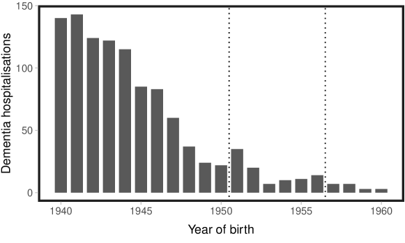
Figure A.1: Frequency of hospitalisations with dementia in the UK Biobank by birth year.

The vertical dotted lines show our approximate sample window (1950-1956).

Table A.1: Mapping between qualifications and years of education.

Qualifications	Years of education
College or university degree	16
A/AS levels $+$ NVQ/HND/HNC	14
A/AS levels $+$ Other professional qualifications	15
NVQ/HND/HNC	13
Other professional qualifications	12
A/AS levels	13
CSEs, GCSEs, or O levels	11
No qualifications	10

• Columns: (1) the qualifications recorded in the UK Biobank, (2) the assigned years of education. A plus indicates that the individual must hold both of the specified qualifications simultaneously.

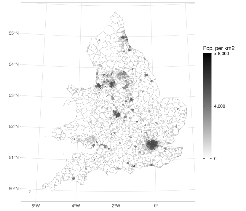
Figure A.2: Population density (in population per $\text{km}^{2}$) at the district level in England and Wales.

This map uses data provided through www.visionofbritain.org.uk and uses historical material which is copyright of the Great Britain Historical GIS Project and the University of Portsmouth [109, 112].

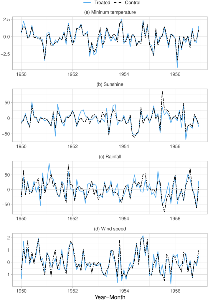
Figure A.3: Time series for minimum temperature, sunshine, rainfall, and wind speed in control and treated districts.

We take the measurements at the birth locations of all individuals in our sample and average these by year-month and treatment status. Before averaging we remove seasonality using a set of month dummies.

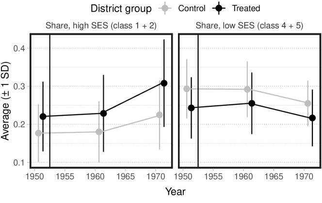
Figure A.4: Socioeconomic composition across the 1951, 1961, and 1971 censuses in control and treated districts.

Shows shares of high SES (left panel) and low SES (right panel) residents in respectively control districts (gray) and treated districts (black). Vertical black line marks 1952; the year of the London smog.

Table A.2: Impact of smog exposure on the birth locations of sibling pairs.

	Dependent variable:
	(1)	(2)
	Moved	Moved
Post	$-0.001$	$-0.003$
	$(0.018)$	$(0.034)$
Treated	$0.249^{***}$
	$(0.049)$
Treated $\times$ Post	$0.020$	$0.043$
	$(0.052)$	$(0.056)$
Age	$0.002^{***}$	$0.002^{***}$
	$(0.001)$	$(0.001)$
Observations	3,079	3,079
$R^{2}$	0.045	0.318

• Columns: (1) without fixed effects, (2) with district, year-of-birth, and month-of-birth fixed effects. (*): $p<0.1$, (**): $p<0.05$, (***): $p<0.01$.

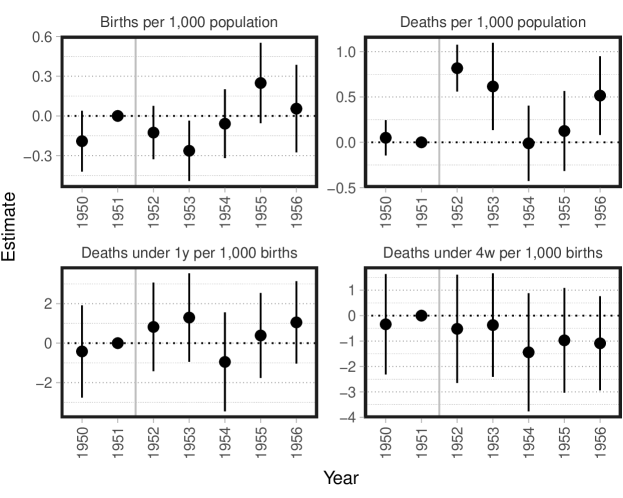
Figure A.5: Estimates from event-study specifications comparing births, mortality, mortality under age 1, and mortality under 4 weeks in treated and control districts over time.

Years to the right of the vertical line are post smog. 1951 is the reference year. The vertical lines on top of the point estimates show 0.95 confidence intervals.

Table A.3: Difference-in-Difference estimates comparing treated to control districts defined as urban England and Wales.

	Exits with highest qualification:
	(1)	(2)	(3)	(4)
	Degree	Upper secondary	Lower secondary	None
Treated $\times$ In utero	$-0.001$	$-0.022$	$0.011$	$0.012$
	$(0.019)$	$(0.017)$	$(0.012)$	$(0.011)$
Treated $\times$ Childhood	$-0.010$	$-0.018$	$0.028^{*}$	$0.001$
	$(0.019)$	$(0.018)$	$(0.015)$	$(0.011)$
In utero	$-0.016$	$0.023^{**}$	$0.000$	$-0.008$
	$(0.011)$	$(0.012)$	$(0.009)$	$(0.009)$
Childhood	$-0.017$	$0.037^{*}$	$-0.007$	$-0.013$
	$(0.023)$	$(0.022)$	$(0.017)$	$(0.017)$
Observations	64,681	64,681	64,681	64,681
Mean dep. var.	0.347	0.356	0.17	0.126
$R^{2}$	0.07	0.021	0.029	0.036

• Columns: (1) exits with university/college, (2) exits at upper secondary level (A/AS-levels, professional/vocational training), (3) exits at lower secondary level (CSEs, GCSEs, O-levels), (4) exits with no qualifications. Includes fixed-effects for district, month of birth, and year of birth. Also controls for gender, weather variation, and year-month linear time trends by administrative county. Urban England and Wales are defined as districts that had a population density above 400 individuals per km² in 1951. Standard errors are clustered by district. (*): $p<0.1$, (**): $p<0.05$, (***): $p<0.01$.

Table A.4: Difference-in-Difference estimates comparing treated to control districts defined as urban England and Wales.

	Dependent variable:
	(1)	(2)	(3)	(4)	(5)	(6)	(7)	(8)	(9)	(10)
	J00-J06	J09-J18	J20-J22	J30-J39	J40-J47	J60-J70	J80-J84	J85-J86	J90-J94	J95-J99
Treated $\times$ In utero	$0.000$	$0.012^{**}$	$-0.002$	$0.008$	$-0.002$	$0.000$	$0.003$	$-0.001$	$-0.002$	$0.004$
	$(0.003)$	$(0.005)$	$(0.004)$	$(0.007)$	$(0.004)$	$(0.001)$	$(0.002)$	$(0.001)$	$(0.002)$	$(0.003)$
Treated $\times$ Childhood	$0.003$	$0.009$	$-0.003$	$-0.012$	$-0.005$	$0.001$	$0.000$	$0.001$	$-0.002$	$0.002$
	$(0.003)$	$(0.006)$	$(0.005)$	$(0.007)$	$(0.005)$	$(0.001)$	$(0.002)$	$(0.002)$	$(0.003)$	$(0.003)$
In utero	$0.003^{*}$	$-0.006$	$-0.006^{*}$	$-0.003$	$0.004$	$0.001$	$-0.001$	$0.000$	$0.002$	$-0.003^{*}$
	$(0.002)$	$(0.004)$	$(0.003)$	$(0.004)$	$(0.003)$	$(0.001)$	$(0.001)$	$(0.001)$	$(0.002)$	$(0.002)$
Childhood	$0.004$	$-0.002$	$-0.012^{*}$	$-0.012$	$0.008$	$-0.002$	$0.001$	$-0.001$	$0.006^{**}$	$-0.001$
	$(0.004)$	$(0.007)$	$(0.006)$	$(0.009)$	$(0.006)$	$(0.002)$	$(0.002)$	$(0.002)$	$(0.003)$	$(0.003)$
Observations	64,917	64,917	64,919	64,919	64,920	64,917	64,917	64,917	64,918	64,917
Mean dep. var.	0.006	0.027	0.015	0.036	0.015	0.001	0.002	0.001	0.005	0.004
$R^{2}$	0.011	0.016	0.014	0.016	0.013	0.011	0.014	0.014	0.014	0.015

• Columns: Ever hospitalisatised due to (1) J00-J06 Acute upper respiratory infections, (2) J09-J18 Influenza and pneumonia, (3) J20-J22 Other acute lower respiratory infections, (4) J30-J39 Other diseases of upper respiratory tract, (5) J40-J47 Chronic lower respiratory diseases, (6) J60-J70 Lung diseases due to external agents, (7) J80-J84 Other respiratory diseases principally affecting the interstitium, (8) J85-J86 Suppurative and necrotic conditions of lower respiratory tract, (9) J90-J94 Other diseases of pleura, (10) J95-J99 Other diseases of the respiratory system. Includes fixed-effects for district, month of birth, and year of birth. Also controls for gender, weather variation, and year-month linear time trends by administrative county. Urban England and Wales are defined as districts that had a population density above 400 individuals per km² in 1951. Standard errors are clustered by district. (*): $p<0.1$, (**): $p<0.05$, (***): $p<0.01$.

Table A.5: Sensitivity of main difference-in-difference estimates to different sets of regressors).

	Dependent variable:
	(1)	(2)	(3)	(4)	(5)	(6)	(7)
	Educational attainment	Fluid intelligence	Respiratory, any	Influenza/ pneumonia	COVID-19	Cancer	Cardio- vascular
Panel (a) – Base
Treated $\times$ In utero	$-0.031$	$-0.070$	$0.024^{***}$	$0.007$	$0.000$	$-0.000$	$0.005$
	$(0.077)$	$(0.044)$	$(0.008)$	$(0.005)$	$(0.003)$	$(0.011)$	$(0.010)$
Treated $\times$ Childhood	$-0.060$	$-0.092^{***}$	$-0.000$	$0.003$	$-0.001$	$0.006$	$-0.003$
	$(0.047)$	$(0.033)$	$(0.008)$	$(0.004)$	$(0.001)$	$(0.007)$	$(0.008)$
In utero	$-0.047$	$0.021$	$-0.001$	$0.001$	$0.001$	$0.020^{***}$	$0.017^{***}$
	$(0.031)$	$(0.020)$	$(0.003)$	$(0.002)$	$(0.001)$	$(0.005)$	$(0.005)$
Childhood	$-0.083^{***}$	$-0.003$	$0.008^{***}$	$0.005^{***}$	$0.001$	$0.028^{***}$	$0.026^{***}$
	$(0.022)$	$(0.018)$	$(0.003)$	$(0.002)$	$(0.001)$	$(0.004)$	$(0.004)$
Observations	$64,702$	$26,934$	$64,944$	$64,938$	$65,081$	$64,947$	$64,954$
Mean dep. var.	$13.318$	$6.43$	$0.092$	$0.027$	$0.007$	$0.142$	$0.192$
$R^{2}$	$0.010$	$0.005$	$0.002$	$0.001$	$0.001$	$0.002$	$0.014$
Panel (b) – Add district FE
Treated $\times$ In utero	$-0.049$	$-0.071$	$0.024^{***}$	$0.007$	$0.000$	$0.000$	$0.005$
	$(0.076)$	$(0.043)$	$(0.008)$	$(0.005)$	$(0.003)$	$(0.011)$	$(0.010)$
Treated $\times$ Childhood	$-0.045$	$-0.086^{**}$	$-0.001$	$0.002$	$-0.001$	$0.006$	$-0.002$
	$(0.046)$	$(0.034)$	$(0.008)$	$(0.004)$	$(0.001)$	$(0.007)$	$(0.008)$
In utero	$-0.036$	$0.019$	$-0.001$	$0.000$	$0.001$	$0.020^{***}$	$0.018^{***}$
	$(0.031)$	$(0.019)$	$(0.003)$	$(0.002)$	$(0.001)$	$(0.005)$	$(0.005)$
Childhood	$-0.088^{***}$	$-0.011$	$0.009^{***}$	$0.005^{***}$	$0.001$	$0.029^{***}$	$0.026^{***}$
	$(0.021)$	$(0.019)$	$(0.003)$	$(0.001)$	$(0.001)$	$(0.004)$	$(0.004)$
Observations	$64,681$	$26,877$	$64,923$	$64,917$	$65,060$	$64,926$	$64,933$
Mean dep. var.	$13.317$	$6.429$	$0.092$	$0.027$	$0.007$	$0.142$	$0.192$
$R^{2}$	$0.076$	$0.058$	$0.014$	$0.013$	$0.011$	$0.013$	$0.027$
Panel (c) – Add time (year and month of birth) FE and trends
Treated $\times$ In utero	$-0.100$	$-0.111^{**}$	$0.019^{*}$	$0.012^{**}$	$0.000$	$-0.003$	$0.011$
	$(0.089)$	$(0.051)$	$(0.011)$	$(0.005)$	$(0.003)$	$(0.013)$	$(0.015)$
Treated $\times$ Childhood	$-0.135$	$-0.158^{**}$	$-0.007$	$0.009$	$-0.001$	$-0.001$	$0.006$
	$(0.088)$	$(0.068)$	$(0.012)$	$(0.006)$	$(0.003)$	$(0.014)$	$(0.019)$
In utero	$-0.002$	$0.008$	$-0.006$	$-0.006$	$-0.000$	$-0.005$	$-0.004$
	$(0.054)$	$(0.036)$	$(0.006)$	$(0.004)$	$(0.002)$	$(0.008)$	$(0.010)$
Childhood	$-0.014$	$-0.052$	$-0.008$	$-0.002$	$-0.001$	$-0.009$	$-0.016$
	$(0.120)$	$(0.074)$	$(0.014)$	$(0.007)$	$(0.004)$	$(0.016)$	$(0.023)$
Observations	$64,681$	$26,877$	$64,923$	$64,917$	$65,060$	$64,926$	$64,933$
Mean dep. var.	$13.317$	$6.429$	$0.092$	$0.027$	$0.007$	$0.142$	$0.192$
$R^{2}$	$0.080$	$0.067$	$0.018$	$0.016$	$0.013$	$0.016$	$0.030$
Panel (d) – Add weather covariates
Treated $\times$ In utero	$-0.100$	$-0.112^{**}$	$0.020^{*}$	$0.012^{**}$	$0.000$	$-0.003$	$0.011$
	$(0.089)$	$(0.051)$	$(0.011)$	$(0.005)$	$(0.003)$	$(0.013)$	$(0.015)$
Treated $\times$ Childhood	$-0.135$	$-0.158^{**}$	$-0.007$	$0.009$	$-0.001$	$-0.001$	$0.007$
	$(0.088)$	$(0.068)$	$(0.012)$	$(0.006)$	$(0.003)$	$(0.014)$	$(0.019)$
In utero	$-0.003$	$0.008$	$-0.005$	$-0.006$	$-0.000$	$-0.005$	$-0.004$
	$(0.054)$	$(0.036)$	$(0.006)$	$(0.004)$	$(0.002)$	$(0.008)$	$(0.010)$
Childhood	$-0.014$	$-0.051$	$-0.008$	$-0.002$	$-0.001$	$-0.009$	$-0.015$
	$(0.120)$	$(0.074)$	$(0.014)$	$(0.007)$	$(0.004)$	$(0.016)$	$(0.023)$
Observations	$64,681$	$26,877$	$64,923$	$64,917$	$65,060$	$64,926$	$64,933$
Mean dep. var.	$13.317$	$6.429$	$0.092$	$0.027$	$0.007$	$0.142$	$0.192$
$R^{2}$	$0.080$	$0.067$	$0.018$	$0.016$	$0.013$	$0.016$	$0.030$

• Columns: (1) educational attainment in years, (2) standardised fluid intelligence score, (3) ever hospitalised due to respiratory disease, (4) ever hospitalised due to influenza/pneumonia, (5) hospitalisation or death due to COVID-19, (6) ever hospitalised due to cardio-vascular disease, (7) ever hospitalised due to cancer. Panels show the estimates for increasingly complex sets of regressors. The base specification in Panel (a) only contains indicators for whether the individual was born in a treatment district and whether the individual belonged to the childhood, in utero, or after birth cohorts. Panels (b)-(d) add additional regressors to this specification. Standard errors are clustered by district. (*): $p<0.1$, (**): $p<0.05$, (***): $p<0.01$.

Table A.6: Robust estimates of average treatment effects using estimator from Borusyak et al. (2021). Compares treated to control districts defined as urban England and Wales.

	Dependent variable:
	(1)	(2)	(3)	(4)	(5)	(6)	(7)
	Educational attainment	Fluid intelligence	Respiratory, any	Influenza/ pneumonia	COVID-19	Cancer	Cardio- vascular
ATT, In utero	$-0.049$	$-0.137$	$0.025^{***}$	$0.008$	$0.000$	$0.000$	$0.004$
	$(0.075)$	$(0.089)$	$(0.009)$	$(0.005)$	$(0.003)$	$(0.011)$	$(0.011)$
ATT, Childhood	$-0.043$	$-0.161^{**}$	$-0.001$	$0.002$	$-0.000$	$0.006$	$-0.002$
	$(0.047)$	$(0.069)$	$(0.008)$	$(0.004)$	$(0.001)$	$(0.007)$	$(0.008)$

• Columns: (1) educational attainment in years, (2) standardised fluid intelligence score, (3) ever hospitalised due to respiratory disease, (4) ever hospitalised due to influenza/pneumonia, (5) hospitalisation or death due to COVID-19, (6) hospitalised due to cardio-vascular disease, (7) hospitalised due to cancer. Reports the robust estimates of the ATTs for the in utero and childhood cohorts when we assign equal weights across units in these cohorts. Includes fixed-effects for district, month of birth, and year of birth. Also controls for year-month linear time trends by administrative county. Urban England and Wales are defined as districts that had a population density above 400 individuals per km² in 1951. Standard errors are clustered by district. (*): $p<0.1$, (**): $p<0.05$, (***): $p<0.01$.

Table A.7: Difference-in-Difference estimates comparing treated to control districts defined as urban England and Wales.

	Dependent variable:
	(1)	(2)
	Educational attainment	Fluid intelligence
Treated $\times$ In utero	$-0.078$	$-0.096^{*}$
	$(0.085)$	$(0.050)$
Treated $\times$ Childhood	$-0.120$	$-0.163^{**}$
	$(0.084)$	$(0.066)$
In utero	$-0.019$	$0.003$
	$(0.053)$	$(0.035)$
Childhood	$-0.037$	$-0.057$
	$(0.118)$	$(0.072)$
Observations	65,724	27,333
Mean dep. var.	13.32	0
$R^{2}$	0.079	0.066

• Columns: (1) educational attainment in years, (2) standardised fluid intelligence score. Includes fixed-effects for district, month of birth, and year of birth. Also controls for gender, weather variation, and year-month linear time trends by administrative county. Urban England and Wales are defined as districts that had a population density above 400 individuals per km² in 1951. Standard errors are clustered by district. (*): $p<0.1$, (**): $p<0.05$, (***): $p<0.01$.

Table A.8: Difference-in-Difference estimates comparing treated to control districts defined as urban England and Wales.

	Dependent variable:
	(1)	(2)	(3)	(4)	(5)
	Respiratory, any	Influenza/ pneumonia	COVID-19	Cancer	Cardio- vascular
Treated $\times$ In utero	$0.018^{*}$	$0.011^{**}$	$0.000$	$-0.005$	$0.012$
	$(0.010)$	$(0.005)$	$(0.003)$	$(0.013)$	$(0.015)$
Treated $\times$ Childhood	$-0.009$	$0.009$	$-0.001$	$-0.005$	$0.005$
	$(0.012)$	$(0.006)$	$(0.003)$	$(0.014)$	$(0.019)$
In utero	$-0.006$	$-0.006$	$0.000$	$-0.004$	$-0.004$
	$(0.006)$	$(0.004)$	$(0.002)$	$(0.008)$	$(0.010)$
Childhood	$-0.007$	$-0.002$	$-0.001$	$-0.007$	$-0.013$
	$(0.014)$	$(0.007)$	$(0.004)$	$(0.016)$	$(0.023)$
Observations	65,977	65,971	66,117	65,980	65,987
Mean dep. var.	0.093	0.027	0.007	0.142	0.193
$R^{2}$	0.018	0.016	0.013	0.016	0.03

• Columns: (1) ever hospitalised due to respiratory disease, (2) ever hospitalised due to influenza/pneumonia, (3) hospitalisation or death due to COVID-19, (4) ever hospitalised due to cardio-vascular disease, (5) ever hospitalised due to cancer. Includes fixed-effects for district, month of birth, and year of birth. Also controls for gender, weather variation, and year-month linear time trends by administrative county. Urban England and Wales are defined as districts that had a population density above 400 individuals per km² in 1951. Standard errors are clustered by district. (*): $p<0.1$, (**): $p<0.05$, (***): $p<0.01$.

Table A.9: Difference-in-Difference estimates comparing treated to control districts defined as urban England and Wales.

	Dependent variable:
	(1)
	Male
Treated $\times$ In utero	$-0.007$
	$(0.021)$
Treated $\times$ Childhood	$0.011$
	$(0.020)$
In utero	$0.001$
	$(0.011)$
Childhood	$-0.044^{**}$
	$(0.022)$
Observations	65,060
Mean dep. var.	0.443
$R^{2}$	0.014

• Columns: (1) being born as male. Includes fixed-effects for district, month of birth, and year of birth. Also controls for gender, weather variation, and year-month linear time trends by administrative county. Urban England and Wales are defined as districts that had a population density above 400 individuals per km² in 1951. Standard errors are clustered by district. (*): $p<0.1$, (**): $p<0.05$, (***): $p<0.01$.

Table A.10: Heterogeneity across genetics – Qualifications. Difference-in-Difference estimates comparing treated to control districts defined as urban England and Wales.

	Exits with highest qualification:
	(1)	(2)	(3)	(4)
	Degree	Upper secondary	Lower secondary	None
Panel (a) – High polygenic score
Treated $\times$ In utero	$-0.036$	$-0.015$	$0.047^{***}$	$0.005$
	$(0.024)$	$(0.025)$	$(0.017)$	$(0.009)$
Treated $\times$ Childhood	$-0.017$	$-0.025$	$0.023$	$0.020^{**}$
	$(0.029)$	$(0.027)$	$(0.019)$	$(0.010)$
In utero	$-0.014$	$0.027$	$-0.015$	$0.002$
	$(0.016)$	$(0.018)$	$(0.012)$	$(0.008)$
Childhood	$-0.054$	$0.045$	$0.011$	$-0.002$
	$(0.033)$	$(0.033)$	$(0.024)$	$(0.019)$
Observations	$32,376$	$32,376$	$32,376$	$32,376$
Mean dep. var.	$0.454$	$0.337$	$0.139$	$0.07$
$R^{2}$	$0.077$	$0.039$	$0.041$	$0.039$
Panel (b) – Low polygenic score
Treated $\times$ In utero	$0.045$	$-0.029$	$-0.028$	$0.012$
	$(0.031)$	$(0.031)$	$(0.022)$	$(0.021)$
Treated $\times$ Childhood	$0.004$	$-0.008$	$0.040$	$-0.036$
	$(0.031)$	$(0.027)$	$(0.027)$	$(0.022)$
In utero	$-0.023$	$0.023$	$0.015$	$-0.016$
	$(0.014)$	$(0.016)$	$(0.014)$	$(0.014)$
Childhood	$0.012$	$0.034$	$-0.023$	$-0.023$
	$(0.029)$	$(0.032)$	$(0.026)$	$(0.028)$
Observations	$32,233$	$32,233$	$32,233$	$32,233$
Mean dep. var.	$0.24$	$0.376$	$0.202$	$0.183$
$R^{2}$	$0.069$	$0.032$	$0.040$	$0.044$

• Columns: (1) exits with university/college degree, (2) exits at upper secondary level (A/AS-levels, professional/vocational training), (2) exits at lower secondary level (CSEs, GCSEs, O-levels), (3) exits with no qualifications. Panels: (a) high PGS subsample, (b) low PGS subsample. Includes fixed-effects for district, month of birth, and year of birth. Also controls for gender, weather variation, and year-month linear time trends by administrative county. Urban England and Wales are defined as districts that had a population density above 400 individuals per km² in 1951. Standard errors are clustered by district. (*): $p<0.1$, (**): $p<0.05$, (***): $p<0.01$.

B.  Choice of time trends

The main analysis controls for administrative-county-specific (year-month) trends to allow the outcome of interest to trend differently in each administrative county. We here explore the sensitivity of the trend-specifications. Panel (a) of Table B.1, includes administrative county-specific annual (as opposed to year-month) trends. Panel (b) specifies year-month trends for each of the over 1400 districts observed in our data, and Panel (c) allows for district-specific annual trends. Finally, Panel (d) does not include any trends and only accounts for year of birth dummies.

Table B.1: Specification of trends. Difference‐in‐Difference estimates comparing treated to control districts defined as urban England and Wales.

	Dependent variable:
	(1)	(2)	(3)	(4)
	Educational attainment	Fluid intelligence	Respiratory, any	Influenza/ pneumonia
Panel (a) – Year by administrative county
Treated $\times$ In utero	$-0.087$	$-0.101^{**}$	$0.016$	$0.010^{*}$
	$(0.089)$	$(0.050)$	$(0.010)$	$(0.005)$
Treated $\times$ Childhood	$-0.119$	$-0.142^{**}$	$-0.014$	$0.007$
	$(0.086)$	$(0.066)$	$(0.012)$	$(0.006)$
Panel (b) – Year-month by district
Treated $\times$ In utero	$-0.118$	$-0.164^{***}$	$0.022^{*}$	$0.017^{***}$
	$(0.091)$	$(0.048)$	$(0.012)$	$(0.006)$
Treated $\times$ Childhood	$-0.173^{*}$	$-0.248^{***}$	$-0.003$	$0.017^{**}$
	$(0.098)$	$(0.064)$	$(0.016)$	$(0.007)$
Panel (c) – Year by district
Treated $\times$ In utero	$-0.111$	$-0.150^{***}$	$0.017$	$0.013^{**}$
	$(0.090)$	$(0.047)$	$(0.012)$	$(0.006)$
Treated $\times$ Childhood	$-0.165^{*}$	$-0.230^{***}$	$-0.013$	$0.012^{*}$
	$(0.093)$	$(0.062)$	$(0.015)$	$(0.007)$
Panel (d) – No trend
Treated $\times$ In utero	$-0.049$	$-0.072^{*}$	$0.024^{***}$	$0.008$
	$(0.075)$	$(0.043)$	$(0.008)$	$(0.005)$
Treated $\times$ Childhood	$-0.046$	$-0.086^{**}$	$-0.001$	$0.002$
	$(0.046)$	$(0.034)$	$(0.008)$	$(0.004)$

• Columns: (1) educational attainment in years, (2) standardised fluid intelligence score, (3) ever hospitalised due to respiratory disease, (4) ever hospitalised due to influenza/pneumonia. Panels: (a) Year trend at administrative county ($n=174$) level, (b) Year-month trend at district ($n=785$) level, (c) Year trend at district level. (d) No trends. We always include district FE, year-of-birth FE, and month-of-birth FE, and we always control for gender and weather variation. Standard errors are clustered by district.

The estimates are generally consistent across the different specifications. For educational attainment, we find negative estimates throughout for both in utero and childhood exposure. For fluid intelligence, we find clear evidence of a negative effect of smog exposure that is slightly larger for exposure in childhood compared to prenatally. The in utero estimates are always positive for respiratory disease, but they are slightly smaller when accounting for annual trends at either the administrative county or district level. For influenza/pneumonia, the estimates always have the same sign, but are somewhat smaller when controlling for annual trends or not including a trend. Nevertheless, for both respiratory disease and influenza/pneumonia, the magnitudes of the estimates remains in the same ballpark, suggesting that smog exposure increases the probability of being diagnosed with respiratory disease.

C.  Common time trends

Our specification implicitly assumes that individuals who were born in districts that were affected by the London smog would have had similar trends in their outcomes of interest in the absence of the smog compared to those born in districts that were not affected. To explore this common trend assumption empirically, we compare the trends in the relevant outcomes of interest among those conceived at different points in time throughout our observation period in treated and control districts. Note here, that we are mainly interested in comparing individuals in treated and control districts who are conceived after the smog, since those who are conceived before or during the smog were potentially exposed either in utero or in childhood. We here focus on our main outcomes of interest: education, fluid intelligence and respiratory disease.

Figure C.1 shows the conditional difference in the mean of the relevant outcome for those born in treated versus control districts across childhood, trimesters in utero, and 9 month intervals throughout our observation period. We condition on the same controls and fixed-effects as in the main analysis. The two vertical dotted lines indicate the threshold for potential exposure in childhood and in utero.

Figure C.1a and Figure C.1b show that those exposed in utero or in early childhood have lower education and fluid intelligence compared to those born at the same time, but in control districts. Similarly, Figure C.1c shows that those who are exposed to the smog whilst in utero have a higher probability of being diagnosed with respiratory disease compared to those born at the same time, but in control districts. For all outcomes, we see no suggestion of differential trends for those conceived after the smog, i.e., those to the right of the second vertical dotted line. In other words, we find no evidence to suggest that those born in treated districts have differential trends in our outcomes of interest compared to those born control districts.

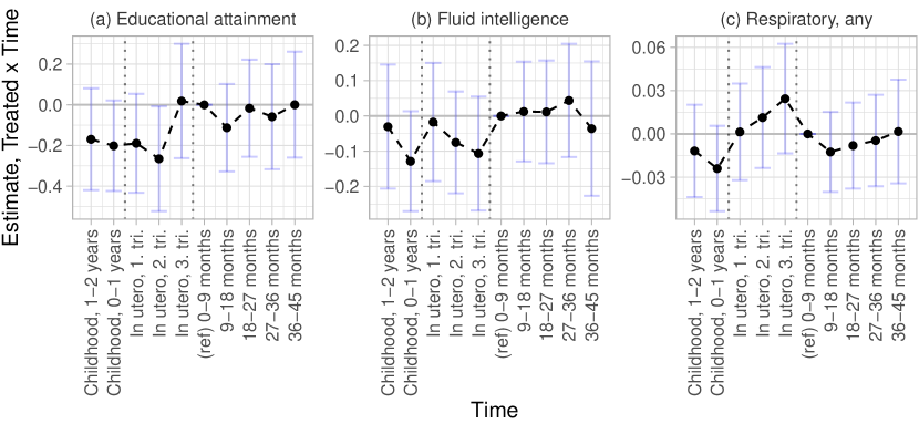
Figure C.1: The conditional differences in the means of the relevant outcome for those born in treated versus control districts.

Shows the conditional differences across childhood, trimesters in utero, and 9 month intervals throughout our observation period. We condition on the same controls as in the main analysis, and we include fixed-effects for district. We also control for gender, weather variation, and year-month linear time trends by administrative county. The two vertical dotted lines indicate the threshold for potential exposure in childhood and in utero. The vertical bars show $90\%$ confidence intervals around the point estimates. Control districts are defined as districts in England and Wales that had a population density above 400 individuals per km² in 1951. Standard errors are clustered by district.

D.  A brief background to genetics

Humans have 46 chromosomes stored in every cell apart from sex-cells. The chromosomes exist in pairs such that each pair has a maternal and paternal copy. A single chromosome consists of a double-strand of deoxyribonucleic acid (DNA) containing a large number of ‘base pairs’: pairs of nucleotide molecules (referred to as the ‘letters’ A (adenine) that binds with T (thymine), and G (guanine) that binds with C (cytosine)) that together make up the human genome. In a population there will be variation in the base pairs at some locations. Such variation is known as a single nucleotide polymorphism (SNP, pronounced ‘snip’) – a change in the base pair at one particular locus (location) – and is the most commonly studied genetic variation. When there are two possible base pairs at a given location (i.e., two alleles), the most frequent base pair is called the major allele, while the less frequent is called the minor allele. As humans have two copies of each chromosome, any given individual can have either zero, one, or two copies of the minor allele.

To identify specific SNPs that are robustly associated with a particular outcome of interest, so-called Genome-Wide Association Studies (GWAS) relate each SNP to the outcome in a hypothesis-free approach. As there are more SNPs than individuals, the SNP effects cannot be identified in a multivariate regression model. Instead, a GWAS runs a large number of univariate regressions of the outcome on each SNP. These analyses have shown that most outcomes of interest in the social sciences are ‘polygenic’: they are affected by a large number of SNPs, each with a very small effect. To increase the predictive power of the SNPs, it is therefore custom to aggregate the individual SNPs into so-called polygenic scores, as:

$$G_{i}=\sum_{j=1}^{J}\beta_{j}X_{ij},$$

where $X_{ij}$ is a count of the number of minor alleles (i.e., 0, 1 or 2) at SNP $j$ for individual $i$, and $\beta_{j}$ is its effect size obtained from an independent GWAS. Hence, the polygenic scores are weighted linear combinations of SNPs, where the weights are estimated in an independent GWAS. This is motivated by an additive genetic model where all SNPs contribute additively to the overall genetic predisposition of an individual [98, see e.g.,].

We conduct our own tailor-made GWAS for each of the main outcomes in our analysis. To avoid overfitting, we partition the UK Biobank into three non-overlapping samples: (1) a GWAS discovery sample, (2) a reference/tuning sample, and (3) the analysis sample. We use samples (1) and (2) to construct polygenic scores for the individuals in the analysis sample (i.e., sample (3)). We then use these polygenic scores to explore the extent to which one’s genetic predisposition can ‘protect’ or ‘exacerbate’ the effect of early-life pollution exposure. The analysis sample is outlined in Section 3 and contains individuals born in treated or control districts in 1950–1956. The GWAS discovery sample contains individuals born outside the study period, i.e., 1934-1949 and 1957-1970, as well as individuals born outside treated and control districts in the years 1950-1956. From the GWAS discovery sample, we randomly sample 20,000 unrelated individuals of white British ancestry that we exclusively use for the reference sample.

The GWAS discovery sample sizes and descriptive statistics are reported in Table D.1. The sample size varies depending on the outcome of interest. For our GWAS, we follow the quality control (QC) procedure described by [50] to remove genetic outliers and ensure the genotypes are well-measured. We follow the literature and include minimal covariates in the GWAS, controlling for gender, genotyping array, birth year, and the first 20 genetic principal components. To maximise the size of the discovery sample, we use BOLT-LMM [79] to run the GWAS. Since BOLT-LMM uses a linear mixed model, it allow us to include some related individuals and to relax the restrictions on ancestry (i.e., European ancestry instead of white British individuals only).

Using the GWAS estimates, we use LDPred2 [97] to construct polygenic scores. We construct the polygenic scores under both an infinitesimal model (all SNPs are causal) and a model where the proportion of causal SNPs is estimated as an additional parameter using a grid search [97, for more information, see]. To avoid overfitting, this grid search is done in the reference sample. We reduce the computational burden by including only SNPs that are in HapMap3 [8], resulting in approximately 1.6 million SNPs. We also filter the SNPs using a minor allele frequency threshold of $0.01$ and an info score threshold of $0.97$.

All polygenic scores are standardised to have zero mean and unit standard deviation in the analysis sample. To validate their predictive power, we use a linear regression model to test them against their target outcome in the analysis sample. We control for sex and the first 20 genetic principal components, and we include fixed effects for year-month of birth. We report the incremental $R^{2}$ defined as the increase in $R^{2}$ when the polygenic score is included as a covariate. Table D.2 reports the results, showing that each polygenic score is highly predictive of its outcome, with the incremental $R^{2}$ ranging between 0.1% and 10%.

Table D.1: Descriptive statistics – GWAS sample.

	Obs.	Mean	Std. dev.
	(1)	(2)	(3)
Educational attainment	$378,503$	$14.736$	$5.175$
Fluid intelligence	$138,933$	$0.065$	$0.981$
Respiratory disease	$377,577$	$0.111$	$0.314$

• Columns: (1) Number of observations in the GWAS sample. (2) Sample mean in the GWAS sample. (3) Sample standard deviation in the GWAS sample. Rows: (1) educational attainment in years, (2) standardised fluid intelligence score, (3) ever hospitalised due to respiratory disease. Fluid intelligence is standardised but during the GWAS routine a small number of individuals are discarded from the sample and this causes the mean and variance to differ slightly from zero and unity above.

Table D.2: Predictive power of polygenic scores. Linear regression estimates of the main outcomes regressed on their corresponding polygenic score.

	Dependent variable:
	(1)	(2)	(3)	(4)
	Educational attainment	Fluid intelligence	Respiratory, any	Influenza/ pneumonia
Polygenic score	$0.723^{***}$	$0.631^{***}$	$0.014^{***}$	$0.004^{***}$
	$(0.008)$	$(0.012)$	$(0.001)$	$(0.001)$
Observations	$64,681$	$26,877$	$64,923$	$64,917$
$R^{2}$	$0.112$	$0.097$	$0.005$	$0.002$
Incremental $R^{2}$	$0.100$	$0.087$	$0.002$	$0.001$

• Columns: (1) educational attainment in years, (2) standardised fluid intelligence score, (3) ever hospitalised due to respiratory disease, (4) ever hospitalised due to influenza/pneumonia. We include sex and the first 20 genetic principal components as covariates. All specifications contain year-of-birth and month-of-birth fixed effects. Standard errors are heteroskedasticity robust. The incremental $R^{2}$ is the increase in $R^{2}$ relative to a null model excluding the polygenic score. (*): $p<0.1$, (**): $p<0.05$, (***): $p<0.01$.

References

- [1] D Almond “Is the 1918 Influenza Pandemic Over? Long-Term Effects of In Utero Influenza Exposure in the Post-1940 U.S. Population” In Journal of Political Economy 114, 2006, pp. 672–712
- [2] D Almond and J Currie “Human capital development before age 5” In Handbook of Labor Economics Elsevier, 2011, pp. 1315–1486
- [3] D Almond and J Currie “Killing Me Softly: The Fetal Origins Hypothesis” In The Journal of Economic Perspectives 25, 2011, pp. 153–172
- [4] Douglas Almond, Janet Currie and Valentina Duque “Childhood circumstances and adult outcomes: Act II” In Journal of Economic Literature 56.4, 2018, pp. 1360–1446
- [5] Douglas Almond, Lena Edlund and Mårten Palme “Chernobyl’s subclinical legacy: prenatal exposure to radioactive fallout and school outcomes in Sweden” In Quarterly Journal of Economics 124.4 MIT Press, 2009, pp. 1729–1772
- [6] Douglas Almond and Bhashkar Mazumder “The 1918 influenza pandemic and subsequent health outcomes: an analysis of SIPP data” In American Economic Review 95.2, 2005, pp. 258–262
- [7] Douglas Almond and Bhashkar Mazumder “Health capital and the prenatal environment: the effect of Ramadan observance during pregnancy” In American Economic Journal: Applied Economics 3.4, 2011, pp. 56–85
- [8] David M. Altshuler et al. “Integrating common and rare genetic variation in diverse human populations” In Nature 467.7311, 2010, pp. 52–58 URL: https://doi.org/10.1038/nature09298
- [9] Eva Arceo, Rema Hanna and Paulina Oliva “Does the effect of pollution on infant mortality differ between developing and developed countries? Evidence from Mexico City” In The Economic Journal 126.591 Oxford University Press Oxford, UK, 2016, pp. 257–280
- [10] Wes Austin, Stefano Carattini, John Gomez Mahecha and Michael Pesko “COVID-19 mortality and contemporaneous air pollution” CESifo Working Paper, 2020
- [11] Paul Aveyard et al. “Association between pre-existing respiratory disease and its treatment, and severe COVID-19: a population cohort study” In The lancet Respiratory medicine Elsevier, 2021
- [12] A Ball “The long-term economic costs of the Great London Smog” In Birkbeck Working Paper 1814, 2018
- [13] Alastair Ball “Hidden costs of the Great London Smog: evidence from missing births” In Economics Bulletin 38 Birkbeck, University of London, 2018
- [14] Abhijit Banerjee, Esther Duflo, Gilles Postel-Vinay and Tim Watts “Long-run health impacts of income shocks: Wine and phylloxera in nineteenth-century France” In The Review of Economics and Statistics 92.4 MIT Press, 2010, pp. 714–728
- [15] Silvia H Barcellos, Leandro S Carvalho and Patrick Turley “Education can reduce health differences related to genetic risk of obesity” In Proceedings of the National Academy of Sciences 115.42 National Academy of Sciences, 2018, pp. E9765–E9772 DOI: 10.1073/pnas.1802909115
- [16] Daniel Barth, Nicholas W Papageorge and Kevin Thom “Genetic endowments and wealth inequality” In Journal of Political Economy 128.4 The University of Chicago Press Chicago, IL, 2020, pp. 1474–1522
- [17] BBC “London fog clears after days of chaos”, 1952 URL: http://news.bbc.co.uk/onthisday/hi/dates/stories/december/9/newsid_4506000/4506390.stm
- [18] Brian Beach and W Walker Hanlon “Coal smoke and mortality in an early industrial economy” In The Economic Journal 128.615 Wiley Online Library, 2018, pp. 2652–2675
- [19] Joel Becker et al. “Resource profile and user guide of the Polygenic Index Repository” In Nature Human Behaviour Nature Publishing Group, 2021, pp. 1–15
- [20] Jere R Behrman and Mark R Rosenzweig “Returns to birthweight” In Review of Economics and Statistics 86.2 MIT Press, 2004, pp. 586–601
- [21] M L Bell and D L Davis “Reassessment of the lethal London fog of 1952: Novel indicators of acute and chronic consequences of acute exposure to air pollution” In Environmental Health Perspectives 109, 2001, pp. 389–394
- [22] M L Bell, D L Davis and T Fletcher “A retrospective assessment of mortality from the London smog episode of 1952: The role of influenza and pollution” In Environmental Health Perspectives 112, 2004, pp. 6–8
- [23] Daniel W Belsky et al. “Genetic analysis of social-class mobility in five longitudinal studies” In Proceedings of the National Academy of Sciences 115.31 National Acad Sciences, 2018, pp. E7275–E7284
- [24] Gerard J Berg, Stephanie Hinke and Nicolai Vitt “Early life exposure to measles and later-life outcomes: Evidence from the introduction of a vaccine” In arXiv preprint arXiv:2301.10558, 2023
- [25] Gerard J Berg, Stephanie Hinke and R Adele H Wang “Prenatal Sugar Consumption and Late-Life Human Capital and Health: Analyses Based on Postwar Rationing and Polygenic Scores” In arXiv preprint arXiv:2301.09982, 2023
- [26] Gerard J Berg, Maarten Lindeboom and France Portrait “Economic conditions early in life and individual mortality” In American Economic Review 96.1, 2006, pp. 290–302
- [27] Prashant Bharadwaj, Joshua Graff Zivin, Jamie T Mullins and Matthew Neidell “Early-life exposure to the great smog of 1952 and the development of asthma” In American Journal of Respiratory and Critical Care Medicine 194.12 American Thoracic Society, 2016, pp. 1475–1482
- [28] Prashant Bharadwaj, Matthew Gibson, Joshua Graff Zivin and Christopher Neilson “Gray matters: Fetal pollution exposure and human capital formation” In Journal of the Association of Environmental and Resource Economists 4.2 University of Chicago Press Chicago, IL, 2017, pp. 505–542
- [29] Laura Bierut, Pietro Biroli, Titus J Galama and Kevin Thom “Childhood socioeconomic status moderates genetic predisposition for peak smoking” In BioRxiv Cold Spring Harbor Laboratory, 2018, pp. 336834
- [30] Govert E Bijwaard et al. “Severe Prenatal Shocks and Adolescent Health: Evidence from the Dutch Hunger Winter” In CEPR Discussion Paper No. DP16633, 2021
- [31] Pietro Biroli “Genetic and economic interaction in health formation: The case of obesity” In Working Paper, 2015
- [32] Pietro Biroli and Christian Zünd “Genes, Pubs, and Drinks: Gene-environment interplay and alcohol licensing policy in the UK” In Mimeo, University of Zurich, 2021
- [33] Pietro Biroli et al. “The economics and econometrics of gene-environment interplay” In arXiv preprint arXiv:2203.00729, 2022
- [34] Kelly C Bishop, Jonathan D Ketcham and Nicolai V Kuminoff “Hazed and confused: the effect of air pollution on dementia” In NBER Working Paper 24970, 2018
- [35] Sandra E Black, Aline Bütikofer, Paul J Devereux and Kjell G Salvanes “This is only a test? Long-run and intergenerational impacts of prenatal exposure to radioactive fallout” In Review of Economics and Statistics 101.3, 2019, pp. 531–546
- [36] Hoyt Bleakley “Disease and development: evidence from hookworm eradication in the American South” In Quarterly Journal of Economics 122.1 MIT Press, 2007, pp. 73–117
- [37] Kirill Borusyak, Xavier Jaravel and Jann Spiess “Revisiting event study designs: Robust and efficient estimation” In arXiv preprint arXiv:2108.12419, 2021
- [38] Clare Bycroft et al. “The UK Biobank resource with deep phenotyping and genomic data” In Nature 562.7726 Nature Publishing Group, 2018, pp. 203–209
- [39] Pedro Carneiro, Katrine V Løken and Kjell G Salvanes “A flying start? Maternity leave benefits and long-run outcomes of children” In Journal of Political Economy 123.2 University of Chicago Press Chicago, IL, 2015, pp. 365–412
- [40] Anne Case and Christina Paxson “Early life health and cognitive function in old age” In American Economic Review 99.2, 2009, pp. 104–09
- [41] Sarah Cattan et al. “The health effects of universal early childhood interventions: Evidence from Sure Start”, 2021
- [42] Kenneth Y Chay and Michael Greenstone “The impact of air pollution on infant mortality: evidence from geographic variation in pollution shocks induced by a recession” In Quarterly Journal of Economics 118.3 MIT Press, 2003, pp. 1121–1167
- [43] D Clark and H Royer “The effect of education on adult mortality and health: Evidence from Britain” In American Economic Review 103, 2013, pp. 2087–2120
- [44] Gabriella Conti, Giacomo Mason and Stavros Poupakis “Developmental origins of health inequality”, 2019
- [45] Flavio Cunha and James Heckman “The technology of skill formation” In American Economic Review 97.2, 2007, pp. 31–47
- [46] J Currie “Healthy, wealthy, and wise: Socioeconomic status, poor health in childhood, and human capital development” In Journal of Economic Literature 47, 2009, pp. 87–122
- [47] Janet Currie and Matthew Neidell “Air pollution and infant health: what can we learn from California’s recent experience?” In Quarterly Journal of Economics 120.3 MIT Press, 2005, pp. 1003–1030
- [48] Janet Currie and Reed Walker “Traffic congestion and infant health: Evidence from E-ZPass” In American Economic Journal: Applied Economics 3.1, 2011, pp. 65–90
- [49] N Davies et al. “The causal effects of education in the UK Biobank” In Nature Human Behaviour, 2018, pp. 117–125
- [50] BL Elsworth et al. “MRC IEU UK Biobank GWAS pipeline version 2” MRC IEU, University of Bristol., 2019 URL: https://doi.org/10.5523/bris.pnoat8cxo0u52p6ynfaekeigi
- [51] EPA “Sulfur Dioxide Basics”, 2021 URL: https://www.epa.gov/so2-pollution/sulfur-dioxide-basics
- [52] Jane Falkingham, Jo Sage, Juliet Stone and Athina Vlachantoni “Residential mobility across the life course: Continuity and change across three cohorts in Britain” In Advances in Life Course Research 30 Elsevier, 2016, pp. 111–123
- [53] Jason M Fletcher “Why have tobacco control policies stalled? Using genetic moderation to examine policy impacts.” In PloS One 7.12, 2012, pp. e50576 DOI: 10.1371/journal.pone.0050576
- [54] Jason M Fletcher “Environmental bottlenecks in children’s genetic potential for adult socio-economic attainments: Evidence from a health shock” In Population studies 73.1 Taylor & Francis, 2019, pp. 139–148
- [55] Anna Fry et al. “Comparison of sociodemographic and health-related characteristics of UK Biobank participants with those of the general population” In American Journal of Epidemiology 186.9 Oxford University Press, 2017, pp. 1026–1034
- [56] Nanna Fukushima “The UK Clean Air Act, Black Smoke, and Infant Mortality”, 2021
- [57] Joshua Graff Zivin and Matthew Neidell “Environment, health, and human capital” In Journal of Economic Literature 51.3, 2013, pp. 689–730
- [58] Michael Greenstone and B Kelsey Jack “Envirodevonomics: A research agenda for an emerging field” In Journal of Economic Literature 53.1, 2015, pp. 5–42
- [59] W Walker Hanlon “London Fog: A Century of Pollution and Mortality, 1866-1965” In Review of Economics and Statistics, 2022, pp. 1–49
- [60] W Walker Hanlon, Casper Worm Hansen and Jake Kantor “Temperature, Disease, and Death in London: Analyzing Weekly Data for the Century from 1866 to 1965” In The Journal of Economic History 81.1 Cambridge University Press, 2021, pp. 40–80
- [61] C Harmon and I Walker “Estimates of the economic return to schooling for the United Kingdom” In American Economic Review 85, 1995, pp. 1278–1286
- [62] Jennifer A Heissel, Claudia Persico and David Simon “Does pollution drive achievement? The effect of traffic pollution on academic performance” In Journal of Human Resources 57.3 University of Wisconsin Press, 2022, pp. 747–776
- [63] Hans Hersbach et al. “The ERA5 global reanalysis” In Quarterly Journal of the Royal Meteorological Society 146.730, 2020, pp. 1999–2049 DOI: https://doi.org/10.1002/qj.3803
- [64] Stephanie Hinke, Nigel Rice and Emma Tominey “Mental health around pregnancy and child development from early childhood to adolescence” In Labour Economics 78 Elsevier, 2022, pp. 102245
- [65] Adam Isen, Maya Rossin-Slater and W Reed Walker “Every breath you take—every dollar you’ll make: The long-term consequences of the clean air act of 1970” In Journal of Political Economy 125.3 University of Chicago Press Chicago, IL, 2017, pp. 848–902
- [66] Ingo E Isphording and Nico Pestel “Pandemic meets pollution: poor air quality increases deaths by COVID-19” In Journal of Environmental Economics and Management 108 Elsevier, 2021, pp. 102448
- [67] Jenny Jans, Per Johansson and J Peter Nilsson “Economic status, air quality, and child health: Evidence from inversion episodes” In Journal of Health Economics 61 Elsevier, 2018, pp. 220–232
- [68] Seema Jayachandran “Air quality and early-life mortality evidence from Indonesia’s wildfires” In Journal of Human Resources 44.4 University of Wisconsin Press, 2009, pp. 916–954
- [69] Ruixue Jia and Hyejin Ku “Is China’s pollution the culprit for the choking of South Korea? Evidence from the Asian dust” In The Economic Journal 129.624 Oxford University Press, 2019, pp. 3154–3188
- [70] David W Johnston, Carol Propper and Michael A Shields “Comparing subjective and objective measures of health: Evidence from hypertension for the income/health gradient” In Journal of Health Economics 28.3 Elsevier, 2009, pp. 540–552
- [71] Joel D Kaufman et al. “Association between air pollution and coronary artery calcification within six metropolitan areas in the USA (the Multi-Ethnic Study of Atherosclerosis and Air Pollution): a longitudinal cohort study” In The Lancet 388.10045 Elsevier, 2016, pp. 696–704
- [72] Kimin Kim and Myoung-jae Lee “Difference in differences in reverse” In Empirical Economics 57.3, 2019, pp. 705–725 DOI: 10.1007/s00181-018-1465-0
- [73] Christopher R Knittel, Douglas L Miller and Nicholas J Sanders “Caution, drivers! Children present: Traffic, pollution, and infant health” In Review of Economics and Statistics 98.2 MIT Press, 2016, pp. 350–366
- [74] Augustine Kong et al. “The nature of nurture: Effects of parental genotypes” In Science 359.6374 American Association for the Advancement of Science, 2018, pp. 424–428
- [75] The Lancet “Air pollution: a major threat to lung health”, 2019
- [76] D. Laskin “The great London smog” In Weatherwise 59, 2006, pp. 42–45
- [77] J. et al Lee “Gene discovery and polygenic prediction from a genome-wide association study of eduational attainment in 1.1 million individuals” In Nat Gen 50, 2018, pp. 1112–1121
- [78] William PD Logan “Mortality in the London fog incident, 1952.” In Lancet, 1953, pp. 336–8
- [79] Po-Ru Loh et al. “Efficient Bayesian mixed-model analysis increases association power in large cohorts” In Nature Genetics 47.3, 2015, pp. 284–290 URL: https://doi.org/10.1038/ng.3190
- [80] Lambert H Lumey, Aryeh D Stein and Ezra Susser “Prenatal famine and adult health” In Annual Review of Public Health 32 Annual Reviews, 2011, pp. 237–262
- [81] MET Office “Datasets”, 2022 URL: https://www.metoffice.gov.uk/research/climate/maps-and-data/data/haduk-grid/datasets
- [82] Melinda C Mills, Nicola Barban and Felix C Tropf “An introduction to statistical genetic data analysis” Mit Press, 2020
- [83] Ministry of Health “Mortality and morbidity during the London fog of December 1952. Reports on public health and medical subjects”, 1954
- [84] Dilnoza Muslimova et al. “Complementarities in human capital production: Evidence from genetic endowments and birth order” In arXiv preprint arXiv:2012.05021, 2020
- [85] J Peter Nilsson “Alcohol availability, prenatal conditions, and long-term economic outcomes” In Journal of Political Economy 125.4 University of Chicago Press Chicago, IL, 2017, pp. 1149–1207
- [86] John Novembre and Matthew Stephens “Interpreting principal component analyses of spatial population genetic variation” In Nature genetics 40.5 Nature publishing group, 2008, pp. 646–649
- [87] Aysu Okbay et al. “Genome-wide association study identifies 74 loci associated with educational attainment” In Nature 533.7604, 2016, pp. 539–542 URL: http://www.nature.com/doifinder/10.1038/nature17671
- [88] Aysu Okbay et al. “Polygenic prediction of educational attainment within and between families from genome-wide association analyses in 3 million individuals” In Nature Genetics 54.4 Nature Publishing Group, 2022, pp. 437–449
- [89] Rita Dias Pereira, Cornelius A Rietveld and Hans Kippersluis “The interplay between maternal smoking and genes in offspring birth weight” In Journal of Human Resources University of Wisconsin Press, 2022
- [90] Rita Dias Pereira et al. “Gene-by-Environment Interplay in the Social Sciences” In Oxford Research Encyclopedia of Economics and Finance, forthcoming
- [91] Claudia Persico “Can Pollution Cause Poverty? The effects of pollution on educational, health and economic outcomes” In Health and Economic Outcomes (February 12, 2020). American University School of Public Affairs Research Paper Forthcoming, 2020
- [92] Claudia Persico and Kathryn R Johnson “Deregulation in a time of pandemic: Does pollution increase coronavirus cases or deaths?” IZA Discussion Paper, 2020
- [93] Claudia L Persico and Joanna Venator “The effects of local industrial pollution on students and schools” In Journal of Human Resources 56.2 University of Wisconsin Press, 2021, pp. 406–445
- [94] Petra Persson and Maya Rossin-Slater “Family ruptures, stress, and the mental health of the next generation” In American Economic Review 108.4-5, 2018, pp. 1214–52
- [95] Tinca JC Polderman et al. “Meta-analysis of the heritability of human traits based on fifty years of twin studies” In Nature Genetics 47.7 Nature Publishing Group, 2015, pp. 702–709
- [96] Alkes L Price et al. “Principal components analysis corrects for stratification in genome-wide association studies” In Nature genetics 38.8 Nature Publishing Group, 2006, pp. 904–909
- [97] Florian Privé, Julyan Arbel and Bjarni J Vilhjálmsson “LDpred2: better, faster, stronger” In Bioinformatics 36.22-23 Oxford University Press, 2020, pp. 5424–5431
- [98] Shaun M. Purcell et al. “Common polygenic variation contributes to risk of schizophrenia and bipolar disorder” In Nature 460.7256, 2009, pp. 748–752 DOI: 10.1038/nature08185
- [99] Marcos A Rangel and Tom S Vogl “Agricultural fires and health at birth” In Review of Economics and Statistics 101.4 MIT Press One Rogers Street, Cambridge, MA 02142-1209, USA journals-info …, 2019, pp. 616–630
- [100] Jessica Wolpaw Reyes “Environmental policy as social policy? The impact of childhood lead exposure on crime” In The BE Journal of Economic Analysis & Policy 7.1 De Gruyter, 2007
- [101] Cornelius A Rietveld et al. “GWAS of 126,559 Individuals Identifies Genetic Variants Associated with Educational Attainment” In Science 340.6139, 2013, pp. 1467–1471 DOI: 10.1257/jep.25.4.57
- [102] Victor Ronda et al. “Family disadvantage, gender, and the returns to genetic human capital” In The Scandinavian Journal of Economics 124.2 Wiley Online Library, 2022, pp. 550–578
- [103] Michael Rutter “Genes and Behavior: Nature-Nurture Interplay Explained” Oxford Blackwell Publishing, 2006
- [104] Nicholas J Sanders “What doesn’t kill you makes you weaker prenatal pollution exposure and educational outcomes” In Journal of Human Resources 47.3 University of Wisconsin Press, 2012, pp. 826–850
- [105] Nicholas J Sanders and Charles Stoecker “Where have all the young men gone? Using sex ratios to measure fetal death rates” In Journal of Health Economics 41 Elsevier, 2015, pp. 30–45
- [106] Lauren L Schmitz and Dalton C Conley “The Long-Term Consequences of Vietnam-Era Conscription and Genotype on Smoking Behavior and Health” In Behavior Genetics 46.1 Springer US, 2016, pp. 43–58 DOI: 10.1007/s10519-015-9739-1
- [107] Lauren L Schmitz et al. “The impact of late-career job loss and genetic risk on body mass index: Evidence from variance polygenic scores” In Scientific Reports 11.1 Nature Publishing Group UK London, 2021, pp. 7647
- [108] H. R. Southall, P. Arrett, E. M. Mooney and C. Galley “Great Britain Historical Database : Health and Health Care Data : Mortality Statistics, 1851-1973.” UK Data Service., 2004
- [109] Humphrey Southall “Rebuilding the Great Britain Historical GIS, Part 1: Building an indefinitely scalable statistical database” In Historical Methods: A Journal of Quantitative and Interdisciplinary History 44.3 Taylor & Francis, 2011, pp. 149–159
- [110] Humphrey Southall and Paula Aucott “A vision of Britain through time” Department of Geography, University of Portsmouth. University of Portsmouth, 2009 URL: http://www.visionofbritain.org.uk
- [111] Eric Turkheimer “Three laws of behavior genetics and what they mean” In Current Directions in Psychological Science 9.5 SAGE Publications Sage CA: Los Angeles, CA, 2000, pp. 160–164
- [112] University of Portsmouth “Great Britain Historical GIS Project”, 2011 URL: https://www.visionofbritain.org.uk/
- [113] G van den Berg, S Hinke and A Wang “Prenatal Sugar Consumption and Late-Life Health: Analyses Based on Post-Wartime Rationing and Polygenic Scores” In mimeo, University of Bristol, 2021
- [114] Bjarni J Vilhjálmsson et al. “Modeling linkage disequilibrium increases accuracy of polygenic risk scores” In The American Journal of Human Genetics 97.4 Elsevier, 2015, pp. 576–592
- [115] S. von Hinke and N. Vitt “Accuracy of retrospective birth location data – An analysis based on siblings” In Mimeo, University of Bristol, 2023
- [116] Stephanie von Hinke, George L Wehby, Sarah Lewis and Luisa Zuccolo “Alcohol exposure in utero and child academic achievement” In The Economic Journal 124.576 Oxford University Press Oxford, UK, 2014, pp. 634–667
- [117] Warren Spring Laboratory “The investigation of Atmospheric Pollution 1958–1966: Thirty-second report” Her Majesty’s Stationery Office, London, 1967
- [118] ET Wilkins “Air pollution and the London fog of December, 1952” In Journal of the Royal Sanitary Institute 74.1 Sage Publications Sage CA: Thousand Oaks, CA, 1954, pp. 1–21
- [119] Xin Zhang, Xi Chen and Xiaobo Zhang “The impact of exposure to air pollution on cognitive performance” In Proceedings of the National Academy of Sciences 115.37 National Acad Sciences, 2018, pp. 9193–9197