SPT indices emerging from translation invariance in two-dimensional quantum spin systems

Abstract

We consider SPT-phases with on-site $G$ (where $G$ is any finite group) symmetry for two-dimensional quantum spin systems. We then impose translation invariance in one direction and observe that on top of the $H^{3}(G,\mathbb{T})$-valued index constructed in [10], an additional $H^{2}(G,\mathbb{T})$-valued index emerges. We also show that if we impose translation invariance in two directions, on top of the expected $H^{3}(G,\mathbb{T})\oplus H^{2}(G,\mathbb{T})\oplus H^{2}(G,\mathbb{T})$ valued index, an additional $H^{1}(G,\mathbb{T})$-valued index emerges.

1 Introduction

In 2010, Chen, Gu and Wen [4] introduced the notion of symmetry-protected topological phases of matter (SPT). They first considered one dimensional matrix product states and later on, Chen, Liu and Wen [5], extended this to two dimensional projective entangled pair models. Afterwards, in [3] this was extended to other dimensions. This last reference used a setup involving so-called lattice nonlinear sigma models and provided an $H^{d+1}(G,U(1))$ valued index for any $d$-dimensional lattice nonlinear sigma model. Another possible setup in which one can define SPT phases is in quantum spin systems (defined in section 2.1). In order to define SPT phases in this setting, one needs to fix a finite group $G$ with an on-site group action $g\mapsto U_{g}$ (with $g\in G$), defining a global group action $\beta_{g}$ (also defined in section 2.1). A state $\omega$, is then called $G$-invariant, if $\omega\circ\beta_{g}=\omega$. Afterwards, one needs to impose a restriction on the space of states. We ask that our states are short range entangled (SRE), see definition 2.2. A state $\omega$ is short range entangled if there is a disentangler $\gamma$. This is a locally generated automorphism, produced by a one parameter family of interactions $\Phi\in\mathcal{B}_{F_{\phi}}([0,1])$ ($\gamma=\gamma_{0;1}^{\Phi}$ as defined in section 2.3) satisfying that $\omega\circ\gamma$ is a product state. Combining these two definitions, we say that $\omega$ is an SPT state if it is short range entangled and $G$-invariant.

One then defines an equivalence relation on these SPT states by saying that $\omega_{1}$ is equivalent to $\omega_{2}$ with respect to the on site group action $U$ if there exists a $G$-invariant one parameter family of interactions $\Phi\in\mathcal{B}_{F_{\phi}}([0,1])$ such that $\omega_{1}\circ\gamma^{\Phi}_{0;1}=\omega_{2}$ (again, see section 2.3 for the definitions). One can then extend this equivalence to the stronger notion of being stably equivalent. This goes as follows: one defines an operation called stacking that takes two SPT states $\omega_{1}$ and $\omega_{2}$ and outputs a third one $\omega_{1}\otimes_{\text{stack}}\omega_{2}$ (and similarly for the group action). This $\otimes_{\text{stack}}$ is defined in section 2.1. In short, it is the tensor product at the level of the on site Hilbert space. One then defines another equivalence relation and says that two SPT states with on site group actions $(\omega_{1},U_{1})$ and $(\omega_{2},U_{2})$ are stably equivalent if and only if there exist trivial SPTs with their group actions, $(\phi_{1},\tilde{U}_{1})$ and $(\phi_{2},\tilde{U}_{2})$ and a ($G$ independent) unitary $V$ mapping between the respective on site Hilbert spaces, such that

1. $V^{\dagger}U_{1,g}\otimes\tilde{U}_{1,g}V=U_{2,g}\otimes\tilde{U}_{2,g}$ for all $g\in G$.

2. $\omega_{1}\otimes_{\text{stack}}\phi_{1}\circ i_{V}$ (where $i_{V}$ is again defined in section 2.1) is equivalent to $\omega_{2}\otimes_{\text{stack}}\phi_{2}$ with respect to the above on site group action.

In one spatial dimension so called matrix product states ([5],[11],[12]) can be used to construct non-trivial SPT states. Later on and more generally it was shown in [9] that any $G$-invariant state satisfying the split property (this includes any SRE state) carries an $H^{2}(G,\mathbb{T})$-valued index and that this index is constant on the (stable) equivalence classes. Later on in [6] it was then shown that this classification problem is complete (the index, seen as a map from the set of stable equivalence classes to $H^{2}(G,\mathbb{T})$ is injective.). In two spatial dimensions, more recently in [10], it was proven there is an $H^{3}(G,\mathbb{T})$-valued index that is constant on the (stable) equivalence classes.

We’ve used stacking to define the stable equivalence relation. Stacking however plays a more general role. It widely believed that it allows us to define an (abelian) group structure on the set of stable equivalence classes. Although it is nowhere stated explicitly, the author thinks that the literature (like for example [6]) suggests the following conjecture:

Conjecture 1.1.

Let $S$ be the set of stable SPT classes for some fixed group and a fixed lattice. Let $*$ be the map

$$*:S^{2}\rightarrow S:(\expectationvalue{\omega_{1},U_{1}}_{\sim},\expectationvalue{\omega_{2},U_{2}}_{\sim})\mapsto\expectationvalue{\omega_{1}\otimes_{\text{stack}}\omega_{2},U_{1}\otimes U_{2}}_{\sim}.$$ (1.1)

Then $*$ is well defined (independent of the choice of representative) and $S$ together with the $*$ operation forms an abelian group.

Before proceeding, we make three remarks on this conjecture:

1. The claim that $*$ is well defined and abelian is trivial. Namely, by letting $i_{V}$ be the automorphism that exchanges the two algebras that are being stacked, one can exchange the order of the stacking freely. By using

   $$\omega_{1}\circ\gamma^{\Phi_{1}}_{0;1}\otimes_{\text{stack}}\omega_{2}\circ\gamma^{\Phi_{2}}_{0;1}=(\omega_{1}\otimes_{\text{stack}}\omega_{2})\circ\gamma^{\Phi_{1}\otimes\mathbbm{1}+\mathbbm{1}\otimes\Phi_{2}}_{0;1}\sim\omega_{1}\otimes_{\text{stack}}\omega_{2},$$ (1.2)

   one can show that this is a well-defined map.

2. A representative of the inverse is sometimes called a $G$-inverse.

3. From a category point of view, if one assumes that this conjecture is true (for some subclass of groups that is a category), it is not hard to see that it gives rise to a contravariant functor from this category of groups to the category of abelian groups (say $S[G]$). More specifically, to each group morphism $f:G_{1}\rightarrow G_{2}$, one can find a group morphism $\tilde{f}:S[G_{2}]\rightarrow S[G_{1}]:\expectationvalue{\omega,U}_{\sim}\mapsto\expectationvalue{\omega,U\circ f}_{\sim}$ and this $\tilde{f}$ is indeed invariant on the choice of representative (if two states can be connected while preserving the symmetry action $\beta$, they can certainly be connected while preserving the symmetry $\beta\circ f$).

In what follows, we will call $S$ with the above group structure the stable SPT classification. In this paper we consider the 2D case with the (stable) equivalence relation as presented here but with one notable difference. We will only consider states, interactions and on site symmetries that have a translation symmetry in one direction. There is a conjecture about the SPT classification of such states, see section 3.1.5.1 of [13] for a more general and detailed exposition (which was partially based on [3]).

Conjecture 1.2.

The set of translation invariant SPTs under stable equivalence also satisfies conjecture 1.1. Let $g$ be the inclusion map from the space of 2d translation invariant SPT states to the more general set of 2d SPT states. Let $f$ be the map that takes a 1d SPT state and outputs a translation invariant 2d SPT state by taking the tensor product in the direction of the translation symmetry. The sequence

$$0\rightarrow\{\text{1d SPT states}\}\stackrel{{\scriptstyle f}}{{\rightarrow}}\{\text{2d translation invariant SPT states}\}\stackrel{{\scriptstyle g}}{{\rightarrow}}\{\text{2d SPT states}\}\rightarrow 0$$ (1.3)

induces a sequence (of group morphisms) on the stable equivalence classes. By this we mean that the class of $f(\phi)$ only depends on the class of $\phi$ and similarly for $g$. Moreover this induced sequence is exact and split.

Clearly this implies that

$$\{\text{2d translation invariant SPT classification}\}\simeq\{\text{1d SPT classification}\}\oplus\{\text{2d SPT classification}\}.$$ (1.4)

Since a 1d SPT state carries an $H^{2}(G,\mathbb{T})$ valued index and a 2d SPT state carries an $H^{3}(G,\mathbb{T})$ valued index, this means that 2d SPT states with a translation symmetry should carry an $H^{2}(G,\mathbb{T})\oplus H^{3}(G,\mathbb{T})$ valued index. This is consistent with the result of section XII of [3].

The first result of this paper is the construction of an $H^{2}(G,\mathbb{T})$ valued index (which we will denote by Index) on the space of translation invariant SPT states that is consistent with conjectures 1.1 and 1.2. By being consistent with the conjecture it is meant (among other things) that, if $\textrm{Index}_{1}$ is the one dimensional SPT index from [9], then $\textrm{Index}(f(\omega))=\textrm{Index}_{1}(\omega)$ for any 1d SPT $\omega$. This construction highly relies on the objects that are present in the construction of the 2d SPT index in [10].

We also look at the case where there is a second translation symmetry (so the system is translation invariant in both $x$ and $y$ directions). For such systems there is the following conjecture conjecture (see again [13] and [3]):

Conjecture 1.3.

The space of SPTs, translation invariant in two directions under stable equivalence also satisfies conjecture 1.1. Let $g$ be the inclusion map from the space of 2d SPT states that are translation invariant in both $x$ and $y$ directions to the more general set of 2d SPT states with translation invariance in the $x$ direction only. Let $f$ be the map that takes a 1d translation invariant SPT state and outputs a 2d SPT state that is translation invariant in both $x$ and $y$ directions by taking the tensor product in the $y$ direction. The sequence

$$0\rightarrow\mathopen{}\mathclose{{}\left\{\begin{matrix}\text{1d translation invariant}\\ \text{SPT states}\end{matrix}}\right\}\stackrel{{\scriptstyle f}}{{\rightarrow}}\mathopen{}\mathclose{{}\left\{\begin{matrix}\text{2d SPT states with two}\\ \text{translation symmetries}\end{matrix}}\right\}\stackrel{{\scriptstyle g}}{{\rightarrow}}\mathopen{}\mathclose{{}\left\{\begin{matrix}\text{2d SPT states translation}\\ \text{invariant in $x$ direction}\end{matrix}}\right\}\rightarrow 0$$ (1.5)

induces a sequence (of group morphisms) on the stable equivalence classes. By this we mean that the class of $f(\phi)$ only depends on the class of $\phi$ and similarly for $g$. Moreover, this induced sequence is exact and split.

Translation invariant SPT states in one spatial dimension are known to carry an $H^{2}(G,\mathbb{T})\oplus H^{1}(G,\mathbb{T})$ valued index (see appendix H). From this and the last two conjectures, we expect there is an

$$H^{3}(G,\mathbb{T})\oplus H^{2}(G,\mathbb{T})\oplus H^{2}(G,\mathbb{T})\oplus H^{1}(G,\mathbb{T})$$ (1.6)

valued index. The first part of the index is just $\textrm{Index}_{2d}$. The following two parts can be related to the case of a single translation symmetry as follows. Let $\mu$ be the automorphism that rotates the lattice by 90° and let $\textrm{Index}(\omega)$ be the index as constructed before (this is the second part of 1.6). The third part of the index is now given by $\textrm{Index}(\omega\circ\mu)$ (the state rotated by 90°). The last part of the index requires a different construction altogether. It can be thought of as being the charge in the Brillouin zone.

A final remark:

Remark 1.4.

As noticed in [3]. The groups in which these indices take values can be concisely written out. Using that

$$H^{0}(\mathbb{Z},\mathbb{T}) \cong\mathbb{T} H^{1}(\mathbb{Z},\mathbb{T}) \cong\mathbb{T} H^{2}(\mathbb{Z},\mathbb{T}) \cong 0 H^{3}(\mathbb{Z},\mathbb{T}) \cong 0$$ (1.7)

and inserting this into the Künneth formula for $\mathbb{Z}\times G$ gives

$$H^{2}(\mathbb{Z}\times G,\mathbb{T}) \cong\bigoplus_{i=0}^{2}H^{i}(\mathbb{Z},\mathbb{T})\otimes H^{2-i}(G,\mathbb{T})\cong H^{2}(G,\mathbb{T})\oplus H^{1}(G,\mathbb{T})$$ (1.8)

$$H^{3}(\mathbb{Z}\times G,\mathbb{T}) \cong\bigoplus_{i=0}^{3}H^{i}(\mathbb{Z},\mathbb{T})\otimes H^{3-i}(G,\mathbb{T})\cong H^{3}(G,\mathbb{T})\oplus H^{2}(G,\mathbb{T}).$$ (1.9)

This result can in turn be used to work out the Künneth formula for $\mathbb{Z}^{2}\times G$

$$H^{3}(\mathbb{Z}^{2}\times G,\mathbb{T})\cong\bigoplus_{i=0}^{3}H^{i}(\mathbb{Z},\mathbb{T})\otimes H^{3-i}(\mathbb{Z}\times G,\mathbb{T})\cong H^{3}(G,\mathbb{T})\oplus H^{2}(G,\mathbb{T})\oplus H^{2}(G,\mathbb{T})\oplus H^{1}(G,\mathbb{T}).$$ (1.10)

The layout of this paper is as follows: First in section 2 we explain the setup, define the concept of locally generated automorphisms and give the algebraic definition of group cohomology. In section 3.2 we state the two results for SRE states. In section 3.1, we state the first result using the weaker assumption 3.2 and the second result using the weaker assumption 3.5. It is using these weaker assumptions that we then prove the statements. Section 4 provides a proof of the first statement whereas section 5 provides a proof of the second statement. The results in this paper rely heavily on the methods that where developed in [10].

Acknowledgements

T.J. was supported in part by the FWO under grant G098919N.

We are grateful to the referees of Communications in Mathematical Physics for their constructive input during the review process. For example, we are very grateful for the proposed changes of lemma A.3 and the mistake in subsection 4.4 (the previous assumption was too weak).

Data availability statement

No new data were created or analyzed in this study. Data sharing is not applicable to this article.

2 Setup and definitions

In this paper we work in the two dimensional lattice $\mathbb{Z}^{2}$. We will first need some specific subsets of $\mathbb{Z}^{2}$, so let

$$L \vcentcolon=\mathopen{}\mathclose{{}\left\{(x,y)\in\mathbb{Z}^{2}\mathopen{}\mathclose{{}\left|x<0}\right.}\right\}, R \vcentcolon=\mathopen{}\mathclose{{}\left\{(x,y)\in\mathbb{Z}^{2}\mathopen{}\mathclose{{}\left|x\geq 0}\right.}\right\}$$ (2.1)

$$U \vcentcolon=\mathopen{}\mathclose{{}\left\{(x,y)\in\mathbb{Z}^{2}\mathopen{}\mathclose{{}\left|y\geq 0}\right.}\right\}, D \vcentcolon=\mathopen{}\mathclose{{}\left\{(x,y)\in\mathbb{Z}^{2}\mathopen{}\mathclose{{}\left|y<0}\right.}\right\}$$ (2.2)

be the left, right, upper and lower half planes respectively and let

$$C_{\theta}\vcentcolon=\mathopen{}\mathclose{{}\left\{(x,y)\in\mathbb{Z}^{2}\mathopen{}\mathclose{{}\left|\tan(\theta)\leq\absolutevalue{\frac{y}{x}}}\right.}\right\}$$ (2.3)

be the horizontal cone (the green area in figure 1). We will use $\tau$ to denote the bijection that moves every element of $\mathbb{Z}^{2}$ one site upward. Similarly we let $\nu$ denote the bijection that translates every element of $\mathbb{Z}^{2}$ by one site to the right. In what follows we will sometimes need to widen our cone or other subsets of $\mathbb{Z}^{2}$ vertically by one site. For this purpose we define $W$ such that for any $\Gamma\subset\mathbb{Z}^{2}$,

$$W(\Gamma)\vcentcolon=\Gamma\cup\tau(\Gamma)\cup\tau^{-1}(\Gamma).$$ (2.4)

For example, the red area in figure 1 is $W(C_{\theta})^{c}$. In the later part we will also need to rotate our lattice by $90^{\circ}$ (clockwise) so call $\mu$ the bijection on $\mathbb{Z}^{2}$ that does precisely this. Finally we will need to define the horizontal lines and the finite horizontal line

$$L_{j} \vcentcolon=\{(i,j)|i\in\mathbb{Z}\} L_{j}^{n} \vcentcolon=\{(i,j)|i\in\mathbb{Z}\cap[-n,n]\}.$$ (2.5)

2.1 Quasi local $C^{*}$-algebra

The setup in this paper will be very similar to the setup in [10] and is just the standard setup for defining quantum spin systems. For the rest of this paper, take $d\in\mathbb{N}_{+}$ arbitrary. This number will be called the on site dimension. For each $z\in\mathbb{Z}^{2}$, let $\mathcal{A}_{\{z\}}$ be an isomorphic copy of $\mathcal{B}(\mathbb{C}^{d})$ (the bounded operators on $\mathbb{C}^{d}$). In what follows, let $\mathfrak{G}_{\mathbb{Z}^{2}}$ be the set of finite subsets of $\mathbb{Z}^{2}$. For any $\Lambda\in\mathfrak{G}_{\mathbb{Z}^{2}}$, we set $\mathcal{A}_{\Lambda}=\bigotimes_{z\in\Lambda}\mathcal{A}_{\{z\}}$. We define the local algebra as $\mathcal{A}_{\text{loc}}=\bigcup_{\Lambda\in\mathfrak{G}_{\mathbb{Z}^{2}}}\mathcal{A}_{\Lambda}$ and define the quasi local $C^{*}$ algebra as the norm closure of the local algebra ($\mathcal{A}=\overline{\mathcal{A}_{\text{loc}}}$). Similarly, for any (possibly infinite) subset $\Gamma\subset\mathbb{Z}^{2}$ we set $\mathcal{A}_{\text{loc},\Gamma}=\bigcup_{\Lambda\in\mathfrak{G}_{\Gamma}}\mathcal{A}_{\Lambda}$ and $\mathcal{A}_{\Gamma}=\overline{\mathcal{A}_{\text{loc},\Gamma}}$.

Throughout this paper we will sometimes require a stronger form of locality than merely being in the norm completion of the local algebra. Specifically when $\Gamma=L_{j}$ is a horizontal line. We will say that an operator $A\in\mathcal{A}_{L_{j}}$ is summable if and only if there exists a sequence $A_{n}\in\mathcal{A}_{L_{j}^{n}}$ on the finite horizontal lines such that

$$\sum_{i=0}^{\infty}\norm{A-A_{n}}<\infty.$$ (2.6)

We will need to define some automorphisms on this algebra using the bijections defined previously. To this end, define the isomorphisms

$$\tau :\mathcal{A}_{\Gamma}\rightarrow\mathcal{A}_{\tau(\Gamma)} \nu :\mathcal{A}_{\Gamma}\rightarrow\mathcal{A}_{\nu(\Gamma)} \mu :\mathcal{A}_{\Gamma}\rightarrow\mathcal{A}_{\mu(\Gamma)}$$ (2.7)

as the translation upwards, the translation to the right and the right-handed rotation respectively. By construction, these isomorphisms are automorphisms if $\Gamma$ is taken to be $\mathbb{Z}^{2}$ (because $d$ is a constant throughout the lattice). Clearly if $\Gamma=\mathbb{Z}$ (by which we mean again the $x$-axis $(\mathbb{Z},0)$) only one of these translation automorphisms descends to an automorphism on $\mathcal{A}_{\mathbb{Z}}$. This automorphism is then also simply denoted as $\nu$.

We will need to define one additional set of automorphisms. For any set of unitaries $V_{i}\in\mathcal{U}(\mathbb{C}^{d})$ (labelled by $i\in\mathbb{Z}^{2}$), we define the (unique) automorphism $i_{V}^{\Gamma}\in\textrm{Aut}\mathopen{}\mathclose{{}\left(\mathcal{A}_{\Gamma}}\right)$ (for all $\Gamma\subset\mathbb{Z}^{2}$) such that

$$i_{V}^{\Gamma}(A)=\textrm{Ad}\mathopen{}\mathclose{{}\left(\otimes_{i\in I}V_{i}}\right)(A)$$ (2.8)

for all $I\subset\Gamma$ finite and $A\in\mathcal{A}_{I}$. More specifically, let $G$ be a finite group and let $U_{i}\in\hom(G,\mathcal{U}(\mathcal{A}_{i}))$ (for $i\in\mathbb{Z}^{2}$) be the on site group action. Let $\beta^{\Gamma}\in\hom(G,\textrm{Aut}\mathopen{}\mathclose{{}\left(\mathcal{A}_{\Gamma}}\right))$ (for any $\Gamma\subset\mathbb{Z}^{2}$) be such that

$$\beta^{\Gamma}_{g}(A)=i_{U(g)}^{\Gamma}=\textrm{Ad}\mathopen{}\mathclose{{}\left(\otimes_{i\in I}U_{i}(g)}\right)(A)$$ (2.9)

for any $g\in G$, $I\subset\Gamma$ finite and $A\in\mathcal{A}_{I}$. Clearly, any unitary transformation of our representation $U(\cdot)\rightarrow V^{\dagger}U(\cdot)V$ induces a transformation of the group action $\beta_{g}\rightarrow i_{V}^{-1}\circ\beta_{g}\circ i_{V}$.

Throughout our paper when we are discussing translation invariance in the vertical direction we will ask that the group action is translation invariant in the vertical direction ($\tau\circ\beta_{g}^{\Gamma}=\beta_{g}^{\tau(\Gamma)}\circ\tau$). If we also have translation invariance in the horizontal direction, we will also ask that the group action be translation invariant in that direction as well ($\nu\circ\beta_{g}^{\Gamma}=\beta_{g}^{\nu(\Gamma)}\circ\nu$). As it turns out, in showing that the $H^{1}$-valued index is consistent with all the conjectures of the introduction, we will even require that the on site group action $U_{i}(g)$ is the same at each site. In what follows we will always assume this. This means that when we denote an on site symmetry action we merely have to give one representation $U\in\hom(G,\mathcal{U}(\mathbb{C}^{d}))$ and when we denote a unitary transformation of the on site Hilbert space we only have to give a single unitary $V\in\mathcal{U}(\mathbb{C}^{d})$, we will use this notation frequently.

Clearly by construction there is a tensor product operation on this $C^{*}$ algebra in the sense that for any $\Gamma_{1},\Gamma_{2}\subset\mathbb{Z}^{2}$ satisfying that $\Gamma_{1}\cap\Gamma_{2}=\emptyset$ we can define a bilinear, surjective map

$$\otimes:\mathcal{A}_{\Gamma_{1}}\times\mathcal{A}_{\Gamma_{2}}\rightarrow\mathcal{A}_{\Gamma_{1}\cup\Gamma_{2}}.$$ (2.10)

There is however a second tensor product operation on this $C^{*}$ algebra that we will use. We will call it the stacking operation. It is such that for any $\Gamma\subset\mathbb{Z}^{2}$ we define the bilinear, surjective map

$$\otimes_{\text{stack}}:\mathcal{A}_{\Gamma}\times\mathcal{A}_{\Gamma}\rightarrow\mathcal{A}^{2}_{\Gamma}$$ (2.11)

where $\mathcal{A}^{2}$ is the quasi local $C^{*}$ algebra on $\mathbb{Z}^{2}$ constructed from an on site algebra $\mathcal{B}(\mathbb{C}^{d})\otimes\mathcal{B}(\mathbb{C}^{d})\simeq\mathcal{B}(\mathbb{C}^{d\times d})$. We will also need to define the stacking of the group action by which we mean

$$(\beta_{g}\otimes_{\text{stack}}\beta_{g})^{\Lambda}=\bigotimes_{z\in\Lambda}\textrm{Ad}\mathopen{}\mathclose{{}\left(U(g)\otimes U(g)_{z}}\right)$$ (2.12)

for any $\Lambda\in\mathfrak{G}_{\mathbb{Z}^{2}}$ (in fact stacking can be defined for any automorphism, not just the group action).

2.2 States on $\mathcal{A}$

We say that a linear functional $\omega:\mathcal{A}\rightarrow\mathbb{C}$ is a state if it positive and normalized. This means that for any $A\in\mathcal{A}$, $\omega(A^{\dagger}A)\geq 0$ and that $\omega(\mathbbm{1})=1$. We denote the set of states on $\mathcal{A}$ by $\mathcal{S}(\mathcal{A})$. In this paper we will work exclusively with states that are pure. In this setting, $\omega\in\mathcal{S}(\mathcal{A})$ being pure means that it is extremal in the sense that for any $p\in]0,1[$, the only two other states $\omega_{1},\omega_{2}\in\mathcal{S}(\mathcal{A})$ that satisfy

$$\omega=p\omega_{1}+(1-p)\omega_{2}$$ (2.13)

must satisfy $\omega_{1}=\omega_{2}=\omega$. The set of pure states on $\mathcal{A}$ will be called $\mathcal{P}(\mathcal{A})$. In this paper we will often refer to the GNS triple. For its definition, construction and properties we refer to [2]. We will sometimes write the tensor product of states $\omega\otimes\phi$ to be such that $(\omega\otimes\phi)(a\otimes b)=\omega(a)\phi(b)$ and similarly for the stacking tensor product. We will call a pure state $\phi$ on $\mathcal{A}_{\Gamma}$ a product state if for any $\Lambda\subset\Gamma$, the restriction $\phi|_{\mathcal{A}_{\Lambda}}$ is still pure.

We will call a state $\omega$, $G$-invariant if $\omega\circ\beta_{g}=\omega$ (where $\beta_{g}=i_{U(g)}$ with $U$ an on site group action). Moreover, let $U$ we say that a $G$-invariant product state $\phi$ is trivial with respect to $U$ (we will sometimes denote this as $(\phi,U)$ is trivial) if $\phi(U_{i}(g))=1$ for all $i\in\mathbb{Z}^{2}$.

There is a natural way to construct a pure $G$-invariant state on the quasi local $C^{*}$-algebra over $\mathbb{Z}^{2}$, $\mathcal{A}_{\mathbb{Z}^{2}}$ using a pure $G$-invariant state on the quasi local $C^{*}$-algebra over $\mathbb{Z}$, $\mathcal{A}_{L_{0}}$.

Definition 2.1.

Let $\phi\in\mathcal{P}(\mathcal{A}_{L_{0}})$ be a state that is $G$-invariant under a group action $\beta_{g}^{L_{0}}$. Define $\phi_{i}\in\mathcal{P}(\mathcal{A}_{L_{i}})$ as $\phi_{i}:=\phi_{0}\circ\tau^{-i}$. We define the infinite tensor product state $\omega_{\phi}$ as

$$\omega_{\phi}:=\bigotimes_{j\in\mathbb{Z}}\phi_{j}.$$ (2.14)

This is a $G$-invariant pure state over $\mathbb{Z}^{2}$ that is invariant under the automorphism $\tau$.

The proof that this is a well defined state is done in definition 4.17.

2.3 Interactions and locally generated automorphisms

An interaction $\Phi$ is a map

$$\Phi:\mathfrak{G}_{\mathbb{Z}^{2}}\rightarrow\mathcal{A}_{\text{loc}}:I\mapsto\Phi(I)$$ (2.15)

where $\Phi(I)\in\mathcal{A}_{I}$ is hermitian ($\Phi(I)=\Phi(I)^{*}$). We will sometimes require a norm on the space of interactions that indicates how local an interaction acts. Take $F:\mathbb{N}\rightarrow\mathbb{R}^{+}$ any monotonically decreasing positive function then we define an $F$-norm on the space of interactions by:

$$\norm{\Phi}_{F}\vcentcolon=\sup_{x,y\in\mathbb{Z}^{2}}\frac{1}{F(\absolutevalue{x-y})}\sum_{Z\in\mathfrak{G}_{\mathbb{Z}^{2}},Z\ni x,y}\norm{\Phi(Z)}.$$ (2.16)

Following [10] we will fix a specific family of monotonically decreasing positive functions by saying that for any $0<\phi<1$ we define

$$F_{\phi}:\mathbb{R}^{+}\rightarrow\mathbb{R}^{+}:r\mapsto\frac{\exp(-r^{\phi})}{(1+r)^{4}}.$$ (2.17)

We will sometimes use the restriction of an interaction. For some $\Gamma\subset\mathbb{Z}^{2}$ we define $\Phi_{\Gamma}$ by

$$\Phi_{\Gamma}:\mathfrak{G}_{\mathbb{Z}^{2}}\rightarrow\mathcal{A}_{\text{loc}}:I\mapsto\mathopen{}\mathclose{{}\left\{\begin{matrix}\Phi(I)&\text{if }I\subset\Gamma\\ 0&\text{otherwise}.\end{matrix}}\right.$$ (2.18)

The set of interactions with this norm (for a fixed $F$) is a Banach space. One of the properties of $F$-local interactions is that they can be used to generate automorphisms. Let

$$\Phi:\mathfrak{G}_{\mathbb{Z}^{2}}\times[0,1]\rightarrow\mathcal{A}_{\text{loc}}:(I,t)\mapsto\Phi(I,t)$$ (2.19)

be a norm continuous one parameter family of interactions such that the $F$-norm is uniformly bounded ($\sup_{t\in[0,1]}\norm{\Phi(\cdot,t)}_{F}<\infty$). We will denote the set of one parameter families of interactions that satisfy this property by $\mathcal{B}_{F}([0,1])$. For any $\Phi\in\mathcal{B}_{F_{\phi}}([0,1])$, we define the locally generated automorphism (LGA) $\gamma^{\Phi}_{s;t}$ such that for any $A\in\mathcal{A}$, $\gamma^{\Phi}_{s;t}(A)$ is given as the solution to the differential equation

$$\frac{\text{d}}{\text{d}t}\gamma^{\Phi}_{s;t}(A)=-i\sum_{I\in\mathfrak{G}_{\mathbb{Z}^{2}}}\gamma^{\Phi}_{s;t}([\Phi(I,t),A])$$ (2.20)

with initial condition $\gamma^{\Phi}_{s;s}(A)=A$ (the existence of this automorphism is proven in [8]). This satisfies the condition that if $\sup_{t}\norm{\sum_{I\in\mathfrak{B}_{\mathbb{Z}^{2}}}\Phi(I,t)}<\infty$ then

$$\gamma^{\Phi}_{s;t} =\textrm{Ad}\mathopen{}\mathclose{{}\left(u^{\Phi}_{s;t}}\right) u^{\Phi}_{s;t} \vcentcolon=\mathcal{T}\exp(-i\int_{t}^{s}\text{d}s^{\prime}\sum_{I\in\mathfrak{B}_{\mathbb{Z}^{2}}}\Phi(s^{\prime},t)).$$ (2.21)

Sometimes we will say that an interaction is $G$-invariant. By this we simply mean that $\beta_{g}(\Phi(I))=\Phi(I)$ (for all $I\in\mathfrak{G}_{\mathbb{Z}^{2}}$). Similarly if we say an interaction is translation invariant we mean that $\tau(\Phi(I))=\Phi(\tau(I))$ (for all $I\in\mathfrak{G}_{\mathbb{Z}^{2}}$). It should be clear that if an interaction is $G$-invariant (translation invariant) that then the LGA it generates commutes with the group action (the translation automorphism) as well.

2.4 The stable equivalence class

We will now define a subset of these states that we will call short range entangled (SRE):

Definition 2.2.

Let $\omega\in\mathcal{P}(\mathcal{A})$. We say that $\omega$ is an SRE state if and only if there exists a $\phi\in]0,1[$ such that there exists an interaction $\Phi\in\mathcal{B}_{F_{\phi}}([0,1])$ such that $\omega\circ\gamma^{\Phi}_{0;1}$ is a product state. We then call $\gamma^{\Phi}_{0;1}$ a disentangler for $\omega$.

On the set of $G$-invariant SRE states we will now define three stable equivalence classes depending on the additional imposed symmetry:

Definition 2.3.

Take $(\omega_{1},U_{1})$ and $(\omega_{2},U_{2})$ elements of

$$S_{0}=\{(\omega,U)\in\mathcal{P}(\mathcal{A})\times\hom(G,U(\mathbb{C}^{d}))|\omega\text{ is SRE},\>\omega\circ i_{U(g)}=\omega\>\forall g\in G\}$$ (2.22)

for two algebras $\mathcal{A}_{1}$ and $\mathcal{A}_{2}$. We say that $\expectationvalue{\omega_{1},U_{1}}_{\sim}=\expectationvalue{\omega_{2},U_{2}}_{\sim}$ if and only if there exists a $\phi\in]0,1[$ such that there exists a $G$-invariant interaction $\Phi\in\mathcal{B}_{F_{\phi}}([0,1])$, trivial elements of $S_{0}$ (see subsection 2.2), $(\phi_{1},\tilde{U}_{1})$ and $(\phi_{2},\tilde{U}_{2})$ for algebras $\tilde{\mathcal{A}}_{1}$ and $\tilde{\mathcal{A}}_{2}$ respectively and an on site unitary such that

$$\omega_{1}\otimes_{\text{stack}}\phi_{1}\circ i_{V} =\omega_{2}\otimes_{\text{stack}}\phi_{2}\circ\gamma^{\Phi}_{0;1} V^{\dagger}U_{1}(g)\otimes\tilde{U}_{1}(g)V =U_{2}(g)\otimes\tilde{U}_{2}(g).$$ (2.23)

We also define similar equivalence classes $\expectationvalue{\cdot}_{\sim}^{1},\expectationvalue{\cdot}_{\sim}^{2}$ and $\expectationvalue{\cdot}_{\sim}^{3}$ on

$$S_{1} =\{(\omega,U)\in\mathcal{P}(\mathcal{A})\times\hom(G,U(\mathbb{C}^{d}))|\omega\text{ is SRE},\>\omega\circ i_{U(g)}=\omega\>\forall g\in G,\>\omega\circ\tau=\omega\}$$ (2.24)

$$S_{2} =\{(\omega,U)\in\mathcal{P}(\mathcal{A})\times\hom(G,U(\mathbb{C}^{d}))|\omega\text{ is SRE},\>\omega\circ i_{U(g)}=\omega\>\forall g\in G,\>\omega\circ\nu=\omega\}$$ (2.25)

$$S_{3} =\{(\omega,U)\in\mathcal{P}(\mathcal{A})\times\hom(G,U(\mathbb{C}^{d}))|\omega\text{ is SRE},\>\omega\circ i_{U(g)}=\omega\>\forall g\in G,\>\omega\circ\tau=\omega,\>\omega\circ\nu=\omega\}$$ (2.26)

respectively. Here we now also demand that the interactions and the trivial states are invariant under the additional translation symmetries.

2.5 (Borel) Group cohomology groups

In this paper we define the Group cohomology groups using the algebraic approach. A standard reference for Group cohomology is [1]. Let $G$ be an arbitrary finite group. For any $n\in\mathbb{N}$, let $C^{n}(G,M)$ (in principle this can be for any (left) G-module $M$ but in this paper we will always take $M=\mathbb{T}$ with the addition and the trivial group action) be the group of all functions from $G^{n}$ to $M$. We will use additive notation on this space and denote the group operator by $+$ and the inverse of an element of the group $\phi$ by $-\phi$. Now define the coboundary homomorphisms

$$\text{d}^{n+1}:C^{n}(G,M)\mapsto C^{n+1}(G,M)$$ (2.27)

such that

$$(\text{d}^{n+1}\phi)(g_{1},\cdots,g_{n+1})$$

$$=g_{1}\phi(g_{2},\cdots,g_{n+1})+\sum_{i=1}^{n}(-1)^{i}\phi(g_{1},\cdots,g_{i-1},g_{i}g_{i+1},\cdots,g_{n+1})+(-1)^{n+1}\phi(g_{1},\cdots,g_{n}).$$ (2.28)

Since $\text{d}^{n+1}\circ\text{d}^{n}=0$ this defines a cochain complex and we can define its cohomology as

$$H^{n}(G,M)=Z^{n}(G,M)/B^{n}(G,M)$$ (2.29)

where

$$Z^{n}(G,M) \vcentcolon=\ker(\text{d}^{n+1}) B^{n}(G,M) \vcentcolon=\mathopen{}\mathclose{{}\left\{\begin{matrix}0&\text{if }n=0\\ \textrm{im}(\text{d}^{n})&\text{if }n\geq 1\end{matrix}}\right..$$ (2.30)

In what follows we will denote the group action on $H^{n}(G,M)$ also in the same additive notation that we used for $C^{n}(G,M)$. This notation makes sense because of the property that for any $\phi_{1},\phi_{2}\in Z^{n}(G,M)$ we have that $\expectationvalue{\phi_{1}+\phi_{2}}_{H^{n}(G,M)}=\expectationvalue{\phi_{1}}_{H^{n}(G,M)}+\expectationvalue{\phi_{2}}_{H^{n}(G,M)}$.

Remark 2.4.

In [3], they argue that this definition of group cohomology is only the right approach for discrete groups. When we want to generalize this to any continuous group that has a well defined Haar measure we additionally have to impose that the cochains are measurable. Group cohomology with measurable cochains is sometimes called Borel Group cohomology. We believe that it should be possible to construct a Borel Group cohomology group element from SPT states protected by any locally compact Lie group. However this is beyond the scope of this paper.

3 Results

This section will contain three different parts. First we discuss the main result starting from some rather abstract assumptions. In the second part we present the claim that these assumptions are implied by some more natural assumptions relating to short range entanglement. In the last part of the section we compare our assumptions to those made in [10].

3.1 Statement of the result in terms of Q-automorphisms

      

Figure 1: These figures indicate the support area of the different automorphisms in a particular decomposition of the QAut. The angle $\theta$ needs to be smaller then or equal to what was indicated here so that the $\Theta$ and the $\eta_{g}$ (possibly after widening by one site) commute.

Similarly what was done in [10], we will define an index on the space of states that can be disentangled by a Q-automorphism. This class of automorphisms is defined as:

Definition 3.1.

Take $\alpha\in\textrm{Aut}\mathopen{}\mathclose{{}\left(\mathcal{A}}\right)$. We say that $\alpha\in\textrm{QAut}_{1}\mathopen{}\mathclose{{}\left(\mathcal{A}}\right)$ if and only if $\forall\theta\in]0,\pi/2[$ there exists an $\alpha_{L}\in\textrm{Aut}\mathopen{}\mathclose{{}\left(\mathcal{A}_{L}}\right),\alpha_{R}\in\textrm{Aut}\mathopen{}\mathclose{{}\left(\mathcal{A}_{R}}\right),V_{1}\in\mathcal{U}(\mathcal{A})$ and a $\Theta\in\textrm{Aut}\mathopen{}\mathclose{{}\left(\mathcal{A}_{W(C_{\theta})^{c}}}\right)$ such that

$$\alpha=\textrm{Ad}\mathopen{}\mathclose{{}\left(V_{1}}\right)\circ\alpha_{L}\otimes\alpha_{R}\circ\Theta.$$ (3.1)

We will often write $\alpha_{0}$ to mean $\alpha_{L}\otimes\alpha_{R}$. In this paper we will consider states that satisfy the following property (see figure 1 for the support of the automorphisms):

Assumption 3.2.

Let $\omega\in\mathcal{P}(\mathcal{A})$ be

1. such that there exists an automorphism $\alpha\in\textrm{QAut}_{1}\mathopen{}\mathclose{{}\left(\mathcal{A}}\right)$ and a product state $\omega_{0}\in\mathcal{P}(\mathcal{A})$ satisfying

   $$\omega=\omega_{0}\circ\alpha.$$ (3.2)

2. such that there exists a $\theta\in]0,\pi/2[$ for which there exists a map

   $$\tilde{\beta}:G\rightarrow\textrm{Aut}\mathopen{}\mathclose{{}\left(\mathcal{A}}\right):g\mapsto\tilde{\beta}_{g}$$ (3.3)

   satisfying

   $$\omega\circ\tilde{\beta}_{g} =\omega \tilde{\beta}_{g}=\textrm{Ad}\mathopen{}\mathclose{{}\left(V_{g,2}}\right)\circ\eta^{L}_{g}\otimes\eta^{R}_{g}\circ\beta^{U}_{g}$$ (3.4)

   for some $V_{g,2}\in\mathcal{U}(\mathcal{A}),\eta^{L}_{g}\in\textrm{Aut}\mathopen{}\mathclose{{}\left(\mathcal{A}_{C_{\theta}\cap L}}\right)$ and $\eta^{R}_{g}\in\textrm{Aut}\mathopen{}\mathclose{{}\left(\mathcal{A}_{C_{\theta}\cap R}}\right)$.

3. translation invariant ($\omega\circ\tau=\omega$).

We will also require a similar subclass of automorphisms and states on the quasi local $C^{*}$-algebra over $\mathbb{Z}$, $\mathcal{A}_{L_{0}}$. We now define the assumption

Assumption 3.3.

Take $\phi\in\mathcal{P}(\mathcal{A}_{L_{0}})$ such that

1. $\phi\circ\beta_{g}=\phi$.

2. there exist automorphisms $\tilde{\alpha}_{L}\in\textrm{Aut}\mathopen{}\mathclose{{}\left(\mathcal{A}_{L_{0}\cap L}}\right)$, $\tilde{\alpha}_{R}\in\textrm{Aut}\mathopen{}\mathclose{{}\left(\mathcal{A}_{L_{0}\cap R}}\right)$ and a summable operator $b\in\mathcal{U}(\mathcal{A}_{L_{0}})$ such that

   $$\phi_{0}=\phi\circ\textrm{Ad}\mathopen{}\mathclose{{}\left(b}\right)\circ\tilde{\alpha}_{L}\otimes\tilde{\alpha}_{R}$$ (3.5)

   is a product state.

We now state the result that using assumption 3.2 we can define an $H^{2}(G,\mathbb{T})$-valued index.

Theorem 3.4.

For any $\mathcal{A}$ satisfying the construction from section 2.1 and any choice of on site group action $U\in\hom(G,U(\mathbb{C}^{d}))$, there exists a map

$$\textrm{Index}^{\mathcal{A},U}:\{\omega\in\mathcal{P}(\mathcal{A})|\omega\text{ satisfies assumption \ref{assumption}}\}\rightarrow H^{2}(G,\mathbb{T})$$ (3.6)

that is well defined (doesn’t depend on any of the choices in assumption 3.2). This map will be consistent with conjecture 1.2 by which we mean that:

1. For any $G$ invariant and translation invariant family of interactions $\Phi\in\mathcal{B}_{F_{\phi}}([0,1])$ (for some $0<\phi<1$) we have that

   $$\textrm{Index}^{\mathcal{A},U}(\omega)=\textrm{Index}^{\mathcal{A},U}(\omega\circ\gamma^{\Phi}_{0;1}).$$ (3.7)

2. For $\phi\in\mathcal{P}(\mathcal{A}_{L_{0}})$, any a one dimensional $G$-invariant state satisfying assumption 3.3, the state $\omega_{\phi}$ as defined in definition 2.1 satisfies

   $$\textrm{Index}^{\mathcal{A}_{L_{0}},U}_{1d}(\phi)=\textrm{Index}^{\mathcal{A},U}(\omega).$$ (3.8)

3. This index is a group homomorphism under the stacking operator. By this we mean that

   $$\textrm{Index}^{\mathcal{A}^{2},U\otimes U}(\omega_{1}\otimes_{\text{stack}}\omega_{2})=\textrm{Index}^{\mathcal{A},U}(\omega_{1})+\textrm{Index}^{\mathcal{A},U}(\omega_{2}).$$ (3.9)

4. The index is independent on the choice of basis for the on site Hilbert space by which we mean that for any on site unitary $V$ we get that

   $$\textrm{Index}^{\mathcal{A},\textrm{Ad}\mathopen{}\mathclose{{}\left(V^{\dagger}}\right)(U)}(\omega\circ i_{V})=\textrm{Index}^{\mathcal{A},U}(\omega).$$ (3.10)

Proof.

This statement is proven in subsection 4.8. ∎

Figure 2: This figure indicates the support area of the different automorphisms when there are two translation directions. The angle $\theta$ still has to be smaller then or equal to what was indicated here so that the $\Theta$ and the $\eta_{g}$ commute but now we must be able to do both a horizontal and a vertical widening of the support of $\eta_{g}$.

Now we will present the assumption from which we can define the $H^{1}(G,\mathbb{T})$-valued index (see figure 2 for the support of the automorphisms).

Assumption 3.5.

Let $\omega\in\mathcal{P}(\mathcal{A})$ be

1. such that there exists an automorphism $\alpha\in\textrm{QAut}_{1}\mathopen{}\mathclose{{}\left(\mathcal{A}}\right)$ and a product state $\omega_{0}\in\mathcal{P}(\mathcal{A})$ satisfying

   $$\omega=\omega_{0}\circ\alpha.$$ (3.11)

2. such that there exists a $\theta\in]0,\pi/2[$ for which there exists a map

   $$\tilde{\beta}:G\rightarrow\textrm{Aut}\mathopen{}\mathclose{{}\left(\mathcal{A}}\right):g\mapsto\tilde{\beta}_{g}$$ (3.12)

   satisfying

   $$\omega\circ\tilde{\beta}_{g} =\omega \tilde{\beta}_{g} =\textrm{Ad}\mathopen{}\mathclose{{}\left(V_{g,2}}\right)\circ\eta^{L}_{g}\otimes\eta^{R}_{g}\circ\beta^{U}_{g}$$ (3.13)

   for some $V_{g,2}\in\mathcal{U}(\mathcal{A}),$ $\eta^{L}_{g}\in\textrm{Aut}\mathopen{}\mathclose{{}\left(\mathcal{A}_{\nu^{-1}(C_{\theta}\cap L)}}\right)$ and $\eta^{R}_{g}\in\textrm{Aut}\mathopen{}\mathclose{{}\left(\mathcal{A}_{\nu(C_{\theta}\cap R)}}\right)$.

3. translation invariant in both directions

   $$\omega\circ\tau =\omega \omega\circ\nu =\omega.$$ (3.14)

Similar to before, we also require an assumption for states on the quasi local $C^{*}$-algebra over $\mathbb{Z}$.

Assumption 3.6.

Take $\phi\in\mathcal{P}(\mathcal{A}_{L_{0}})$ such that

1. $\phi\circ\beta_{g}=\phi$.

2. there exist automorphisms $\tilde{\alpha}_{L}\in\textrm{Aut}\mathopen{}\mathclose{{}\left(\mathcal{A}_{L_{0}\cap L}}\right)$, $\tilde{\alpha}_{R}\in\textrm{Aut}\mathopen{}\mathclose{{}\left(\mathcal{A}_{L_{0}\cap R}}\right)$ and a summable (see subsection 2.1 for the definition) operator $b\in\mathcal{U}(\mathcal{A}_{L_{0}})$ such that

   $$\phi_{0}=\phi\circ\textrm{Ad}\mathopen{}\mathclose{{}\left(b}\right)\circ\tilde{\alpha}_{L}\otimes\tilde{\alpha}_{R}$$ (3.15)

   is a product state.

3. $\phi\circ\nu=\phi$.

This is almost completely identical to assumption 3.3, the only difference is the added translation symmetry. We are now ready to state the second main result:

Theorem 3.7.

For any $\mathcal{A}$ satisfying the construction from section 2.1 and any choice of on site group action $U\in\hom(G,U(\mathbb{C}^{d}))$, there exists a map

$$\textrm{Index}^{\mathcal{A},U}_{2\text{ trans}}:\{\omega\in\mathcal{P}(\mathcal{A})|\omega\text{ satisfies assumption \ref{assumption:2Translations}}\}\rightarrow H^{1}(G,\mathbb{T})$$ (3.16)

that is well defined (doesn’t depend on any of the choices made in assumption 3.5). This map will be consistent with conjecture 1.3 by which we mean the following:

1. For any $G$ invariant family of interactions that is translation invariant in both directions $\Phi\in\mathcal{B}_{F_{\phi}}([0,1])$ we have that

   $$\textrm{Index}^{\mathcal{A},U}_{2\text{ trans}}(\omega)=\textrm{Index}^{\mathcal{A},U}_{2\text{ trans}}(\omega\circ\gamma^{\Phi}_{0;1}).$$ (3.17)

2. For $\phi\in\mathcal{P}(\mathcal{A}_{L_{0}})$, any a one dimensional $G$-invariant and translation invariant state satisfying assumption 3.3, the state $\omega_{\phi}$ as defined in 2.1 satisfies

   $$\textrm{Index}^{\mathcal{A}_{L_{0}},U}_{1d\text{ trans}}(\phi)=\text{Index}^{\mathcal{A},U}_{2\text{ trans}}(\omega_{\phi}).$$ (3.18)

3. This index is a group homomorphism under the stacking operator by which we mean that

   $$\textrm{Index}_{\text{2 trans}}^{\mathcal{A}^{2},U\otimes U}(\omega_{1}\otimes_{\text{stack}}\omega_{2})=\textrm{Index}_{\text{2 trans}}^{\mathcal{A},U}(\omega_{1})+\textrm{Index}_{\text{2 trans}}^{\mathcal{A},U}(\omega_{2}).$$ (3.19)

4. The index is independent on the choice of basis for the on site Hilbert space by which we mean that for any on site unitary $V$ we get that

   $$\textrm{Index}^{\mathcal{A},\textrm{Ad}\mathopen{}\mathclose{{}\left(V^{\dagger}}\right)(U)}_{\text{2 trans}}(\omega\circ i_{V})=\textrm{Index}^{\mathcal{A},U}_{\text{2 trans}}(\omega).$$ (3.20)

Proof.

This statement is proven in subsection 5.8. ∎

3.2 SRE implies previous assumptions

The assumptions in the previous subsection are rather technical. In this section we show that these assumptions are strictly weaker than assumptions that are more natural. The assumptions on the states will now be that they are short range entangled (see definition 2.2).

We will use the exact same definition (with the same $F$-function) for states over the quasi local $C^{*}$-algebra over $\mathbb{Z}$, $\mathcal{A}_{L_{0}}$. We are now ready to show that SRE implies the previous assumptions.

Lemma 3.8.

Take $\omega\in\mathcal{P}(\mathcal{A})$ a short range entangled state that is $G$-invariant and translation invariant then it satisfies assumption 3.2.

Proof.

See subsection 4.9. ∎

Lemma 3.9.

Any $G$-invariant SRE state $\phi\in\mathcal{P}(\mathcal{A}_{L_{0}})$ satisfies assumption 3.3.

Proof.

See subsection 4.9. ∎

These two results imply that to any $G$-invariant translation invariant SRE state I can associate a consistent LGA invariant $H^{3}(G,\mathbb{T})\oplus H^{2}(G,\mathbb{T})$-valued SPT index. The first index is the index when there are no translations and the last index is the one from theorem 3.4.

Lemma 3.10.

Let $\omega$ be a short range entangled state that is $G$-invariant and translation invariant in two directions then it satisfies assumption 3.5.

Proof.

See subsection 5.9. ∎

Lemma 3.11.

Any $G$-invariant, translation invariant SRE state $\phi\in\mathcal{P}(\mathcal{A}_{L_{0}})$ satisfies assumption 3.6.

Proof.

Trivially follows from lemma 3.9. ∎

This shows that if a $G$-invariant SRE state is translation invariant in two directions I can find a consistent LGA invariant $H^{3}(G,\mathbb{T})\oplus H^{2}(G,\mathbb{T})\oplus H^{2}(G,\mathbb{T})\oplus H^{1}(G,\mathbb{T})$ valued SPT index. The first index is again the index when there are no translations, the second and third index are given by

$$\omega \mapsto\textrm{Index}(\omega) \omega\mapsto\textrm{Index}(\omega\circ\mu)$$ and (3.21)

where $\mu$ was the rotation automorphism and Index was defined in theorem 3.4. Finally the $H^{1}(G,\mathbb{T})$-valued index is defined in theorem 3.7. We now only have to show that there is no additional $H^{1}(G,\mathbb{T})$-valued index:

Lemma 3.12.

Let $\mu$ be the automorphism that rotates every element of the $C^{*}$ algebra by $90^{\circ}$ degrees then

$$\textrm{Index}_{\text{2 trans}}^{\mathcal{A},U}(\omega)=\textrm{Index}_{\text{2 trans}}^{\mathcal{A},U}(\omega\circ\mu).$$ (3.22)

Proof.

This is proven in subsection 5.5. ∎

Now all that is left to show is that the indices defined here are constant on the stable equivalence classes introduced in the introduction and later on clarified in subsection 2.4. To this end let $\expectationvalue{\cdot}_{\sim}$, $\expectationvalue{\cdot}_{\sim}^{1}$, $\expectationvalue{\cdot}_{\sim}^{2}$ and $\expectationvalue{\cdot}_{\sim}^{3}$ be the stable equivalence classes without translation symmetry, with only the $\tau$ translation symmetry, with only the $\nu$ translation symmetry and with both the $\tau$ and $\nu$ translation symmetry respectively. We now show the following lemma:

Lemma 3.13.

Take $(\omega_{1},U_{1})$ and $(\omega_{2},U_{2})$ elements of $S_{0}$ (see subsection 2.4) for algebras $\mathcal{A}_{1}$ and $\mathcal{A}_{2}$. The following three statements now hold true:

1. If $\expectationvalue{\omega_{1},U_{1}}_{\sim}=\expectationvalue{\omega_{2},U_{2}}_{\sim}$ then

   $$\textrm{Index}^{\mathcal{A}_{1},U_{1}}_{\text{no trans}}(\omega_{1})=\textrm{Index}^{\mathcal{A}_{2},U_{2}}_{\text{no trans}}(\omega_{2})$$ (3.23)

   where $\textrm{Index}_{\text{no trans}}$ is the SPT index introduced in [10] (see subsection 3.3 for why this is well defined in this context).

2. If additionally $(\omega_{1},U_{1}),(\omega_{2},U_{2})\in S_{1}$ and $\expectationvalue{\omega_{1},U_{1}}_{\sim}^{1}=\expectationvalue{\omega_{2},U_{2}}_{\sim}^{1}$ then

   $$\textrm{Index}^{\mathcal{A}_{1},U_{1}}(\omega_{1})=\textrm{Index}^{\mathcal{A}_{2},U_{2}}(\omega_{2})$$ (3.24)

   where Index is the index introduced in theorem 3.4.

3. If additionally $(\omega_{1},U_{1}),(\omega_{2},U_{2})\in S_{2}$ and $\expectationvalue{\omega_{1},U_{1}}_{\sim}^{2}=\expectationvalue{\omega_{2},U_{2}}_{\sim}^{2}$ then

   $$\textrm{Index}^{\mathcal{A}_{1},U_{1}}(\omega_{1}\circ\mu)=\textrm{Index}^{\mathcal{A}_{2},U_{2}}(\omega_{2}\circ\mu)$$ (3.25)

   where $\mu$ was the rotation automorphism.

4. If additionally $(\omega_{1},U_{1}),(\omega_{2},U_{2})\in S_{3}$ and $\expectationvalue{\omega_{1},U_{1}}_{\sim}^{3}=\expectationvalue{\omega_{2},U_{2}}_{\sim}^{3}$ then

   $$\textrm{Index}^{\mathcal{A}_{1},U_{1}}_{\text{2 trans}}(\omega_{1})=\textrm{Index}^{\mathcal{A}_{2},U_{2}}_{\text{2 trans}}(\omega_{2})$$ (3.26)

   where $\textrm{Index}_{\text{2 trans}}$ is the index introduced in theorem 3.7.

Proof.

This is shown in appendix F. ∎

3.3 Comparison with [10]

The first thing we would like to remark is that in [10], a different equivalence class on states is used. First of all the set of states considered is a priori different. Namely, for any state $\psi\in\mathcal{P}(\mathcal{A})$, we define two different conditions

1. There exists a $\Phi\in\mathcal{P}_{\text{SL}}$ such that $\psi$ is the unique gapped groundstate of $\Phi$.

2. $\psi$ is an SRE state.

However in theorem 5.1 of [10] it is proven that the first item implies the second item. If one then looks at the definition of the index there, one could as well have started from the second condition. This is precisely what we did in this paper. As a side note, one should also be able to prove that the second item implies the first item by using theorem D.5 of [10] with $\mathcal{K}_{t}$ the disentangler and $\Phi$ a gapped interaction that has the product state as its groundstate. However, we won’t work this out explicitly in this paper.

When we add the group, the story changes considerably. Let us define the two different equivalence classes. To this end, let $\psi_{1}$ and $\psi_{2}$ be two (pure) $G$-invariant states that are unique gapped groundstates of $\Phi_{0}$ and $\Phi_{1}\in\mathcal{P}_{\text{SL},\beta}$ respectively. The following two conditions define different equivalence classes:

1. There exists a $G$-invariant, bounded path of gapped interactions $\lambda\mapsto\tilde{\Phi}(\lambda)$ (see [10] for precise definitions) such that $\psi_{1}$ and $\psi_{2}$ are unique gapped groundstates of $\tilde{\Phi}(0)$ and $\tilde{\Phi}(1)$ respectively.

2. There exists a $G$-invariant LGA, $\gamma^{\Psi}_{0;1}$ such that $\psi_{1}\circ\gamma^{H}_{0;1}=\psi_{2}$.

A priori those two conditions are not equivalent. However in [10] it is proven that, the first equivalence implies the second one. The proof that equivalent states have the same index only uses the second condition. This means that one could also have taken the second equivalence condition as the starting point. This is exactly what we do in this paper. One should also be able to show that the second condition implies the first one using a similar construction as in the above remark without the group and averaging the resulting interaction over the group (where one then has to use that a finite group has a normalised Haar measure).

There where two things that are in theorems 3.4 and 3.7 but where not discussed in [10]. This is the part that the index is a group homomorphism under stacking and the part that the index is independent on the choice of basis for the on site Hilbert space. However, on inspection of the arguments used in subsections 4.6 and 4.7 one can conclude that these also hold for the $H^{3}$-valued index.

All in all we have provided a proof that the work done in [10] also implies the following theorem:

Theorem 3.14.

For any $\mathcal{A}$ satisfying the construction from section 2.1 and any choice of on site group action $U\in\hom(G,U(\mathbb{C}^{d}))$, there exists a map

$$\textrm{Index}^{\mathcal{A},U}_{\text{no trans}}:\{\omega\in\mathcal{P}(\mathcal{A})|\omega\text{ is SRE and }G\text{-invariant}\}\rightarrow H^{3}(G,\mathbb{T})$$ (3.27)

that is well defined (doesn’t depend on the choice of disentangler). This map will satisfy:

1. For any $G$ invariant family of interactions $\Phi\in\mathcal{B}_{F_{\phi}}([0,1])$ we have that

   $$\textrm{Index}^{\mathcal{A},U}_{\text{no trans}}(\omega)=\textrm{Index}^{\mathcal{A},U}_{\text{no trans}}(\omega\circ\gamma^{\Phi}_{0;1}).$$ (3.28)

2. This index is a group homomorphism under the stacking operator by which we mean that

   $$\textrm{Index}_{\text{no trans}}^{\mathcal{A}^{2},U\otimes U}(\omega_{1}\otimes_{\text{stack}}\omega_{2})=\textrm{Index}_{\text{no trans}}^{\mathcal{A},U}(\omega_{1})+\textrm{Index}_{\text{no trans}}^{\mathcal{A},U}(\omega_{2}).$$ (3.29)

3. The index is independent on the choice of basis for the on site Hilbert space by which we mean that for any on site unitary $V$ we get that

   $$\textrm{Index}^{\mathcal{A},\textrm{Ad}\mathopen{}\mathclose{{}\left(V^{\dagger}}\right)(U)}_{\text{no trans}}(\omega\circ i_{V})=\textrm{Index}^{\mathcal{A},U}_{\text{no trans}}(\omega).$$ (3.30)

4 The $H^{2}(G,\mathbb{T})$-valued index

In this section we will define the $H^{2}(G,\mathbb{T})$-valued index starting from assumption 3.2. We will restate this assumption here for convenience: See 3.2 In what follows, we will first fix certain objects to define the index and then in section 4.3 we will show that it is independent of all these choices. Fix an $\omega_{0}$ and an $\alpha$. Fix $(\mathcal{H}_{0}=\mathcal{H}_{L}\otimes\mathcal{H}_{R},\pi_{0}=\pi_{L}\otimes\pi_{R},\Omega_{0})$ a GNS triple (see theorem A.1) of $\omega_{0}$ where ($\forall\sigma\in\{L,R\}$) $\pi_{\sigma}:\mathcal{A}_{\sigma}\rightarrow\mathcal{B}(\mathcal{H}_{\sigma})$ is a GNS representation of the restriction of $\omega_{0}$ to $\sigma$. Fix as well $V_{1},\alpha_{0}=\alpha_{L}\otimes\alpha_{R}$ and $\Theta$ a choice of decomposition for $\alpha$ such that $\Theta$ and $\eta_{g}$ commute (see figure 1). Because we will be working with states that are translation invariant it make sense to define the translation action on the GNS space of $\omega_{0}$:

Lemma 4.1.

There exists a unique $v\in\mathcal{U}(\mathcal{H}_{0})$ such that

$$\textrm{Ad}\mathopen{}\mathclose{{}\left(v}\right)\circ\pi_{0} =\pi_{0}\circ\alpha_{0}\circ\Theta\circ\tau\circ\Theta^{-1}\circ\alpha_{0}^{-1} \pi_{0}(V_{1})v\pi_{0}(V_{1}^{\dagger})\Omega_{0} =\Omega_{0}.$$ and (4.1)

Proof.

Since $\omega\circ\tau=\omega$ we get by the uniqueness of the GNS triple (see corollary A.2) that there exists a unique $\tilde{v}\in\mathcal{U}(\mathcal{H}_{0})$ satisfying

$$\textrm{Ad}\mathopen{}\mathclose{{}\left(\tilde{v}}\right)\circ\pi_{0}\circ\alpha =\pi_{0}\circ\alpha\circ\tau \tilde{v}\Omega_{0} =\Omega_{0}.$$ (4.2)

Since $\alpha=\textrm{Ad}\mathopen{}\mathclose{{}\left(V_{1}}\right)\circ\alpha_{0}\circ\Theta$ we get that

$$\textrm{Ad}\mathopen{}\mathclose{{}\left(\pi_{0}(V_{1}^{\dagger})\tilde{v}\pi_{0}(V_{1})}\right)\circ\pi_{0}\circ\alpha_{0}\circ\Theta =\pi_{0}\circ\alpha_{0}\circ\Theta\circ\tau \tilde{v}\Omega_{0} =\Omega_{0}.$$ (4.3)

Choosing $v=\pi_{0}(V_{1}^{\dagger})\tilde{v}\pi_{0}(V_{1})$ concludes the proof. ∎

4.1 Cone operators

We now define a subgroup of $\mathcal{U}(\mathcal{H}_{0})$ that includes the representations of cone automorphisms:

Definition 4.2.

Take $0<\theta<\pi/2$, $\alpha_{L}\in\textrm{Aut}\mathopen{}\mathclose{{}\left(\mathcal{A}_{L}}\right)$, $\alpha_{R}\in\textrm{Aut}\mathopen{}\mathclose{{}\left(\mathcal{A}_{R}}\right)$ and $\alpha_{0}\vcentcolon=\alpha_{L}\otimes\alpha_{R}$. Take $\sigma\in\{L,R\}$ and $x\in\mathcal{U}(\mathcal{H}_{\sigma})\otimes\mathbbm{1}_{\mathcal{H}_{\mathbb{Z}^{2}/\sigma}}$ then we say that $x$ is a cone operator on $\sigma$ (or in short $x\in\textrm{Cone}_{\sigma}(\alpha_{0},\theta)$) if and only if there exists a $\xi\in\textrm{Aut}\mathopen{}\mathclose{{}\left(\mathcal{A}_{W(C_{\theta})\cap\sigma}}\right)$ such that

$$\textrm{Ad}\mathopen{}\mathclose{{}\left(x}\right)\circ\pi_{0}\circ\alpha_{0}=\pi_{0}\circ\alpha_{0}\circ\xi.$$ (4.4)

$\textrm{Cone}_{\sigma}(\alpha_{0},\theta)$ is a subgroup of $\mathcal{U}(\mathcal{H}_{\sigma})\otimes\mathbbm{1}_{\mathbb{Z}^{2}/\sigma}$. We have that

$$\textrm{Cone}_{R}(\alpha_{0},\theta) \subseteq\textrm{Cone}_{L}(\alpha_{0},\theta)^{\prime} \textrm{Cone}_{L}(\alpha_{0},\theta) \subseteq\textrm{Cone}_{R}(\alpha_{0},\theta)^{\prime}.$$ (4.5)

If additionally $\xi\in\textrm{Aut}\mathopen{}\mathclose{{}\left(\mathcal{A}_{C_{\theta}\cap\sigma}}\right)$ we will say that $x\in\textrm{Cone}_{\sigma}^{W}(\alpha_{0},\theta)$.

Proof.

The proof of equation (4.5) just follows from the fact that we defined $\textrm{Cone}_{\sigma}(\alpha_{0},\theta)$ such that

$$\textrm{Cone}_{L}(\alpha_{0},\theta) \subseteq\mathcal{U}(\mathcal{H}_{L})\otimes\mathbbm{1}_{\mathcal{H}_{R}} \textrm{Cone}_{R}(\alpha_{0},\theta) \subseteq\mathbbm{1}_{\mathcal{H}_{L}}\otimes\mathcal{U}(\mathcal{H}_{R}).$$ (4.6)

∎

We will also define a generalisation of this. We will define a subgroup of $\mathcal{U}(\mathcal{H}_{0})$ that includes both the group $\pi_{0}\circ\alpha_{0}\circ\Theta(\mathcal{U}(\mathcal{A}_{R}))$ and the representations of cone automorphisms:

Definition 4.3.

Take $0<\theta<\pi/2$, $\alpha_{L}\in\textrm{Aut}\mathopen{}\mathclose{{}\left(\mathcal{A}_{L}}\right)$, $\alpha_{R}\in\textrm{Aut}\mathopen{}\mathclose{{}\left(\mathcal{A}_{R}}\right)$ and $\Theta\in\textrm{Aut}\mathopen{}\mathclose{{}\left(\mathcal{A}_{W(C_{\theta})^{c}}}\right)$. Take $\sigma\in\{L,R\}$ and take $x\in\mathcal{U}(\mathcal{H}_{0})$ then we say that $x$ is an inner after cone operator on $\sigma$ (or in short $x\in\textrm{IAC}_{\sigma}(\alpha_{0},\theta,\Theta)$) if there exists an $A\in\mathcal{U}(\mathcal{A}_{\sigma})$ and a $y\in\textrm{Cone}_{\sigma}(\alpha_{0},\theta)$ such that

$$x=\pi_{0}\circ\alpha_{0}\circ\Theta(A)y.$$ (4.7)

$\textrm{IAC}_{\sigma}$ is a subgroup of $\mathcal{U}(\mathcal{H}_{0})$. We get that

$$\textrm{IAC}_{R}(\alpha_{0},\theta,\Theta) \subseteq\textrm{IAC}_{L}(\alpha_{0},\theta,\Theta)^{\prime} \textrm{IAC}_{L}(\alpha_{0},\theta,\Theta) \subseteq\textrm{IAC}_{R}(\alpha_{0},\theta,\Theta)^{\prime}.$$ (4.8)

If additionally $y\in\textrm{Cone}_{\sigma}^{W}(\alpha_{0},\theta)$ we will say that $x\in\textrm{IAC}_{\sigma}^{W}(\alpha_{0},\theta,\Theta)$.

Proof.

Take $u_{L}\in\textrm{IAC}_{L}(\alpha_{0},\theta,\Theta)$ and $u_{R}\in\textrm{IAC}_{R}(\alpha_{0},\theta,\Theta)$ arbitrary. Take $A_{\sigma}\in\mathcal{U}(\mathcal{A}_{\sigma})$ and $v_{\sigma}\in\textrm{Cone}_{\sigma}(\alpha_{0},\theta)$ (for $\sigma\in\{L,R\}$) such that $u_{\sigma}=\pi_{0}\circ\alpha_{0}\circ\Theta(A_{\sigma})v_{\sigma}$. We then get

$$[u_{L},u_{R}]=u_{L}u_{R}-u_{R}u_{L}$$ (4.9)

$$=\pi_{0}\circ\alpha_{0}\circ\Theta(A_{L})v_{L}\pi_{0}\circ\alpha_{0}\circ\Theta(A_{R})v_{R}-\pi_{0}\circ\alpha_{0}\circ\Theta(A_{R})v_{R}\pi_{0}\circ\alpha_{0}\circ\Theta(A_{L})v_{L}$$ (4.10)

$$=\pi_{0}\circ\alpha_{0}\circ\Theta(A_{L})\textrm{Ad}\mathopen{}\mathclose{{}\left(v_{L}}\right)\circ\pi_{0}\circ\alpha_{0}\circ\Theta(A_{R})v_{L}v_{R}-\pi_{0}\circ\alpha_{0}\circ\Theta(A_{R})v_{R}\pi_{0}\circ\alpha_{0}\circ\Theta(A_{L})v_{L}.$$ (4.11)

If we now take $\xi_{\sigma}\in\textrm{Aut}\mathopen{}\mathclose{{}\left(\mathcal{A}_{W(C_{\theta})}\cap\mathcal{A}_{\sigma}}\right)$ such that $\textrm{Ad}\mathopen{}\mathclose{{}\left(v_{\sigma}}\right)\circ\pi_{0}\circ\alpha_{0}=\pi_{0}\circ\alpha_{0}\circ\xi_{\sigma}$ we get that

$$=\pi_{0}\circ\alpha_{0}\circ\Theta(A_{L})\pi_{0}\circ\alpha_{0}\circ\Theta\circ\xi_{L}(A_{R})v_{L}v_{R}-\pi_{0}\circ\alpha_{0}\circ\Theta(A_{R})v_{R}\pi_{0}\circ\alpha_{0}\circ\Theta(A_{L})v_{L}$$ (4.12)

$$=\pi_{0}\circ\alpha_{0}\circ\Theta(A_{L})\pi_{0}\circ\alpha_{0}\circ\Theta(A_{R})v_{L}v_{R}-\pi_{0}\circ\alpha_{0}\circ\Theta(A_{R})v_{R}\pi_{0}\circ\alpha_{0}\circ\Theta(A_{L})v_{L}$$ (4.13)

$$=\pi_{0}\circ\alpha_{0}\circ\Theta(A_{R})\pi_{0}\circ\alpha_{0}\circ\Theta(A_{L})v_{L}v_{R}-\pi_{0}\circ\alpha_{0}\circ\Theta(A_{R})v_{R}\pi_{0}\circ\alpha_{0}\circ\Theta(A_{L})v_{L}.$$ (4.14)

Using property (4.5) we now get that

$$=\pi_{0}\circ\alpha_{0}\circ\Theta(A_{R})\pi_{0}\circ\alpha_{0}\circ\Theta(A_{L})v_{R}v_{L}-\pi_{0}\circ\alpha_{0}\circ\Theta(A_{R})v_{R}\pi_{0}\circ\alpha_{0}\circ\Theta(A_{L})v_{L}$$ (4.15)

$$=\pi_{0}\circ\alpha_{0}\circ\Theta(A_{R})v_{R}\pi_{0}\circ\alpha_{0}\circ\Theta\circ\xi_{R}^{-1}(A_{L})v_{L}-\pi_{0}\circ\alpha_{0}\circ\Theta(A_{R})v_{R}\pi_{0}\circ\alpha_{0}\circ\Theta(A_{L})v_{L}$$ (4.16)

$$=0$$ (4.17)

concluding the proof. ∎

Remark 4.4.

The main reason for the introduction of the $\textrm{Cone}_{\sigma}^{W}(\alpha_{0},\theta)$ and $\textrm{IAC}^{W}_{\sigma}(\alpha_{0},\theta,\Theta)$ subgroups is that they are still (inner after) cone operators when translated. More specifically, let $x\in\textrm{Cone}_{\sigma}^{W}(\alpha_{0},\theta)$ then both $vxv^{\dagger}$ and $v^{\dagger}xv$ are elements of $\textrm{Cone}_{\sigma}(\alpha_{0},\theta)$. The analogous statement is also true for the IAC operators.

The following lemma shows that if a unitary on the GNS space of $\omega_{0}$ has an adjoint action that is the product of cones then it is a product of cone operators:

Lemma 4.5.

Take $x\in\mathcal{U}(\mathcal{H}_{0})$ such that there exist $\xi_{\sigma}\in\textrm{Aut}\mathopen{}\mathclose{{}\left(\mathcal{A}_{C_{\theta}}\cap\mathcal{A}_{\sigma}}\right)$ (for $\sigma\in\{L,R\}$) satisfying

$$\textrm{Ad}\mathopen{}\mathclose{{}\left(x}\right)\circ\pi_{0}\circ\alpha_{0}=\pi_{0}\circ\alpha_{0}\circ\xi_{L}\otimes\xi_{R}$$ (4.18)

then there exist $x_{\sigma}\in\textrm{Cone}_{\sigma}(\alpha_{0},\theta)$ such that

$$x=x_{L}\otimes x_{R}.$$ (4.19)

These are unique up to a phase.

Proof.

Using lemma A.3 the result follows. ∎

Following Yoshiko Ogata [10] we now define objects using the following lemma:

Lemma 4.6.

There unitaries $W_{g}\in\mathcal{U}(\mathcal{H}_{0})$ and $u_{\sigma}(g,h)\in\mathcal{U}(\mathcal{H}_{\sigma})$ for all $g,h\in G$ and for all $\sigma\in\{L,R\}$ satisfying

$$\textrm{Ad}\mathopen{}\mathclose{{}\left(W_{g}}\right)\circ\pi_{0} =\pi_{0}\circ\alpha_{0}\circ\Theta\circ\eta_{g}\circ\beta_{g}^{U}\circ\Theta^{-1}\circ\alpha_{0}^{-1}$$ (4.20)

$$\textrm{Ad}\mathopen{}\mathclose{{}\left(u_{\sigma}(g,h)}\right)\circ\pi_{\sigma} =\pi_{\sigma}\circ\alpha_{\sigma}\circ\eta_{g}^{\sigma}\circ\beta_{g}^{\sigma U}\circ\eta_{h}^{\sigma}\circ(\beta_{g}^{\sigma U})^{-1}\circ(\eta^{\sigma}_{gh})^{-1}\circ\alpha_{\sigma}^{-1}$$ (4.21)

$$u_{L}(g,h)\otimes u_{R}(g,h) =W_{g}W_{h}W_{gh}^{-1}.$$ (4.22)

Proof.

The result follows from the fact that assumption 3.2 is sufficient to define the objects used in lemma 2.1 and definition 2.2 of [10]. ∎

These objects will be the starting point for our definition. Clearly the $u_{\sigma}(g,h)$ are elements of $\textrm{Cone}_{\sigma}^{W}(\alpha_{0},\theta)$. The $W_{g}$ have the following property:

Lemma 4.7.

Take $\Xi^{\sigma}\in\textrm{Cone}_{\sigma}(\alpha_{0},\theta)$ (for all $\sigma\in\{L,R\}$) then $\textrm{Ad}\mathopen{}\mathclose{{}\left(W_{g}}\right)(\Xi^{\sigma})\in\textrm{Cone}_{\sigma}(\alpha_{0},\theta)$ (for all $g\in G$). If more generally we take $\Xi^{\sigma}\in\textrm{IAC}_{\sigma}(\alpha_{0},\Theta)$ then $\textrm{Ad}\mathopen{}\mathclose{{}\left(W_{g}}\right)(\Xi^{\sigma})\in\textrm{IAC}_{\sigma}(\alpha_{0},\Theta)$. Similarly if $\Xi^{\sigma}\in\textrm{Cone}_{\sigma}^{W}(\alpha_{0},\theta)$ then $\textrm{Ad}\mathopen{}\mathclose{{}\left(W_{g}}\right)(\Xi^{\sigma})\in\textrm{Cone}_{\sigma}^{W}(\alpha_{0},\theta)$.

Proof.

Take $\tilde{\Xi}^{\sigma}$ such that $\Xi^{\sigma}=\tilde{\Xi}^{\sigma}\otimes\mathbbm{1}_{\mathcal{H}_{\sigma^{c}}}$. Take $\xi_{\sigma}\in\textrm{Aut}\mathopen{}\mathclose{{}\left(\mathcal{A}_{W(C_{\theta})\cap\sigma}}\right)$ such that

$$\textrm{Ad}\mathopen{}\mathclose{{}\left(\tilde{\Xi}^{\sigma}}\right)\circ\pi_{\sigma}\circ\alpha_{\sigma}=\pi_{\sigma}\circ\alpha_{\sigma}\circ\xi_{\sigma}.$$ (4.23)

We have that

$$\textrm{Ad}\mathopen{}\mathclose{{}\left(\textrm{Ad}\mathopen{}\mathclose{{}\left(W_{g}}\right)(\Xi^{R})}\right)\circ\pi_{0}\circ\alpha_{0}\circ\Theta=\pi_{0}\circ\alpha_{0}\circ\Theta\circ\zeta_{g,R}$$ (4.24)

where

$$\zeta_{g,\sigma}\vcentcolon=\eta_{g}\circ\beta_{g}^{U}\circ\xi_{\sigma}\circ(\beta_{g}^{U})^{-1}\circ\eta_{g}^{-1}.$$ (4.25)

Since $\zeta_{g,\sigma}\in\textrm{Aut}\mathopen{}\mathclose{{}\left(\mathcal{A}_{C_{\theta}}\cap\mathcal{A}_{\sigma}}\right)$ we get that

$$\textrm{Ad}\mathopen{}\mathclose{{}\left(\textrm{Ad}\mathopen{}\mathclose{{}\left(W_{g}}\right)(\Xi^{R})}\right)\circ\pi_{0}\circ\alpha_{0}=\pi_{L}\circ\alpha_{L}\otimes\pi_{R}\circ\alpha_{R}\circ\zeta_{g,R}.$$ (4.26)

Using lemma A.3 there exists a $Z_{g,R}\in\mathcal{U}(\mathcal{H}_{R})$ satisfying that $\textrm{Ad}\mathopen{}\mathclose{{}\left(W_{g}}\right)(\Xi^{R})=\mathbbm{1}_{\mathcal{H}_{L}}\otimes Z_{g,R}$. To show the second result we only need to observe that for any $A\in\mathcal{U}(\mathcal{A}_{R})$ we get that

$$\textrm{Ad}\mathopen{}\mathclose{{}\left(W_{g}}\right)\mathopen{}\mathclose{{}\left(\pi_{0}\circ\alpha_{0}\circ\Theta(A)\Xi_{R}}\right) =\textrm{Ad}\mathopen{}\mathclose{{}\left(W_{g}}\right)\circ\pi_{0}\circ\alpha_{0}\circ\Theta(A)\textrm{Ad}\mathopen{}\mathclose{{}\left(W_{g}}\right)(\Xi_{R})$$ (4.27)

$$=\pi_{0}\circ\alpha_{0}\circ\Theta\circ\xi_{R}(A)\textrm{Ad}\mathopen{}\mathclose{{}\left(W_{g}}\right)(\Xi_{R}).$$ (4.28)

By the previous result, this is clearly in $\textrm{IAC}_{R}(\alpha_{0},\theta,\Theta)$ concluding the proof. ∎

We now have to define one more object (remember that $v$ was defined in lemma 4.1):

Lemma 4.8.

There exist $K_{g}^{L}\in\textrm{Cone}_{L}(\alpha_{0},\theta)$ and $K_{g}^{R}\in\textrm{Cone}_{R}(\alpha_{0},\theta)$ such that

$$v^{\dagger}W_{g}vW_{g}^{\dagger}=K_{g}^{L}\otimes K_{g}^{R}=K_{g}$$ (4.29)

and they are unique (up to a phase). They satisfy the identity

$$\textrm{Ad}\mathopen{}\mathclose{{}\left(K^{R}_{g}}\right)\circ\pi_{0}=\pi_{0}\circ\alpha_{0}\circ\tau^{-1}\circ\eta_{g}^{R}\circ\beta_{g}^{RU}\circ\tau\circ(\beta_{g}^{RU})^{-1}\circ(\eta_{g}^{R})^{-1}\circ\alpha_{0}^{-1}.\quad$$ (4.30)

Proof.

By some straightforward calculation we have that

$$\textrm{Ad}\mathopen{}\mathclose{{}\left(K_{g}}\right)\circ\pi_{0} =\textrm{Ad}\mathopen{}\mathclose{{}\left(v^{\dagger}W_{g}vW_{g}^{\dagger}}\right)\circ\pi_{0}$$ (4.31)

$$=\bigotimes_{\sigma=L,R}\pi_{\sigma}\circ\alpha_{\sigma}\circ\tau^{-1}\circ\eta_{g}^{\sigma}\circ\beta_{g}^{\sigma U}\circ\tau\circ(\beta_{g}^{\sigma U})^{-1}\circ(\eta_{g}^{\sigma})^{-1}\circ\alpha_{\sigma}^{-1}.$$ (4.32)

Using lemma 4.5 concludes the proof that these unitaries exist and are unique up to a $G-$dependent phase. ∎

4.2 Definition of the index

Lemma 4.9.

There exists a $C:G^{2}\rightarrow U(1)$ such that

$$K_{g}^{R}\textrm{Ad}\mathopen{}\mathclose{{}\left(W_{g}}\right)\mathopen{}\mathclose{{}\left(K_{h}^{R}\textrm{Ad}\mathopen{}\mathclose{{}\left(W_{h}W_{gh}^{\dagger}}\right)\mathopen{}\mathclose{{}\left((K_{gh}^{R})^{\dagger}}\right)}\right)u_{R}(g,h)=C(g,h)v^{\dagger}u_{R}(g,h)v$$ (4.33)

for all $g,h\in G.$

Proof.

The proof is presented after lemma B.1. ∎

Lemma 4.10.

The function $C$ as defined in lemma 4.9 is a 2-cochain.

Proof.

Take lemma 2.4 from [10]. There it is stated that there exists a 3-cochain $C^{\prime}$ such that

$$u_{R}(g,h)u_{R}(gh,k)u_{R}(g,hk)^{\dagger}\textrm{Ad}\mathopen{}\mathclose{{}\left(W_{g}}\right)(u_{R}(h,k)^{\dagger})=C^{\prime}(g,h,k)\mathbbm{1}.$$ (4.34)

It is clear that this 3-cochain is invariant under the substitution

$$W_{g} \rightarrow v^{\dagger}W_{g}v u_{R}(g,h) \rightarrow v^{\dagger}u_{R}(g,h)v.$$ (4.35)

If we now prove that it is also invariant under the substitution

$$W_{g} \rightarrow K_{g}W_{g} u_{R}(g,h) \rightarrow K_{g}^{R}\textrm{Ad}\mathopen{}\mathclose{{}\left(W_{g}}\right)\mathopen{}\mathclose{{}\left(K_{h}^{R}\textrm{Ad}\mathopen{}\mathclose{{}\left(W_{h}W_{gh}^{\dagger}}\right)\mathopen{}\mathclose{{}\left((K_{gh}^{R})^{\dagger}}\right)}\right)u_{R}(g,h)$$ (4.36)

we have proved our result because using equation (4.33) we then get that

$$\text{\sout{$C^{\prime}(g,h,k)$}}=C(h,k)C(gh,k)^{-1}C(g,hk)C(g,h)^{-1}\text{\sout{$C^{\prime}(g,h,k)$}}$$ (4.37)

proving the result. The invariance of the three cochain is proven in lemma G.1. ∎

Our translation index is now defined as

Definition 4.11.

Let $C:G^{2}\rightarrow U(1)$ be the 2-cochain defined in 4.9. Take $\phi:G^{2}\rightarrow\mathbb{T}$ such that $C(g,h)=\exp(i\phi(g,h))$ then we define the index as

$$\textrm{Index}^{\mathcal{A},U}(\theta,\tilde{\beta}_{g},\eta_{g},\alpha_{0},\Theta,\omega,\omega_{0})\vcentcolon=\expectationvalue{\phi}\in H^{2}(G,\mathbb{T})$$ (4.38)

and (as advertised) it is only a function of the automorphisms (and the product state) not on the choice of the GNS triple of $\omega_{0}$ or on the choice of phases in $W_{g},u_{L}(g,h),u_{R}(g,h),v,K_{g}^{L}$ and $K_{g}^{R}$.

Proof.

Clearly the construction is invariant under the choice of GNS triple since this simply amounts to an adjoint action by some unitary on every operator. Now we will show that it is invariant under the choice of phases of our operators. Clearly the 2-cochain $C$ is invariant under

$$u_{L}(g,h) \rightarrow\alpha(g)\alpha(g)\alpha(gh)^{-1}\beta(g,h)^{-1}u_{L}(g,h) u_{R}(g,h) \rightarrow\beta(g,h)u_{R}(g,h)$$ (4.39)

$$W_{g} \rightarrow\alpha(g)W_{g} v \rightarrow\gamma v.$$ (4.40)

Under the transformation

$$K_{g}^{L} \rightarrow\delta(g)^{-1}K_{g}^{L} K_{g}^{R} \rightarrow\delta(g)K_{g}^{R}$$ (4.41)

we get $C(g,h)\rightarrow\delta(g)\delta(h)\delta(gh)^{-1}C(g,h)$ which is clearly still in the same equivalence class concluding the proof. ∎

4.3 The index is independent of the choices we made

In this section we will show that the index is only dependent on $\omega$ and not on the choices of our automorphisms nor on $\omega_{0}$. First we show independence of $\alpha$ and its decomposition.

Lemma 4.12.

Take $\omega_{01},\omega_{02}\in\mathcal{P}(\mathcal{A})$ product states and let $\alpha_{1},\alpha_{2}\in\textrm{Aut}\mathopen{}\mathclose{{}\left(\mathcal{A}}\right)$ be such that

$$\omega_{01}\circ\alpha_{1}=\omega_{02}\circ\alpha_{2}=\omega.$$ (4.42)

Let $V_{11},V_{12}\in\mathcal{U}(\mathcal{A})$, $\alpha_{L/R,1},\alpha_{L/R,2}\in\textrm{Aut}\mathopen{}\mathclose{{}\left(\mathcal{A}_{L/R}}\right)$ and $\Theta_{1},\Theta_{2}\in\textrm{Aut}\mathopen{}\mathclose{{}\left(\mathcal{A}_{W(C_{\theta})^{c}}}\right)$ be such that

$$\alpha_{1} =\textrm{Ad}\mathopen{}\mathclose{{}\left(V_{11}}\right)\circ\alpha_{01}\circ\Theta_{1} \alpha_{2} =\textrm{Ad}\mathopen{}\mathclose{{}\left(V_{12}}\right)\circ\alpha_{02}\circ\Theta_{2}$$ (4.43)

with $\alpha_{0,i}=\alpha_{L,i}\otimes\alpha_{R,i}$, then

$$\textrm{Index}^{\mathcal{A},U}(\theta,\tilde{\beta}_{g},\eta_{g},\alpha_{0,1},\Theta_{1},\omega,\omega_{01})=\textrm{Index}^{\mathcal{A},U}(\theta,\tilde{\beta}_{g},\eta_{g},\alpha_{0,2},\Theta_{2},\omega,\omega_{02}).$$ (4.44)

Proof.

We will first prove the result in the case that $\omega_{0}=\omega_{01}=\omega_{02}$ and then generalise this result. Since $\omega_{0}\circ\alpha_{2}\circ\alpha_{1}^{-1}=\omega_{0}$ there exists a $\tilde{x}\in\mathcal{U}(\mathcal{H}_{0})$ such that

$$\pi_{0}\circ\alpha_{2}\circ\alpha_{1}^{-1}=\textrm{Ad}\mathopen{}\mathclose{{}\left(\tilde{x}}\right)\circ\pi_{0}.$$ (4.45)

Now define $x\in\mathcal{U}(\mathcal{H}_{0})$ to be

$$x\vcentcolon=\pi_{0}(V_{12}^{\dagger})\tilde{x}\pi_{0}(V_{11})$$ (4.46)

then

$$\pi_{0}\circ\alpha_{02}\circ\Theta_{2}=\textrm{Ad}\mathopen{}\mathclose{{}\left(x}\right)\circ\pi_{0}\circ\alpha_{01}\circ\Theta_{1}.$$ (4.47)

Now take $W_{g,1},u_{R,1}(g,h)$ and $K^{R}_{g,1}$ to be the operators belonging to the first choice (with arbitrary phases). We have (see [10] lemma 2.11)

$$\textrm{Ad}\mathopen{}\mathclose{{}\left(xW_{g,1}x^{\dagger}}\right)\circ\pi_{0} =\pi_{0}\circ\alpha_{02}\circ\Theta_{2}\circ\eta_{g}\circ\beta_{g}^{U}\circ\Theta_{2}^{-1}\circ\alpha_{02}^{-1},$$ (4.48)

$$\textrm{Ad}\mathopen{}\mathclose{{}\left(xu_{R,1}(g,h)x^{\dagger}}\right)\circ\pi_{0} =\pi_{0}\circ\alpha_{02}\circ\eta_{g}^{R}\circ\beta_{g}^{RU}\eta_{h}^{R}\beta_{h}^{RU}(\beta_{gh}^{RU})^{-1}(\eta_{gh}^{R})^{-1}\circ\alpha_{02}^{-1}$$ (4.49)

and through similar arguments we get

$$\textrm{Ad}\mathopen{}\mathclose{{}\left(xvx^{\dagger}}\right)\circ\pi_{0} =\pi_{0}\circ\alpha_{02}\circ\Theta_{2}\circ\tau\circ\Theta_{2}^{-1}\circ\alpha_{02}^{-1}$$ (4.50)

$$\textrm{Ad}\mathopen{}\mathclose{{}\left(xK^{R}_{g,1}x^{\dagger}}\right)\circ\pi_{0} =\pi_{0}\circ\alpha_{02}\circ\tau^{-1}\circ\eta_{g}^{R}\circ\beta_{g}^{RU}\circ\tau\circ(\beta_{g}^{RU})^{-1}\circ(\eta^{R}_{g})^{-1}\circ\alpha_{02}^{-1}.$$ (4.51)

This shows that $xW_{g,1}x^{\dagger},xu_{R,1}(g,h)x^{\dagger}$ and $xK^{R}_{g,1}x^{\dagger}$ are operators belonging to the second choice (with our new translation operator). Since our index is invariant under this substitution this concludes the proof when $\omega_{0}=\omega_{01}=\omega_{02}$. Now suppose that $\omega_{01}\neq\omega_{02}$. Since they are both product states there exists a $\gamma\in\textrm{Aut}\mathopen{}\mathclose{{}\left(\mathcal{A}}\right)$ satisfying $\omega_{02}=\omega_{01}\circ\gamma$ that is of the form $\gamma=\gamma^{L}\otimes\gamma^{R}$. We now have

$$\textrm{Index}(\theta,\tilde{\beta}_{g},\eta_{g},\alpha_{0,2},\Theta_{2},\omega,\omega_{02})=\textrm{Index}(\theta,\tilde{\beta}_{g},\eta_{g},\alpha_{0,2},\Theta_{2},\omega,\omega_{01}\circ\gamma)=\textrm{Index}(\theta,\tilde{\beta}_{g},\eta_{g},\gamma\circ\alpha_{0,2},\Theta_{2},\omega,\omega_{01})$$ (4.52)

concluding the proof. ∎

We now show that the index is invariant under some transformation parametrised by the group $\textrm{IAC}_{R}$:

Lemma 4.13.

Take $\omega_{0},\theta,\alpha_{0},\Theta$ and $\eta_{g}$ as usual, take $v,W_{g,1},u_{\sigma,1}(g,h)$ and $K_{g,1}^{\sigma}$ the operators corresponding to these automorphisms and take $\delta^{\sigma}_{g}\in\textrm{IAC}_{\sigma}^{W}(\alpha_{0},\theta,\Theta)$ (for all $\sigma\in\{L,R\}$ and all $g\in G$). Define

$$W_{g,2} \vcentcolon=\delta_{g}W_{g,1}$$ (4.53)

$$u_{\sigma,2}(g,h) \vcentcolon=\delta_{g}^{\sigma}W_{g,1}\delta_{h}^{\sigma}W_{g,1}^{\dagger}u_{\sigma,1}(g,h)(\delta_{gh}^{\sigma})^{\dagger}$$ (4.54)

$$K^{\sigma}_{g,2} \vcentcolon=v^{\dagger}\delta_{g}^{\sigma}vK_{g,1}^{\sigma}(\delta_{g}^{\sigma})^{\dagger}$$ (4.55)

then equation (4.33), defining the index of $v,W_{g,1},u_{\sigma,1}(g,h)$ and $K_{g,1}^{\sigma}$, is still valid when we replace these operators by $v,W_{g,2},u_{\sigma,2}(g,h)$ and $K_{g,2}^{\sigma}$ respectively. The two cochain also remains unchanged.

Proof.

This is proven in lemma G.2. ∎

We will now show that the index is independent on the choice of $\tilde{\beta}_{g}$ and its decomposition.

Lemma 4.14.

Take $\tilde{\beta}_{g,1},\tilde{\beta}_{g,2}\in\textrm{Aut}\mathopen{}\mathclose{{}\left(\mathcal{A}}\right),V_{g,21},V_{g,22}\in\mathcal{U}(\mathcal{A}),\eta_{g,1}^{L},\eta_{g,2}^{L}\in\textrm{Aut}\mathopen{}\mathclose{{}\left(\mathcal{A}_{L}\cap\mathcal{A}_{C_{\theta}}}\right)$ and $\eta_{g,1}^{R},\eta_{g,2}^{R}\in\textrm{Aut}\mathopen{}\mathclose{{}\left(\mathcal{A}_{R}\cap\mathcal{A}_{C_{\theta}}}\right)$ such that there exist $V_{g,21},V_{g,22}\in\mathcal{U}(\mathcal{A})$ satisfying

$$\tilde{\beta}_{g,1} =\textrm{Ad}\mathopen{}\mathclose{{}\left(V_{g,21}}\right)\circ\eta_{g,1}\circ\beta^{U}_{g} \tilde{\beta}_{g,2} =\textrm{Ad}\mathopen{}\mathclose{{}\left(V_{g,22}}\right)\circ\eta_{g,2}\circ\beta^{U}_{g}$$ (4.56)

and

$$\omega\circ\tilde{\beta}_{g,1}=\omega\circ\tilde{\beta}_{g,2}=\omega$$ (4.57)

then

$$\textrm{Index}(\theta,\tilde{\beta}_{g,1},\eta_{g,1},\alpha_{0},\Theta,\omega,\omega_{0})=\textrm{Index}(\theta,\tilde{\beta}_{g,2},\eta_{g,2},\alpha_{0},\Theta,\omega,\omega_{0}).$$ (4.58)

Proof.

Take

$$\alpha=\textrm{Ad}\mathopen{}\mathclose{{}\left(V_{1}}\right)\circ\alpha_{0}\circ\Theta$$ (4.59)

the usual decomposition. Since

$$\omega_{0}\circ\alpha\circ\tilde{\beta}_{g,1}\circ(\tilde{\beta}_{g,2})^{-1}=\omega_{0}\circ\alpha$$ (4.60)

there exist $\tilde{\delta}_{g}\in\mathcal{U}(\mathcal{H}_{0})$ such that

$$\textrm{Ad}\mathopen{}\mathclose{{}\left(\tilde{\delta}_{g}}\right)\circ\pi_{0}\circ\alpha=\pi_{0}\circ\alpha\circ\tilde{\beta}_{g,2}\circ(\tilde{\beta}_{g,1})^{-1}.$$ (4.61)

Inserting equation (4.56) and (4.59) in this gives

$$\textrm{Ad}\mathopen{}\mathclose{{}\left(\tilde{\delta}_{g}}\right)\circ\pi_{0}\circ\textrm{Ad}\mathopen{}\mathclose{{}\left(V_{1}}\right)\circ\alpha_{0}\circ\Theta=\pi_{0}\circ\textrm{Ad}\mathopen{}\mathclose{{}\left(V_{1}}\right)\circ\alpha_{0}\circ\Theta\circ\textrm{Ad}\mathopen{}\mathclose{{}\left(V_{g,21}}\right)\circ\eta_{g,1}\circ\eta_{g,2}^{-1}\circ\textrm{Ad}\mathopen{}\mathclose{{}\left(V_{g,22}^{\dagger}}\right).$$ (4.62)

Putting the $V_{1}$’s to the other side gives:

$$\textrm{Ad}\mathopen{}\mathclose{{}\left(\pi_{0}(V_{1}^{\dagger})\tilde{\delta}_{g}\pi_{0}(V_{1})}\right)\circ\pi_{0}\circ\alpha_{0}\circ\Theta=\pi_{0}\circ\alpha_{0}\circ\Theta\circ\textrm{Ad}\mathopen{}\mathclose{{}\left(V_{g,21}}\right)\circ\eta_{g,1}\circ\eta_{g,2}^{-1}\circ\textrm{Ad}\mathopen{}\mathclose{{}\left(V_{g,22}^{\dagger}}\right).$$ (4.63)

Doing the same for the $V_{g,21}$ and $V_{g,22}$ now gives

$$\textrm{Ad}\mathopen{}\mathclose{{}\left(\pi_{0}\circ\alpha_{0}\circ\Theta(V_{g,21}^{\dagger})\pi_{0}(V_{1}^{\dagger})\tilde{\delta}_{g}\pi_{0}(V_{1})}\right)\circ\pi_{0}\circ\alpha_{0}\circ\Theta\circ\textrm{Ad}\mathopen{}\mathclose{{}\left(V_{g,22}}\right) =\pi_{0}\circ\alpha_{0}\circ\Theta\circ\eta_{g,2}\circ(\eta_{g,1})^{-1}$$ (4.64)

$$\textrm{Ad}\mathopen{}\mathclose{{}\left(\pi_{0}\circ\alpha_{0}\circ\Theta(V_{g,21}^{\dagger})\pi_{0}(V_{1}^{\dagger})\tilde{\delta}_{g}\pi_{0}(V_{1})\pi_{0}\circ\alpha_{0}\circ\Theta(V_{g,22})}\right)\circ\pi_{0} =\pi_{0}\circ\alpha_{0}\circ\eta_{g,2}\circ(\eta_{g,1})^{-1}\circ\alpha_{0}^{-1}.$$ (4.65)

Since the last equation is split we have by lemma 4.5 that we can take $\delta_{g}^{L}\in\textrm{Cone}_{L}^{W}(\alpha_{0},\theta)$ and $\delta_{g}^{R}\in\textrm{Cone}_{R}^{W}(\alpha_{0},\theta)$ such that

$$\delta_{g}^{L}\otimes\delta_{g}^{R}=\pi_{0}\circ\alpha_{0}\circ\Theta(V_{g,21}^{\dagger})\pi_{0}(V_{1}^{\dagger})\tilde{\delta}_{g}\pi_{0}(V_{1})\pi_{0}\circ\alpha_{0}\circ\Theta(V_{g,22}).$$ (4.66)

Take $W_{g,1},u_{R,1}(g,h)$ and $K^{R}_{g,1}$ to be the operators belonging to the first choice (with arbitrary phases). Define

$$W_{g,2} \vcentcolon=\delta_{g}W_{g,1}$$ (4.67)

$$u_{R,2}(g,h) \vcentcolon=\delta_{g}^{R}W_{g,1}\delta_{h}^{R}W_{g,1}^{\dagger}u_{R,1}(g,h)(\delta_{gh}^{R})^{\dagger}$$ (4.68)

$$K^{R}_{g,2} \vcentcolon=v^{\dagger}\delta_{g}^{R}vK_{g,1}^{R}(\delta_{g}^{R})^{\dagger}$$ (4.69)

then by construction $W_{g,2},u_{R,2}(g,h)$ and $K^{R}_{g,2}$ are operators belonging to the second choice. Now using lemma 4.13 concludes the proof. ∎

Lemma 4.15.

The index is independent of the choice of angle $\theta$.

Proof.

Take $0<\theta_{1}<\theta_{2}<\pi/2$. Take $\alpha\in\textrm{QAut}_{1}\mathopen{}\mathclose{{}\left(\mathcal{A}}\right)$ and (for all $\sigma\in\{L,R\}$) take $\eta_{g,1}^{\sigma}\in\textrm{Aut}\mathopen{}\mathclose{{}\left(\mathcal{A}_{L}\cap\mathcal{A}_{C_{\theta_{1}}}}\right)$ and $\eta_{g,2}^{\sigma}\in\textrm{Aut}\mathopen{}\mathclose{{}\left(\mathcal{A}_{L}\cap\mathcal{A}_{C_{\theta_{2}}}}\right)$ to be operators belonging to $\tilde{\beta}_{g,1}$ and $\tilde{\beta}_{g,2}$ leaving $\omega$ invariant. Since $\textrm{Aut}\mathopen{}\mathclose{{}\left(\mathcal{A}_{L}\cap\mathcal{A}_{C_{\theta_{1}}}}\right)\subset\textrm{Aut}\mathopen{}\mathclose{{}\left(\mathcal{A}_{L}\cap\mathcal{A}_{C_{\theta_{2}}}}\right)$ the result now follows from lemma 4.14. ∎

Due to all these considerations we will write the index as $\textrm{Index}^{\mathcal{A},U}(\omega)$ from here on onward.

4.4 Example (consistency with conjecture 1.2)

In this section we will give a special class of translation invariant states that satisfy assumption 3.2. We start our construction by taking a state $\phi\in\mathcal{P}(\mathcal{A}_{L_{0}})$ that satisfies assumption 3.3. We restate this assumption here for convenience: See 3.3

Lemma 4.16.

This $\phi$ satisfies the split property.

Proof.

Take $(\mathcal{H}_{L}\otimes\mathcal{H}_{R},\pi_{L}\otimes\pi_{R},\Omega_{L}\otimes\Omega_{R})$ a GNS triple of $\phi_{0}$. By construction $(\mathcal{H}_{L}\otimes\mathcal{H}_{R},\pi_{L}\circ\tilde{\alpha}_{L}\otimes\pi_{R}\circ\tilde{\alpha}_{R},\pi_{L}\otimes\pi_{R}(b^{\dagger})\Omega_{L}\otimes\Omega_{R})$ is a GNS triple of $\phi$. This concludes the proof that $\phi$ satisfies the split property. ∎

By the result of [9] this implies that $\phi$ has a well defined 1d SPT index (see appendix H). For any $j\in\mathbb{Z}$ and $n\in\mathbb{N}$ take

$$L_{j} \vcentcolon=\{(x,y)\in\mathbb{Z}^{2}|y=j\} L_{j}^{n} \vcentcolon=\{(x,y)\in\mathbb{Z}^{2}|y=j,x\in[-n,n]\}$$ (4.70)

$$L_{<j} \vcentcolon=\{(x,y)\in\mathbb{Z}^{2}|y<j\} L_{>j} \vcentcolon=\{(x,y)\in\mathbb{Z}^{2}|y>j\}.$$ (4.71)

We introduce some additional notation, for any automorphism $\alpha\in\textrm{Aut}\mathopen{}\mathclose{{}\left(\mathcal{A}_{L_{0}}}\right)$ we define

$$\alpha_{(\cdot,j)}\vcentcolon=\tau^{j}\circ\alpha\circ\tau^{-j}.$$ (4.72)

We will now define the infinite tensor product state.

Definition 4.17.

Take $\phi\in\mathcal{P}(\mathcal{A}_{L_{0}})$ arbitrary. There exists a unique state $\omega$ satisfying that for any $i\in\mathbb{Z}$ we have that for any $A\in\mathcal{A}_{L_{i}}$ and $B\in\mathcal{A}_{L_{i}^{c}}$

$$\omega(A\otimes B)=\phi\circ\tau^{-j}(A)\omega(B).$$ (4.73)

Proof.

Clearly this condition gives a construction by induction for $\omega(A)$ for each $A\in\mathcal{A}_{\text{loc}}$. For general elements we define

$$\omega(A)\vcentcolon=\lim_{n\rightarrow\infty}\omega(A_{n})$$ (4.74)

where $A_{n}$ is a sequence in $\mathcal{A}_{\text{loc}}$ converging in $\mathcal{A}$. ∎

We have that:

Lemma 4.18.

Let $\omega$ be the infinite tensor product of a state $\phi$ that satisfies assumption 3.3 then $\omega$ satisfies assumption 3.2.

Proof.

The proof is in lemma C.1. ∎

This shows that $\omega$ has a well defined 2d translation index. We will now show that $\textrm{Index}(\omega)=\textrm{Index}_{1d}(\phi)$. We now fix a GNS triple of $\omega_{0}$ that is of the form

$$\mathopen{}\mathclose{{}\left(\mathcal{H}_{0}=\bigotimes_{\begin{subarray}{c}\sigma\in\{L,R\}\\ \rho\in\{L_{>-1},L_{-1},L_{<-1}\}\end{subarray}}\mathcal{H}_{\rho,\sigma},\pi_{0}=\bigotimes_{\begin{subarray}{c}\sigma\in\{L,R\}\\ \rho\in\{L_{>-1},L_{-1},L_{<-1}\}\end{subarray}}\pi_{\rho,\sigma},\Omega_{0}=\bigotimes_{\begin{subarray}{c}\sigma\in\{L,R\}\\ \rho\in\{L_{>-1},L_{-1},L_{<-1}\}\end{subarray}}\Omega_{\rho,\sigma}}\right)$$ (4.75)

where the $\pi_{\rho,\sigma}:\mathcal{A}_{\rho\cap\sigma}\rightarrow\mathcal{B}(\mathcal{H}_{\rho,\sigma})$ are all irreducible representations.

Remark 4.19.

We clearly have (by construction) that

$$\pi_{L_{-1},L}\circ\alpha_{L}|_{L_{-1}}\otimes\pi_{L_{-1},R}\circ\alpha_{R}|_{L_{-1}}$$ (4.76)

is a GNS representation of $\phi$. This implies that if we take any $k^{R}:G\rightarrow\mathcal{U}(\mathcal{H}_{L_{-1},R})$ such that

$$\textrm{Ad}\mathopen{}\mathclose{{}\left(k^{R}(g)}\right)\circ\pi_{L_{-1},R}\circ\alpha_{R}|_{L_{-1}}=\pi_{L_{-1},R}\circ\alpha_{R}|_{L_{-1}}\circ\beta_{g}^{L_{-1}\cap R}$$ (4.77)

then there exists a 2 cochain $C$ satisfying that

$$k^{R}(g)k^{R}(h)k^{R}(gh)^{-1}=C(g,h)\mathbbm{1}_{\mathcal{H}_{L_{-1},R}}$$ (4.78)

and that the equivalence class this cochain is in, is given by $\textrm{Index}_{1d}(\phi)$.

Let $\tilde{k}:G\rightarrow\mathcal{U}(\mathcal{H}_{L_{-1}})$ be the unique operator that satisfies

$$\textrm{Ad}\mathopen{}\mathclose{{}\left(\tilde{k}_{g}}\right)\circ\pi_{L_{-1}} =\pi_{L_{-1}}\circ\circ\alpha|_{L_{-1}}\circ\beta_{g}^{L_{-1}}\circ\alpha^{-1}|_{L_{-1}} \tilde{k}_{g}\Omega_{L_{-1}} =\Omega_{L_{-1}}.$$ (4.79)

Similarly, let $\tilde{w}:G\rightarrow\mathcal{U}(\mathcal{H}_{L_{>-1},L}\otimes\mathcal{H}_{L_{>-1},R})$ be the unique operator such that

$$\textrm{Ad}\mathopen{}\mathclose{{}\left(\tilde{w}_{g}}\right)\circ\pi_{L_{>-1}} =\pi_{L_{>-1}}\circ\alpha|_{L_{>-1}}\circ\beta_{g}^{\tau^{i}(U)}\circ\alpha^{-1}|_{L_{>-1}} \tilde{w}_{g}\Omega_{L_{>-1}} =\Omega_{L_{>-1}}.$$ (4.80)

Clearly both functions are (linear) representation of the group. Now define

$$W_{g}=\pi_{0}(V_{1})^{\dagger}(\tilde{w}_{g}\otimes\mathbbm{1}_{H_{L_{-1}}}\otimes\mathbbm{1}_{\mathcal{H}_{L_{<-1}}})\pi_{0}(V_{1}).$$ (4.81)

This operator valued function is also a linear representation and satisfies the conditions indicated in lemma 4.6. Since $W_{g}$ is a linear representation we get that $W_{g}W_{h}W_{gh}^{-1}=\mathbbm{1}_{\mathcal{H}_{0}}$. This implies that we can take $u_{\sigma}(g,h)=\mathbbm{1}_{\bigotimes_{\rho\in\{L_{>-1},L_{-1},L_{<-1}\}}\mathcal{H}_{\sigma,\rho}}$ (for any $\sigma\in\{L,R\}$). All that is now left is to calculate $K^{\sigma}_{g}\in\mathcal{U}(\mathcal{H}_{\sigma})$. We get that

$$K_{g} =v^{\dagger}W_{g}vW_{g}^{\dagger}$$ (4.82)

$$=v^{\dagger}\pi_{0}(V_{1})^{\dagger}(\tilde{w}_{g}\otimes\mathbbm{1}_{\mathcal{H}_{L_{-1}}}\otimes\mathbbm{1}_{\mathcal{H}_{L_{<-1}}})\pi_{0}(V_{1})vW_{g}^{\dagger}$$ (4.83)

$$=\pi_{0}(V_{1})^{\dagger}\tilde{v}^{\dagger}(\tilde{w}_{g}\otimes\mathbbm{1}_{\mathcal{H}_{L_{-1}}}\otimes\mathbbm{1}_{\mathcal{H}_{L_{<-1}}})\tilde{v}\pi_{0}(V_{1})W_{g}^{\dagger}.$$ (4.84)

Notice however that $\tilde{v}^{\dagger}(\tilde{w}_{g}\otimes\mathbbm{1}_{\mathcal{H}_{L_{-1}}}\otimes\mathbbm{1}_{\mathcal{H}_{L_{<-1}}})\tilde{v}$ and $\tilde{w}_{g}\otimes\tilde{k}_{g}\otimes\mathbbm{1}_{\mathcal{H}_{L_{<-1}}}$ both leave the cyclic vector invariant and have the same adjoint action on the GNS representation. By the uniqueness of such operators we get that

$$K_{g}=\pi_{0}(V_{1})^{\dagger}(\tilde{w}_{g}\otimes\tilde{k}_{g}\otimes\mathbbm{1}_{\mathcal{H}_{L_{<-1}}})\pi_{0}(V_{1})W_{g}^{\dagger}.$$ (4.85)

Using the adjoint of equation (4.81) this gives

$$K_{g} =\pi_{0}(V_{1})^{\dagger}(\mathbbm{1}_{H_{L_{>-1}}}\otimes\tilde{k}_{g}\otimes\mathbbm{1}_{\mathcal{H}_{L_{<-1}}})\pi_{0}(V_{1})$$ (4.86)

$$=\mathbbm{1}_{H_{L_{>-1}}}\otimes\pi_{L_{-1}}(b)^{\dagger}\tilde{k}_{g}\pi_{L_{-1}}(b)\otimes\mathbbm{1}_{\mathcal{H}_{L_{<-1}}}$$ (4.87)

where $\tilde{v}=\pi_{0}(V_{1})^{\dagger}v\pi_{0}(V_{1})$. Now there exists a $k^{L}:G\rightarrow\mathcal{U}(\mathcal{H}_{L_{-1},L})$ and a $k^{R}:G\rightarrow\mathcal{U}(\mathcal{H}_{L_{-1},R})$ such that

$$k^{L}_{g}\otimes k^{R}_{g}=\pi_{L_{-1}}(b)^{\dagger}\tilde{k}_{g}\pi_{L_{-1}}(b)$$ (4.88)

and these $k^{\sigma}_{g}$ will satisfy what was written in remark 4.19. Define $K^{\sigma}_{g}=k^{\sigma}_{g}\otimes\mathbbm{1}_{\mathcal{H}_{L_{>-1},\sigma}}\otimes\mathbbm{1}_{\mathcal{H}_{L_{<-1},\sigma}}$. Notice that we have (by construction) that $\forall g,h\in G$

$$[K^{\sigma}_{g}\otimes\mathbbm{1}_{\mathcal{H}_{\mathbb{Z}^{2}/\sigma}},W_{h}]=0.$$ (4.89)

We now get (using this equation and the fact that $W_{g}$ is a representation)

$$K_{g}^{R}W_{g}K_{h}^{R}W_{h}W_{gh}^{\dagger}(K_{gh}^{R})^{\dagger}\text{\sout{$W_{gh}W_{h}^{\dagger}W_{g}^{\dagger}u_{R}(g,h)$}}$$ (4.90)

$$=\text{\sout{$W_{g}W_{h}W_{gh}^{\dagger}$}}K_{g}^{R}K_{h}^{R}(K_{gh}^{R})^{\dagger}$$ (4.91)

$$=k_{g}^{R}k_{h}^{R}(k_{gh}^{R})^{\dagger}\otimes\mathbbm{1}_{\mathcal{H}_{L_{>-1},\sigma}}\otimes\mathbbm{1}_{\mathcal{H}_{L_{<-1},\sigma}}$$ (4.92)

and by remark 4.19 this gives that $C(g,h)=\tilde{C}(g,h)$.

4.5 Index is invariant under locally generated automorphisms

The goal of this section is now to show that the index we constructed is invariant under locally generated automorphisms (the final proof of this statement is under theorem 4.26). To this end let $H\in\mathcal{B}_{F_{\phi}}([0,1])$ be $G$-invariant, translation invariant (in the vertical direction) one parameter family of interactions. Define furthermore for notational simplicity in this section ${H_{\text{split}}}=H_{L}+H_{R}$ (with $H_{L}$ and $H_{R}$ the restrictions of $H$ as defined in 2.3). Clearly we have that $\gamma^{{H_{\text{split}}}}_{t;s}=\gamma^{H_{L}}_{t;s}\otimes\gamma^{H_{R}}_{t;s}$ and we still have that $\gamma^{{H_{\text{split}}}}_{t;s}\circ\tau=\tau\circ\gamma^{{H_{\text{split}}}}_{t;s}$ (just like we have for $H$).

For the remainder of the section we will use a decomposition using the following lemma:

Lemma 4.20.

Take $0<\theta<\pi/2$ and $\Theta\in\textrm{Aut}\mathopen{}\mathclose{{}\left(\mathcal{A}_{W(C_{\theta})^{c}}}\right)$. There exist $\Phi^{U}_{0;1}\in\textrm{Aut}\mathopen{}\mathclose{{}\left(\mathcal{A}_{W(C_{\theta})^{c}\cap U}}\right)$ and $\Phi^{D}_{0;1}\in\textrm{Aut}\mathopen{}\mathclose{{}\left(\mathcal{A}_{W(C_{\theta})^{c}\cap D}}\right)$, both commuting with $\beta_{g}$, such that there exists some $a\in\mathcal{U}(\mathcal{A})$ satisfying that

$$\gamma^{H}_{0;1}\circ\gamma^{{H_{\text{split}}}}_{1;0}=\textrm{Ad}\mathopen{}\mathclose{{}\left(a}\right)\circ\Phi^{U}_{0;1}\otimes\Phi^{D}_{0;1}.$$ (4.93)

Proof.

This follows from the fact that $\gamma^{H}_{0;1}\circ\gamma^{{H_{\text{split}}}}_{1;0}\in\textrm{GVAut}_{1}(\mathcal{A})$ (see lemma J.4 part 2). ∎

In what follows, we will define $\tilde{a}\vcentcolon=\pi_{0}\circ\alpha_{0}\circ\Theta(a)$. The main property we will use of this operator is that it satisfies the following lemma:

Lemma 4.21.

Let $A\in\mathcal{U}(\mathcal{A}_{W(C_{\theta})\cap\sigma})$ then

$$\textrm{Ad}\mathopen{}\mathclose{{}\left(\tilde{a}}\right)\circ\pi_{0}\circ\alpha_{0}(A)=\textrm{Ad}\mathopen{}\mathclose{{}\left(\tilde{a}}\right)\circ\pi_{0}\circ\alpha_{0}\circ\Theta(A)=\pi_{0}\circ\alpha_{0}\circ\Theta\circ\gamma^{H}_{0;1}\circ\gamma^{{H_{\text{split}}}}_{1;0}(A).$$ (4.94)

Proof.

Using lemma 4.20 we get that

$$\textrm{Ad}\mathopen{}\mathclose{{}\left(\tilde{a}}\right)\circ\pi_{0}\circ\alpha_{0}\circ\Theta(A) =\pi_{0}\circ\alpha_{0}\circ\Theta\circ\textrm{Ad}\mathopen{}\mathclose{{}\left(a}\right)(A)$$ (4.95)

$$=\pi_{0}\circ\alpha_{0}\circ\Theta\circ\gamma^{H}_{0;1}\circ\gamma^{{H_{\text{split}}}}_{1;0}\circ\Phi^{U}_{1;0}\otimes\Phi^{D}_{1;0}(A)$$ (4.96)

$$=\pi_{0}\circ\alpha_{0}\circ\Theta\circ\gamma^{H}_{0;1}\circ\gamma^{{H_{\text{split}}}}_{1;0}(A)$$ (4.97)

here $\Phi_{1;0}=\Phi_{0;1}^{-1}$. This concludes the proof. ∎

We will then use this property to define a morphism:

Lemma 4.22.

Let $\tilde{a}=\pi_{0}\circ\alpha_{0}\circ\Theta(a)$ and define the map

$$\phi_{1,\sigma} :\textrm{IAC}_{\sigma}(\alpha_{0},\theta,\Theta)\rightarrow\mathcal{U}(\mathcal{H})$$ (4.98)

$$:x=\pi_{0}\circ\alpha_{0}\circ\Theta(A)y\mapsto\phi_{1}(x)=\pi_{0}\circ\alpha_{0}\circ\Theta\circ\gamma^{H}_{0;1}\circ\gamma^{{H_{\text{split}}}}_{1;0}(A)\tilde{a}y\tilde{a}^{\dagger}$$

where $A\in\mathcal{U}(\mathcal{A}_{\sigma})$ and $y\in\textrm{Cone}_{\sigma}(\alpha_{0},\theta)$. This map satisfies that

1. for (the unique) $\xi\in\textrm{Aut}\mathopen{}\mathclose{{}\left(\mathcal{A}_{W(C_{\theta})\cap\sigma}}\right)$ such that

   $$\textrm{Ad}\mathopen{}\mathclose{{}\left(y}\right)\circ\pi_{0}\circ\alpha_{0}=\pi_{0}\circ\alpha_{0}\circ\xi$$ (4.99)

   we get that

   $$\textrm{Ad}\mathopen{}\mathclose{{}\left(\phi_{1,\sigma}(x)}\right)\circ\pi_{0}\circ\alpha_{0}\circ\Theta\circ\gamma^{H}_{0;1}\circ\gamma^{{H_{\text{split}}}}_{1;0}=\pi_{0}\circ\alpha_{0}\circ\Theta\circ\gamma^{H}_{0;1}\circ\gamma^{{H_{\text{split}}}}_{1;0}\circ\textrm{Ad}\mathopen{}\mathclose{{}\left(A}\right)\circ\xi.$$ (4.100)

2. it is well defined (independent of the choice of $A$ and $y$).

3. it is a group homomorphism.

4. $\tilde{a}^{\dagger}\phi_{1}(x)\tilde{a}\in\textrm{IAC}_{\sigma}(\alpha_{0},\theta,\Theta\circ\Phi^{U}_{0;1}\otimes\Phi^{D}_{0;1})$.

5. if $x\in\textrm{IAC}_{\sigma}^{W}(\alpha_{0},\theta,\Theta)$ then $\tilde{a}^{\dagger}\phi_{1}(x)\tilde{a}\in\textrm{IAC}_{\sigma}^{W}(\alpha_{0},\theta,\Theta\circ\Phi^{U}_{0;1}\otimes\Phi^{D}_{0;1})$.

Proof.

The proof is presented after lemma D.1. ∎

We now have to extend the above definition to the group

$$\textrm{IAC}_{L\times R}(\alpha_{0},\theta,\Theta)=\{ab=ba|a\in\textrm{IAC}_{L}(\alpha_{0},\theta,\Theta),b\in\textrm{IAC}_{R}(\alpha_{0},\theta,\Theta)\}.$$ (4.101)

Lemma 4.23.

Define

$$\phi_{1}:\textrm{IAC}_{L\times R}(\alpha_{0},\theta,\Theta)\rightarrow\mathcal{U}(\mathcal{H}):ab\mapsto\phi_{1,L}(a)\phi_{1,R}(b)$$ (4.102)

where $a\in\textrm{IAC}_{L}(\alpha_{0},\theta,\Theta)$ and $b\in\textrm{IAC}_{R}(\alpha_{0},\theta,\Theta)$. This satisfies two points.

1. It is well defined, by which we mean that for any $a,\tilde{a}\in\textrm{IAC}_{L}(\alpha_{0},\theta,\Theta)$ and for any $b,\tilde{b}\in\textrm{IAC}_{R}(\alpha_{0},\theta,\Theta)$ such that $ab=\tilde{a}\tilde{b}$ we have that

   $$\phi_{1,L}(a)\phi_{1,R}(b)=\phi_{1,L}(\tilde{a})\phi_{1,R}(\tilde{b}).$$ (4.103)

2. It is still a group homomorphism.

Proof.

This proof is done under lemma D.2. ∎

Lemma 4.24.

Define again $\tilde{a}$ through equation (4.93). Let

$$\phi_{2}:\{v^{-p}W_{g}v^{p}|g\in G,p\in\{-1,0,1\}\}\rightarrow\mathcal{U}(\mathcal{H}):v^{-p}W_{g}v^{p}\mapsto\tilde{a}v^{-p}W_{g}v^{p}\tilde{a}^{\dagger}.$$ (4.104)

This satisfies

$$\textrm{Ad}\mathopen{}\mathclose{{}\left(\phi_{2}(v^{-p}W_{g}v^{p})}\right)\circ\pi_{0}=\pi_{0}\circ\alpha_{0}\circ\Theta\circ\gamma^{H}_{0;1}\circ\gamma^{{H_{\text{split}}}}_{1;0}\circ\tau^{-p}\circ\eta_{g}\circ\beta_{g}^{U}\circ\tau^{p}\circ\gamma^{{H_{\text{split}}}}_{0;1}\circ\gamma^{H}_{1;0}\circ\Theta^{-1}\circ\alpha_{0}^{-1}.$$ (4.105)

Proof.

To show that this indeed satisfies equation (4.105) observe that using equation (4.93) we obtain:

$$\textrm{Ad}\mathopen{}\mathclose{{}\left(\phi_{2}(v^{-p}W_{g}v^{p})}\right)\circ\pi_{0}$$ (4.106)

$$=\pi_{0}\circ\alpha_{0}\circ\Theta\circ\textrm{Ad}\mathopen{}\mathclose{{}\left(a}\right)\circ\tau^{-p}\circ\eta_{g}\circ\beta_{g}^{U}\circ\tau^{p}\circ\textrm{Ad}\mathopen{}\mathclose{{}\left(a^{\dagger}}\right)\circ\Theta^{-1}\circ\alpha_{0}^{-1}$$ (4.107)

$$=\pi_{0}\circ\alpha_{0}\circ\Theta\circ\gamma^{H}_{0;1}\circ\gamma^{H_{L}}_{1;0}\otimes\gamma^{H_{L}}_{1;0}\circ\text{\sout{$\Phi_{0;1}^{-1}$}}\circ\tau^{-p}\circ\eta_{g}\circ\beta_{g}^{U}\circ\tau^{p}\circ\text{\sout{$\Phi_{0;1}$}}\circ\gamma^{{H_{\text{split}}}}_{0;1}\circ\gamma^{H}_{1;0}\circ\Theta^{-1}\circ\alpha_{0}^{-1}.$$ (4.108)

Since $\Phi$ commutes with both the $\tau^{-p}\circ\eta_{g}\circ\tau^{p}$ and with the $\beta_{g}^{\tau^{-p}(U)}$ the result follows. ∎

Lemma 4.25.

The $\phi_{1}$ and $\phi_{2}$ defined previously satisfy that for any $x\in\textrm{IAC}_{L\times R}(\alpha_{0},\theta,\Theta)$ we have that

$$\phi_{1}(\textrm{Ad}\mathopen{}\mathclose{{}\left(W_{g}}\right)(x))=\textrm{Ad}\mathopen{}\mathclose{{}\left(\phi_{2}(W_{g})}\right)(\phi_{1}(x)).$$ (4.109)

If additionally $x\in\textrm{IAC}_{L\times R}^{W}(\alpha_{0},\theta,\Theta)$ we get that

$$\phi_{1}(\textrm{Ad}\mathopen{}\mathclose{{}\left(v}\right)(x)) =\textrm{Ad}\mathopen{}\mathclose{{}\left(v}\right)(\phi_{1}(x)) \phi_{1}(\textrm{Ad}\mathopen{}\mathclose{{}\left(v^{\dagger}}\right)(x)) =\textrm{Ad}\mathopen{}\mathclose{{}\left(v^{\dagger}}\right)(\phi_{1}(x)).$$ (4.110)

Proof.

This lemma is proven under lemma D.3. ∎

Theorem 4.26.

$\textrm{Index}(\omega)=\textrm{Index}(\omega\circ\gamma^{H}_{0;1})$

Proof.

Take $\alpha\in\textrm{QAut}_{1}\mathopen{}\mathclose{{}\left(\mathcal{A}}\right)$ such that $\omega=\omega_{0}\circ\alpha$ for some product state $\omega_{0}$. Take $0<\theta_{1}<\theta_{2}<\theta_{3}<\pi/2$ arbitrary. Take $\alpha_{L}\in\textrm{Aut}\mathopen{}\mathclose{{}\left(\mathcal{A}_{L}}\right),\alpha_{R}\in\textrm{Aut}\mathopen{}\mathclose{{}\left(\mathcal{A}_{R}}\right),V_{1}\in\mathcal{U}(\mathcal{A})$ and $\Theta\in\textrm{Aut}\mathopen{}\mathclose{{}\left(\mathcal{A}_{W(C_{\theta_{3}})^{c}}}\right)$ such that

$$\alpha=\textrm{Ad}\mathopen{}\mathclose{{}\left(V_{1}}\right)\circ\alpha_{L}\otimes\alpha_{R}\circ\Theta.$$ (4.111)

Take $\tilde{\beta}_{g,1}$ such that $\omega\circ\tilde{\beta}_{g,1}=\omega$ and such that there exists some $V_{2,g}\in\mathcal{U}(\mathcal{A})$ and some $\eta_{g}^{L/R}\in\textrm{Aut}\mathopen{}\mathclose{{}\left(\mathcal{A}_{C_{\theta_{1}}}\cap\mathcal{A}_{L/R}}\right)$ satisfying

$$\tilde{\beta}_{g,1}=\textrm{Ad}\mathopen{}\mathclose{{}\left(V_{2,g}}\right)\circ\eta_{g}^{L}\otimes\eta_{g}^{R}\circ\beta_{g}^{U}.$$ (4.112)

Take $W_{g},u_{L/R}(g,h),v$ and $K_{g}^{L/R}$ operators belonging to these automorphisms (see lemmas 4.6 and 4.8). Clearly $\alpha\circ\gamma^{H}_{0;1}$ satisfies $\omega\circ\gamma^{H}_{0;1}=\omega_{0}\circ\alpha\circ\gamma^{H}_{0;1}$. We also have that $\alpha\circ\gamma^{H}_{0;1}\in\textrm{QAut}_{1}\mathopen{}\mathclose{{}\left(\mathcal{A}}\right)$. To show this notice that

$$\alpha\circ\gamma^{H}_{0;1} =\textrm{Ad}\mathopen{}\mathclose{{}\left(V_{1}}\right)\circ(\alpha_{L}\circ\gamma^{H_{L}}_{0;1}\otimes\alpha_{R}\circ\gamma^{H_{R}}_{0;1})\circ\gamma^{{H_{\text{split}}}}_{1;0}\circ\Theta\circ\gamma^{H}_{0;1}$$ (4.113)

$$=\textrm{Ad}\mathopen{}\mathclose{{}\left(V_{1}}\right)\circ(\alpha_{L}\circ\gamma^{H_{L}}_{0;1}\otimes\alpha_{R}\circ\gamma^{H_{R}}_{0;1})\circ\gamma^{{H_{\text{split}}}}_{1;0}\circ\gamma^{H}_{0;1}\circ\gamma^{H}_{1;0}\circ\Theta\circ\gamma^{H}_{0;1}.$$ (4.114)

Because of lemma J.5 and lemma J.4 part 2 there exists a $\tilde{\Theta}\in\textrm{Aut}\mathopen{}\mathclose{{}\left(\mathcal{A}_{W(C_{\theta_{2}})^{c}}}\right)$ and some $\tilde{V}_{1},A_{1}\in\mathcal{U}(\mathcal{A})$ such that

$$\alpha\circ\gamma^{H}_{0;1} =\textrm{Ad}\mathopen{}\mathclose{{}\left(\tilde{V}_{1}}\right)\circ(\alpha_{L}\circ\gamma^{H_{L}}_{0;1}\otimes\alpha_{R}\circ\gamma^{H_{R}}_{0;1})\circ\tilde{\Theta}$$ (4.115)

$$(\alpha_{L}\circ\gamma^{H_{L}}_{0;1}\otimes\alpha_{R}\circ\gamma^{H_{R}}_{0;1})\circ\tilde{\Theta} =\textrm{Ad}\mathopen{}\mathclose{{}\left(A_{1}}\right)\circ\alpha_{L}\otimes\alpha_{R}\circ\Theta\circ\gamma^{H}_{0;1}.$$ (4.116)

If we now define the automorphism $\tilde{\beta}_{g,2}=\gamma^{H}_{1;0}\tilde{\beta}_{g,1}\gamma^{H}_{0;1}$ then this indeed satisfies that $\omega\circ\gamma^{H}_{0;1}\circ\tilde{\beta}_{g,2}=\omega\circ\gamma^{H}_{0;1}$. Define $\tilde{\eta}_{g}^{\sigma}\in\textrm{Aut}\mathopen{}\mathclose{{}\left(\mathcal{A}_{C_{\theta_{2}}\cap\sigma}}\right)$ through lemma J.7. It satisfies that there exists a $\tilde{V}_{2,g}\in\mathcal{U}(\mathcal{A}),A_{2,g}^{\sigma}\in\mathcal{U}(\mathcal{A}_{\sigma})$ such that

$$\gamma^{H}_{1;0}\tilde{\beta}_{g}\gamma^{H}_{0;1} =\textrm{Ad}\mathopen{}\mathclose{{}\left(\tilde{V}_{2,g}}\right)\circ\tilde{\eta}_{g}^{L}\otimes\tilde{\eta}_{g}^{R}\circ\beta_{g}^{U}$$ (4.117)

$$\tilde{\eta}_{g}^{\sigma} =\textrm{Ad}\mathopen{}\mathclose{{}\left(A_{2,g}^{\sigma}}\right)\circ\gamma^{H_{\sigma}}_{1;0}\circ\eta_{g}^{\sigma}\circ\beta_{g}^{\sigma U}\circ\gamma^{H_{\sigma}}_{0;1}\circ(\beta_{g}^{\sigma U})^{-1}.$$ (4.118)

Take $\Phi$ like in equation (4.93) and define

$$\phi_{1}:\textrm{IAC}_{R}(\alpha_{0},\Theta)\rightarrow\mathcal{U}(\mathcal{H})$$ (4.119)

the group homomorphism defined from lemma 4.22. Take similarly

$$\phi_{2}:\{W_{g}|g\in G\}\rightarrow\mathcal{U}(\mathcal{H})$$ (4.120)

the map defined in 4.24 with arbitrary phase. The following operators now belong to $\omega\circ\gamma^{H}_{0;1}:$

$$\tilde{v} =\pi_{0}(A_{1})v\pi_{0}(A_{1})^{\dagger}$$ (4.121)

$$\tilde{W}_{g} =\pi_{0}(A_{1})\phi_{1}(\delta^{L}_{g}\otimes\delta^{R}_{g})\phi_{2}(W_{g})\pi_{0}(A_{1}^{\dagger})$$ (4.122)

$$\tilde{u}_{\sigma}(g,h) =\pi_{0}(A_{1})\phi_{1}\mathopen{}\mathclose{{}\left(\delta^{\sigma}_{g}W_{g}\delta^{\sigma}_{h}W_{g}^{\dagger}u_{\sigma}(g,h)(\delta^{\sigma}_{gh})^{\dagger}}\right)\pi_{0}(A_{1})^{\dagger}$$ (4.123)

$$\tilde{K}_{g}^{\sigma} =\pi_{0}(A_{1})\phi_{1}(v^{\dagger}\delta_{g}^{\sigma}vK_{g}^{\sigma}(\delta_{g}^{\sigma})^{\dagger})\pi_{0}(A_{1})^{\dagger}$$ (4.124)

where $\delta^{\sigma}_{g}=\pi_{0}\circ\alpha_{0}\circ\Theta\circ\gamma^{H_{\sigma}}_{0;1}(A^{\sigma}_{2,g})$ and $A_{1}$ was defined in equation (4.116). The fact that the index is invariant under $\textrm{Ad}\mathopen{}\mathclose{{}\left(\pi_{0}(A_{1})}\right)$ and under $\phi(\cdot)$ is just due to the fact that both transformations are homomorphisms. To show that it is invariant under the transformation with de $\delta^{\sigma}_{g}$ we invoke lemma 4.13. All that is left to show is that operators (4.121) through (4.124) are indeed operators belonging to $\omega\circ\gamma^{H}_{0;1}$. This is shown after lemma K.1. ∎

4.6 Stacking in the $H^{2}(G,\mathbb{T})$-valued index

Take $\mathcal{A}$ a quasi local $C^{*}$ algebra on a two dimensional lattice and take $U\in\hom(G,U(\mathbb{C}^{d}))$ an on site group action arbitrary. Let

$$\omega_{1},\omega_{2}\in\{\omega\in\mathcal{P}(\mathcal{A})|\omega\text{ satisfies assumption \ref{assumption}}\}$$ (4.125)

be two states. The goal of this section is to prove that

$$\textrm{Index}^{\mathcal{A}^{2},U\otimes U}(\omega_{1}\otimes_{\text{stack}}\omega_{2})=\textrm{Index}^{\mathcal{A},U}(\omega_{1})+\textrm{Index}^{\mathcal{A},U}(\omega_{2}).$$ (4.126)

Let $\omega_{0i}$ and $\gamma_{0;1}^{\Phi_{i}}$ (for all $i\in\{1,2\}$) be product states and disentanglers satisfying that

$$\omega_{i}=\omega_{0i}\circ\gamma_{0;1}^{\Phi_{i}}.$$ (4.127)

Let

$$(\mathcal{H}_{0i},\pi_{0i},\Omega_{0i})$$ (4.128)

be GNS triples for the $\omega_{0i}$. Clearly

$$(\mathcal{H}_{01}\otimes\mathcal{H}_{02},\pi_{01}\otimes\pi_{02},\Omega_{01}\otimes\Omega_{02})$$ (4.129)

is a GNS triple for $\omega_{01}\otimes_{\text{stack}}\omega_{02}$. The following lemma now holds:

Lemma 4.27.

Let $W_{g,i},u^{\sigma}_{i}(g,h),K_{g,i}^{\sigma}$ and $v_{i}$ be operators belonging to $\omega_{i}$ then $W_{g,1}\otimes W_{g,2},u^{\sigma}_{1}(g,h)\otimes u^{\sigma}_{2}(g,h),K_{g,1}^{\sigma}\otimes K_{g,2}^{\sigma}$ and $v_{1}\otimes v_{2}$ are operators belonging to $\omega_{1}\otimes_{\text{stack}}\omega_{2}$.

Proof.

To show this we simply have to apply the adjoint action of these operators on $\pi_{01}\otimes\pi_{02}$ and see that these are indeed implementations of the right automorphisms. This is so by construction. ∎

We are now ready to provide a proof of equation 4.126. We have

$$C(g,h)$$ (4.130)

$$=(K_{g,1}^{R}\otimes K_{g,2}^{R})\textrm{Ad}\mathopen{}\mathclose{{}\left(W_{g,1}\otimes W_{g,2}}\right)\mathopen{}\mathclose{{}\left((K_{h,1}^{R}\otimes K_{h,2}^{R})\textrm{Ad}\mathopen{}\mathclose{{}\left((W_{h,1}\otimes W_{h,2})(W_{gh,1}\otimes W_{gh,2})^{\dagger}}\right)\mathopen{}\mathclose{{}\left((K_{gh,1}^{R}\otimes K_{gh,2}^{R})^{\dagger}}\right)}\right)$$

$$(u^{R}_{1}(g,h)\otimes u^{R}_{2}(g,h))v^{\dagger}(u^{R}_{1}(g,h)\otimes u^{R}_{2}(g,h))^{\dagger}v$$ (4.131)

$$=C_{1}(g,h)C_{2}(g,h)$$ (4.132)

concluding the proof.

Remark 4.28.

Clearly the same argument can be used to argue that the $H^{3}$-valued index is invariant under stacking.

4.7 The $H^{2}$-valued index is invariant of choice of basis of on site Hilbert space

Let $V\in U(\mathbb{C}^{d})$ be a unitary operator on the on site Hilbert space and take $i_{V}$ as defined in subsection 2.1. In this subsection we will prove that

$$\textrm{Index}^{\mathcal{A},\textrm{Ad}\mathopen{}\mathclose{{}\left(V^{\dagger}}\right)(U)}(\theta,i_{V}^{-1}\circ\tilde{\beta}_{g}\circ i_{V},i_{V}^{-1}\circ\eta_{g}\circ i_{V},i_{V}^{-1}\circ\alpha_{0}\circ i_{V},i_{V}^{-1}\circ\Theta\circ i_{V},\omega\circ i_{V},\omega_{0}\circ i_{V})$$ (4.133)

$$=\textrm{Index}^{\mathcal{A},U}(\theta,\tilde{\beta}_{g},\eta_{g},\alpha_{0},\Theta,\omega,\omega_{0}).$$ (4.134)

We do this by proving the following lemma:

Lemma 4.29.

Let $W_{g},u_{R}(g,h),K^{R}_{g}$ be operators belonging to

$$\textrm{Index}^{\mathcal{A},U}(\theta,\tilde{\beta}_{g},\eta_{g},\alpha_{0},\Theta,\omega,\omega_{0})$$ (4.135)

for a GNS triple for $\omega_{0}$, $(\mathcal{H}_{0},\pi_{0},\Omega_{0})$ then $W_{g},u_{R}(g,h),K^{R}_{g}$ are also operators belonging to

$$\textrm{Index}^{\mathcal{A},\textrm{Ad}\mathopen{}\mathclose{{}\left(V^{\dagger}}\right)(U)}(\theta,i_{V}^{-1}\circ\tilde{\beta}_{g}\circ i_{V},i_{V}^{-1}\circ\eta_{g}\circ i_{V},i_{V}^{-1}\circ\alpha_{0}\circ i_{V},i_{V}^{-1}\circ\Theta\circ i_{V},\omega\circ i_{V},\omega_{0}\circ i_{V})$$ (4.136)

for the GNS triple for $\omega_{0}\circ i_{V}$ given by $(\mathcal{H}_{0},\pi_{0}\circ i_{V},\Omega_{0})$.

Proof.

To show this, we merely have to observe that for any $x\in U(\mathcal{H}_{0})$ satisfying that

$$\textrm{Ad}\mathopen{}\mathclose{{}\left(x}\right)\circ\pi_{0}\circ\alpha_{0}\circ\Theta=\pi_{0}\circ\alpha_{0}\circ\Theta\circ\xi$$ (4.137)

for some $\xi\in\textrm{Aut}\mathopen{}\mathclose{{}\left(\mathcal{A}}\right)$ we get that

$$\textrm{Ad}\mathopen{}\mathclose{{}\left(x}\right)\circ\pi_{0}\circ i_{V}\circ i_{V}^{-1}\circ\alpha_{0}\circ i_{V}\circ i_{V}^{-1}\circ\Theta\circ i_{V}=\pi_{0}\circ i_{V}\circ i_{V}^{-1}\circ\alpha_{0}\circ i_{V}\circ i_{V}^{-1}\circ\Theta\circ i_{V}\circ i_{V}^{-1}\circ\xi\circ i_{V}$$ (4.138)

concluding the proof. ∎

Clearly the above lemma implies that the $H^{2}$-valued index is invariant under the desired transformation.

Remark 4.30.

Clearly the same argument can be used to argue that the $H^{3}$-valued index is invariant under the same transformation.

4.8 Proof of theorem 3.4

In this section we summarise the proof of theorem 3.4:

Proof.

The 2-cochain was defined in subsection 4.2. The proof that it wasn’t dependent on any of the choices made in assumption 3.2 was done in subsection 4.3. The first item in the list concerning the invariance under locally generated automorphisms was shown in subsection 4.5. The proof of the second item concerning the relation between the 1d SPT index and the 2d translation SPT index is done in subsection 4.4. The proof of the third item concerning the stacking is done in subsection 4.6. The proof of the last item concerning a change of basis of the on site Hilbert space is done in subsection 4.7. This concludes the proof. ∎

4.9 Proof of lemma 3.8 and lemma 3.9

We will provide a proof of lemma 3.8 which we state here for convenience: See 3.8

Proof.

Let $\gamma^{\Phi^{\prime}}_{0;1}$ be the disentangler with $\Phi^{\prime}\in\mathcal{B}_{F_{\phi}}([0,1])$ (for some $0<\phi<1$) a one parameter family of interactions. By lemma J.4 part 5 (which is just a slight modification of section 5 from [10]) we have that $\gamma^{\Phi^{\prime}}_{0;1}\in\textrm{SQAut}_{1}(\mathcal{A})$ (by which we mean the definition of SQAut as presented in appendix J.1, not the one in [10]) since $\textrm{SQAut}_{1}(\mathcal{A})\subset\textrm{QAut}_{1}\mathopen{}\mathclose{{}\left(\mathcal{A}}\right)$ this implies that $\gamma^{\Phi^{\prime}}_{0;1}\in\textrm{QAut}_{1}\mathopen{}\mathclose{{}\left(\mathcal{A}}\right)$. The existence of the $\tilde{\beta}_{g}$ was done in [10] section 3, where one has to use the fact that $\gamma^{\Phi^{\prime}}_{0;1}$ is also an SQAut in the definition by [10]. This concludes the proof that assumption 3.2 is satisfied. ∎

We will now prove lemma 3.9 that we restate here for convenience: See 3.9

Proof.

The proof simply uses lemma I.1. ∎

Figure 3: This figure indicates the support area of the different automorphisms when there are two translation directions. The angle $\theta$ still has to be smaller then or equal to what was indicated here so that the $\Theta$ and the $\eta_{g}$ commute but now we must be able to do both a horizontal and a vertical widening of the support of $\eta_{g}$. Also the coordinate $(-1,-1)$ which will be of particular interest is indicated.

5 The $H^{1}(G,\mathbb{T})$-valued index

In this section we discuss translation invariance not just in the vertical direction but in two directions simultaneously. Let $\nu\in\textrm{Aut}\mathopen{}\mathclose{{}\left(\mathcal{A}}\right)$ be the automorphism that translates the lattice to the right by one site. Let $\mu\in\textrm{Aut}\mathopen{}\mathclose{{}\left(\mathcal{A}}\right)$ be the automorphism that rotates the lattice by $90^{\circ}$ clockwise. There is a relation between these automorphisms. Specifically, the automorphism $\tau$ that translated the lattice upwards by one site can now be written as $\tau=\mu^{-1}\circ\nu\circ\mu$. We now let our state $\omega$ satisfy assumption 3.5. We will restate this assumption here for convenience See 3.5 
For an overview of the supports see figure 3. In this section we will need a stronger version of the cone operators (from definition 4.2):

Definition 5.1.

Take $0<\theta<\pi/2$ and $\alpha_{L}\in\textrm{Aut}\mathopen{}\mathclose{{}\left(\mathcal{A}_{L}}\right)$ and $\alpha_{R}\in\textrm{Aut}\mathopen{}\mathclose{{}\left(\mathcal{A}_{R}}\right)$. Take $\sigma\in\{L,R\}$ and $x\in\mathcal{U}(\mathcal{H}_{\sigma})\otimes\mathbbm{1}_{\mathcal{H}_{\mathbb{Z}^{2}/\sigma}}$ then we say that $x$ is a cone operator on $\nu^{\sigma}(\sigma)$ (or in short $x\in\textrm{Cone}_{\nu^{\sigma}(\sigma)}(\alpha_{0},\theta)$) if and only if there exists a $\xi\in\textrm{Aut}\mathopen{}\mathclose{{}\left(\mathcal{A}_{W(\nu^{\sigma}(C_{\theta}\cap\sigma))}}\right)$ such that

$$\textrm{Ad}\mathopen{}\mathclose{{}\left(x}\right)\circ\pi_{0}\circ\alpha_{0}=\pi_{0}\circ\alpha_{0}\circ\xi.$$ (5.1)

$\textrm{Cone}_{\nu^{\sigma}(\sigma)}(\alpha_{0},\theta)$ is a subgroup of $\mathcal{U}(\mathcal{H}_{\sigma})\otimes\mathbbm{1}_{\mathbb{Z}^{2}/\sigma}$. If additionally $\xi\in\textrm{Aut}\mathopen{}\mathclose{{}\left(\mathcal{A}_{\nu^{\sigma}(C_{\theta}\cap\sigma)}}\right)$ we will say that $x\in\textrm{Cone}_{\nu^{\sigma}(\sigma)}^{W}(\alpha_{0},\theta)$.

Similarly as before we will also need the generalisation of this definition:

Definition 5.2.

Take $0<\theta<\pi/2$, $\alpha_{L}\in\textrm{Aut}\mathopen{}\mathclose{{}\left(\mathcal{A}_{L}}\right)$, $\alpha_{R}\in\textrm{Aut}\mathopen{}\mathclose{{}\left(\mathcal{A}_{R}}\right)$ and $\Theta\in\textrm{Aut}\mathopen{}\mathclose{{}\left(\mathcal{A}_{W(C_{\theta})^{c}}}\right)$. Take $\sigma\in\{L,R\}$ and take $x\in\mathcal{U}(\mathcal{H}_{0})$ then we say that $x$ is an inner after cone operator on $\nu^{\sigma}(\sigma)$ (or in short $x\in\textrm{IAC}_{\nu^{\sigma}(\sigma)}(\alpha_{0},\theta,\Theta)$) if there exists an $A\in\mathcal{U}(\mathcal{A}_{\nu^{\sigma}(\sigma)})$ and a $y\in\textrm{Cone}_{\nu^{\sigma}(\sigma)}(\alpha_{0},\theta)$ such that

$$x=\pi_{0}\circ\alpha_{0}\circ\Theta(A)y.$$ (5.2)

5.1 Definition of the index

First notice that since this assumption is strictly stronger then the assumption in 3.2 we can still define all the objects we did before. So in what follows fix a $v\in U(\mathcal{H}_{0})$, $W_{g}\in U(\mathcal{H}_{0})$, $u_{\sigma}(g,h)\in\textrm{Cone}_{\nu^{\sigma}(\sigma)}^{W}(\alpha_{0},\theta)$ and $K_{g}^{\sigma}\in\textrm{Cone}_{\nu^{\sigma}(\sigma)}(\alpha_{0},\theta)$ (for every $g,h\in G$) and then later on we will show independence on the choice of these objects. We remind the reader of some equalities from section 4

$$\textrm{Ad}\mathopen{}\mathclose{{}\left(v}\right)\circ\pi_{0}\circ\alpha_{0}\circ\Theta =\pi_{0}\circ\alpha_{0}\circ\Theta\circ\tau$$ (5.3)

$$\textrm{Ad}\mathopen{}\mathclose{{}\left(W_{g}}\right)\circ\pi_{0}\circ\alpha_{0}\circ\Theta =\pi_{0}\circ\alpha_{0}\circ\Theta\circ\eta_{g}\circ\beta_{g}^{U}$$ (5.4)

$$\textrm{Ad}\mathopen{}\mathclose{{}\left(u_{\sigma}(g,h)}\right)\circ\pi_{\sigma}\circ\alpha_{\sigma} =\pi_{\sigma}\circ\alpha_{\sigma}\circ\eta_{g}^{\sigma}\circ\beta_{g}^{\sigma U}\circ\eta_{h}^{\sigma}\circ(\beta_{g}^{\sigma U})^{-1}\circ(\eta^{\sigma}_{gh})^{-1}$$ (5.5)

$$u_{L}(g,h)\otimes u_{R}(g,h) =W_{g}W_{h}W_{gh}^{-1}$$ (5.6)

$$\textrm{Ad}\mathopen{}\mathclose{{}\left(K^{R}_{g}}\right)\circ\pi_{0}\circ\alpha_{0} =\pi_{0}\circ\alpha_{0}\circ\tau^{-1}\circ\eta_{g}^{R}\circ\beta_{g}^{RU}\circ\tau\circ(\beta_{g}^{RU})^{-1}\circ(\eta_{g}^{R})^{-1}.$$ (5.7)

In what follows, we will need the vertical analogue of the $v$. We define the horizontal translation operator:

Lemma 5.3.

There exists a unique $w\in\mathcal{U}(\mathcal{H}_{0})$ such that

$$\textrm{Ad}\mathopen{}\mathclose{{}\left(w}\right)\circ\pi_{0} =\pi_{0}\circ\alpha_{0}\circ\Theta\circ\nu\circ\Theta^{-1}\circ\alpha_{0}^{-1} \pi_{0}(V_{1})w\pi_{0}(V_{1}^{\dagger})\Omega_{0} =\Omega_{0}.$$ and (5.8)

Proof.

Analogous to the proof of 4.1. ∎

We can use these objects to define $b^{\sigma}_{g}$:

Lemma 5.4.

There exist a $b_{g}^{L}\in\textrm{Cone}_{\nu^{-1}(L)}^{W}(\alpha_{0},\theta)$ and a $b_{g}^{R}\in\textrm{Cone}_{R}^{W}(\alpha_{0},\theta)$ (both unique up to an exchange of a $G-$dependent phase) satisfying that

$$w^{\dagger}W_{g}wW_{g}^{\dagger}=b_{g}:=b_{g}^{L}\otimes b_{g}^{R}.$$ (5.9)

It will satisfy

$$\textrm{Ad}\mathopen{}\mathclose{{}\left(b_{g}^{\sigma}\otimes\mathbbm{1}_{\mathcal{H}_{\mathbb{Z}^{2}/\sigma}}}\right)\circ\pi_{0}\circ\alpha_{0}=\pi_{0}\circ\alpha_{0}\circ\nu^{-1}\circ\eta_{g}^{\sigma}\circ\nu\circ(\eta_{g}^{\sigma})^{-1}.$$ (5.10)

Proof.

It is easy enough to show that

$$\textrm{Ad}\mathopen{}\mathclose{{}\left(w^{\dagger}W_{g}wW_{g}^{\dagger}}\right)\circ\pi_{0}=\pi_{0}\circ(\alpha_{L}\circ\nu^{-1}\circ\eta_{g}^{L}\circ\nu\circ(\eta_{g}^{L})^{-1}\circ\alpha_{L}^{-1})\otimes(\alpha_{R}\circ\nu^{-1}\circ\eta_{g}^{R}\circ\nu\circ(\eta_{g}^{R})^{-1}\circ\alpha_{R}^{-1}).$$ (5.11)

To do this one only has to use that $\beta_{g}^{U}$ commutes with $\nu$. By lemma A.3 the result now follows. ∎

Lemma 5.5.

There exists an $\alpha:G\rightarrow U(1)$ satisfying

$$v^{\dagger}b_{g}^{R}vh_{g}K_{g}^{R}(b_{g}^{R})^{\dagger}=\alpha(g)w^{\dagger}K_{g}^{R}w$$ (5.12)

where

$$h_{g}\vcentcolon=\pi_{0}\circ\alpha_{0}\circ\Theta(U_{(-1,-1)}(g)).$$ (5.13)

Proof.

The proof is presented after B.2. ∎

We have that $h_{g}\in\textrm{IAC}_{L}(\theta,\alpha_{0},\Theta)$. On top of that we also have that

Lemma 5.6.

For all $g,h\in G$ we have that

$$[h_{g},W_{h}] =0 [h_{g},b_{h}^{L}] =0.$$ (5.14)

Proof.

We have that (see figure 3)

$$\textrm{Ad}\mathopen{}\mathclose{{}\left(W_{h}}\right)(h_{g}) =\pi_{0}\circ\alpha_{0}\circ\Theta\circ\eta_{h}\circ\beta_{h}^{U}(U_{(-1,-1)}(g))$$ (5.15)

$$=\pi_{0}\circ\alpha_{0}\circ\Theta(U_{(-1,-1)}(g))=h_{g}$$ (5.16)

concluding the proof of the first item. The second proof is analogous. ∎

Finally before we can show that the $\alpha$ is a $U(1)$ representation we need to prove an analogue of the equation in the 2-cochain lemma 4.9:

Lemma 5.7.

The equality

$$\textrm{Ad}\mathopen{}\mathclose{{}\left(b_{g}^{R}W_{g}b_{h}^{R}W_{h}W_{gh}^{\dagger}(b_{gh}^{R})^{\dagger}W_{gh}W_{h}^{\dagger}W_{g}^{\dagger}u_{R}(g,h)}\right)\circ\pi_{0}=\textrm{Ad}\mathopen{}\mathclose{{}\left(w^{\dagger}u_{R}(g,h)w}\right)\circ\pi_{0}$$ (5.17)

holds.

Proof.

The proof is almost completely analogous to the proof of 4.9. We first start by showing that

$$\textrm{Ad}\mathopen{}\mathclose{{}\left(b_{g}W_{g}b_{h}W_{h}W_{gh}^{\dagger}(b_{gh})^{\dagger}W_{gh}W_{h}^{\dagger}W_{g}^{\dagger}u_{L}(g,h)\otimes u_{R}(g,h)}\right)\circ\pi_{0}=\textrm{Ad}\mathopen{}\mathclose{{}\left(w^{\dagger}u_{R}(g,h)\otimes u_{R}(g,h)w}\right)\circ\pi_{0}$$ (5.18)

holds. This part is completely the same. The only difference is now that to prove that

$$b_{g}W_{g}b_{h}W_{h}W_{gh}^{\dagger}(b_{gh})^{\dagger}W_{gh}W_{h}^{\dagger}W_{g}^{\dagger}$$ (5.19)

is split one needs to use the new (shifted) support of $\eta_{g}^{\sigma}$. ∎

Using this we can show that:

Lemma 5.8.

The $\alpha$ defined previously is a $U(1)$-representation.

Proof.

Take the definition of the 2-cochain (lemma 4.9)

$$K_{g}^{R}W_{g}K_{h}^{R}W_{h}W_{gh}^{\dagger}(K_{gh}^{R})^{\dagger}W_{gh}W_{h}^{\dagger}W_{g}^{\dagger}u_{R}(g,h)=C(g,h)v^{\dagger}u_{R}(g,h)v.$$ (5.20)

Clearly this equation is invariant under the substitution

$$K_{g}^{R} \mapsto w^{\dagger}K_{g}^{R}w W_{g} \mapsto w^{\dagger}W_{g}w u_{R}(g,h) \mapsto w^{\dagger}u_{R}(g,h)w.$$ (5.21)

If we now also show that it is invariant under the substitution

$$K_{g}^{R} \mapsto v^{\dagger}b_{g}^{R}vh_{g}K_{g}^{R}(b_{g}^{R})^{\dagger} W_{g} \mapsto w^{\dagger}W_{g}w u_{R}(g,h) \mapsto w^{\dagger}u_{R}(g,h)w$$ (5.22)

then we get using the definition of $\alpha$ that

$$\text{\sout{$C(g,h)$}}=\text{\sout{$C(g,h)$}}\frac{\alpha(g)\alpha(h)}{\alpha(gh)}$$ (5.23)

which would clearly conclude the proof. This invariance is proven after lemma G.3. ∎

Definition 5.9.

Let $\alpha$ be the $U(1)$-representation defined in lemma 5.5. Take $\phi\in\hom(G,\mathbb{T})$ such that $\alpha(g)=\exp(i\phi(g))$. We define the 2 translation index as

$$\textrm{Index}_{2\>\text{trans}}^{\mathcal{A},U}(\theta,\tilde{\beta}_{g},\eta_{g},\alpha_{0},\Theta,\omega,\omega_{0})\vcentcolon=\phi\in H^{1}(G,\mathbb{T})$$ (5.24)

and (as advertised) it is only a function of the automorphisms (and the product state) not on the choice of the GNS triple of $\omega_{0}$ or on the choice of phases in $W_{g},u_{L}(g,h),u_{R}(g,h),v,w,K^{L}_{g},K^{R}_{g},b^{L}_{g}$ and $b^{R}_{g}$.

Proof.

Clearly the construction is invariant under the choice of GNS triple since this simply amounts to an adjoint action by some unitary on every operator. The proof that it is independent of the choice of phases is just as trivial. ∎

One can also define this index starting from operators acting on the left. As the following lemma shows this gives us the opposite index (the complex conjugate of the $U(1)$-representation):

Lemma 5.10.

Define $\tilde{\alpha}(g)$ such that

$$v^{\dagger}b_{g}^{L}vh_{g}^{\dagger}K_{g}^{L}(b_{g}^{L})^{\dagger}=\tilde{\alpha}(g)w^{\dagger}K_{g}^{L}w$$ (5.25)

then $\alpha(g)\tilde{\alpha}(g)=1$.

Proof.

By multiplying the left hand side of equation (5.25) with the left hand side of equation (5.12) we obtain

$$v^{\dagger}b_{g}vK_{g}b_{g}^{\dagger} =v^{\dagger}b_{g}vv^{\dagger}W_{g}vW_{g}^{\dagger}b_{g}^{\dagger}$$ (5.26)

$$=w^{\dagger}v^{\dagger}W_{g}vW_{g}^{\dagger}w$$ (5.27)

$$=w^{\dagger}K_{g}w$$ (5.28)

whereas by multiplying the right hand sides we obtain

$$=\alpha(g)\tilde{\alpha}(g)w^{\dagger}K_{g}w.$$ (5.29)

These two results can only be consistent if the lemma holds. ∎

5.2 The $H^{1}(G,\mathbb{T})$-valued index is invariant under choices

In this section we will show that the index is only dependent on $\omega$ and not on the choices of our automorphisms nor on $\omega_{0}$. On this last item we remark:

Remark 5.11.

A product state can have a non-trivial $H^{1}(G,\mathbb{T})$ index and the index is not defined relative to $\omega_{0}$ so in particular

$$\textrm{Index}_{2\>\text{trans}}^{\mathcal{A},U}(\theta,\beta_{g}^{U},\textrm{Id},\textrm{Id},\textrm{Id},\omega_{0},\omega_{0})$$ (5.30)

can still be non-trivial. In fact in this case we get $\alpha(g)=\omega_{0}(U_{(-1,-1)}(g))$. To show this, notice that we can take $b_{g}=\mathbbm{1}_{\mathcal{H}}$ and we can choose $K_{g}^{R}$ so that it leaves the cyclic vector of $\omega_{0}$, $\Omega_{0}$ invariant. Applying the definition of the index on this cyclic vector then gives us $h_{g}\Omega_{0}=\alpha(g)\Omega_{0}$. This obviously implies that $\bra{\Omega_{0}}\ket{h_{g}\Omega_{0}}=\alpha(g)\bra{\Omega_{0}}\ket{\Omega_{0}}$ giving us indeed the advertised equation.

We will now show independence of $\alpha$ and its decomposition.

Lemma 5.12.

Take $\omega_{01},\omega_{02}\in\mathcal{P}(\mathcal{A})$ product states and $\alpha_{1},\alpha_{2}\in\textrm{Aut}\mathopen{}\mathclose{{}\left(\mathcal{A}}\right)$ such that

$$\omega_{01}\circ\alpha_{1}=\omega_{02}\circ\alpha_{2}=\omega.$$ (5.31)

Let $V_{11},V_{12}\in\mathcal{U}(\mathcal{A})$, $\alpha_{L/R,1},\alpha_{L/R,2}\in\textrm{Aut}\mathopen{}\mathclose{{}\left(\mathcal{A}_{L/R}}\right)$ and $\Theta_{1},\Theta_{2}\in\textrm{Aut}\mathopen{}\mathclose{{}\left(\mathcal{A}_{W(C_{\theta})^{c}}}\right)$ be such that

$$\alpha_{1} =\textrm{Ad}\mathopen{}\mathclose{{}\left(V_{11}}\right)\circ\alpha_{01}\circ\Theta_{1} \alpha_{2} =\textrm{Ad}\mathopen{}\mathclose{{}\left(V_{12}}\right)\circ\alpha_{02}\circ\Theta_{2}$$ (5.32)

with $\alpha_{0,i}=\alpha_{L,i}\otimes\alpha_{R,i}$, then

$$\textrm{Index}_{2\>\text{trans}}^{\mathcal{A},U}(\theta,\tilde{\beta}_{g},\eta_{g},\alpha_{0,1},\Theta_{1},\omega,\omega_{01})=\textrm{Index}_{2\>\text{trans}}^{\mathcal{A},U}(\theta,\tilde{\beta}_{g},\eta_{g},\alpha_{0,2},\Theta_{2},\omega,\omega_{02}).$$ (5.33)

Proof.

We will first prove the result in the case that $\omega_{0}=\omega_{01}=\omega_{02}$ and then generalise this result. Since $\omega_{0}\circ\alpha_{2}\circ\alpha_{1}^{-1}=\omega_{0}$ there exists a $\tilde{x}\in\mathcal{U}(\mathcal{H}_{0})$ such that

$$\pi_{0}\circ\alpha_{2}\circ\alpha_{1}^{-1}=\textrm{Ad}\mathopen{}\mathclose{{}\left(\tilde{x}}\right)\circ\pi_{0}.$$ (5.34)

Now define $x\in\mathcal{U}(\mathcal{H}_{0})$ to be

$$x\vcentcolon=\pi_{0}(V_{12}^{\dagger})\tilde{x}\pi_{0}(V_{11})$$ (5.35)

then

$$\pi_{0}\circ\alpha_{02}\circ\Theta_{2}=\textrm{Ad}\mathopen{}\mathclose{{}\left(x}\right)\circ\pi_{0}\circ\alpha_{01}\circ\Theta_{1}.$$ (5.36)

Let $v,w,K_{g}^{\sigma}$ and $b_{g}^{\sigma}$ be operators belonging to the first choice then by construction $xvx^{\dagger},xwx^{\dagger},xK_{g}^{\sigma}x^{\dagger}$ and $xb_{g}^{\sigma}x^{\dagger}$ are operators belonging to the second choice. Since the index is invariant under this substitution this concludes the proof in the case that $\omega_{0}=\omega_{01}=\omega_{02}$. Now suppose that $\omega_{01}\neq\omega_{02}$. Since they are both product states there exists a $\gamma\in\textrm{Aut}\mathopen{}\mathclose{{}\left(\mathcal{A}}\right)$ satisfying $\omega_{02}=\omega_{01}\circ\gamma$ that is of the form $\gamma=\gamma^{L}\otimes\gamma^{R}$. We now have

$$\textrm{Index}_{2\>\text{trans}}^{\mathcal{A},U}(\theta,\tilde{\beta}_{g},\eta_{g},\alpha_{0,2},\Theta_{2},\omega,\omega_{02}) =\textrm{Index}_{2\>\text{trans}}^{\mathcal{A},U}(\theta,\tilde{\beta}_{g},\eta_{g},\alpha_{0,2},\Theta_{2},\omega,\omega_{01}\circ\gamma)$$ (5.37)

$$=\textrm{Index}_{2\>\text{trans}}^{\mathcal{A},U}(\theta,\tilde{\beta}_{g},\eta_{g},\gamma\circ\alpha_{0,2},\Theta_{2},\omega,\omega_{01})$$ (5.38)

concluding the proof. ∎

In what follows we will need that the index is invariant under the following transformation:

Lemma 5.13.

Take $\omega_{0},\theta,\alpha_{0},\Theta$ and $\eta_{g}$ as usual, take $v,w,W_{g,1},u_{\sigma,1}(g,h),K_{g,1}^{\sigma}$ and $b_{g,1}^{\sigma}$ operators corresponding to these automorphisms and take $\delta^{\sigma}_{g}\in\textrm{IAC}_{\nu^{\sigma}(\sigma)}(\alpha_{0},\Theta,\theta)$ (for all $\sigma\in\{L,R\}$ and all $g\in G$). Define

$$W_{g,2} \vcentcolon=\delta_{g}W_{g,1}$$ (5.39)

$$u_{\sigma,2}(g,h) \vcentcolon=\delta_{g}^{\sigma}W_{g,1}\delta_{h}^{\sigma}W_{g,1}^{\dagger}u_{\sigma,1}(g,h)(\delta_{gh}^{\sigma})^{\dagger}$$ (5.40)

$$K^{\sigma}_{g,2} \vcentcolon=v^{\dagger}\delta_{g}^{\sigma}vK_{g,1}^{\sigma}(\delta_{g}^{\sigma})^{\dagger}$$ (5.41)

$$b_{g,2}^{\sigma} \vcentcolon=w^{\dagger}\delta^{\sigma}_{g}wb_{g,1}^{\sigma}(\delta^{\sigma}_{g})^{\dagger}$$ (5.42)

then the index of $v,w,W_{g,1},u_{\sigma,1}(g,h),K_{g,1}^{\sigma},h_{g}$ and $b_{g,1}^{\sigma}$ is equal to the index of $v,w,W_{g,2},u_{\sigma,2}(g,h),h_{g},K_{g,2}^{\sigma}$ and $b_{g,2}^{\sigma}$. The one cochain also remains unchanged.

Proof.

The proof is given after lemma G.4. ∎

We will now show that the index is independent on the choice of $\tilde{\beta}_{g}$ and its decomposition.

Lemma 5.14.

Take $\tilde{\beta}_{g,1},\tilde{\beta}_{g,2}\in\textrm{Aut}\mathopen{}\mathclose{{}\left(\mathcal{A}}\right),V_{g,21},V_{g,22}\in\mathcal{U}(\mathcal{A}),\eta_{g,1}^{L},\eta_{g,2}^{L}\in\textrm{Aut}\mathopen{}\mathclose{{}\left(\mathcal{A}_{\nu^{L}(C_{\theta}\cap L)}}\right)$ and $\eta_{g,1}^{R},\eta_{g,2}^{R}\in\textrm{Aut}\mathopen{}\mathclose{{}\left(\mathcal{A}_{\nu^{R}(C_{\theta}\cap R)}}\right)$ such that there exist $V_{g,21},V_{g,22}\in\mathcal{U}(\mathcal{A})$ satisfying

$$\tilde{\beta}_{g,1} =\textrm{Ad}\mathopen{}\mathclose{{}\left(V_{g,21}}\right)\circ\eta_{g,1}\circ\beta^{U}_{g} \tilde{\beta}_{g,2} =\textrm{Ad}\mathopen{}\mathclose{{}\left(V_{g,22}}\right)\circ\eta_{g,2}\circ\beta^{U}_{g}$$ (5.43)

and

$$\omega\circ\tilde{\beta}_{g,1}=\omega\circ\tilde{\beta}_{g,2}=\omega$$ (5.44)

then

$$\textrm{Index}_{\text{2 trans}}(\theta,\tilde{\beta}_{g,1},\eta_{g,1},\alpha_{0},\Theta,\omega,\omega_{0})=\textrm{Index}_{\text{2 trans}}(\theta,\tilde{\beta}_{g,2},\eta_{g,2},\alpha_{0},\Theta,\omega,\omega_{0}).$$ (5.45)

Proof.

Take

$$\alpha=\textrm{Ad}\mathopen{}\mathclose{{}\left(V_{1}}\right)\circ\alpha_{0}\circ\Theta$$ (5.46)

the usual decomposition. Since

$$\omega_{0}\circ\alpha\circ\tilde{\beta}_{g,1}\circ(\tilde{\beta}_{g,2})^{-1}=\omega_{0}\circ\alpha$$ (5.47)

there exist $\tilde{\delta}_{g}\in\mathcal{U}(\mathcal{H}_{0})$ such that

$$\textrm{Ad}\mathopen{}\mathclose{{}\left(\tilde{\delta}_{g}}\right)\circ\pi_{0}\circ\alpha=\pi_{0}\circ\alpha\circ\tilde{\beta}_{g,2}(\tilde{\beta}_{g,1})^{-1}.$$ (5.48)

Inserting equation (5.43) and (5.46) in this gives

$$\textrm{Ad}\mathopen{}\mathclose{{}\left(\tilde{\delta}_{g}}\right)\circ\pi_{0}\circ\textrm{Ad}\mathopen{}\mathclose{{}\left(V_{1}}\right)\circ\alpha_{0}\circ\Theta=\pi_{0}\circ\textrm{Ad}\mathopen{}\mathclose{{}\left(V_{1}}\right)\circ\alpha_{0}\circ\Theta\circ\textrm{Ad}\mathopen{}\mathclose{{}\left(V_{g,21}}\right)\circ\eta_{g,1}\circ\eta_{g,2}^{-1}\circ\textrm{Ad}\mathopen{}\mathclose{{}\left(V_{g,22}^{\dagger}}\right).$$ (5.49)

Putting the $V$’s to the other side gives:

$$\textrm{Ad}\mathopen{}\mathclose{{}\left(\pi_{0}\circ\alpha_{0}\circ\Theta(V_{g,21}^{\dagger})\pi_{0}(V_{1}^{\dagger})\tilde{\delta}_{g}\pi_{0}(V_{1})\pi_{0}\circ\alpha_{0}\circ\Theta(V_{g,22})}\right)\circ\pi_{0}=\pi_{0}\circ\alpha_{0}\circ\eta_{g,2}\circ(\eta_{g,1})^{-1}\circ\alpha_{0}^{-1}.$$ (5.50)

Since the last equation is split we have again by the same argument used to prove lemma 4.5 that we can take $\delta_{g}^{L}\in\textrm{Cone}_{\nu^{-1}(L)}(\alpha_{0},\theta)$ and $\delta_{g}^{R}\in\textrm{Cone}_{\nu(R)}(\alpha_{0},\theta)$ such that

$$\delta_{g}^{L}\otimes\delta_{g}^{R}=\alpha_{0}\circ\Theta(V_{g,21}^{\dagger})\pi_{0}(V_{1}^{\dagger})\tilde{\delta}_{g}\pi_{0}(V_{1})\pi_{0}\circ\alpha_{0}\circ\Theta(V_{g,22}).$$ (5.51)

Take $v,w,W_{g,1},u_{\sigma,1}(g,h),K_{g,1}^{\sigma}$ and $b_{g,1}^{\sigma}$ operators corresponding to the first choice (with arbitrary phases). Define

$$W_{g,2} \vcentcolon=\delta_{g}W_{g,1}$$ (5.52)

$$u_{\sigma,2}(g,h) \vcentcolon=\delta_{g}^{\sigma}W_{g,1}\delta_{h}^{\sigma}W_{g,1}^{\dagger}u_{\sigma,1}(g,h)(\delta_{gh}^{\sigma})^{\dagger}$$ (5.53)

$$K^{\sigma}_{g,2} \vcentcolon=v^{\dagger}\delta_{g}^{\sigma}vK_{g,1}^{\sigma}(\delta_{g}^{\sigma})^{\dagger}$$ (5.54)

$$b_{g,2}^{\sigma} \vcentcolon=w^{\dagger}\delta^{\sigma}_{g}wb_{g,1}^{\sigma}(\delta^{\sigma}_{g})^{\dagger}$$ (5.55)

then $W_{g,2},u_{R,2}(g,h),K^{R}_{g,2}$ and $b^{R}_{g,2}$ are operators belonging to the second choice. Now using lemma 5.13 concludes the proof. ∎

Lemma 5.15.

The index is independent of the choice of angle $\theta$.

Proof.

After what was done so far this result is trivial. ∎

Due to all these considerations we will write this index as $\textrm{Index}_{2\text{ trans}}^{\mathcal{A},U}(\omega)$ from here on onward.

5.3 Example (consistency with conjecture 1.3)

This example will be very similar to what was done in section 4.4. In this case however we will require that the translation morphism $\nu$ acts as an automorphism on the $C^{*}$ algebra $\mathcal{A}_{L_{i}}$ (for all $i$) and that our one dimensional state is invariant under this automorphism. We will need assumption 3.6 which we restate here for convenience: See 3.6 Since this state satisfies the split property (see lemma 4.16) we can define an $H^{1}(G,\mathbb{T})$ valued index for it (see appendix H). Now we will take again the infinite tensor product (see definition 4.17) of such states then we get:

Lemma 5.16.

Let $\omega_{\phi}$ be the infinite tensor product of a state $\phi$ that satisfies assumption 3.6 then $\omega_{\phi}$ satisfies assumption 3.5.

Proof.

The proof of this lemma is given in lemma C.2. ∎

This shows that $\omega_{\phi}$ indeed has a well defined $H^{1}(G,\mathbb{T})$ index. We will now show that $\textrm{Index}_{\text{2 trans}}(\omega_{\phi})=\textrm{Index}_{\text{1d trans}}(\phi)$. Just like in section 4.4, we fix a GNS triple of $\omega_{0}$ that is of the form

$$\mathopen{}\mathclose{{}\left(\mathcal{H}_{0}=\bigotimes_{\begin{subarray}{c}\sigma\in\{L,R\}\\ \rho\in\{L_{>-1},L_{-1},L_{<-1}\}\end{subarray}}\mathcal{H}_{\rho,\sigma},\pi_{0}=\bigotimes_{\begin{subarray}{c}\sigma\in\{L,R\}\\ \rho\in\{L_{>-1},L_{-1},L_{<-1}\}\end{subarray}}\pi_{\rho,\sigma},\Omega_{0}=\bigotimes_{\begin{subarray}{c}\sigma\in\{L,R\}\\ \rho\in\{L_{>-1},L_{-1},L_{<-1}\}\end{subarray}}\Omega_{\rho,\sigma}}\right)$$ (5.56)

where the $\pi_{\rho,\sigma}:\mathcal{A}_{\rho\cap\sigma}\rightarrow\mathcal{B}(\mathcal{H}_{\rho,\sigma})$ are all irreducible representations.

Remark 5.17.

We clearly have (by construction) that

$$\pi_{L_{-1},L}\circ\alpha_{L}|_{L_{-1}}\otimes\pi_{L_{-1},R}\circ\alpha_{R}|_{L_{-1}}$$ (5.57)

is a GNS representation of $\phi$. This implies that if we take any $k^{R}:G\rightarrow\mathcal{H}_{L_{-1},R}$ such that

$$\textrm{Ad}\mathopen{}\mathclose{{}\left(k^{R}(g)}\right)\circ\pi_{L_{-1},R}\circ\alpha_{R}|_{L_{-1}}=\pi_{L_{-1},R}\circ\alpha_{R}|_{L_{-1}}\circ\beta_{g}^{L_{-1}\cap R}$$ (5.58)

and $w_{L_{-1}}$ to be such that

$$\textrm{Ad}\mathopen{}\mathclose{{}\left(w_{L_{-1}}}\right)\circ\pi_{L_{-1},L}\otimes\pi_{L_{-1},R}=\pi_{L_{-1},L}\otimes\pi_{L_{-1},R}\circ\nu$$ (5.59)

then there exists a $U(1)$ representation $\alpha$ satisfying that

$$(\pi_{L_{-1},L}(U_{(-1,-1)}(g))\otimes\mathbbm{1}_{\mathcal{H}_{L_{-1},R}})(\mathbbm{1}_{\mathcal{H}_{L_{-1},L}}\otimes k^{R}(g))=\alpha(g)w_{L_{-1}}^{\dagger}(\mathbbm{1}_{\mathcal{H}_{L_{-1},L}}\otimes k^{R}(g))w_{L_{-1}}$$ (5.60)

and that it is given by $\textrm{Index}_{\text{1d trans}}(\phi)$.

Just like in section 4.4, let $\tilde{k}:G\rightarrow\mathcal{U}(\mathcal{H}_{L_{-1}})$ be the unique operator that satisfies

$$\textrm{Ad}\mathopen{}\mathclose{{}\left(\tilde{k}_{g}}\right)\circ\pi_{L_{-1}} =\pi_{L_{-1}}\circ\circ\alpha|_{L_{-1}}\circ\beta_{g}^{L_{-1}}\circ\alpha^{-1}|_{L_{-1}} \tilde{k}_{g}\Omega_{L_{-1}} =\Omega_{L_{-1}}.$$ (5.61)

We can take

$$K_{g}=\mathbbm{1}_{H_{L_{>-1}}}\otimes\pi_{L_{-1}}(b)^{\dagger}\tilde{k}_{g}\pi_{L_{-1}}(b)\otimes\mathbbm{1}_{\mathcal{H}_{L_{<-1}}}=\mathbbm{1}_{H_{L_{>-1}}}\otimes(k_{g}^{L}\otimes k_{g}^{R})\otimes\mathbbm{1}_{\mathcal{H}_{L_{<-1}}}.$$ (5.62)

Similarly we can take $w_{\rho}\in\mathcal{H}_{\rho}$ (where $\rho\in\{L_{>-1},L_{-1},L_{<-1}\}$) satisfying

$$\textrm{Ad}\mathopen{}\mathclose{{}\left(w_{\rho}}\right)\circ\pi_{\rho}\circ\alpha_{0}|_{\rho}\circ\Theta|_{\rho}=\pi_{\rho}\circ\alpha_{0}|_{\rho}\circ\Theta|_{\rho}\circ\nu$$ (5.63)

and then we get that $w=w_{L_{>-1}}\otimes w_{L_{-1}}\otimes w_{L_{<-1}}$. Since $\eta_{g}=\textrm{Id}_{\mathcal{A}}$ we can simply take $b_{g}^{\sigma}=\mathbbm{1}_{\mathcal{H}_{\sigma}}$. We now have that

$$\pi_{0}\circ\alpha_{0}\circ\Theta(U_{(-1,-1)})\mathbbm{1}_{\mathcal{H}_{L}}\otimes K_{g}^{R}=\mathbbm{1}_{\mathcal{H}_{L_{>-1}}}\otimes(\pi_{L_{-1},L}\circ\tilde{\alpha}_{L}(U_{(-1,-1)})\otimes k^{R}(g))\otimes\mathbbm{1}_{\mathcal{H}_{L_{>-1}}}.$$ (5.64)

By what was written in remark 5.17 we get that

$$=\mathbbm{1}_{H_{L_{>-1}}}\otimes\alpha(g)w_{L_{-1}}(\mathbbm{1}_{\mathcal{H}_{L_{-1},L}}\otimes k^{R}(g))w_{L_{-1}}^{\dagger}\otimes\mathbbm{1}_{H_{L_{<-1}}}$$ (5.65)

$$=\alpha(g)w^{\dagger}(\mathbbm{1}_{H_{L_{>-1}}}\otimes\mathbbm{1}_{\mathcal{H}_{L_{-1},L}}\otimes k^{R}(g)\otimes\mathbbm{1}_{H_{L_{<-1}}})w$$ (5.66)

$$=\alpha(g)w^{\dagger}(\mathbbm{1}_{\mathcal{H}_{L}}\otimes K^{R}_{g})w$$ (5.67)

showing that indeed $\textrm{Index}_{\text{2 trans}}(\omega_{\phi})=\textrm{Index}_{\text{1d trans}}(\phi)$.

5.4 The $H^{1}(G,\mathbb{T})$-valued index is invariant under locally generated automorphisms

The goal of this section is to show that the index we constructed is invariant under locally generated automorphisms. To this end let $H\in\mathcal{B}_{F_{\phi}}([0,1])$ be a $G$-invariant, translation invariant (in both directions) one parameter family of interactions. In the rest of this section we will define (for notational simplicity) ${\tilde{H}_{\text{split}}}\vcentcolon=H_{\nu^{-1}(L)}+H_{\nu(R)}$. Clearly, this ${\tilde{H}_{\text{split}}}$ is translation invariant in the vertical direction but not in the horizontal direction. The proof is very similar to what was done in theorem 4.26 but with some notable differences. We first need a different version of lemma 4.20 (in fact it is almost completely identical only the definition of ${H_{\text{split}}}$ is now slightly different) and use this to define some objects used in the rest of the section:

Lemma 5.18.

Take $0<\theta<\pi/2$ and $\Theta\in\textrm{Aut}\mathopen{}\mathclose{{}\left(\mathcal{A}_{W(C_{\theta})^{c}}}\right)$. There exist $\Phi^{U}_{s;t}\in\textrm{Aut}\mathopen{}\mathclose{{}\left(\mathcal{A}_{W(C_{\theta})^{c}\cap U}}\right)$ and $\Phi^{D}_{s;t}\in\textrm{Aut}\mathopen{}\mathclose{{}\left(\mathcal{A}_{W(C_{\theta})^{c}\cap D}}\right)$, both commuting with $\beta_{g}$, such that there exists some $a\in\mathcal{U}(\mathcal{A})$ satisfying that

$$\gamma^{H}_{0;1}\circ\gamma^{{\tilde{H}_{\text{split}}}}_{1;0}=\textrm{Ad}\mathopen{}\mathclose{{}\left(a}\right)\circ\Phi^{U}_{0;1}\otimes\Phi^{D}_{0;1}.$$ (5.68)

Proof.

This follows from the fact that because of J.4 part 2 (or a slight modification thereof because of the new definition of ${\tilde{H}_{\text{split}}}$ compared to the definition of ${H_{\text{split}}}$.) $\gamma^{H}_{0;1}\circ\gamma^{{\tilde{H}_{\text{split}}}}_{1;0}\in\textrm{GVAut}_{1}(\mathcal{A})$. ∎

This lemma is almost identical to lemma 4.20. The only difference is the definition of ${\tilde{H}_{\text{split}}}$ compared to ${H_{\text{split}}}$. In analogy to lemma 4.21 we will define $\tilde{a}\vcentcolon=\pi_{0}\circ\alpha_{0}\circ\Theta(a)$. The main property we will use of this operator is that it satisfies the following lemma:

Lemma 5.19.

Let $A\in\mathcal{U}(\mathcal{A}_{W(C_{\theta})\cap\sigma})$ then

$$\textrm{Ad}\mathopen{}\mathclose{{}\left(\tilde{a}}\right)\circ\pi_{0}\circ\alpha_{0}(A)=\textrm{Ad}\mathopen{}\mathclose{{}\left(\tilde{a}}\right)\circ\pi_{0}\circ\alpha_{0}\circ\Theta(A)=\pi_{0}\circ\alpha_{0}\circ\Theta\circ\gamma^{H}_{0;1}\circ\gamma^{{\tilde{H}_{\text{split}}}}_{1;0}(A).$$ (5.69)

Proof.

Analogous to the proof of lemma 4.21. ∎

We now need a slightly modified version of lemma 4.22:

Lemma 5.20.

Take $\tilde{a}\vcentcolon=\pi_{0}\circ\alpha_{0}\circ\Theta(a)$ and define the map

$$\tilde{\phi}_{1,\sigma} :\textrm{IAC}_{\sigma}(\alpha_{0},\theta,\Theta)\rightarrow\mathcal{U}(\mathcal{H})$$ (5.70)

$$:x=\pi_{0}\circ\alpha_{0}\circ\Theta(A)y\mapsto\tilde{\phi}_{1,\sigma}(x)=\pi_{0}\circ\alpha_{0}\circ\Theta\circ\gamma^{H}_{0;1}\circ\gamma^{{\tilde{H}_{\text{split}}}}_{1;0}(A)\tilde{a}y\tilde{a}^{\dagger}$$

where $A\in\mathcal{A}_{\sigma}$ and $y\in\textrm{Cone}_{\sigma}(\alpha_{0},\theta)$. This map satisfies that

1. for (the unique) $\xi\in\textrm{Aut}\mathopen{}\mathclose{{}\left(\mathcal{A}_{C_{\theta}\cap\sigma}}\right)$ such that

   $$\textrm{Ad}\mathopen{}\mathclose{{}\left(y}\right)\circ\pi_{0}\circ\alpha_{0}=\pi_{0}\circ\alpha_{0}\circ\xi$$ (5.71)

   we get that

   $$\textrm{Ad}\mathopen{}\mathclose{{}\left(\tilde{\phi}_{1}(x)}\right)\circ\pi_{0}\circ\alpha_{0}\circ\Theta\circ\gamma^{H}_{0;1}\circ\gamma^{{\tilde{H}_{\text{split}}}}_{1;0}=\pi_{0}\circ\alpha_{0}\circ\Theta\circ\gamma^{H}_{0;1}\circ\gamma^{{\tilde{H}_{\text{split}}}}_{1;0}\circ\textrm{Ad}\mathopen{}\mathclose{{}\left(A}\right)\circ\xi.$$ (5.72)

2. it is well defined (independent of the choice of $A$ and $y$).

3. it is a group homomorphism.

4. we have that

   $$\tilde{a}^{\dagger}\tilde{\phi}_{1}(x)\tilde{a}\in\textrm{IAC}_{\sigma}(\alpha_{0},\theta,\Theta\circ\Phi^{U}_{0;1}\otimes\Phi^{D}_{0;1}).$$ (5.73)

   If on top of this $x\in\textrm{IAC}_{\nu^{\sigma}(\sigma)}$ then

   $$\tilde{a}^{\dagger}\tilde{\phi}_{1}(x)\tilde{a}\in\textrm{IAC}_{\nu^{\sigma}(\sigma)}(\alpha_{0},\theta,\Theta\circ\Phi^{U}_{0;1}\otimes\Phi^{D}_{0;1}).$$ (5.74)

5. when additionally $x\in\textrm{IAC}_{\sigma}^{W}(\alpha_{0},\theta,\Theta\circ\Phi^{U}_{0;1}\otimes\Phi^{D}_{0;1})$ or when $x\in\textrm{IAC}_{\nu^{\sigma}(\sigma)}^{W}(\alpha_{0},\theta,\Theta\circ\Phi^{U}_{0;1}\otimes\Phi^{D}_{0;1})$ we obtain a similar result.

Proof.

The proof of this lemma is analogous to the proof of lemma 4.22. ∎

We now have to extend the above definition to the group

$$\textrm{IAC}_{L\times R}(\alpha_{0},\theta,\Theta)=\{ab=ba|a\in\textrm{IAC}_{L}(\alpha_{0},\theta,\Theta),b\in\textrm{IAC}_{R}(\alpha_{0},\theta,\Theta)\}.$$ (5.75)

Lemma 5.21.

Define

$$\tilde{\phi}_{1}:\textrm{IAC}_{L\times R}(\alpha_{0},\theta,\Theta)\rightarrow\mathcal{U}(\mathcal{H}):ab\mapsto\tilde{\phi}_{1,L}(a)\tilde{\phi}_{1,R}(b)$$ (5.76)

where $a\in\textrm{IAC}_{L}(\alpha_{0},\theta,\Theta)$ and $b\in\textrm{IAC}_{R}(\alpha_{0},\theta,\Theta)$. This is well defined, by which we mean that

$$\tilde{\phi}_{1,L}(a)\tilde{\phi}_{1,R}(b)=\tilde{\phi}_{1,R}(b)\tilde{\phi}_{1,L}(a).$$ (5.77)

This is still a group homomorphism.

Proof.

Identical to the proof of lemma 4.23. ∎

Lemma 5.22.

Define again $\tilde{a}\vcentcolon=\pi_{0}\circ\alpha_{0}\circ\Theta(a)$, with $a$ defined through equation (5.68). Let

$$\tilde{\phi}_{2}: \{\textrm{Ad}\mathopen{}\mathclose{{}\left(w^{-p}v^{-s}}\right)(W_{g})|g\in G,p,s\in\{-1,0,1\}\}\rightarrow\mathcal{U}(\mathcal{H}):$$ (5.78)

$$\textrm{Ad}\mathopen{}\mathclose{{}\left(w^{-p}v^{-s}}\right)(W_{g})\mapsto\textrm{Ad}\mathopen{}\mathclose{{}\left(\tilde{a}w^{-p}v^{-s}}\right)(W_{g}).$$

This satisfies

$$\textrm{Ad}\mathopen{}\mathclose{{}\left(\tilde{\phi}_{2}(w^{-p}v^{-s}W_{g}v^{s}w^{p})}\right)\circ\pi_{0}\circ\alpha_{0}\circ\Theta$$ (5.79)

$$=\pi_{0}\circ\alpha_{0}\circ\Theta\circ\gamma^{H}_{0;1}\circ\gamma^{{\tilde{H}_{\text{split}}}}_{1;0}\circ\nu^{-p}\circ\tau^{-s}\circ\eta_{g}\circ\beta_{g}^{U}\circ\tau^{s}\circ\nu^{p}\circ\gamma^{{\tilde{H}_{\text{split}}}}_{0;1}\circ\gamma^{H}_{1;0}.$$

Proof.

The proof of this lemma is analogous to the proof of lemma 4.24. ∎

Lemma 5.23.

The $\tilde{\phi}_{1}$ and $\tilde{\phi}_{2}$ defined previously satisfy that for any $x\in\textrm{IAC}_{\sigma}(\alpha_{0},\theta,\Theta)$ we have that

$$\tilde{\phi}_{1}(\textrm{Ad}\mathopen{}\mathclose{{}\left(w^{-p}W_{g}w^{p}}\right)(x)) =\textrm{Ad}\mathopen{}\mathclose{{}\left(\tilde{\phi}_{2}(w^{-p}W_{g}w^{p})}\right)(\tilde{\phi}_{1}(x))$$ (5.80)

$$\tilde{\phi}_{1}(\textrm{Ad}\mathopen{}\mathclose{{}\left(v^{s}}\right)(x)) =\textrm{Ad}\mathopen{}\mathclose{{}\left(v^{s}}\right)(\tilde{\phi}_{1}(x))$$ (5.81)

$$\tilde{\phi}_{2}(\textrm{Ad}\mathopen{}\mathclose{{}\left(v^{s}}\right)(w^{-p}W_{g}w^{p})) =\textrm{Ad}\mathopen{}\mathclose{{}\left(v^{s}}\right)(\tilde{\phi}_{2}(w^{-p}W_{g}w^{p}))$$ (5.82)

for any $p,s\in\{0,1\}$. For the second equation we need the stronger condition that $x\in\textrm{IAC}_{\sigma}^{W}(\alpha_{0},\theta,\Theta)$.

Proof.

This lemma is proven under lemma E.1. ∎

Lemma 5.24.

There exist maps

$$A_{L} :[0,1]\rightarrow\mathcal{U}(\mathcal{A}_{L}):\lambda\mapsto A_{L}(\lambda) A_{R} :[0,1]\rightarrow\mathcal{U}(\mathcal{A}_{R}):\lambda\mapsto A_{R}(\lambda)$$ (5.83)

both continuous in norm topology and

$$\Phi^{\mu\nu}:[0,1]\rightarrow\textrm{Aut}\mathopen{}\mathclose{{}\left(\mathcal{A}_{W(C_{\theta})^{c}\cap\mu\cap\nu}}\right):\lambda\mapsto\Phi^{\mu\nu}(\lambda)$$ (5.84)

where $\mu\in\{U,D\}$ and $\nu\in\{L,\nu(R)\}$, all four continuous in strong topology, satisfying that

$$\nu\circ\gamma^{{\tilde{H}_{\text{split}}}}_{0;\lambda}\circ\nu^{-1}\circ\gamma^{{\tilde{H}_{\text{split}}}}_{\lambda;0} =\gamma^{H_{L}}_{0;\lambda}\otimes\gamma^{H_{\nu\circ\nu(R)}}_{0;\lambda}\circ\gamma^{{\tilde{H}_{\text{split}}}}_{\lambda;0}$$ (5.85)

$$=\textrm{Ad}\mathopen{}\mathclose{{}\left(A_{L}(\lambda)}\right)\otimes\textrm{Ad}\mathopen{}\mathclose{{}\left(A_{R}(\lambda)}\right)\circ\bigotimes_{\begin{subarray}{c}\mu\in\{U,D\},\\ \nu\in\{L,\nu(R)\}\end{subarray}}\Phi^{\mu\nu}(\lambda)$$ (5.86)

and that $\Phi^{\mu\nu}\circ\beta_{g}=\beta_{g}\circ\Phi^{\mu\nu}$.

Proof.

This lemma is proven in J.13. ∎

In what follows, let $A_{L}\vcentcolon=A_{L}(1)$, $A_{R}\vcentcolon=A_{R}(1)$ and $\Phi^{\mu\nu}=\Phi^{\mu\nu}(1)$. We will now show some properties for these operators. The first one is that they can be used to exchange $w$ and $\tilde{\phi}_{1}/\tilde{\phi}_{2}$:

Lemma 5.25.

Define

$$a_{L} \vcentcolon=\pi_{0}\circ\alpha_{0}\circ\Theta(A_{L}) a_{R} \vcentcolon=\pi_{0}\circ\alpha_{0}\circ\Theta(A_{R})$$ (5.87)

then for any $K\in\text{Cone}_{L\times\nu(R)}(\alpha_{0},\theta)$ we get that

$$w^{\dagger}\tilde{\phi}_{1}(K)w=\tilde{\phi}_{1}(w^{\dagger}\>a_{L}\otimes a_{R}\>K\>a_{L}^{\dagger}\otimes a_{R}^{\dagger}\>w).$$ (5.88)

Similarly we have that

$$w^{\dagger}\tilde{\phi}_{2}(W_{g})w=\tilde{\phi}_{1}(w^{\dagger}\>a_{L}\otimes a_{R}\>w)\tilde{\phi}_{2}(w^{\dagger}W_{g}w)\tilde{\phi}_{1}(w^{\dagger}\>a_{L}^{\dagger}\otimes a_{R}^{\dagger}\>w).$$ (5.89)

Proof.

The proof is presented after lemma E.2. ∎

The second property is that the following lemma holds:

Lemma 5.26.

Define $\epsilon^{L}_{g}\in\textrm{IAC}_{L}(\alpha_{0},\theta)$ and $\epsilon^{R}_{g}\in\textrm{IAC}_{R}(\alpha_{0},\theta)$ through

$$\epsilon_{g}^{\sigma}\vcentcolon=\pi_{0}\circ\alpha_{0}\circ\Theta\circ\nu^{-1}(A_{\sigma}\>\eta_{g}^{\sigma}\circ\beta_{g}^{U\sigma}(A_{\sigma}^{\dagger}))$$ (5.90)

(where $A_{\sigma}$ was defined in lemma 5.24) then

$$w^{\dagger}\tilde{\phi}_{2}(W_{g})w =\tilde{\phi}_{1}(\epsilon_{g}^{L}\otimes\epsilon_{g}^{R})\tilde{\phi}_{2}(w^{\dagger}W_{g}w)$$ (5.91)

$$w^{\dagger}\tilde{\phi}_{1}(K_{g}^{\sigma})w =v^{\dagger}\tilde{\phi}_{1}(\epsilon_{g}^{\sigma})v\tilde{\phi}_{1}(w^{\dagger}K_{g}^{\sigma}w)\tilde{\phi}_{1}(\epsilon_{g}^{\sigma})^{\dagger}.$$ (5.92)

Proof.

This lemma is proven after lemma E.4. The proof of E.4 hinges on lemma E.3. We also remark that this last lemma is the only place where the compactness of the group is used in the main body of this paper. ∎

Theorem 5.27.

$\textrm{Index}_{\text{2 trans}}(\omega)=\textrm{Index}_{\text{2 trans}}(\omega\circ\gamma^{H}_{0;1}).$

Proof.

The start of the proof is identical to the proof of theorem 4.26. Take $\alpha\in\textrm{QAut}_{1}\mathopen{}\mathclose{{}\left(\mathcal{A}}\right)$ such that $\omega=\omega_{0}\circ\alpha$ for some product state $\omega_{0}$. Take $0<\theta_{1}<\theta_{2}<\theta_{3}<\pi/2$ arbitrary. Take $\alpha_{L}\in\textrm{Aut}\mathopen{}\mathclose{{}\left(\mathcal{A}_{L}}\right),\alpha_{R}\in\textrm{Aut}\mathopen{}\mathclose{{}\left(\mathcal{A}_{R}}\right),V_{1}\in\mathcal{U}(\mathcal{A})$ and $\Theta\in\textrm{Aut}\mathopen{}\mathclose{{}\left(\mathcal{A}_{W\mathopen{}\mathclose{{}\left(C_{\theta_{3}}}\right)^{c}}}\right)$ such that

$$\alpha=\textrm{Ad}\mathopen{}\mathclose{{}\left(V_{1}}\right)\circ\alpha_{L}\otimes\alpha_{R}\circ\Theta.$$ (5.93)

Take $\tilde{\beta}_{g,1}$ such that $\omega\circ\tilde{\beta}_{g,1}=\omega$ and such that there exists some $V_{2,g}\in\mathcal{U}(\mathcal{A})$ and some $\eta_{g}^{\sigma}\in\textrm{Aut}\mathopen{}\mathclose{{}\left(\mathcal{A}_{\nu^{\sigma}(C_{\theta_{1}}\cap\sigma)}}\right)$ (for $\sigma\in\{L,R\}$) satisfying

$$\tilde{\beta}_{g,1}=\textrm{Ad}\mathopen{}\mathclose{{}\left(V_{2,g}}\right)\circ\eta_{g}^{L}\otimes\eta_{g}^{R}\circ\beta_{g}^{U}.$$ (5.94)

Take $W_{g},v,w,K_{g}^{L/R}$ and $b_{g}^{L/R}$ operators belonging to these automorphisms. Clearly $\alpha\circ\gamma^{H}_{0;1}$ satisfies $\omega\circ\gamma^{H}_{0;1}=\omega_{0}\circ\alpha\circ\gamma^{H}_{0;1}$. We also have that $\alpha\circ\gamma^{H}_{0;1}\in\textrm{QAut}_{1}\mathopen{}\mathclose{{}\left(\mathcal{A}}\right)$. To show this notice that

$$\alpha\circ\gamma^{H}_{0;1} =\textrm{Ad}\mathopen{}\mathclose{{}\left(V_{1}}\right)\circ(\alpha_{L}\circ\gamma^{H_{L}}_{0;1}\otimes\alpha_{R}\circ\gamma^{H_{R}}_{0;1})\circ\gamma^{{\tilde{H}_{\text{split}}}}_{1;0}\circ\Theta\circ\gamma^{H}_{0;1}$$ (5.95)

$$=\textrm{Ad}\mathopen{}\mathclose{{}\left(V_{1}}\right)\circ(\alpha_{L}\circ\gamma^{H_{L}}_{0;1}\otimes\alpha_{R}\circ\gamma^{H_{R}}_{0;1})\circ\gamma^{{\tilde{H}_{\text{split}}}}_{1;0}\circ\gamma^{H}_{0;1}\circ\gamma^{H}_{1;0}\circ\Theta\circ\gamma^{H}_{0;1}.$$ (5.96)

Because of lemma J.5 and lemma J.4 part 2 there exists a $\tilde{\Theta}\in\textrm{Aut}\mathopen{}\mathclose{{}\left(\mathcal{A}_{W(C_{\theta_{2}})^{c}}}\right)$ and some $\tilde{V}_{1},A_{1}\in\mathcal{U}(\mathcal{A})$ such that

$$\alpha\circ\gamma^{H}_{0;1} =\textrm{Ad}\mathopen{}\mathclose{{}\left(\tilde{V}_{1}}\right)\circ(\alpha_{L}\circ\gamma^{H_{L}}_{0;1}\otimes\alpha_{R}\circ\gamma^{H_{R}}_{0;1})\circ\tilde{\Theta}$$ (5.97)

$$(\alpha_{L}\circ\gamma^{H_{L}}_{0;1}\otimes\alpha_{R}\circ\gamma^{H_{R}}_{0;1})\circ\tilde{\Theta} =\textrm{Ad}\mathopen{}\mathclose{{}\left(A_{1}}\right)\circ\alpha_{L}\otimes\alpha_{R}\circ\Theta\circ\gamma^{H}_{0;1}.$$ (5.98)

If we now define the automorphism $\tilde{\beta}_{g,2}=\gamma^{H}_{1;0}\circ\tilde{\beta}_{g,1}\circ\gamma^{H}_{0;1}$ then this indeed satisfies that $\omega\circ\gamma^{H}_{0;1}\circ\tilde{\beta}_{g,2}=\omega\circ\gamma^{H}_{0;1}$. Define $\tilde{\eta}_{g}^{\sigma}$ through lemma J.12. It satisfies that there exists a $\tilde{V}_{2,g}\in\mathcal{U}(\mathcal{A}),A_{2,g}^{\sigma}\in\mathcal{U}(\mathcal{A}_{\nu^{\sigma}(\sigma)})$ such that

$$\gamma^{H}_{1;0}\tilde{\beta}_{g}\gamma^{H}_{0;1} =\textrm{Ad}\mathopen{}\mathclose{{}\left(\tilde{V}_{2,g}}\right)\circ\tilde{\eta}_{g}^{L}\otimes\tilde{\eta}_{g}^{R}\circ\beta_{g}^{U}$$ (5.99)

$$\tilde{\eta}_{g}^{\sigma} =\textrm{Ad}\mathopen{}\mathclose{{}\left(A_{2,g}^{\sigma}}\right)\circ\gamma^{H_{\nu^{\sigma}(\sigma)}}_{1;0}\circ\eta_{g}^{\sigma}\circ\beta_{g}^{\sigma U}\circ\gamma^{H_{\nu^{\sigma}(\sigma)}}_{0;1}\circ(\beta_{g}^{\sigma U})^{-1}.$$ (5.100)

Take $\Phi$ satisfying equation 5.68 arbitrary and define

$$\delta_{g}^{\sigma}:=\pi_{0}\circ\alpha_{0}\circ\Theta\circ\gamma^{{\tilde{H}_{\text{split}}}}_{0;1}(A_{2,g}^{\sigma}).$$ (5.101)

Let

$$\tilde{\phi}_{1}:\textrm{IAC}_{L\times R}(\alpha_{0},\Theta)\rightarrow\mathcal{U}(\mathcal{H})$$ (5.102)

be the group homomorphism defined from lemma 5.21. Take similarly

$$\tilde{\phi}_{2}:\{\textrm{Ad}\mathopen{}\mathclose{{}\left(w^{-p}v^{-s}}\right)(W_{g})|g\in G,p,s\in\{-1,0,1\}\}\rightarrow\mathcal{U}(\mathcal{H})$$ (5.103)

the map defined in 5.22. The following operators now belong to $\omega\circ\gamma^{H}_{0;1}:$

$$\tilde{v} =\pi_{0}(A_{1})v\pi_{0}(A_{1})^{\dagger}$$ (5.104)

$$\tilde{w} =\pi_{0}(A_{1})w\pi_{0}(A_{1})^{\dagger}$$ (5.105)

$$\tilde{W}_{g} =\pi_{0}(A_{1})\tilde{\phi}_{1}(\delta^{L}_{g}\otimes\delta^{R}_{g})\tilde{\phi}_{2}(W_{g})\pi_{0}(A_{1}^{\dagger})$$ (5.106)

$$\tilde{K}_{g}^{\sigma} =\pi_{0}(A_{1})\tilde{\phi}_{1}(v^{\dagger}\delta_{g}^{\sigma}vK_{g}^{\sigma}(\delta_{g}^{\sigma})^{\dagger})\pi_{0}(A_{1})^{\dagger}$$ (5.107)

$$\tilde{b}_{g}^{\sigma} =\pi_{0}(A_{1})w^{\dagger}\tilde{\phi}_{1}(\delta_{g}^{R})w\tilde{\phi}_{1}(\epsilon_{g}^{R})\tilde{\phi}_{1}(b_{g}^{R})\tilde{\phi}_{1}(\delta_{g}^{R})^{\dagger}\pi_{0}(A_{1})^{\dagger}$$ (5.108)

$$\tilde{h}_{g} =\pi_{0}(A_{1})\tilde{\phi}_{1}(h_{g})\pi_{0}(A_{1}).$$ (5.109)

First we will show that this transformation indeed leaves the index invariant, then we will show that these operators indeed belong to $\omega\circ\gamma^{H}_{0;1}$. Let $\alpha\in\hom(G,U(1))$ be the old index and $\tilde{\alpha}\in\hom(G,U(1))$ the new one (of course I can only speak about the new index if these new operators are operators belonging to $\omega\circ\gamma^{H}_{0;1}$. Let us assume this for now and prove it later.). We have that

$$\alpha(g) =v^{\dagger}b_{g}^{R}vh_{g}K_{g}^{R}(b_{g}^{R})^{\dagger}w^{\dagger}(K_{g}^{R})^{\dagger}w$$ (5.110)

$$=\tilde{\phi}_{1}(v^{\dagger}b_{g}^{R}vh_{g}K_{g}^{R}(b_{g}^{R})^{\dagger}w^{\dagger}(K_{g}^{R})^{\dagger}w)$$ (5.111)

$$=\tilde{\phi}_{1}(v^{\dagger}b_{g}^{R}vh_{g}K_{g}^{R}(b_{g}^{R})^{\dagger})\tilde{\phi}_{1}(w^{\dagger}(K_{g}^{R})^{\dagger}w).$$ (5.112)

Using equation (5.92) on this gives us

$$=\tilde{\phi}_{1}(v^{\dagger}b_{g}^{R}vh_{g}K_{g}^{R}(b_{g}^{R})^{\dagger})\tilde{\phi}_{1}((\epsilon_{g}^{R})^{\dagger})w^{\dagger}\tilde{\phi}_{1}((K_{g}^{R})^{\dagger})wv^{\dagger}\tilde{\phi}_{1}(\epsilon_{g}^{R})v$$ (5.113)

$$=\tilde{\phi}_{1}(v^{\dagger}\epsilon_{g}^{R}b_{g}^{R}vh_{g}K_{g}^{R}(b_{g}^{R})^{\dagger}(\epsilon_{g}^{R})^{\dagger})w^{\dagger}\tilde{\phi}_{1}((K_{g}^{R})^{\dagger})w.$$ (5.114)

This shows that the index is invariant under the $\tilde{\phi}_{1}$ and $\epsilon^{R}_{g}$ part (simultaneously). The fact that the index is invariant under the $\tilde{\phi}_{1}(\delta_{g})$ part is now completely equivalent to the proof of lemma 5.13. The fact that the index remains unchanged by the $\textrm{Ad}\mathopen{}\mathclose{{}\left(\pi_{0}(A_{1})}\right)$ transformation is trivial. This concludes this part of the proof. Now we only need to show that these operators indeed belong to $\omega\circ\gamma^{H}_{0;1}$. This is proven in lemma K.2. ∎

5.5 The $H^{1}(G,\mathbb{T})$-valued index is invariant under rotations by $90^{\circ}$

Take

$$\omega\in\mathopen{}\mathclose{{}\left\{\omega\in\mathcal{P}(\mathcal{A})\mathopen{}\mathclose{{}\left|\begin{matrix}\omega\text{ is an SRE state,}\\ \omega\circ\beta_{g}=\omega,\>\omega\circ\tau=\omega\text{ and }\omega\circ\nu=\omega\end{matrix}}\right.}\right\}$$ (5.115)

arbitrary and let $\mu$ be the automorphism that rotates the lattice by $90^{\circ}$. This section will be dedicated to proving that

$$\textrm{Index}_{\text{2 trans}}^{\mathcal{A},U(g)}(\omega)=\textrm{Index}_{\text{2 trans}}^{\mathcal{A},U(g)}(\omega\circ\mu).$$ (5.116)

In what follows, let $\omega_{0}$ be the product state and let $\gamma^{\Phi}_{0;1}$ be the disentangler such that

$$\omega=\omega_{0}\circ\gamma^{\Phi}_{0;1}.$$ (5.117)

Figure 4: This figure indicates four different areas of $\mathbb{Z}^{2}$ and we will take $\pi_{0}=\bigotimes_{i=1}^{4}\pi_{0,i}$ where each of the $\pi_{0,i}$ is an irreducible representation of the restriction of $\mathcal{A}$ to each of the areas. The red areas are chosen such that they do not overlap with the support of $\tilde{\eta}_{g}$ and $\eta_{g}$.

Sometimes we will need a specific decomposition of this locally generated Automorphism:

Lemma 5.28.

Let $\{1,2,3,4\}$ be regions indicated in figure 4 (including the red areas) and let $\mathcal{A}_{\text{red}}$ be the part of the $C^{*}$ algebra that has support in the red regions of figure 4. There exists a $B\in\mathcal{U}(\mathcal{A})$ and a $\Theta\in\textrm{Aut}\mathopen{}\mathclose{{}\left(\mathcal{A}_{\text{red}}}\right)$ such that $\beta^{\mu\nu}_{g}\circ\Theta=\Theta\circ\beta^{\mu\nu}_{g}$ (for all $\mu\in\{U,D\}$ and $\nu\in\{L,R\}$) satisfying

$$\gamma^{\Phi}_{0;1}=\textrm{Ad}\mathopen{}\mathclose{{}\left(B}\right)\circ\gamma^{\sum_{i=1}^{4}\Phi_{i}}_{0;1}\circ\Theta$$ (5.118)

where $\Phi_{i}$ is the restriction of $\Phi$ to region $i\in\{1,2,3,4\}$.

Proof.

Completely analogous to the proof of (for example) J.4. ∎

Let $A_{g,1},A_{g,2}\in\mathcal{U}(\mathcal{A}),\eta^{\sigma}_{g}\in\textrm{Aut}\mathopen{}\mathclose{{}\left(\mathcal{A}_{\nu^{\sigma}(C_{\theta}\cap\sigma)}}\right)$ and $\eta^{\rho}_{2,g}\in\textrm{Aut}\mathopen{}\mathclose{{}\left(\mathcal{A}_{\tau^{\rho}(\mu(C_{\theta})\cap\rho)}}\right)$ be such that the automorphisms

$$\tilde{\beta}_{g,1} =\textrm{Ad}\mathopen{}\mathclose{{}\left(A_{g,1}}\right)\circ\eta_{g}^{L}\otimes\eta_{g}^{R}\circ\beta_{g}^{U} \tilde{\beta}_{g,2} =\textrm{Ad}\mathopen{}\mathclose{{}\left(A_{g,2}}\right)\circ\eta_{2,g}^{U}\otimes\eta_{2,g}^{D}\circ\beta_{g}^{L}$$ (5.119)

satisfy $\omega\circ\tilde{\beta}_{g,1}=\omega\circ\tilde{\beta}_{g,2}=\omega$. Let $(\mathcal{H}_{0}=\bigotimes_{i}\mathcal{H}_{0,i},\pi_{0}=\bigotimes_{i=1}^{4}\pi_{0,i},\bigotimes_{i}\Omega_{0,i})$ be a GNS triple for $\omega_{0}$ (see the caption of figure 4). The following now holds:

Lemma 5.29.

There exists an $X_{g}\in\mathcal{U}(\mathcal{H}_{0})$ satisfying that

$$\textrm{Ad}\mathopen{}\mathclose{{}\left(X_{g}}\right)\circ\pi_{0}\circ\gamma^{\Phi}_{0;1}=\pi_{0}\circ\gamma^{\Phi}_{0;1}\circ\tilde{\eta}^{U}_{g}\circ\eta^{R}_{g}\circ\beta_{g}^{RU}$$ (5.120)

where $\tilde{\eta}_{g}=\beta_{g}^{U}\circ\eta_{2,g^{-1}}\circ(\beta_{g}^{U})^{-1}$.

Proof.

Let $W_{g}$ and $\tilde{W}_{g}$ be such that

$$\textrm{Ad}\mathopen{}\mathclose{{}\left(W_{g}}\right)\circ\pi_{0}\circ\gamma^{\Phi}_{0;1} =\pi_{0}\circ\gamma^{\Phi}_{0;1}\circ\eta_{g}\circ\beta_{g}^{U} \textrm{Ad}\mathopen{}\mathclose{{}\left(\tilde{W}_{g}}\right)\circ\pi_{0}\circ\gamma^{\Phi}_{0;1} =\pi_{0}\circ\gamma^{\Phi}_{0;1}\circ\eta_{2,g}\circ\beta_{g}^{L}$$ (5.121)

then

$$\textrm{Ad}\mathopen{}\mathclose{{}\left(W_{g}\tilde{W}_{g^{-1}}}\right)\circ\pi_{0}\circ\gamma^{\Phi}_{0;1} =\pi_{0}\circ\gamma^{\Phi}_{0;1}\circ\eta_{g}\circ\beta_{g}^{U}\circ\eta_{2,g^{-1}}\circ(\beta_{g}^{L})^{-1}$$ (5.122)

$$=\pi_{0}\circ\gamma^{\Phi}_{0;1}\circ\eta_{g}\circ\tilde{\eta}_{g}\circ\beta_{g}^{RU}\circ(\beta_{g}^{LD})^{-1}.$$ (5.123)

Now we use lemma 5.28 and obtain

$$\textrm{Ad}\mathopen{}\mathclose{{}\left(W_{g}\tilde{W}_{g^{-1}}}\right)\circ\pi_{0}\circ\textrm{Ad}\mathopen{}\mathclose{{}\left(B}\right)\circ\gamma^{\sum_{i}\Phi_{i}}_{0;1}\circ\text{\sout{$\Theta$}} =\pi_{0}\circ\textrm{Ad}\mathopen{}\mathclose{{}\left(B}\right)\circ\gamma^{\sum_{i}\Phi_{i}}_{0;1}\circ\text{\sout{$\Theta$}}\circ\eta_{g}\circ\tilde{\eta}_{g}\circ\beta_{g}^{RU}\circ(\beta_{g}^{LD})^{-1}$$ (5.124)

$$\textrm{Ad}\mathopen{}\mathclose{{}\left(\pi_{0}(B^{\dagger})W_{g}\tilde{W}_{g^{-1}}\pi_{0}(B)}\right)\circ\pi_{0}\circ\gamma^{\sum_{i}\Phi_{i}}_{0;1} =\pi_{0}\circ\gamma^{\sum_{i}\Phi_{i}}_{0;1}\circ\eta_{g}\circ\tilde{\eta}_{g}\circ\beta_{g}^{RU}\circ(\beta_{g}^{LD})^{-1}$$ (5.125)

$$\textrm{Ad}\mathopen{}\mathclose{{}\left(\pi_{0}(B^{\dagger})W_{g}\tilde{W}_{g^{-1}}\pi_{0}(B)}\right)\circ\pi_{0} =\mathopen{}\mathclose{{}\left(\pi_{0,1}\otimes\pi_{0,2}\circ\gamma^{\Phi_{1}+\Phi_{2}}_{0;1}\circ\eta_{g}^{R}\circ\tilde{\eta}_{g}^{U}\circ\beta_{g}^{RU}\circ\gamma^{\Phi_{1}+\Phi_{2}}_{1;0}}\right)$$ (5.126)

$$\qquad\otimes\mathopen{}\mathclose{{}\left(\pi_{0,3}\otimes\pi_{0,4}\circ\gamma^{\Phi_{3}+\Phi_{4}}_{0;1}\circ\eta_{g}^{L}\circ\tilde{\eta}_{g}^{D}\circ(\beta_{g}^{LD})^{-1}\circ\gamma^{\Phi_{3}+\Phi_{4}}_{1;0}}\right).$$

By appendix A.3, there exist $\tilde{X}_{g}\in\mathcal{U}(\mathcal{H}_{0,1}\otimes\mathcal{H}_{0,2})$ and $\tilde{Y}_{g}\in\mathcal{U}(\mathcal{H}_{0,3}\otimes\mathcal{H}_{0,4})$ such that

$$\tilde{X}_{g}\otimes\tilde{Y}_{g}=\pi_{0}(B^{\dagger})W_{g}\tilde{W}_{g^{-1}}\pi_{0}(B).$$ (5.127)

Define $X_{g}=\pi_{0}(B)(\tilde{X}_{g}\otimes\mathbbm{1})\pi_{0}(B^{\dagger})$. This indeed satisfies equation (5.120) concluding the proof. ∎

Lemma 5.30.

Let $v,w,K_{g}^{R}$ and $b_{g}^{R}$ be such that

$$\textrm{Ad}\mathopen{}\mathclose{{}\left(v}\right)\circ\pi_{0}\circ\gamma^{\Phi}_{0;1} =\pi_{0}\circ\gamma^{\Phi}_{0;1}\circ\tau$$ (5.128)

$$\textrm{Ad}\mathopen{}\mathclose{{}\left(w}\right)\circ\pi_{0}\circ\gamma^{\Phi}_{0;1} =\pi_{0}\circ\gamma^{\Phi}_{0;1}\circ\nu$$ (5.129)

$$\textrm{Ad}\mathopen{}\mathclose{{}\left(K_{g}^{R}}\right)\circ\pi_{0}\circ\gamma^{\Phi}_{0;1} =\pi_{0}\circ\gamma^{\Phi}_{0;1}\circ\tau^{-1}\circ\eta_{g}^{R}\circ\beta_{g}^{RU}\circ\tau\circ(\beta_{g}^{RU})^{-1}\circ(\eta_{g}^{R})^{-1}$$ (5.130)

$$\textrm{Ad}\mathopen{}\mathclose{{}\left(b_{g}^{R}}\right)\circ\pi_{0}\circ\gamma^{\Phi}_{0;1} =\pi_{0}\circ\gamma^{\Phi}_{0;1}\circ\nu^{-1}\circ\eta_{g}^{R}\circ\nu\circ(\eta_{g}^{R})^{-1}$$ (5.131)

then

$$v^{\dagger}b_{g}^{R}vh_{g}K_{g}^{R}(b_{g}^{R})^{\dagger}=\alpha(g)w^{\dagger}K_{g}^{R}w$$ (5.132)

holds. Moreover $\alpha=\textrm{Index}_{\text{2 trans}}(\omega)$. If one now defines $\tilde{b}_{g}^{R}$ and $\tilde{K}_{g}^{U}$ such that

$$\tilde{b}_{g}^{U}K_{g}^{R}X_{g} =v^{\dagger}X_{g}v$$ (5.133)

$$b_{g}^{R}\tilde{K}_{g}^{U}X_{g} =w^{\dagger}X_{g}w$$ (5.134)

then

$$w^{\dagger}\tilde{b}_{g}^{U}wh_{g}\tilde{K}_{g}^{U}(\tilde{b}_{g}^{U})^{\dagger}=\tilde{\alpha}(g)v^{\dagger}\tilde{K}_{g}^{U}v$$ (5.135)

holds. Moreover $\tilde{\alpha}=\textrm{Index}_{\text{2 trans}}(\omega\circ\mu)$.

Proof.

The existence of the $v,w,K_{g}^{R}$ and $b_{g}^{R}$ is due to the fact that $\gamma^{\Phi}_{0;1}\in\textrm{QAut}_{1}\mathopen{}\mathclose{{}\left(\mathcal{A}}\right)$. This follows from lemma J.4 and from the fact that $\textrm{SQAut}_{1}(\mathcal{A})\subset\textrm{QAut}_{1}\mathopen{}\mathclose{{}\left(\mathcal{A}}\right)$. By construction this also implies that indeed $\alpha=\textrm{Index}_{\text{2 trans}}(\omega)$. We now only have to show the second part of the proof. We have that

$$\textrm{Ad}\mathopen{}\mathclose{{}\left(\tilde{K}_{g}^{U}}\right)\circ\pi_{0}\circ\gamma^{\Phi}_{0;1} =\textrm{Ad}\mathopen{}\mathclose{{}\left((b_{g}^{R})^{\dagger}w^{\dagger}X_{g}wX_{g}^{\dagger}}\right)\circ\pi_{0}\circ\gamma^{\Phi}_{0;1}$$ (5.136)

$$=\textrm{Ad}\mathopen{}\mathclose{{}\left((b_{g}^{R})^{\dagger}w^{\dagger}X_{g}w}\right)\circ\pi_{0}\circ\gamma^{\Phi}_{0;1}\circ(\beta_{g}^{RU})^{-1}\circ(\eta_{g}^{R})^{-1}\circ(\tilde{\eta}_{g}^{U})^{-1}$$ (5.137)

$$=\textrm{Ad}\mathopen{}\mathclose{{}\left((b_{g}^{R})^{\dagger}}\right)\circ\pi_{0}\circ\gamma^{\Phi}_{0;1}\circ\nu^{-1}\circ\tilde{\eta}_{g}^{U}\circ\eta_{g}^{R}\circ\beta_{g}^{RU}\circ\nu\circ(\beta_{g}^{RU})^{-1}\circ(\eta_{g}^{R})^{-1}\circ(\tilde{\eta}_{g}^{U})^{-1}$$ (5.138)

$$=\pi_{0}\circ\gamma^{\Phi}_{0;1}\circ\nu^{-1}\circ\tilde{\eta}_{g}^{U}\circ\beta_{g}^{RU}\circ\nu\circ(\beta_{g}^{RU})^{-1}\circ(\tilde{\eta}_{g}^{U})^{-1}.$$ (5.139)

By similar arguments we get that

$$\textrm{Ad}\mathopen{}\mathclose{{}\left(\tilde{b}_{g}^{U}}\right)\circ\pi_{0}\circ\gamma^{\Phi}_{0;1}=\pi_{0}\circ\gamma^{\Phi}_{0;1}\circ\tau^{-1}\circ\tilde{\eta}_{g}^{U}\circ\tau\circ(\tilde{\eta}_{g}^{U})^{-1}.$$ (5.140)

This also shows that

$$\textrm{Ad}\mathopen{}\mathclose{{}\left(\tilde{K}_{g}^{U}}\right)\circ\pi_{0}\circ\gamma^{\Phi}_{0;1}\circ\mu=\pi_{0}\circ\gamma^{\Phi}_{0;1}\circ\mu\circ\mu^{-1}\circ\nu^{-1}\circ\tilde{\eta}_{g}^{U}\circ\beta_{g}^{RU}\circ\nu\circ(\beta_{g}^{RU})^{-1}\circ(\tilde{\eta}_{g}^{U})^{-1}\circ\mu$$ (5.141)

and similarly for $\tilde{b}_{g}^{U}$ and therefore these operators also belong to $\omega\circ\mu$. This together with the independence of the choice of $\tilde{\eta}_{g}$ proves the second result. ∎

Lemma 5.31.

The following equalities hold

$$[h_{g},w^{\dagger}\tilde{b}_{g}^{U}w] =0 (5.142)\ltx@label [w^{\dagger}\tilde{b}_{g}^{U}w,v^{\dagger}b_{g}^{R}v] =0 (5.143)\ltx@label{eq:H^{1}IndexRotationInvariantCommutator4}$$

$$[h_{g},v^{\dagger}b_{g}^{R}v] =0 (5.144)\ltx@label{eq:H^{1}IndexRotationInvariantCommutator2} [K_{g}^{R},\tilde{b}_{g}^{U}] =0 (5.145)\ltx@label{eq:H^{1}IndexRotationInvariantCommutator5}$$

$$[h_{g},K_{g}^{R}] =0 (5.146)\ltx@label{eq:H^{1}IndexRotationInvariantCommutator3} [K_{g}^{R},v^{\dagger}\tilde{K}^{U}_{g}v] =0 (5.147)\ltx@label{eq:H^{1}IndexRotationInvariantCommutator6}$$

Proof.

All of the above commute as automorphisms on the $C^{*}$ algebra, we now have to show that the operators in the GNS space commute as well. First we will start by proving equations (LABEL:eq:H^1IndexRotationInvariantCommutator1), (LABEL:eq:H^1IndexRotationInvariantCommutator2) and (LABEL:eq:H^1IndexRotationInvariantCommutator3). For any operator $x\in\mathcal{U}(\mathcal{H}_{0})$ satisfying that there exists a $\xi\in\textrm{Aut}\mathopen{}\mathclose{{}\left(\mathcal{A}}\right)$ such that

$$\textrm{Ad}\mathopen{}\mathclose{{}\left(x}\right)\circ\pi_{0}\circ\gamma^{\Phi}_{0;1}=\pi_{0}\circ\gamma^{\Phi}_{0;1}\circ\xi$$ (5.148)

we get that

$$\textrm{Ad}\mathopen{}\mathclose{{}\left(x}\right)(h_{g})=\pi_{0}\circ\gamma^{\Phi}_{0;1}\circ\xi(U_{(-1,-1)}(g)).$$ (5.149)

Applying this to these equations gives the desired result. To show the remaining equations decompose $\pi_{0}$ and $\gamma^{\Phi}_{0;1}$ as

$$\gamma^{\Phi}_{0;1} =\textrm{Ad}\mathopen{}\mathclose{{}\left(B}\right)\circ\bigotimes_{i=1}^{4}\gamma^{\Phi_{i}}_{0;1}\circ\Theta \pi_{0} =\bigotimes_{i=1}^{4}\pi_{0,i}$$ (5.150)

where the $\pi_{0,i}$ are irreducible representations in $\mathcal{A}_{i}$, the areas $i$ are indicated in figure 4 and the $\Theta$ have support in the areas shaded red. This shows that up to some inner automorphisms the operators with an $R$ on top act on different parts of the decomposition of $\pi_{0}$ then the operators with a $U$ on top do. Combining this with lemma A.3 concludes the proof. ∎

Lemma 5.32.

$\tilde{\alpha}(g)=\alpha(g)$.

Proof.

We will work out the expression

$$h_{g}v^{\dagger}b_{g}^{R}vw^{\dagger}\tilde{b}_{g}^{U}wK_{g}^{R}\tilde{K}_{g}^{U}X_{g}$$ (5.151)

in two different ways. On the one hand we will use (LABEL:eq:H^1IndexRotationInvariantCommutator4) together with equation (LABEL:eq:H^1IndexRotationInvariantCommutator1) to get

$$\eqref{eq:H^1IndexRotationInvariantExpression}=\underline{w^{\dagger}\tilde{b}_{g}^{U}wh_{g}v^{\dagger}b_{g}^{R}v}K_{g}^{R}\tilde{K}_{g}^{U}X_{g}.$$ (5.152)

Now using equation (5.132) we get

$$\eqref{eq:H^1IndexRotationInvariantExpression} =\alpha(g)w^{\dagger}\tilde{b}_{g}^{U}ww^{\dagger}K_{g}^{R}wb_{g}^{R}\tilde{K}_{g}^{U}X_{g}$$ (5.153)

$$=\alpha(g)w^{\dagger}\tilde{b}_{g}^{U}K_{g}^{R}X_{g}w$$ (5.154)

$$=\alpha(g)w^{\dagger}v^{\dagger}X_{g}vw$$ (5.155)

where we’ve used equation (5.134) in the first equality and (5.133) in the second equality. On the other hand, starting with equation (LABEL:eq:H^1IndexRotationInvariantCommutator2), (LABEL:eq:H^1IndexRotationInvariantCommutator5) and (LABEL:eq:H^1IndexRotationInvariantCommutator3) gives

$$\eqref{eq:H^1IndexRotationInvariantExpression} =\underline{v^{\dagger}b_{g}^{R}vh_{g}}w^{\dagger}\tilde{b}_{g}^{U}wK_{g}^{R}\tilde{K}_{g}^{U}X_{g}$$ (5.156)

$$=v^{\dagger}b_{g}^{R}v\underline{K_{g}^{R}h_{g}w^{\dagger}\tilde{b}_{g}^{U}w}\tilde{K}_{g}^{U}X_{g}.$$ (5.157)

Now using equation (5.135) we get

$$\eqref{eq:H^1IndexRotationInvariantExpression} =\tilde{\alpha}(g)v^{\dagger}b_{g}^{R}vK_{g}^{R}v^{\dagger}\tilde{K}_{g}^{U}v\tilde{b}_{g}^{U}X_{g}$$ (5.158)

$$=\tilde{\alpha}(g)v^{\dagger}b_{g}^{R}v\underline{v^{\dagger}\tilde{K}_{g}^{U}v\tilde{b}_{g}^{U}K_{g}^{R}}X_{g}$$ (5.159)

$$=\tilde{\alpha}(g)v^{\dagger}b_{g}^{R}\text{\sout{$vv^{\dagger}$}}\tilde{K}_{g}^{U}\text{\sout{$vv^{\dagger}$}}X_{g}v$$ (5.160)

$$=\tilde{\alpha}(g)v^{\dagger}w^{\dagger}X_{g}wv$$ (5.161)

where we’ve used equation (LABEL:eq:H^1IndexRotationInvariantCommutator6) and (LABEL:eq:H^1IndexRotationInvariantCommutator5) in the first equality, equation (5.133) in the second equality and equation (5.134) in the last equality. These two results can only be consistent if $\alpha(g)=\tilde{\alpha}(g)$ for all $g\in G$. ∎

5.6 Stacking in the $H^{1}(G,\mathbb{T})$-valued index

Take $\mathcal{A}$ a quasi local $C^{*}$ algebra on a two dimensional lattice and take $U(g)$ an on site group action arbitrary. Let

$$\omega_{1},\omega_{2}\in\{\omega\in\mathcal{P}(\mathcal{A})|\omega\text{ satisfies assumption \ref{assumption:2Translations}}\}$$ (5.162)

be two states. The goal of this section is to prove that

$$\textrm{Index}^{\mathcal{A}^{2},U(g)\otimes U(g)}_{\text{2 trans}}(\omega_{1}\otimes_{\text{stack}}\omega_{2})=\textrm{Index}^{\mathcal{A},U(g)}_{\text{2 trans}}(\omega_{1})\textrm{Index}^{\mathcal{A},U(g)}_{\text{2 trans}}(\omega_{2}).$$ (5.163)

The proof of this is completely analogous to what was in section 4.6.

5.7 The $H^{1}$-valued index is invariant of choice of basis of on site Hilbert space

Let $V\in U(\mathbb{C}^{d})$ be a unitary operator on the on site Hilbert space and take $i_{V}$ as defined in subsection 2.1. In this subsection we will prove that

$$\textrm{Index}^{\mathcal{A},\textrm{Ad}\mathopen{}\mathclose{{}\left(V^{\dagger}}\right)(U)}_{2\text{ trans}}(\theta,i_{V}^{-1}\circ\tilde{\beta}_{g}\circ i_{V},i_{V}^{-1}\circ\eta_{g}\circ i_{V},i_{V}^{-1}\circ\alpha_{0}\circ i_{V},i_{V}^{-1}\circ\Theta\circ i_{V},\omega\circ i_{V},\omega_{0}\circ i_{V})$$ (5.164)

$$=\textrm{Index}^{\mathcal{A},U}_{2\text{ trans}}(\theta,\tilde{\beta}_{g},\eta_{g},\alpha_{0},\Theta,\omega,\omega_{0}).$$ (5.165)

The proof is completely analogous to the proof presented in subsection 4.7.

5.8 Proof of theorem 3.7

In this section we summarise the proof of theorem 3.7:

Proof.

The 2-cochain was defined in subsection 5.1. The proof that it wasn’t dependent on any of the choices made in assumption 3.5 was done in subsection 5.2. The first item in the list concerning the invariance under locally generated automorphisms was shown in subsection 5.4. The proof of the second item concerning the relation between the 1d SPT index and the 2d translation SPT index is done in subsection 5.3. The proof of the third item concerning the stacking is done in subsection 5.6. The proof of the last item concerning a change of basis of the on site Hilbert space is done in subsection 5.7. This concludes the proof. ∎

5.9 Proof of lemma 3.10

In this subsection we prove lemma 3.10 which we restate here for convenience: See 3.10

Proof.

Completely analogous to the proof of lemma 3.8 except that the support area of the $\eta_{g}$ automorphism has become smaller. To deal with this, replace the $\textrm{SQAut}(\mathcal{A})$ in theorem 3.1 of [10] by $\textrm{SQAut}_{2}(\mathcal{A})$ (see definition J.8) and observe that the resulting $\eta_{g}$ has the right support. ∎

Appendix A Representations and states

In this section we summarize all the results we need from [2].

Theorem A.1.

Let $\omega$ be a state on a $C^{*}$-algebra $\mathcal{A}$. It follows that there exists a cyclic representation $(\mathcal{H}_{\omega},\pi_{\omega},\Omega_{\omega})$ of $\mathcal{A}$ such that

$$\omega(A)=\bra{\Omega_{\omega}}\ket{\pi_{\omega}(A)\Omega_{\omega}}$$

for all $A\in\mathcal{A}$. Moreover, the representation is unique up to unitary equivalence.

Proof.

Theorem 2.3.16 in [2]. ∎

We will call this cyclic representation a GNS triple for $\omega$.

Corollary A.2.

Let $\omega$ be a state over the $C^{*}$-algebra $\mathcal{A}$ and $\tau$ a *-automorphism of $\mathcal{A}$ which leaves $\omega$ invariant, i.e.,

$$\omega\circ\tau=\omega.$$

Let $(\mathcal{H}_{\omega},\pi_{\omega},\Omega_{\omega})$ be a GNS triple for $\omega$. It follows that there exists a uniquely determined unitary operator $U_{\omega}$, such that

$$U_{\omega}\pi_{\omega}(A)U_{\omega}^{\dagger}=\pi_{\omega}\circ\tau(A)$$

for all $A\in\mathcal{A}$, and

$$U_{\omega}\Omega_{\omega}=\Omega_{\omega}.$$

If furthermore, $\omega$ is pure then (up to a phase) there even exists a unique $U_{\omega}$ without requiring the second condition.

Proof.

The proof of this corollary is a combination of Corollary 2.3.17 and Theorem 2.3.19 from [2]. ∎

The following lemma does not come from Bratteli-Robinson but in stead follows from Wigner’s theorem:

Lemma A.3.

Let $\mathcal{A}$ and $\mathcal{B}$ be arbitrary unital $C^{*}$-algebras. Let $(\mathcal{H}_{\mathcal{A}},\pi_{\mathcal{A}})$ and $(\mathcal{H}_{\mathcal{B}},\pi_{\mathcal{B}})$ be arbitrary irreducible $*$-representations on $\mathcal{A}$ and $\mathcal{B}$ respectively. Let $U\in\mathcal{U}(\mathcal{H}_{\mathcal{A}}\otimes\mathcal{H}_{\mathcal{B}})$ be such that there exists an $\alpha_{\mathcal{A}}\in\textrm{Aut}\mathopen{}\mathclose{{}\left(\mathcal{A}}\right)$ and an $\alpha_{\mathcal{B}}\in\textrm{Aut}\mathopen{}\mathclose{{}\left(\mathcal{B}}\right)$ satisfying

$$\textrm{Ad}\mathopen{}\mathclose{{}\left(U}\right)\circ(\pi_{\mathcal{A}}\otimes\pi_{\mathcal{B}})=\pi_{\mathcal{A}}\circ\alpha_{\mathcal{A}}\otimes\pi_{\mathcal{B}}\circ\alpha_{\mathcal{B}}$$ (A.1)

then there exists a $U_{\mathcal{A}}\in\mathcal{U}(\mathcal{H}_{\mathcal{A}})$ and a $U_{\mathcal{B}}\in\mathcal{U}(\mathcal{H}_{\mathcal{B}})$ such that

$$U=U_{\mathcal{A}}\otimes U_{\mathcal{B}}.$$ (A.2)

Proof.

From the assumptions we see that $\forall A\in\mathcal{A}$

$$\textrm{Ad}\mathopen{}\mathclose{{}\left(U}\right)\circ\pi_{\mathcal{A}}\otimes\pi_{\mathcal{B}}(A\otimes\mathbbm{1})=\pi_{\mathcal{A}}\circ\alpha_{\mathcal{A}}(A)\otimes\mathbbm{1}\subset\mathcal{B}(\mathcal{H}_{\mathcal{A}})\otimes\mathbbm{1}.$$ (A.3)

Since $\textrm{Ad}\mathopen{}\mathclose{{}\left(U}\right)$ is continuous in weak operator topology (on $\mathcal{B}(\mathcal{H}_{\mathcal{A}}\otimes\mathcal{H}_{\mathcal{B}})$), it follows that we can extend the map

$$\textrm{Ad}\mathopen{}\mathclose{{}\left(U}\right)|_{\textrm{Im}(\pi_{\mathcal{A}})}:\textrm{Im}(\pi_{\mathcal{A}})\otimes\mathbbm{1}\rightarrow\mathcal{B}(\mathcal{H}_{\mathcal{A}})\otimes\mathbbm{1}$$ (A.4)

to the closure in weak operator topology. By irreducibility (and Von Neumanns bicomutant theorem), we get that $\pi_{\mathcal{A}}(\mathcal{A})^{\prime\prime}=\mathcal{B}(\mathcal{H}_{\mathcal{A}})$ and therefore we get a map

$$\textrm{Ad}\mathopen{}\mathclose{{}\left(U}\right)|_{\mathcal{B}(\mathcal{H}_{\mathcal{A}})\otimes\mathbbm{1}}:\mathcal{B}(\mathcal{H}_{\mathcal{A}})\otimes\mathbbm{1}\rightarrow\mathcal{B}(\mathcal{H}_{\mathcal{A}})\otimes\mathbbm{1}.$$ (A.5)

By restriction this gives rise to an automorphism $\tau_{\mathcal{A}}:\mathcal{U}(\mathcal{H}_{\mathcal{A}})\rightarrow\mathcal{U}(\mathcal{H}_{\mathcal{A}})$. By Wigners theorem any automorphism of $\mathcal{B}(\mathcal{H}_{\mathcal{A}})$ is inner and therefore there exists a $U_{\mathcal{A}}$ such that $\tau_{\mathcal{A}}=\textrm{Ad}\mathopen{}\mathclose{{}\left(U_{\mathcal{A}}}\right)$. Doing the same on $\mathcal{B}$ gives us similarly a $\tau_{\mathcal{B}}$ and a $U_{\mathcal{B}}$. We now get

$$\textrm{Ad}\mathopen{}\mathclose{{}\left(U}\right)\circ(\pi_{\mathcal{A}}\otimes\pi_{\mathcal{B}})=\tau_{\mathcal{A}}\circ\pi_{\mathcal{A}}\otimes\tau_{\mathcal{B}}\circ\pi_{\mathcal{B}}=\textrm{Ad}\mathopen{}\mathclose{{}\left(U_{\mathcal{A}}\otimes U_{\mathcal{B}}}\right)\circ(\pi_{\mathcal{A}}\otimes\pi_{\mathcal{B}}).$$ (A.6)

By the irreducibility of $\pi_{\mathcal{A}}\otimes\pi_{\mathcal{B}}$ we get that (up to some irrelevant phase) we need that $U=U_{\mathcal{A}}\otimes U_{\mathcal{B}}$ concluding the proof. ∎

Appendix B Existence of the phases $C$ and $\alpha$

Lemma B.1.

There exists a $C:G^{2}\rightarrow U(1)$ such that

$$K_{g}^{R}\textrm{Ad}\mathopen{}\mathclose{{}\left(W_{g}}\right)\mathopen{}\mathclose{{}\left(K_{h}^{R}\textrm{Ad}\mathopen{}\mathclose{{}\left(W_{h}W_{gh}^{\dagger}}\right)\mathopen{}\mathclose{{}\left((K_{gh}^{R})^{\dagger}}\right)}\right)u_{R}(g,h)=C(g,h)v^{\dagger}u_{R}(g,h)v$$ (B.1)

for all $g,h\in G.$

Proof.

Since the GNS representation is irreducible this is equivalent to showing that the left and righthandside of equation (4.33) have the same adjoint action on the GNS representation. We first prove the result for the full tensor product. By using the definition of $u(g,h)$ we get

$$v^{\dagger}u_{L}(g,h)vv^{\dagger}u_{R}(g,h)v =v^{\dagger}(u_{L}(g,h)\otimes u_{R}(g,h))v$$ (B.2)

$$=v^{\dagger}W_{g}W_{h}W_{gh}^{-1}v.$$ (B.3)

Now using the definition of $K_{g}$ gives:

$$\eqref{eq:ProofOf:lem:Definition2CochainFirstEquation} =K_{g}W_{g}v^{\dagger}W_{h}W_{gh}^{-1}v$$ (B.4)

$$=K_{g}W_{g}K_{h}W_{h}v^{\dagger}W_{gh}^{-1}v$$ (B.5)

$$=K_{g}W_{g}K_{h}W_{h}W_{gh}^{\dagger}K_{gh}^{\dagger}$$ (B.6)

$$=K_{g}W_{g}K_{h}W_{h}W_{gh}^{\dagger}K_{gh}^{\dagger}W_{gh}W_{h}^{\dagger}W_{g}^{\dagger}W_{g}W_{h}W_{gh}^{\dagger}$$ (B.7)

$$=K_{g}\textrm{Ad}\mathopen{}\mathclose{{}\left(W_{g}}\right)\mathopen{}\mathclose{{}\left(K_{h}\textrm{Ad}\mathopen{}\mathclose{{}\left(W_{h}W_{gh}^{\dagger}}\right)\mathopen{}\mathclose{{}\left(K_{gh}^{\dagger}}\right)}\right)u_{L}(g,h)\otimes u_{R}(g,h).$$ (B.8)

Using lemma 4.7 we get that

$$(K_{g}^{L}\otimes K_{g}^{R})\textrm{Ad}\mathopen{}\mathclose{{}\left(W_{g}}\right)\mathopen{}\mathclose{{}\left((K_{h}^{L}\otimes K_{h}^{R})\textrm{Ad}\mathopen{}\mathclose{{}\left(W_{h}W_{gh}^{\dagger}}\right)\mathopen{}\mathclose{{}\left((K_{gh}^{L}\otimes K_{gh}^{R})^{-1}}\right)}\right)$$ (B.9)

$$=K_{g}^{L}\textrm{Ad}\mathopen{}\mathclose{{}\left(W_{g}}\right)\mathopen{}\mathclose{{}\left(K_{h}^{L}\textrm{Ad}\mathopen{}\mathclose{{}\left(W_{h}W_{gh}^{\dagger}}\right)\mathopen{}\mathclose{{}\left((K_{gh}^{L})^{\dagger}}\right)}\right)\otimes K_{g}^{R}\textrm{Ad}\mathopen{}\mathclose{{}\left(W_{g}}\right)\mathopen{}\mathclose{{}\left(K_{h}^{R}\textrm{Ad}\mathopen{}\mathclose{{}\left(W_{h}W_{gh}^{\dagger}}\right)\mathopen{}\mathclose{{}\left((K_{gh}^{R})^{\dagger}}\right)}\right)$$ (B.10)

concluding the proof. ∎

Lemma B.2.

There exists an $\alpha:G\rightarrow U(1)$ satisfying

$$v^{\dagger}b_{g}^{R}vh_{g}K_{g}^{R}(b_{g}^{R})^{\dagger}=\alpha(g)w^{\dagger}K_{g}^{R}w$$ (B.11)

where

$$h_{g}\vcentcolon=\pi_{0}\circ\alpha_{0}\circ\Theta(U_{(-1,-1)}(g)).$$ (B.12)

Proof.

We have that

$$\textrm{Ad}\mathopen{}\mathclose{{}\left(w^{\dagger}K_{g}^{R}w}\right)\circ\pi_{0}\circ\alpha_{0}\circ\Theta$$ (B.13)

$$=\pi_{0}\circ\alpha_{0}\circ\Theta\circ\nu^{-1}\circ\tau^{-1}\circ\eta_{g}^{R}\circ\beta_{g}^{RU}\circ\tau\circ(\beta_{g}^{RU})^{-1}\circ(\eta_{g}^{R})^{-1}\circ\nu.$$ (B.14)

Now we will use the fact that because of translation invariance of the group action, we have that $\tau^{-1}\circ\beta_{g}^{RU}\circ\tau\circ(\beta_{g}^{RU})^{-1}=\beta_{g}^{RL_{-1}}$ with $L_{j}=\{(x,y)\in\mathbb{Z}^{2}|y=j\}$. This leads to

$$=\pi_{0}\circ\alpha_{0}\circ\Theta\circ\nu^{-1}\circ\underline{\tau^{-1}}\circ\eta_{g}^{R}\circ\tau\circ\beta_{g}^{R,L_{-1}}\circ(\eta_{g}^{R})^{-1}\circ\nu$$ (B.15)

$$=\textrm{Ad}\mathopen{}\mathclose{{}\left(\underline{v^{\dagger}}}\right)\circ\pi_{0}\circ\alpha_{0}\circ\Theta\circ\nu^{-1}\circ\eta_{g}^{R}\circ\tau\circ\beta_{g}^{R,L_{-1}}\circ(\eta_{g}^{R})^{-1}\circ\nu.$$ (B.16)

Inserting $b^{R}_{g}vv^{\dagger}(b^{R}_{g})^{\dagger}$ now gives

$$=\textrm{Ad}\mathopen{}\mathclose{{}\left(v^{\dagger}\underline{b^{R}_{g}vv^{\dagger}(b^{R}_{g})^{\dagger}}}\right)\circ\pi_{0}\circ\alpha_{0}\circ\Theta\circ\nu^{-1}\circ\eta_{g}^{R}\circ\tau\circ\beta_{g}^{R,L_{-1}}\circ(\eta_{g}^{R})^{-1}\circ\nu.$$ (B.17)

Using the inverse of equation (5.10) we now get

$$=\textrm{Ad}\mathopen{}\mathclose{{}\left(v^{\dagger}b^{R}_{g}v}\right)\circ\pi_{0}\circ\alpha_{0}\circ\Theta\circ\underline{\tau^{-1}\circ\eta_{g}^{R}\circ\nu^{-1}\circ\text{\sout{$(\eta_{g}^{R})^{-1}\circ\nu$}}}\circ\text{\sout{$\nu^{-1}\circ\eta_{g}^{R}$}}\circ\tau\circ\beta_{g}^{R,L_{-1}}\circ(\eta_{g}^{R})^{-1}\circ\nu$$ (B.18)

$$=\textrm{Ad}\mathopen{}\mathclose{{}\left(v^{\dagger}b_{g}^{R}v}\right)\circ\pi_{0}\circ\alpha_{0}\circ\Theta\circ\tau^{-1}\circ\eta_{g}^{R}\circ\tau\circ\nu^{-1}\circ\beta_{g}^{R,L_{-1}}\circ(\eta_{g}^{R})^{-1}\circ\nu.$$ (B.19)

Now we will use the fact that $\nu^{-1}\circ\beta_{g}^{R,L_{-1}}\circ\nu=\textrm{Ad}\mathopen{}\mathclose{{}\left(U_{(-1,-1)}(g)}\right)\circ\beta_{g}^{R,L_{-1}}$ to obtain

$$=\textrm{Ad}\mathopen{}\mathclose{{}\left(v^{\dagger}b_{g}^{R}v}\right)\circ\pi_{0}\circ\alpha_{0}\circ\Theta\circ\tau^{-1}\circ\eta_{g}^{R}\circ\tau\circ\textrm{Ad}\mathopen{}\mathclose{{}\left(U_{(-1,-1)}(g)}\right)\circ\beta_{g}^{R,L_{-1}}\circ\nu^{-1}\circ(\eta_{g}^{R})^{-1}\circ\nu.$$ (B.20)

Since (as you can check in figure 3) $\tau^{-1}(\eta_{g}^{R}(\tau(U_{(-1,-1)}(g))))=U_{(-1,-1)}(g)$ this gives

$$=\textrm{Ad}\mathopen{}\mathclose{{}\left(v^{\dagger}b_{g}^{R}v}\right)\circ\pi_{0}\circ\alpha_{0}\circ\Theta\circ\textrm{Ad}\mathopen{}\mathclose{{}\left(U_{(-1,-1)}(g)}\right)\circ\tau^{-1}\circ\eta_{g}^{R}\circ\tau\circ\beta_{g}^{R,L_{-1}}\circ\nu^{-1}\circ(\eta_{g}^{R})^{-1}\circ\nu$$ (B.21)

$$=\textrm{Ad}\mathopen{}\mathclose{{}\left(v^{\dagger}b_{g}^{R}vh_{g}}\right)\circ\pi_{0}\circ\alpha_{0}\circ\Theta\circ\tau^{-1}\circ\eta_{g}^{R}\circ\tau\circ\beta_{g}^{R,L_{-1}}\circ\nu^{-1}\circ(\eta_{g}^{R})^{-1}\circ\nu.$$ (B.22)

Now using again that $\tau\circ\beta_{g}^{R,L_{-1}}=\beta_{g}^{RU}\circ\tau\circ(\beta_{g}^{RU})^{-1}$ we get:

$$=\textrm{Ad}\mathopen{}\mathclose{{}\left(v^{\dagger}b_{g}^{R}vh_{g}}\right)\circ\pi_{0}\circ\alpha_{0}\circ\Theta\circ\tau^{-1}\circ\eta_{g}^{R}\circ\beta_{g}^{RU}\circ\tau\circ(\beta_{g}^{RU})^{-1}\circ\nu^{-1}\circ(\eta_{g}^{R})^{-1}\circ\nu$$ (B.23)

$$=\textrm{Ad}\mathopen{}\mathclose{{}\left(v^{\dagger}b_{g}^{R}vh_{g}K_{g}^{R}}\right)\circ\pi_{0}\circ\alpha_{0}\circ\Theta\circ\eta_{g}^{R}\circ\nu^{-1}\circ(\eta_{g}^{R})^{-1}\circ\nu.$$ (B.24)

After again using (5.10) we obtain:

$$=\textrm{Ad}\mathopen{}\mathclose{{}\left(v^{\dagger}b_{g}^{R}vh_{g}K_{g}^{R}(b_{g}^{R})^{\dagger}}\right)\circ\pi_{0}\circ\alpha_{0}\circ\Theta.$$ (B.25)

By the irreducibility of $\pi_{0}$ this implies that there indeed exists such an $\alpha$. ∎

Appendix C Properties of infinite tensor product states

Lemma C.1.

Let $\omega$ be the infinite tensor product of a state $\phi$ that satisfies assumption 3.3 then $\omega$ satisfies assumption 3.2.

Proof.

To show that $\tilde{\beta}_{g}$ exists note that we can take $\tilde{\beta}_{g}$ to be simply $\beta_{g}^{U}$. The translation invariance was true by construction. We now only have to find an $\alpha\in\textrm{QAut}_{1}\mathopen{}\mathclose{{}\left(\mathcal{A}}\right)$ that satisfies $\omega=\omega_{0}\circ\alpha$. We define $\alpha$ as the infinite product automorphism of $\tilde{\alpha}_{L}^{-1}\otimes\tilde{\alpha}_{R}^{-1}\circ\textrm{Ad}\mathopen{}\mathclose{{}\left(b^{\dagger}}\right)$. This Automorphism indeed satisfies that

$$\omega_{0}\vcentcolon=\omega\circ\alpha^{-1}$$ (C.1)

is a product state. This is because for any $A\in\mathcal{A}_{L_{i}}$, $B\in\mathcal{A}_{L_{j}}$ with $i\neq j$ we have that

$$\omega_{0}(A\otimes B)=\phi_{0}(A)\phi_{0}(B).$$ (C.2)

We will now show that $\alpha\in\textrm{QAut}_{1}\mathopen{}\mathclose{{}\left(\mathcal{A}}\right)$. To do this, take $0<\theta<\pi/2$ and let $b_{j}$ be a summable sequence converging to $b$ such that $b_{j}\in\mathcal{U}(\mathcal{A}_{L_{0}^{n(j)}})$ where $n(j)\in\mathbb{N}$ is the largest number such that $L_{j}^{n(j)}\subset W(C_{\theta})^{c}$. Define $\Theta\in\textrm{Aut}\mathopen{}\mathclose{{}\left(\mathcal{A}_{W(C_{\theta})^{c}}}\right)$ through

$$\Theta=\bigotimes_{j\in\mathbb{Z}}\textrm{Ad}\mathopen{}\mathclose{{}\left(b_{\absolutevalue{j}}^{\dagger}}\right)_{(\cdot,j)}.$$ (C.3)

Let $\alpha_{\sigma}\in\textrm{Aut}\mathopen{}\mathclose{{}\left(\mathcal{A}_{\sigma}}\right)$ be

$$\alpha_{\sigma}\vcentcolon=\bigotimes_{j\in\mathbb{Z}}(\tilde{\alpha}_{\sigma}^{-1})_{(\cdot,j)}.$$ (C.4)

Now define

$$\tilde{V}_{1,m}\vcentcolon=\bigotimes_{j\in\mathbb{Z}\cap[-m,m]}\tau^{j}(b^{\dagger}b_{\absolutevalue{j}}).$$ (C.5)

We will now show that the limit

$$\tilde{V}_{1}\vcentcolon=\lim_{m\rightarrow\infty}\tilde{V}_{1,m}$$ (C.6)

exists (is an element of $\mathcal{A}$). By construction we have that for any $\epsilon$ there exists an $n_{0}>0$ such that

$$\epsilon_{n}\vcentcolon=\sum_{i=n}^{\infty}\norm{b-b_{i}}<\epsilon$$ (C.7)

for all $n>n_{0}$. We will now show that our sequence is a Cauchy sequence. Let $\epsilon>0$ and take $n_{0}$ accordingly. For any $n,m\geq n_{0}$ we have that

$$\norm{\tilde{V}_{1,n}-\tilde{V}_{1,m}} \leq\norm{\tilde{V}_{1,n}-\tilde{V}_{1,n_{0}}}+\norm{\tilde{V}_{1,m}-\tilde{V}_{1,n_{0}}}$$ (C.8)

$$=\norm{\tilde{V}_{1,n}\tilde{V}_{1,n_{0}}^{\dagger}-\mathbbm{1}}+\norm{\tilde{V}_{1,m}\tilde{V}_{1,n_{0}}^{\dagger}-\mathbbm{1}}.$$ (C.9)

We will find a bound on the first therm as the bound of the second therm is analogous. First notice that we have for any tensor product that

$$A\otimes B-C\otimes D=(A-C+C)\otimes B-C\otimes D=(A-C)\otimes B+C\otimes(B-D).$$ (C.10)

By using this property and the triangle inequality recursively we get

$$\norm{\bigotimes_{i=-n}^{-n_{0}}(b^{\dagger}b_{\absolutevalue{i}})_{i}\bigotimes_{i=n_{0}}^{n}(b^{\dagger}b_{i})_{i}-\mathbbm{1}_{\mathcal{H}_{L_{-n,\ldots,-n_{0}}}}\otimes\mathbbm{1}_{\mathcal{H}_{L_{n_{0},\ldots,n}}}}$$ (C.11)

$$\leq 2\sum_{i=n_{0}}^{n}\norm{b^{\dagger}b_{i}-\mathbbm{1}_{\mathcal{H}_{L_{i}}}}<2\epsilon.$$ (C.12)

This proves that the sequence is a Cauchy sequence and hence the convergence follows. To conclude the proof, we merely have to define $V_{1}\vcentcolon=\alpha_{0}(\tilde{V}_{1})$. We then get

$$\textrm{Ad}\mathopen{}\mathclose{{}\left(V_{1}}\right)\circ\alpha_{0}\circ\Theta =\alpha_{0}\circ\textrm{Ad}\mathopen{}\mathclose{{}\left(\tilde{V}_{1}}\right)\circ\Theta$$ (C.13)

$$=\bigotimes_{j\in\mathbb{Z}}\tilde{\alpha}_{0}^{-1}\circ\textrm{Ad}\mathopen{}\mathclose{{}\left(b^{\dagger}b_{\absolutevalue{j}}}\right)\circ\textrm{Ad}\mathopen{}\mathclose{{}\left(b_{\absolutevalue{j}}^{\dagger}}\right)_{(\cdot,j)}$$ (C.14)

$$=\bigotimes_{j\in\mathbb{Z}}\tilde{\alpha}_{0}^{-1}\circ\textrm{Ad}\mathopen{}\mathclose{{}\left(b^{\dagger}}\right)_{(\cdot,j)}$$ (C.15)

$$=\alpha$$ (C.16)

concluding the proof. ∎

Lemma C.2.

Let $\omega$ be the infinite tensor product of a state $\phi$ that satisfies assumption 3.6 then $\omega$ satisfies assumption 3.5.

Proof.

The proof of this lemma is analogous to the proof of lemma C.1. Since we can take $\eta_{g}=\mathbbm{1}$ here the change in support of $\eta_{g}$ from lemma 3.2 is not an issue. If the one dimensional state is $\nu$ invariant, it follows that the infinite product state is as well. This concludes the proof of this lemma. ∎

Appendix D Some properties of $\phi_{1}$ and $\phi_{2}$

Lemma D.1.

Let $\tilde{a}=\pi_{0}\circ\alpha_{0}\circ\Theta(a)$ and define the map

$$\phi_{1,\sigma} :\textrm{IAC}_{\sigma}(\alpha_{0},\theta,\Theta)\rightarrow\mathcal{U}(\mathcal{H})$$ (D.1)

$$:x=\pi_{0}\circ\alpha_{0}\circ\Theta(A)y\mapsto\phi_{1}(x)=\pi_{0}\circ\alpha_{0}\circ\Theta\circ\gamma^{H}_{0;1}\circ\gamma^{{H_{\text{split}}}}_{1;0}(A)\tilde{a}y\tilde{a}^{\dagger}$$

where $A\in\mathcal{U}(\mathcal{A}_{\sigma})$ and $y\in\textrm{Cone}_{\sigma}(\alpha_{0},\theta)$. This map satisfies that

1. for (the unique) $\xi\in\textrm{Aut}\mathopen{}\mathclose{{}\left(\mathcal{A}_{W(C_{\theta})\cap\sigma}}\right)$ such that

   $$\textrm{Ad}\mathopen{}\mathclose{{}\left(y}\right)\circ\pi_{0}\circ\alpha_{0}=\pi_{0}\circ\alpha_{0}\circ\xi$$ (D.2)

   we get that

   $$\textrm{Ad}\mathopen{}\mathclose{{}\left(\phi_{1,\sigma}(x)}\right)\circ\pi_{0}\circ\alpha_{0}\circ\Theta\circ\gamma^{H}_{0;1}\circ\gamma^{{H_{\text{split}}}}_{1;0}=\pi_{0}\circ\alpha_{0}\circ\Theta\circ\gamma^{H}_{0;1}\circ\gamma^{{H_{\text{split}}}}_{1;0}\circ\textrm{Ad}\mathopen{}\mathclose{{}\left(A}\right)\circ\xi.$$ (D.3)

2. it is well defined (independent of the choice of $A$ and $y$).

3. it is a group homomorphism.

4. $\tilde{a}^{\dagger}\phi_{1}(x)\tilde{a}\in\textrm{IAC}_{\sigma}(\alpha_{0},\theta,\Theta\circ\Phi^{U}_{0;1}\otimes\Phi^{D}_{0;1})$.

5. if $x\in\textrm{IAC}_{\sigma}^{W}(\alpha_{0},\theta,\Theta)$ then $\tilde{a}^{\dagger}\phi_{1}(x)\tilde{a}\in\textrm{IAC}_{\sigma}^{W}(\alpha_{0},\theta,\Theta\circ\Phi^{U}_{0;1}\otimes\Phi^{D}_{0;1})$.

Proof.

In this proof we take $\sigma=R$, the proof when $\sigma=L$ is equivalent. Take $x\in\textrm{IAC}_{R}(\alpha_{0},\theta,\Theta)$ arbitrary. Take $A\in\mathcal{U}(\mathcal{A}_{R})$ and $y\in\textrm{Cone}_{R}(\alpha_{0},\theta,\Theta)$ such that

$$x=\pi_{0}\circ\alpha_{0}\circ\Theta(A)y$$ (D.4)

and take $\xi\in\textrm{Aut}\mathopen{}\mathclose{{}\left(\mathcal{A}_{W(C_{\theta})}\cap\mathcal{A}_{R}}\right)$ the automorphism such that

$$\textrm{Ad}\mathopen{}\mathclose{{}\left(y}\right)\circ\pi_{0}\circ\alpha_{0}\circ\Theta=\pi_{0}\circ\alpha_{0}\circ\Theta\circ\xi.$$ (D.5)

Take $a$ and $\Phi=\Phi^{U}\otimes\Phi^{D}$ as given in equation (4.93). We now define

$$\phi_{1,R}(x)\vcentcolon=\pi_{0}\circ\alpha_{0}\circ\Theta\circ\gamma^{H}_{0;1}\circ\gamma^{{H_{\text{split}}}}_{1;0}(A)\tilde{a}y\tilde{a}^{\dagger}.$$ (D.6)

We now have to prove three things:

1. It satisfies equation (D.3).

2. This map is well defined (independent of our choices).

3. This is a group homomorphism.

To show the first item just observe that

$$\textrm{Ad}\mathopen{}\mathclose{{}\left(\phi_{1,R}(x)}\right)\circ\pi_{0}\circ\alpha_{0}\circ\Theta\circ\gamma^{H}_{0;1}\circ\gamma^{{H_{\text{split}}}}_{1;0}$$ (D.7)

$$=\textrm{Ad}\mathopen{}\mathclose{{}\left(\pi_{0}\circ\alpha_{0}\circ\Theta\circ\gamma^{H}_{0;1}\circ\gamma^{{H_{\text{split}}}}_{1;0}(A)\pi_{0}\circ\alpha_{0}\circ\Theta(a)y\pi_{0}\circ\alpha_{0}\circ\Theta(a)^{\dagger}}\right)\circ\pi_{0}\circ\alpha_{0}\circ\Theta\circ\gamma^{H}_{0;1}\circ\gamma^{{H_{\text{split}}}}_{1;0}$$ (D.8)

$$=\textrm{Ad}\mathopen{}\mathclose{{}\left(\pi_{0}\circ\alpha_{0}\circ\Theta\circ\gamma^{H}_{0;1}\circ\gamma^{{H_{\text{split}}}}_{1;0}(A)}\right)\circ\pi_{0}\circ\alpha_{0}\circ\Theta\circ\textrm{Ad}\mathopen{}\mathclose{{}\left(a}\right)\circ\xi\circ\textrm{Ad}\mathopen{}\mathclose{{}\left(a^{\dagger}}\right)\circ\gamma^{H}_{0;1}\circ\gamma^{{H_{\text{split}}}}_{1;0}.$$ (D.9)

Now we insert $\gamma^{H}_{0;1}\circ\gamma^{{H_{\text{split}}}}_{1;0}\circ\gamma^{{H_{\text{split}}}}_{0;1}\circ\gamma^{H}_{1;0}=\text{Id}$ and obtain:

$$=\textrm{Ad}\mathopen{}\mathclose{{}\left(\pi_{0}\circ\alpha_{0}\circ\Theta\circ\gamma^{H}_{0;1}\circ\gamma^{{H_{\text{split}}}}_{1;0}(A)}\right)\circ\pi_{0}\circ\alpha_{0}\circ\Theta\circ(\gamma^{H}_{0;1}\circ\gamma^{{H_{\text{split}}}}_{1;0}\circ\gamma^{{H_{\text{split}}}}_{0;1}\circ\gamma^{H}_{1;0})$$ (D.10)

$$\quad\circ\textrm{Ad}\mathopen{}\mathclose{{}\left(a}\right)\circ\xi\circ\textrm{Ad}\mathopen{}\mathclose{{}\left(a^{\dagger}}\right)\circ\gamma^{H}_{0;1}\circ\gamma^{{H_{\text{split}}}}_{1;0}$$

$$=\pi_{0}\circ\alpha_{0}\circ\Theta\circ\gamma^{H}_{0;1}\circ\gamma^{{H_{\text{split}}}}_{1;0}\circ\textrm{Ad}\mathopen{}\mathclose{{}\left(A}\right)\circ\gamma^{{H_{\text{split}}}}_{0;1}\circ\gamma^{H}_{1;0}\circ\textrm{Ad}\mathopen{}\mathclose{{}\left(a}\right)\circ\xi\circ\textrm{Ad}\mathopen{}\mathclose{{}\left(a^{\dagger}}\right)\circ\gamma^{H}_{0;1}\circ\gamma^{{H_{\text{split}}}}_{1;0}.$$ (D.11)

Using equation (4.93) this gives

$$=\pi_{0}\circ\alpha_{0}\circ\Theta\circ\gamma^{H}_{0;1}\circ\gamma^{{H_{\text{split}}}}_{1;0}\circ\textrm{Ad}\mathopen{}\mathclose{{}\left(A}\right)\circ\Phi^{-1}\circ\xi\circ\Phi$$ (D.12)

$$=\pi_{0}\circ\alpha_{0}\circ\Theta\circ\gamma^{H}_{0;1}\circ\gamma^{{H_{\text{split}}}}_{1;0}\circ\textrm{Ad}\mathopen{}\mathclose{{}\left(A}\right)\circ\xi$$ (D.13)

concluding the proof of the first item. To show the second item, suppose we have two different representatives of $x$, say

$$x=\pi_{0}\circ\alpha_{0}\circ\Theta(A_{1})y_{1}=\pi_{0}\circ\alpha_{0}\circ\Theta(A_{2})y_{2}.$$ (D.14)

By construction, this implies that

$$\pi_{0}\circ\alpha_{0}\circ\Theta(A_{2}^{\dagger}A_{1})=y_{2}y_{1}^{\dagger}.$$ (D.15)

This implies that $\textrm{Ad}\mathopen{}\mathclose{{}\left(A_{2}^{\dagger}A_{2}}\right)\in\textrm{Aut}\mathopen{}\mathclose{{}\left(\mathcal{A}_{W(C_{\theta})\cap R}}\right)$ and hence we require that $A_{2}^{\dagger}A_{1}\in\mathcal{U}(\mathcal{A}_{(W(C_{\theta})\cap R)^{c}}^{\prime})=\mathcal{U}(\mathcal{A}_{W(C_{\theta})\cap R})$ (this last equality follows from section 3 of [7]). By using this equation combined with lemma 4.21 we get that

$$\textrm{Ad}\mathopen{}\mathclose{{}\left(\tilde{a}}\right)(y_{2}y_{1}^{\dagger}) =\textrm{Ad}\mathopen{}\mathclose{{}\left(\tilde{a}}\right)\circ\pi_{0}\circ\alpha_{0}\circ\Theta(A_{2}^{\dagger}A_{1})$$ (D.16)

$$=\pi_{0}\circ\alpha_{0}\circ\Theta\circ\gamma^{H}_{0;1}\circ\gamma^{{H_{\text{split}}}}_{1;0}(A_{2}^{\dagger}A_{1}).$$ (D.17)

Reworking this equation gives the desired

$$\phi_{1,R}(\pi_{0}\circ\alpha_{0}\circ\Theta(A_{1})y_{1})=\phi_{1,R}(\pi_{0}\circ\alpha_{0}\circ\Theta(A_{2})y_{2}).$$ (D.18)

To then show the third item take $x_{1},x_{2}\in\textrm{IAC}_{R}(\alpha_{0},\Theta)$ arbitrary. Take $A_{1},A_{2}\in\mathcal{U}(\mathcal{A}_{R}),y_{1},y_{2}\in\textrm{Cone}_{R}(\alpha_{0},\Theta)$ and $\xi_{1},\xi_{2}\in\textrm{Aut}\mathopen{}\mathclose{{}\left(\mathcal{A}_{W(C_{\theta})}\cap\mathcal{A}_{R}}\right)$ such that

$$x_{i} =\pi_{0}\circ\alpha_{0}\circ\Theta(A_{i})y_{i} \textrm{Ad}\mathopen{}\mathclose{{}\left(y_{i}}\right)\circ\pi_{0}\circ\alpha_{0}\circ\Theta =\pi_{0}\circ\alpha_{0}\circ\Theta\circ\xi_{i}.$$ (D.19)

We have

$$x_{1}x_{2} =\pi_{0}\circ\alpha_{0}\circ\Theta(A_{1})y_{1}\pi_{0}\circ\alpha_{0}\circ\Theta(A_{2})y_{2}$$ (D.20)

$$=\pi_{0}\circ\alpha_{0}\circ\Theta(A_{1})y_{1}\pi_{0}\circ\alpha_{0}\circ\Theta(A_{2})y_{1}^{\dagger}y_{1}y_{2}$$ (D.21)

$$=\pi_{0}\circ\alpha_{0}\circ\Theta(A_{1}\xi_{1}(A_{2}))y_{1}y_{2}$$ (D.22)

giving

$$\phi_{1,R}(x_{1}x_{2})=\pi_{0}\circ\alpha_{0}\circ\Theta\circ\gamma^{H}_{0;1}\circ\gamma^{{H_{\text{split}}}}_{1;0}(A_{1}\xi_{1}(A_{2}))\tilde{a}y_{1}y_{2}\tilde{a}^{\dagger}.$$ (D.23)

where $\tilde{a}=\pi_{0}\circ\alpha_{0}\circ\Theta(a)$. Filling this in gives

$$\phi_{1,R}(x_{1}x_{2})\phi_{1,R}(x_{2})^{\dagger}\phi_{1,R}(x_{1})^{\dagger}$$ (D.24)

$$=\pi_{0}\circ\alpha_{0}\circ\Theta\circ\gamma^{H}_{0;1}\circ\gamma^{{H_{\text{split}}}}_{1;0}(A_{1}\xi_{1}(A_{2}))\tilde{a}y_{1}\text{\sout{$y_{2}\tilde{a}^{\dagger}\tilde{a}y_{2}^{\dagger}$}}\tilde{a}^{\dagger}$$ (D.25)

$$\quad\pi_{0}\circ\alpha_{0}\circ\Theta\circ\gamma^{H}_{0;1}\circ\gamma^{{H_{\text{split}}}}_{1;0}(A_{2}^{\dagger})\tilde{a}y_{1}^{\dagger}\tilde{a}^{\dagger}\pi_{0}\circ\alpha_{0}\circ\Theta\circ\gamma^{H}_{0;1}\circ\gamma^{{H_{\text{split}}}}_{1;0}(A_{1}^{\dagger}).$$

Writing out a part of this gives:

$$\textrm{Ad}\mathopen{}\mathclose{{}\left(\tilde{a}y_{1}\tilde{a}^{\dagger}}\right)\circ\pi_{0}\circ\alpha_{0}\circ\Theta\circ\gamma^{H}_{0;1}\circ\gamma^{{H_{\text{split}}}}_{1;0}(A_{2}^{\dagger})$$ (D.26)

$$=\pi_{0}\circ\alpha_{0}\circ\Theta\circ\textrm{Ad}\mathopen{}\mathclose{{}\left(a}\right)\circ\xi_{1}\circ\textrm{Ad}\mathopen{}\mathclose{{}\left(a^{\dagger}}\right)\circ\gamma^{H}_{0;1}\circ\gamma^{{H_{\text{split}}}}_{1;0}(A_{2}^{\dagger}).$$ (D.27)

Using equation (4.93) now yields:

$$=\pi_{0}\circ\alpha_{0}\circ\Theta\circ\textrm{Ad}\mathopen{}\mathclose{{}\left(a}\right)\circ\xi_{1}\circ\Phi(A_{2}^{\dagger})$$ (D.28)

$$=\pi_{0}\circ\alpha_{0}\circ\Theta\circ\textrm{Ad}\mathopen{}\mathclose{{}\left(a}\right)\circ\Phi\circ\xi_{1}(A_{2}^{\dagger})$$ (D.29)

$$=\pi_{0}\circ\alpha_{0}\circ\Theta\circ\gamma^{H}_{0;1}\circ\gamma^{{H_{\text{split}}}}_{1;0}\circ\xi_{1}(A_{2}^{\dagger}).$$ (D.30)

This shows that

$$\textrm{Ad}\mathopen{}\mathclose{{}\left(\tilde{a}y_{1}\tilde{a}^{\dagger}}\right)\circ\pi_{0}\circ\alpha_{0}\circ\Theta\circ\gamma^{H}_{0;1}\circ\gamma^{{H_{\text{split}}}}_{1;0}(A_{2}^{\dagger})=\pi_{0}\circ\alpha_{0}\circ\Theta\circ\gamma^{H}_{0;1}\circ\gamma^{{H_{\text{split}}}}_{1;0}\circ\xi_{1}(A_{2}^{\dagger}).$$ (D.31)

Inserting this in equation (D.25) shows that

$$\phi_{1,R}(x_{1}x_{2})\phi_{1,R}(x_{1})^{\dagger}\phi_{1,R}(x_{2})^{\dagger}=\mathbbm{1}$$ (D.32)

concluding the proof of the third item. To show the last two items one only has to work out

$$\textrm{Ad}\mathopen{}\mathclose{{}\left(\tilde{a}^{\dagger}\phi_{1,R}(x)\tilde{a}}\right)\circ\pi_{0}\circ\alpha_{0}\circ\Theta$$ (D.33)

in both situations. Doing this concludes the proof. ∎

Lemma D.2.

Define

$$\phi_{1}:\textrm{IAC}_{L\times R}(\alpha_{0},\theta,\Theta)\rightarrow\mathcal{U}(\mathcal{H}):ab\mapsto\phi_{1,L}(a)\phi_{1,R}(b)$$ (D.34)

where $a\in\textrm{IAC}_{L}(\alpha_{0},\theta,\Theta)$ and $b\in\textrm{IAC}_{R}(\alpha_{0},\theta,\Theta)$. This satisfies two points.

1. It is well defined, by which we mean that for any $a,\tilde{a}\in\textrm{IAC}_{L}(\alpha_{0},\theta,\Theta)$ and for any $b,\tilde{b}\in\textrm{IAC}_{R}(\alpha_{0},\theta,\Theta)$ such that $ab=\tilde{a}\tilde{b}$ we have that

   $$\phi_{1,L}(a)\phi_{1,R}(b)=\phi_{1,L}(\tilde{a})\phi_{1,R}(\tilde{b}).$$ (D.35)

2. It is still a group homomorphism.

Proof.

The fist item is trivial, this is because the fact that $ab=\tilde{a}\tilde{b}$ already implies that $(a,b)$ and $(\tilde{a},\tilde{b})$ can only differ up to an exchange in phase. To show the second item, we only have to show that

$$\phi_{1,L}(a)\phi_{1,R}(b)=\phi_{1,R}(b)\phi_{1,L}(a)$$ (D.36)

for any $a\in\textrm{IAC}_{L}(\alpha_{0},\theta,\Theta)$ and for any $b\in\textrm{IAC}_{R}(\alpha_{0},\theta,\Theta)$. To show this, we first write out $b=\pi_{0}\circ\alpha_{0}\circ\Theta(B)y_{b}$ where $B\in\mathcal{U}(\mathcal{A}_{R})$ and where $y_{b}\in\textrm{Cone}_{R}(\alpha_{0},\theta)$. We can now split the proof in two parts. First we want to prove that

$$\textrm{Ad}\mathopen{}\mathclose{{}\left(\phi_{1,L}(a)}\right)\circ\pi_{0}\circ\alpha_{0}\circ\Theta\circ\gamma_{0;1}^{H}\circ\gamma^{H_{\text{split}}}_{1;0}(B)=\pi_{0}\circ\alpha_{0}\circ\Theta\circ\gamma_{0;1}^{H}\circ\gamma^{H_{\text{split}}}_{1;0}(B).$$ (D.37)

This can be done using equation (D.3). Secondly we want to prove that

$$\textrm{Ad}\mathopen{}\mathclose{{}\left(\phi_{1,L}(a)}\right)(\phi_{1,R}(y_{b}))=(\phi_{1,R}(y_{b})).$$ (D.38)

We can rewrite this equation to

$$\textrm{Ad}\mathopen{}\mathclose{{}\left(\phi_{1,R}(y_{b})}\right)(\phi_{1,L}(a))=(\phi_{1,L}(a)).$$ (D.39)

We now write out $a=\pi_{0}\circ\alpha_{0}\circ\Theta(A)y_{a}$ with $A\in\mathcal{U}(\mathcal{A}_{L})$ and $y_{a}\in\textrm{Cone}_{L}(\alpha_{0},\theta)$. We again split the proof of this equality in two parts. The equality with the invariance of the $A$ part again uses equation (4.100). The equality with the invariance of the $y_{a}$ part can be done by inserting the definition and observing that the $\tilde{a}$ cancel. ∎

Lemma D.3.

The $\phi_{1}$ and $\phi_{2}$ defined in lemma 4.23 and 4.24 satisfy that for any $x\in\textrm{IAC}_{L\times R}(\alpha_{0},\theta,\Theta)$ we have that

$$\phi_{1}(\textrm{Ad}\mathopen{}\mathclose{{}\left(W_{g}}\right)(x))=\textrm{Ad}\mathopen{}\mathclose{{}\left(\phi_{2}(W_{g})}\right)(\phi_{1}(x)).$$ (D.40)

If additionally $x\in\textrm{IAC}_{L\times R}^{W}(\alpha_{0},\theta,\Theta)$ we get that

$$\phi_{1}(\textrm{Ad}\mathopen{}\mathclose{{}\left(v}\right)(x)) =\textrm{Ad}\mathopen{}\mathclose{{}\left(v}\right)(\phi_{1}(x)) \phi_{1}(\textrm{Ad}\mathopen{}\mathclose{{}\left(v^{\dagger}}\right)(x)) =\textrm{Ad}\mathopen{}\mathclose{{}\left(v^{\dagger}}\right)(\phi_{1}(x)).$$ (D.41)

Proof.

Take $x\in\textrm{IAC}_{R}(\alpha_{0},\theta,\Theta)$ arbitrary (the proof for $x\in\textrm{IAC}_{L}(\alpha_{0},\theta,\Theta)$ is analogous). Take $A\in\mathcal{U}(\mathcal{A}_{R})$ and $y\in\textrm{Cone}_{R}(\alpha_{0},\theta)$ such that

$$x=\pi_{0}\circ\alpha_{0}\circ\Theta(A)y$$ (D.42)

and $\xi\in\textrm{Aut}\mathopen{}\mathclose{{}\left(\mathcal{A}_{C_{\theta}}\cap\mathcal{A}_{R}}\right)$ the automorphism such that

$$\textrm{Ad}\mathopen{}\mathclose{{}\left(y}\right)\circ\pi_{0}\circ\alpha_{0}\circ\Theta=\pi_{0}\circ\alpha_{0}\circ\Theta\circ\xi.$$ (D.43)

Take $a$ and $\Phi$ as given in equation (4.93) and take $\tilde{a}=\pi_{0}\circ\alpha_{0}\circ\Theta(a)$. We now get

$$W_{g}xW_{g}^{\dagger} =\textrm{Ad}\mathopen{}\mathclose{{}\left(W_{g}}\right)\circ\pi_{0}\circ\alpha_{0}\circ\Theta(A)W_{g}yW_{g}^{\dagger}$$ (D.44)

$$=\pi_{0}\circ\alpha_{0}\circ\Theta\circ\eta_{g}\circ\beta_{g}^{U}(A)W_{g}yW_{g}^{\dagger}.$$ (D.45)

We still have that $W_{g}yW_{g}^{\dagger}\in\textrm{Cone}_{R}(\alpha_{0},\theta)$. This is because there exists a $\tilde{\xi}\in\textrm{Aut}\mathopen{}\mathclose{{}\left(\mathcal{A}_{C_{\theta}}\cap\mathcal{A}_{R}}\right)$ such that

$$\textrm{Ad}\mathopen{}\mathclose{{}\left(W_{g}yW_{g}^{\dagger}}\right)\circ\pi_{0}\circ\alpha_{0}\circ\Theta=\pi_{0}\circ\alpha_{0}\circ\Theta\circ\tilde{\xi}$$ (D.46)

(one can just take $\tilde{\xi}=\eta_{g}\circ\beta_{g}^{U}\circ\xi\circ\beta_{g^{-1}}^{U}\circ\eta_{g}^{-1}$). This implies that

$$\phi_{1}(W_{g}xW_{g}^{\dagger})=\pi_{0}\circ\alpha_{0}\circ\Theta\circ\gamma^{H}_{0;1}\circ\gamma^{{H_{\text{split}}}}_{1;0}\circ\eta_{g}\circ\beta_{g}^{U}(A)\tilde{a}W_{g}yW_{g}^{\dagger}\tilde{a}^{\dagger}.$$ (D.47)

Filling this in gives

$$\phi_{1}(W_{g}xW_{g}^{\dagger})\phi_{2}(W_{g})\phi_{1}(x)^{\dagger}\phi_{2}(W_{g})^{\dagger}$$ (D.48)

$$=\pi_{0}\circ\alpha_{0}\circ\Theta\circ\gamma^{H}_{0;1}\circ\gamma^{{H_{\text{split}}}}_{1;0}\circ\eta_{g}\circ\beta_{g}^{U}(A)\tilde{a}W_{g}\text{\sout{$yW_{g}^{\dagger}\tilde{a}^{\dagger}$}}$$ (D.49)

$$\quad\text{\sout{$\tilde{a}W_{g}\tilde{a}^{\dagger}\tilde{a}y^{\dagger}$}}\tilde{a}^{\dagger}\pi_{0}\circ\alpha_{0}\circ\Theta\circ\gamma^{H}_{0;1}\circ\gamma^{{H_{\text{split}}}}_{1;0}(A)^{\dagger}\tilde{a}W_{g}^{\dagger}\tilde{a}^{\dagger}.$$

To prove that this is the identity operator observe that

$$\textrm{Ad}\mathopen{}\mathclose{{}\left(\tilde{a}W_{g}\tilde{a}^{\dagger}}\right)\circ\pi_{0}\circ\alpha_{0}\circ\Theta\circ\gamma^{H}_{0;1}\circ\gamma^{{H_{\text{split}}}}_{1;0}(A)$$ (D.50)

$$=\textrm{Ad}\mathopen{}\mathclose{{}\left(\tilde{a}W_{g}}\right)\circ\pi_{0}\circ\alpha_{0}\circ\Theta\circ\textrm{Ad}\mathopen{}\mathclose{{}\left(a^{\dagger}}\right)\circ\gamma^{H}_{0;1}\circ\gamma^{{H_{\text{split}}}}_{1;0}(A)$$ (D.51)

$$=\textrm{Ad}\mathopen{}\mathclose{{}\left(\tilde{a}W_{g}}\right)\circ\pi_{0}\circ\alpha_{0}\circ\Theta\circ\Phi(A)$$ (D.52)

$$=\textrm{Ad}\mathopen{}\mathclose{{}\left(\tilde{a}}\right)\circ\pi_{0}\circ\alpha_{0}\circ\Theta\circ\eta_{g}\circ\beta_{g}^{U}\circ\Phi(A)$$ (D.53)

$$=\textrm{Ad}\mathopen{}\mathclose{{}\left(\tilde{a}}\right)\circ\pi_{0}\circ\alpha_{0}\circ\Theta\circ\Phi\circ\eta_{g}\circ\beta_{g}^{U}(A)$$ (D.54)

$$=\pi_{0}\circ\alpha_{0}\circ\Theta\circ\textrm{Ad}\mathopen{}\mathclose{{}\left(a}\right)\circ\Phi\circ\eta_{g}\circ\beta_{g}^{U}(A)$$ (D.55)

$$=\pi_{0}\circ\alpha_{0}\circ\Theta\circ\gamma^{H}_{0;1}\circ\gamma^{{H_{\text{split}}}}_{1;0}\circ\eta_{g}\circ\beta_{g}^{U}(A).$$ (D.56)

Filling this in equation (D.49) concludes the proof of the first item. The proof of the second item looks very similar. Now take $x\in\textrm{IAC}_{R}^{W}(\alpha_{0},\theta,\Theta)$ arbitrary. Take $A\in\mathcal{U}(\mathcal{A}_{R})$ and $y\in\text{Cone}_{R}^{W}(\alpha_{0},\theta)$ such that

$$x=\pi_{0}\circ\alpha_{0}\circ\Theta(A)y$$ (D.57)

We now get that (the part with $v$ replaced with $v^{\dagger}$ and $\tau$ by $\tau^{-1}$ is equivalent)

$$vxv^{\dagger}=\pi\circ\alpha_{0}\circ\Theta\circ\tau(A)vyv^{\dagger}.$$ (D.58)

When we now take $\tilde{\xi}=\tau\circ\xi\circ\tau^{-1}$ we still obtain an equation of the form

$$\textrm{Ad}\mathopen{}\mathclose{{}\left(vyv^{\dagger}}\right)\circ\pi_{0}\circ\alpha_{0}\circ\Theta=\pi_{0}\circ\alpha_{0}\circ\Theta\circ\tilde{\xi}.$$ (D.59)

This again (in analogy to equation (D.47)) implies that we can take

$$\phi_{1}(vxv^{\dagger})=\pi_{0}\circ\alpha_{0}\circ\Theta\circ\gamma^{H}_{0;1}\circ\gamma^{{H_{\text{split}}}}_{1;0}\circ\tau(A)\tilde{a}vyv^{\dagger}\tilde{a}^{\dagger}.$$ (D.60)

Filling this in now gives

$$\phi_{1}(vxv^{\dagger})v\phi_{1}(x)^{\dagger}v^{\dagger}$$ (D.61)

$$=\pi_{0}\circ\alpha_{0}\circ\Theta\circ\gamma^{H}_{0;1}\circ\gamma^{{H_{\text{split}}}}_{1;0}\circ\tau(A)\tilde{a}vyv^{\dagger}\tilde{a}^{\dagger}v\tilde{a}y^{\dagger}\tilde{a}^{\dagger}\pi_{0}\circ\alpha_{0}\circ\Theta\circ\gamma^{H}_{0;1}\circ\gamma^{{H_{\text{split}}}}_{1;0}(A)^{\dagger}v^{\dagger}.$$ (D.62)

Before we proceed we will first show the equation

$$\textrm{Ad}\mathopen{}\mathclose{{}\left(\tilde{a}vyv^{\dagger}\tilde{a}^{\dagger}v\tilde{a}y^{\dagger}\tilde{a}^{\dagger}}\right)\circ\pi_{0}\circ\alpha_{0}\circ\Theta=\pi_{0}\circ\alpha_{0}\circ\Theta\circ\tau.$$ (D.63)

To prove this, observe that

$$\textrm{Ad}\mathopen{}\mathclose{{}\left(\tilde{a}vyv^{\dagger}\tilde{a}^{\dagger}v\tilde{a}y^{\dagger}\tilde{a}^{\dagger}}\right)\circ\pi_{0}\circ\alpha_{0}\circ\Theta$$ (D.64)

$$=\textrm{Ad}\mathopen{}\mathclose{{}\left(\tilde{a}vyv^{\dagger}\tilde{a}^{\dagger}v}\right)\circ\pi_{0}\circ\alpha_{0}\circ\Theta\circ\textrm{Ad}\mathopen{}\mathclose{{}\left(a^{\dagger}}\right)\circ\xi^{-1}\circ\textrm{Ad}\mathopen{}\mathclose{{}\left(a}\right).$$ (D.65)

Now inserting equation (4.93) in this gives

$$=\textrm{Ad}\mathopen{}\mathclose{{}\left(\tilde{a}vyv^{\dagger}\tilde{a}^{\dagger}v}\right)\circ\pi_{0}\circ\alpha_{0}\circ\Theta\circ\gamma^{H}_{0;1}\circ\gamma^{{H_{\text{split}}}}_{1;0}\circ\text{\sout{$(\Phi)^{-1}$}}\circ\xi^{-1}\circ\text{\sout{$\Phi$}}\circ\gamma^{{H_{\text{split}}}}_{0;1}\circ\gamma^{H}_{1;0}$$ (D.66)

$$=\textrm{Ad}\mathopen{}\mathclose{{}\left(\tilde{a}vyv^{\dagger}\tilde{a}^{\dagger}}\right)\circ\pi_{0}\circ\alpha_{0}\circ\Theta\circ\gamma^{H}_{0;1}\circ\gamma^{{H_{\text{split}}}}_{1;0}\circ\tau\circ\xi^{-1}\circ\underline{\tau^{-1}\circ\tau}\circ\gamma^{{H_{\text{split}}}}_{0;1}\circ\gamma^{H}_{1;0}$$ (D.67)

$$=\pi_{0}\circ\alpha_{0}\circ\Theta\circ\textrm{Ad}\mathopen{}\mathclose{{}\left(a}\right)\circ\tau\circ\xi\circ\tau^{-1}\circ\textrm{Ad}\mathopen{}\mathclose{{}\left(a^{\dagger}}\right)\circ\gamma^{H}_{0;1}\circ\gamma^{{H_{\text{split}}}}_{1;0}\circ\tau\circ\xi^{-1}\circ\tau^{-1}\circ\gamma^{{H_{\text{split}}}}_{0;1}\circ\gamma^{H}_{1;0}\circ\tau.$$ (D.68)

Using again equation (4.93) now yields:

$$=\pi_{0}\circ\alpha_{0}\circ\Theta\circ\gamma^{H}_{0;1}\circ\gamma^{{H_{\text{split}}}}_{1;0}\circ\text{\sout{$\Phi^{-1}$}}\circ\tau\circ\xi\circ\tau^{-1}\circ\text{\sout{$\Phi$}}\circ\tau\circ\xi^{-1}\circ\tau^{-1}\circ\gamma^{{H_{\text{split}}}}_{0;1}\circ\gamma^{H}_{1;0}\circ\tau$$ (D.69)

$$=\pi_{0}\circ\alpha_{0}\circ\Theta\circ\text{\sout{$\gamma^{H}_{0;1}\circ\gamma^{{H_{\text{split}}}}_{1;0}\circ\tau\circ\xi\circ\tau^{-1}\circ\tau\circ\xi^{-1}\circ\tau^{-1}\circ\gamma^{{H_{\text{split}}}}_{0;1}\circ\gamma^{H}_{1;0}$}}\circ\tau$$ (D.70)

concluding the proof of equation (D.63). We will now show that the expression in equation (D.62) is the identity. First we will show that the $A$’s in equation (D.62) cancel. By equation (D.63) we get that

$$\textrm{Ad}\mathopen{}\mathclose{{}\left(\tilde{a}vyv^{\dagger}\tilde{a}^{\dagger}v\tilde{a}y^{\dagger}\tilde{a}^{\dagger}}\right)\circ\pi_{0}\circ\alpha_{0}\circ\Theta\circ\gamma^{H}_{0;1}\circ\gamma^{{H_{\text{split}}}}_{1;0}(A^{\dagger})=\pi_{0}\circ\alpha_{0}\circ\Theta\circ\gamma^{H}_{0;1}\circ\gamma^{{H_{\text{split}}}}_{1;0}\circ\tau(A^{\dagger}).$$ (D.71)

Filling this in shows that the $A$’s cancel. Now, what is left to show is that

$$\tilde{a}vyv^{\dagger}\tilde{a}^{\dagger}v\tilde{a}y^{\dagger}\tilde{a}^{\dagger}v^{\dagger}=1$$ (D.72)

which is equivalent to showing that

$$\textrm{Ad}\mathopen{}\mathclose{{}\left(y}\right)(v^{\dagger}\tilde{a}^{\dagger}v\tilde{a})=v^{\dagger}\tilde{a}^{\dagger}v\tilde{a}.$$ (D.73)

To show this, first we use the definitions of these objects to see that this is equivalent to showing that

$$\xi(\tau^{-1}(a^{\dagger})a)=\tau^{-1}(a^{\dagger})a.$$ (D.74)

However, since

$$\textrm{Ad}\mathopen{}\mathclose{{}\left(\tau^{-1}(a^{\dagger})a}\right)=\tau^{-1}\circ\Phi\circ\gamma^{{H_{\text{split}}}}_{0;1}\circ\gamma^{H}_{1;0}\circ\tau\circ\gamma^{H}_{0;1}\circ\gamma^{{H_{\text{split}}}}_{1;0}\circ\Phi^{-1}=\tau^{-1}\circ\Phi\circ\tau\circ\Phi^{-1},$$ (D.75)

we get that $\tau^{-1}(a^{\dagger})a\in\mathcal{U}(\mathcal{A}_{W(C_{\theta})})^{\prime}=\mathcal{U}(\mathcal{A}_{W(C_{\theta})^{c}})$, where the last equality is again because of section 3 in [7]. This concludes the proof of D.74 concluding the proof of this lemma. ∎

Appendix E Some properties of $\tilde{\phi}_{1}$ and $\tilde{\phi}_{2}$

We now prove lemma 5.23.

Lemma E.1.

The $\tilde{\phi}_{1}$ and $\tilde{\phi}_{2}$ defined previously satisfy that for any $x\in\textrm{IAC}_{\sigma}(\alpha_{0},\theta,\Theta)$ we have that

$$\tilde{\phi}_{1}(\textrm{Ad}\mathopen{}\mathclose{{}\left(w^{-p}W_{g}w^{p}}\right)(x)) =\textrm{Ad}\mathopen{}\mathclose{{}\left(\tilde{\phi}_{2}(w^{-p}W_{g}w^{p})}\right)(\tilde{\phi}_{1}(x))$$ (E.1)

$$\tilde{\phi}_{1}(\textrm{Ad}\mathopen{}\mathclose{{}\left(v^{s}}\right)(x)) =\textrm{Ad}\mathopen{}\mathclose{{}\left(v^{s}}\right)(\tilde{\phi}_{1}(x))$$ (E.2)

$$\tilde{\phi}_{2}(\textrm{Ad}\mathopen{}\mathclose{{}\left(v^{s}}\right)(w^{-p}W_{g}w^{p})) =\textrm{Ad}\mathopen{}\mathclose{{}\left(v^{s}}\right)(\tilde{\phi}_{2}(w^{-p}W_{g}w^{p}))$$ (E.3)

for any $p,s\in\{0,1\}$. For the second equation we need the stronger condition that $x\in\textrm{IAC}_{\sigma}^{W}(\alpha_{0},\theta,\Theta)$.

Proof.

The proof of this lemma is analogous to the proof of lemma D.3. The only difference is that now the $W_{g}$ is generalized to $w^{-p}W_{g}w^{p}$. This is possible because the support of $\eta_{g}$ is smaller in assumption 3.5 then it is in assumption 3.2 and therefore everything still splits and therefore, everything is still well defined. ∎

We now prove lemma 5.25.

Lemma E.2.

Define

$$a_{L} \vcentcolon=\pi_{0}\circ\alpha_{0}\circ\Theta(A_{L}) a_{R} \vcentcolon=\pi_{0}\circ\alpha_{0}\circ\Theta(A_{R})$$ (E.4)

with $A_{\sigma}$ as defined in lemma 5.24. For any $K\in\text{Cone}_{L\times\nu(R)}(\alpha_{0},\theta)$ we get that

$$w^{\dagger}\tilde{\phi}_{1}(K)w=\tilde{\phi}_{1}(w^{\dagger}\>a_{L}\otimes a_{R}\>K\>a_{L}^{\dagger}\otimes a_{R}^{\dagger}\>w).$$ (E.5)

Similarly we have that

$$w^{\dagger}\tilde{\phi}_{2}(W_{g})w=\tilde{\phi}_{1}(w^{\dagger}\>a_{L}\otimes a_{R}\>w)\tilde{\phi}_{2}(w^{\dagger}W_{g}w)\tilde{\phi}_{1}(w^{\dagger}\>a_{L}^{\dagger}\otimes a_{R}^{\dagger}\>w).$$ (E.6)

Proof.

We will only show the first equality as the second one is completely analogous. We need to show that

$$\tilde{\phi}_{1}(K) =\textrm{Ad}\mathopen{}\mathclose{{}\left(w\tilde{\phi}_{1}(w^{\dagger}a_{L}\otimes a_{R}w)}\right)(\tilde{\phi}_{1}(w^{\dagger}Kw))$$ (E.7)

$$=\textrm{Ad}\mathopen{}\mathclose{{}\left(w\tilde{\phi}_{1}(w^{\dagger}a_{L}\otimes a_{R}w)}\right)(\tilde{a}w^{\dagger}Kw\tilde{a}^{\dagger})$$ (E.8)

$$=\textrm{Ad}\mathopen{}\mathclose{{}\left(w\tilde{\phi}_{1}(w^{\dagger}a_{L}\otimes a_{R}w)}\right)(\tilde{a}w^{\dagger}\tilde{a}^{\dagger}\tilde{\phi}_{1}(K)\tilde{a}^{\dagger}w\tilde{a}^{\dagger})$$ (E.9)

$$=\textrm{Ad}\mathopen{}\mathclose{{}\left(w\tilde{\phi}_{1}(w^{\dagger}a_{L}\otimes a_{R}w)w^{\dagger}(w\tilde{a}w^{\dagger}\tilde{a}^{\dagger})}\right)(\tilde{\phi}_{1}(K)).$$ (E.10)

To do this, we first find an $A\in\mathcal{U}(\mathcal{A})$ such that

$$\pi_{0}\circ\alpha_{0}\circ\Theta\circ\gamma^{H}_{0;1}\circ\gamma^{{\tilde{H}_{\text{split}}}}_{1;0}(A)=w\tilde{\phi}_{1}(w^{\dagger}a_{L}\otimes a_{R}w)w^{\dagger}(w\tilde{a}w^{\dagger}\tilde{a}^{\dagger})$$ (E.11)

and then we will prove that $A\in\mathcal{U}(\mathcal{A}_{W(C_{\theta})^{c}})$. It should be clear that the result follows from this. Finding this $A$ can be done by working out

$$w\tilde{\phi}_{1}(w^{\dagger}a_{L}\otimes a_{R}w)w^{\dagger}(w\tilde{a}w^{\dagger}\tilde{a}^{\dagger})=\pi_{0}\circ\alpha_{0}\circ\Theta\mathopen{}\mathclose{{}\left(\nu\circ\gamma^{H}_{0;1}\circ\gamma^{{\tilde{H}_{\text{split}}}}_{1;0}\circ\nu^{-1}(A_{L}\otimes A_{R})\nu(a)a^{\dagger}}\right).$$ (E.13)

First we insert $\gamma^{H}_{0;1}\circ\gamma^{{\tilde{H}_{\text{split}}}}_{1;0}\circ\gamma^{{\tilde{H}_{\text{split}}}}_{0;1}\circ\gamma^{H}_{1;0}=\text{Id}$ to obtain

$$=\pi_{0}\circ\alpha_{0}\circ\Theta\circ\underline{\gamma^{H}_{0;1}\circ\gamma^{{\tilde{H}_{\text{split}}}}_{1;0}\circ\gamma^{{\tilde{H}_{\text{split}}}}_{0;1}\circ\gamma^{H}_{1;0}}\mathopen{}\mathclose{{}\left(\nu\circ\gamma^{H}_{0;1}\circ\gamma^{{\tilde{H}_{\text{split}}}}_{1;0}\circ\nu^{-1}(A_{L}\otimes A_{R})\nu(a)a^{\dagger}}\right).$$ (E.14)

Using the fact that $H$ is translation invariant allows us to cancel it giving

$$=\pi_{0}\circ\alpha_{0}\circ\Theta\circ\gamma^{H}_{0;1}\circ\gamma^{{\tilde{H}_{\text{split}}}}_{1;0}(\gamma^{{\tilde{H}_{\text{split}}}}_{0;1}\circ\text{\sout{$\gamma^{H}_{1;0}$}}\circ\nu\circ\text{\sout{$\gamma^{H}_{0;1}$}}\circ\gamma^{{\tilde{H}_{\text{split}}}}_{1;0}\circ\nu^{-1}(A_{L}\otimes A_{R})\gamma^{{\tilde{H}_{\text{split}}}}_{0;1}\circ\gamma^{H}_{1;0}(\nu(a)a^{\dagger}))$$ (E.15)

$$=\pi_{0}\circ\alpha_{0}\circ\Theta\circ\gamma^{H}_{0;1}\circ\gamma^{{\tilde{H}_{\text{split}}}}_{1;0}(\gamma^{{\tilde{H}_{\text{split}}}}_{0;1}\circ\nu\circ\gamma^{{\tilde{H}_{\text{split}}}}_{1;0}\circ\nu^{-1}(A_{L}\otimes A_{R})\gamma^{{\tilde{H}_{\text{split}}}}_{0;1}\circ\gamma^{H}_{1;0}(\nu(a)a^{\dagger})).$$ (E.16)

This shows that we can take

$$A\vcentcolon=\gamma^{{\tilde{H}_{\text{split}}}}_{0;1}\circ\nu\circ\gamma^{{\tilde{H}_{\text{split}}}}_{1;0}\circ\nu^{-1}(A_{L}\otimes A_{R})\gamma^{{\tilde{H}_{\text{split}}}}_{0;1}\circ\gamma^{H}_{1;0}(\nu(a)a^{\dagger}).$$ (E.17)

Now we only have to show that indeed $A\in\mathcal{U}(\mathcal{A}_{W(C_{\theta})^{c}})$. To do this, take $X\in\mathcal{A}_{W(C_{\theta})}$ arbitrary. If we can show that $\textrm{Ad}\mathopen{}\mathclose{{}\left(A}\right)(X)=X$ for any such $X$ then we get that $A\in\mathcal{U}(\mathcal{A}_{W(C_{\theta})}^{\prime})$. Since by corollary 3.1 of [7] we get that $\mathcal{U}(\mathcal{A}_{W(C_{\theta})}^{\prime})=\mathcal{U}(\mathcal{A}_{W(C_{\theta})^{c}})$ this is sufficient to conclude the proof. To show this, observe that

$$\textrm{Ad}\mathopen{}\mathclose{{}\left(A}\right)(X) =\gamma^{{\tilde{H}_{\text{split}}}}_{0;1}\circ\nu\circ\gamma^{{\tilde{H}_{\text{split}}}}_{1;0}\circ\nu^{-1}\circ\textrm{Ad}\mathopen{}\mathclose{{}\left(A_{L}\otimes A_{R}}\right)\circ\nu\circ\gamma^{{\tilde{H}_{\text{split}}}}_{0;1}\circ\text{\sout{$\nu^{-1}$}}\circ\text{\sout{$\gamma^{{\tilde{H}_{\text{split}}}}_{1;0}\circ\gamma^{{\tilde{H}_{\text{split}}}}_{0;1}$}}$$ (E.18)

$$\qquad\circ\gamma^{H}_{1;0}\circ\text{\sout{$\nu$}}\circ\textrm{Ad}\mathopen{}\mathclose{{}\left(a}\right)\circ\nu^{-1}\circ\textrm{Ad}\mathopen{}\mathclose{{}\left(a^{\dagger}}\right)\circ\gamma^{H}_{0;1}\circ\gamma^{{\tilde{H}_{\text{split}}}}_{1;0}(X)$$

where the cancellation is done using the fact that $H$ is translation invariant. Using equation (5.86) we obtain

$$\textrm{Ad}\mathopen{}\mathclose{{}\left(A}\right)(X)=(\bigotimes_{\mu\nu}\Phi^{\mu\nu})^{-1}\circ\nu\circ\gamma^{{\tilde{H}_{\text{split}}}}_{0;1}\circ\gamma^{H}_{1;0}\circ\textrm{Ad}\mathopen{}\mathclose{{}\left(a}\right)\circ\nu^{-1}\circ\textrm{Ad}\mathopen{}\mathclose{{}\left(a^{\dagger}}\right)\circ\gamma^{H}_{0;1}\circ\gamma^{{\tilde{H}_{\text{split}}}}_{1;0}(X).$$ (E.19)

Now using equation (5.68) we get

$$\textrm{Ad}\mathopen{}\mathclose{{}\left(A}\right)(X)=(\bigotimes_{\mu\nu}\Phi^{\mu\nu})^{-1}\circ\nu\circ(\Phi^{U}\otimes\Phi^{D})^{-1}\circ\nu^{-1}\circ\Phi^{U}\otimes\Phi^{D}(X)=X$$ (E.20)

concluding the proof. ∎

We will now prove a small lemma that we will need to prove lemma 5.26.

Lemma E.3.

For all $\sigma\in\{L,R\}$, the following equality holds:

$$\textrm{Ad}\mathopen{}\mathclose{{}\left(W_{g}}\right)(a_{\sigma}^{\dagger}va_{\sigma}v^{\dagger})=a_{\sigma}^{\dagger}va_{\sigma}v^{\dagger}.$$ (E.21)

Proof.

We will prove this equality in two steps. First we will find some $B_{\sigma}\in\mathcal{U}(\mathcal{A})$ such that

$$\pi_{0}\circ\alpha_{0}\circ\Theta(B_{\sigma})=a_{\sigma}^{\dagger}va_{\sigma}v^{\dagger}$$ (E.22)

then we will show that $B_{\sigma}\in\mathcal{A}_{(W(C_{\theta})\cap\sigma)^{c}}$ (his already proves invariance under $\eta_{g}$) and that $\beta_{g}^{U}(B_{\sigma})=B_{\sigma}$ (concluding the proof of being invariant under $\eta_{g}\circ\beta_{g}^{U}$). To find $B_{\sigma}$, we write out

$$a_{\sigma}^{\dagger}va_{\sigma}v^{\dagger}=\pi_{0}\circ\alpha_{0}\circ\Theta(A_{\sigma}^{\dagger}\tau(A_{\sigma}))$$ (E.23)

and observe that we can take $B_{\sigma}\vcentcolon=A_{\sigma}^{\dagger}\tau(A_{\sigma})$. Now we will prove that $B_{\sigma}\in\mathcal{U}(\mathcal{A}_{C_{\theta}^{c}\cap\sigma})=\mathcal{U}(\mathcal{A}_{(C_{\theta}^{c}\cap\sigma)^{c}}^{\prime})$. Take $X\in\mathcal{A}_{(C_{\theta}^{c}\cap\sigma)^{c}}$ arbitrary. Using equation (5.86) we have that

$$\textrm{Ad}\mathopen{}\mathclose{{}\left(B_{L}\otimes B_{R}}\right)(X) =\textrm{Ad}\mathopen{}\mathclose{{}\left(A_{L}^{\dagger}\otimes A_{R}^{\dagger}}\right)\circ\tau\circ\textrm{Ad}\mathopen{}\mathclose{{}\left(A_{L}\otimes A_{R}}\right)\circ\tau^{-1}(X)$$ (E.24)

$$=\bigotimes_{\mu\nu}\Phi^{\mu\nu}\circ\text{\sout{$\gamma^{{\tilde{H}_{\text{split}}}}_{0;1}\circ\nu\circ\gamma^{{\tilde{H}_{\text{split}}}}_{1;0}\circ\nu^{-1}$}}$$ (E.25)

$$\qquad\circ\tau\circ\text{\sout{$\nu\circ\gamma^{{\tilde{H}_{\text{split}}}}_{0;1}\circ\nu^{-1}\circ\gamma^{{\tilde{H}_{\text{split}}}}_{1;0}$}}\circ(\bigotimes_{\mu\nu}\Phi^{\mu\nu})^{-1}\circ\tau^{-1}(X)$$

$$=X$$ (E.26)

concluding the proof. The fact that $\textrm{Ad}\mathopen{}\mathclose{{}\left(\beta_{g}^{U}(B_{\sigma})}\right)=\textrm{Ad}\mathopen{}\mathclose{{}\left(B_{\sigma}}\right)$ follows from this same equation as well. This already shows that that there exists a $G$-dependent phase $\alpha(g)$ such that $\beta_{g}^{U}(B_{\sigma})B_{\sigma}^{\dagger}=\alpha(g)\mathbbm{1}_{\mathcal{A}}$. To show that $\alpha(g)=1$ we have to use two things. First, we use the fact that $\alpha$ has to be a $U(1)$-representation. Secondly, because we can make this construction for every $\lambda$ (I mean the $\lambda$ from lemma 5.24) we need that $\alpha$ must be connected to the trivial $U(1)$-representation through a continuous path. However, because our group is finite we can use lemma H.4 to conclude that $\alpha$ is trivial an hence the result follows. ∎

We now provide a proof of lemma 5.26.

Lemma E.4.

Define $\epsilon^{L}_{g}\in\textrm{IAC}_{L}(\alpha_{0},\theta)$ and $\epsilon^{R}_{g}\in\textrm{IAC}_{R}(\alpha_{0},\theta)$ through

$$\epsilon_{g}^{\sigma}\vcentcolon=\pi_{0}\circ\alpha_{0}\circ\Theta\circ\nu^{-1}(A_{\sigma}\>\eta_{g}^{\sigma}\circ\beta_{g}^{U\sigma}(A_{\sigma}^{\dagger}))$$ (E.27)

(where $A_{\sigma}$ was defined in lemma 5.24) then

$$w^{\dagger}\tilde{\phi}_{2}(W_{g})w =\tilde{\phi}_{1}(\epsilon_{g}^{L}\otimes\epsilon_{g}^{R})\tilde{\phi}_{2}(w^{\dagger}W_{g}w)$$ (E.28)

$$w^{\dagger}\tilde{\phi}_{1}(K_{g}^{\sigma})w =v^{\dagger}\tilde{\phi}_{1}(\epsilon_{g}^{\sigma})v\tilde{\phi}_{1}(w^{\dagger}K_{g}^{\sigma}w)\tilde{\phi}_{1}(\epsilon_{g}^{\sigma})^{\dagger}.$$ (E.29)

Proof.

By equation (5.89) we get that

$$w^{\dagger}\tilde{\phi}_{2}(W_{g})w =\tilde{\phi}_{1}(w^{\dagger}\>a_{L}\otimes a_{R}\>w)\tilde{\phi}_{2}(w^{\dagger}W_{g}w)\tilde{\phi}_{1}(w^{\dagger}\>a_{L}^{\dagger}\otimes a_{R}^{\dagger}\>w)$$ (E.30)

$$=\tilde{\phi}_{1}(w^{\dagger}\>a_{L}\otimes a_{R}\>w)\textrm{Ad}\mathopen{}\mathclose{{}\left(\tilde{\phi}_{2}(w^{\dagger}W_{g}w)}\right)(\tilde{\phi}_{1}(w^{\dagger}\>a_{L}^{\dagger}\otimes a_{R}^{\dagger}\>w))\tilde{\phi}_{2}(w^{\dagger}W_{g}w).$$ (E.31)

Using result 2 and 3 of lemma 5.23 on this now gives

$$=\tilde{\phi}_{1}(w^{\dagger}\>a_{L}\otimes a_{R}\>\textrm{Ad}\mathopen{}\mathclose{{}\left(W_{g}}\right)(a_{L}^{\dagger}\otimes a_{R}^{\dagger})w)\tilde{\phi}_{2}(w^{\dagger}W_{g}w)$$ (E.32)

$$=\tilde{\phi}_{1}(w^{\dagger}a_{L}\textrm{Ad}\mathopen{}\mathclose{{}\left(W_{g}}\right)(a_{L}^{\dagger})\otimes a_{R}\textrm{Ad}\mathopen{}\mathclose{{}\left(W_{g}}\right)(a_{R}^{\dagger})w)\tilde{\phi}_{2}(w^{\dagger}W_{g}w).$$ (E.33)

Since

$$a_{\sigma}\textrm{Ad}\mathopen{}\mathclose{{}\left(W_{g}}\right)(a_{\sigma}^{\dagger}) =\pi_{0}\circ\alpha_{0}\circ\Theta(A_{\sigma}\eta_{g}^{\sigma}\circ\beta_{g}^{\sigma U}(A_{\sigma}^{\dagger}))$$ (E.34)

$$w^{\dagger}a_{\sigma}\textrm{Ad}\mathopen{}\mathclose{{}\left(W_{g}}\right)(a_{\sigma}^{\dagger})w =\epsilon_{g}^{\sigma}$$ (E.35)

the first result follows. For the second result we start by using equation (5.88) which gives us

$$w^{\dagger}\tilde{\phi}_{1}(K_{g}^{\sigma})w =\tilde{\phi}_{1}(w^{\dagger}a_{L}\otimes a_{R}K_{g}^{\sigma}a_{L}^{\dagger}\otimes a_{R}^{\dagger}w)$$ (E.36)

$$=\tilde{\phi}_{1}(w^{\dagger}a_{\sigma}K_{g}^{\sigma}a_{\sigma}^{\dagger}w).$$ (E.37)

Inserting $v^{\dagger}W_{g}va_{\sigma}^{\dagger}a_{\sigma}v^{\dagger}W_{g}^{\dagger}v=\mathbbm{1}$ in this gives us

$$=\tilde{\phi}_{1}(w^{\dagger}a_{\sigma}\underline{\textrm{Ad}\mathopen{}\mathclose{{}\left(v^{\dagger}W_{g}v}\right)(a_{\sigma}^{\dagger}a_{\sigma})}K_{g}^{\sigma}a_{\sigma}^{\dagger}w)$$ (E.38)

$$=\tilde{\phi}_{1}(w^{\dagger}a_{\sigma}\textrm{Ad}\mathopen{}\mathclose{{}\left(v^{\dagger}W_{g}v}\right)(a_{\sigma}^{\dagger})K_{g}^{\sigma}\textrm{Ad}\mathopen{}\mathclose{{}\left((K_{g}^{\text{\sout{$\sigma$}}})^{\dagger}v^{\dagger}W_{g}v}\right)(a_{\sigma})a_{\sigma}^{\dagger}w).$$ (E.39)

We now use the fact that $K_{g}W_{g}=v^{\dagger}W_{g}v$ to get

$$=\tilde{\phi}_{1}(w^{\dagger}a_{\sigma}\textrm{Ad}\mathopen{}\mathclose{{}\left(v^{\dagger}W_{g}v}\right)(a_{\sigma}^{\dagger})K_{g}^{\sigma}\textrm{Ad}\mathopen{}\mathclose{{}\left(W_{g}}\right)(a_{\sigma})a_{\sigma}^{\dagger}w)$$ (E.40)

$$=\tilde{\phi}_{1}(w^{\dagger}a_{\sigma}\textrm{Ad}\mathopen{}\mathclose{{}\left(v^{\dagger}W_{g}v}\right)(a_{\sigma}^{\dagger})K_{g}^{\sigma}(\epsilon_{g}^{\sigma})^{\dagger}w).$$ (E.41)

Inserting $ww^{\dagger}$ in this and using the second result of lemma 5.23 gives

$$=\tilde{\phi}_{1}(w^{\dagger}a_{\sigma}\textrm{Ad}\mathopen{}\mathclose{{}\left(v^{\dagger}W_{g}v}\right)(a_{\sigma}^{\dagger})\underline{ww^{\dagger}}K_{g}^{\sigma}\underline{ww^{\dagger}}(\epsilon_{g}^{\sigma})^{\dagger}w)$$ (E.42)

$$=\tilde{\phi}_{1}(w^{\dagger}a_{\sigma}\textrm{Ad}\mathopen{}\mathclose{{}\left(v^{\dagger}W_{g}v}\right)(a_{\sigma}^{\dagger})w)\tilde{\phi}_{1}(w^{\dagger}K_{g}^{\sigma}w)\tilde{\phi}_{1}(w^{\dagger}(\epsilon_{g}^{\sigma})^{\dagger}w)$$ (E.43)

$$=\underline{v^{\dagger}}\tilde{\phi}_{1}(\underline{v}w^{\dagger}a_{\sigma}\textrm{Ad}\mathopen{}\mathclose{{}\left(v^{\dagger}W_{g}v}\right)(a_{\sigma}^{\dagger})w\underline{v^{\dagger}})\underline{v}\tilde{\phi}_{1}(w^{\dagger}K_{g}^{\sigma}w)\tilde{\phi}_{1}(w^{\dagger}(\epsilon_{g}^{\sigma})^{\dagger}w).$$ (E.44)

The only thing we now have to prove is that

$$a_{\sigma}\textrm{Ad}\mathopen{}\mathclose{{}\left(v^{\dagger}W_{g}v}\right)(a_{\sigma}^{\dagger})=v^{\dagger}a_{\sigma}\textrm{Ad}\mathopen{}\mathclose{{}\left(W_{g}}\right)(a_{\sigma}^{\dagger})v=v^{\dagger}w\epsilon_{g}^{\sigma}w^{\dagger}v$$ (E.45)

since inserting this, concludes the proof. To do this notice that we can rewrite equation (E.45) as

$$\textrm{Ad}\mathopen{}\mathclose{{}\left(v^{\dagger}W_{g}v}\right)(v^{\dagger}a_{\sigma}^{\dagger}va_{\sigma})=v^{\dagger}a_{\sigma}^{\dagger}va_{\sigma}.$$ (E.46)

This equality is proven in lemma E.3. ∎

Appendix F Proof of lemma 3.13

In this section we prove lemma 3.13:

Proof.

We will only prove the first item as all the other proofs are analogous. First notice that the equivalence implies that there exist product states $\phi_{1}\in\mathcal{P}(\tilde{\mathcal{A}}_{1})$ and $\phi_{2}\in\mathcal{P}(\tilde{\mathcal{A}}_{2})$ and group actions $\tilde{U}_{1}$ and $\tilde{U}_{2}$ such that the combinations $(\phi_{1},\tilde{U}_{1})$ and $(\phi_{2},\tilde{U}_{2})$ are trivial (see 2.2 for what this means). Moreover these will satisfy that there exists a unitary transformation of the on site Hilbert space, $V$ such that

$$\omega_{1}\otimes_{\text{stack}}\phi_{1}\circ i_{V} =\omega_{2}\otimes_{\text{stack}}\phi_{2}\circ\gamma^{\Phi}_{0;1} V^{\dagger}U_{1}(g)\otimes\tilde{U}_{1}(g)V =U_{2}(g)\otimes\tilde{U}_{2}(g)$$ (F.1)

for some $G$-invariant locally generated automorphism. Using item 1 and item 3 of 3.14 this implies that

$$\textrm{Index}^{\mathcal{A}_{1}\otimes_{\text{stack}}\tilde{\mathcal{A}}_{1},U_{1}\otimes\tilde{U}_{1}}_{\text{no trans}}(\omega_{1}\otimes\text{stack}\phi_{1})=\textrm{Index}^{\mathcal{A}_{2}\otimes_{\text{stack}}\tilde{\mathcal{A}}_{2},U_{2}\otimes\tilde{U}_{2}}_{\text{no trans}}(\omega_{2}\otimes_{\text{stack}\phi_{2}}).$$ (F.2)

Using item 2 of 3.14 this is satisfied if

$$\textrm{Index}^{\tilde{\mathcal{A}}_{1},\tilde{U}_{1}}_{\text{no trans}}(\phi_{1})=\textrm{Index}^{\tilde{\mathcal{A}}_{2},\tilde{U}_{2}}_{\text{no trans}}(\phi_{2})=1.$$ (F.3)

This is trivially true. Only in the last part with the $H^{1}$-valued index does one need that the $(\phi,\tilde{U})$ pairs are trivial (see remark 5.11). For the other three statements it is enough that we have $G$-invariant product states. ∎

Appendix G Some calculations with cochains

Lemma G.1.

The three-cochain $C^{\prime}(g,h,k)$ defined through

$$u_{R}(g,h)u_{R}(gh,k)u_{R}(g,hk)^{\dagger}\textrm{Ad}\mathopen{}\mathclose{{}\left(W_{g}}\right)(u_{R}(h,k)^{\dagger})=C^{\prime}(g,h,k)\mathbbm{1}.$$ (G.1)

is invariant under the substitution

$$W_{g} \rightarrow K_{g}W_{g} u_{R}(g,h) \rightarrow K_{g}^{R}\textrm{Ad}\mathopen{}\mathclose{{}\left(W_{g}}\right)\mathopen{}\mathclose{{}\left(K_{h}^{R}\textrm{Ad}\mathopen{}\mathclose{{}\left(W_{h}W_{gh}^{\dagger}}\right)\mathopen{}\mathclose{{}\left((K_{gh}^{R})^{\dagger}}\right)}\right)u_{R}(g,h)$$ (G.2)

Proof.

Inserting substitution (G.2) into (G.1) gives

$$u_{R}(g,h)u_{R}(gh,k)u_{R}(g,hk)^{\dagger}\textrm{Ad}\mathopen{}\mathclose{{}\left(W_{g}}\right)\mathopen{}\mathclose{{}\left(u_{R}(h,k)^{\dagger}}\right)$$ (G.3)

$$\rightarrow K_{g}^{R}\textrm{Ad}\mathopen{}\mathclose{{}\left(W_{g}}\right)\mathopen{}\mathclose{{}\left(K_{h}^{R}\textrm{Ad}\mathopen{}\mathclose{{}\left(W_{h}W_{gh}^{\dagger}}\right)\mathopen{}\mathclose{{}\left((K_{gh}^{R})^{\dagger}}\right)}\right)u_{R}(g,h)$$ (G.4)

$$K_{gh}^{R}\textrm{Ad}\mathopen{}\mathclose{{}\left(W_{gh}}\right)\mathopen{}\mathclose{{}\left(K_{k}^{R}\textrm{Ad}\mathopen{}\mathclose{{}\left(W_{k}W_{ghk}^{\dagger}}\right)\mathopen{}\mathclose{{}\left((K_{ghk}^{R})^{\dagger}}\right)}\right)u_{R}(gh,k)$$

$$u_{R}(g,hk)^{\dagger}\textrm{Ad}\mathopen{}\mathclose{{}\left(W_{g}}\right)\mathopen{}\mathclose{{}\left(\textrm{Ad}\mathopen{}\mathclose{{}\left(W_{hk}W_{ghk}^{\dagger}}\right)(K^{R}_{ghk})(K^{R}_{hk})^{\dagger}}\right)(K^{R}_{g})^{\dagger}$$

$$\textrm{Ad}\mathopen{}\mathclose{{}\left(K_{g}W_{g}}\right)\mathopen{}\mathclose{{}\left(u_{R}(h,k)^{\dagger}\textrm{Ad}\mathopen{}\mathclose{{}\left(W_{h}}\right)\mathopen{}\mathclose{{}\left(\textrm{Ad}\mathopen{}\mathclose{{}\left(W_{k}W_{hk}^{\dagger}}\right)\mathopen{}\mathclose{{}\left(K_{hk}^{R}}\right)(K^{R}_{k})^{\dagger}}\right)(K^{R}_{h})^{\dagger}}\right).$$

Using the fact that $W_{g}W_{h}W_{gh}^{\dagger}=u_{L}\otimes u_{R}(g,h)$ and lemma 4.7 (for the substitution $K_{g}\rightarrow K_{g}^{R}$ in the last line) one now gets

$$= K_{g}^{R}\textrm{Ad}\mathopen{}\mathclose{{}\left(W_{g}}\right)\mathopen{}\mathclose{{}\left(K_{h}^{R}\textrm{Ad}\mathopen{}\mathclose{{}\left(W_{h}W_{gh}^{\dagger}}\right)\mathopen{}\mathclose{{}\left((K_{gh}^{R})^{\dagger}}\right)}\right)\underline{W_{g}W_{h}W_{gh}^{\dagger}u_{L}(g,h)^{\dagger}}$$ (G.5)

$$K_{gh}^{R}\textrm{Ad}\mathopen{}\mathclose{{}\left(W_{gh}}\right)\mathopen{}\mathclose{{}\left(K_{k}^{R}\textrm{Ad}\mathopen{}\mathclose{{}\left(W_{k}W_{ghk}^{\dagger}}\right)\mathopen{}\mathclose{{}\left((K_{ghk}^{R})^{\dagger}}\right)}\right)\underline{W_{gh}W_{k}W_{ghk}^{\dagger}u_{L}(gh,k)^{\dagger}}$$

$$\underline{W_{ghk}W_{hk}^{\dagger}W_{g}^{\dagger}u_{L}(g,hk)}\textrm{Ad}\mathopen{}\mathclose{{}\left(W_{g}}\right)\mathopen{}\mathclose{{}\left(\textrm{Ad}\mathopen{}\mathclose{{}\left(W_{hk}W_{ghk}^{\dagger}}\right)(K^{R}_{ghk})(K^{R}_{hk})^{\dagger}}\right)\text{\sout{$(K^{R}_{g})^{\dagger}$}}$$

$$\>\text{\sout{$K^{R}_{g}$}}\textrm{Ad}\mathopen{}\mathclose{{}\left(W_{g}}\right)\mathopen{}\mathclose{{}\left(u_{R}(h,k)^{\dagger}\textrm{Ad}\mathopen{}\mathclose{{}\left(W_{h}}\right)\mathopen{}\mathclose{{}\left(\textrm{Ad}\mathopen{}\mathclose{{}\left(W_{k}W_{hk}^{\dagger}}\right)\mathopen{}\mathclose{{}\left(K_{hk}^{R}}\right)(K^{R}_{k})^{\dagger}}\right)(K^{R}_{h})^{\dagger}}\right)(K^{R}_{g})^{\dagger}.$$

We will now use the fact that the $u_{L}(g,hk)$ commutes with everything that has support only on the right. Combining this with lemma 4.7 gives

$$= K_{g}^{R}\textrm{Ad}\mathopen{}\mathclose{{}\left(W_{g}}\right)\mathopen{}\mathclose{{}\left(K_{h}^{R}\textrm{Ad}\mathopen{}\mathclose{{}\left(W_{h}W_{gh}^{\dagger}}\right)\mathopen{}\mathclose{{}\left((K_{gh}^{R})^{\dagger}}\right)}\right)W_{g}W_{h}W_{gh}^{\dagger}u_{L}(g,h)^{\dagger}$$ (G.6)

$$K_{gh}^{R}\textrm{Ad}\mathopen{}\mathclose{{}\left(W_{gh}}\right)\mathopen{}\mathclose{{}\left(K_{k}^{R}\textrm{Ad}\mathopen{}\mathclose{{}\left(W_{k}W_{ghk}^{\dagger}}\right)\mathopen{}\mathclose{{}\left((K_{ghk}^{R})^{\dagger}}\right)}\right)W_{gh}W_{k}W_{ghk}^{\dagger}u_{L}(gh,k)^{\dagger}$$

$$W_{ghk}W_{hk}^{\dagger}W_{g}^{\dagger}\textrm{Ad}\mathopen{}\mathclose{{}\left(W_{g}}\right)\mathopen{}\mathclose{{}\left(\textrm{Ad}\mathopen{}\mathclose{{}\left(W_{hk}W_{ghk}^{\dagger}}\right)(K^{R}_{ghk})(K^{R}_{hk})^{\dagger}}\right)\underline{u_{L}(g,hk)}$$

$$\>\textrm{Ad}\mathopen{}\mathclose{{}\left(W_{g}}\right)\mathopen{}\mathclose{{}\left(u_{R}(h,k)^{\dagger}\textrm{Ad}\mathopen{}\mathclose{{}\left(W_{h}}\right)\mathopen{}\mathclose{{}\left(\textrm{Ad}\mathopen{}\mathclose{{}\left(W_{k}W_{hk}^{\dagger}}\right)\mathopen{}\mathclose{{}\left(K_{hk}^{R}}\right)(K^{R}_{k})^{\dagger}}\right)(K^{R}_{h})^{\dagger}}\right)(K^{R}_{g})^{\dagger}$$

$$= K_{g}^{R}\textrm{Ad}\mathopen{}\mathclose{{}\left(W_{g}}\right)\mathopen{}\mathclose{{}\left(K_{h}^{R}\textrm{Ad}\mathopen{}\mathclose{{}\left(W_{h}W_{gh}^{\dagger}}\right)\mathopen{}\mathclose{{}\left((K_{gh}^{R})^{\dagger}}\right)}\right)W_{g}W_{h}W_{gh}^{\dagger}u_{L}(g,h)^{\dagger}$$ (G.7)

$$K_{gh}^{R}\textrm{Ad}\mathopen{}\mathclose{{}\left(W_{gh}}\right)\mathopen{}\mathclose{{}\left(K_{k}^{R}\textrm{Ad}\mathopen{}\mathclose{{}\left(W_{k}W_{ghk}^{\dagger}}\right)\mathopen{}\mathclose{{}\left((K_{ghk}^{R})^{\dagger}}\right)}\right)W_{gh}W_{k}W_{ghk}^{\dagger}u_{L}(gh,k)^{\dagger}$$

$$\textrm{Ad}\mathopen{}\mathclose{{}\left(W_{ghk}W_{hk}^{\dagger}W_{g}^{\dagger}}\right)\mathopen{}\mathclose{{}\left(\textrm{Ad}\mathopen{}\mathclose{{}\left(W_{g}}\right)\mathopen{}\mathclose{{}\left(\textrm{Ad}\mathopen{}\mathclose{{}\left(W_{hk}W_{ghk}^{\dagger}}\right)(K^{R}_{ghk})(K^{R}_{hk})^{\dagger}}\right)}\right)$$

$$\underline{u_{R}(g,hk)^{\dagger}}\textrm{Ad}\mathopen{}\mathclose{{}\left(W_{g}}\right)\mathopen{}\mathclose{{}\left(u_{R}(h,k)^{\dagger}\textrm{Ad}\mathopen{}\mathclose{{}\left(W_{h}}\right)\mathopen{}\mathclose{{}\left(\textrm{Ad}\mathopen{}\mathclose{{}\left(W_{k}W_{hk}^{\dagger}}\right)\mathopen{}\mathclose{{}\left(K_{hk}^{R}}\right)(K^{R}_{k})^{\dagger}}\right)(K^{R}_{h})^{\dagger}}\right)(K^{R}_{g})^{\dagger}.$$

Doing the same with $u_{L}(gh,k)^{\dagger}$ now gives

$$= K_{g}^{R}\textrm{Ad}\mathopen{}\mathclose{{}\left(W_{g}}\right)\mathopen{}\mathclose{{}\left(K_{h}^{R}\textrm{Ad}\mathopen{}\mathclose{{}\left(W_{h}W_{gh}^{\dagger}}\right)\mathopen{}\mathclose{{}\left((K_{gh}^{R})^{\dagger}}\right)}\right)W_{g}W_{h}W_{gh}^{\dagger}u_{L}(g,h)^{\dagger}$$ (G.8)

$$K_{gh}^{R}\textrm{Ad}\mathopen{}\mathclose{{}\left(W_{gh}}\right)\mathopen{}\mathclose{{}\left(K_{k}^{R}\textrm{Ad}\mathopen{}\mathclose{{}\left(W_{k}W_{ghk}^{\dagger}}\right)\mathopen{}\mathclose{{}\left((K_{ghk}^{R})^{\dagger}}\right)}\right)$$

$$\textrm{Ad}\mathopen{}\mathclose{{}\left(W_{gh}W_{k}\text{\sout{$W_{ghk}^{\dagger}W_{ghk}$}}W_{hk}^{\dagger}W_{g}^{\dagger}}\right)\mathopen{}\mathclose{{}\left(\textrm{Ad}\mathopen{}\mathclose{{}\left(W_{g}}\right)\mathopen{}\mathclose{{}\left(\textrm{Ad}\mathopen{}\mathclose{{}\left(W_{hk}W_{ghk}^{\dagger}}\right)(K^{R}_{ghk})(K^{R}_{hk})^{\dagger}}\right)}\right)$$

$$\underline{u_{R}(gh,k)}u_{R}(g,hk)^{\dagger}\textrm{Ad}\mathopen{}\mathclose{{}\left(W_{g}}\right)\mathopen{}\mathclose{{}\left(u_{R}(h,k)^{\dagger}\textrm{Ad}\mathopen{}\mathclose{{}\left(W_{h}}\right)\mathopen{}\mathclose{{}\left(\textrm{Ad}\mathopen{}\mathclose{{}\left(W_{k}W_{hk}^{\dagger}}\right)\mathopen{}\mathclose{{}\left(K_{hk}^{R}}\right)(K^{R}_{k})^{\dagger}}\right)(K^{R}_{h})^{\dagger}}\right)(K^{R}_{g})^{\dagger}.$$

When also applying this to $u_{L}(g,h)^{\dagger}$ one gets

$$= K_{g}^{R}\textrm{Ad}\mathopen{}\mathclose{{}\left(W_{g}}\right)\mathopen{}\mathclose{{}\left(K_{h}^{R}\textrm{Ad}\mathopen{}\mathclose{{}\left(W_{h}W_{gh}^{\dagger}}\right)\mathopen{}\mathclose{{}\left((K_{gh}^{R})^{\dagger}}\right)}\right)W_{g}W_{h}W_{gh}^{\dagger}(K^{R}_{g})^{\dagger}$$ (G.9)

$$K_{gh}^{R}\textrm{Ad}\mathopen{}\mathclose{{}\left(W_{gh}}\right)\mathopen{}\mathclose{{}\left(K_{k}^{R}\textrm{Ad}\mathopen{}\mathclose{{}\left(W_{k}W_{ghk}^{\dagger}}\right)\mathopen{}\mathclose{{}\left((K_{ghk}^{R})^{\dagger}}\right)}\right)$$

$$\textrm{Ad}\mathopen{}\mathclose{{}\left(W_{gh}W_{k}W_{hk}^{\dagger}W_{g}^{\dagger}}\right)\mathopen{}\mathclose{{}\left(\textrm{Ad}\mathopen{}\mathclose{{}\left(W_{g}}\right)\mathopen{}\mathclose{{}\left(\textrm{Ad}\mathopen{}\mathclose{{}\left(W_{hk}W_{ghk}^{\dagger}}\right)(K^{R}_{ghk})(K^{R}_{hk})^{\dagger}}\right)}\right)$$

$$W_{gh}W_{h}^{\dagger}W_{g}^{\dagger}\underline{u_{R}(g,h)}u_{R}(gh,k)u_{R}(g,hk)^{\dagger}\textrm{Ad}\mathopen{}\mathclose{{}\left(W_{g}}\right)\mathopen{}\mathclose{{}\left(u_{R}(h,k)^{\dagger}}\right)$$

$$\textrm{Ad}\mathopen{}\mathclose{{}\left(W_{g}}\right)\mathopen{}\mathclose{{}\left(\textrm{Ad}\mathopen{}\mathclose{{}\left(W_{h}}\right)\mathopen{}\mathclose{{}\left(\textrm{Ad}\mathopen{}\mathclose{{}\left(W_{k}W_{hk}^{\dagger}}\right)\mathopen{}\mathclose{{}\left(K_{hk}^{R}}\right)(K^{R}_{k})^{\dagger}}\right)(K^{R}_{h})^{\dagger}}\right)(K^{R}_{g})^{\dagger}$$

Filling in the equation for the 3-cochain (equation (4.34)) now gives

$$= \underline{C^{\prime}(g,h,k)}K_{g}^{R}\textrm{Ad}\mathopen{}\mathclose{{}\left(W_{g}}\right)\mathopen{}\mathclose{{}\left(K_{h}^{R}\textrm{Ad}\mathopen{}\mathclose{{}\left(W_{h}W_{gh}^{\dagger}}\right)\mathopen{}\mathclose{{}\left((K_{gh}^{R})^{\dagger}}\right)}\right)W_{g}W_{h}W_{gh}^{\dagger}$$ (G.10)

$$K_{gh}^{R}\textrm{Ad}\mathopen{}\mathclose{{}\left(W_{gh}}\right)\mathopen{}\mathclose{{}\left(K_{k}^{R}\textrm{Ad}\mathopen{}\mathclose{{}\left(W_{k}W_{ghk}^{\dagger}}\right)\mathopen{}\mathclose{{}\left((K_{ghk}^{R})^{\dagger}}\right)}\right)$$

$$\textrm{Ad}\mathopen{}\mathclose{{}\left(W_{gh}W_{k}W_{hk}^{\dagger}\text{\sout{$W_{g}^{\dagger}$}}}\right)\mathopen{}\mathclose{{}\left(\underline{\mathbbm{1}}\text{\sout{$\textrm{Ad}\mathopen{}\mathclose{{}\left(W_{g}}\right)$}}\mathopen{}\mathclose{{}\left(\textrm{Ad}\mathopen{}\mathclose{{}\left(W_{hk}W_{ghk}^{\dagger}}\right)(K^{R}_{ghk})(K^{R}_{hk})^{\dagger}}\right)}\right)$$

$$W_{gh}W_{h}^{\dagger}W_{g}^{\dagger}\textrm{Ad}\mathopen{}\mathclose{{}\left(W_{g}}\right)\mathopen{}\mathclose{{}\left(\textrm{Ad}\mathopen{}\mathclose{{}\left(W_{h}}\right)\mathopen{}\mathclose{{}\left(\textrm{Ad}\mathopen{}\mathclose{{}\left(W_{k}W_{hk}^{\dagger}}\right)\mathopen{}\mathclose{{}\left(K_{hk}^{R}}\right)(K^{R}_{k})^{\dagger}}\right)(K^{R}_{h})^{\dagger}}\right)(K^{R}_{g})^{\dagger}.$$

Fully writing out the adjoints now gives:

$$= C^{\prime}(g,h,k)K_{g}^{R}W_{g}K_{h}^{R}W_{h}W_{gh}^{\dagger}(K_{gh}^{R})^{\dagger}W_{gh}W_{h}^{\dagger}W_{g}^{\dagger}W_{g}W_{h}W_{gh}^{\dagger}$$ (G.11)

$$K_{gh}^{R}W_{gh}K_{k}^{R}W_{k}W_{ghk}^{\dagger}(K_{ghk}^{R})^{\dagger}W_{ghk}W_{k}^{\dagger}W_{gh}^{\dagger}$$

$$W_{gh}W_{k}W_{hk}^{\dagger}W_{hk}W_{ghk}^{\dagger}K^{R}_{ghk}W_{ghk}W_{hk}^{\dagger}(K^{R}_{hk})^{\dagger}W_{hk}W_{k}^{\dagger}W_{gh}^{\dagger}$$

$$W_{gh}W_{h}^{\dagger}W_{g}^{\dagger}W_{g}W_{h}W_{k}W_{hk}^{\dagger}K_{hk}^{R}W_{hk}W_{k}^{\dagger}(K^{R}_{k})^{\dagger}W_{h}^{\dagger}(K^{R}_{h})^{\dagger}W_{g}^{\dagger}(K^{R}_{g})^{\dagger}$$

$$= \mathbbm{1}C^{\prime}(g,h,k)$$ (G.12)

concluding the proof. ∎

Lemma G.2.

Take $\omega_{0},\theta,\alpha_{0},\Theta$ and $\eta_{g}$ as usual, take $v,W_{g,1},u_{\sigma,1}(g,h)$ and $K_{g,1}^{\sigma}$ the operators corresponding to these automorphisms and take $\delta^{\sigma}_{g}\in\textrm{IAC}_{\sigma}^{W}(\alpha_{0},\theta,\Theta)$ (for all $\sigma\in\{L,R\}$ and all $g\in G$). Define

$$W_{g,2} \vcentcolon=\delta_{g}W_{g,1}$$ (G.13)

$$u_{\sigma,2}(g,h) \vcentcolon=\delta_{g}^{\sigma}W_{g,1}\delta_{h}^{\sigma}W_{g,1}^{\dagger}u_{\sigma,1}(g,h)(\delta_{gh}^{\sigma})^{\dagger}$$ (G.14)

$$K^{\sigma}_{g,2} \vcentcolon=v^{\dagger}\delta_{g}^{\sigma}vK_{g,1}^{\sigma}(\delta_{g}^{\sigma})^{\dagger}$$ (G.15)

then equation (4.33), defining the index of $v,W_{g,1},u_{\sigma,1}(g,h)$ and $K_{g,1}^{\sigma}$, is still valid when we replace these operators by $v,W_{g,2},u_{\sigma,2}(g,h)$ and $K_{g,2}^{\sigma}$ respectively. The two cochain also remains unchanged.

Proof.

First we will prove that we still have that

$$u_{L,2}(g,h)u_{R,2}(g,h)=W_{gh,2}W_{h,2}^{\dagger}W_{g,2}^{\dagger}.$$ (G.16)

To do this first insert the definition to obtain

$$u_{L,2}(g,h)u_{R,2}(g,h)=\delta_{g}^{L}W_{g,1}\delta_{h}^{L}W_{g,1}^{\dagger}u_{L,1}(g,h)(\delta_{gh}^{L})^{\dagger}\delta_{g}^{R}W_{g,1}\delta_{h}^{R}W_{g,1}^{\dagger}u_{R,1}(g,h)(\delta_{gh}^{R})^{\dagger}.$$ (G.17)

Since by lemma 4.7, $W_{g,1}\delta_{g}^{\sigma}W_{g,1}^{\dagger}\in\textrm{IAC}_{\sigma}(\alpha_{0},\theta,\Theta)$ (for $\sigma\in\{L,R\}$ and $g\in G$) we get by repetitive use of equation (4.8) that

$$=\delta_{g}^{L}W_{g,1}\delta_{h}^{L}W_{g,1}^{\dagger}\underline{\delta_{g}^{R}W_{g,1}\delta_{h}^{R}W_{g,1}^{\dagger}}u_{L,1}(g,h)(\delta_{gh}^{L})^{\dagger}u_{R,1}(g,h)(\delta_{gh}^{R})^{\dagger}$$ (G.18)

$$=\delta_{g}^{L}\delta_{g}^{R}W_{g,1}\delta_{h}^{L}\text{\sout{$W_{g,1}^{\dagger}W_{g,1}$}}\delta_{h}^{R}W_{g,1}^{\dagger}u_{L,1}(g,h)u_{R,1}(g,h)\underline{(\delta_{gh}^{L})^{\dagger}}(\delta_{gh}^{R})^{\dagger}$$ (G.19)

$$=\delta_{g}W_{g,1}\delta_{h}\text{\sout{$W_{g,1}^{\dagger}W_{g,1}$}}W_{h,1}W_{gh,1}^{\dagger}(\delta_{gh})^{\dagger}$$ (G.20)

$$=W_{g,2}W_{h,2}W_{gh,2}^{\dagger}$$ (G.21)

concluding the proof of equation (G.16). Using this we obtain:

$$K_{g,2}^{R}W_{g,2}K_{h,2}^{R}W_{h,2}W_{gh,2}^{\dagger}(K_{gh,2}^{R})^{\dagger}W_{gh,2}W_{h,2}^{\dagger}W_{g,2}^{\dagger}u_{R,2}(g,h)$$ (G.22)

$$= K_{g,2}^{R}W_{g,2}K_{h,2}^{R}W_{h,2}W_{gh,2}^{\dagger}(K_{gh,2}^{R})^{\dagger}u_{L,2}(g,h)^{\dagger}$$ (G.23)

$$= K_{g,2}^{R}W_{g,2}K_{h,2}^{R}W_{h,2}W_{gh,2}^{\dagger}u_{L,2}(g,h)^{\dagger}(K_{gh,2}^{R})^{\dagger}$$ (G.24)

$$= K_{g,2}^{R}W_{g,2}K_{h,2}^{R}\text{\sout{$W_{h,2}W_{gh,2}^{\dagger}W_{gh,2}W_{h,2}^{\dagger}$}}W_{g,2}^{\dagger}u_{R,2}(g,h)(K_{gh,2}^{R})^{\dagger}.$$ (G.25)

Filling this in the definition of the 2-cochain gives

$$C_{2}(g,h) =K_{g,2}^{R}W_{g,2}K_{h,2}^{R}W_{g,2}^{\dagger}u_{R,2}(g,h)(K_{gh,2}^{R})^{\dagger}v^{\dagger}u_{R,2}(g,h)^{\dagger}v$$ (G.26)

$$=v^{\dagger}\delta_{g}^{R}vK_{g,1}^{R}(\delta_{g}^{R})^{\dagger}\delta_{g}W_{g,1}v^{\dagger}\delta_{h}^{R}vK_{h,1}^{R}(\delta_{h}^{R})^{\dagger}W_{g,1}^{\dagger}\delta_{g}^{\dagger}$$ (G.27)

$$\qquad\delta_{g}^{R}W_{g,1}\delta_{h}^{R}W_{g,1}^{\dagger}u_{R,1}(g,h)\text{\sout{$(\delta_{gh}^{R})^{\dagger}\delta_{gh}^{R}$}}(K_{gh,1}^{R})^{\dagger}v^{\dagger}\text{\sout{$(\delta_{gh}^{R})^{\dagger}vv^{\dagger}\delta^{R}_{gh}$}}u_{R,1}(g,h)^{\dagger}W_{g,1}(\delta^{R}_{h})^{\dagger}W_{g,1}^{\dagger}(\delta_{g}^{R})^{\dagger}v.$$

We now insert $(K_{h,1}^{R})^{\dagger}W_{g,1}^{\dagger}(K_{g,1}^{R})^{\dagger}K_{g,1}^{R}W_{g,1}K_{h,1}^{R}=\mathbbm{1}:$

$$C_{2}(g,h) =v^{\dagger}\delta_{g}^{R}vK_{g,1}^{R}(\delta_{g}^{R})^{\dagger}\delta_{g}W_{g,1}v^{\dagger}\delta_{h}^{R}vK_{h,1}^{R}(\delta_{h}^{R})^{\dagger}W_{g,1}^{\dagger}\delta_{g}^{\dagger}$$ (G.28)

$$\qquad\delta_{g}^{R}W_{g,1}\delta_{h}^{R}\mathopen{}\mathclose{{}\left((K_{h,1}^{R})^{\dagger}W_{g,1}^{\dagger}(K_{g,1}^{R})^{\dagger}K_{g,1}^{R}W_{g,1}K_{h,1}^{R}}\right)W_{g,1}^{\dagger}u_{R,1}(g,h)(K_{gh,1}^{R})^{\dagger}v^{\dagger}u_{R,1}(g,h)^{\dagger}v$$

$$\qquad v^{\dagger}W_{g,1}(\delta^{R}_{h})^{\dagger}W_{g,1}^{\dagger}(\delta_{g}^{R})^{\dagger}v.$$

Filling in the old index now gives:

$$C_{2}(g,h) =\underline{C_{1}(g,h)}v^{\dagger}\delta_{g}^{R}vK_{g,1}^{R}(\delta_{g}^{R})^{\dagger}\delta_{g}W_{g,1}v^{\dagger}\delta_{h}^{R}vK_{h,1}^{R}(\delta_{h}^{R})^{\dagger}W_{g,1}^{\dagger}\delta_{g}^{\dagger}$$ (G.29)

$$\qquad\delta_{g}^{R}W_{g,1}\delta_{h}^{R}(K_{h,1}^{R})^{\dagger}W_{g,1}^{\dagger}(K_{g,1}^{R})^{\dagger}\underline{\mathbbm{1}}v^{\dagger}W_{g,1}(\delta^{R}_{h})^{\dagger}W_{g,1}^{\dagger}(\delta_{g}^{R})^{\dagger}v$$

Using equation (4.8) we now get:

$$C_{2}(g,h) =C_{1}(g,h)v^{\dagger}\delta_{g}^{R}vK_{g,1}^{R}\text{\sout{$\delta_{g}^{L}$}}W_{g,1}v^{\dagger}\delta_{h}^{R}vK_{h,1}^{R}(\delta_{h}^{R})^{\dagger}W_{g,1}^{\dagger}\text{\sout{$(\delta_{g}^{L})^{\dagger}$}}$$ (G.30)

$$\qquad W_{g,1}\delta_{h}^{R}(K_{h,1}^{R})^{\dagger}W_{g,1}^{\dagger}(K_{g,1}^{R})^{\dagger}v^{\dagger}W_{g,1}(\delta^{R}_{h})^{\dagger}W_{g,1}^{\dagger}(\delta_{g}^{R})^{\dagger}v$$

$$=C_{1}(g,h)v^{\dagger}\delta_{g}^{R}vK_{g,1}^{\text{\sout{$R$}}}W_{g,1}v^{\dagger}\delta_{h}^{R}v\text{\sout{$K_{h,1}^{R}(\delta_{h}^{R})^{\dagger}W_{g,1}^{\dagger}W_{g,1}\delta_{h}^{R}(K_{h,1}^{R})^{\dagger}$}}W_{g,1}^{\dagger}(K_{g,1}^{\text{\sout{$R$}}})^{\dagger}v^{\dagger}W_{g,1}(\delta^{R}_{h})^{\dagger}W_{g,1}^{\dagger}(\delta_{g}^{R})^{\dagger}v$$ (G.31)

$$=C_{1}(g,h)v^{\dagger}\delta_{g}^{R}vK_{g,1}W_{g,1}v^{\dagger}\delta_{h}^{R}vW_{g,1}^{\dagger}(K_{g,1})^{\dagger}v^{\dagger}W_{g,1}(\delta^{R}_{h})^{\dagger}W_{g,1}^{\dagger}(\delta_{g}^{R})^{\dagger}v.$$ (G.32)

Using the fact that by definition $K_{g,1}W_{g,1}=v^{\dagger}W_{g,1}v$ we obtain

$$C_{2}(g,h) =C_{1}(g,h)v^{\dagger}\delta_{g}^{R}\underline{W_{g,1}}\delta_{h}^{R}\underline{W_{g,1}^{\dagger}}W_{g,1}(\delta^{R}_{h})^{\dagger}W_{g,1}^{\dagger}(\delta_{g}^{R})^{\dagger}v$$ (G.33)

$$=C_{1}(g,h)$$ (G.34)

concluding the proof. ∎

Lemma G.3.

The two-cochain as defined through

$$K_{g}^{R}W_{g}K_{h}^{R}W_{h}W_{gh}^{\dagger}(K_{gh}^{R})^{\dagger}W_{gh}W_{h}^{\dagger}W_{g}^{\dagger}u_{R}(g,h)=C(g,h)v^{\dagger}u_{R}(g,h)v.$$ (G.35)

is invariant under the substitution

$$K_{g}^{R} \mapsto v^{\dagger}b_{g}^{R}vh_{g}K_{g}^{R}(b_{g}^{R})^{\dagger} W_{g} \mapsto w^{\dagger}W_{g}w u_{R}(g,h) \mapsto w^{\dagger}u_{R}(g,h)w.$$ (G.36)

Proof.

To show this, notice that we have by construction and by lemma 5.7 that

$$\textrm{Ad}\mathopen{}\mathclose{{}\left(b_{g}W_{g}}\right)\circ\pi_{0} =\textrm{Ad}\mathopen{}\mathclose{{}\left(w^{\dagger}W_{g}w}\right)\circ\pi_{0}$$ (G.37)

$$\textrm{Ad}\mathopen{}\mathclose{{}\left(b_{g}^{R}W_{g}b_{h}^{R}W_{h}W_{gh}^{\dagger}(b_{gh}^{R})^{\dagger}W_{gh}W_{h}^{\dagger}W_{g}^{\dagger}u_{R}(g,h)}\right)\circ\pi_{0} =\textrm{Ad}\mathopen{}\mathclose{{}\left(w^{\dagger}u_{R}(g,h)w}\right)\circ\pi_{0}.$$ (G.38)

This shows that there exists a $\beta:G\rightarrow U(1)$ and a $\gamma:G\times G\rightarrow U(1)$ such that

$$w^{\dagger}W_{g}w =\beta(g)b_{g}^{L}b_{g}^{R}W_{g} w^{\dagger}u_{R}(g,h)w =\gamma(g,h)b_{g}^{R}W_{g}b_{h}^{R}W_{h}W_{gh}^{\dagger}(b_{gh}^{R})^{\dagger}W_{gh}W_{h}^{\dagger}W_{g}^{\dagger}u_{R}(g,h).$$ (G.39)

Since the equation is clearly invariant under the substitution with these two phases all that is left to do is to show that equation (G.35) is invariant under the substitution:

$$K_{g}^{R} \mapsto v^{\dagger}b_{g}^{R}vh_{g}K_{g}^{R}(b_{g}^{R})^{\dagger}=v^{\dagger}b_{g}^{R}vK_{g}^{R}(b_{g}^{R})^{\dagger}h_{g} W_{g} \mapsto b_{g}^{L}b_{g}^{R}W_{g}$$ (G.40)

$$u_{R}(g,h)\mapsto b_{g}^{R}W_{g}b_{h}^{R}W_{h}W_{gh}^{\dagger}(b_{gh}^{R})^{\dagger}W_{gh}W_{h}^{\dagger}W_{g}^{\dagger}u_{R}(g,h).$$ (G.41)

To show this first notice that by using the fact that $h_{g}\in\textrm{IAC}_{R}(\theta,\alpha_{0},\Theta)^{\prime}$ and lemma 5.6 we get that

$$K_{g}^{R}W_{g}K_{h}^{R}W_{h}W_{gh}^{\dagger}(K_{gh}^{R})^{\dagger}$$ (G.42)

$$\mapsto v^{\dagger}b_{g}^{R}v\underline{h_{g}}K_{g}^{R}(b_{g}^{R})^{\dagger}b_{g}^{L}b_{g}^{R}W_{g}v^{\dagger}b_{h}^{R}v\underline{h_{h}}K_{h}^{R}(b_{h}^{R})^{\dagger}b_{h}^{L}b_{h}^{R}W_{h}W_{gh}^{\dagger}(b_{gh}^{L}b_{gh}^{R})^{\dagger}(v^{\dagger}b_{gh}^{R}v\underline{h_{gh}}K_{gh}^{R}(b_{gh}^{R})^{\dagger})^{\dagger}$$ (G.43)

$$=\underline{h_{g}h_{h}h_{gh}^{\dagger}}v^{\dagger}b_{g}^{R}vK_{g}^{R}(b_{g}^{R})^{\dagger}b_{g}^{L}b_{g}^{R}W_{g}v^{\dagger}b_{h}^{R}vK_{h}^{R}(b_{h}^{R})^{\dagger}b_{h}^{L}b_{h}^{R}W_{h}W_{gh}^{\dagger}(b_{gh}^{L}b_{gh}^{R})^{\dagger}(v^{\dagger}b_{gh}^{R}vK_{gh}^{R}(b_{gh}^{R})^{\dagger})^{\dagger}$$ (G.44)

(all the $h-$operators can be put in front). Since $h_{g}$ is an honest representation we get that the $h-$operators cancel out. This leaves us with checking that equation (G.35) is invariant under

$$K_{g}^{R} \mapsto v^{\dagger}b_{g}^{R}vK_{g}^{R}(b_{g}^{R})^{\dagger} W_{g} \mapsto b_{g}^{L}b_{g}^{R}W_{g}$$ (G.45)

$$u_{R}(g,h)\mapsto b_{g}^{R}W_{g}b_{h}^{R}W_{h}W_{gh}^{\dagger}(b_{gh}^{R})^{\dagger}W_{gh}W_{h}^{\dagger}W_{g}^{\dagger}u_{R}(g,h).$$ (G.46)

Using the fact that

$$(b_{gh}^{R})^{\dagger}W_{gh}W_{h}^{\dagger}W_{g}^{\dagger}u_{R}(g,h) =(b_{gh}^{R})^{\dagger}u_{L}(g,h)^{\dagger}=u_{L}(g,h)^{\dagger}(b_{gh}^{R})^{\dagger}$$ (G.47)

$$=W_{gh}W_{h}^{\dagger}W_{g}^{\dagger}u_{R}(g,h)(b_{gh}^{R})^{\dagger}$$ (G.48)

we see that we can prove that our equation is invariant under the substitution using lemma G.2. This concludes the proof. ∎

Lemma G.4.

Take $\omega_{0},\theta,\alpha_{0},\Theta$ and $\eta_{g}$ as usual, take $v,w,W_{g,1},u_{\sigma,1}(g,h),K_{g,1}^{\sigma}$ and $b_{g,1}^{\sigma}$ operators corresponding to these automorphisms and take $\delta^{\sigma}_{g}\in\textrm{IAC}_{\nu^{\sigma}(\sigma)}(\alpha_{0},\Theta,\theta)$ (for all $\sigma\in\{L,R\}$ and all $g\in G$). Define

$$W_{g,2} \vcentcolon=\delta_{g}W_{g,1}$$ (G.49)

$$u_{\sigma,2}(g,h) \vcentcolon=\delta_{g}^{\sigma}W_{g,1}\delta_{h}^{\sigma}W_{g,1}^{\dagger}u_{\sigma,1}(g,h)(\delta_{gh}^{\sigma})^{\dagger}$$ (G.50)

$$K^{\sigma}_{g,2} \vcentcolon=v^{\dagger}\delta_{g}^{\sigma}vK_{g,1}^{\sigma}(\delta_{g}^{\sigma})^{\dagger}$$ (G.51)

$$b_{g,2}^{\sigma} \vcentcolon=w^{\dagger}\delta^{\sigma}_{g}wb_{g,1}^{\sigma}(\delta^{\sigma}_{g})^{\dagger}$$ (G.52)

then the index of $v,w,W_{g,1},u_{\sigma,1}(g,h),K_{g,1}^{\sigma},h_{g}$ and $b_{g,1}^{\sigma}$ is equal to the index of $v,w,W_{g,2},u_{\sigma,2}(g,h),h_{g},K_{g,2}^{\sigma}$ and $b_{g,2}^{\sigma}$. The one cochain also remains unchanged.

Proof.

We define the index in function of the new variables:

$$\alpha_{2}(g) \vcentcolon=v^{\dagger}b^{R}_{g,2}vh_{g}K^{R}_{g,2}(b^{R}_{2,g})^{\dagger}w^{\dagger}(K^{R}_{2,g})^{\dagger}w$$ (G.53)

$$=v^{\dagger}\mathopen{}\mathclose{{}\left(w^{\dagger}\delta^{R}_{g}wb_{g,1}^{R}(\delta^{R}_{g})^{\dagger}}\right)vh_{g}\mathopen{}\mathclose{{}\left(v^{\dagger}\delta_{g}^{R}vK_{g,1}^{R}(\delta_{g}^{R})^{\dagger}}\right)\mathopen{}\mathclose{{}\left(w^{\dagger}\delta^{R}_{g}wb_{g,1}^{R}(\delta^{R}_{g})^{\dagger}}\right)^{\dagger}w^{\dagger}(v^{\dagger}\delta_{g}^{R}vK_{g,1}^{R}(\delta_{g}^{R})^{\dagger})^{\dagger}w$$ (G.54)

$$=v^{\dagger}w^{\dagger}\delta^{R}_{g}wb_{g,1}^{R}(\delta^{R}_{g})^{\dagger}vh_{g}v^{\dagger}\delta_{g}^{R}vK_{g,1}^{R}\text{\sout{$(\delta_{g}^{R})^{\dagger}\delta_{g}^{R}$}}(b_{1,g}^{R})^{\dagger}w^{\dagger}\text{\sout{$(\delta_{g}^{R})^{\dagger}ww^{\dagger}\delta_{g}^{R}$}}(K_{g,1}^{R})^{\dagger}v^{\dagger}(\delta_{g}^{R})^{\dagger}vw.$$ (G.55)

If we now insert $vv^{\dagger},$ we obtain

$$\alpha_{2}(g) =v^{\dagger}w^{\dagger}\delta^{R}_{g}wb_{g,1}^{R}v\text{\sout{$v^{\dagger}(\delta^{R}_{g})^{\dagger}v$}}h_{g}\text{\sout{$v^{\dagger}\delta_{g}^{R}v$}}K_{g,1}^{R}(b_{1,g}^{R})^{\dagger}w^{\dagger}(K_{g,1}^{R})^{\dagger}v^{\dagger}(\delta_{g}^{R})^{\dagger}vw$$ (G.56)

where the cancelation is due to the fact that $v^{\dagger}\delta^{R}_{g}v\in\textrm{IAC}_{R}(\alpha_{0},\theta,\Theta)$ whereas $h_{g}\in\textrm{IAC}_{L}(\alpha_{0},\theta,\Theta)$. Again after inserting $vv^{\dagger}$ and $ww^{\dagger}$ we now get

$$\alpha_{2}(g) =v^{\dagger}w^{\dagger}\delta^{R}_{g}w\underline{vv^{\dagger}}b_{g,1}^{R}vh_{g}K_{g,1}^{R}(b_{1,g}^{R})^{\dagger}w^{\dagger}(K_{g,1}^{R})^{\dagger}\underline{ww^{\dagger}}v^{\dagger}(\delta_{g}^{R})^{\dagger}vw$$ (G.57)

$$=\text{\sout{$v^{\dagger}w^{\dagger}\delta^{R}_{g}wv$}}\alpha_{1}(g)\text{\sout{$w^{\dagger}v^{\dagger}(\delta_{g}^{R})^{\dagger}vw$}}$$ (G.58)

$$=\alpha_{1}(g)$$ (G.59)

concluding the proof. ∎

Appendix H Translation invariance in one dimension

Let $\mathcal{B}$ be the quasi local $C^{*}$ algebra defined with on the one dimensional lattice. Let $U_{i}\in\hom(G,\mathcal{U}(\mathcal{A}_{i}))$ (for $i\in\mathbb{Z}$) be the on site group action. Let $\beta_{g}$ be again so that for each finite $I\subset\mathbb{Z}$, $\beta_{g}^{I}=\textrm{Ad}\mathopen{}\mathclose{{}\left(\bigotimes_{i\in I}U_{i}(g)}\right)$. In this section, we will look at states satisfying the split property. We say that $\omega\in\mathcal{P}(\mathcal{B})$ satisfies the split property iff. it is quasi equivalent to $\omega|_{L}\otimes\omega|_{R}$. This implies that there exists a GNS triple of $\omega$ that is of the form

$$(\mathcal{H}=\mathcal{H}_{L}\otimes\mathcal{H}_{R},\pi=\pi_{L}\otimes\pi_{R},\Omega).$$ (H.1)

We will denote the space of pure states satisfying the split property by $\mathcal{S}\mathcal{P}(\mathcal{A})$. Now let us additionally ask that $\omega$ is invariant under the group action ($\omega\circ\beta_{g}=\omega$). The following now holds:

Lemma H.1.

There exist maps $u_{\sigma}:G\rightarrow\mathcal{U}(\mathcal{H}_{\sigma})$ (for all $\sigma\in\{L,R\}$) satisfying

$$\textrm{Ad}\mathopen{}\mathclose{{}\left(u_{\sigma}(g)}\right)\circ\pi_{\sigma} =\pi_{\sigma}\circ\beta_{g}^{\sigma} u_{L}(g)\otimes u_{R}(g)\Omega =\Omega.$$ (H.2)

They are unique up to a $G$-dependent phase.

Proof.

See [9]. ∎

This can now be used to define the one dimensional SPT index:

Lemma H.2.

There exists a 2-cochain $C:G^{2}\rightarrow U(1)$ that satisfies

$$u_{R}(g)u_{R}(h)u_{R}(gh)^{\dagger} =C(g,h)\mathbbm{1}_{H_{R}} u_{L}(g)u_{L}(h)u_{L}(gh)^{\dagger} =C(g,h)^{-1}\mathbbm{1}_{H_{L}}.$$ (H.3)

Its second group cohomology class is independent of the choice of GNS triple or the choice of (a $G$-dependent) phase in $u_{R}(g)$. This index is invariant under locally generated automorphisms generated by $G$-invariant interactions.

Proof.

Again see [9]. ∎

Now let us assume additionally (on top of the split property and the $G$-invariance) that $\omega$ be translation invariant. To this end, let $\nu$ be the automorphism that translates $\mathcal{B}$ by one site to the right. We assume that $\omega\circ\nu=\omega$. The following now holds:

Lemma H.3.

There exists a unique $w\in\mathcal{U}(\mathcal{H})$ such that

$$\textrm{Ad}\mathopen{}\mathclose{{}\left(w}\right)\circ\pi =\pi\circ\nu w\Omega =\Omega.$$ (H.4)

Proof.

Since $\omega\circ\nu=\omega$, we get that

$$(\mathcal{H},\pi\circ\nu,\Omega)\underset{\text{u.e.}}{\sim}(\mathcal{H},\pi,\Omega).$$ (H.5)

The uniqueness of the GNS triple now implies the existence of this $w$. Its uniqueness follows from the irreducibility of $\pi$. ∎

We can use this to define an additional 1d index for translation invariant states. To do this, we will need to use the finiteness of the group explicitly. We will use one particular property of this, namely that finite groups have discrete U(1) representations. By this we mean the following:

Lemma H.4.

Let $G$ be a finite group. There exists an $\epsilon>0$ such that for all $\alpha\in\hom(G,U(1))$,

$$\min_{g\in G\setminus 1}\absolutevalue{\alpha(g)-1}<\epsilon$$ (H.6)

holds if and only if $\alpha=1$.

Proof.

We can simply take

$$\epsilon\vcentcolon=\absolutevalue{\exp(2\pi i/\absolutevalue{G})-1}$$ (H.7)

where $\absolutevalue{G}$ is the amount of group elements. This is because if we assume that this minimum is smaller then $\epsilon$ for some $\alpha\in\hom(G,U(1))$, we can reach a contradiction. Namely, let $g\in G$ be the group element that gives the minimum. For all $n\in\mathbb{N}\cap[1,\absolutevalue{G}+1]$, we get that all of the $\alpha(g)^{n}$ need to be different. This implies that multiplying $g$, $n$ times needs to be different for each $n$ but this is impossible since there are only $\absolutevalue{G}$ group elements. ∎

Lemma H.5.

There exists a (unique) $\alpha\in\hom(G,U(1))$ satisfying that

$$\pi(U_{-1}(g))(\mathbbm{1}_{\mathcal{H}_{L}}\otimes u_{R}(g))=\alpha(g)w^{\dagger}(\mathbbm{1}_{\mathcal{H}_{L}}\otimes u_{R}(g))w.$$ (H.8)

This index is invariant under locally generated automorphisms generated by one parameter families of interactions in $\mathcal{B}_{F_{\phi}}([0,1])$ (with $F_{\phi}$ as presented in (2.17)) that are both $G$ and translation invariant.

Proof.

The fact that $\alpha$ exists follows from the fact that $\pi$ is irreducible and combined with the fact that

$$\textrm{Ad}\mathopen{}\mathclose{{}\left(\pi(U_{-1}(g))(\mathbbm{1}_{\mathcal{H}_{L}}\otimes u_{R}(g))}\right)\circ\pi=\textrm{Ad}\mathopen{}\mathclose{{}\left(w^{\dagger}(\mathbbm{1}_{\mathcal{H}_{L}}\otimes u_{R}(g))w}\right)\circ\pi=\pi\circ\beta_{g}^{[-1,\infty[}.$$ (H.9)

The fact that $\alpha$ is a $U(1)-$representation follows from the fact that $u_{R}$ is the lift of a projective representation. Suppose that $u_{R}(g)u_{R}(h)=C(g,h)u_{R}(gh)$ then

$$\pi(U_{-1}(g))(\mathbbm{1}_{\mathcal{H}_{L}}\otimes u_{R}(g))\pi(U_{-1}(h))(\mathbbm{1}_{\mathcal{H}_{L}}\otimes u_{R}(h))=C(g,h)\pi(U_{-1}(gh))(\mathbbm{1}_{\mathcal{H}_{L}}\otimes u_{R}(gh))$$ (H.10)

on the one hand whereas

$$w^{\dagger}(\mathbbm{1}_{\mathcal{H}_{L}}\otimes u_{R}(g))ww^{\dagger}(\mathbbm{1}_{\mathcal{H}_{L}}\otimes u_{R}(h))w=C(g,h)w^{\dagger}(\mathbbm{1}_{\mathcal{H}_{L}}\otimes u_{R}(gh))w.$$ (H.11)

These two equations can only be consistent if $\alpha(g)\alpha(h)=\alpha(gh)$. The proof that this is independent of the choice of GNS triple is straightforward. Now we need to show that this index is invariant under LGA’s generated by $G$-invariant interactions. To this end let $F_{\phi}$ be our F-function from equation (2.17). Let $\Phi\in\mathcal{B}_{F_{\phi}}([0,1])$ be a $G$-invariant, translation invariant interaction. For simplicity of notation let $\Phi_{\text{split}}=\Phi_{\nu^{-1}(L)}+\Phi_{\nu(R)}$. Let $\lambda\in[0,1]\mapsto A_{\lambda}\in\mathcal{U}(\mathcal{A})$ be a norm continuous one parameter family such that

$$\gamma^{\Phi}_{0;\lambda} =\textrm{Ad}\mathopen{}\mathclose{{}\left(A_{\lambda}}\right)\circ\gamma^{\Phi_{\text{split}}}_{0;\lambda} A_{0} =\mathbbm{1}_{\mathcal{A}}.$$ (H.12)

and define $A\vcentcolon=A_{1}$. This exists because of lemma I.1. By construction $(\mathcal{H},\pi\circ\gamma^{\Phi_{\text{split}}}_{0;1},\pi(A^{\dagger})\Omega)$ is a GNS triple of $\omega\circ\gamma^{\Phi}_{0;1}$. Let $\tilde{w}\vcentcolon=\pi(A^{\dagger})w\pi(A)$ then

$$\tilde{\alpha}(g)\vcentcolon=\pi(U_{-1}(g))u_{R}(g)\tilde{w}^{\dagger}u_{R}(g)^{\dagger}\tilde{w}$$ (H.13)

is the index of $\omega\circ\gamma^{\Phi}_{0;1}$. Working this out gives

$$\tilde{\alpha}(g) =\pi(U_{-1}(g))u_{R}(g)\pi(A^{\dagger})w^{\dagger}\pi(A)u_{R}(g)^{\dagger}\pi(A^{\dagger})w\pi(A)$$ (H.14)

$$=\pi(U_{-1}(g))u_{R}(g)w^{\dagger}\pi(\nu(A^{\dagger})A)u_{R}(g)^{\dagger}\pi(A^{\dagger}\nu(A))w$$ (H.15)

$$=\pi(U_{-1}(g))u_{R}(g)w^{\dagger}u_{R}(g)^{\dagger}\pi\circ\beta_{g}^{R}(\nu(A^{\dagger})A)\pi(A^{\dagger}\nu(A))w$$ (H.16)

$$=\alpha(g)w^{\dagger}\pi\circ\beta_{g}^{R}(\nu(A^{\dagger})A)\pi(A^{\dagger}\nu(A))w.$$ (H.17)

This shows that we conclude the proof if we can show that

$$\beta_{g}^{R}(\nu(A^{\dagger})A)=\nu(A^{\dagger})A.$$ (H.18)

We will do this proof in two steps. The first step is that we prove that

$$\textrm{Ad}\mathopen{}\mathclose{{}\left(\beta_{g}^{R}(\nu(A^{\dagger})A)}\right)=\textrm{Ad}\mathopen{}\mathclose{{}\left(\nu(A^{\dagger})A}\right).$$ (H.19)

We use the first equation of (H.12) and obtain

$$\textrm{Ad}\mathopen{}\mathclose{{}\left(\beta_{g}^{R}(\nu(A^{\dagger})A)}\right) =\beta_{g}^{R}\circ\textrm{Ad}\mathopen{}\mathclose{{}\left(\nu(A^{\dagger})A}\right)\circ(\beta_{g}^{R})^{-1}$$ (H.20)

$$=\beta_{g}^{R}\circ\nu\circ\gamma^{\Phi_{\text{split}}}_{0;1}\circ\text{\sout{$\gamma^{\Phi}_{1;0}$}}\circ\nu^{-1}\circ\text{\sout{$\gamma^{\Phi}_{0;1}$}}\circ\gamma^{\Phi_{\text{split}}}_{1;0}\circ(\beta_{g}^{R})^{-1}$$ (H.21)

$$=\text{\sout{$\beta_{g}^{R}$}}\circ\gamma^{\nu(\Phi_{\text{split}})}_{0;1}\circ\gamma^{\Phi_{\text{split}}}_{1;0}\circ\text{\sout{$(\beta_{g}^{R})^{-1}$}}$$ (H.22)

$$=\textrm{Ad}\mathopen{}\mathclose{{}\left(\nu(A^{\dagger})A}\right).$$ (H.23)

This shows that there exists some $\alpha^{\prime}\in\hom(G,U(1))$ such that

$$\alpha^{\prime}(g)=\beta_{g}^{R}(\nu(A^{\dagger})A)(A^{\dagger}\nu(A)).$$ (H.24)

However since this has to hold for each $\lambda\in[0,1]$ we can define for each $\lambda$ some $\alpha_{\lambda}\in\hom(G,U(1))$ through

$$\alpha_{\lambda}(g)=\beta_{g}^{R}(\nu(A^{\dagger}_{\lambda})A_{\lambda})(A^{\dagger}_{\lambda}\nu(A_{\lambda})).$$ (H.25)

This implies that $\alpha^{\prime}(g)=\alpha_{1}(g)$ has to be connected to $\alpha_{0}(g)=1$. Now we will use that the $U(1)$ representations of a finite group are discrete. More specifically we will use lemma H.4. This implies that $\alpha^{\prime}(g)=1$ for all $g\in G$ in our case (as we can just use lemma H.4 as many times as needed and obtain that $\lambda\mapsto\alpha_{\lambda}(g)$ is constant for all $g\in G$). ∎

All together we constructed a proof of the following theorem:

Theorem H.6.

There exist maps

$$\textrm{Index}_{1d} :\{\omega\in\mathcal{S}\mathcal{P}(\mathcal{A})|\omega\circ\beta_{g}=\omega\}\rightarrow H^{2}(G,\mathbb{T})$$ (H.26)

$$\textrm{Index}_{1d\text{ trans}} :\{\omega\in\mathcal{S}\mathcal{P}(\mathcal{A})|\omega\circ\beta_{g}=\omega\text{ and }\omega\circ\nu=\omega\}\rightarrow H^{1}(G,\mathbb{T})\cong\hom(G,\mathbb{T}).$$ (H.27)

For any $G-$invariant family of interactions $\Phi\in\mathcal{B}_{F}([0,1])$, we have that $\textrm{Index}_{1d}(\omega)=\textrm{Index}_{1d}(\omega\circ\gamma^{\Phi}_{0;1})$. For any $G-$invariant family of interactions $\Phi^{\prime}\in\mathcal{B}_{F}([0,1])$ that is also translation invariant, we have that $\textrm{Index}_{1d\text{ trans}}(\omega)=\textrm{Index}_{1d\text{ trans}}(\omega\circ\gamma^{\Phi^{\prime}}_{0;1})$.

Appendix I Properties of locally generated automorphisms: 1d

In this section, let $\mathcal{A}$ be a quasi local $C^{*}$ algebra over $\mathbb{Z}$.

Lemma I.1.

Take $\Phi\in\mathcal{B}_{F_{\phi}}([0,1])$ (with $F_{\phi}$ as presented in (2.17)) then there exists an $A\in\mathcal{U}(\mathcal{A})$ satisfying

$$\textrm{Ad}\mathopen{}\mathclose{{}\left(A}\right)=\gamma^{\Phi_{L}+\Phi_{R}}_{0;1}\circ\gamma^{\Phi}_{1;0}.$$ (I.1)

Moreover, this $A$ is summable (this was defined in subsection 2.1). More generally there exists a continuous (in norm topology) one parameter family $\lambda\in[0,1]\mapsto A_{\lambda}\in\mathcal{U}(\mathcal{A})$ such that $A_{\lambda}$ is summable for each $\lambda$ and such that

$$\textrm{Ad}\mathopen{}\mathclose{{}\left(A_{\lambda}}\right)=\gamma^{\Phi_{L}+\Phi_{R}}_{0;\lambda}\circ\gamma^{\Phi}_{\lambda;0}.$$ (I.2)

Proof.

We have for any $B\in\mathcal{A}$ that

$$\gamma^{\Phi_{L}+\Phi_{R}}_{0;t}\circ\gamma^{\Phi}_{t;0}(B) =B+\int_{0}^{t}\text{d}s\frac{\text{d}}{\text{d}s}\mathopen{}\mathclose{{}\left(\gamma^{\Phi_{L}+\Phi_{R}}_{0;s}\circ\gamma^{\Phi}_{s;0}(B)}\right)$$ (I.3)

$$=B-i\int_{0}^{t}\text{d}s\sum_{I\in\mathfrak{G}_{\mathbb{Z}}}\gamma^{\Phi_{L}+\Phi_{R}}_{0;s}([\Phi_{L}(s,I)+\Phi_{R}(s,I)-\Phi(s,I),\gamma^{\Phi}_{s;0}(B)])$$ (I.4)

$$=B-i\int_{0}^{t}\text{d}s\gamma^{\Phi_{L}+\Phi_{R}}_{0;s}\circ\gamma^{\Phi}_{s;0}\mathopen{}\mathclose{{}\left(\mathopen{}\mathclose{{}\left[\sum_{I\in\mathfrak{G}_{\mathbb{Z}}}\gamma^{\Phi}_{0;s}(\Phi_{L}(s,I)+\Phi_{R}(s,I)-\Phi(s,I)),B}\right]}\right).$$ (I.5)

To simplify notation we will define an interaction

$$\tilde{\Phi}(s,I)=\Phi_{L}(s,I)+\Phi_{R}(s,I)-\Phi(s,I).$$ (I.6)

We will in essence have to find a 1D analogue of the proof of Theorem 5.2 of [10] with a few exceptions. Most notably we need the summability condition. First let us still define the extensions

$$X(m)\vcentcolon=\{x\in\mathbb{Z}|\exists y\in X:\textrm{dist}(x,y)\leq m\}$$ (I.7)

and

$$\Delta_{X(m)}\vcentcolon=\Pi_{X(m)}-\Pi_{X(m-1)}$$ (I.8)

the differences between the conditional expectation values. Define an interaction

$$\Xi(Z,t)\vcentcolon=\sum_{m\geq 0}\sum_{\begin{subarray}{c}X\subset Z:\\ X(m)=Z\end{subarray}}\Delta_{X(m)}(\gamma^{\Phi}_{0;t}(\tilde{\Phi}(X,t)))$$ (I.9)

then we get by construction that

$$\gamma^{\Phi_{L}+\Phi_{R}}_{0;t}\circ\gamma^{\Phi}_{t;0}=\gamma^{\Xi}_{0;t}.$$ (I.10)

We will now define

$$A_{\lambda}\vcentcolon=\mathcal{T}\exp(-i\int_{0}^{\lambda}\text{d}s\>\sum_{Z\in\mathfrak{B}_{\mathbb{Z}}}\Xi(Z,s)).$$ (I.11)

By construction if this exists it is continuous in $\lambda$. To show that it exists and is summable, define some sets

$$B_{n} \vcentcolon=[-n,n]\cap\mathbb{Z} B_{n,L} \vcentcolon=]-\infty,-n]\cap\mathbb{Z} B_{n,R} \vcentcolon=[n,\infty[\cap\mathbb{Z}$$ (I.12)

and let

$$A_{n}\vcentcolon=\mathcal{T}\exp(-i\int_{0}^{1}\text{d}s\>\sum_{Z\in\mathfrak{B}_{\mathbb{Z}}}\Xi_{B_{n}}(Z,s)).$$ (I.13)

In what follows we will find a bound on

$$c_{n}\vcentcolon=\sup_{t\in[0,1]}\norm{\sum_{Z\in\mathfrak{B}_{\mathbb{Z}}}(\Xi(Z,t)-\Xi_{B_{n}}(Z,t))}$$ (I.14)

that is summable. Finding this would conclude the proof because

$$\sum_{n}\norm{A-A_{n}}=\sum_{n}\norm{\int_{0}^{1}\text{d}s\>\frac{\text{d}}{\text{d}s}A_{n}(s)^{\dagger}A(s)}\leq\sum_{n}\sup_{t\in[0,1]}\norm{\sum_{Z\in\mathfrak{B}_{\mathbb{Z}}}(\Xi(Z,t)-\Xi_{B_{n}}(Z,t))}=\sum_{n}c_{n}.$$ (I.15)

In analogy with equation (5.22) of [10] we get

$$c_{n} \leq\sum_{\begin{subarray}{c}Z\in\mathfrak{B}_{\mathbb{Z}}:\\ Z\cap B_{n,L}\neq\emptyset\\ \text{or}\\ Z\cap B_{n,R}\neq\emptyset\end{subarray}}\sup_{t\in[0,1]}\norm{\Xi(Z,t)}$$ (I.16)

$$\leq\frac{8}{c_{F}}(e^{2I_{F}(\Phi)}-1)\sum_{m\geq 0}\sum_{\begin{subarray}{c}X\in\mathfrak{B}_{\mathbb{Z}}:\\ X(m)\cap B_{n,L}\neq\emptyset\\ \text{or}\\ X(m)\cap B_{n,R}\neq\emptyset\end{subarray}}\sup_{t\in[0,1]}\mathopen{}\mathclose{{}\left(\norm{\tilde{\Phi}(X,t)}}\right)\absolutevalue{X}G_{F}(m).$$ (I.17)

Now using a trick analogous to what was done in equation (5.27) of [10] we get

$$c_{n}\leq\norm{\Phi_{1}}_{F}\mathopen{}\mathclose{{}\left(\sum_{m\geq 0}G_{F}(m)}\right)(\sum_{x\in B_{n,L}}\sum_{y=B_{0,R}}F(d(x,y))+\sum_{x\in B_{0,L}}\sum_{y=B_{n,R}}F(d(x,y))).$$ (I.18)

To show that the last bound is summable we only have to observe that

$$\sum_{n=0}^{\infty}\sum_{x\in B_{n,L}}\sum_{y=B_{0,R}}F(d(x,y))\leq\sum_{x\in C_{1}}\sum_{y=C_{2}}F(d(x,y)).$$ (I.19)

where $C_{1}$ is the cone one obtains by putting the $B_{n,L}$ on top of each other whereas $C_{2}$ is the right half plane of $\mathbb{Z}^{2}$. The proof that the sum over the cones is bounded is done explicitly in [10]. ∎

Appendix J Properties of locally generated automorphisms: 2d

In this section, let $\mathcal{A}$ be a quasi local $C^{*}$ algebra over $\mathbb{Z}^{2}$. Take $H\in\mathcal{B}_{F_{\phi}}([0,1])$ (for some $0<\phi<1$) and $\gamma^{H}_{s;t}$ its locally generated automorphism (see section 2.3). We will now show some properties of this locally generated automorphism $\gamma^{H}_{s;t}$. In this section we will heavily rely on the framework and theorems of Yosiko Ogata [10] who in her turn relies heavily on the framework developed in [8]. We will use the notation

$$C_{[0,\theta]} \vcentcolon=C_{\theta} C_{]\theta_{1},\theta_{2}]} \vcentcolon=C_{\theta_{2}}/C_{\theta_{1}} C_{]\theta,\pi/2]} \vcentcolon=\mathbb{Z}^{2}/C_{\theta}$$ (J.1)

where $0<\theta<\pi/2$ and $0<\theta_{1}<\theta_{2}<\pi_{2}$.

J.1 The one translation symmetry

This section will define the classes of automorphisms required in the assumptions and proofs about the $H^{2}$-valued translation index. In analogy with section 2.1 from [10] we will define some classes of automorphisms (see figure 5):

Definition J.1.

Take $\alpha\in\textrm{Aut}\mathopen{}\mathclose{{}\left(\mathcal{A}}\right)$. We say that $\alpha\in\textrm{SQAut}_{1}(\mathcal{A})$ if and only if for any $0<\theta_{0.8}<\theta_{1}<\theta_{1.2}<\theta_{1.8}<\theta_{2}<\theta_{2.2}<\theta_{2.8}<\theta_{3}<\theta_{3.2}<\pi/2$ there exist $a\in\mathcal{A}$, $\alpha_{[0,\theta_{1}],\sigma}\in\textrm{Aut}\mathopen{}\mathclose{{}\left(\mathcal{A}_{C_{[0,\theta_{1}]}\cap\sigma}}\right),\>\alpha_{]\theta_{1},\theta_{2}],\sigma,\rho}\in\textrm{Aut}\mathopen{}\mathclose{{}\left(\mathcal{A}_{C_{]\theta_{1},\theta_{2}]}\cap\rho\cap\sigma}}\right),\>\alpha_{]\theta_{2},\theta_{3}],\sigma,\rho}\in\textrm{Aut}\mathopen{}\mathclose{{}\left(\mathcal{A}_{(W(C_{[0,\theta_{3}]})/C_{[0,\theta_{2}]})\cap\rho\cap\sigma)}}\right),\alpha_{]\theta_{3},\pi/2],\rho}\in\textrm{Aut}\mathopen{}\mathclose{{}\left(\mathcal{A}_{\tau^{\rho}(C_{[\theta_{3},\pi/2]}\cap\rho)}}\right),\>\alpha_{]\theta_{0.8},\theta_{1.2}],\sigma,\rho}\in\textrm{Aut}\mathopen{}\mathclose{{}\left(\mathcal{A}_{C_{]\theta_{0.8},\theta_{1.2}]}\cap\rho\cap\sigma}}\right),\>\alpha_{]\theta_{1.8},\theta_{2.2}],\sigma,\rho}\in\textrm{Aut}\mathopen{}\mathclose{{}\left(\mathcal{A}_{C_{]\theta_{1.8},\theta_{2.2}]}\cap\rho\cap\sigma}}\right)$ and $\alpha_{]\theta_{2.8},\theta_{3.2}],\sigma,\rho}\in\textrm{Aut}\mathopen{}\mathclose{{}\left(\tau^{\rho}(\mathcal{A}_{C_{]\theta_{2.8},\theta_{3.2}]}\cap\rho\cap\sigma})}\right)$ for any $\rho\in\{U,D\}$ and $\sigma\in\{L,R\}$ (here $\tau^{U}=\tau$ and $\tau^{D}=\tau^{-1}$) such that

$$\alpha=\textrm{Ad}\mathopen{}\mathclose{{}\left(a}\right)\circ\bigotimes_{\sigma}\alpha_{[0,\theta_{1}],\sigma}\circ\bigotimes_{\sigma,\rho}\alpha_{]\theta_{1},\theta_{2}],\sigma,\rho}\circ\bigotimes_{\rho}\alpha_{[\theta_{3},\pi/2]}\circ\bigotimes_{\rho,\sigma}\mathopen{}\mathclose{{}\left(\alpha_{]\theta_{0.8},\theta_{1.2}],\rho,\sigma}\otimes\alpha_{]\theta_{1.8},\theta_{2.2}],\rho,\sigma}\otimes\alpha_{]\theta_{2.8},\theta_{3.2}],\rho,\sigma}}\right).$$ (J.2)

If additionally everything (except $a$) commutes with $\beta_{g}^{U}$ we say that $\alpha\in\textrm{GSQAut}_{1}(\mathcal{A})$.

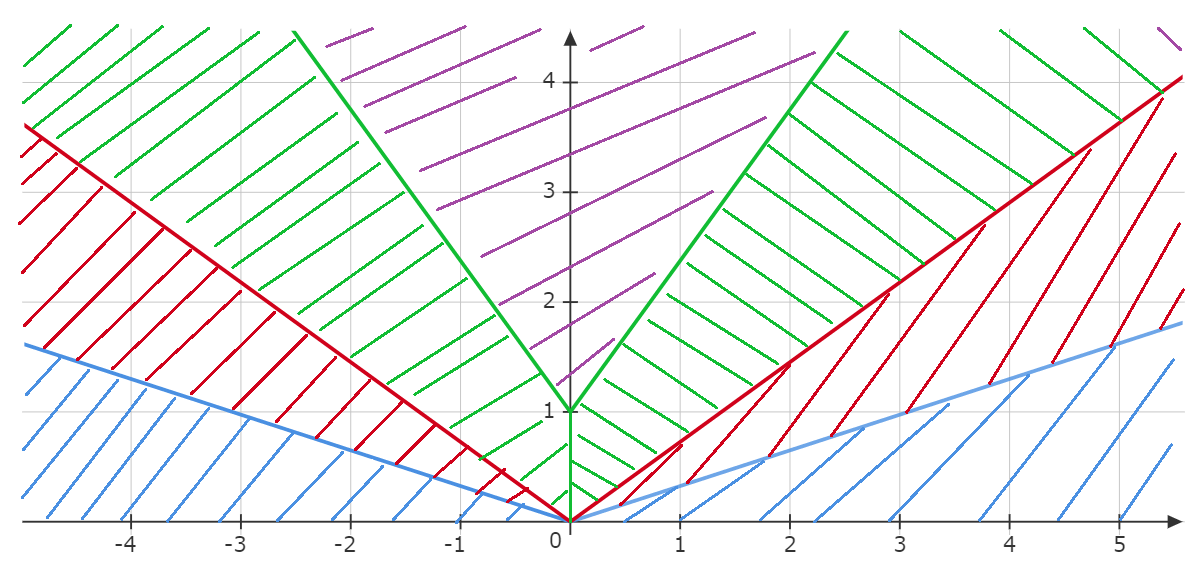
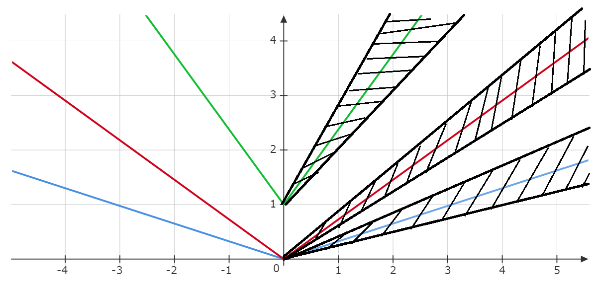
Figure 5: This figure shows the support of the different automorphisms present in the decomposition of an SQ₁-automorphism acting on the upper half plane.

As a remark, notice that this definition is not exactly identical to de definition given in [10] due to the translation operators.

Definition J.2.

Take $\alpha\in\textrm{Aut}\mathopen{}\mathclose{{}\left(\mathcal{A}}\right)$. We say that $\alpha\in\textrm{HAut}_{1}(\mathcal{A})$ if and only if for any $0<\theta<\pi/2$ there exists an $a\in\mathcal{A}$ and some $\alpha_{\sigma}\in\textrm{Aut}\mathopen{}\mathclose{{}\left(\mathcal{A}_{C_{\theta}}\cap\mathcal{A}_{\sigma}}\right)$ for each $\sigma\in\{L,R\}$ such that

$$\alpha=\textrm{Ad}\mathopen{}\mathclose{{}\left(a}\right)\circ\alpha_{L}\otimes\alpha_{R}.$$ (J.3)

We will need one additional class of automorphisms:

Definition J.3.

Take $\alpha\in\textrm{Aut}\mathopen{}\mathclose{{}\left(\mathcal{A}}\right)$. We say that $\alpha\in\textrm{VAut}_{1}(\mathcal{A})$ if and only if there exists some $a\in\mathcal{A}$, $\alpha_{U}\in\textrm{Aut}\mathopen{}\mathclose{{}\left(\tau(\mathcal{A}_{C_{\theta}^{c}}\cap\mathcal{A}_{U})}\right)$ and an $\alpha_{D}\in\textrm{Aut}\mathopen{}\mathclose{{}\left(\tau^{-1}(\mathcal{A}_{C_{\theta}^{c}}\cap\mathcal{A}_{D})}\right)$ such that

$$\alpha=\textrm{Ad}\mathopen{}\mathclose{{}\left(a}\right)\circ\alpha_{U}\otimes\alpha_{D}.$$ (J.4)

If furthermore $\alpha_{U}\circ\beta_{g}^{U}=\beta_{g}^{U}\circ\alpha_{U}$ we say that $\alpha\in\textrm{GVAut}_{1}(\mathcal{A})$.

Now we will state some properties of locally generated automorphisms:

Lemma J.4.

Take $H$ an interaction such that there exists a $0<\phi<1$ satisfying that $\norm{H}_{f_{\phi}}\leq 1$. The following statements now hold (for any $s,t\in\mathbb{R}$):

1. $\gamma^{H}_{s;t}\circ\gamma^{H_{D}}_{t;s}\otimes\gamma^{H_{U}}_{t;s}\in\textrm{HAut}_{1}(\mathcal{A})$.

2. $\gamma^{H}_{s;t}\circ\gamma^{H_{L}}_{t;s}\otimes\gamma^{H_{R}}_{t;s}\in\textrm{VAut}_{1}(\mathcal{A})$. If additionally $H$ is a $G$-invariant interaction we even have $\gamma^{H}_{s;t}\circ\gamma^{H_{L}}_{t;s}\otimes\gamma^{H_{R}}_{t;s}\in\textrm{GVQAut}_{1}(\mathcal{A})$.

3. $\gamma^{H_{U}}_{s;t}\otimes\gamma^{H_{D}}_{s;t}\in\textrm{SQAut}_{1}(\mathcal{A})$. If additionally $H$ is a $G$-invariant interaction we even have $\gamma^{H_{U}}_{s;t}\otimes\gamma^{H_{D}}_{s;t}\in\textrm{GSQAut}_{1}(\mathcal{A})$.

4. If $H$ is $G$-invariant then $\gamma^{H}_{t;s}\circ\beta_{g}^{U}\circ\gamma^{H}_{s;t}\circ(\beta_{g}^{U})^{-1}\in\textrm{HAut}_{1}(\mathcal{A})$.

5. $\gamma^{H}_{t;s}\in\textrm{SQAut}_{1}(\mathcal{A})$.

Proof.

Part 1 is done in Proposition 5.5 in [10] and part 4 follows trivially from Part 1. Except for the translation operators in my definition of the $\textrm{SQAut}(\mathcal{A})$, part 3 follows from Theorem 5.2 in [10]. To show part 3 we therefore have to show that Theorem 5.2 in [10] still holds if we replace $\mathcal{C}_{0}$ and $\mathcal{C}_{1}$ in the proof by

$$\mathcal{C}_{0} \vcentcolon=\mathopen{}\mathclose{{}\left\{C_{[0,\theta_{1}],\sigma},C_{]\theta_{1},\theta_{2}],\sigma,\rho},C_{]\theta_{2},\theta_{3}],\sigma,\rho}\cup\tau^{\rho}(C_{]\theta_{2},\theta_{3}],\sigma,\rho}),\tau^{\rho}(C_{]\theta_{3},\pi/2],\rho})|\sigma=\{L,R\},\rho=\{U,D\}}\right\}$$ (J.5)

$$\mathcal{C}_{1} \vcentcolon=\{C_{[\theta_{0.8},\theta_{1.2}]\cap\sigma\cap\tau},C_{[\theta_{1.8},\theta_{2.2}]\cap\sigma\cap\tau},\tau^{\rho}(C_{[\theta_{2.8},\theta_{3.2}]\cap\sigma\cap\rho})|\sigma=\{L,R\},\rho=\{U,D\}\}.$$ (J.6)

Take the $\Psi$ from this proof to be our $H$, take $\Psi^{(0)}$ to be $\sum_{C\in\mathcal{C}_{0}}H_{C}$ (with our new definition of $\mathcal{C}_{0}$) and take $\Psi^{(1)}\vcentcolon=\Psi-\Psi^{(0)}$. Now define $\Xi^{(s)}(Z,t)$ through

$$\Xi^{(s)}(Z,t)\vcentcolon=\sum_{m=0}^{\infty}\sum_{\begin{subarray}{c}X\subset Z,\\ X(m)=Z\end{subarray}}\Delta_{X(m)}(\gamma^{\Psi}_{s;t}(\Psi^{(1)}(X;t)))$$ (J.7)

with these new definitions of $\Psi^{(0)}$ and $\Psi^{(1)}$. We now want so show that for every $t$,

$$\sum_{Z\subset\mathbb{Z}^{2}}\mathopen{}\mathclose{{}\left(\Xi^{(s)}(Z,t)-\sum_{C\in\mathcal{C}_{1}}\mathbbm{1}_{Z\subset C}\Xi^{(s)}(Z,t)}\right)$$ (J.8)

is bounded. Following the arguments in equation (5.22) to (5.24) in [10] we still get that

$$\sum_{\begin{subarray}{c}Z\subset\mathbb{Z}^{2},\\ \nexists C\in\mathcal{C}_{1}:Z\subset C\end{subarray}}\sup_{t\in[0,1]}\norm{\Xi^{(1)}(Z,t)}\leq\frac{8}{C_{F}}(e^{2I_{F}(\Psi)}-1)\sum_{\begin{subarray}{c}C_{1},C_{2}\in\mathcal{C}_{0},\\ C_{1}\neq C_{2}\end{subarray}}M(C_{1},C_{2})$$ (J.9)

where

$$M(C_{1},C_{2})\vcentcolon=\sum_{m\geq 0}\sum_{\begin{subarray}{c}X:\\ \forall C\in\mathcal{C}_{1},X\cap((C^{c})(m))\neq\emptyset,\\ X\cap C_{1}\neq\emptyset,X\cap C_{2}\neq\emptyset\end{subarray}}\mathopen{}\mathclose{{}\left(\sup_{t\in[0,1]}(\norm{\Psi^{(1)}(X;t)})\absolutevalue{X}G_{F}(m)}\right)$$ (J.10)

is now defined using the new $\mathcal{C}_{1}$. To bound these $M(C_{1},C_{2})$ we will (just like in [10]) differentiate between two cases. That is, the case where $C_{1}$ and $C_{2}$ are adjacent and the case where they are not. We begin with the latter. In this case we still have in complete analogy with the proof in [10] that

$$M(C_{1},C_{2})\leq b_{0}(C_{1},C_{2}) \vcentcolon=\sum_{m\geq 0}\sum_{\begin{subarray}{c}X:X\cap C_{1}\neq\emptyset,\\ X\cap C_{2}\neq\emptyset\end{subarray}}\mathopen{}\mathclose{{}\left(\sup_{t\in[0,1]}(\norm{\Psi^{(1)}(X;t)})\absolutevalue{X}G_{F}(m)}\right)$$ (J.11)

$$\leq\norm{\Psi_{1}}_{F}\sum_{\begin{subarray}{c}x\in C_{1}\\ y\in C_{2}\end{subarray}}F(d(x,y))\sum_{m=0}^{\infty}G_{F}(m)<\infty.$$ (J.12)

What is now left to show is the case where $C_{1}$ and $C_{2}$ are adjacent. Take $\tilde{C}\in\mathcal{C}_{1}$ such that $C_{1}\cap\tilde{C}\neq\emptyset$ and $C_{2}\cap\tilde{C}\neq\emptyset$. Take $L_{1}=\partial\tilde{C}/C_{2}$ and $L_{2}=\partial\tilde{C}/C_{1}$. By following the same reasoning that led to equation (5.36) in [10] we get that

$$M(C_{1},C_{2})\leq b_{0}(C_{1},C_{2}/\tilde{C})+b_{0}(C_{1}/\tilde{C},C_{2})+b_{0}(\tilde{C}\cap C_{2},(C_{1}\cup C_{2})^{c})+b_{1}(C_{1}\cap\tilde{C},C_{2}\cap\tilde{C},L_{1},L_{2})$$ (J.13)

where

$$b_{1}(C_{1}\cap\tilde{C},C_{2}\cap\tilde{C},L_{1},L_{2}) \vcentcolon=\sum_{m=0}^{\infty}\sum_{\begin{subarray}{c}X\subset\tilde{C}:\\ X\cap C_{1}\cap\tilde{C}\neq\emptyset\\ X\cap C_{2}\cap\tilde{C}\neq\emptyset\\ X\cap(\tilde{C}^{c}(m))\neq\emptyset\end{subarray}}\sup_{t\in[0,1]}\norm{\Psi(X;t)}\absolutevalue{X}G_{F}(m)$$ (J.14)

$$\leq\norm{\Psi_{1}}_{F}\sum_{m=0}^{\infty}G_{F}(m)\mathopen{}\mathclose{{}\left(\sum_{\begin{subarray}{c}x\in C_{2}\cap\tilde{C},\\ y\in L_{1}(m)\end{subarray}}+\sum_{\begin{subarray}{c}x\in C_{1}\cap\tilde{C},\\ y\in L_{2}(m)\end{subarray}}}\right)F(d(x,y))<\infty.$$ (J.15)

Since the remainder of the proof can remain unchanged from [10], this concludes the proof of item 3. The proof of item 5 just follows from the fact that for any $\alpha_{1}\in\textrm{SQAut}(\mathcal{A})$ and for any $\alpha_{2}\in\textrm{HAut}(\mathcal{A})$ we have that $\alpha_{2}\circ\alpha_{1}\in\textrm{SQAut}(\mathcal{A})$. We now only need to comment on item 2. We must show that

$$(\gamma^{H}_{s;t}\circ\gamma^{H_{L}}_{t;s}\otimes\gamma^{H_{R}}_{t;s})^{-1}=\gamma^{H_{L}}_{s;t}\otimes\gamma^{H_{R}}_{s;t}\circ\gamma^{H}_{t;s}\in\textrm{GVAut}(\mathcal{A}).$$ (J.16)

The proof of this starts analogously to the proof of item 1 and 3. We take $\Psi=H$, $\Psi^{(0)}=H_{\tau(C_{\theta}^{c}\cap U)}+H_{\tau^{-1}(C_{\theta}^{c}\cap D)}$ and $\Psi^{(1)}=\Psi-\Psi^{(0)}$. Define $\Xi^{(s)}(Z;t)$ again through equation (J.7). In analogy to what was done in equation (5.54) in [10] we obtain

$$\sum_{\begin{subarray}{c}Z:Z\nsubseteq\tau(C_{\theta}^{c}\cap U)\\ \text{and }Z\nsubseteq\tau^{-1}(C_{\theta}^{c}\cap D)\end{subarray}}\sup_{t\in[0,1]}\norm{\Xi^{(1)}(Z,t)}\leq\frac{8}{C_{F}}(e^{2I_{F}(\Psi)}-1)\sum_{m=0}^{\infty}\sum_{\begin{subarray}{c}X:X(m)\nsubseteq\tau(C_{\theta}^{c}\cap U)\\ \text{and }X(m)\nsubseteq\tau^{-1}(C_{\theta}^{c}\cap D)\end{subarray}}\sup_{t\in[0,1]}\norm{\Psi^{(1)}(X;t)}\absolutevalue{X}G_{F}(m).$$ (J.17)

If $X$ in the last line has a non-zero contribution, then at least one of the following occurs:

1. $X\cap(W(C_{\theta})\cap L)\neq\emptyset$ and $X\cap R\neq\emptyset$.

2. $X\cap(W(C_{\theta})\cap R)\neq\emptyset$ and $X\cap L\neq\emptyset$.

3. $X\subset W(C_{\theta})^{c}$ and

   1. $X\subset U,X\subset D$, or

   2. $X\subset U,X\subset L,X\subset R$ and $X(m)\cap(\tau^{-1}(C_{\theta}^{c}\cap D))^{c}\neq\emptyset$, or

   3. $X\subset D,X\subset L,X\subset R$ and $X(m)\cap(\tau(C_{\theta}^{c}\cap U))^{c}\neq\emptyset$.

This shows that we have a bound

$$\sum_{\begin{subarray}{c}Z:Z\nsubseteq\tau(C_{\theta}^{c}\cap U)\\ \text{and }Z\nsubseteq\tau^{-1}(C_{\theta}^{c}\cap D)\end{subarray}}\sup_{t\in[0,1]}\norm{\Xi^{(1)}(Z,t)}$$ (J.18)

$$\leq\frac{8}{C_{F}}(e^{2I_{F}(\Psi)}-1)(b_{0}(W(C_{\theta})\cap L,R)+b_{0}(L,W(C_{\theta})\cap R)+b_{0}(W(C_{\theta})^{c}\cap U,W(C_{\theta})^{c}\cap D)$$

$$\qquad+b_{1}(W(C_{\theta})^{c}\cap U\cap L,W(C_{\theta})^{c}\cap U\cap L,L\cap\partial(W(C_{\theta})^{c}\cap U),R\cap\partial(W(C_{\theta})^{c}\cap U))$$

$$\qquad b_{1}(W(C_{\theta})^{c}\cap D\cap L,W(C_{\theta})^{c}\cap D\cap R,L\cap\partial(W(C_{\theta})^{c}\cap D),R\cap\partial(W(C_{\theta})^{c}\cap D)))<\infty.$$ (J.19)

This concludes the proof. ∎

This implies certain things for our locally generated automorphisms. From these four statements we can prove the following results:

Lemma J.5.

Take $H$ an interaction such that there exists a $0<\phi<1$ satisfying that $\norm{H}_{f_{\phi}}\leq 1$. Take $\theta_{1}$ and $\theta_{2}$ such that $0<\theta_{1}<\theta_{2}<\pi/2$ then for all $\Theta\in\textrm{Aut}\mathopen{}\mathclose{{}\left(\mathcal{A}_{W(C_{\theta_{2}})^{c}}}\right)$ and $s,t\in\mathbb{R}$ there exists an $a_{1}\in\mathcal{U}(\mathcal{A})$ and a $\tilde{\Theta}\in\textrm{Aut}\mathopen{}\mathclose{{}\left(\mathcal{A}_{W(C_{\theta_{1}})^{c}}}\right)$ such that

$$\gamma^{H}_{t;s}\circ\Theta\circ\gamma^{H}_{s;t}=\textrm{Ad}\mathopen{}\mathclose{{}\left(a_{1}}\right)\circ\tilde{\Theta}.$$ (J.20)

Proof.

We have that

$$\gamma^{H}_{t;s}\circ\Theta\circ\gamma^{H}_{s;t}=\gamma^{H_{D}}_{t;s}\otimes\gamma^{H_{U}}_{t;s}\circ\gamma^{H_{D}}_{s;t}\otimes\gamma^{H_{U}}_{s;t}\circ\gamma^{H}_{t;s}\circ\Theta\circ\gamma^{H}_{s;t}\circ\gamma^{H_{D}}_{t;s}\otimes\gamma^{H_{U}}_{t;s}\circ\gamma^{H_{D}}_{s;t}\otimes\gamma^{H_{U}}_{s;t}.$$ (J.21)

Using that $\gamma^{H}_{s;t}\circ\gamma^{H_{D}}_{t;s}\otimes\gamma^{H_{U}}_{t;s}\in\textrm{HAut}_{1}(\mathcal{A})$ we get that there exists some $a\in\mathcal{A}$ and $\eta\in\textrm{Aut}\mathopen{}\mathclose{{}\left(\mathcal{A}_{C_{\theta}}}\right)$ such that

$$\gamma^{H}_{t;s}\circ\Theta\circ\gamma^{H}_{s;t} =\textrm{Ad}\mathopen{}\mathclose{{}\left(a}\right)\circ\gamma^{H_{D}}_{t;s}\otimes\gamma^{H_{U}}_{t;s}\circ\eta_{s;t}^{-1}\circ\Theta\circ\eta_{s;t}\circ\gamma^{H_{D}}_{s;t}\otimes\gamma^{H_{U}}_{s;t}$$ (J.22)

$$=\textrm{Ad}\mathopen{}\mathclose{{}\left(a}\right)\circ\gamma^{H_{D}}_{t;s}\otimes\gamma^{H_{U}}_{t;s}\circ\Theta\circ\gamma^{H_{D}}_{s;t}\otimes\gamma^{H_{U}}_{s;t}.$$ (J.23)

Since by J.4 part 3 $\gamma^{H_{D}}_{s;t}\otimes\gamma^{H_{U}}_{s;t}\in\textrm{GSQAut}_{1}(\mathcal{A})$ the result follows. ∎

Lemma J.6.

Take $H$ an interaction such that there exists a $0<\phi<1$ satisfying that $\norm{H}_{f_{\phi}}\leq 1$. Take $\theta_{1}$ and $\theta_{2}$ such that $0<\theta_{1}<\theta_{2}<\pi/2$. Then for all $\eta_{g}^{\sigma}\in\textrm{Aut}\mathopen{}\mathclose{{}\left(\mathcal{A}_{C_{\theta_{1}}}\cap\mathcal{A}_{\sigma}}\right)$ (where $\sigma\in\{L,R\}$ and $g\in G$) and $s,t\in\mathbb{R}$ there exist $a_{2},\in\mathcal{U}(\mathcal{A}),a_{3,\sigma}\in\mathcal{U}(\mathcal{A}_{\sigma})$ and some $\tilde{\eta}_{\sigma}^{g}\in\textrm{Aut}\mathopen{}\mathclose{{}\left(\mathcal{A}_{C_{\theta_{2}}}\cap\mathcal{A}_{\sigma}}\right)$ such that

$$\gamma^{H}_{t;s}\circ\eta_{g}^{L}\otimes\eta_{g}^{R}\circ\gamma^{H}_{s;t} =\textrm{Ad}\mathopen{}\mathclose{{}\left(a_{2}}\right)\circ(\tilde{\eta}_{g}^{L}\otimes\tilde{\eta}_{g}^{R})$$ (J.24)

$$\gamma^{H_{\sigma}}_{t;s}\circ\eta_{g}^{\sigma}\circ\gamma^{H_{\sigma}}_{s;t} =\textrm{Ad}\mathopen{}\mathclose{{}\left(a_{3,\sigma}}\right)\circ\tilde{\eta}_{g}^{\sigma}.$$ (J.25)

Proof.

In this proof, take ${H_{\text{split}}}=H_{L}+H_{R}$. First we show that equation (J.25) implies equation (J.24). This is because using equation (J.24) we get that

$$\gamma^{H}_{t;s}\circ\eta_{g}\circ\gamma^{H}_{s;t} =\gamma^{H}_{t;s}\circ\gamma^{{H_{\text{split}}}}_{s;t}\circ\gamma^{{H_{\text{split}}}}_{t;s}\circ\eta_{g}\circ\gamma^{{H_{\text{split}}}}_{s;t}\circ\gamma^{{H_{\text{split}}}}_{t;s}\circ\gamma^{H}_{s;t}$$ (J.26)

$$=\gamma^{H}_{t;s}\circ\gamma^{{H_{\text{split}}}}_{s;t}\circ\textrm{Ad}\mathopen{}\mathclose{{}\left(a_{3,L}\otimes a_{3,R}}\right)\circ\tilde{\eta}_{g}\circ\gamma^{{H_{\text{split}}}}_{t;s}\circ\gamma^{H}_{s;t}.$$ (J.27)

If one now uses the fact that $\gamma^{H}_{t;s}\circ\gamma^{{H_{\text{split}}}}_{s;t}\in\textrm{GVAut}_{1}(\mathcal{A})$ (see lemma J.4 item 2) the implication follows. To finish the proof we now only have to use the fact that the $\gamma^{H_{\sigma}}_{0;1}$ are in $\textrm{SQAut}_{1}(\mathcal{A}_{\sigma})$. ∎

Additionally when we add the group action, we get:

Lemma J.7.

Take $H$ a $G$-invariant interaction such that there exists a $0<\phi<1$ satisfying that $\norm{H}_{f_{\phi}}\leq 1$. Take $\theta_{1}$ and $\theta_{2}$ such that $0<\theta_{1}<\theta_{2}<\pi/2$. Then for all $\eta_{g}^{\sigma}\in\textrm{Aut}\mathopen{}\mathclose{{}\left(\mathcal{A}_{C_{\theta_{1}}}\cap\mathcal{A}_{\sigma}}\right)$ (where $\sigma\in\{L,R\}$ and $g\in G$) and $s,t\in\mathbb{R}$ there exist $a_{2},\in\mathcal{U}(\mathcal{A}),a_{3,\sigma}\in\mathcal{U}(\mathcal{A}_{\sigma})$ and some $\tilde{\eta}_{\sigma}^{g}\in\textrm{Aut}\mathopen{}\mathclose{{}\left(\mathcal{A}_{C_{\theta_{2}}}\cap\mathcal{A}_{\sigma}}\right)$ such that

$$\gamma^{H}_{t;s}\circ\eta_{g}^{L}\otimes\eta_{g}^{R}\circ\beta_{g}^{U}\circ\gamma^{H}_{s;t} =\textrm{Ad}\mathopen{}\mathclose{{}\left(a_{2}}\right)\circ(\tilde{\eta}_{g}^{L}\otimes\tilde{\eta}_{g}^{R})\circ\beta_{g}^{U}$$ (J.28)

$$\gamma^{H_{\sigma}}_{t;s}\circ\eta_{g}^{\sigma}\circ\beta_{g}^{\sigma U}\circ\gamma^{H_{\sigma}}_{s;t} =\textrm{Ad}\mathopen{}\mathclose{{}\left(a_{3,\sigma}}\right)\circ\tilde{\eta}_{g}^{\sigma}\circ\beta_{g}^{\sigma U}.$$ (J.29)

Proof.

In this proof, take again ${H_{\text{split}}}=H_{L}+H_{R}$. First we show that equation (J.29) implies equation (J.28). This is because using (the inverse of) equation (J.28) we get that

$$\gamma^{H}_{t;s}\circ\eta_{g}\circ\beta_{g}^{U}\circ\gamma^{H}_{s;t}\circ\beta_{g^{-1}}^{U}\circ(\tilde{\eta}_{g})^{-1}$$ (J.30)

$$=(\text{Inner})\circ\gamma^{H}_{t;s}\circ\eta_{g}\circ\beta_{g}^{U}\circ\gamma^{H}_{s;t}\circ\gamma^{H_{\text{split}}}_{t;s}\circ\beta_{g^{-1}}^{U}\circ(\eta_{g})^{-1}\circ\gamma^{H_{\text{split}}}_{s;t}\circ\underline{\gamma^{H}_{t;s}\circ\gamma^{H}_{s;t}}.$$ (J.31)

Now using the fact that by lemma J.4 item 2, $\gamma^{H}_{s;t}\circ\gamma^{H_{\text{split}}}_{t;s}\in\textrm{GVAut}_{1}(\mathcal{A})$ this gives us

$$=(\text{Inner})\circ\text{\sout{$\gamma^{H}_{t;s}\circ\eta_{g}\circ\beta_{g}^{U}\circ\beta_{g^{-1}}^{U}\circ(\eta_{g})^{-1}\circ\gamma^{H}_{s;t}$}}.$$ (J.32)

By taking $a_{2}$ such that $\textrm{Ad}\mathopen{}\mathclose{{}\left(a_{2}}\right)$ is this inner automorphism, we can conclude the proof that equation (J.29) implies equation (J.28). Now we only have to prove equation (J.29). To finish the proof we now only have to use the fact that the $\gamma^{H_{\sigma}}_{0;1}$ are in $\textrm{GSQAut}_{1}(\mathcal{A}_{\sigma})$. ∎

J.2 The two translation symmetries

This section will define the classes of automorphisms required in the assumptions and proofs about the $H^{1}$-valued translation index. In analogy with section 2.1 from [10] we will define some classes of automorphisms (see figure 6):

Definition J.8.

Take $\alpha\in\textrm{Aut}\mathopen{}\mathclose{{}\left(\mathcal{A}}\right)$. We say that $\alpha\in\textrm{SQAut}_{2}(\mathcal{A})$ if and only if for any $0<\theta_{0.8}<\theta_{1}<\theta_{1.2}<\theta_{1.8}<\theta_{2}<\theta_{2.2}<\theta_{2.8}<\theta_{3}<\theta_{3.2}<\pi/2$ there exist $a\in\mathcal{A}$, $\alpha_{[0,\theta_{1}],\sigma}\in\textrm{Aut}\mathopen{}\mathclose{{}\left(\mathcal{A}_{\nu^{\sigma}(C_{[0,\theta_{1}]}\cap\sigma)}}\right),\>\alpha_{]\theta_{1},\theta_{2}],\sigma,\rho}\in\textrm{Aut}\mathopen{}\mathclose{{}\left(\mathcal{A}_{\nu^{\sigma}(C_{]\theta_{1},\theta_{2}]}\cap\rho\cap\sigma)}}\right),\>\alpha_{]\theta_{2},\theta_{3}],\sigma,\rho}\in\textrm{Aut}\mathopen{}\mathclose{{}\left(\mathcal{A}_{(W(C_{[0,\theta_{3}]})/\nu^{\sigma}(C_{[0,\theta_{2}]}\cap\sigma))\cap\rho\cap\sigma)}}\right),\\ \alpha_{]\theta_{3},\pi/2],\rho}\in\textrm{Aut}\mathopen{}\mathclose{{}\left(\mathcal{A}_{\tau^{\rho}(C_{[\theta_{3},\pi/2]}\cap\rho)}}\right),\>\alpha_{]\theta_{0.8},\theta_{1.2}],\sigma,\rho}\in\textrm{Aut}\mathopen{}\mathclose{{}\left(\mathcal{A}_{\nu^{\sigma}(C_{]\theta_{0.8},\theta_{1.2}]}\cap\rho\cap\sigma)}}\right),\\ \alpha_{]\theta_{1.8},\theta_{2.2}],\sigma,\rho}\in\textrm{Aut}\mathopen{}\mathclose{{}\left(\mathcal{A}_{\nu^{\sigma}(C_{]\theta_{1.8},\theta_{2.2}]}\cap\rho\cap\sigma)}}\right)$ and $\alpha_{]\theta_{2.8},\theta_{3.2}],\sigma,\rho}\in\textrm{Aut}\mathopen{}\mathclose{{}\left(\mathcal{A}_{\tau^{\rho}(C_{]\theta_{2.8},\theta_{3.2}]}\cap\rho\cap\sigma)}}\right)$ for any $\rho\in\{U,D\}$ and $\sigma\in\{L,R\}$ (here $\tau^{U}=\tau$, $\tau^{D}=\tau^{-1}$, $\nu^{R}=\nu$ and $\nu^{L}=\nu^{-1}$) such that

$$\alpha=\textrm{Ad}\mathopen{}\mathclose{{}\left(a}\right)\circ\bigotimes_{\sigma}\alpha_{[0,\theta_{1}],\sigma}\circ\bigotimes_{\sigma,\rho}\alpha_{]\theta_{1},\theta_{2}],\sigma,\rho}\circ\bigotimes_{\rho}\alpha_{[\theta_{3},\pi/2]}\circ\bigotimes_{\rho,\sigma}\mathopen{}\mathclose{{}\left(\alpha_{]\theta_{0.8},\theta_{1.2}],\rho,\sigma}\otimes\alpha_{]\theta_{1.8},\theta_{2.2}],\rho,\sigma}\otimes\alpha_{]\theta_{2.8},\theta_{3.2}],\rho,\sigma}}\right).$$ (J.33)

If additionally everything (except $a$) commutes with $\beta_{g}^{U}$ we say that $\alpha\in\textrm{GSQAut}_{2}(\mathcal{A})$.

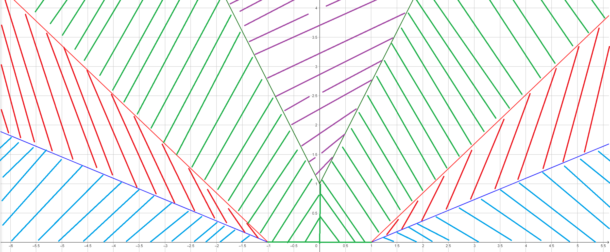
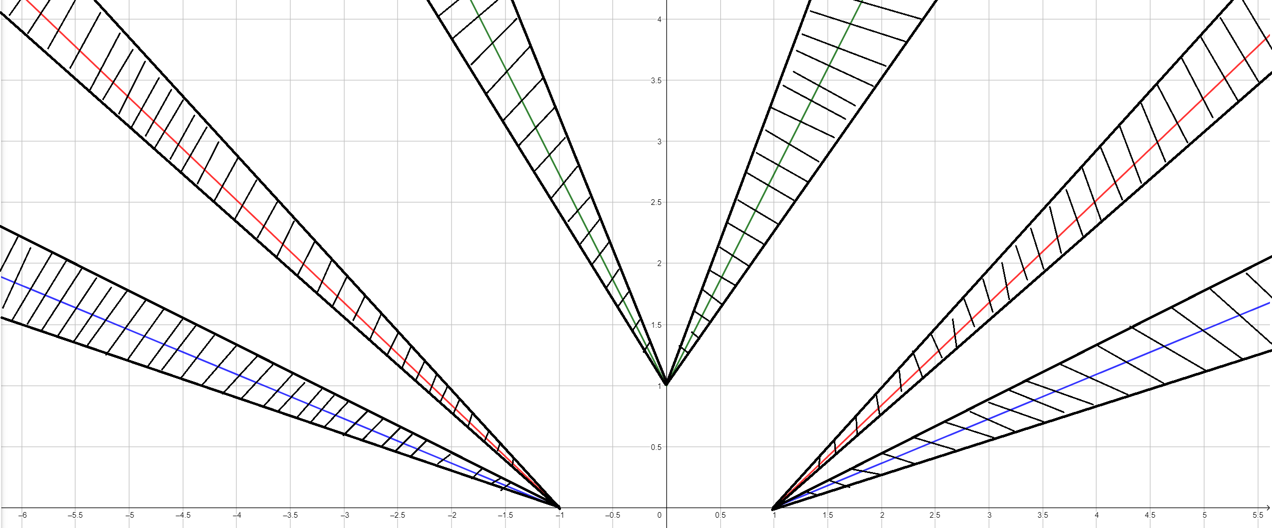
Figure 6: This figure shows the support of the different automorphisms present in the decomposition of an SQ₂-automorphism acting on the upper half plane.

We now have to define a different horizontal automorphism:

Definition J.9.

Take $\alpha\in\textrm{Aut}\mathopen{}\mathclose{{}\left(\mathcal{A}}\right)$. We say that $\alpha\in\textrm{HAut}_{2}(\mathcal{A})$ if and only if for any $0<\theta<\pi/2$ there exists an $a\in\mathcal{A}$ and some $\alpha_{\sigma}\in\textrm{Aut}\mathopen{}\mathclose{{}\left(\mathcal{A}_{\nu^{\sigma}(C_{\theta}\cap\sigma)}}\right)$ for each $\sigma\in\{L,R\}$ such that

$$\alpha=\textrm{Ad}\mathopen{}\mathclose{{}\left(a}\right)\circ\alpha_{L}\otimes\alpha_{R}.$$ (J.34)

The main reason why we introduce this new class of automorphisms is that if $\alpha\in\textrm{HAut}_{2}(\mathcal{A})$ we automatically have that the translations of $\alpha$ in the horizontal directions, $\nu^{-1}\circ\alpha\circ\nu$ and $\nu\circ\alpha\circ\nu^{-1}$ are elements of $\textrm{HAut}_{1}(\mathcal{A})$. We will let the definition of vertical automorphism stay the same, namely $\textrm{VAut}_{2}(\mathcal{A})=\textrm{VAut}_{1}(\mathcal{A})$ and $\textrm{GVAut}_{2}(\mathcal{A})=\textrm{GVAut}_{1}(\mathcal{A})$.

Lemma J.10.

Lemma J.4 will still be true when we exchange all the ₁’s for ₂’s.

Proof.

Completely equivalent to the proof of J.4. ∎

Lemma J.11.

Take $\theta_{1}$ and $\theta_{2}$ such that $0<\theta_{1}<\theta_{2}<\pi/2$. Then for all $\eta_{g}^{\sigma}\in\textrm{Aut}\mathopen{}\mathclose{{}\left(\mathcal{A}_{\nu^{\sigma}(C_{\theta_{1}}\cap\sigma)}}\right)$ (where $\sigma\in\{L,R\}$ and $g\in G$), there exist $a_{2},\in\mathcal{U}(\mathcal{A}),a_{3,\sigma}\in\mathcal{U}(\mathcal{A}_{\nu^{\sigma}(\sigma)})$ and some $\tilde{\eta}_{\sigma}^{g}\in\textrm{Aut}\mathopen{}\mathclose{{}\left(\mathcal{A}_{\nu^{\sigma}(C_{\theta_{2}}\cap\sigma)}}\right)$ such that

$$\gamma^{H}_{1;0}\circ\eta_{g}^{L}\otimes\eta_{g}^{R}\circ\gamma^{H}_{0;1} =\textrm{Ad}\mathopen{}\mathclose{{}\left(a_{2}}\right)\circ(\tilde{\eta}_{g}^{L}\otimes\tilde{\eta}_{g}^{R})$$ (J.35)

$$\gamma^{H_{\nu^{\sigma}(\sigma)}}_{1;0}\eta_{g}^{\sigma}\gamma^{H_{\nu^{\sigma}(\sigma)}}_{0;1} =\textrm{Ad}\mathopen{}\mathclose{{}\left(a_{3,\sigma}}\right)\circ\tilde{\eta}_{g}^{\sigma}.$$ (J.36)

Proof.

Analogous to the proof of J.6. ∎

Additionally when we add the group action, we get:

Lemma J.12.

Take $H$ a $G$-invariant interaction such that there exists a $0<\phi<1$ satisfying that $\norm{H}_{f_{\phi}}\leq 1$. Take $\theta_{1}$ and $\theta_{2}$ such that $0<\theta_{1}<\theta_{2}<\pi/2$. Then for all $\eta_{g}^{\sigma}\in\textrm{Aut}\mathopen{}\mathclose{{}\left(\mathcal{A}_{C_{\theta_{1}}}\cap\mathcal{A}_{\sigma}}\right)$ (where $\sigma\in\{L,R\}$ and $g\in G$), there exist $a_{2},\in\mathcal{U}(\mathcal{A}),a_{3,\sigma}\in\mathcal{U}(\mathcal{A}_{\sigma})$ and some $\tilde{\eta}_{\sigma}^{g}\in\textrm{Aut}\mathopen{}\mathclose{{}\left(\mathcal{A}_{\nu^{\sigma}(C_{\theta_{2}}\cap\sigma)}}\right)$ such that

$$\gamma^{H}_{1;0}\circ\eta_{g}^{L}\otimes\eta_{g}^{R}\circ\beta_{g}^{U}\circ\gamma^{H}_{0;1} =\textrm{Ad}\mathopen{}\mathclose{{}\left(a_{2}}\right)\circ(\tilde{\eta}_{g}^{L}\otimes\tilde{\eta}_{g}^{R})\circ\beta_{g}^{U}$$ (J.37)

$$\gamma^{H_{\sigma}}_{1;0}\circ\eta_{g}^{\sigma}\circ\beta_{g}^{\sigma U}\circ\gamma^{H_{\sigma}}_{0;1} =\textrm{Ad}\mathopen{}\mathclose{{}\left(a_{3,\sigma}}\right)\circ\tilde{\eta}_{g}^{\sigma}\circ\beta_{g}^{\sigma U}.$$ (J.38)

Proof.

Analogous to the proof of J.7. ∎

In what follows, let ${\tilde{H}_{\text{split}}}\vcentcolon=H_{\nu^{-1}(L)}+H_{\nu(R)}$. We will need the following lemma:

Lemma J.13.

There exist maps

$$A_{L} :[0,1]\rightarrow\mathcal{U}(\mathcal{A}_{L}):\lambda\mapsto A_{L}(\lambda) A_{R} :[0,1]\rightarrow\mathcal{U}(\mathcal{A}_{R}):\lambda\mapsto A_{R}(\lambda)$$ (J.39)

both continuous in norm topology and

$$\Phi^{\mu\nu}:[0,1]\rightarrow\textrm{Aut}\mathopen{}\mathclose{{}\left(\mathcal{A}_{W(C_{\theta})^{c}\cap\mu\cap\nu}}\right):\lambda\mapsto\Phi^{\mu\nu}(\lambda)$$ (J.40)

where $\mu\in\{U,D\}$ and $\nu\in\{L,\nu(R)\}$, all four continuous in strong topology, satisfying that

$$\nu\circ\gamma^{{\tilde{H}_{\text{split}}}}_{0;\lambda}\circ\nu^{-1}\circ\gamma^{{\tilde{H}_{\text{split}}}}_{\lambda;0} =\gamma^{H_{L}}_{0;\lambda}\otimes\gamma^{H_{\nu\circ\nu(R)}}_{0;\lambda}\circ\gamma^{{\tilde{H}_{\text{split}}}}_{\lambda;0}$$ (J.41)

$$=\textrm{Ad}\mathopen{}\mathclose{{}\left(A_{L}(\lambda)}\right)\otimes\textrm{Ad}\mathopen{}\mathclose{{}\left(A_{R}(\lambda)}\right)\circ\bigotimes_{\begin{subarray}{c}\mu\in\{U,D\},\\ \nu\in\{L,\nu(R)\}\end{subarray}}\Phi^{\mu\nu}(\lambda)$$ (J.42)

and that $\Phi^{\mu\nu}\circ\beta_{g}=\beta_{g}\circ\Phi^{\mu\nu}$.

Proof.

The proof of this is very similar to all the other proofs in this section. We will go over the highlights. We want to define an $A_{L}(\lambda)$ and a $\Phi^{U,L}\otimes\Phi^{D,L}$ satisfying

$$\textrm{Ad}\mathopen{}\mathclose{{}\left(A_{L}(\lambda)}\right)\circ\Phi^{U,L}\otimes\Phi^{D,L}(\lambda)=\gamma^{H_{L}}_{0;\lambda}\circ\gamma^{H_{\nu^{-1}(L)}}_{\lambda;0}$$ (J.43)

and similarly for the right side. We will only work out this side as the other calculation is analogous. We do this in two steps. First we find an interaction $\Xi$ satisfying

$$\gamma^{\Xi}_{0;\lambda}=\gamma^{H_{L}}_{0;\lambda}\circ\gamma^{H_{\nu^{-1}(L)}}_{\lambda;0}.$$ (J.44)

We can do this by taking the usual

$$\Xi(Z,t)\vcentcolon=\sum_{m=0}^{\infty}\sum_{\begin{subarray}{c}X\subset Z\\ X(m)=Z\end{subarray}}\Delta_{X(m)}(\gamma^{H_{\nu^{-1}(L)}}_{0;t}(\tilde{H}(X,t)))$$ (J.45)

where $\tilde{H}\vcentcolon=H_{L}-H_{\nu^{-1}(L)}$. We can now define

$$\Phi^{\mu L}(\lambda)\vcentcolon=\gamma^{\Xi_{W(C_{\theta})^{c}\cap\mu\cap L}}_{0;\lambda}.$$ (J.46)

This means that we can satisfy J.42 if

$$\textrm{Ad}\mathopen{}\mathclose{{}\left(A_{L}}\right) =\gamma^{\Xi}_{0;\lambda}\circ\gamma^{\Xi^{\prime}}_{\lambda;0} \Xi^{\prime} \vcentcolon=\Xi_{W(C_{\theta})^{c}\cap U\cap L}+\Xi_{W(C_{\theta})^{c}\cap D\cap L}.$$ (J.47)

Using the same argument as before, this can be realised when we have

$$\textrm{Ad}\mathopen{}\mathclose{{}\left(A_{L}(\lambda)}\right)=\gamma^{\tilde{\Xi}}_{0;\lambda}$$ (J.48)

where

$$\tilde{\Xi}(Z,t)\vcentcolon=\sum_{m=0}^{\infty}\sum_{\begin{subarray}{c}X\subset Z\\ X(m)=Z\end{subarray}}\Delta_{X(m)}(\gamma^{\Xi^{\prime}}_{0;t}(\Xi(X,t)-\Xi^{\prime}(X,t))).$$ (J.49)

The last part of the proof is to show that $\norm{\sum_{Z\in\mathfrak{B}_{\mathbb{Z}^{2}}}\tilde{\Xi}(Z,t)}<\infty$ which can be done using similar techniques as before. This means that we can simply define

$$A_{L}(\lambda)\vcentcolon=\mathcal{T}\exp(-i\int_{0}^{\lambda}\text{d}s\>\sum_{Z\in\mathfrak{B}_{\mathbb{Z}^{2}}}\tilde{\Xi}(Z,s))$$ (J.50)

and this is by construction bounded and continuous in $\lambda$. ∎

Appendix K Operators belonging to $\omega\circ\gamma^{H}_{0;1}$

We will complete the proof of theorem 4.26.

Lemma K.1.

The following operators now belong to $\omega\circ\gamma^{H}_{0;1}:$

$$\tilde{v} =\pi_{0}(A_{1})v\pi_{0}(A_{1})^{\dagger}$$ (K.1)

$$\tilde{W}_{g} =\pi_{0}(A_{1})\phi_{1}(\delta^{L}_{g}\otimes\delta^{R}_{g})\phi_{2}(W_{g})\pi_{0}(A_{1}^{\dagger})$$ (K.2)

$$\tilde{u}_{\sigma}(g,h) =\pi_{0}(A_{1})\phi_{1}\mathopen{}\mathclose{{}\left(\delta^{\sigma}_{g}W_{g}\delta^{\sigma}_{h}W_{g}^{\dagger}u_{\sigma}(g,h)(\delta^{\sigma}_{gh})^{\dagger}}\right)\pi_{0}(A_{1})^{\dagger}$$ (K.3)

$$\tilde{K}_{g}^{\sigma} =\pi_{0}(A_{1})\phi_{1}(v^{\dagger}\delta_{g}^{\sigma}vK_{g}^{\sigma}(\delta_{g}^{\sigma})^{\dagger})\pi_{0}(A_{1})^{\dagger}$$ (K.4)

where $\delta^{\sigma}_{g}=\pi_{0}\circ\alpha_{0}\circ\Theta\circ\gamma^{H_{\sigma}}_{0;1}(A^{\sigma}_{2,g})$ with $A^{\sigma}_{2,g}$ defined in 4.118 and $A_{1}$ was defined in equation (4.116).

Proof.

To do this we first state that a small calculation shows that $\forall x\in\mathcal{U}(\mathcal{H}_{0})$ satisfying that $\exists\xi\in\textrm{Aut}\mathopen{}\mathclose{{}\left(\mathcal{A}}\right)$ such that

$$\textrm{Ad}\mathopen{}\mathclose{{}\left(x}\right)\circ\pi_{0}\circ\alpha_{0}\circ\Theta=\pi_{0}\circ\alpha_{0}\circ\Theta\circ\xi$$ (K.5)

we get that

$$\textrm{Ad}\mathopen{}\mathclose{{}\left(\pi_{0}(A_{1})x\pi_{0}(A_{1}^{\dagger})}\right)\circ\pi_{0}\circ\alpha_{0}\circ\gamma^{{H_{\text{split}}}}_{0;1}\circ\tilde{\Theta}=\pi_{0}\circ\alpha_{0}\circ\gamma^{{H_{\text{split}}}}_{0;1}\circ\tilde{\Theta}\circ\gamma^{H}_{1;0}\circ\xi\circ\gamma^{H}_{0;1}.$$ (K.6)

This already proves that

$$\textrm{Ad}\mathopen{}\mathclose{{}\left(\pi_{0}(A_{1})v\pi_{0}(A_{1}^{\dagger})}\right)\circ\pi_{0}\circ\alpha_{0}\circ\gamma^{{H_{\text{split}}}}_{0;1}\circ\tilde{\Theta} =\pi_{0}\circ\alpha_{0}\circ\gamma^{{H_{\text{split}}}}_{0;1}\circ\tilde{\Theta}\circ\gamma^{H}_{1;0}\circ\tau\circ\gamma^{H}_{0;1}$$ (K.7)

$$=\pi_{0}\circ\alpha_{0}\circ\gamma^{{H_{\text{split}}}}_{0;1}\circ\tilde{\Theta}\circ\tau.$$ (K.8)

To show the second one we get that

$$\textrm{Ad}\mathopen{}\mathclose{{}\left(\phi_{1}(\delta_{g})\phi_{2}(W_{g})}\right)\circ\pi_{0}\circ\alpha_{0}\circ\Theta$$ (K.9)

$$=\textrm{Ad}\mathopen{}\mathclose{{}\left(\phi_{1}(\delta_{g})}\right)\circ\pi_{0}\circ\alpha_{0}\circ\Theta\circ\gamma^{H}_{0;1}\circ\gamma^{{H_{\text{split}}}}_{1;0}\circ\eta_{g}\circ\beta_{g}^{U}\circ\gamma^{{H_{\text{split}}}}_{0;1}\circ\gamma^{H}_{1;0}$$ (K.10)

$$=\pi_{0}\circ\alpha_{0}\circ\Theta\circ\gamma^{H}_{0;1}\circ\gamma^{{H_{\text{split}}}}_{1;0}\circ\textrm{Ad}\mathopen{}\mathclose{{}\left(\gamma^{H_{L}}_{0;1}(A_{2,g}^{L})\otimes\gamma^{H_{R}}_{0;1}(A_{2,g}^{R})}\right)\circ\eta_{g}\circ\beta_{g}^{U}\circ\gamma^{{H_{\text{split}}}}_{0;1}\circ\gamma^{H}_{1;0}$$ (K.11)

$$=\pi_{0}\circ\alpha_{0}\circ\Theta\circ\gamma^{H}_{0;1}\circ\textrm{Ad}\mathopen{}\mathclose{{}\left(A_{2,g}^{L}\otimes A_{2,g}^{R}}\right)\circ\gamma^{{H_{\text{split}}}}_{1;0}\circ\eta_{g}\circ\beta_{g}^{U}\circ\gamma^{{H_{\text{split}}}}_{0;1}\circ\gamma^{H}_{1;0}.$$ (K.12)

Using equation (4.118) on this we obtain

$$=\pi_{0}\circ\alpha_{0}\circ\Theta\circ\gamma^{H}_{0;1}\circ\tilde{\eta}_{g}\circ\beta_{g}^{U}\circ\gamma^{H}_{1;0}.$$ (K.13)

Inserting this in equation (K.6) with $x=\phi_{1}(\delta_{g})\phi_{2}(W_{g})$ and $\xi=\gamma^{H}_{0;1}\circ\tilde{\eta}_{g}\circ\beta_{g}^{U}\circ\gamma^{H}_{1;0}$ now proves the fact that $\tilde{W}_{g}$ is an operator belonging to $\omega\circ\gamma^{H}_{0;1}$. Proving that $\tilde{u}_{\sigma}(g,h)$ and $\tilde{K}_{g}^{\sigma}$ are operators belonging to $\omega\circ\gamma_{0;1}^{H}$ is completely analogous. This concludes the proof. ∎

We will now finish the proof of theorem 5.27.

Lemma K.2.

The following operators now belong to $\omega\circ\gamma^{H}_{0;1}:$

$$\tilde{v} =\pi_{0}(A_{1})v\pi_{0}(A_{1})^{\dagger}$$ (K.14)

$$\tilde{w} =\pi_{0}(A_{1})w\pi_{0}(A_{1})^{\dagger}$$ (K.15)

$$\tilde{W}_{g} =\pi_{0}(A_{1})\tilde{\phi}_{1}(\delta^{L}_{g}\otimes\delta^{R}_{g})\tilde{\phi}_{2}(W_{g})\pi_{0}(A_{1}^{\dagger})$$ (K.16)

$$\tilde{K}_{g}^{\sigma} =\pi_{0}(A_{1})\tilde{\phi}_{1}(v^{\dagger}\delta_{g}^{\sigma}vK_{g}^{\sigma}(\delta_{g}^{\sigma})^{\dagger})\pi_{0}(A_{1})^{\dagger}$$ (K.17)

$$\tilde{b}_{g}^{\sigma} =\pi_{0}(A_{1})w^{\dagger}\tilde{\phi}_{1}(\delta_{g}^{R})w\tilde{\phi}_{1}(\epsilon_{g}^{R})\tilde{\phi}_{1}(b_{g}^{R})\tilde{\phi}_{1}(\delta_{g}^{R})^{\dagger}\pi_{0}(A_{1})^{\dagger}$$ (K.18)

$$\tilde{h}_{g} =\pi_{0}(A_{1})\tilde{\phi}_{1}(h_{g})\pi_{0}(A_{1}).$$ (K.19)

Here the $\delta_{g}^{\sigma}:=\pi_{0}\circ\alpha_{0}\circ\Theta\circ\gamma^{{\tilde{H}_{\text{split}}}}_{0;1}(A_{2,g}^{\sigma})$ with $A_{2,g}^{\sigma}$ as defined in 5.100 and $A_{1}$ is as defined in equation (5.98).

Proof.

The proof that the first four operators belong to $\omega\circ\gamma^{H}_{0;1}$ is completely analogous to what was done in the proof of K.1 and we will therefore focus on the $\tilde{b}_{g}^{\sigma}$ part. To show this, observe that we have

$$\textrm{Ad}\mathopen{}\mathclose{{}\left(\tilde{\phi}_{1}(\epsilon_{g}^{R}b_{g}^{R})}\right)\circ\pi_{0}\circ\alpha_{0}\circ\Theta$$ (K.20)

$$=\pi_{0}\circ\alpha_{0}\circ\Theta\circ\gamma^{H}_{0;1}\circ\gamma^{{\tilde{H}_{\text{split}}}}_{1;0}\circ\nu^{-1}\circ\textrm{Ad}\mathopen{}\mathclose{{}\left(A_{R}\>\eta_{g}^{R}\circ\beta_{g}^{RU}(A_{R}^{\dagger})}\right)\circ\text{\sout{$\nu\circ\nu^{-1}$}}\circ\eta_{g}^{R}\circ\nu$$ (K.21)

$$\qquad\circ(\eta_{g}^{R})^{-1}\circ\gamma^{{\tilde{H}_{\text{split}}}}_{0;1}\circ\gamma^{H}_{1;0}$$

$$=\pi_{0}\circ\alpha_{0}\circ\Theta\circ\gamma^{H}_{0;1}\circ\gamma^{{\tilde{H}_{\text{split}}}}_{1;0}\circ\nu^{-1}\circ\textrm{Ad}\mathopen{}\mathclose{{}\left(A_{R}\>\eta_{g}^{R}\circ\beta_{g}^{RU}(A_{R}^{\dagger})}\right)\circ\eta_{g}^{R}\circ\underline{\beta_{g}^{RU}}\circ\nu$$ (K.22)

$$\qquad\circ\underline{(\beta_{g}^{\nu^{-1}(RU)})^{-1}}\circ(\eta_{g}^{R})^{-1}\circ\gamma^{{\tilde{H}_{\text{split}}}}_{0;1}\circ\gamma^{H}_{1;0}$$

$$=\pi_{0}\circ\alpha_{0}\circ\Theta\circ\gamma^{H}_{0;1}\circ\gamma^{{\tilde{H}_{\text{split}}}}_{1;0}\circ\nu^{-1}\circ\textrm{Ad}\mathopen{}\mathclose{{}\left(A_{R}}\right)\circ\eta_{g}^{R}\circ\beta_{g}^{RU}\circ\textrm{Ad}\mathopen{}\mathclose{{}\left(A_{R}^{\dagger}}\right)\circ\nu$$ (K.23)

$$\qquad\circ(\beta_{g}^{\nu^{-1}(RU)})^{-1}\circ(\eta_{g}^{R})^{-1}\circ\gamma^{{\tilde{H}_{\text{split}}}}_{0;1}\circ\gamma^{H}_{1;0}$$

$$=\pi_{0}\circ\alpha_{0}\circ\Theta\circ\gamma^{H}_{0;1}\circ\underline{\nu^{-1}\circ\nu}\circ\gamma^{{\tilde{H}_{\text{split}}}}_{1;0}\circ\nu^{-1}\circ\textrm{Ad}\mathopen{}\mathclose{{}\left(A_{R}}\right)\circ\eta_{g}^{R}\circ\beta_{g}^{RU}\circ\textrm{Ad}\mathopen{}\mathclose{{}\left(A_{R}^{\dagger}}\right)\circ\nu\circ\underline{\gamma^{{H_{\text{split}}}}_{0;1}}$$ (K.24)

$$\qquad\circ\underline{\nu^{-1}\circ\nu\circ\gamma^{{\tilde{H}_{\text{split}}}}_{1;0}}\circ(\beta_{g}^{\nu^{-1}(RU)})^{-1}\circ(\eta_{g}^{R})^{-1}\circ\gamma^{{\tilde{H}_{\text{split}}}}_{0;1}\circ\gamma^{H}_{1;0}.$$

After using the restriction to $R$ of equation (5.86), this leads to

$$=\pi_{0}\circ\alpha_{0}\circ\Theta\circ\nu^{-1}\circ\gamma^{H}_{0;1}\circ\underline{\gamma^{{\tilde{H}_{\text{split}}}}_{1;0}\circ\text{\sout{$(\otimes_{\mu}\Phi^{\mu\nu(R)})^{-1}$}}}\circ\eta_{g}^{R}\circ\beta_{g}^{RU}\circ\underline{\text{\sout{$(\otimes_{\mu}\Phi^{\mu\nu(R)})$}}\circ\gamma^{{\tilde{H}_{\text{split}}}}_{0;1}}\circ\nu$$ (K.25)

$$\qquad\circ\gamma^{{\tilde{H}_{\text{split}}}}_{1;0}\circ(\beta_{g}^{\nu^{-1}(RU)})^{-1}\circ(\eta_{g}^{R})^{-1}\circ\gamma^{{\tilde{H}_{\text{split}}}}_{0;1}\circ\gamma^{H}_{1;0}.$$

On the other hand we have that

$$\textrm{Ad}\mathopen{}\mathclose{{}\left(w^{\dagger}\tilde{\phi}_{1}(\delta_{g}^{\sigma})w}\right)\circ\pi_{0}\circ\alpha_{0}\circ\Theta=\pi_{0}\circ\alpha_{0}\circ\Theta\circ\nu^{-1}\circ\gamma^{H}_{0;1}\circ\textrm{Ad}\mathopen{}\mathclose{{}\left(A^{\sigma}_{2,g}}\right)\circ\gamma^{H}_{1;0}\circ\nu.$$ (K.26)

This leads us to

$$\textrm{Ad}\mathopen{}\mathclose{{}\left(w^{\dagger}\tilde{\phi}_{1}(\delta_{g}^{R})w\tilde{\phi}_{1}(\epsilon_{g}^{R}b_{g}^{R})}\right)\circ\pi_{0}\circ\alpha_{0}\circ\Theta$$ (K.27)

$$=\pi_{0}\circ\alpha_{0}\circ\Theta\circ\nu^{-1}\circ\gamma^{H}_{0;1}\circ\textrm{Ad}\mathopen{}\mathclose{{}\left(A_{2,g}^{R}}\right)\circ\gamma^{{\tilde{H}_{\text{split}}}}_{1;0}\circ\eta_{g}^{R}\circ\beta_{g}^{RU}\circ\gamma^{{\tilde{H}_{\text{split}}}}_{0;1}\circ\nu$$ (K.28)

$$\qquad\circ\gamma^{{\tilde{H}_{\text{split}}}}_{1;0}\circ(\beta_{g}^{\nu^{-1}(RU)})^{-1}\circ(\eta_{g}^{R})^{-1}\circ\gamma^{{\tilde{H}_{\text{split}}}}_{0;1}\circ\gamma^{H}_{1;0}$$

$$=\pi_{0}\circ\alpha_{0}\circ\Theta\circ\gamma^{H}_{0;1}\circ\nu^{-1}\circ\tilde{\eta}_{g}^{R}\circ\beta_{g}^{RU}\circ\nu$$ (K.29)

$$\qquad\circ\gamma^{{\tilde{H}_{\text{split}}}}_{1;0}\circ(\beta_{g}^{\nu^{-1}(RU)})^{-1}\circ(\eta_{g}^{R})^{-1}\circ\gamma^{{\tilde{H}_{\text{split}}}}_{0;1}\circ\gamma^{H}_{1;0}.$$

Now define $S=\{(0,y)|y\in\mathbb{Z}\}$ then

$$=\pi_{0}\circ\alpha_{0}\circ\Theta\circ\gamma^{H}_{0;1}\circ\nu^{-1}\circ\tilde{\eta}_{g}^{R}\circ\beta_{g}^{\nu(RU)}\circ\text{\sout{$\beta_{g}^{S}$}}\circ\nu$$ (K.30)

$$\qquad\circ\gamma^{{\tilde{H}_{\text{split}}}}_{1;0}\circ\text{\sout{$(\beta_{g}^{\nu^{-1}(S)})^{-1}$}}\circ(\beta_{g}^{RU})^{-1}\circ(\eta_{g}^{R})^{-1}\circ\gamma^{{\tilde{H}_{\text{split}}}}_{0;1}\circ\gamma^{H}_{1;0}.$$

Doing the same thing on the right will give us

$$\textrm{Ad}\mathopen{}\mathclose{{}\left(w^{\dagger}\tilde{\phi}_{1}(\delta_{g}^{R})w\tilde{\phi}_{1}(\epsilon_{g}^{R}b_{g}^{R})\tilde{\phi}_{1}(\delta_{g}^{R})^{\dagger}}\right)\circ\pi_{0}\circ\alpha_{0}\circ\Theta$$ (K.31)

$$=\pi_{0}\circ\alpha_{0}\circ\Theta\circ\gamma^{H}_{0;1}\circ\nu^{-1}\circ\tilde{\eta}_{g}^{R}\circ\beta_{g}^{\nu(RU)}\circ\nu\circ\gamma^{{\tilde{H}_{\text{split}}}}_{1;0}\circ(\beta_{g}^{RU})^{-1}\circ(\eta_{g}^{R})^{-1}\circ\gamma^{{\tilde{H}_{\text{split}}}}_{0;1}\circ\textrm{Ad}\mathopen{}\mathclose{{}\left((A_{2,g}^{R})^{\dagger}}\right)\circ\gamma^{H}_{1;0}$$ (K.32)

$$=\pi_{0}\circ\alpha_{0}\circ\Theta\circ\gamma^{H}_{0;1}\circ\nu^{-1}\circ\tilde{\eta}_{g}^{R}\circ\text{\sout{$\beta_{g}^{\nu(RU)}$}}\circ\nu\circ\text{\sout{$(\beta_{g}^{RU})^{-1}$}}\circ(\tilde{\eta}_{g}^{R})^{-1}\circ\circ\gamma^{H}_{1;0}.$$ (K.33)

The role that the $A_{1}$ will play is analogous to the proof of K.1 (see equation (K.6)), concluding the proof. ∎

References

- [1] D.J. Benson. Representations and Cohomology: Volume 2, Cohomology of Groups and Modules. Cambridge Studies in Advanced Mathematics. Cambridge University Press, 1991.
- [2] O. Bratteli and D.W. Robinson. Operator Algebras and Quantum Statistical Mechanics 1: C*- and W*-Algebras. Symmetry Groups. Decomposition of States. Operator Algebras and Quantum Statistical Mechanics. Springer, 1979.
- [3] Xie Chen, Zheng-Cheng Gu, Zheng-Xin Liu, and Xiao-Gang Wen. Symmetry protected topological orders and the group cohomology of their symmetry group. Physical Review B, 87(15), Apr 2013.
- [4] Xie Chen, Zheng-Cheng Gu, and Xiao-Gang Wen. Classification of gapped symmetric phases in one-dimensional spin systems. Physical Review B, 83(3), 2011.
- [5] Xie Chen, Zheng-Xin Liu, and Xiao-Gang Wen. Two-dimensional symmetry-protected topological orders and their protected gapless edge excitations. Physical Review B, 84(23), dec 2011.
- [6] Anton Kapustin, Nikita Sopenko, and Bowen Yang. A classification of invertible phases of bosonic quantum lattice systems in one dimension. Journal of Mathematical Physics, 62(8):081901, Aug 2021.
- [7] Bruno Nachtergaele, Volkher B. Scholz, and Reinhard F. Werner. Local approximation of observables and commutator bounds. In Jan Janas, Pavel Kurasov, Ari Laptev, and Sergei Naboko, editors, Operator Methods in Mathematical Physics, pages 143–149, Basel, 2013. Springer Basel.
- [8] Bruno Nachtergaele, Robert Sims, and Amanda Young. Quasi-locality bounds for quantum lattice systems. i. lieb-robinson bounds, quasi-local maps, and spectral flow automorphisms. Journal of Mathematical Physics, 60(6):061101, 2019.
- [9] Yoshiko Ogata. A classification of pure states on quantum spin chains satisfying the split property with on-site finite group symmetries. Transactions of the American Mathematical Society, Series B, vol 8, page 39-65, 2021.
- [10] Yoshiko Ogata. A -valued index of symmetry protected topological phases with on-site finite group symmetry for two-dimensional quantum spin systems. Forum of Mathematics, Pi, 9:e13 1–62, 2021.
- [11] Frank Pollmann, Erez Berg, Ari M. Turner, and Masaki Oshikawa. Symmetry protection of topological phases in one-dimensional quantum spin systems. Physical Review B, 85(7), Feb 2012.
- [12] Norbert Schuch, David Pérez-García, and Ignacio Cirac. Classifying quantum phases using matrix product states and projected entangled pair states. Physical Review B, 84(16), Oct 2011.
- [13] Charles Zhaoxi Xiong. Classification and construction of topological phases of quantum matter. arXiv:1906.02892, 2019.