Abstract

${\cal CP}$ violation in the Higgs couplings to fermions is an intriguing, but not yet extensively explored possibility. We use inclusive and differential LHC Higgs boson measurements to fit the ${\cal CP}$ structure of the Higgs Yukawa couplings. Starting with simple effective models featuring ${\cal CP}$ violation in a single Higgs–fermion coupling, we probe well-motivated models with up to nine free parameters. We also investigate the complementarity of LHC constraints with the electron electric dipole moment bound, taking into account the possibility of a modified electron Yukawa coupling, and assess to which extent ${\cal CP}$ violation in the Higgs–fermion couplings can contribute to the observed baryon asymmetry of the universe. Even after including the recent analysis of angular correlations in $H\to\tau^{+}\tau^{-}$ decays, we find that a complex tau Yukawa coupling alone may be able to account for the observed baryon asymmetry, but with large uncertainties in the baryogenesis calculation. A combination of complex top and bottom quark Yukawa couplings yields a result four times larger than the sum of their separate contributions, but remains insufficient to account for the observed baryon asymmetry.

1 Introduction

In 2012 the ATLAS and CMS collaborations discovered a new particle whose production and decay rates are consistent with the predictions for the Higgs boson of the Standard Model (SM) with a mass of about $125\,\,\mathrm{GeV}$ [1, 2, 3] within the present theoretical and experimental uncertainties. The latter amount to roughly $20\%$ for the most important production/decay rates of the detected state [4, 5]. While so far no conclusive signs of beyond the SM (BSM) physics have been found at the LHC, the measured properties of the signal as well as the existing limits from the searches for additional particles are also compatible with the predictions of a wide range of BSM scenarios. Consequently, one of the main tasks of the LHC Run 3 as well as the High-Luminosity LHC (HL-LHC) is to probe the Higgs-boson couplings and quantum numbers more thoroughly and with higher accuracy.

An important target in this context is to determine the ${\cal CP}$ structure of the Higgs-boson couplings. The possibility that the observed Higgs boson is a pure ${\cal CP}$-odd state could be ruled out already based on Higgs boson decays to gauge bosons recorded during Run 1 [6, 7]. These direct searches employed ${\cal CP}$-odd observables for probing ${\cal CP}$-violating effects. However, experimental access to a possible ${\cal CP}$ admixture of the observed Higgs boson requires a much higher precision. Various experimental and theoretical analyses have been carried out in which the possibility of a ${\cal CP}$-mixed state has been taken into account. Experimental results became available mainly for the Higgs couplings to massive gauge bosons and gluons, and to a lesser extent also for the Higgs–fermion couplings to top quarks and tau leptons.

${\cal CP}$-violating effects in Higgs boson decays to gauge bosons were also investigated using the “optimal observable method” [8]. This analysis has been updated with the first year of the Run 2 data [9]. Anomalous Higgs couplings to massive gauge bosons were analyzed with the first year of the Run 2 data in the Higgs decay to four leptons ($H\to 4\ell$) [10] and in weak boson fusion production followed by the decay $H\to\tau^{+}\tau^{-}$ [11], as well as via a comparison of on- and off-shell production with $H\to 4\ell$ [12]. Using the full Run 2 data, CMS studied ${\cal CP}$ violation and anomalous couplings in Higgs production and the decay $H\to 4\ell$ [13]. The ${\cal CP}$ structure of the effective coupling of the Higgs boson to gluons was investigated by ATLAS with the first year of the Run 2 data using the decay $H\to WW^{*}$ [14].

The experimental analyses described above were mainly based on observables involving either the $HZZ$ or the $HW^{+}W^{-}$ coupling. However, even for the case where $H$ would have a relatively large ${\cal CP}$-odd component, in many BSM models its effect in these couplings would be heavily suppressed in comparison to the ${\cal CP}$-even part. This is caused by the absence of a tree-level coupling between a ${\cal CP}$-odd Higgs boson and two vector bosons, yielding a large loop suppression. On the other hand, for the Higgs–fermion couplings no such loop suppression is expected. As a consequence, the effects of a ${\cal CP}$-mixed state could manifest themselves in the Higgs–fermion couplings in a much more pronounced way than in the Higgs couplings to massive gauge bosons. A thorough experimental investigation of the Higgs–fermion couplings is therefore crucial for assessing the Higgs ${\cal CP}$ properties.

A very significant progress in this direction was recently made with a CMS analysis based on the full Run 2 data set [15], where the ${\cal CP}$ properties of the Higgs coupling to tau leptons were investigated using angular correlations between the decay planes of the tau leptons [16, 17, 18]. Furthermore, the ${\cal CP}$ structure of the Higgs coupling to top quarks was analyzed by effectively mixing ${\cal CP}$-even and ${\cal CP}$-odd observables based on the full set of Run 2 data in the top quark associated Higgs production mode with decays to two photons [19, 20] and to four leptons [13, 21].

The searches for a possible ${\cal CP}$ admixture of the observed Higgs boson described above did not give rise to any evidence for ${\cal CP}$-violating couplings, albeit with large experimental uncertainties. In order to assess how well the ${\cal CP}$ properties of the observed Higgs boson could be constrained on the basis of the experimental information available at that time, global fits have been carried out. These fits involve indirect searches where ${\cal CP}$-even observables, e.g. Higgs-boson production and decay rates, are measured and their sensitivity to ${\cal CP}$ violation in the Higgs boson couplings is explored. Although these are powerful tests, deviations from the SM predictions may also be caused by other BSM effects and so cannot uniquely be associated with the presence of ${\cal CP}$-violating effects. Early fits to a possible ${\cal CP}$ admixture of the observed Higgs have been performed using Run 1 data (and partial Run 2 data), either investigating all Higgs-boson couplings [22, 23], or focusing on the Higgs-top quark sector [24, 25, 26]. These analyses could set only very weak bounds on possible ${\cal CP}$ violation in the Higgs sector. In addition to early fits, many studies have been performed investigating new observables and analysis techniques to constrain ${\cal CP}$ violation in the Higgs sector at the LHC [27, 18, 28, 29, 30, 31, 32, 33, 34, 35, 36, 37, 38, 39, 40, 41, 42, 43, 44, 45, 46, 47]. A global fit to the ${\cal CP}$ structure of the Higgs–top quark coupling was performed in Bahl:2020wee, taking into account inclusive and differential Higgs boson measurements from the ATLAS and CMS experiments. Future prospects for constraining the ${\cal CP}$-properties of the Higgs–top quark coupling at the HL-LHC were also investigated in this context.

Information that can be obtained about the ${\cal CP}$ properties of the observed Higgs boson has important implications for cosmology. Indeed, since the Cabbibo-Kobayashi-Maskawa (CKM) matrix, which is the only source of ${\cal CP}$ violation in the SM (unless one allows for a QCD phase, which is severely constrained experimentally), can only account for an amount of the baryon asymmetry of the universe (BAU) that is many orders of magnitude smaller than the observed one [49, 50], additional sources of ${\cal CP}$ violation must exist in nature. In the attempt to account for this observational gap, several possibilities to generate a sufficiently large BAU were analysed, for a recent review see Bodeker:2020ghk. One attractive possibility is electroweak baryogenesis (EWBG) [52, 53] where the baryon asymmetry is produced during the electroweak phase transition, which relates this mechanism to Higgs physics and makes it potentially testable at colliders. While successful baryogenesis requires a modification of the scalar potential in order to render the electroweak phase transition first order, in this work we focus on the other necessary modification compared to the SM, namely providing additional sources of ${\cal CP}$ violation via a ${\cal CP}$-admixed Higgs boson.

On the other hand, electric dipole moment (EDM) measurements put severe experimental constraints on the possible ${\cal CP}$ structure of the couplings of the Higgs boson to fermions. The most stringent bounds on the electron EDM (eEDM) are currently set by the ACME collaboration, $|d_{e}|\leq 1.1\times 10^{-29}\,e$ cm [54]. Concerning the neutron EDM, the most stringent bound has been obtained by the nEDM collaboration, finding that $|d_{n}|\leq 1.8\times 10^{-26}\,e$ cm [55]. The experimental progress was accompanied by theoretical investigations for applying these bounds to constrain the ${\cal CP}$ structure of the fermion Yukawa couplings. An early review emphasizing the importance of EDMs in the analysis of ${\cal CP}$-violating Higgs couplings can be found in Pospelov:2005pr. Bounds on ${\cal CP}$-odd Higgs–top-quark couplings of ${\cal O}(0.5)$ were set in Brod:2013cka, see also Cirigliano:2016nyn. First stringent bounds on the imaginary part of the Higgs-electron coupling were derived in Altmannshofer:2015qra based on the assumption of a SM-like top quark Yukawa coupling. Including two-loop QCD corrections, bounds on ${\cal CP}$ violation in the Higgs coupling to bottom and charm quarks were analyzed in Brod:2018pli. One way to evade the above-mentioned bounds are cancellations between various contributions to the EDMs. This was explored, e.g., in the context of BAU for the electron EDM in the Two Higgs Doublet Model (2HDM) in Fuyuto:2019svr. The interplay between LHC, EDM and BAU constraints on complex Yukawa couplings has been investigated in Fuchs:2019ore,Fuchs:2020uoc,Fuchs:2020pun in the SM Effective Field Theory (SMEFT) including operators of dimension six for the top quark, bottom quark, tau and muon Yukawa couplings, and in Shapira:2021mmy in the $\kappa$-framework for all fermions. The emphasis of these papers was on predictions for the BAU, while the treatment of the LHC bounds was performed in an approximate manner. Furthermore, deVries:2017ncy investigated ${\cal CP}$ violation for EWBG in the SMEFT of up to dimension eight, and Bonnefoy:2021tbt provided ${\cal CP}$-odd flavor invariants in the general SMEFT at dimension six and their relation to collective ${\cal CP}$ violation.

Making use of up-to-date experimental information, we investigate in the present paper the question to which extent ${\cal CP}$ violation may be present in the couplings of the observed Higgs boson to fermions, in particular to the top, bottom and charm quarks, as well as to the charged leptons of all three generations. This extends the scope of the previous analysis of Bahl:2020wee, which focused specifically on the top quark Yukawa coupling and found that on the basis of the available LHC data a significant ${\cal CP}$-odd component in the top quark Yukawa coupling was compatible with the experimental results.

In our present analysis, we also extend the scope of Fuchs:2019ore,Fuchs:2020uoc,Shapira:2021mmy by a more precise and complete evaluation of the LHC constraints and by a variation of the electron Yukawa coupling. Inclusive and differential Higgs-boson measurements as well as the recent CMS $H\to\tau^{+}\tau^{-}$ ${\cal CP}$ analysis [15] are used to derive bounds on possible ${\cal CP}$-violating couplings to third and second generation fermions as well as to gauge bosons. These bounds are complemented with limits from the most recent EDM measurements. Based on this analysis, we investigate how much BAU can have been generated in the early universe, including the possible interplay of ${\cal CP}$ violation in several Higgs–fermion couplings.

This paper is organized as follows. The framework for the evaluation of the constraints in this work is the Higgs characterization model, summarized in Section 2.1. In Section 2.2, we present the phenomenological effective models with an increasing number of free coupling modifiers as well as their physics motivation from various concrete new physics (NP) models. In Section 3.1, we discuss the LHC constraints and describe our sampling algorithm used to perform the fits with HiggsSignals in the high-dimensional parameter space. We then discuss the eEDM constraint in Section 3.2 and the prediction of the BAU in Section 3.3, where in both cases we provide simple numerical formulas summarizing the different contributions and highlight the approximations they are based on. Our results are presented in Section 4: in Section 4.1, we analyze the LHC constraints on the different effective models in detail before confronting them with the complementary eEDM bound and the corresponding prediction for the BAU in Section 4.2. We conclude in Section 5. Details on the fit results of models with a high number of free parameters are provided in Appendix A.

2 Effective model description

2.1 Higgs characterization model

The basis of our investigation is the “Higgs characterization model”, a framework based on an effective field theory (EFT) approach. This framework allows one to introduce ${\cal CP}$-violating couplings and to perform studies in a consistent, systematic and accurate way, see e.g. Artoisenet:2013puc. The Yukawa part of the Lagrangian is modified with respect to the SM and reads as

$$\mathcal{L}_{\text{yuk}}=-\sum_{f=u,d,c,s,t,b,e,\mu,\tau}\frac{y_{f}^{\text{SM}}}{\sqrt{2}}\bar{f}\left(c_{f}+i\gamma_{5}\tilde{c}_{f}\right)fH,$$ (1)

where $H$ denotes the Higgs boson field and $f$ the fermion fields. The sum runs over all SM fermions. The coupling $y_{f}^{\text{SM}}$ is the SM Yukawa coupling of the fermion $f$; the parameter $c_{f}$ parameterizes deviations of the ${\cal CP}$-even $Hf\bar{f}$ coupling from the SM, for which $c_{f}=1$; the parameter $\tilde{c}_{f}$ is used to introduce a ${\cal CP}$-odd $Hf\bar{f}$ coupling, with $\tilde{c}_{f}=0$ in the SM.

In the literature, the modified Yukawa couplings are also often parameterized in terms of an absolute value $|g_{f}|$ and a ${\cal CP}$-violating phase $\alpha_{f}$,

$$|g_{f}|\equiv\sqrt{c_{f}^{2}+\tilde{c}_{f}^{2}},\qquad\qquad\tan\alpha_{f}=\frac{\tilde{c}_{f}}{c_{f}}.$$ (2)

In addition to modifications of the Yukawa Lagrangian, we also allow for an $SU(2)_{L}$ conserving modification of the Higgs interaction with massive vector bosons,

$$\mathcal{L}_{V}=c_{V}H\left(\frac{M_{Z}^{2}}{v}Z_{\mu}Z^{\mu}+2\frac{M_{W}^{2}}{v}W_{\mu}^{+}W^{-\mu}\right).$$ (3)

Here, $Z$ and $W$ are the massive vector boson fields with the masses $M_{Z}$ and $M_{W}$, respectively, and $v\simeq 246\,\,\mathrm{GeV}$ is the Higgs vacuum expectation value. The SM interaction is rescaled by the parameter $c_{V}$, which is equal to one in the SM.

We further include the following operators to parameterize the effect of additional BSM particles affecting the Higgs production via gluon fusion and the Higgs decay into two photons,

$$\mathcal{L}_{Hgg,H\gamma\gamma}={} -\frac{1}{4v}H\left(-\frac{\alpha_{s}}{3\pi}c_{g}G_{\mu\nu}^{a}G^{a,\mu\nu}+\frac{\alpha_{s}}{2\pi}\tilde{c}_{g}G_{\mu\nu}^{a}\widetilde{G}^{a,\mu\nu}\right)$$

$$-\frac{1}{4v}H\left(\frac{47\alpha}{18\pi}c_{\gamma}A_{\mu\nu}A^{\mu\nu}+\frac{4\alpha}{3\pi}\tilde{c}_{\gamma}A_{\mu\nu}\widetilde{A}^{\mu\nu}\right),$$ (4)

where $G_{\mu\nu}^{a}$ and $A_{\mu\nu}$ are the gluon and photon field strengths, respectively. Here $\alpha_{s}=g_{3}^{2}/4\pi$, where $g_{3}$ is the strong gauge coupling, and $\alpha=e^{2}/4\pi$, where $e$ is the elementary electric charge. The parameters $c_{g},\tilde{c}_{g},c_{\gamma}$ and $\tilde{c}_{\gamma}$ parameterize these BSM effects in the Higgs couplings to gluons and photons. The SM is recovered for $c_{g}=\tilde{c}_{g}=c_{\gamma}=\tilde{c}_{\gamma}=0$.

The modifications of the Higgs production cross section via gluon fusion — parameterized by $\kappa_{g}^{2}\equiv\sigma_{gg\to H}/\sigma^{\text{SM}}_{gg\to H}$ — and of the Higgs decay width into two photons — parameterized by $\kappa_{\gamma}^{2}\equiv\Gamma_{H\to\gamma\gamma}/\Gamma^{\text{SM}}_{H\to\gamma\gamma}$—, are calculated in terms of the other model parameters. While we use analytical equations in our fit, which can be found e.g. in Freitas:2012kw, we provide here numerical formulas allowing to quickly assess the size of the different contributions,

$$\kappa_{g}^{2}={} 1.11c_{t}^{2}+2.56\tilde{c}_{t}^{2}-0.12c_{t}c_{b}-0.20\tilde{c}_{t}\tilde{c}_{b}+0.01c_{b}^{2}+0.01\tilde{c}_{b}^{2}$$

$$+1.04c_{g}^{2}+2.34\tilde{c}_{g}^{2}+2.15c_{t}c_{g}+4.90\tilde{c}_{t}\tilde{c}_{g}-0.11c_{b}c_{g}-0.19\tilde{c}_{b}\tilde{c}_{g},$$ (5)

$$\kappa_{\gamma}^{2}={} 0.08c_{t}^{2}+0.18\tilde{c}_{t}^{2}-0.002c_{t}c_{b}-0.004\tilde{c}_{t}\tilde{c}_{b}$$

$$+4\cdot 10^{-5}c_{b}^{2}+4\cdot 10^{-5}\tilde{c}_{b}^{2}-0.002c_{t}c_{\tau}-0.003\tilde{c}_{t}\tilde{c}_{\tau}$$

$$+6\cdot 10^{-5}c_{b}c_{\tau}+6\cdot 10^{-5}\tilde{c}_{b}\tilde{c}_{\tau}+2\cdot 10^{-5}c_{\tau}^{2}+2\cdot 10^{-5}\tilde{c}_{\tau}^{2}$$

$$+1.62c_{V}^{2}-0.71c_{V}c_{t}+0.009c_{V}c_{b}+0.009c_{V}c_{\tau}$$

$$+0.64c_{\gamma}^{2}+0.17\tilde{c}_{\gamma}^{2}-0.45c_{t}c_{\gamma}+0.35\tilde{c}_{t}\tilde{c}_{\gamma}$$

$$+6\cdot 10^{-3}c_{b}c_{\gamma}-3\cdot 10^{-3}\tilde{c}_{b}\tilde{c}_{\gamma}+6\cdot 10^{-3}c_{\tau}c_{\gamma}-3\cdot 10^{-3}\tilde{c}_{\tau}\tilde{c}_{\gamma}.$$ (6)

Here we neglect the small dependencies on the first and second generation couplings. The modifiers of the ${\cal CP}$-even and ${\cal CP}$-odd Higgs couplings to the fermions are parameterized as $c_{t},\tilde{c}_{t},c_{b},\tilde{c}_{b},c_{\tau},\tilde{c}_{\tau}$ for top quark, bottom quark and tau lepton, respectively. In scenarios where we do not assume $c_{g}=\tilde{c}_{g}=0$ ($c_{\gamma}=\tilde{c}_{\gamma}=0$), we directly float for convenience $\kappa_{g}$ ($\kappa_{\gamma}$) instead of $c_{g}$, $\tilde{c}_{g}$ ($c_{\gamma}$, $\tilde{c}_{\gamma}$).

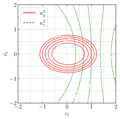
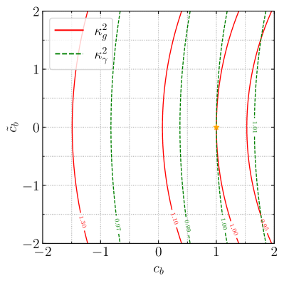
Figure 1: $\kappa_{g}^{2}$ and $\kappa_{\gamma}^{2}$ as a function of (left) $c_{t}$ and $\tilde{c}_{t}$ and (right) $c_{b}$ and $\tilde{c}_{b}$, with all other parameters fixed to their SM values. The orange star denotes the SM point.

We illustrate the numerical size of these dependencies in Fig. 1. In the left panel, we vary $c_{t}$ and $\tilde{c}_{t}$ keeping all other parameters fixed to their SM values. The gluon fusion cross section is equal to its SM value alongside an ellipsis stretching to the left of the SM point which can approximately be described by the equation $c_{t}^{2}+9/4\,\tilde{c}_{t}^{2}=1$. The gluon fusion cross section is subject to relatively large deviations from its SM prediction even in case of small deviations from the SM ellipsis. The dependence of $\kappa_{\gamma}$ on $c_{t}$ and $\tilde{c}_{t}$ is less pronounced. While $\kappa_{g}$ only has a weak sensitivity to the sign of $c_{t}$, $\kappa_{\gamma}$ is very sensitive to it as a consequence of the additional dependence on $c_{V}$.

In the right panel of Fig. 1, the dependence of $\kappa_{g}$ and $\kappa_{\gamma}$ on $c_{b}$ and $\tilde{c}_{b}$ is displayed. In comparison to the left panel, the variations of $\kappa_{g}$ and $\kappa_{\gamma}$ are much smaller for similar variations of the coupling modifiers. The gluon fusion cross section can be enhanced by about $\sim 26\%$ for a negative $c_{b}$ within the $2\,\sigma$ allowed region $-1.23\leq|c_{b}|\leq-1.08$ (see Section 4), while the di-photon decay width is reduced in this region by $\sim 3\%$. The dependence of the same quantities on $\tilde{c}_{b}$ is only at the sub-percent level. The dependence of the gluon fusion cross section on $c_{\tau}$ and $\tilde{c}_{\tau}$ is zero to very good approximation. The dependence of the di-photon decay width on $c_{\tau}$ and $\tilde{c}_{\tau}$ is even smaller than the dependence on $c_{b}$ and $\tilde{c}_{b}$, reaching maximally $\sim 1\%$ in the parameter space $0.78\leq|c_{\tau}|\leq 1.08$, $|\tilde{c}_{\tau}|\leq 0.74$ still allowed experimentally at the $2\,\sigma$ level (see Section 4).

2.2 Phenomenological models

In order to disentangle the impact of the various experimental constraints and to adjust the level of complexity in our analysis, we explore several simplified effective models with a restricted number of free parameters. We summarize them in Table 1, starting with more specific but simpler models with fewer free fit parameters before moving to more general models with up to nine free parameters. Our models are intended as phenomenological characterizations of the Higgs coupling structure and can be mapped onto concrete model realizations, as discussed below. Besides the coupling modifications, exotic Higgs decays into BSM states can occur if they are kinematically allowed. We will leave an investigation of this possibility to future work, but note that preliminary results are available in Menen:2021MScThesis. We will use the following notation for common coupling modifiers: the common quark modifier $c_{q}$ implies that all quark Yukawa couplings are modified equally, $c_{q_{i}}\equiv c_{q}$ with $q_{i}=\{u,d,c,s,t,b\}$, likewise for $\tilde{c}_{q}$; analogously for the global lepton modifiers with $c_{l_{i}}\equiv c_{l}$ of the charged leptons $l_{i}=\{e,\mu,\tau\}$ . Furthermore, we denote $f_{3}\equiv\{t,b,\tau\}$, $f_{2}\equiv\{c,s,\mu\}$, as well as $q_{u}=\{u,c,t\}$ and $q_{d}=\{d,s,b\}$.

Model	Free modifiers	$N$	Motivation	Fig(s).
1-flavor	$c_{f_{a}},\tilde{c}_{f_{a}}$ (1 fermion)	2	flavor-specific, simplest	2, 3, 9, 10
2-flavor	$c_{f_{a}},\tilde{c}_{f_{a}},c_{f_{b}},\tilde{c}_{f_{b}}$	4	interplay of 2 flavors	4, 5, 11, 12
quark	$c_{q}$, $\tilde{c}_{q}$ (all quarks)	2	NP in quark sector	6
lepton	$c_{l}$, $\tilde{c}_{l}$ (all leptons)	2	NP in lepton sector	6
quark–lepton	$c_{q}$, $\tilde{c}_{q}$, $c_{l}$, $\tilde{c}_{l}$	4	NP specific to $q$s, $l$s	15
up–down– lepton	$c_{q_{u}}$, $\tilde{c}_{q_{u}}$, $c_{q_{d}}$, $\tilde{c}_{q_{d}}$, $c_{l}$, $\tilde{c}_{l}$	6	2HDM-like distinguishing up/down-type $q$s and $l$s	15
2/3 gen.	$c_{f_{3}}$, $\tilde{c}_{f_{3}}$, $c_{f_{2}}$, $\tilde{c}_{f_{2}}$	4	NP per generation recent sensitivity to 2 gen. muon anomalies	17
fermion	$c_{f}$, $\tilde{c}_{f}$ (all fermions)	2	NP universal in fermion sector	6, 13
universal	$c_{f}\equiv c_{V},\tilde{c}_{f}$ $\tilde{c}_{V}\equiv 0$	2	mixing with a pseudoscalar (apart from $\tilde{c}_{V}=0$)	7
fermion+V	$c_{f},\tilde{c}_{f},c_{V}$ $\tilde{c}_{V}\equiv 0$	3	NP in fermion sector + gauge sector	7
fermion- vector	$c_{f},\tilde{c}_{f},c_{V},\kappa_{g},\kappa_{\gamma}$	5	separate NP contr. to fermions, to vectors, and to loops	8
up-down- lepton-vector	$c_{q_{u}},\tilde{c}_{q_{u}},c_{q_{d}},\tilde{c}_{q_{d}},$ $c_{l},\tilde{c}_{l},c_{V},\kappa_{g},\kappa_{\gamma}$	9	most general considered here	18

Table 1: Sets of coupling modifiers that are floated simultaneously. Coupling modifiers that are not listed in the second column are fixed to the SM values, $c_{X}=1$, $\tilde{c}_{X}=0$. The notation of the fermion coupling modifiers is described in the text. The vector coupling modifier is denoted as $c_{V}$ with $V=W,Z$, whereas $\kappa_{g}$ and $\kappa_{\gamma}$ are given by Eqs. 5 and 6 unless they are listed as free parameters in the second column. The third column summarizes the number $N$ of free parameters. In the fourth column, we provide a brief theory motivation behind each phenomenological model (see text for more details), while the last column references the relevant figures in which the considered model is analyzed.

The 1-flavor model is the simplest case where only the Yukawa coupling of one fermion is modified. This can be realized in models where the new physics (NP) is flavor-specific and only affects one Higgs–fermion interaction, or the modifications of other couplings are suppressed. Several models mainly affect the top quark, such as composite Higgs models [70, 71]. Here, the Higgs-dilaton potential enables a sufficiently strong first-order electroweak phase transition and the ${\cal CP}$ violation enters via the top quark Yukawa coupling, thus leading to successful baryogenesis. Bruggisser:2018mrt also considers ${\cal CP}$ violation in the charm quark Yukawa coupling. A complex tau Yukawa coupling may play an important role for lepton-flavored electroweak baryogenesis (see Section 3.3), and the recent CMS analysis [15] directly probes its ${\cal CP}$ structure. Furthermore, in the Minimal Supersymmetric Standard Model large (possibly complex) corrections to the bottom quark Yukawa coupling, parameterized by a quantity called $\Delta_{b}$, can arise especially for large values of $\mu$ and $\tan\beta$ [72, 73, 74]. Studying the muon Yukawa coupling is motivated by the observation of anomalies in its magnetic moment, $(g-2)_{\mu}$, and for bottom and strange quarks by the $B$-anomalies of $b\to s$ transitions, see e.g. Alguero:2019ptt,Aebischer:2019mlg,Arbey:2019duh. More generally, it can be motivated for all fermions to explore various scenarios where lepton universality and lepton flavor are violated, see e.g. Greljo:2021npi,Greljo:2021xmg,Crivellin:2021rbq,Darme:2021qzw. Therefore, we consider the 3-generation fermions, top quark, bottom quark, tau, and the 2-generation fermions, muon and charm quark, as well-motivated candidates for modified, complex Yukawa couplings. We treat them separately in the 1-flavor, or jointly in the 2/3 generation model (see below). We do not consider the strange quark separately due to its currently weak collider bounds [82, 83, 84] and its small contribution to baryogenesis [65].

The 2-flavor model takes the interplay of complex Yukawa couplings of two specific fermions into account. As a theory realization, one can consider models where coupling modifications are enhanced for two fermions compared to the remaining fermions while the couplings of the latter are not required to be exactly those of the SM, but only to have negligible modifications. The combination of two coupling variations allows for the (partial) cancellation of the contributions of two different fermions to, e.g., an electric dipole moment. Combinations of two fermions from the third generation lead to an interesting interplay in the LHC constraints. Another relevant combination is to include the electron as one of the selected fermions. Large variations of the electron Yukawa coupling including an imaginary part can be realized e.g. in the 2HDM [85].

The quark model assumes that all quark couplings are modified universally. Such a scenario can arise when new bosonic particles $X$ couple universally to any quark in a loop as a correction to the SM Yukawa coupling, e.g. in a triangle diagram to each $hq\bar{q}$ vertex containing one $X$ and two quarks or two $X$ and one quark. As the experimental constraints on the Yukawa couplings of the top and bottom quarks are the tightest, in this model the lighter quarks will be simultaneously constrained by the strong bounds on the third generation, more strongly than if they were independent.

Likewise, the lepton model assumes a universal modification of all lepton Yukawa couplings by New Physics that couples exclusively or dominantly to charged leptons while its effects on the quarks (and neutrinos) is negligible. One possibility is a $U(1)_{L}$ extension of gauged lepton number [86].

In contrast, in the quark-lepton model, we consider NP that affects quarks and leptons, but separately. Here, models with several new particles coupling either to quarks or to leptons, or with one new particle coupling differently to quarks and leptons are a possible realization. An example of the latter case is the $B-L$ extension of the SM by gauging the difference of baryon ($B$) and lepton ($L$) number. As all quarks have the same charge of $z_{q}=1/3$ under the new gauge group $U(1)_{B-L}$ and all leptons have $z_{l}=-1$, the predicted $Z^{\prime}$ boson couples more strongly to leptons than to quarks by a factor of $-3$. As the $Z^{\prime}$ can modify the $l\bar{l}h$ and $q\bar{q}h$ vertices, this model motivates the separate fit of a quark and a lepton Yukawa coupling modifier.

In the up-down-lepton  model, the NP couples to the fermions according to their category: up-type or down-type quarks, and charged leptons. This is inspired by the Two-Higgs Doublet Model (2HDM) where — according to its type — all or two of these three categories are summarized by shared Yukawa coupling modifiers. In the 2HDM, however, also the vector couplings are modified (albeit weaker than the couplings to fermions). Furthermore, two instead of three independent fermion coupling modifiers would give tighter constraints. Nevertheless, this model can be considered as a prototype for more specific choices.

The 2/3 generation model distinguishes changes of the Yukawa couplings in the third generation from the second. This is motivated by scenarios where the NP couples differently to each generation, possibly also to the first generation, but there is not sufficient experimental sensitivity to the latter yet. Therefore we restrict the analysis to the heavier two generations. In view of the muon and $B$-meson anomalies this setup is not only motivated by theory, but also by recent data [78, 79, 80, 81]. For example, a $U(1)^{\prime}$ extension of the SM with generation-dependent couplings [87] can account for several $B$-anomalies.

In the fermion model, all fermions are modified by the same coupling modifiers, see e.g. Li:2012ku about universal Yukawa modifiers.

In the universal model, the real parts of the Higgs couplings to all fermions and the vector bosons $W,Z$ are varied universally. In addition, a universal imaginary Yukawa coupling modifier is included as in the fermion model. This can be realized in the relaxion framework [89] where the relaxion as a light pseudoscalar scans the Higgs mass and stops its evolution at a local minimum of its potential that breaks ${\cal CP}$. As a consequence, the relaxion mixes with the Higgs boson [90, 91, 92], and the Higgs couplings to all fermions and the massive vector bosons are reduced by the universal mixing angle $c_{f}=c_{V}=\cos\theta$. Furthermore, Minimal Composite Higgs models (MCHM, see e.g. Refs. [93, 94, 95, 96, 97]) predict the Higgs couplings to vector bosons to be reduced by a factor of $c_{V}=\sqrt{1-\xi}$, where $\xi=v^{2}/f^{2}$ is the squared ratio of the electroweak vacuum expectation value $v$ and the scale $f$ of global symmetry breaking. The Yukawa coupling modifiers depend on the chosen symmetry breaking pattern; in the minimal composite Higgs model of $SO(5)/SO(4)$ with the top partner in the spinorial representation, denoted as MCHM₄, also the Higgs–fermion couplings are reduced by $c_{f}=\sqrt{1-\xi}$ [94]. Furthermore, in the Twin Higgs framework [98], the coupling of the observed Higgs boson to SM particles is suppressed by a universal factor $c_{f}=c_{V}=\cos\left(\frac{v}{\sqrt{2}f}-\theta\right)$ [99], where $\theta$ is the mixing angle between the observed and a heavier Higgs boson and $f$ is the energy scale that breaks the global $SU(4)\times U(1)$ symmetry. Hence, there are several examples of a universal modifier model.

The fermion+V model, in contrast, distinguishes between universal modifiers for the fermions $f$ and vector bosons $V$. In addition, we allow for BSM contributions to the loop-induced couplings of the Higgs bosons to gluons and photons. In the Minimal Composite Higgs Model of $SO(5)/SO(4)$ with the top partner in the fundamental representation, denoted as MCHM₅, the Yukawa coupling modifiers are predicted to differ from $c_{V}$ (see above) and are given by $c_{f}=\frac{1-2\xi}{\sqrt{1-\xi}}$ [95, 96]. The fermion-vector model can also originate from the Two-Higgs Doublet Model (2HDM) of Type I where all fermions couple to the second Higgs doublet $H_{2}$ such that the Yukawa couplings of the lighter neutral Higgs boson are modified by $c_{f}=\cos\alpha/\sin\beta$ with respect to the SM Higgs boson. The couplings to vector bosons are modified by $c_{V}=\sin(\alpha-\beta)$ where $\alpha$ is the mixing angle of the neutral Higgs states, and $\tan\beta=v_{2}/v_{1}$ is the ratio of the vacuum expectation values of the Higgs doublets.

The fermion-vector model extends the fermion+V model by additional modifiers for Higgs production via gluon fusion and the Higgs decay into two photons. These can be used to parameterize the effect of additional colored or electrically charged BSM states like the top partner in the Minimal Composite Higgs Model.

The up-down-lepton-vector model is the most general model considered in this work. It allows one to vary the three types of fermion couplings as well as the real parts of the tree-level coupling to the massive gauge bosons, and independently the loop-induced couplings to gluons and photons.

3 Constraints

In this Section, we describe the different types of measurements used to constrain the models introduced in Section 2.

3.1 LHC measurements and constraints

Included data

In order to derive LHC constraints on ${\cal CP}$-odd admixtures in the Higgs couplings we fit Higgs boson rates as measured by ATLAS and CMS with a focus on those involving fermions. We use the same set of observables as in Bahl:2020wee which includes in particular the inclusive measurements of $t\overline{t}H$ in the multi-lepton [100, 101, 102, 103, 104, 105], di-photon [19, 20, 106, 107] and $b\overline{b}$ decay channels [108, 109, 110, 111, 112, 113] and the measurements for $ZH$ production in bins of Higgs transverse momentum ($p_{T}$) [114, 115, 106], which are sensitive to the ${\cal CP}$ nature of the top quark Yukawa interaction.

We furthermore include the latest experimental results on $H\to\mu^{+}\mu^{-}$ [116, 117] and $H\to c\bar{c}$ [118, 119, 120] measurements from ATLAS and CMS. The charm quark Yukawa coupling has not been observed yet at the LHC, but the searches for $H\to c\bar{c}$ decays [119, 118, 120] in the $VH(c\bar{c})$ channel with charm tagging constrain $|g_{c}|<8.5$ at the 95% CL. This direct limit includes the effect of a modified charm quark Yukawa coupling on the partial width $\Gamma(H\to c\bar{c})$ as well as on the total Higgs width $\Gamma_{h}^{\rm{tot}}$, see Eq. (8). Other measurements involving the charm quark Yukawa coupling are not as sensitive to $|g_{c}|$ as the indirect bound via ${\rm{BR}}(H\to\gamma\gamma)$. Finally, we add the CMS analysis of the ${\cal CP}$ structure of the tau Yukawa coupling [15]. The ${\cal CP}$ analysis in the $\tau^{+}\tau^{-}$ final state is the only measurement targeting a Higgs–fermion coupling based on a dedicated ${\cal CP}$-odd observable, where the ${\cal CP}$-violating phase $\alpha_{\tau}$ is directly inferred by measuring the angle between the decay planes of the two tau leptons. It is included in the list of measurements by adding the $\chi^{2}$ contribution corresponding to the data of hepdata.104978.v1/t4. We refer to these measurements as the “LHC data set” in the following.

Several ${\cal CP}$ sensitive measurements could not be included such as the $p_{T}$-binned STXS measurement of $t\overline{t}H$ [129] as it relies on a separation of $tH$ from $t\bar{t}H$ production based on the assumption of SM-like kinematics. As shown in Bahl:2020wee, this assumption does not hold in the presence of a ${\cal CP}$-odd Yukawa coupling. We also did not include analyses using full Run 2 data fitting the rates of the $t\bar{t}H$, $tH$ and $tWH$ processes in the Higgs to di-photon decay channel [130, 131], as the data is not available in a sufficiently model-independent format, see the discussion in Bahl:2020wee.

In order to include the LHC constraints, we use HiggsSignals (version 2.5.0) [132, 133, 134, 135] which incorporates the available inclusive and differential Higgs boson rate measurements from ATLAS and CMS from Run 2 [108, 109, 100, 101, 102, 106, 136, 103, 115, 19, 137, 110, 111, 112, 113, 138, 139, 104, 105, 107, 140], as well as the combined measurements from Run 1 [3]. On top of the channels currently implemented in HiggsSignals we included the most recent results on $H\to c\bar{c},\mu^{+}\mu^{-},\tau^{+}\tau^{-}$ [119, 118, 120, 116, 117, 15] as described above.

The experimental measurements are implemented with correlation matrices and detailed information about the composition of the signal in terms of the various relevant Higgs boson production and decay processes. If this information is not available (e.g. in the recent CMS $H\to\tau^{+}\tau^{-}$ ${\cal CP}$ study), the signal is assumed to be composed of the relevant Higgs processes with equal acceptances, and only correlations of the luminosity uncertainty (within one experiment) and theoretical rate uncertainties are taken into account. Further details on the cross section calculations and the fit implementation can be found in [48].

Based on this large collection of measurements and the predicted cross sections for different parameter choices, HiggsSignals is used to determine favored regions in parameter space by calculating the $\chi^{2}$ difference, $\Delta\chi^{2}\equiv\chi^{2}-\chi^{2}_{\text{min}}$, with $\chi^{2}_{\text{min}}$ being the minimal $\chi^{2}$ value found at the best-fit point. The parameter spaces are sampled using a combination of two different types of Markov Chain Monte Carlo samplers. Alongside a common Metropolis Hastings approach [141, 142], a realization of the Stretch Move Algorithm in Emcee [143, 144] was used. We found this method to provide the best convergence behaviour. Furthermore, it ensures that parameter spaces in which regions of high likelihood are either narrow or separated by large potential barriers are sampled efficiently [69].

While for gluon fusion and the Higgs decay into two photons fit formulas are available at leading-order (LO) in analytic form, this is not the case for other Higgs boson production processes. For calculating cross-sections in the “Higgs characterization model” [68, 145, 29], we use MadGraph5_aMC@NLO 2.7.0 [146] with Pythia 8.244 [147] as parton shower employing the A14 set of tuned parameters [148]. The cross-sections are computed at LO in the five-flavor scheme and rescaled to the state-of-the-art SM predictions reported in Ref. [149].

Approximate dependences of branching ratios on coupling modifiers

For an arbitrary combination of Yukawa coupling modifications, but $c_{V}=1$, the branching ratios into a pair of fermions $f\bar{f}$ are given by

$${\rm{BR}}_{f} =\frac{g_{f}^{2}\Gamma_{f}^{\text{SM}}}{\sum_{f^{\prime}}g_{f^{\prime}}^{2}\Gamma_{f^{\prime}}^{\text{SM}}+\Gamma^{\text{SM}}(H\to VV)+\Gamma(H\to{\text{NP}})}\,,$$ (7)

where $g_{f}$ is defined in Eq. 2, and $\Gamma_{f}^{\text{SM}}=\Gamma^{{\text{SM}}}(h\to f\bar{f})$ is the partial width in the SM, and the sum over $f^{\prime}$ includes all fermions. Therefore, in the case of the modification of only one Yukawa coupling of fermion $f$ and no decay into new particles, the branching ratio into $f\bar{f}$ can be expressed as

$${\rm{BR}}_{f} =\frac{g_{f}^{2}\Gamma_{f}^{\text{SM}}}{g_{f}^{2}\Gamma_{f}^{\text{SM}}+\Gamma_{\rm{tot}}^{\text{SM}}-\Gamma_{f}^{\text{SM}}}=\frac{g_{f}^{2}{\rm{BR}}_{f}^{\text{SM}}}{(g_{f}^{2}-1){\rm{BR}}_{f}^{\text{SM}}+1}\,,$$ (8)

where ${\rm{BR}}_{f}^{\text{SM}}$ denotes the branching ratio in the SM and $\Gamma_{\rm{tot}}^{\text{SM}}$ denotes the total Higgs width in the SM. Hence, a particular measured value of the branching ratio, ${\rm{BR}}_{f}^{\rm{exp}}$, yields a circle in the $c_{f},\,\tilde{c}_{f}$ plane of squared radius

$$g_{f}^{2}\equiv c_{f}^{2}+\tilde{c}_{f}^{2}=\frac{{\rm{BR}}_{f}^{\rm{exp}}}{{\rm{BR}}_{f}^{\text{SM}}}\,\cdot\,\frac{{\rm{BR}}_{f}^{\text{SM}}-1}{{\rm{BR}}_{f}^{\rm{exp}}-1}\,.$$ (9)

This results in rings corresponding to the upper and lower bound on ${\rm{BR}}_{f}^{\rm{exp}}$ if the constraints are dominated by the decay rate information, see Figs. 2 and 3.

Likewise, we consider the modification of one Yukawa coupling and its impact on the $H\to\gamma\gamma$ decay via the modification of the total Higgs width, i.e. the free coupling modifiers $c_{f}$, $\tilde{c}_{f}$ and $\kappa_{\gamma}$,

$${\rm{BR}}_{\gamma}=\frac{\kappa_{\gamma}^{2}\Gamma_{\gamma}^{\text{SM}}}{\Gamma_{f}^{\text{SM}}(g_{f}^{2}-1)+\Gamma_{\gamma}^{\text{SM}}(\kappa_{\gamma}^{2}-1)+\Gamma_{\rm{tot}}^{\text{SM}}}\,.$$ (10)

Here. $\Gamma_{\gamma}^{\text{SM}}\equiv\Gamma^{\text{SM}}(H\to\gamma\gamma)$ is the SM value of the partial width into a pair of photons. This implies that $g_{f}^{2}$ can be expressed as

$$g_{f}^{2}\equiv c_{f}^{2}+\tilde{c}_{f}^{2}=1+\frac{1}{{\rm{BR}}_{f}^{\text{SM}}}\cdot\left[{\rm{BR}}_{\gamma}^{\text{SM}}\cdot\,\left(\frac{\kappa_{\gamma}^{2}}{{\rm{BR}}_{\gamma}^{\rm{exp}}}-(\kappa_{\gamma}^{2}-1)\right)-1\right]\,,$$ (11)

where ${\rm{BR}}_{\gamma}^{\rm{exp}}\equiv{\rm{BR}}^{\rm{exp}}(H\to\gamma\gamma)$ denotes the measured branching ratio of the Higgs boson into photons, and ${\rm{BR}}_{\gamma}^{\text{SM}}$ is its prediction in the SM. As discussed in Sec. 2.1, $\kappa_{\gamma}$ can be calculated as a result of $c_{f}$, $\tilde{c}_{f}$, see Eq. 6, it can be floated independently, or it can be set to its SM value of 1. Unless $\kappa_{\gamma}$ is treated as depending on $c_{f}$, $\tilde{c}_{f}$, Eq. (11) shows that also the constraint from measuring ${\rm{BR}}_{\gamma}={\rm{BR}}_{\gamma}^{\rm{exp}}$ leads to a circular ring in the $c_{f}$, $\tilde{c}_{f}$ plane. If one further assumes $\kappa_{\gamma}=1$ (in case of a negligible contribution of the considered fermion $f$ to $\kappa_{\gamma}$), Eq. (11) can be simplified to

$$g_{f}^{2}\Big{|}_{\kappa_{\gamma}=1}=1+\frac{1}{{\rm{BR}}_{f}^{\text{SM}}}\cdot\left[\frac{{\rm{BR}}_{\gamma}^{\text{SM}}}{{\rm{BR}}_{\gamma}^{\rm{exp}}}-1\right]\,.$$ (12)

3.2 EDM constraint

Several EDMs are sensitive to the ${\cal CP}$ nature of the Higgs boson. The most sensitive ones are the electron EDM (eEDM) and the neutron EDM (nEDM). Besides the experimental results [54, 55], much work has been done to provide precise theory predictions [56, 57, 59, 58, 60, 150, 151, 152].

The main focus of the present work are the LHC constraints. Therefore, we take into account only constraints from the eEDM, which is theoretically the cleanest EDM. Since the various EDMs are independent measurements, taking into account additional EDM measurements (e.g. the nEDM) could potentially tighten the constraints on the Higgs ${\cal CP}$ nature. Correspondingly, our EDM constraint, based only on the eEDM, can be regarded as conservative.

The dominant contribution from ${\cal CP}$-violating Higgs–fermion couplings to the eEDM appear at the two-loop level in the form of Barr-Zee diagrams. For their evaluation, we make use of the analytical results given in Brod:2013cka,Altmannshofer:2015qra,Panico:2018hal,Altmannshofer:2020shb. While we use the full analytical expressions for our numerical analysis, these expressions can also be translated into a simple numerical formula allowing to easily assess the relative importance of the various ${\cal CP}$-violating Higgs couplings,

$$\frac{d_{e}}{d_{e}^{\text{ACME}}}={} c_{e}\left(870.0\tilde{c}_{t}+3.9\tilde{c}_{b}+2.8\tilde{c}_{c}+0.01\tilde{c}_{s}+8\cdot 10^{-5}\tilde{c}_{u}+7\cdot 10^{-5}\tilde{c}_{d}+3.4\tilde{c}_{\tau}+0.03\tilde{c}_{\mu}\right)$$

$$+\tilde{c}_{e}\left(610.1c_{t}+3.1c_{b}+2.3c_{c}+0.01c_{s}+7\cdot 10^{-5}c_{u}+6\cdot 10^{-5}c_{d}+2.8c_{\tau}+0.02c_{\mu}\right.$$

$$\left.\hskip 28.45274pt-1082.6c_{V}\right)$$

$$+2\cdot 10^{-6}c_{e}\tilde{c}_{e}.$$ (13)

Here, $d_{e}^{\text{ACME}}=1.1\cdot 10^{-29}e\,\rm{cm}$ is the 90% CL upper bound on the eEDM obtained by the ACME collaboration [54]. Correspondingly, a parameter point is regarded as excluded at the 90% CL if $|d_{e}/d_{e}^{\text{ACME}}|>1$.

In general, the contributions of two or more particles to $d_{e}$ can cancel each other, partially or fully. Especially, Eq. 13 shows that a ${\cal CP}$-violating top-Yukawa coupling can induce a large contribution to the eEDM, depending on the value of $|c_{e}|$. For a non-zero value of $\tilde{c}_{e}$, large additional contributions proportional to $c_{t}$ and $c_{V}$ can occur. As we will investigate below (see also Fuyuto:2019svr), these two types of potentially large contributions can cancel each other. Currently, the most constraining experimental bound on the electron-Yukawa coupling is from the ATLAS Run 2 measurement [153] and yields $g_{e}\leq 268$ at 95% CL. Since the current bound is too loose for meaningful fit results, we will restrict to the SM values $c_{e}=1$, $\tilde{c}_{e}=0$ in the analyses presented in this work unless otherwise stated. On the other hand, there exists no experimental lower bound on the electron-Yukawa coupling, and also in the future it will remain very difficult to establish evidence of a non-zero electron Yukawa coupling. Thus, in case $c_{e}$ and $\tilde{c}_{e}$ are very small, i.e. in particular if $c_{e}$ is much below the SM value, the BSM contributions to $d_{e}$ would be heavily suppressed and therefore the impact of the limit on the eEDM would be drastically reduced.

3.3 BAU constraint

The baryon asymmetry in the universe, $Y_{B}$, was measured by PLANCK to be [154]

$$Y_{B}^{\text{obs}}=(8.59\pm 0.08)\times 10^{-11}\,.$$ (14)

The description of the BAU requires additional sources for ${\cal CP}$ violation beyond the CKM phase that is present in the SM. An attractive framework for explaining the BAU is electroweak baryogenesis (EWBG), for reviews see e.g. Refs. [155, 53, 156, 51]. For EWBG a non-vanishing baryon number density is achieved during the electroweak phase transition, implying that the mechanism can potentially be tested with Higgs processes at the LHC. In the phase transition, bubbles of the broken phase with $v\neq 0$ form, whereas the electroweak symmetry is unbroken outside of the bubbles; the bubbles expand until the universe is filled by the broken phase. Across the bubble wall, ${\cal CP}$-violating interactions create a chiral asymmetry that is partially washed out by the ${\cal CP}$-even interactions and the sphalerons. A part of the generated chiral asymmetry diffuses through the bubble wall into the symmetric phase where it is converted into a baryon asymmetry by the weak sphaleron process. Then the expanding bubble wall reaches the region where the baryon asymmetry was created, which is then maintained in the broken phase.

While the experimental precision of the PLANCK measurement in Eq. (14) is around 1%, the theoretical uncertainties of predicting the BAU in different models of electroweak baryogenesis are up to now much larger. The largest uncertainty can be associated with the deviations between different approaches that are employed for calculating the source term for the baryon asymmetry, namely the perturbative so-called vev-insertion-approximation (VIA) [50, 157, 158, 159, 160, 161], and the semi-classical Wentzel-Kramer-Brillouin (WKB) approach [162, 163, 164, 165, 166, 167, 168]. While both formalisms yield similar outcomes of the baryon asymmetry for an equivalent source term, they largely differ in the calculation of the source term [169, 170]. For a systematic comparison of both approaches see in particular Cline:2021dkf. The perturbative approach starts with Green’s functions in a Closed Time Path formalism. The interaction rates and the ${\cal CP}$-violating source term are computed from the self-energies, and the vev-dependent contributions to the particle masses are included as a perturbation. In contrast, the WKB approach starts with the Boltzmann equations, and the interactions are described as semi-classical forces in the plasma. There is a long-standing controversy in the literature about which approach to apply. Recent studies have shown that the VIA leads to systematically higher predictions of the amount of the baryon asymmetry due to an additional derivative in the WKB source term [169, 170, 171]. This has been evaluated for a source term from a complex tau Yukawa coupling with an additional singlet scalar term of dimension 5 and a maximal relative ${\cal CP}$-violating phase between the terms of dimension 4 and 5. The evaluation furthermore assumed the benchmark value of the wall velocity of $v_{w}=0.05$ (as used in our work), and a wall thickness of $L_{w}=5/T$ with $T=88\,\,\mathrm{GeV}$ (i.e. about half of the value adopted in our work, $L_{w}=0.11\,\mathrm{GeV}^{-1}$). Using these parameters Cline:2021dkf reports a discrepancy of about five orders of magnitude between the VIA and WKB approach. For a charm quark source, the discrepancy is found to be around one order of magnitude. The discrepancy for a top quark source was found to reach a factor of 10 – 50 depending on $v_{w}$ and $L_{w}$ [169]. Furthermore, the applicability of the VIA depends on the width of the bubble wall [172]. Another recent study [171] stresses the impact of thermal corrections at the one-loop level, raising concerns about the validity of the VIA because of an apparently vanishing source term, but also pointing to potential open issues in the WKB approach.

Besides the large differences between the VIA and WKB approaches, which we treat as a theoretical uncertainty, there are also smaller theoretical uncertainties that are inherent to the individual approaches. We comment here on the case of the VIA approach. Theoretical uncertainties of this kind arise within the VIA approach from the perturbative expansion and from the not precisely known bubble parameters. Especially the NLO terms in the VIA can be large as was shown in Ref. [173], around $\mathcal{O}(1)$ for the top quark, but at the sub-per-mille level for the bottom quark and the tau lepton because of their smaller Yukawa couplings. In addition, the prediction of $Y_{B}$ depends on the bubble wall properties, in particular on the bubble wall width, $L_{w}$, and velocity, $v_{w}$, as well as on the bubble wall profile (i.e. the variation of the vev from the inner to the outer bubble wall). In contrast to the long-standing expectation that small velocities should lead to higher $Y_{B}$, EWBG can also be successful with supersonic bubble walls, as shown recently in Refs. [174, 170].

In view of the described uncertainties affecting the prediction of the BAU, we adopt the following strategy for assessing the impact of the BAU constraint. As the predictions based on the VIA approach tend to yield significantly higher values for $Y_{B}$ than the WKB approach, we employ the VIA approach for obtaining an “optimistic” reference value for the BAU. Specifically, we apply the bubble wall parameters $v_{w}$ and $L_{w}$ as in the benchmark used in deVries:2018tgs,Fuchs:2020uoc,Fuchs:2020pun,Shapira:2021mmy such that they yield values of $Y_{B}^{\text{VIA}}$ for the given couplings that are near the maximally possible values. Accordingly, the obtained value for $Y_{B}^{\text{VIA}}$ corresponds to an approximate upper bound on $Y_{B}$ .For this reason we do not attempt to show confidence levels, but restrict ourselves to displaying the nominal value of the BAU. We regard a parameter point as disfavored by the observed BAU if the value predicted for $Y_{B}$ in the (optimistic) VIA approach is such that $Y_{B}^{\text{VIA}}/Y_{B}^{\text{obs}}<1$. On the other hand, values with $Y_{B}^{\text{VIA}}/Y_{B}^{\text{obs}}>1$ may well be phenomenologically viable if the VIA approach turns out to overestimate the predicted value of $Y_{B}$. We therefore indicate the parameter regions fulfilling $Y_{B}^{\text{VIA}}/Y_{B}^{\text{obs}}\geq 1$ as those that are favored by the observed BAU. For illustration, contour lines for fixed values of $Y_{B}^{\text{VIA}}/Y_{B}^{\text{obs}}$ are shown in our plots.

The prediction for $Y_{B}^{\text{VIA}}/Y_{B}^{\text{obs}}$ consists of the contributions from the different fermions that are proportional to the respective parameters $\tilde{c}_{f}$. We use the evaluations from Refs. [63, 65] of all fermions as given by the simple formula

$$Y_{B}^{\text{VIA}}/Y_{B}^{\text{obs}}={} 28\tilde{c}_{t}-0.2\tilde{c}_{b}-0.03\tilde{c}_{c}-2\cdot 10^{-4}\tilde{c}_{s}-9\cdot 10^{-8}\tilde{c}_{u}-4\cdot 10^{-7}\tilde{c}_{d}$$

$$-11\tilde{c}_{\tau}-0.1\tilde{c}_{\mu}-3\cdot 10^{-6}\tilde{c}_{e},$$ (15)

where the coefficients have been evaluated by employing the benchmark parameters as defined in Fuchs:2020uoc,Shapira:2021mmy.

4 Results

In this Section, we present the results of our numerical fits for specific realizations of the scenarios defined in Section 2. First, we focus on the constraints set by LHC measurements (supplementary results are provided in Appendix A). In a second step, we investigate the interplay with the eEDM constraint and the obtainable BAU in the VIA.

4.1 LHC results

In the following, all presented results are based on the LHC data set, defined in Section 3.1, except for Fig. 2, where the CMS $H\to\tau^{+}\tau^{-}$ ${\cal CP}$ measurement is excluded. Accordingly, the $\chi^{2}$ value of the SM point in the plots below is always $\chi^{2}_{\mathrm{SM}}=89.36$ (except for Fig. 2).

4.1.1 1-flavor models

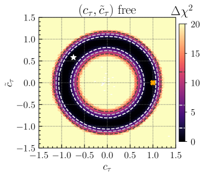
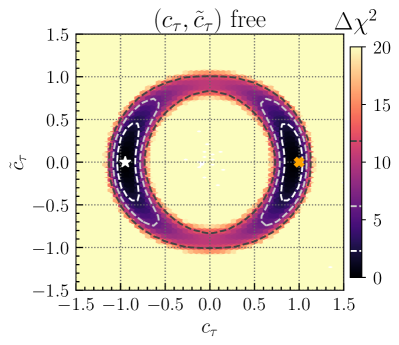
Figure 2: Results of fits to the LHC measurements in the ($c_{\tau}$, $\tilde{c}_{\tau}$) parameter plane where in the set of input measurements the CMS $H\to\tau^{+}\tau^{-}$ ${\cal CP}$ result [15] is (a) omitted and (b) included. The coupling modifiers $c_{\tau}$ and $\tilde{c}_{\tau}$ are treated as free parameters while all other parameters are fixed to their SM values. The color corresponds to the profile $\Delta\chi^{2}$ of the global fit, and the $1\sigma$, $2\sigma$ and $3\sigma$ confidence regions are shown as white, light-gray and dark-gray dashed contours, respectively. The best-fit point and the SM case are marked by a white star and an orange cross, respectively.

$\tau$ Yukawa coupling

We first investigate the two-dimensional plane of the ${\cal CP}$-even and ${\cal CP}$-odd tau Yukawa coupling modifiers, $c_{\tau}$ and $\tilde{c}_{\tau}$, respectively, treating only these two parameters as free-floating in the fit. The tau Yukawa coupling is constrained by measurements of $H\to\tau^{+}\tau^{-}$ decays, and by measurements of $H\to\gamma\gamma$ decay rates in which tau leptons enter at the loop-level. In practice, the former dominates the current constraint due to the predominance of the $W$ boson, top quark and bottom quark loop diagrams in $H\to\gamma\gamma$ decays. In the absence of ${\cal CP}$-sensitivity, one expects $H\to\tau^{+}\tau^{-}$ decay rate measurements to show a dependence on $c_{\tau}^{2}+\tilde{c}_{\tau}^{2}$ forming a ring-shaped constraint (see Eq. 11). This pattern is observed in Fig. 2, where only the inclusive $H\to\tau^{+}\tau^{-}$ decay rate but not the recent CMS $H\to\tau\tau$ ${\cal CP}$ measurement [15] is included as input to the fit. The current precision of the $H\to\gamma\gamma$ measurement has no visible effect on the ring structure. Furthermore, there is no statistically significant sensitivity to the precise location of the best-fit point (shown as a white star in the plots) within the ring. We find $\chi^{2}_{\rm{min}}=87.48$ for the best-fit point, while the SM point ($c_{\tau}=1,~{}\tilde{c}_{\tau}=0$, shown as an orange cross in the plots) has $\chi^{2}_{\mathrm{SM}}=88.33$. Fig. 2 shows the result based on the full set of input measurements, i.e. including the CMS $H\to\tau^{+}\tau^{-}$ ${\cal CP}$ measurement [15]. This experimental result excludes large $|\tilde{c}_{\tau}|$ values (i.e. $|\tilde{c}_{\tau}|<0.75$ at the 95% CL) in the fit, as expected from the unique sensitivity brought by this analysis. The best-fit point has $\chi^{2}_{\rm{min}}=87.63$. The fact that the best-fit point is located at a negative rather than a positive $c_{\tau}$ value is again not statistically significant and only corresponds to a small difference of $\Delta\chi^{2}=0.23$ with respect to the best-fit point at $c_{\tau}>0$. The SM point is located within the 1$\sigma$ area.

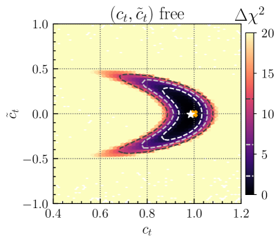
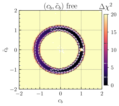
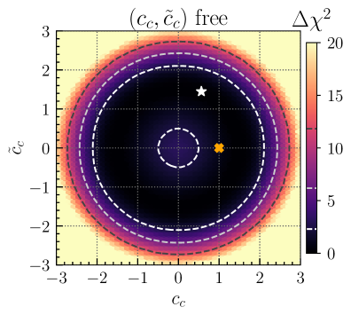
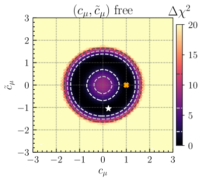
Figure 3: Results of fits to the LHC measurements in the (a) ($c_{t}$, $\tilde{c}_{t}$), (b) ($c_{b}$, $\tilde{c}_{b}$), (c) ($c_{c}$, $\tilde{c}_{c}$) and (d) ($c_{\mu}$, $\tilde{c}_{\mu}$) parameter planes. In each case, the two parameters shown in the plot are free-floating while all the other parameters are set to their SM values. The legend corresponds to the one in Fig. 2.

Quark and $\mu$ Yukawa couplings

We now consider similar two-dimensional planes for the top quark, the bottom quark, the charm quark and the muon, see Fig. 3. The LHC data set is included for these fits, and in each case only the two plotted parameters are free-floating, while all the others are set to their SM values. For a discussion of the correlation between the top quark coupling modifiers that is displayed in Fig. 3 we refer to Bahl:2020wee. In that fit, the best-fit point, with $\chi^{2}_{\rm{min}}=89.28$, is close to the SM point.

The bottom quark Yukawa coupling is constrained predominantly by measurements of $H\to bb$ decays. The rate measurement, similarly to $H\to\tau^{+}\tau^{-}$, depends on $c_{b}^{2}+\tilde{c}_{b}^{2}$, but in this case no additional ${\cal CP}$ measurement is available, and consequently the ring-shape constraint is preserved. The fit result is shown in Fig. 3. In contrast to Fig. 2 we observe that the region corresponding to $c_{b}<0$ is disfavored. This is mostly because of the significant increase of the $ggH$ production cross section in this region, caused by the positive interference with the top quark contribution ($ggH$ production is enhanced by $\sim 23\%$ for $c_{b}=-1$). Note also that due to the same effect, the ring structure of the one- and two-sigma regions are slightly asymmetric around $c_{b}=0$. The best-fit point has $\chi^{2}_{\rm{min}}=89.35$.

The results for the charm quark Yukawa coupling are shown in Fig. 3. While the direct search for $VH,~{}H\to c\overline{c}$ yields a limit on $|g_{c}|$ (see Eq. 2) of $|g_{c}|<8.5$ at the 95% CL, the precise measurement of ${\rm{BR}}(H\to\gamma\gamma)$ sets tighter constraints on $|g_{c}|$ due to the modification of the total width. Therefore, our global fit is dominated by this indirect constraint. The result shown in the plot corresponds to $|g_{c}|<2.45$ at the 95% CL, in agreement with the estimate in Eq. (10). The best-fit point has $\chi^{2}_{\rm{min}}=89.00$. Similar to Fig. 2, its precise location inside the ring is not statistically significant.

Fig. 3 shows the results for the muon Yukawa coupling. Since the contribution of the muon loop to ${\rm{BR}}(H\to\gamma\gamma)$ is negligible, the constraints on $c_{\mu}$ and $\tilde{c}_{\mu}$ stem from the $H\to\mu^{+}\mu^{-}$ decay. The searches for this decay at ATLAS and CMS [116, 117] reach a higher sensitivity compared to the case of the charm quark, reducing the ring width such that the point with $c_{\mu}=0,~{}\tilde{c}_{\mu}=0$ is outside the $2\sigma$ region, but still inside the $3\sigma$ region. The best-fit point has $\chi^{2}_{\rm{min}}=89.21$, and again there is no significant sensitivity to its precise location.

4.1.2 2-flavor models

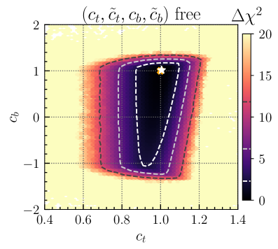
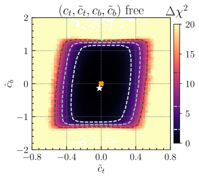
Figure 4: Fit results in the (a) ($c_{t}$, $c_{b}$) and (b) ($\tilde{c}_{t}$, $\tilde{c}_{b}$) parameter planes. In each case, the ${\cal CP}$-even and ${\cal CP}$-odd parts of the couplings shown in the plot are free-floating while all the other parameters are set to their SM values. The legend corresponds to the one in Fig. 2.

Next, we turn to scenarios in which coupling modifiers of two flavors are free-floating simultaneously. The associated results for top and bottom quarks, top quark and tau lepton, and bottom quark and tau lepton are presented in Figs. 4 and 5.

$\boldsymbol{t+b}$ Yukawa couplings

The constraints on the Higgs–top-quark and Higgs–bottom-quark Yukawa coupling modifiers, see Fig. 4, are partially correlated because $ggH$ measurements have an impact on both of them. This opens the possibility of partial cancellations in the BSM contributions, which can lead to a SM-like $ggH$ production cross section even though each coupling deviates significantly from the SM. In particular, low $c_{b}$ values can be compensated by a slightly reduced $c_{t}$ parameter (with respect to the SM case), see Eq. 5. A similar cancellation effect happens in the case of the ${\cal CP}$-odd coupling modifiers, but is suppressed due to the smaller corresponding interference term, as a consequence of the more stringent constraints on $\tilde{c}_{t}$. The best-fit point corresponds to $\chi^{2}_{\rm{min}}=89.28$.

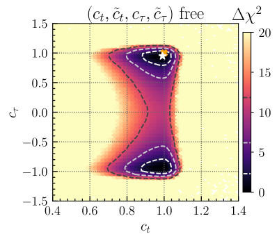
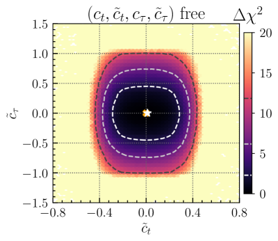
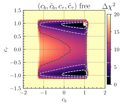
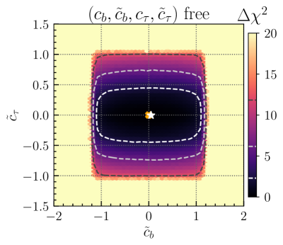
Figure 5: Results of fits to the LHC measurements in the (a) ($c_{t}$, $c_{\tau}$), (b) ($\tilde{c}_{t}$, $\tilde{c}_{\tau}$), (c) ($c_{b}$, $c_{\tau}$), and (d) ($\tilde{c}_{b}$, $\tilde{c}_{\tau}$) parameter planes. In each case, the ${\cal CP}$-even and ${\cal CP}$-odd parts of the couplings shown in the plot are free-floating while all the other parameters are set to their SM values. The legend corresponds to the one in Fig. 2.

$\boldsymbol{\tau+t,~{}\tau+b}$ Yukawa couplings

For models with free top quark and tau Yukawa couplings, see Figs. 5 and 5, and bottom quark and tau Yukawa couplings, see Figs. 5 and 5, the only source of potential correlation originates from $H\to\gamma\gamma$ decays and is very limited due to the small contribution of the Higgs–tau-lepton Yukawa coupling to this process. In Fig. 5, the constraints on $c_{b}$ at $c_{\tau}=1$ differ from the ones previously shown in Fig. 3 and Fig. 4. This is a direct effect of the CMS $H\to\tau^{+}\tau^{-}$ analysis, where – as noted in the discussion of Fig. 2 – the $\chi^{2}_{\rm{min}}$ value of the best-fit point is slightly lower than the one of the SM point, $\chi^{2}_{\mathrm{SM}}=89.36$. The best-fit point for the free top-quark (bottom-quark) and tau-lepton couplings corresponds to 87.53 (87.54). This difference of $\Delta\chi^{2}\approx 1.8$ between the best-fit point and the SM point gives rise to a corresponding increase of the $\Delta\chi^{2}$ value compared to scenarios in which $c_{\tau}=1$ and $\tilde{c}_{\tau}=0$ (as in Figs. 3 and 4). It has also a small impact on the $c_{t}$ constraint in Fig. 5, though the effect is barely visible.

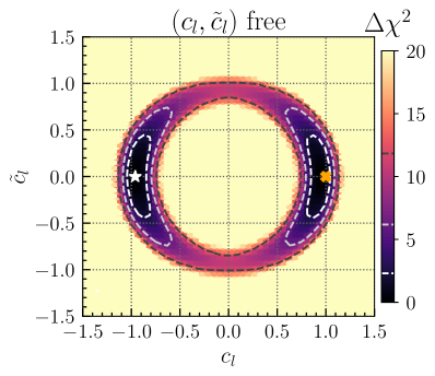
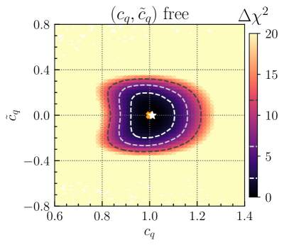
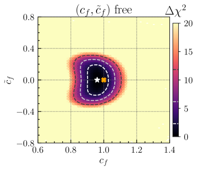
Figure 6: Results of fits to the LHC measurements in the (a) ($c_{l}$, $\tilde{c}_{l}$), (b) ($c_{q}$, $\tilde{c}_{q}$), and (c) ($c_{f}$, $\tilde{c}_{f}$) parameter planes. In each case, the ${\cal CP}$-even and ${\cal CP}$-odd parts of the couplings shown in the plot are free-floating while all the other parameters are set to their SM values. The legend corresponds to the one in Fig. 2.

4.1.3 Lepton, quark and fermion models

Next, we investigate models in which the Higgs couplings to leptons, quarks, or all fermions are modified simultaneously with the two coupling modifiers ($c_{l}$, $\tilde{c}_{l}$), ($c_{q}$, $\tilde{c}_{q}$) and ($c_{f}$, $\tilde{c}_{f}$), respectively. The results are shown in Fig. 6. In Fig. 6, where the lepton couplings $c_{l}$ and $\tilde{c}_{l}$ are varied, only the constraints provided by $H\to\tau^{+}\tau^{-}$ measurements play a significant role. Consequently, the results are very similar to the $(c_{\tau},\tilde{c}_{\tau})$ results presented in Fig. 2. When varying the quark couplings $c_{q}$ and $\tilde{c}_{q}$, see Fig. 6, the constraints are dominated by the limits on the third generation couplings. The form of the constraints qualitatively resembles the one of the 1-flavor top quark Yukawa fit shown in Fig. 3. As a consequence of simultaneously varying the bottom Yukawa coupling and the respective effect on the $H\to b\bar{b}$ decay rate, the constraints are somewhat tighter in comparison to Fig. 3. We obtain very similar results if not only the quark couplings are varied simultaneously, but all Higgs–fermion couplings, see Fig. 6. In comparison to Fig. 6, the additionally relevant constraints originate from $H\to\tau^{+}\tau^{-}$ and change the exclusion boundaries only slightly. The best-fit points for the three discussed models are found at $\chi^{2}_{\rm{min}}$-values of 87.87, 89.20 and 88.26, respectively.

4.1.4 Universal and fermion+V models

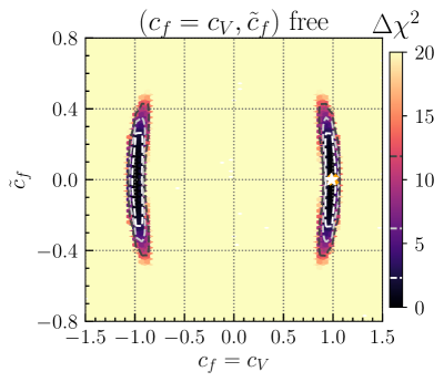
Figure 7: Results of fits to the LHC measurements in the ($c_{f}$, $\tilde{c}_{f}$) parameter plane with (a) $c_{f}=c_{V}$ and (b) $c_{V}$ free-floating. In each case, the ${\cal CP}$-even and ${\cal CP}$-odd parts of the couplings shown in the plot are free-floating while all the other parameters are set to their SM values. The legend corresponds to the one in Fig. 2.

We now consider the case where, as in Fig. 6, all Higgs–fermion couplings are varied simultaneously by the two parameters $c_{f}$ and $c_{f}$, but in addition $c_{f}=c_{V}$ holds, see Fig. 7, or $c_{V}$ is free-floating, see Fig. 7. In the scenario with $c_{f}=c_{V}$, measurements sensitive to the Higgs coupling to massive vector bosons (e.g. of $H\to WW^{*},ZZ^{*}$ or Higgs boson production via vector boson fusion) constrain $c_{V}$ and therefore also have an impact on $c_{f}$. On the other hand, only the $H\to\gamma\gamma$ decay (as well as $tH$ and $tWH$ production, for details see Bahl:2020wee) have a significant dependence on the sign of the ${\cal CP}$-even Higgs–fermion couplings (i.e. on the sign of $c_{t}$). This dependence is proportional to $c_{V}c_{t}$. As a consequence, the preference for a positive sign of $c_{t}$ vanishes if $c_{V}$ is allowed to have negative values. Accordingly, in the fit for the case $c_{f}=c_{V}$ shown in Fig. 7 the preferred region for $c_{f}$ is found close to $\pm 1$. If instead $c_{V}$ is floated independently, see Fig. 7, the result is qualitatively similar. As a consequence of the free-floating $c_{V}$, the constraints are somewhat weaker than in Fig. 7. The best-fit point in the two models with $c_{f}=c_{V}$ or free-floating $c_{V}$ has $\chi^{2}_{\rm{min}}$ = 88.40 and $\chi^{2}_{\rm{min}}$ = 87.97, respectively.

4.1.5 Fermion-vector and up-down-lepton-vector models

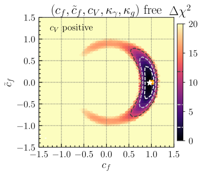
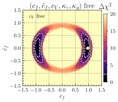
Figure 8: Results of fits to the LHC measurements in the ($c_{f}$, $\tilde{c}_{f}$) parameter plane. The coupling modifiers $c_{f}$, $\tilde{c}_{f}$, $\kappa_{\gamma}$, $\kappa_{g}$ are free-floating in both plots, while (a) $c_{V}$ is restricted to positive values and (b) $c_{V}$ is free-floating. In each case, the ${\cal CP}$-even and ${\cal CP}$-odd parts of the couplings shown in the plot are free-floating while all the other parameters are set to their SM values. The legend corresponds to the one in Fig. 2.

So far, we have treated the effective Higgs couplings to gluons and photons ($\kappa_{g}$ and $\kappa_{\gamma}$) as dependent parameters using Eqs. 5 and 6. We can, however, also treat them as free parameters, thus allowing for possible effects of unknown colored or charged BSM particles. This case is studied in Fig. 8, in which $c_{f}$, $\tilde{c}_{f}$, $c_{V}$, $\kappa_{g}$, and $\kappa_{\gamma}$ are floated freely. If $c_{V}$ is restricted to be positive, see Fig. 8, we expect in principle a similar result as obtained in Bahl:2020wee, where $c_{t}$, $\tilde{c}_{t}$, $c_{V}$, $\kappa_{g}$, and $\kappa_{\gamma}$ were floated (assuming $c_{V}$ to be positive). The CMS $H\to\tau^{+}\tau^{-}$ ${\cal CP}$ analysis, however, leads to additional constraints limiting $|\tilde{c}_{f}|\lesssim 0.37$ at the $1\,\sigma$ level, while in Bahl:2020wee a range of $\sim[-1.1,1.1]$ was found for $\tilde{c}_{t}$. If we allow $c_{V}$ to be negative, see Fig. 8, also negative $c_{f}$ values are allowed (see the discussion of Fig. 7). The best-fit point corresponds to $\chi^{2}_{\rm{min}}$ = 87.94 in both cases.

4.2 Impact of EDM and BAU constraints

In this Section, we will investigate the impact of the eEDM constraint by employing the ACME result [54] (see Section 3.2). Additionally, the amount of the BAU that can be reached based on the (optimistic) VIA approach for the displayed parameter regions will be indicated in the plots. As discussed in Section 3.3, we treat parameter regions with $Y_{B}^{\text{VIA}}/Y_{B}^{\text{obs}}\geq 1$ as favored by baryogenesis.

The LHC constraints will be applied at the 90% CL in this section in order to treat them at the same level as the eEDM constraint whose 90% CL cannot be translated into a 95% CL bound without further information. Regions in the parameter space that are within the limits from the LHC and ACME measurements at the $90\%$ CL and for which $Y_{B}^{\text{VIA}}/Y_{B}^{\text{obs}}\geq 1$ holds are colored in green.

4.2.1 1-flavor models

We first investigate models in which only the Higgs couplings to one fermion species are allowed to float freely. The same fermions as in Sec. 4.1.1 will be considered. Contributions from the individual coupling modifiers on the total predicted values for eEDM and BAU are calculated according to the formulas given in Eqs. 13 and 15, where the Higgs–electron coupling is assumed to be SM-like ($c_{e}=1$, $\tilde{c}_{e}=0$). The case where this assumption on the Higgs–electron coupling is relaxed will be discussed in Sec. 4.2.4.

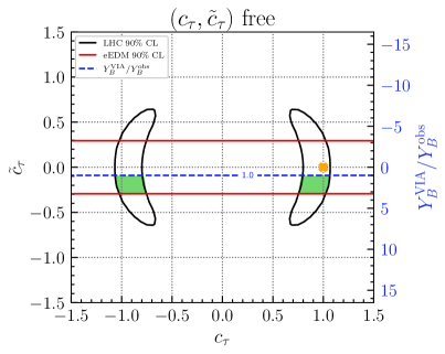
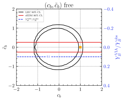
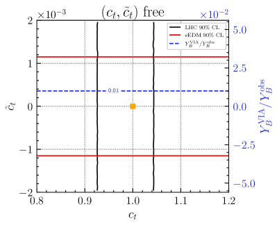
Figure 9: Constraints on the ${\cal CP}$-even and ${\cal CP}$-odd modifiers of (a) the tau-Yukawa, (b) the bottom-Yukawa, as well as (c) the top-Yukawa interactions based on LHC measurements (black), eEDM limits (red), and the ratio $Y_{B}^{\text{VIA}}/Y_{B}^{\text{obs}}$ (blue contours and vertical scale on the right). The green colored areas indicate the parameter regions satisfying the LHC and eEDM constraints for which $Y_{B}^{\text{VIA}}/Y_{B}^{\text{obs}}\geq 1$.

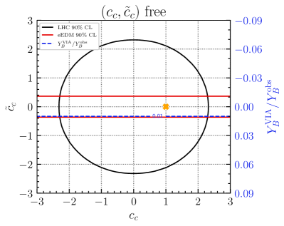
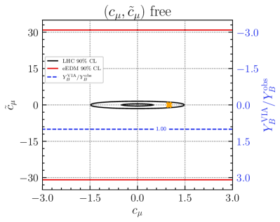
Figure 10: Constraints on the ${\cal CP}$-even and ${\cal CP}$-odd modifiers of (a) the charm-Yukawa as well as (b) the muon-Yukawa interactions. The legend corresponds to the one in Fig. 9.

Our results are presented in Figs. 9 and 10. The eEDM contour lines (red) show where the measured upper limit of ACME is reached. The amount of BAU that can be reached, see Eq. 15, is indicated in the plots as a second axis on the right with an additional blue dashed horizontal line at specific values of $Y_{B}^{\text{VIA}}/Y_{B}^{\text{obs}}$ for illustration. Like the eEDM, it only depends on the respective ${\cal CP}$-odd coupling modifiers. Negative $Y_{B}^{\text{VIA}}/Y_{B}^{\text{obs}}$ values imply that more anti-baryons than baryons would have been produced in the early universe and are therefore strongly disfavored.

$\tau$ Yukawa coupling

In the model with free-floating tau Yukawa couplings as in Sec. 4.1, see Fig. 9, constraints on $c_{\tau}$ arise mainly due to the CMS $H\to\tau^{+}\tau^{-}$ ${\cal CP}$ analysis. The strongest constraint on $\tilde{c}_{\tau}$, on the other hand, is the eEDM measurement, limiting $|\tilde{c}_{\tau}|\lesssim 0.29$ at the 90% CL. This directly translates into $Y_{B}^{\text{VIA}}/Y_{B}^{\text{obs}}\lesssim 3.2$, meaning that ${\cal CP}$ violation in the Higgs–tau coupling alone would be sufficient to explain the observed BAU, based on the (optimistic) VIA approach.

$b$ Yukawa coupling

Similarly, $\tilde{c}_{b}$ is also predominantly constrained by the eEDM, see Fig. 9. As a consequence of the smaller contribution of $\tilde{c}_{b}$ to the baryon asymmetry, however, $Y_{B}^{\text{VIA}}/Y_{B}^{\text{obs}}$ is limited to be $\lesssim 0.05$ within the parameter region that is allowed by the eEDM and LHC constraints. For illustration, we have indicated the line with $Y_{B}^{\text{VIA}}/Y_{B}^{\text{obs}}=0.1$, which lies outside of the region that is allowed by the eEDM constraint.

$t$ Yukawa coupling

The eEDM measurement has an even stronger impact on $\tilde{c}_{t}$, as can be seen in Fig. 9. We scale the vertical axis by a factor of $10^{-3}$ in this panel in order to make the eEDM constraint visible. Note, however, that the eEDM constraint strongly depends on the electron Yukawa coupling — as will be investigated below —, which here is assumed to be SM-like. As a consequence of the rescaled vertical axis, constraints from the LHC appear as straight lines. The realizable amount of BAU in a scenario where just the Higgs–top coupling deviates from the SM is therefore very small. Within the region that is allowed by the eEDM constraint we find $Y_{B}^{\text{VIA}}/Y_{B}^{\text{obs}}\lesssim 0.033$.

$c$ Yukawa coupling

Floating the charm quark Yukawa coupling modifiers (see Fig. 10), we observe that the eEDM measurement imposes the dominant constraint on the respective ${\cal CP}$-odd coupling, as it was the case for the third-generation fermion couplings. Within the parameter region that is allowed by the eEDM constraint, only $Y_{B}^{\text{VIA}}/Y_{B}^{\text{obs}}\lesssim 0.01$ can be reached.

$\mu$ Yukawa coupling

For the case where the Yukawa coupling of the muon is allowed to float, see Fig. 10, we find qualitatively different results. Due to the small muon Yukawa coupling, the eEDM constraint on $\tilde{c}_{\mu}$ is weak, allowing for $\tilde{c}_{\mu}<31$ which corresponds to $Y_{B}^{\text{VIA}}/Y_{B}^{\text{obs}}\lesssim 3.1$. However, the measurement of the $H\to\mu^{+}\mu^{-}$ decay at the LHC outperforms the eEDM by constraining the imaginary part of the muon Yukawa coupling to maximally $\tilde{c}_{\mu}<1.6$ (for $c_{\mu}=0$), corresponding to $Y_{B}^{\text{VIA}}/Y_{B}^{\text{obs}}\lesssim 0.16$. Hence, the sensitivity to this rare decay already provides the dominant information on the ${\cal CP}$-odd part of the muon Yukawa coupling, in agreement with the findings of Ref. [62].

4.2.2 2-flavor models

In Figs. 11 and 12 we consider modifications of the Higgs interactions with two different flavors.

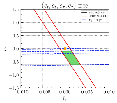
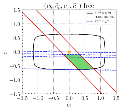
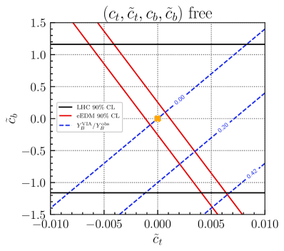
Figure 11: Constraints on the ${\cal CP}$-odd modifiers of (a) the top- and tau-, (b) the bottom- and tau-, as well as (c) the top- and bottom-Yukawa interactions based on LHC measurements (black), eEDM limits (red), and the ratio $Y_{B}^{\text{VIA}}/Y_{B}^{\text{obs}}$ (blue). For the LHC constraints, the corresponding ${\cal CP}$-even modifiers are profiled. The legend corresponds to the one in Fig. 9.

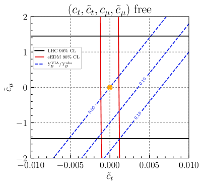
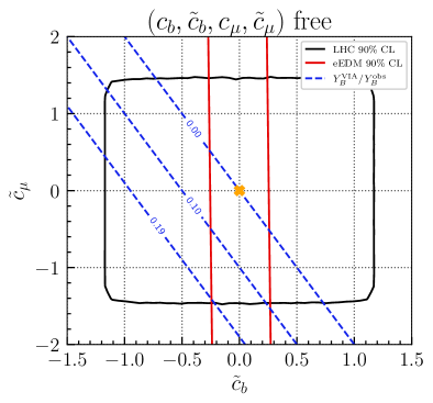
Figure 12: Constraints on the ${\cal CP}$-odd modifiers of (a) the top- and muon-, as well as (b) the bottom- and muon-Yukawa interactions. The legend corresponds to the one in Fig. 9.

$\boldsymbol{t+\tau}$ Yukawa couplings

In Fig. 11, we investigate the possibility of ${\cal CP}$ violation in the top quark and tau Yukawa couplings. Since a sufficient amount of ${\cal CP}$ violation to explain the BAU (in the VIA approach) can already be generated from the tau Yukawa coupling alone, see Fig. 9, it can also be achieved when combining a free tau Yukawa coupling with an additional source of ${\cal CP}$ violation. The effects of complex tau and top quark Yukawa couplings can cancel each other in the prediction for the eEDM resulting in the diagonal red eEDM contours. Hence, larger values of $Y_{B}^{\text{VIA}}/Y_{B}^{\text{obs}}\lesssim 6.9$ are accessible as compared to the case where only the couplings of one fermion flavor are allowed to float.

$\boldsymbol{b+\tau}$ Yukawa couplings

A very similar behavior is observed when allowing for ${\cal CP}$ violation in the bottom quark and tau Yukawa couplings, with $Y_{B}^{\text{VIA}}/Y_{B}^{\text{obs}}$ again reaching maximally 6.9, as shown in Fig. 11. Since the overall contribution of $\tilde{c}_{b}$ to the eEDM is smaller, larger values of $|\tilde{c}_{b}|$ are possible in comparison to the allowed $|\tilde{c}_{t}|$ values in Fig. 11.

$\boldsymbol{t+b}$ Yukawa couplings

The possibility of ${\cal CP}$ violation in the bottom quark and top quark Yukawa interactions is investigated in Fig. 11. While in the 1-flavor case $\tilde{c}_{b}$ ($\tilde{c}_{t}$) can only reach a small fraction of the observed BAU, $Y_{B}^{\text{VIA}}/Y_{B}^{\text{obs}}=0.05~{}(0.03)$, their combination can amount for up to $Y_{B}^{\text{VIA}}/Y_{B}^{\text{obs}}=0.42$ within the LHC and eEDM limits due to large cancellations in the eEDM prediction. Although this remains short of the full baryon asymmetry, the contribution arising from the combination of the couplings is several times larger than the sum of the individual contributions. This is a qualitatively different result compared to Fig. 5 of Fuchs:2020uoc, where the maximal value of $Y_{B}^{\text{VIA}}/Y_{B}^{\text{obs}}$ was found to be 0.12. The larger $Y_{B}^{\text{VIA}}/Y_{B}^{\text{obs}}$ value determined here is a consequence of profiling over $c_{b}$ and $c_{t}$ instead of fixing $c_{t}=c_{b}=1$ as done in Fuchs:2020uoc.

$\boldsymbol{t+\mu},~{}\boldsymbol{b+\mu}$ Yukawa couplings

When allowing for ${\cal CP}$ violation in the top quark and muon Yukawa interactions, see Fig. 12, or in the bottom quark and muon Yukawa interactions, see Fig. 12, no sufficient amount of ${\cal CP}$ violation can be generated while satisfying the LHC and eEDM constraints — the maximal reachable $Y_{B}^{\text{VIA}}/Y_{B}^{\text{obs}}$ values are $\sim 0.18$ and $\sim 0.19$, respectively, i.e. just a small increase compared to the contribution of the muon alone.

4.2.3 Fermion and fermion+V models

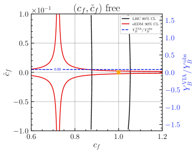
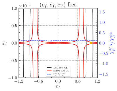
Figure 13: Constraints on the global Higgs–fermion coupling modifiers $c_{f}$ and $\tilde{c}_{f}$ where $c_{V}$ is (a) set to its SM value or (b) free-floating in the fit. The legend corresponds to the one in Fig. 9.

Instead of varying the coupling modifiers of one or two Higgs–fermion interactions, we now consider the case where all Higgs–fermion coupling modifiers are varied in the same way by floating the global modifiers $c_{f}$ and $\tilde{c}_{f}$, see Fig. 13. In this scenario, the coupling modifiers are varied simultaneously for the top quark Yukawa and the electron Yukawa coupling, which can potentially give rise to cancellations of the different contributions in the eEDM calculation. Indeed, the star-like shape of the contour of the eEDM constraint arises from a cancellation for $c_{f}\approx 0.73$, for which sizable contributions of $|\tilde{c}_{f}|\gtrsim 0.1$ are allowed. The collider bounds in Fig. 13 correspond to the ones shown in Fig. 6. Since the region with significant cancellations in the eEDM prediction has only a small overlap with the region that is allowed by the LHC constraint, the reachable $Y_{B}^{\text{VIA}}/Y_{B}^{\text{obs}}$ values are only slightly increased to $0.08$ as compared to a single flavor modification of the top quark or bottom quark Yukawa coupling.

In addition to varying $c_{f}$ and $\tilde{c}_{f}$, also $c_{V}$ is free-floated in Fig. 13. For the eEDM calculation, we vary $c_{V}$ within its 90% CL LHC limits and then derive the minimal possible $|d_{e}|$ value. Similarly to Fig. 13, the eEDM constraint gives rise to a star-like shaped contour. Since the relative size of $c_{f}$ and $c_{V}$ determines the position of this contour, see Eq. 13, floating $c_{V}$ results in a second star-like allowed eEDM region for negative values of $c_{f}$. Furthermore, floating $c_{V}$ gives rise to a smearing of the star shape in the $c_{f}$ direction. In comparison to Fig. 13, the reachable $Y_{B}^{\text{VIA}}/Y_{B}^{\text{obs}}$ values are slightly increased to 0.11.

4.2.4 Top and electron Yukawa couplings

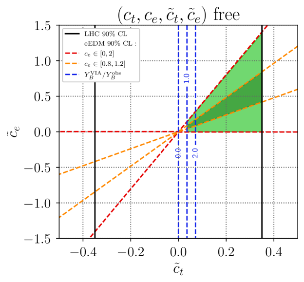
Figure 14: Constraints on the ${\cal CP}$-odd modifiers of the top- and electron-Yukawa interactions with the legend similar to Fig. 9. For evaluating the eEDM, $c_{t}$ is varied within its $90\%$ CL collider limits, and $c_{e}$ is varied in the interval $[0,2]$ (red contours) and $[0.8,1.2]$ (orange contours).

As discussed above, the eEDM sets strong constraints on ${\cal CP}$ violation in the Higgs sector, in particular for the top quark Yukawa interaction, if the electron Yukawa coupling is close to its SM value. However, these constraints may vary a lot depending on the value of the electron-Yukawa coupling, which is only very weakly constrained by LHC measurements. In the extreme case of a zero electron Yukawa coupling (i.e. $c_{e}=\tilde{c}_{e}=0$), the prediction for the eEDM would be strongly suppressed regardless of the amount of ${\cal CP}$ violation in other Higgs couplings. But even in the case of only a small deviation in the electron-Yukawa coupling from the SM value, large cancellations can occur in the eEDM prediction between the contributions involving the components of the top quark and the electron Yukawa couplings.

This is illustrated in Fig. 14, showing the LHC and eEDM constraints on a model in which the coupling modifiers of the electron and top quark Yukawa interactions are floated freely. The results are depicted in the $(\tilde{c}_{t},\tilde{c}_{e})$ parameter plane. Since the LHC limits on the electron Yukawa coupling are not relevant in the displayed parameter space, the LHC constraints appear as vertical lines limiting $\tilde{c}_{t}$ to be within $\sim[-0.35,0.35]$ at the 90% CL (for the LHC constraints we profile over $c_{t}$). Varying the electron Yukawa coupling modifiers, however, strongly affects the eEDM prediction. At every point in the $(\tilde{c}_{t},\tilde{c}_{e})$ parameter plane, we vary $c_{t}$ within its $90\%$ CL LHC limits and $c_{e}$ in the interval $[0,2]$ (red contours) or in the interval $[0.8,1.2]$ (orange contours); then, we derive the minimal possible $d_{e}$ value. Since the contribution of a ${\cal CP}$-violating electron Yukawa coupling enters with a coefficient of similar size as the contribution of a ${\cal CP}$-violating top quark Yukawa coupling, see Eq. 13, large cancellations can occur for appropriate values of $c_{e}$, $\tilde{c}_{e}$, $c_{t}$ and $\tilde{c}_{t}$. As a consequence, much larger $\tilde{c}_{t}$ values become accessible than in Fig. 9. As indicated by the different sizes of the regions enclosed by the red and orange contours, varying $c_{e}$ in a larger region would make an even larger portion of the shown parameter space compatible with the eEDM constraint. As long as $\tilde{c}_{e}$ floats freely, a sufficient amount of ${\cal CP}$ violation to explain the BAU can be generated (see the green colored regions), which corresponds to $Y_{B}^{\text{VIA}}/Y_{B}^{\text{obs}}\lesssim 9.8$. Note, however, that at sizeable values of $\tilde{c}_{t}$ or $\tilde{c}_{e}$ a large amount of fine-tuning is necessary for those cancellations to occur.

4.2.5 Comparison of the maximal contributions to the BAU

We summarize some of the results of this section in Table 2, where we list the maximal values for $Y_{B}^{\text{VIA}}/Y_{B}^{\text{obs}}$ that are obtained within the regions allowed by the LHC and eEDM constraints at 90% CL for all combinations of two out of the five considered fermion flavors, where either the modifiers for one or two couplings are varied. The modifiers for the electron Yukawa coupling in this table are fixed to $c_{e}=1$, $\tilde{c}_{e}=0$. The largest amount of $Y_{B}^{\text{VIA}}/Y_{B}^{\text{obs}}$ with a single ${\cal CP}$-violating Higgs–fermion coupling can be reached by allowing for ${\cal CP}$ violation in the tau Yukawa coupling. This feature of the tau Yukawa coupling is due to a combination of several reasons. First, leptons are not affected by the strong sphalerons that would wash out the initial asymmetry [175]. Moreover, the diffusion of the asymmetry across the bubble wall is more efficient for leptons [162, 176]. Finally, the smaller Yukawa coupling of the tau lepton compared to the top quark leads to a weaker bound from the eEDM.

Adding ${\cal CP}$ violation in a second Higgs–fermion coupling increases the reachable $Y_{B}^{\text{VIA}}/Y_{B}^{\text{obs}}$ by a factor of $\sim 2.2$. Allowing for ${\cal CP}$ violation only in up to two Higgs–fermion couplings excluding the tau and the electron Yukawa couplings, a sufficient amount of ${\cal CP}$ violation to explain the baryon asymmetry of the universe cannot be reached – not even in the optimistic VIA framework. The highest reachable value of $Y_{B}^{\text{VIA}}/Y_{B}^{\text{obs}}$ in this case is $\sim 0.42$, obtained by allowing for ${\cal CP}$ violation in the top quark and bottom quark Yukawa couplings. For the scenario with global Higgs-fermion coupling modifiers, we obtained a maximally reachable value of $Y_{B}^{\text{VIA}}/Y_{B}^{\text{obs}}\sim 0.08$. If in addition also $c_{V}$ is varied, a slightly higher value of $Y_{B}^{\text{VIA}}/Y_{B}^{\text{obs}}\sim 0.11$ can be reached.

	$t$	$b$	$c$	$\tau$	$\mu$
$t$	0.03
$b$	0.42	0.05
$c$	0.37	0.19	0.01
$\tau$	6.9	6.9	6.9	3.2
$\mu$	0.18	0.19	0.16	3.2	0.16

Table 2: Maximal values of $Y_{B}^{\text{VIA}}/Y_{B}^{\text{obs}}$ within the regions that are allowed by the LHC and eEDM constraints at 90% CL for all combinations of the five considered fermion flavors, where the modifiers of up to two couplings are varied. The electron-Yukawa coupling is fixed at $c_{e}=1$, $\tilde{c}_{e}=0$. The diagonal entries of the Table represent the cases where only one Yukawa coupling is modified.

5 Conclusions

${\cal CP}$ violation in Higgs–fermion interactions is an intriguing possibility, since it could play an important role in explaining the observed asymmetry between matter and antimatter in the universe. In this work, we have explored this option by taking into account inclusive and differential experimental results from LHC measurements of Higgs production and decay processes and the eEDM limit in combination with theoretical predictions in an effective model description. After determining the parameter space that is favored by these constraints, we have assessed to which extent ${\cal CP}$ violation in the Higgs–fermion couplings can contribute to the observed baryon asymmetry.

The first part of this work focused on the LHC constraints on ${\cal CP}$-violating Higgs–fermion couplings. The Higgs characterization model has been used, allowing not only a variation of the various Higgs–fermion couplings but also of the Higgs coupling to massive vector bosons as well as of the effective Higgs couplings to gluons and photons. Besides including total and differential rate measurements, we also included into our global fit the recent dedicated $H\to\tau^{+}\tau^{-}$ ${\cal CP}$ analysis performed by the CMS collaboration [15]. This yields $|\tilde{c}_{\tau}|<0.75$ at the 95% CL considering the scenario where only the components of the tau Yukawa coupling are allowed to float freely (1-flavor model), whereas $|\tilde{c}_{\tau}|<1.1$ would have been allowed if only the ${\cal CP}$-conserving rate measurements had been taken into account.

We studied the LHC constraints by investigating models with increased complexity. The simplest cases are the 1-flavor models, in which we allowed for deviations from the SM in the interaction of the Higgs boson with only one fermion species. Here, we found the strongest constraints for ${\cal CP}$-violating tau and top quark Yukawa couplings, where the latter is mainly constrained by Higgs production and the decay into photons (for the constraints on the tau Yukawa coupling see the discussion above). On the other hand, the LHC constraints on the ${\cal CP}$-violating bottom quark and muon Yukawa couplings are currently driven by the ${\cal CP}$ conserving observables from the Higgs decay into these fermions. In contrast, the complex charm quark Yukawa coupling is most stringently constrained by the precise measurement of the $H\to\gamma\gamma$ decay rate via the modification of the total Higgs width. These constraints from Higgs decays give rise to rings of allowed parameters in the plane of the modifiers of the real and imaginary parts of the couplings. The first generation Yukawa couplings are still almost unconstrained.

When allowing for ${\cal CP}$ violation in the Higgs interactions with two fermion species, we found the LHC constraints on the different species to be only weakly correlated, so that the constraints from the 1-flavor modification fits were largely recovered. As an alternative approach, we studied models in which the couplings of a specific group of fermions are modified universally (e.g. of all quarks or all leptons). As expected, we found the constraints on the third generation couplings to always dominate the fit results with the top quark Yukawa constraints being the most important among these. We extended these fit results by increasing the number of coupling modifiers that are allowed to float independently of each other to up to nine (see the discussion in Appendix A). Generally, our fit confirms the expectation that the allowed parameter region is enlarged in models with additional freedom.

As complementary constraints, we then studied the impact of the eEDM bound and assessed to which extent the BAU can be explained within the parameter regions that are in agreement with the LHC and eEDM constraints. Our approach in this context accounts for the fact that the BAU predictions are affected by large theoretical uncertainties that are in particular related to the choice made in the calculation framework regarding the use of the VIA or the WKB approach [170]. We therefore did not require in our analysis that the BAU prediction using the VIA has to match the observed value, but we have treated all values of $Y_{B}^{\text{VIA}}/Y_{B}^{\text{obs}}\geq 1$ as theoretically allowed. Since the results for the BAU obtained via the WKB approach are significantly smaller than the ones based on the VIA, even for $Y_{B}^{\text{VIA}}/Y_{B}^{\text{obs}}\geq 1$ further sources of ${\cal CP}$ violation besides the couplings of the observed Higgs signal at $125\,\,\mathrm{GeV}$ might be needed. On the other hand, we regard parameter regions with $Y_{B}^{\text{VIA}}/Y_{B}^{\text{obs}}<1$ as disfavored by the observed BAU because the bubble wall parameters used in the VIA calculation are near the values that maximize the predicted BAU.

Using this approach, we found that the amount of ${\cal CP}$ violation in the tau Yukawa coupling that is allowed by the latest LHC and eEDM constraints would suffice to explain the BAU (if calculated in the VIA framework) even if it occurs as the only source of ${\cal CP}$ violation in addition to the CKM phase. While similar conclusions were drawn previously, see Guo:2016ixx,DeVries:2018aul,Fuchs:2020uoc,Shapira:2021mmy, we reevaluated this statement based on a non-trivial global fit taking into account the very significantly improved constraints on the imaginary part of the tau Yukawa coupling that arise in particular from the inclusion of the recent angular analysis performed by the CMS Collaboration. Still, the eEDM remains the strongest bound on $\tilde{c}_{\tau}$, yielding $\tilde{c}_{\tau}$ <0.3 at the 90% CL in the 1-flavor case, i.e. about a factor of 2 stronger than the angular CMS analysis. Moreover, we have confirmed that the feature that ${\cal CP}$ violation in the tau Yukawa coupling could account for the whole BAU is unique to this coupling. Our results show that this is not possible for ${\cal CP}$ violation in any other single Yukawa coupling and it also cannot be realized for the case where ${\cal CP}$ violation in two other third- or second-generation Yukawa couplings (i.e. excluding the tau Yukawa coupling) is allowed.

Regarding the eEDM, it should be noted that the impact of this constraint crucially depends on the chosen input value for the electron Yukawa coupling, which is still almost completely unconstrained by LHC measurements. Treating this unknown quantity as a free parameter reduces the contributions to the eEDM for the case where $|c_{e}|$ is below the SM value and gives rise to possible cancellations between the different contributions to the eEDM for the case of ${\cal CP}$ violation in the electron Yukawa coupling. Accordingly, in those cases substantial parts of the considered parameter space are phenomenologically viable even in view of the latest improvement of the eEDM limit.

Our analysis has demonstrated that the analysis of possible ${\cal CP}$ violation in the Higgs sector is of particular interest, since ${\cal CP}$-violating Yukawa couplings can potentially explain the BAU while satisfying all relevant experimental and theoretical constraints. The further exploration of this issue will greatly profit from the complementarity between the information obtainable at colliders, from the EDMs of the electron and of other systems, as well as from improvements in the predictions for the BAU.

Appendix A Additional fit results

In this Appendix, we collect our results of additional fits to LHC data which are supplementary to the results presented in Section 4.

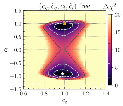
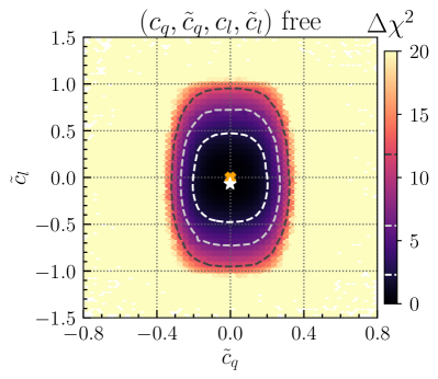
Figure 15: Results of fits to the LHC measurements in the (a) ($c_{q}$, $c_{l}$) and (b) ($\tilde{c}_{q}$, $\tilde{c}_{l}$) parameter plane. In both cases, the four parameters shown in the plot are free-floating while all the other parameters are set to their SM values. The legend corresponds to the one in Fig. 2.

Quark–lepton model

One possibility that was not explored in Section 4 is to allow for separate modifications in the quark and lepton sector (varying $c_{q}$, $\tilde{c}_{q}$, $c_{l}$, and $\tilde{c}_{l}$). The corresponding fit results are shown in Fig. 15. The results are similar to the two-flavor fit in which $c_{t}$, $\tilde{c}_{t}$, $c_{\tau}$, and $\tilde{c}_{\tau}$ are varied (see Figs. 5 and 5), with $\chi^{2}_{\rm{min}}$ = 87.84. The quark and lepton sectors are again only weakly correlated via the $H\to\gamma\gamma$ decay process. Setting $c_{b}=c_{t}\equiv c_{q}$ and $\tilde{c}_{b}=\tilde{c}_{t}\equiv\tilde{c}_{q}$ slightly tightens the constraints in comparison to Figs. 5 and 5.

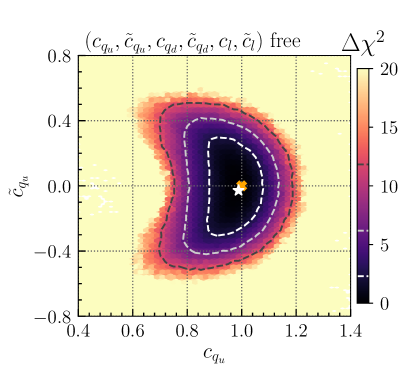
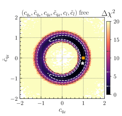
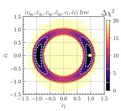
Figure 16: Results of fits to the LHC measurements in the (a) ($c_{q_{u}}$, $\tilde{c}_{q_{u}}$), (b) ($c_{q_{d}}$, $\tilde{c}_{q_{d}}$), and (c) ($c_{l}$, $\tilde{c}_{l}$) parameter plane. For each plot the indicated coupling modifiers are free-floating while all the other parameters are set to their SM values. The legend corresponds to the one in Fig. 2.

Up–down–lepton model

The results can be further generalized by treating the up- and down-type quark sector separately. The fit results of varying $c_{q_{u}}$, $\tilde{c}_{q_{u}}$, $c_{q_{d}}$, $\tilde{c}_{q_{d}}$, $c_{l}$, and $\tilde{c}_{l}$ are shown in Fig. 16. The constraints on the different sectors are again dominated by the constraints on the third generation couplings and only weakly correlated: the constraints on $c_{q_{u}}$ and $\tilde{c}_{q_{u}}$, see Fig. 16, resemble the $(c_{t},\tilde{c}_{t})$ fit shown in Fig. 3 with the bounds being slightly looser due to the additional variation of the bottom-Yukawa coupling; the constraints on $c_{q_{d}}$ and $\tilde{c}_{q_{d}}$, see Fig. 16, resemble the $(c_{b},\tilde{c}_{b})$ fit shown in Fig. 3 with the bounds being slightly looser due to the additional variation of the top-Yukawa coupling; the constraints on $c_{l}$ and $\tilde{c}_{l}$, see Fig. 16, resemble the $(c_{l},\tilde{c}_{l})$ fit shown in Fig. 6. The best-fit point is found at $\chi^{2}_{\rm{min}}$ = 87.80.

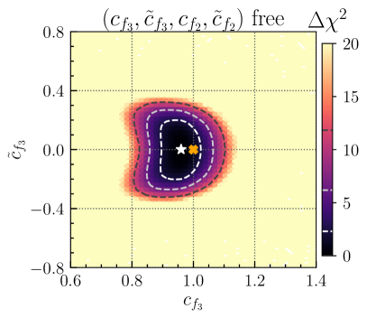
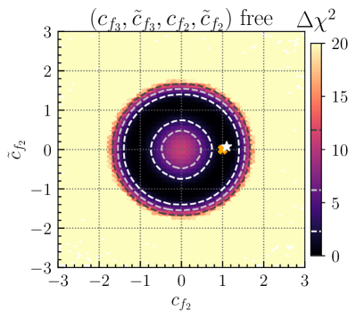
Figure 17: Results of fits to the LHC measurements in the (a) ($c_{f_{3}}$, $\tilde{c}_{f_{3}}$) and (b) ($c_{f_{2}}$, $\tilde{c}_{f_{2}}$) parameter plane. For each plot the indicated coupling modifiers are free-floating while all the other parameters are set to their SM values. The legend corresponds to the one in Fig. 2.

2${}^{\text{nd}}$/3${}^{\text{rd}}$ generation model

Another possibility to generalize the fit results is to differentiate the second and third generation (we do not refer to the first generation here, since the collider limits on the first generation obtained so far are very weak). The corresponding fit results floating $c_{f_{3}}$, $\tilde{c}_{f_{3}}$, $c_{f_{2}}$, and $\tilde{c}_{f_{2}}$ are shown in Fig. 17. There is hardly any correlation between the constraints on the second and third generation. Therefore, the constraints on the third generation, see Fig. 17, are very similar to the $(c_{f},\tilde{c}_{f})$ fit presented in Fig. 6. The constraints on the second generation, shown in Fig. 17, are dominated by the constraints on the muon-Yukawa coupling (see Fig. 3). The best-fit point has $\chi^{2}_{\rm{min}}$ = 87.68.

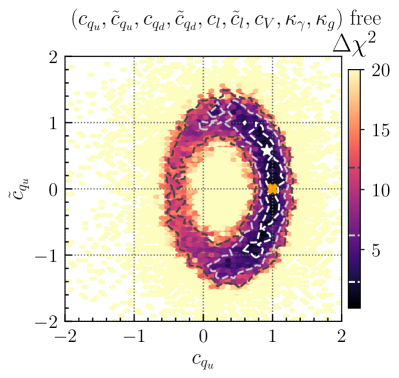
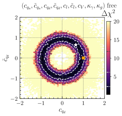
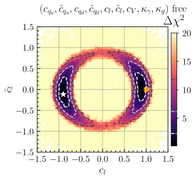
Figure 18: Results of fits to the LHC measurements in the (a) ($c_{q_{u}}$, $\tilde{c}_{q_{u}}$), (b) ($c_{q_{d}}$, $\tilde{c}_{q_{d}}$), and (c) ($c_{l}$, $\tilde{c}_{l}$) parameter plane. All parameters listed above the plot panels are floated freely. The legend corresponds to the one in Fig. 2.

Up–down–lepton–vector model

As the most general model considered in this work, we do not only vary the up-, down-, and lepton-Yukawa couplings separately, but in addition we also freely float $c_{V}$, $\kappa_{g}$, and $\kappa_{\gamma}$. The resulting constraints in the $(c_{q_{u}},\tilde{c}_{q_{u}})$, $(c_{q_{d}},\tilde{c}_{q_{d}})$, and $(c_{l},\tilde{c}_{l})$ parameter planes are shown in Fig. 18, with $\chi^{2}_{\rm{min}}$ = 87.80. In Fig. 18, showing the constraints for the up-type Yukawa couplings, we observe a significantly enlarged allowed region in comparison to Fig. 16. This is mainly a consequence of freely floating $\kappa_{g}$ and $\kappa_{\gamma}$ (for a more detailed discussion see Bahl:2020wee). The constraints on the down-type Yukawa couplings, see Fig. 18, are only slightly weaker in comparison to Fig. 16. As a consequence of freely floating $\kappa_{g}$, $c_{q_{d}}\simeq-1$ is allowed at the one-sigma level. For the constraints on the lepton-Yukawa couplings, see Fig. 18, the boundaries of the $3\,\sigma$ region are slightly tighter than in Fig. 16. This is most likely an artefact of the coarse sampling, which could be avoided with an increased sample size.

References

- [1] G. Aad “Observation of a new particle in the search for the Standard Model Higgs boson with the ATLAS detector at the LHC” In Phys. Lett. B716, 2012, pp. 1–29 DOI: 10.1016/j.physletb.2012.08.020
- [2] S. Chatrchyan “Observation of a new boson at a mass of 125 GeV with the CMS experiment at the LHC” In Phys. Lett. B716, 2012, pp. 30–61 DOI: 10.1016/j.physletb.2012.08.021
- [3] Georges Aad “Measurements of the Higgs boson production and decay rates and constraints on its couplings from a combined ATLAS and CMS analysis of the LHC pp collision data at and 8 TeV” In JHEP 08, 2016, pp. 045 DOI: 10.1007/JHEP08(2016)045
- [4] Georges Aad “Combined measurements of Higgs boson production and decay using up to fb-1 of proton-proton collision data at 13 TeV collected with the ATLAS experiment” In Phys. Rev. D 101.1, 2020, pp. 012002 DOI: 10.1103/PhysRevD.101.012002
- [5] Albert M Sirunyan “Combined measurements of Higgs boson couplings in proton–proton collisions at ” In Eur. Phys. J. C 79.5, 2019, pp. 421 DOI: 10.1140/epjc/s10052-019-6909-y
- [6] Vardan Khachatryan “Constraints on the spin-parity and anomalous HVV couplings of the Higgs boson in proton collisions at 7 and 8 TeV” In Phys. Rev. D 92.1, 2015, pp. 012004 DOI: 10.1103/PhysRevD.92.012004
- [7] Georges Aad “Study of the spin and parity of the Higgs boson in diboson decays with the ATLAS detector” [Erratum: Eur.Phys.J.C 76, 152 (2016)] In Eur. Phys. J. C 75.10, 2015, pp. 476 DOI: 10.1140/epjc/s10052-015-3685-1
- [8] Georges Aad “Test of CP Invariance in vector-boson fusion production of the Higgs boson using the Optimal Observable method in the ditau decay channel with the ATLAS detector” In Eur. Phys. J. C 76.12, 2016, pp. 658 DOI: 10.1140/epjc/s10052-016-4499-5
- [9] Georges Aad “Test of CP invariance in vector-boson fusion production of the Higgs boson in the channel in protonproton collisions at = 13 TeV with the ATLAS detector” In Phys. Lett. B 805, 2020, pp. 135426 DOI: 10.1016/j.physletb.2020.135426
- [10] Albert M Sirunyan “Constraints on anomalous Higgs boson couplings using production and decay information in the four-lepton final state” In Phys. Lett. B 775, 2017, pp. 1–24 DOI: 10.1016/j.physletb.2017.10.021
- [11] Albert M Sirunyan “Constraints on anomalous couplings from the production of Higgs bosons decaying to lepton pairs” In Phys. Rev. D 100.11, 2019, pp. 112002 DOI: 10.1103/PhysRevD.100.112002
- [12] Albert M Sirunyan “Measurements of the Higgs boson width and anomalous couplings from on-shell and off-shell production in the four-lepton final state” In Phys. Rev. D 99.11, 2019, pp. 112003 DOI: 10.1103/PhysRevD.99.112003
- [13] dummy “Constraints on anomalous Higgs boson couplings to vector bosons and fermions in production and decay in the channel”, 2020
- [14] dummy “Constraints on Higgs boson properties using production in of pp collisions with the ATLAS detector”, 2020
- [15] Armen Tumasyan “Analysis of the CP structure of the Yukawa coupling between the Higgs boson and leptons in proton-proton collisions at = 13 TeV”, 2021 arXiv:2110.04836 [hep-ex]
- [16] B. Grzadkowski and J.. Gunion “Using decay angle correlations to detect CP violation in the neutral Higgs sector” In Phys. Lett. B 350, 1995, pp. 218–224 DOI: 10.1016/0370-2693(95)00369-V
- [17] Stefan Berge and Werner Bernreuther “Determining the CP parity of Higgs bosons at the LHC in the tau to 1-prong decay channels” In Phys. Lett. B 671, 2009, pp. 470–476 DOI: 10.1016/j.physletb.2008.12.065
- [18] Roni Harnik et al. “Measuring CP Violation in at Colliders” In Phys. Rev. D 88.7, 2013, pp. 076009 DOI: 10.1103/PhysRevD.88.076009
- [19] Albert M Sirunyan “Measurements of H production and the CP structure of the Yukawa interaction between the Higgs boson and top quark in the diphoton decay channel”, 2020 arXiv:2003.10866 [hep-ex]
- [20] Georges Aad “Study of the CP properties of the interaction of the Higgs boson with top quarks using top quark associated production of the Higgs boson and its decay into two photons with the ATLAS detector at the LHC”, 2020 arXiv:2004.04545 [hep-ex]
- [21] Albert M Sirunyan “Constraints on anomalous Higgs boson couplings to vector bosons and fermions in its production and decay using the four-lepton final state”, 2021 arXiv:2104.12152 [hep-ex]
- [22] Ayres Freitas and Pedro Schwaller “Higgs CP Properties From Early LHC Data” In Phys. Rev. D87.5, 2013, pp. 055014 DOI: 10.1103/PhysRevD.87.055014
- [23] Abdelhak Djouadi and Grégory Moreau “The couplings of the Higgs boson and its CP properties from fits of the signal strengths and their ratios at the 7+8 TeV LHC” In Eur. Phys. J. C73.9, 2013, pp. 2512 DOI: 10.1140/epjc/s10052-013-2512-9
- [24] John Ellis, Dae Sung Hwang, Kazuki Sakurai and Michihisa Takeuchi “Disentangling Higgs-Top Couplings in Associated Production” In JHEP 04, 2014, pp. 004 DOI: 10.1007/JHEP04(2014)004
- [25] Fawzi Boudjema, Rohini M. Godbole, Diego Guadagnoli and Kirtimaan A. Mohan “Lab-frame observables for probing the top-Higgs interaction” In Phys. Rev. D92.1, 2015, pp. 015019 DOI: 10.1103/PhysRevD.92.015019
- [26] Archil Kobakhidze, Ning Liu, Lei Wu and Jason Yue “Implications of CP-violating Top-Higgs Couplings at LHC and Higgs Factories” In Phys. Rev. D 95.1, 2017, pp. 015016 DOI: 10.1103/PhysRevD.95.015016
- [27] Pankaj Agrawal, Subhadip Mitra and Ambresh Shivaji “Effect of Anomalous Couplings on the Associated Production of a Single Top Quark and a Higgs Boson at the LHC” In JHEP 12, 2013, pp. 077 DOI: 10.1007/JHEP12(2013)077
- [28] Fady Bishara et al. “Probing CP Violation in with Converted Photons” In JHEP 04, 2014, pp. 084 DOI: 10.1007/JHEP04(2014)084
- [29] Federico Demartin et al. “Higgs characterisation at NLO in QCD: CP properties of the top-quark Yukawa interaction” In Eur. Phys. J. C74.9, 2014, pp. 3065 DOI: 10.1140/epjc/s10052-014-3065-2
- [30] Federico Demartin, Fabio Maltoni, Kentarou Mawatari and Marco Zaro “Higgs production in association with a single top quark at the LHC” In Eur. Phys. J. C75.6, 2015, pp. 267 DOI: 10.1140/epjc/s10052-015-3475-9
- [31] Federico Demartin et al. “tWH associated production at the LHC” In Eur. Phys. J. C77.1, 2017, pp. 34 DOI: 10.1140/epjc/s10052-017-4601-7
- [32] Qing-Hong Cao et al. “Limiting top quark-Higgs boson interaction and Higgs-boson width from multitop productions” In Phys. Rev. D99.11, 2019, pp. 113003 DOI: 10.1103/PhysRevD.99.113003
- [33] Matthew R. Buckley and Dorival Goncalves “Boosting the Direct CP Measurement of the Higgs-Top Coupling” In Phys. Rev. Lett. 116.9, 2016, pp. 091801 DOI: 10.1103/PhysRevLett.116.091801
- [34] Mirkoantonio Casolino et al. “Probing a light CP-odd scalar in di-top-associated production at the LHC” In Eur. Phys. J. C 75, 2015, pp. 498 DOI: 10.1140/epjc/s10052-015-3708-y
- [35] Kaoru Hagiwara, Kai Ma and Shingo Mori “Probing CP violation in at the LHC” In Phys. Rev. Lett. 118.17, 2017, pp. 171802 DOI: 10.1103/PhysRevLett.118.171802
- [36] Andrei V. Gritsan, Raoul Röntsch, Markus Schulze and Meng Xiao “Constraining anomalous Higgs boson couplings to the heavy flavor fermions using matrix element techniques” In Phys. Rev. D 94.5, 2016, pp. 055023 DOI: 10.1103/PhysRevD.94.055023
- [37] D. Azevedo, A. Onofre, F. Filthaut and R. Gonçalo “CP tests of Higgs couplings in semileptonic events at the LHC” In Phys. Rev. D98.3, 2018, pp. 033004 DOI: 10.1103/PhysRevD.98.033004
- [38] Johann Brehmer, Felix Kling, Tilman Plehn and Tim M.. Tait “Better Higgs-CP Tests Through Information Geometry” In Phys. Rev. D 97.9, 2018, pp. 095017 DOI: 10.1103/PhysRevD.97.095017
- [39] Vernon Barger, Kaoru Hagiwara and Ya-Juan Zheng “Probing the Higgs Yukawa coupling to the top quark at the LHC via single top+Higgs production” In Phys. Rev. D99.3, 2019, pp. 031701 DOI: 10.1103/PhysRevD.99.031701
- [40] Dorival Gonçalves, Kyoungchul Kong and Jeong Han Kim “Probing the top-Higgs Yukawa CP structure in dileptonic with M2-assisted reconstruction” In JHEP 06, 2018, pp. 079 DOI: 10.1007/JHEP06(2018)079
- [41] Wei-Shu Hou, Masaya Kohda and Tanmoy Modak “Probing for extra top Yukawa couplings in light of observation” In Phys. Rev. D 98.7, 2018, pp. 075007 DOI: 10.1103/PhysRevD.98.075007
- [42] Jie Ren, Lei Wu and Jin Min Yang “Unveiling CP property of top-Higgs coupling with graph neural networks at the LHC” In Phys. Lett. B 802, 2020, pp. 135198 DOI: 10.1016/j.physletb.2020.135198
- [43] Manfred Kraus, Till Martini, Sascha Peitzsch and Peter Uwer “Exploring BSM Higgs couplings in single top-quark production”, 2019 arXiv:1908.09100 [hep-ph]
- [44] Christophe Grojean, Ayan Paul and Zhuoni Qian “Resurrecting with kinematic shapes” In JHEP 04, 2021, pp. 139 DOI: 10.1007/JHEP04(2021)139
- [45] Till Martini, Ren-Qi Pan, Markus Schulze and Meng Xiao “Probing the CP structure of the top quark Yukawa coupling: Loop sensitivity versus on-shell sensitivity” In Phys. Rev. D 104.5, 2021, pp. 055045 DOI: 10.1103/PhysRevD.104.055045
- [46] Henning Bahl and Simon Brass “Constraining CP-violation in the Higgs-top-quark interaction using machine-learning-based inference”, 2021 arXiv:2110.10177 [hep-ph]
- [47] Akanksha Bhardwaj, Christoph Englert, Robert Hankache and Andrew D. Pilkington “Machine-enhanced CP-asymmetries in the Higgs sector”, 2021 arXiv:2112.05052 [hep-ph]
- [48] Henning Bahl et al. “Indirect probes of the Higgs-top-quark interaction: current LHC constraints and future opportunities” In JHEP 11, 2020, pp. 127 DOI: 10.1007/JHEP11(2020)127
- [49] M.B. Gavela, P. Hernandez, J. Orloff and O. Pene “Standard model CP violation and baryon asymmetry” In Mod. Phys. Lett. A 9, 1994, pp. 795–810 DOI: 10.1142/S0217732394000629
- [50] Patrick Huet and Eric Sather “Electroweak baryogenesis and standard model CP violation” In Phys. Rev. D 51, 1995, pp. 379–394 DOI: 10.1103/PhysRevD.51.379
- [51] Dietrich Bodeker and Wilfried Buchmuller “Baryogenesis from the weak scale to the grand unification scale” In Rev. Mod. Phys. 93.3, 2021, pp. 035004 DOI: 10.1103/RevModPhys.93.035004
- [52] Mark Trodden “Electroweak baryogenesis” In Rev. Mod. Phys. 71, 1999, pp. 1463–1500 DOI: 10.1103/RevModPhys.71.1463
- [53] David E. Morrissey and Michael J. Ramsey-Musolf “Electroweak baryogenesis” In New J. Phys. 14, 2012, pp. 125003 DOI: 10.1088/1367-2630/14/12/125003
- [54] V. Andreev “Improved limit on the electric dipole moment of the electron” In Nature 562.7727, 2018, pp. 355–360 DOI: 10.1038/s41586-018-0599-8
- [55] C. Abel “Measurement of the permanent electric dipole moment of the neutron” In Phys. Rev. Lett. 124.8, 2020, pp. 081803 DOI: 10.1103/PhysRevLett.124.081803
- [56] Maxim Pospelov and Adam Ritz “Electric dipole moments as probes of new physics” In Annals Phys. 318, 2005, pp. 119–169 DOI: 10.1016/j.aop.2005.04.002
- [57] Joachim Brod, Ulrich Haisch and Jure Zupan “Constraints on CP-violating Higgs couplings to the third generation” In JHEP 11, 2013, pp. 180 DOI: 10.1007/JHEP11(2013)180
- [58] V. Cirigliano, W. Dekens, J. Vries and E. Mereghetti “Constraining the top-Higgs sector of the Standard Model Effective Field Theory” In Phys. Rev. D94.3, 2016, pp. 034031 DOI: 10.1103/PhysRevD.94.034031
- [59] Wolfgang Altmannshofer, Joachim Brod and Martin Schmaltz “Experimental constraints on the coupling of the Higgs boson to electrons” In JHEP 05, 2015, pp. 125 DOI: 10.1007/JHEP05(2015)125
- [60] Joachim Brod and Emmanuel Stamou “Electric dipole moment constraints on CP-violating heavy-quark Yukawas at next-to-leading order” In JHEP 07, 2021, pp. 080 DOI: 10.1007/JHEP07(2021)080
- [61] Kaori Fuyuto, Wei-Shu Hou and Eibun Senaha “Cancellation mechanism for the electron electric dipole moment connected with the baryon asymmetry of the Universe” In Phys. Rev. D101.1, 2020, pp. 011901 DOI: 10.1103/PhysRevD.101.011901
- [62] Elina Fuchs, Marta Losada, Yosef Nir and Yehonatan Viernik “Implications of the Upper Bound on on the Baryon Asymmetry of the Universe” In Phys. Rev. Lett. 124.18, 2020, pp. 181801 DOI: 10.1103/PhysRevLett.124.181801
- [63] Elina Fuchs, Marta Losada, Yosef Nir and Yehonatan Viernik “ violation from , and dimension-6 Yukawa couplings - interplay of baryogenesis, EDM and Higgs physics” In JHEP 05, 2020, pp. 056 DOI: 10.1007/JHEP05(2020)056
- [64] Elina Fuchs, Marta Losada, Yosef Nir and Yehonatan Viernik “Analytic techniques for solving the transport equations in electroweak baryogenesis” In JHEP 07, 2021, pp. 060 DOI: 10.1007/JHEP07(2021)060
- [65] Shahaf Aharony Shapira “Current bounds on baryogenesis from complex Yukawa couplings of light fermions”, 2021 arXiv:2106.05338 [hep-ph]
- [66] Jordy Vries, Marieke Postma, Jorinde Vis and Graham White “Electroweak Baryogenesis and the Standard Model Effective Field Theory” In JHEP 01, 2018, pp. 089 DOI: 10.1007/JHEP01(2018)089
- [67] Quentin Bonnefoy, Emanuele Gendy, Christophe Grojean and Joshua T. Ruderman “Beyond Jarlskog: 699 invariants for CP violation in SMEFT”, 2021 arXiv:2112.03889 [hep-ph]
- [68] P. Artoisenet “A framework for Higgs characterisation” In JHEP 11, 2013, pp. 043 DOI: 10.1007/JHEP11(2013)043
- [69] Marco Menen “Constraining possible CP-admixtures in modified Higgs sectors using HiggsSignals”, M.Sc. thesis, University of Bonn, 2021
- [70] Sebastian Bruggisser, Benedict Von Harling, Oleksii Matsedonskyi and Géraldine Servant “Baryon Asymmetry from a Composite Higgs Boson” In Phys. Rev. Lett. 121.13, 2018, pp. 131801 DOI: 10.1103/PhysRevLett.121.131801
- [71] Sebastian Bruggisser, Benedict Von Harling, Oleksii Matsedonskyi and Géraldine Servant “Electroweak Phase Transition and Baryogenesis in Composite Higgs Models” In JHEP 12, 2018, pp. 099 DOI: 10.1007/JHEP12(2018)099
- [72] Lawrence J. Hall, Riccardo Rattazzi and Uri Sarid “The Top quark mass in supersymmetric SO(10) unification” In Phys. Rev. D 50, 1994, pp. 7048–7065 DOI: 10.1103/PhysRevD.50.7048
- [73] Marcela Carena, M. Olechowski, S. Pokorski and C… Wagner “Electroweak symmetry breaking and bottom - top Yukawa unification” In Nucl. Phys. B 426, 1994, pp. 269–300 DOI: 10.1016/0550-3213(94)90313-1
- [74] Marcela Carena, David Garcia, Ulrich Nierste and Carlos E.. Wagner “Effective Lagrangian for the interaction in the MSSM and charged Higgs phenomenology” In Nucl. Phys. B 577, 2000, pp. 88–120 DOI: 10.1016/S0550-3213(00)00146-2
- [75] Marcel Algueró et al. “Emerging patterns of New Physics with and without Lepton Flavour Universal contributions” [Addendum: Eur.Phys.J.C 80, 511 (2020)] In Eur. Phys. J. C 79.8, 2019, pp. 714 DOI: 10.1140/epjc/s10052-019-7216-3
- [76] Jason Aebischer et al. “-decay discrepancies after Moriond 2019” In Eur. Phys. J. C 80.3, 2020, pp. 252 DOI: 10.1140/epjc/s10052-020-7817-x
- [77] A. Arbey et al. “Update on the b→s anomalies” In Phys. Rev. D 100.1, 2019, pp. 015045 DOI: 10.1103/PhysRevD.100.015045
- [78] Admir Greljo et al. “Muonic Force Behind Flavor Anomalies”, 2021 arXiv:2107.07518 [hep-ph]
- [79] Admir Greljo, Peter Stangl and Anders Eller Thomsen “A Model of Muon Anomalies” In Phys. Lett. B 820, 2021, pp. 136554 DOI: 10.1016/j.physletb.2021.136554
- [80] Andreas Crivellin and Martin Hoferichter “Consequences of chirally enhanced explanations of for and ” In JHEP 07, 2021, pp. 135 DOI: 10.1007/JHEP07(2021)135
- [81] Luc Darmé, Marco Fedele, Kamila Kowalska and Enrico Maria Sessolo “Flavour anomalies and the muon from feebly interacting particles”, 2021 arXiv:2106.12582 [hep-ph]
- [82] M. Aaboud “Search for exclusive Higgs and boson decays to and with the ATLAS detector” In JHEP 07, 2018, pp. 127 DOI: 10.1007/JHEP07(2018)127
- [83] J. Duarte-Campderros, G. Perez, M. Schlaffer and A. Soffer “Probing the Higgs–strange-quark coupling at colliders using light-jet flavor tagging” In Phys. Rev. D 101.11, 2020, pp. 115005 DOI: 10.1103/PhysRevD.101.115005
- [84] Johannes Erdmann, Olaf Nackenhorst and Sonja Verena Zeißner “Maximum performance of strange-jet tagging at hadron colliders” In JINST 16.08, 2021, pp. P08039 DOI: 10.1088/1748-0221/16/08/P08039
- [85] Avital Dery, Claudia Frugiuele and Yosef Nir “Large Higgs-electron Yukawa coupling in 2HDM” In JHEP 04, 2018, pp. 044 DOI: 10.1007/JHEP04(2018)044
- [86] Yu Seon Jeong, C.. Kim and Hye-Sung Lee “Constraints on the gauge boson in a wide mass range” In Int. J. Mod. Phys. A 31.11, 2016, pp. 1650059 DOI: 10.1142/S0217751X16500597
- [87] Rigo Bause et al. “B-Anomalies from flavorful U(1)’ extensions, safely”, 2021 arXiv:2109.06201 [hep-ph]
- [88] Tianjun Li, Xia Wan, You-kai Wang and Shou-hua Zhu “Constraints on the Universal Varying Yukawa Couplings: from SM-like to Fermiophobic” In JHEP 09, 2012, pp. 086 DOI: 10.1007/JHEP09(2012)086
- [89] Peter W. Graham, David E. Kaplan and Surjeet Rajendran “Cosmological Relaxation of the Electroweak Scale” In Phys. Rev. Lett. 115.22, 2015, pp. 221801 DOI: 10.1103/PhysRevLett.115.221801
- [90] Thomas Flacke et al. “Phenomenology of relaxion-Higgs mixing” In JHEP 06, 2017, pp. 050 DOI: 10.1007/JHEP06(2017)050
- [91] Claudia Frugiuele, Elina Fuchs, Gilad Perez and Matthias Schlaffer “Relaxion and light (pseudo)scalars at the HL-LHC and lepton colliders” In JHEP 10, 2018, pp. 151 DOI: 10.1007/JHEP10(2018)151
- [92] Elina Fuchs, Oleksii Matsedonskyi, Inbar Savoray and Matthias Schlaffer “Collider searches for scalar singlets across lifetimes” In JHEP 04, 2021, pp. 019 DOI: 10.1007/JHEP04(2021)019
- [93] David B. Kaplan, Howard Georgi and Savas Dimopoulos “Composite Higgs Scalars” In Phys. Lett. B 136, 1984, pp. 187–190 DOI: 10.1016/0370-2693(84)91178-X
- [94] Kaustubh Agashe, Roberto Contino and Alex Pomarol “The Minimal composite Higgs model” In Nucl. Phys. B 719, 2005, pp. 165–187 DOI: 10.1016/j.nuclphysb.2005.04.035
- [95] Roberto Contino, Leandro Da Rold and Alex Pomarol “Light custodians in natural composite Higgs models” In Phys. Rev. D 75, 2007, pp. 055014 DOI: 10.1103/PhysRevD.75.055014
- [96] Roberto Contino et al. “Effective Lagrangian for a light Higgs-like scalar” In JHEP 07, 2013, pp. 035 DOI: 10.1007/JHEP07(2013)035
- [97] Florian Goertz “Composite Higgs theory” In PoS ALPS2018, 2018, pp. 012 DOI: 10.22323/1.330.0012
- [98] Z. Chacko, Hock-Seng Goh and Roni Harnik “The Twin Higgs: Natural electroweak breaking from mirror symmetry” In Phys. Rev. Lett. 96, 2006, pp. 231802 DOI: 10.1103/PhysRevLett.96.231802
- [99] Zackaria Chacko, Can Kilic, Saereh Najjari and Christopher B. Verhaaren “Testing the Scalar Sector of the Twin Higgs Model at Colliders” In Phys. Rev. D 97.5, 2018, pp. 055031 DOI: 10.1103/PhysRevD.97.055031
- [100] dummy “Analysis of and production in multilepton final states with the ATLAS detector” In ATLAS-CONF-2019-045, 2019
- [101] Morad Aaboud “Measurements of gluon-gluon fusion and vector-boson fusion Higgs boson production cross-sections in the decay channel in collisions at TeV with the ATLAS detector” In Phys. Lett. B789, 2019, pp. 508–529 DOI: 10.1016/j.physletb.2018.11.064
- [102] Georges Aad “Higgs boson production cross-section measurements and their EFT interpretation in the decay channel at = 13 TeV with the ATLAS detector”, 2020 arXiv:2004.03447 [hep-ex]
- [103] Georges Aad “Measurement of the production cross section for a Higgs boson in association with a vector boson in the channel in collisions at = 13 TeV with the ATLAS detector” In Phys. Lett. B798, 2019, pp. 134949 DOI: 10.1016/j.physletb.2019.134949
- [104] CMS Collaboration “Measurements of differential Higgs boson production cross sections in the leptonic WW decay mode at ” In CMS-PAS-HIG-19-002, 2019
- [105] CMS Collaboration “Measurements of properties of the Higgs boson in the four-lepton final state in proton-proton collisions at ” In CMS-PAS-HIG-19-001, 2019
- [106] The ATLAS collaboration “Measurements and interpretations of Higgs-boson fiducial cross sections in the diphoton decay channel usings 139 fb-1 of collisions data at = 13 TeV with the ATLAS detector”, 2019 eprint: ATLAS-CONF-2019-029
- [107] CMS Collaboration “Measurements of Higgs boson production via gluon fusion and vector boson fusion in the diphoton decay channel at TeV” In CMS-PAS-HIG-18-029, 2019
- [108] Morad Aaboud “Search for Higgs bosons produced via vector-boson fusion and decaying into bottom quark pairs in collisions with the ATLAS detector” In Phys. Rev. D98.5, 2018, pp. 052003 DOI: 10.1103/PhysRevD.98.052003
- [109] Morad Aaboud “Search for the standard model Higgs boson produced in association with top quarks and decaying into a pair in collisions at = 13 TeV with the ATLAS detector” In Phys. Rev. D97.7, 2018, pp. 072016 DOI: 10.1103/PhysRevD.97.072016
- [110] Albert M Sirunyan “Evidence for the Higgs boson decay to a bottom quark–antiquark pair” In Phys. Lett. B780, 2018, pp. 501–532 DOI: 10.1016/j.physletb.2018.02.050
- [111] Albert M Sirunyan “Inclusive search for a highly boosted Higgs boson decaying to a bottom quark-antiquark pair” In Phys. Rev. Lett. 120.7, 2018, pp. 071802 DOI: 10.1103/PhysRevLett.120.071802
- [112] CMS Collaboration “Measurement of production in the decay channel in of proton-proton collision data at ” In CMS-PAS-HIG-18-030, 2019
- [113] Albert M Sirunyan “Search for production in the decay channel with leptonic decays in proton-proton collisions at TeV” In JHEP 03, 2019, pp. 026 DOI: 10.1007/JHEP03(2019)026
- [114] Morad Aaboud “Measurement of VH, production as a function of the vector-boson transverse momentum in 13 TeV pp collisions with the ATLAS detector” In JHEP 05, 2019, pp. 141 DOI: 10.1007/JHEP05(2019)141
- [115] Georges Aad “Measurements of and production in the decay channel in collisions at 13 TeV with the ATLAS detector”, 2020 arXiv:2007.02873 [hep-ex]
- [116] Georges Aad “A search for the dimuon decay of the Standard Model Higgs boson with the ATLAS detector” In Phys. Lett. B 812, 2021, pp. 135980 DOI: 10.1016/j.physletb.2020.135980
- [117] Albert M Sirunyan “Evidence for Higgs boson decay to a pair of muons” In JHEP 01, 2021, pp. 148 DOI: 10.1007/JHEP01(2021)148
- [118] dummy “Direct constraint on the Higgs-charm coupling from a search for Higgs boson decays to charm quarks with the ATLAS detector”, 2021
- [119] Albert M Sirunyan “A search for the standard model Higgs boson decaying to charm quarks” In JHEP 03, 2020, pp. 131 DOI: 10.1007/JHEP03(2020)131
- [120] Georges Aad “Direct constraint on the Higgs-charm coupling from a search for Higgs boson decays into charm quarks with the ATLAS detector”, 2022 arXiv:2201.11428 [hep-ex]
- [121] Morad Aaboud “Searches for exclusive Higgs and boson decays into , , and at TeV with the ATLAS detector” In Phys. Lett. B 786, 2018, pp. 134–155 DOI: 10.1016/j.physletb.2018.09.024
- [122] Albert M Sirunyan “Search for rare decays of Z and Higgs bosons to J and a photon in proton-proton collisions at 13 TeV” In Eur. Phys. J. C 79.2, 2019, pp. 94 DOI: 10.1140/epjc/s10052-019-6562-5
- [123] Geoffrey T. Bodwin, Frank Petriello, Stoyan Stoynev and Mayda Velasco “Higgs boson decays to quarkonia and the coupling” In Phys. Rev. D 88.5, 2013, pp. 053003 DOI: 10.1103/PhysRevD.88.053003
- [124] Gilad Perez, Yotam Soreq, Emmanuel Stamou and Kohsaku Tobioka “Constraining the charm Yukawa and Higgs-quark coupling universality” In Phys. Rev. D 92.3, 2015, pp. 033016 DOI: 10.1103/PhysRevD.92.033016
- [125] Nina M. Coyle, Carlos E.. Wagner and Viska Wei “Bounding the charm Yukawa coupling” In Phys. Rev. D 100.7, 2019, pp. 073013 DOI: 10.1103/PhysRevD.100.073013
- [126] Fady Bishara, Ulrich Haisch, Pier Francesco Monni and Emanuele Re “Constraining Light-Quark Yukawa Couplings from Higgs Distributions” In Phys. Rev. Lett. 118.12, 2017, pp. 121801 DOI: 10.1103/PhysRevLett.118.121801
- [127] dummy “Combined measurement of the total and differential cross sections in the and the decay channels at TeV with the ATLAS detector”, 2022
- [128] CMS Collaboration ““Table 4” of “Analysis of the CP structure of the Yukawa coupling between the Higgs boson and leptons in proton-proton collisions at = 13 TeV” (Version 1)” https://doi.org/10.17182/hepdata.104978.v1/t4, HEPData (dataset), 2021
- [129] dummy “Measurement of the properties of Higgs boson production at =13 TeV in the channel using 139 fb-1 of collision data with the ATLAS experiment”, 2020
- [130] Georges Aad “ Properties of Higgs Boson Interactions with Top Quarks in the and Processes Using with the ATLAS Detector” In Phys. Rev. Lett. 125.6, 2020, pp. 061802 DOI: 10.1103/PhysRevLett.125.061802
- [131] Albert M Sirunyan “Measurements of Production and the CP Structure of the Yukawa Interaction between the Higgs Boson and Top Quark in the Diphoton Decay Channel” In Phys. Rev. Lett. 125.6, 2020, pp. 061801 DOI: 10.1103/PhysRevLett.125.061801
- [132] Philip Bechtle et al. “HiggsSignals: Confronting arbitrary Higgs sectors with measurements at the Tevatron and the LHC” In Eur. Phys. J. C74.2, 2014, pp. 2711 DOI: 10.1140/epjc/s10052-013-2711-4
- [133] Philip Bechtle et al. “HiggsBounds-4: Improved Tests of Extended Higgs Sectors against Exclusion Bounds from LEP, the Tevatron and the LHC” In Eur. Phys. J. C74.3, 2014, pp. 2693 DOI: 10.1140/epjc/s10052-013-2693-2
- [134] Philip Bechtle et al. “Probing the Standard Model with Higgs signal rates from the Tevatron, the LHC and a future ILC” In JHEP 11, 2014, pp. 039 DOI: 10.1007/JHEP11(2014)039
- [135] Philip Bechtle et al. “HiggsSignals-2: Probing new physics with precision Higgs measurements in the LHC 13 TeV era” In Eur. Phys. J. C 81.2, 2021, pp. 145 DOI: 10.1140/epjc/s10052-021-08942-y
- [136] Morad Aaboud “Cross-section measurements of the Higgs boson decaying into a pair of -leptons in proton-proton collisions at TeV with the ATLAS detector” In Phys. Rev. D99, 2019, pp. 072001 DOI: 10.1103/PhysRevD.99.072001
- [137] Albert M. Sirunyan “Search for the Higgs boson decaying to two muons in proton-proton collisions at 13 TeV” In Phys. Rev. Lett. 122.2, 2019, pp. 021801 DOI: 10.1103/PhysRevLett.122.021801
- [138] Albert M Sirunyan “Evidence for associated production of a Higgs boson with a top quark pair in final states with electrons, muons, and hadronically decaying leptons at 13 TeV” In JHEP 08, 2018, pp. 066 DOI: 10.1007/JHEP08(2018)066
- [139] CMS Collaboration “Measurement of the associated production of a Higgs boson with a top quark pair in final states with electrons, muons and hadronically decaying leptons in data recorded in 2017 at ” In CMS-PAS-HIG-18-019, 2018
- [140] CMS Collaboration “Measurement of Higgs boson production and decay to the final state” In CMS-PAS-HIG-18-032, 2019
- [141] N. Metropolis et al. “Equation of state calculations by fast computing machines” In Journal of Chemical Physics 21, 1953, pp. 1087–1092
- [142] W.. Hastings “Monte Carlo Sampling Methods Using Markov Chains and Their Applications” In Biometrika 57, 1970, pp. 97–109
- [143] Jonathan Goodman and Jonathan Weare “Ensemble samplers with affine invariance” In Communications in Applied Mathematics and Computational Science 5.1, 2010, pp. 65–80 DOI: 10.2140/camcos.2010.5.65
- [144] Daniel Foreman-Mackey, David W. Hogg, Dustin Lang and Jonathan Goodman “emcee: The MCMC Hammer” In Publications of the Astronomical Society of the Pacific 125.925 IOP Publishing, 2013, pp. 306–312 DOI: 10.1086/670067
- [145] Fabio Maltoni, Kentarou Mawatari and Marco Zaro “Higgs characterisation via vector-boson fusion and associated production: NLO and parton-shower effects” In Eur. Phys. J. C74.1, 2014, pp. 2710 DOI: 10.1140/epjc/s10052-013-2710-5
- [146] J. Alwall et al. “The automated computation of tree-level and next-to-leading order differential cross sections, and their matching to parton shower simulations” In JHEP 07, 2014, pp. 079 DOI: 10.1007/JHEP07(2014)079
- [147] Torbjorn Sjostrand, Stephen Mrenna and Peter Z. Skands “A Brief Introduction to PYTHIA 8.1” In Comput. Phys. Commun. 178, 2008, pp. 852–867 DOI: 10.1016/j.cpc.2008.01.036
- [148] ATLAS Collaboration “ATLAS Pythia 8 tunes to data”, ATL-PHYS-PUB-2014-021, 2014 URL: https://cds.cern.ch/record/1966419
- [149] D. Florian “Handbook of LHC Higgs Cross Sections: 4. Deciphering the Nature of the Higgs Sector”, 2016 DOI: 10.2172/1345634, 10.23731/CYRM-2017-002
- [150] Giuliano Panico, Alex Pomarol and Marc Riembau “EFT approach to the electron Electric Dipole Moment at the two-loop level” In JHEP 04, 2019, pp. 090 DOI: 10.1007/JHEP04(2019)090
- [151] Wolfgang Altmannshofer, Stefania Gori, Nick Hamer and Hiren H. Patel “Electron EDM in the complex two-Higgs doublet model” In Phys. Rev. D 102, 2020, pp. 115042 DOI: 10.1103/PhysRevD.102.115042
- [152] Joachim Brod, Jonathan Cornell, Dimitrios Skodras and Emmanuel Stamou, in preparation
- [153] Georges Aad “Search for the Higgs boson decays and in collisions at TeV with the ATLAS detector” In Phys. Lett. B 801, 2020, pp. 135148 DOI: 10.1016/j.physletb.2019.135148
- [154] P.A. Zyla “Review of Particle Physics” In PTEP 2020.8, 2020, pp. 083C01 DOI: 10.1093/ptep/ptaa104
- [155] James M. Cline “Baryogenesis” In Les Houches Summer School - Session 86: Particle Physics and Cosmology: The Fabric of Spacetime, 2006 arXiv:hep-ph/0609145
- [156] Graham Albert White “A Pedagogical Introduction to Electroweak Baryogenesis”, 2016 DOI: 10.1088/978-1-6817-4457-5
- [157] Patrick Huet and Ann E. Nelson “CP violation and electroweak baryogenesis in extensions of the standard model” In Phys. Lett. B 355, 1995, pp. 229–235 DOI: 10.1016/0370-2693(95)00674-A
- [158] Patrick Huet and Ann E. Nelson “Electroweak baryogenesis in supersymmetric models” In Phys. Rev. D 53, 1996, pp. 4578–4597 DOI: 10.1103/PhysRevD.53.4578
- [159] Marcela Carena, M. Quiros and C… Wagner “Opening the window for electroweak baryogenesis” In Phys. Lett. B 380, 1996, pp. 81–91 DOI: 10.1016/0370-2693(96)00475-3
- [160] A. Riotto “Supersymmetric electroweak baryogenesis, nonequilibrium field theory and quantum Boltzmann equations” In Nucl. Phys. B 518, 1998, pp. 339–360 DOI: 10.1016/S0550-3213(98)00159-X
- [161] Christopher Lee, Vincenzo Cirigliano and Michael J. Ramsey-Musolf “Resonant relaxation in electroweak baryogenesis” In Phys. Rev. D 71, 2005, pp. 075010 DOI: 10.1103/PhysRevD.71.075010
- [162] Michael Joyce, Tomislav Prokopec and Neil Turok “Nonlocal electroweak baryogenesis. Part 2: The Classical regime” In Phys. Rev. D 53, 1996, pp. 2958–2980 DOI: 10.1103/PhysRevD.53.2958
- [163] Kimmo Kainulainen, Tomislav Prokopec, Michael G. Schmidt and Steffen Weinstock “First principle derivation of semiclassical force for electroweak baryogenesis” In JHEP 06, 2001, pp. 031 DOI: 10.1088/1126-6708/2001/06/031
- [164] Kimmo Kainulainen, Tomislav Prokopec, Michael G. Schmidt and Steffen Weinstock “Semiclassical force for electroweak baryogenesis: Three-dimensional derivation” In Phys. Rev. D 66, 2002, pp. 043502 DOI: 10.1103/PhysRevD.66.043502
- [165] Tomislav Prokopec, Michael G. Schmidt and Steffen Weinstock “Transport equations for chiral fermions to order h bar and electroweak baryogenesis. Part 1” In Annals Phys. 314, 2004, pp. 208–265 DOI: 10.1016/j.aop.2004.06.002
- [166] Tomislav Prokopec, Michael G. Schmidt and Steffen Weinstock “Transport equations for chiral fermions to order h-bar and electroweak baryogenesis. Part II” In Annals Phys. 314, 2004, pp. 267–320 DOI: 10.1016/j.aop.2004.06.001
- [167] Thomas Konstandin “Quantum Transport and Electroweak Baryogenesis” In Phys. Usp. 56, 2013, pp. 747–771 DOI: 10.3367/UFNe.0183.201308a.0785
- [168] Thomas Konstandin, Germano Nardini and Ingo Rues “From Boltzmann equations to steady wall velocities” In JCAP 09, 2014, pp. 028 DOI: 10.1088/1475-7516/2014/09/028
- [169] James M. Cline and Kimmo Kainulainen “Electroweak baryogenesis at high bubble wall velocities” In Phys. Rev. D 101.6, 2020, pp. 063525 DOI: 10.1103/PhysRevD.101.063525
- [170] James M. Cline and Benoit Laurent “Electroweak baryogenesis from light fermion sources: a critical study”, 2021 arXiv:2108.04249 [hep-ph]
- [171] Kimmo Kainulainen “CP-violating transport theory for Electroweak Baryogenesis with thermal corrections”, 2021 arXiv:2108.08336 [hep-ph]
- [172] Marieke Postma “A different perspective on the vev insertion approximation for electroweak baryogenesis”, 2021 arXiv:2107.05971 [hep-ph]
- [173] Marieke Postma and Jorinde Van De Vis “Source terms for electroweak baryogenesis in the vev-insertion approximation beyond leading order” In JHEP 02, 2020, pp. 090 DOI: 10.1007/JHEP02(2020)090
- [174] Glauber C. Dorsch, Stephan J. Huber and Thomas Konstandin “On the wall velocity dependence of electroweak baryogenesis” In JCAP 08, 2021, pp. 020 DOI: 10.1088/1475-7516/2021/08/020
- [175] Jordy De Vries, Marieke Postma and Jorinde Vis “The role of leptons in electroweak baryogenesis” In JHEP 04, 2019, pp. 024 DOI: 10.1007/JHEP04(2019)024
- [176] James M. Cline, Michael Joyce and Kimmo Kainulainen “Erratum for ’Supersymmetric electroweak baryogenesis”’, 2001 arXiv:hep-ph/0110031
- [177] Huai-Ke Guo et al. “Lepton-Flavored Electroweak Baryogenesis” In Phys. Rev. D 96.11, 2017, pp. 115034 DOI: 10.1103/PhysRevD.96.115034
- [178] Jordy De Vries, Marieke Postma and Jorinde Vis “The role of leptons in electroweak baryogenesis” In JHEP 04, 2019, pp. 024 DOI: 10.1007/JHEP04(2019)024
- [179] Vernon D. Barger, M.. Berger, J.. Gunion and Tao Han “s channel Higgs boson production at a muon muon collider” In Phys. Rev. Lett. 75, 1995, pp. 1462–1465 DOI: 10.1103/PhysRevLett.75.1462
- [180] David d’Enterria, Andres Poldaru and George Wojcik “Measuring the electron Yukawa coupling via resonant s-channel Higgs production at FCC-ee”, 2021 arXiv:2107.02686 [hep-ex]