Statistical Inference for Functional Linear Quantile Regression

Peijun Sanglabel=e1]psang@uwaterloo.ca [    Zuofeng Shanglabel=e2]zshang@njit.edu [    Pang Dulabel=e3]pangdu@vt.edu [ Department of Statistics and Actuarial Science, University of Waterloo, Department of Mathematical Sciences, New Jersey Institute of Technology, Department of Statistics, Virginia Polytechnic Institute and State University,
Abstract

We propose inferential tools for functional linear quantile regression where the conditional quantile of a scalar response is assumed to be a linear functional of a functional covariate. In contrast to conventional approaches, we employ kernel convolution to smooth the original loss function. The coefficient function is estimated under a reproducing kernel Hilbert space framework. A gradient descent algorithm is designed to minimize the smoothed loss function with a roughness penalty. With the aid of the Banach fixed-point theorem, we show the existence and uniqueness of our proposed estimator as the minimizer of the regularized loss function in an appropriate Hilbert space. Furthermore, we establish the convergence rate as well as the weak convergence of our estimator. As far as we know, this is the first weak convergence result for a functional quantile regression model. Pointwise confidence intervals and a simultaneous confidence band for the true coefficient function are then developed based on these theoretical properties. Numerical studies including both simulations and a data application are conducted to investigate the performance of our estimator and inference tools in finite sample.

00X00,
00X00,
00X00,
keywords:
[class=MSC2020]
keywords:
reproducing kernel Hilbert space, Functional Bahadur representation, Pointwise confidence intervals, Weak convergence

, and

1 Introduction

Functional data analysis (FDA), extending the traditional data domain to curves, surfaces, and objects, has attracted a lot of attention in the past decades. Monographs, such as Ramsay and Silverman (2005), Ferraty and Vieu (2006), Horváth and Kokoszka (2012), Hsing and Eubank (2015) and Kokoszka and Reimherr (2017), exhibit a comprehensive review of the past and current topics in FDA. Among all the topics, functional linear models focusing on the mean response or the mean response function are arguably the most studied. Theoretical investigation on the asymptotic consistencies in coefficient function estimation and mean prediction has been mainly considered under two frameworks: the functional principal component analysis (FPCA) and the reproducing kernel Hilbert space (RKHS) frameworks. Examples for FPCA include Yao et al. (2005), Cai and Hall (2006), and Hall and Horowitz (2007). Examples for the RKHS approach include Yuan and Cai (2010), Cai and Yuan (2012), and Sun et al. (2018). In this paper, we shall study, under the RKHS framework, the functional linear quantile regression (FLQR) model where the modeling of the (conditional) quantile function of a scalar response against a functional covariate is of interest.

Comparing with various functional linear models, functional quantile regression models have been studied much less in the literature with some exceptions given below. Cardot et al. (2005) considered the convergence of a penalized B-spline coefficient function estimator under a functional quantile regression model. Ferraty et al. (2005) and Chen and Müller (2012) estimated the conditional quantile function through inverting an estimate of the conditional cumulative distribution of the response given the functional covariate. The difference was that the former used kernel estimation and the latter used a generalized functional linear model via FPCA. Kato (2012) considered a more thorough and direct approach. The conditional quantile function over a range of quantile indices was modeled through a function-on-function regression model against a functional covariate. The FPCA was used to estimate the coefficient function and the resulting estimator of the conditional quantile function was further monotonized to satisfy the monotonicity constraint over the quantile index. A minimax optimal rate of convergence was established for the estimators. Yu et al. (2016) considered a model similar to Cardot et al. (2005) but the basis functions used for estimating the coefficient function were generated from a so-called partial quantile regression technique that resembles the partial least squares. They also extended the approach to the compositive quantile regression scenario (Zou and Yuan, 2008). Yao et al. (2017) considered quantile regression models with a functional covariate and a high dimensional predictor variable where the focus was on variable selection. Ma et al. (2019) considered a similar high dimensional model with multiple functional covariates involved and double penalization applied to select both functional and scalar variables. However, one common drawback in these papers is the lack of any rigorously derived weak convergence results and inference tools.

Such kind of inference theory has been studied for functional regression models with a mean response. To test on the nullity of the slope function in a functional linear model, Cardot et al. (2003) proposed two test statistics based on the norm of the empirical cross-covariance operator of the response and the functional predictor with a pre-selected number of FPCs of the predictor process. Müller and Stadtmüller (2005) derived the asymptotic distribution for the coefficient function estimate under a generalized functional linear regression model fitted by the FPCA, where the truncation point of the Karhunen-Loève expansion is assumed to increase at a certain rate of the sample size and randomness of FPCs is ignored. Cardot et al. (2007) developed a central limit theorem for the FPCA approach under a functional linear regression model where the predictor function can reside in a more general Hilbert space. Ferraty et al. (2007) and Ferraty et al. (2010) considered nonparametric functional regression models based on kernel estimation. They derived point-wise normality results for the regression function and developed bootstrap procedures for the construction of point-wise confidence intervals. A similar bootstrap procedure was proposed in González-Manteiga and Martínez-Calvo (2011) for functional linear models. Zhang and Chen (2007) considered statistical inference for functional linear models where the functional data are reconstructed by local polynomial kernel estimation and proposed a global Wald type of test statistic on the effect of functional covariates. To test the nullity of the slope function in a functional linear model, Hilgert et al. (2013) studied a Fisher-type nonadaptive test statistic corresponding to the projection of the response on the leading FPCs of the predictor process where the randomness of the FPCs are incorporated. Employing a sequential approximation by a series of functional principal components regression models, Lei (2014) proposed a global test procedure on the slope function in a functional linear model. Under the framework of RKHS, Shang and Cheng (2015a) developed a system of statistical inference tools for generalized functional linear models, which include confidence intervals/bands, prediction intervals, functional contrast tests, and global tests on slope functions. Extensions of their approach to a functional Cox model and a function-on-function regression model were considered respectively in Hao et al. (2021) and Dette and Tang (2021). Cuesta-Albertos et al. (2019) constructed goodness-of-fit tests for the functional linear model with a scalar response based on marked empirical processes indexed by a randomly projected functional covariate.

Statistical inference for functional quantile regression models has been rarely studied, partly due to the fact that the quantile loss function is non-differentiable. To our best knowledge, only one informal treatment was attempted in Li et al. (2016) where an adjusted Wald test was proposed to test on whether a common coefficient function is shared across models for a given set of multiple quantile indices. However, a key assumption in their work is that the coefficient function can be represented by the expansion of a fixed number of functional principle components. This strong assumption essentially reduces the problem to the traditional quantile linear regression model. Then all the traditional theoretical tools can be directly applied to yield the root-n𝑛n convergence rate of the coefficient estimate and an asymptotic chi-square distribution for the test statistic. The problem considered here is much harder and the treatment here is more rigorous than those in Li et al. (2016) from the following aspects. First, we don’t have a fixed dimension assumption for the coefficient function which we assume belongs to an infinite dimensional Sobolev space. It is well known that statistical inference on an infinite dimensional parameter space is a much harder problem. Second, we consider the model over a continuum range of quantile indices rather than the composite quantile regression scenario that only entertains a small number of quantile indices. Such a functional quantile regression model has only been studied by Kato (2012) with a minimax estimation consistency result.

Therefore, this paper aims to provide a systematic and rigorous study on the inference problem for a FLQR model with a scalar response and a functional covariate over a range of quantile indices. Recognizing the non-differentiability of the quantile loss function, we first employ a kernel density smoothing technique introduced in Fernandes et al. (2021) to consider a smoothed loss function. With the addition of a roughness penalty to the loss function, our coefficient function estimate is defined as the minimizer of this penalized and smoothed loss function. The representer theorem guarantees that this minimizer lies on a finite dimensional subspace (note that the finite dimension is not fixed but increases with n𝑛n), although the Sobolev space of the original optimization problem is of infinite dimensions. Based on this we develop an efficient gradient descent algorithm to compute the coefficient function estimate. For the theoretical properties, we first show that the minimizer of the penalized and smoothed objective function provides a good approximation to the minimizer of the penalized quantile loss objective function with a negligible error. Then a functional Bahadur representation is derived for the smoothed FLQR model estimate. Based on the representation, the weak convergence of the coefficient function estimate to a Gaussian process is established. We then derive the pointwise confidence interval and the simultaneous confidence band for the coefficient function, as well as the confidence interval for the conditional quantile. The techniques we use in this paper are very different from those in the earlier work on penalized functional regression models, such as Yuan and Cai (2010) and Cai and Yuan (2012), where the alignment of the covariance function and the reproducing kernel plays an important role. Useful as they were in deriving the optimal estimation and prediction consistencies, the covariance alignment argument can be difficult to extend to the inference scenario. Here, we rely on the Banach fixed-point theorem to derive the functional Bahadur representation. The work here is also significantly different from that in Shang and Cheng (2015a) who studied the functional Bahadur representation for a generalized functional linear model. Comparing with the smooth and convex objective function in their model setting, the quantile loss function here is non-differentiable. Although the smoothed objective function trick makes the computation more tractable, considerable effort is needed to fill in the gap between the smoothed approximation and the original objective settings.

In summary, our work makes the following contributions to FLQR models. First, we provide a smoothed approximation to the original FLQR model with a negligible approximation error. Second, we develop an efficient estimation procedure whose resulting coefficient function estimator is not only theoretically consistent but also delivers better accuracy than the existing methods in empirical experiments. Lastly and more importantly, we derive the functional Bahadur representation for the coefficient function estimator, based on which the inference tools, such as simultaneous confidence bands for the coefficient function and confidence intervals for the conditional quantile, are constructed. As far as we know, these inference tools are the first ones for a functional quantile regression model.

The rest of the paper is structured as follows. In Section 2 we introduce the smoothed version of FLQR and the gradient descent method to fit the smoothed FLQR with a roughness penalty. Theoretical properties such as consistency, convergence rate and weak convergence of our proposed estimator are discussed in Section 3. In Sections 4 and 5 we investigate finite sample performance of the proposed estimator as well as inference tools through empirical studies. Section 6 concludes the article. All technical proofs are delegated to the supplementary material.

2 Model and Estimation

Let X𝑋X denote a random function defined on 𝕀𝕀\mathbb{I}, a compact subset of \mathbb{R} and Y𝑌Y be a scalar random variable taking values in 𝒴𝒴{\cal{Y}}. Without loss of generality, we assume that 𝕀=[0,1]𝕀01\mathbb{I}=[0,1]. Let QY|X(|X)Q_{Y|X}(\cdot|X) denote the conditional quantile of Y𝑌Y given X𝑋X. Throughout the paper the conditional quantile of Y𝑌Y w.r.t. X=X()𝑋𝑋X=X(\cdot) can be understood as a function of a collection of random variables {X(t):0t1}conditional-set𝑋𝑡0𝑡1\{X(t):0\leq t\leq 1\}. Let 𝒰𝒰{\cal{U}} be a given subset of (0, 1) that is away from 0 and 1, that is , for some small c0(0,1/2),𝒰[c0,1c0]formulae-sequencesubscript𝑐0012𝒰subscript𝑐01subscript𝑐0c_{0}\in(0,1/2),\leavevmode\nobreak\ \mathcal{U}\subset[c_{0},1-c_{0}]. We consider the following functional linear quantile regression (FLQR) model:

QY|X(τ|X)=α0(τ)+01β0(t,τ)X(t)𝑑t,τ𝒰.formulae-sequencesubscript𝑄conditional𝑌𝑋conditional𝜏𝑋subscript𝛼0𝜏superscriptsubscript01subscript𝛽0𝑡𝜏𝑋𝑡differential-d𝑡𝜏𝒰Q_{Y|X}(\tau|X)=\alpha_{0}(\tau)+\int_{0}^{1}\beta_{0}(t,\tau)X(t)dt,\quad\tau\in\mathcal{U}. (2.1)

For each τ𝒰𝜏𝒰\tau\in{\cal{U}}, let β(,τ)Hm(𝕀)𝛽𝜏superscript𝐻𝑚𝕀\beta(\cdot,\tau)\in H^{m}(\mathbb{I}), the m𝑚mth-order Sobolev space defined by

Hm(𝕀)={h:𝕀:h(j),j=0,,m1are absolutely continuous, andh(m)L2(𝕀)}.\displaystyle H^{m}(\mathbb{I})=\{h:\mathbb{I}\to\mathbb{R}:h^{\scriptscriptstyle(j)},j=0,\ldots,m-1\leavevmode\nobreak\ \mbox{are absolutely continuous, and}\leavevmode\nobreak\ h^{\scriptscriptstyle(m)}\in L^{\scriptscriptstyle 2}(\mathbb{I})\}.

The unknown parameter θ0(τ)(α0(τ),β0(,τ))×Hm(𝕀)subscript𝜃0𝜏subscript𝛼0𝜏subscript𝛽0𝜏superscript𝐻𝑚𝕀\theta_{0}(\tau)\equiv(\alpha_{0}(\tau),\beta_{0}(\cdot,\tau))\in{\cal{H}}\equiv\mathbb{R}\times H^{m}(\mathbb{I}). We assume m>1/2𝑚12m>1/2 to ensure that Hm(𝕀)superscript𝐻𝑚𝕀H^{\scriptscriptstyle m}(\mathbb{I}) is an RKHS.

Given an i.i.d sample, (X1,Y1),,(Xn,Yn)subscript𝑋1subscript𝑌1subscript𝑋𝑛subscript𝑌𝑛(X_{1},Y_{1}),\ldots,(X_{n},Y_{n}), from the joint distribution of (X,Y)𝑋𝑌(X,Y), we aim to carry out statistical inference on θ0(τ)subscript𝜃0𝜏\theta_{0}(\tau) in model (2.1). The regularized estimator of (α0(τ),β0(,τ))subscript𝛼0𝜏subscript𝛽0𝜏(\alpha_{0}(\tau),\beta_{0}(\cdot,\tau)) is defined by

(α~(τ),β~(,τ))=argmin(α,β)1ni=1nρτ(Yiα01β(t)X(t)𝑑t)+λ2J(β,β),~𝛼𝜏~𝛽𝜏subscriptargmin𝛼𝛽1𝑛superscriptsubscript𝑖1𝑛subscript𝜌𝜏subscript𝑌𝑖𝛼superscriptsubscript01𝛽𝑡𝑋𝑡differential-d𝑡𝜆2𝐽𝛽𝛽(\tilde{\alpha}(\tau),\tilde{\beta}(\cdot,\tau))=\operatorname*{arg\,min}_{(\alpha,\beta)\in{\cal{H}}}\frac{1}{n}\sum_{i=1}^{n}\rho_{\tau}\left(Y_{i}-\alpha-\int_{0}^{1}\beta(t)X(t)dt\right)+\frac{\lambda}{2}J(\beta,\beta), (2.2)

where ρτ(u)=u[τ𝟙(u<0)]subscript𝜌𝜏𝑢𝑢delimited-[]𝜏1𝑢0\rho_{\tau}(u)=u[\tau-\mathbbm{1}(u<0)] is the commonly used loss function in quantile regression (QR), and J(β1,β2)=01β1(m)(t)β2(m)(t)𝑑t𝐽subscript𝛽1subscript𝛽2superscriptsubscript01superscriptsubscript𝛽1𝑚𝑡superscriptsubscript𝛽2𝑚𝑡differential-d𝑡J(\beta_{1},\beta_{2})=\int_{0}^{1}\beta_{\scriptscriptstyle 1}^{\scriptscriptstyle(m)}(t)\beta_{\scriptscriptstyle 2}^{\scriptscriptstyle(m)}(t)dt is a roughness penalty for β1,β2Hm(𝕀)subscript𝛽1subscript𝛽2subscript𝐻𝑚𝕀\beta_{1},\beta_{2}\in H_{m}(\mathbb{I}). We use λ/2𝜆2\lambda/2 for simplifying future expressions when calculating Fréchet derivatives.

2.1 Smoothed FLQR

As pointed out by Fernandes et al. (2021), the first-order linear Gaussian approximation of the distribution of the standard QR estimator could fail in finite samples. They proposed a convolution-type smoother of the objective function to yield a continuous QR estimator. In particular, the first term of the right-hand side of Equation (2.2) can be rewritten as

R^(θ;τ):=1ni=1nρτ(ϵi(θ))=ρτ(u)𝑑F^(u;θ),assign^𝑅𝜃𝜏1𝑛superscriptsubscript𝑖1𝑛subscript𝜌𝜏subscriptitalic-ϵ𝑖𝜃subscript𝜌𝜏𝑢differential-d^𝐹𝑢𝜃\hat{R}(\theta;\tau):=\frac{1}{n}\sum_{i=1}^{n}\rho_{\tau}(\epsilon_{i}(\theta))=\int\rho_{\tau}(u)d\hat{F}(u;\theta), (2.3)

where ϵi(θ):=Yiα01β(t)Xi(t)𝑑tassignsubscriptitalic-ϵ𝑖𝜃subscript𝑌𝑖𝛼superscriptsubscript01𝛽𝑡subscript𝑋𝑖𝑡differential-d𝑡\epsilon_{i}(\theta):=Y_{i}-\alpha-\int_{0}^{1}\beta(t)X_{i}(t)dt and F^(;θ)^𝐹𝜃\hat{F}(\cdot;\theta) denotes the empirical distribution function of ϵi(θ)subscriptitalic-ϵ𝑖𝜃\epsilon_{i}(\theta)’s. Since F^(;θ)^𝐹𝜃\hat{F}(\cdot;\theta) is not an absolutely continuous function, the mapping θR^(θ;τ)𝜃^𝑅𝜃𝜏\theta\to\hat{R}(\theta;\tau) is not differentiable. Let k𝑘k denote a smooth kernel function satisfying k(u)𝑑u=1𝑘𝑢differential-d𝑢1\int k(u)du=1 and h>00h>0 be a bandwidth parameter shrinking towards to 0 as the sample size increases. Then define kh(v)=k(v/h)hsubscript𝑘𝑣𝑘𝑣k_{h}(v)=\frac{k(v/h)}{h}. Instead of using the empirical distribution function, Fernandes et al. (2021) employed a kernel method to estimate the probability density function of ϵi(θ)subscriptitalic-ϵ𝑖𝜃\epsilon_{i}(\theta). In our context, the kernel density estimate is given by f^(v;θ)=1ni=1nkh(vϵi(θ))^𝑓𝑣𝜃1𝑛superscriptsubscript𝑖1𝑛subscript𝑘𝑣subscriptitalic-ϵ𝑖𝜃\hat{f}(v;\theta)=\frac{1}{n}\sum_{i=1}^{n}k_{h}(v-\epsilon_{i}(\theta)) for any given θ𝜃\theta\in{\cal{H}}. Hence the corresponding estimated distribution function is F^h(u;θ)=uf^(v;θ)𝑑vsubscript^𝐹𝑢𝜃superscriptsubscript𝑢^𝑓𝑣𝜃differential-d𝑣\hat{F}_{h}(u;\theta)=\int_{-\infty}^{u}\hat{f}(v;\theta)dv. Replacing F^(u;θ)^𝐹𝑢𝜃\hat{F}(u;\theta) with F^h(u;τ)subscript^𝐹𝑢𝜏\hat{F}_{h}(u;\tau) in Equation (2.3) , we obtain the smoothed empirical risk function:

R^h(θ;τ):=ρτ(u)𝑑F^h(u;θ)=ρτ(u)f^h(u;θ)𝑑u.assignsubscript^𝑅𝜃𝜏subscript𝜌𝜏𝑢differential-dsubscript^𝐹𝑢𝜃subscript𝜌𝜏𝑢subscript^𝑓𝑢𝜃differential-d𝑢\hat{R}_{h}(\theta;\tau):=\int\rho_{\tau}(u)d\hat{F}_{h}(u;\theta)=\int\rho_{\tau}(u)\hat{f}_{h}(u;\theta)du. (2.4)

Then the corresponding regularized FLQR estimator is

(α^hλ(τ),β^hλ(,τ))argmin(α,β)R^h(θ;τ)+λ2J(β,β).subscript^𝛼𝜆𝜏subscript^𝛽𝜆𝜏subscriptargmin𝛼𝛽subscript^𝑅𝜃𝜏𝜆2𝐽𝛽𝛽(\hat{\alpha}_{h\lambda}(\tau),\hat{\beta}_{h\lambda}(\cdot,\tau))\in\operatorname*{arg\,min}_{(\alpha,\beta)\in{\cal{H}}}\hat{R}_{h}(\theta;\tau)+\frac{\lambda}{2}J(\beta,\beta). (2.5)

2.2 Representer theorem

Hm(𝕀)superscript𝐻𝑚𝕀H^{m}(\mathbb{I}) is an RKHS when equipped with the (squared) norm

f𝒲2m2=l=0m1{01f(l)(t)𝑑t}2+01{f(m)(t)}2𝑑t.subscriptsuperscriptnorm𝑓2superscriptsubscript𝒲2𝑚superscriptsubscript𝑙0𝑚1superscriptsuperscriptsubscript01superscript𝑓𝑙𝑡differential-d𝑡2superscriptsubscript01superscriptsuperscript𝑓𝑚𝑡2differential-d𝑡\|f\|^{2}_{\mathcal{W}_{2}^{m}}=\sum_{l=0}^{m-1}\left\{\int_{0}^{1}f^{(l)}(t)dt\right\}^{2}+\int_{0}^{1}\left\{f^{(m)}(t)\right\}^{2}dt.

for any fHm(𝕀)𝑓superscript𝐻𝑚𝕀f\in H^{m}(\mathbb{I}). Let H0(𝕀)={β:J(β,β)=0}subscript𝐻0𝕀conditional-set𝛽𝐽𝛽𝛽0H_{0}(\mathbb{I})=\{\beta\in\mathcal{H}:J(\beta,\beta)=0\} be the null space of J𝐽J, i.e., the collection of all the β𝛽\beta’s such that J(β,β)=0𝐽𝛽𝛽0J(\beta,\beta)=0. Then it is a finite-dimensional linear subspace of Hm(𝕀)superscript𝐻𝑚𝕀H^{m}(\mathbb{I}). Let ψ1,,ψmsubscript𝜓1subscript𝜓𝑚\psi_{1},\ldots,\psi_{m} be the basis functions of H0(𝕀)subscript𝐻0𝕀H_{0}(\mathbb{I}). Denote by H1(𝕀)subscript𝐻1𝕀H_{1}(\mathbb{I}) its orthogonal complement in Hm(𝕀)superscript𝐻𝑚𝕀H^{m}(\mathbb{I}) such that Hm(𝕀)=H0(𝕀)H1(𝕀)superscript𝐻𝑚𝕀direct-sumsubscript𝐻0𝕀subscript𝐻1𝕀H^{m}(\mathbb{I})=H_{0}(\mathbb{I})\oplus H_{1}(\mathbb{I}). That is, for any βHm(𝕀)𝛽superscript𝐻𝑚𝕀\beta\in H^{m}(\mathbb{I}) , there exists a unique decomposition β=β0+β1𝛽subscript𝛽0subscript𝛽1\beta=\beta_{0}+\beta_{1} such that β0H0(𝕀)subscript𝛽0subscript𝐻0𝕀\beta_{0}\in H_{0}(\mathbb{I}) and β1H1(𝕀)subscript𝛽1subscript𝐻1𝕀\beta_{1}\in H_{1}(\mathbb{I}). Note that H1(𝕀)subscript𝐻1𝕀H_{1}(\mathbb{I}) is also an RKHS with the inner product of Hm(𝕀)superscript𝐻𝑚𝕀H^{m}(\mathbb{I}) restricted to H1(𝕀)subscript𝐻1𝕀H_{1}(\mathbb{I}).

Let R𝑅R and R1subscript𝑅1R_{1}: 𝕀×𝕀𝕀𝕀\mathbb{I}\times\mathbb{I}\rightarrow\mathbb{R} be the reproducing kernels of Hm(𝕀)superscript𝐻𝑚𝕀H^{m}(\mathbb{I}) and H1(𝕀)subscript𝐻1𝕀H_{1}(\mathbb{I}), respectively. Then we have J(β1,β1)=β1R2=β1𝒲2m2𝐽subscript𝛽1subscript𝛽1superscriptsubscriptnormsubscript𝛽1𝑅2subscriptsuperscriptnormsubscript𝛽12superscriptsubscript𝒲2𝑚J(\beta_{1},\beta_{1})=\|\beta_{1}\|_{R}^{2}=\|\beta_{1}\|^{2}_{\mathcal{W}_{2}^{m}} for any β1H1(𝕀)subscript𝛽1subscript𝐻1𝕀\beta_{1}\in H_{1}(\mathbb{I}). According to Cucker and Smale (2002), (RXi)():=01R(,s)Xi(s)𝑑sHm(𝕀)assign𝑅subscript𝑋𝑖superscriptsubscript01𝑅𝑠subscript𝑋𝑖𝑠differential-d𝑠superscript𝐻𝑚𝕀(RX_{i})(\cdot):=\int_{0}^{1}R(\cdot,s)X_{i}(s)ds\in H^{m}(\mathbb{I}) for i=1,,n𝑖1𝑛i=1,\ldots,n. As shown in Shin and Lee (2016), the solution to (2.5) can be expressed as

β^hλ(t,τ)=l=1mdlψl(t)+i=1nciξi(t),subscript^𝛽𝜆𝑡𝜏superscriptsubscript𝑙1𝑚subscript𝑑𝑙subscript𝜓𝑙𝑡superscriptsubscript𝑖1𝑛subscript𝑐𝑖subscript𝜉𝑖𝑡\hat{\beta}_{h\lambda}(t,\tau)=\sum_{l=1}^{m}d_{l}\psi_{l}(t)+\sum_{i=1}^{n}c_{i}\xi_{i}(t), (2.6)

where ξi(t)=01R1(t,s)Xi(s)𝑑s,i=1,,nformulae-sequencesubscript𝜉𝑖𝑡superscriptsubscript01subscript𝑅1𝑡𝑠subscript𝑋𝑖𝑠differential-d𝑠𝑖1𝑛\xi_{i}(t)=\int_{0}^{1}R_{1}(t,s)X_{i}(s)ds,i=1,\ldots,n. Let 𝒅=(d1,,dm)T,𝒄=(c1,,cn)Tformulae-sequence𝒅superscriptsubscript𝑑1subscript𝑑𝑚T𝒄superscriptsubscript𝑐1subscript𝑐𝑛T\boldsymbol{d}=(d_{1},\ldots,d_{m})^{{}^{\mbox{\tiny{\sf T}}}},\boldsymbol{c}=(c_{1},\ldots,c_{n})^{{}^{\mbox{\tiny{\sf T}}}} and 𝚵=(J(ξi,ξj))ijn×n𝚵subscript𝐽subscript𝜉𝑖subscript𝜉𝑗𝑖𝑗superscript𝑛𝑛\boldsymbol{\Xi}=(J(\xi_{i},\xi_{j}))_{ij}\in\mathbb{R}^{n\times n}. Therefore, solving (2.5) is reduced to minimizing

Qh(α,𝒅,𝒄;τ):=1ni=1nh(Yiαl=1mdl01Xi(t)ψl(t)𝑑tj=1ncjξi,ξjHm(𝕀);τ)+λ2𝒄T𝚵𝒄,assignsubscript𝑄𝛼𝒅𝒄𝜏1𝑛superscriptsubscript𝑖1𝑛subscriptsubscript𝑌𝑖𝛼superscriptsubscript𝑙1𝑚subscript𝑑𝑙superscriptsubscript01subscript𝑋𝑖𝑡subscript𝜓𝑙𝑡differential-d𝑡superscriptsubscript𝑗1𝑛subscript𝑐𝑗subscriptsubscript𝜉𝑖subscript𝜉𝑗superscript𝐻𝑚𝕀𝜏𝜆2superscript𝒄T𝚵𝒄Q_{h}(\alpha,\boldsymbol{d},\boldsymbol{c};\tau):=\frac{1}{n}\sum_{i=1}^{n}\ell_{h}\left(Y_{i}-\alpha-\sum_{l=1}^{m}d_{l}\int_{0}^{1}X_{i}(t)\psi_{l}(t)dt-\sum_{j=1}^{n}c_{j}\langle\xi_{i},\xi_{j}\rangle_{H^{m}(\mathbb{I})};\tau\right)+\frac{\lambda}{2}\boldsymbol{c}^{{}^{\mbox{\tiny{\sf T}}}}\boldsymbol{\Xi}\boldsymbol{c}, (2.7)

with respect to α,𝒅𝛼𝒅\alpha,\boldsymbol{d} and 𝒄𝒄\boldsymbol{c}, where h(u;τ)=ρτ(v)kh(vu)𝑑vsubscript𝑢𝜏subscript𝜌𝜏𝑣subscript𝑘𝑣𝑢differential-d𝑣\ell_{h}(u;\tau)=\int\rho_{\tau}(v)k_{h}(v-u)dv.

The corresponding estimator of the conditional τ𝜏\tau-th quantile of Y𝑌Y is given by Q^(τ,X)=α^hλ(τ)+01X(t)β^hλ(t,τ)𝑑t^𝑄𝜏𝑋subscript^𝛼𝜆𝜏superscriptsubscript01𝑋𝑡subscript^𝛽𝜆𝑡𝜏differential-d𝑡\hat{Q}(\tau,X)=\hat{\alpha}_{h\lambda}(\tau)+\int_{0}^{1}X(t)\hat{\beta}_{h\lambda}(t,\tau)dt. One possible issue of the above estimation method is that this estimator is not necessarily monotone nondecreasing with respect to τ𝜏\tau, a property satisfied by the true conditional quantile of Y𝑌Y. Here we adopt the strategy employed in Kato (2012) to monotonize the quantile estimator. More specifically, we postulate that 𝒰=[τ¯,τ¯]𝒰¯𝜏¯𝜏\mathcal{U}=[\underline{\tau},\overline{\tau}] with 0<τ¯<τ¯<10¯𝜏¯𝜏10<\underline{\tau}<\overline{\tau}<1. Given X=x𝑋𝑥X=x, we first define a distribution function F^𝒰(y|x)=1τ¯τ¯𝒰𝟙{Q^Y|X(τ|x)y}𝑑τsubscript^𝐹𝒰conditional𝑦𝑥1¯𝜏¯𝜏subscript𝒰1subscript^𝑄conditional𝑌𝑋conditional𝜏𝑥𝑦differential-d𝜏\hat{F}_{\mathcal{U}}(y|x)=\frac{1}{\overline{\tau}-\underline{\tau}}\int_{\mathcal{U}}\mathbbm{1}\{\hat{Q}_{Y|X}(\tau|x)\leq y\}d\tau with the support [minτ𝒰Q^Y|X(τ|x),maxτ𝒰Q^Y|X(τ|x)]subscript𝜏𝒰subscript^𝑄conditional𝑌𝑋conditional𝜏𝑥subscript𝜏𝒰subscript^𝑄conditional𝑌𝑋conditional𝜏𝑥[\min_{\tau\in\mathcal{U}}\hat{Q}_{Y|X}(\tau|x),\max_{\tau\in\mathcal{U}}\hat{Q}_{Y|X}(\tau|x)]. Then a modified estimator of QY|X(τ|x)subscript𝑄conditional𝑌𝑋conditional𝜏𝑥{Q}_{Y|X}(\tau|x) is defined by Q~Y|X(τ|x)=F^𝒰1((ττ¯)/(τ¯τ¯)|x)subscript~𝑄conditional𝑌𝑋conditional𝜏𝑥subscriptsuperscript^𝐹1𝒰conditional𝜏¯𝜏¯𝜏¯𝜏𝑥\tilde{Q}_{Y|X}(\tau|x)=\hat{F}^{-1}_{\mathcal{U}}((\tau-\underline{\tau})/(\overline{\tau}-\underline{\tau})|x). Obviously Q~Y|X(τ|x)subscript~𝑄conditional𝑌𝑋conditional𝜏𝑥\tilde{Q}_{Y|X}(\tau|x) is a nondecreasing function of τ𝜏\tau. Then we employ the “pool adjacent violators" algorithm to obtain the isotonized estimator denoted by Q^Y|XI(τ|x)superscriptsubscript^𝑄conditional𝑌𝑋𝐼conditional𝜏𝑥\hat{Q}_{Y|X}^{I}(\tau|x). The final estimator of QY|X(τ|x)subscript𝑄conditional𝑌𝑋conditional𝜏𝑥{Q}_{Y|X}(\tau|x) is given by a convex combination of Q~Y|X(τ|x)subscript~𝑄conditional𝑌𝑋conditional𝜏𝑥\tilde{Q}_{Y|X}(\tau|x) and Q^Y|XI(τ|x)superscriptsubscript^𝑄conditional𝑌𝑋𝐼conditional𝜏𝑥\hat{Q}_{Y|X}^{I}(\tau|x). As shown in Kato (2012), this final estimator of the τ𝜏\tau-th quantile, denoted by Q^Y|X(τ|x)subscriptsuperscript^𝑄conditional𝑌𝑋conditional𝜏𝑥\hat{Q}^{\dagger}_{Y|X}(\tau|x) is always superior to the initial estimator in the following sense: for any q1𝑞1q\geq 1,

[𝒰|Q^Y|X(τ|x)QY|X(τ|x)|qdτ]1/q[𝒰|Q^Y|X(τ|x)QY|X(τ|x)|qdτ]1/q.\left[\int_{\mathcal{U}}|\hat{Q}^{\dagger}_{Y|X}(\tau|x)-Q_{Y|X}(\tau|x)|^{q}d\tau\right]^{1/q}\leq\left[\int_{\mathcal{U}}|\hat{Q}_{Y|X}(\tau|x)-Q_{Y|X}(\tau|x)|^{q}d\tau\right]^{1/q}.

2.3 Gradient descent algorithm

To minimize (2.7), we consider a gradient descent (GD) algorithm. To facilitate calculations of the gradient of the objective function Qhsubscript𝑄Q_{h}, we rewrite R^h(θ;τ)subscript^𝑅𝜃𝜏\hat{R}_{h}(\theta;\tau) as

R^h(θ;τ)=(1τ)0F^h(u;θ)𝑑u+τ0[1F^h(u;θ)]𝑑usubscript^𝑅𝜃𝜏1𝜏superscriptsubscript0subscript^𝐹𝑢𝜃differential-d𝑢𝜏superscriptsubscript0delimited-[]1subscript^𝐹𝑢𝜃differential-d𝑢\hat{R}_{h}(\theta;\tau)=(1-\tau)\int_{-\infty}^{0}\hat{F}_{h}(u;\theta)du+\tau\int_{0}^{\infty}[1-\hat{F}_{h}(u;\theta)]du

by the Tonelli’s theorem. Then the derivatives of Qh(α,𝒅,𝒄;τ)subscript𝑄𝛼𝒅𝒄𝜏Q_{h}(\alpha,\boldsymbol{d},\boldsymbol{c};\tau) are immediately available:

Qh(α,𝒅,𝒄;τ)αsubscript𝑄𝛼𝒅𝒄𝜏𝛼\displaystyle\frac{\partial Q_{h}(\alpha,\boldsymbol{d},\boldsymbol{c};\tau)}{\partial\alpha} =1ni=1n[K¯(ϵ~i(θ)h)τ],absent1𝑛superscriptsubscript𝑖1𝑛delimited-[]¯𝐾subscript~italic-ϵ𝑖𝜃𝜏\displaystyle=\frac{1}{n}\sum_{i=1}^{n}\left[\mkern 1.5mu\overline{\mkern-1.5muK\mkern-1.5mu}\mkern 1.5mu\left(-\frac{\tilde{\epsilon}_{i}(\theta)}{h}\right)-\tau\right],
Qh(α,𝒅,𝒄;τ)dlsubscript𝑄𝛼𝒅𝒄𝜏subscript𝑑𝑙\displaystyle\frac{\partial Q_{h}(\alpha,\boldsymbol{d},\boldsymbol{c};\tau)}{\partial d_{l}} =1ni=1n[K¯(ϵ~i(θ)h)τ](01Xi(t)ψl(t)𝑑t),absent1𝑛superscriptsubscript𝑖1𝑛delimited-[]¯𝐾subscript~italic-ϵ𝑖𝜃𝜏superscriptsubscript01subscript𝑋𝑖𝑡subscript𝜓𝑙𝑡differential-d𝑡\displaystyle=\frac{1}{n}\sum_{i=1}^{n}\left[\mkern 1.5mu\overline{\mkern-1.5muK\mkern-1.5mu}\mkern 1.5mu\left(-\frac{\tilde{\epsilon}_{i}(\theta)}{h}\right)-\tau\right]\left(\int_{0}^{1}X_{i}(t)\psi_{l}(t)dt\right),
Qh(α,𝒅,𝒄;τ)𝒄subscript𝑄𝛼𝒅𝒄𝜏𝒄\displaystyle\frac{\partial Q_{h}(\alpha,\boldsymbol{d},\boldsymbol{c};\tau)}{\partial\boldsymbol{c}} =1ni=1n[K¯(ϵ~i(θ)h)τ]𝚵i+λ𝚵𝒄,absent1𝑛superscriptsubscript𝑖1𝑛delimited-[]¯𝐾subscript~italic-ϵ𝑖𝜃𝜏subscript𝚵𝑖𝜆𝚵𝒄\displaystyle=\frac{1}{n}\sum_{i=1}^{n}\left[\mkern 1.5mu\overline{\mkern-1.5muK\mkern-1.5mu}\mkern 1.5mu\left(-\frac{\tilde{\epsilon}_{i}(\theta)}{h}\right)-\tau\right]\boldsymbol{\Xi}_{i}+\lambda\boldsymbol{\Xi}\boldsymbol{c},

where ϵ~i(θ)subscript~italic-ϵ𝑖𝜃\tilde{\epsilon}_{i}(\theta) is ϵi(θ)subscriptitalic-ϵ𝑖𝜃\epsilon_{i}(\theta) with β(t)𝛽𝑡\beta(t) replaced by β^h(t,τ)subscript^𝛽𝑡𝜏\hat{\beta}_{h}(t,\tau) in (2.6), 𝚵isubscript𝚵𝑖\boldsymbol{\Xi}_{i} is the i𝑖ith column of 𝚵𝚵\boldsymbol{\Xi} and K¯(u)=uk(v)𝑑v¯𝐾𝑢superscriptsubscript𝑢𝑘𝑣differential-d𝑣\mkern 1.5mu\overline{\mkern-1.5muK\mkern-1.5mu}\mkern 1.5mu(u)=\int_{-\infty}^{u}k(v)dv. Given these derivatives and an initial value, (α^0,𝒅^0,𝒄^0)superscript^𝛼0superscript^𝒅0superscript^𝒄0(\hat{\alpha}^{0},\hat{\boldsymbol{d}}^{0},\hat{\boldsymbol{c}}^{0}), the GD update at the (r+1)𝑟1(r+1)th iteration is given by

α^r+1superscript^𝛼𝑟1\displaystyle\hat{\alpha}^{r+1} =α^rγrQh(α^r,𝒅^r,𝒄^r;τ)α,absentsuperscript^𝛼𝑟subscript𝛾𝑟subscript𝑄superscript^𝛼𝑟superscript^𝒅𝑟superscript^𝒄𝑟𝜏𝛼\displaystyle=\hat{\alpha}^{r}-\gamma_{r}\frac{\partial Q_{h}(\hat{\alpha}^{r},\hat{\boldsymbol{d}}^{r},\hat{\boldsymbol{c}}^{r};\tau)}{\partial\alpha},
d^lr+1superscriptsubscript^𝑑𝑙𝑟1\displaystyle\hat{d}_{l}^{r+1} =d^lrγrQh(α^r,𝒅^r,𝒄^r;τ)dl,l=1,,m,formulae-sequenceabsentsuperscriptsubscript^𝑑𝑙𝑟subscript𝛾𝑟subscript𝑄superscript^𝛼𝑟superscript^𝒅𝑟superscript^𝒄𝑟𝜏subscript𝑑𝑙𝑙1𝑚\displaystyle=\hat{d}_{l}^{r}-\gamma_{r}\frac{\partial Q_{h}(\hat{\alpha}^{r},\hat{\boldsymbol{d}}^{r},\hat{\boldsymbol{c}}^{r};\tau)}{\partial d_{l}},\leavevmode\nobreak\ \leavevmode\nobreak\ l=1,\ldots,m, (2.8)
𝒄^r+1superscript^𝒄𝑟1\displaystyle\hat{\boldsymbol{c}}^{r+1} =𝒄^rγrQh(α^r,𝒅^r,𝒄^r;τ)𝒄,absentsuperscript^𝒄𝑟subscript𝛾𝑟subscript𝑄superscript^𝛼𝑟superscript^𝒅𝑟superscript^𝒄𝑟𝜏𝒄\displaystyle=\hat{\boldsymbol{c}}^{r}-\gamma_{r}\frac{\partial Q_{h}(\hat{\alpha}^{r},\hat{\boldsymbol{d}}^{r},\hat{\boldsymbol{c}}^{r};\tau)}{\partial\boldsymbol{c}},

where γr>0subscript𝛾𝑟0\gamma_{r}>0 is the learning rate.

Selecting an appropriate learning rate is critical when implementing the GD algorithm. A line search method is commonly used to determine the learning rate. In particular, a fixed learning rate chosen from a tuning strategy or a decreasing sequence of learning rates is taken in practice. However, neither of these approaches is efficient in this context. Instead, we adopt the strategy proposed by Barzilai and Borwein (1988) to select the learning rate at each iteration. For r=1,2,𝑟12r=1,2,\ldots, the learning rate γrsubscript𝛾𝑟\gamma_{r} is chosen to minimize either a𝜹r𝒈r22superscriptsubscriptnorm𝑎superscript𝜹𝑟superscript𝒈𝑟22||a\boldsymbol{\delta}^{r}-\boldsymbol{g}^{r}||_{2}^{2} or 𝜹ra𝒈r22superscriptsubscriptnormsuperscript𝜹𝑟𝑎superscript𝒈𝑟22||\boldsymbol{\delta}^{r}-a\boldsymbol{g}^{r}||_{2}^{2} w.r.t. a𝑎a, where

𝜹rsuperscript𝜹𝑟\displaystyle\boldsymbol{\delta}^{r} =(α^r,(𝒅^r)T,(𝒄^r)T)T(α^r1,(𝒅^r1)T,(𝒄^r1)T)Tandabsentsuperscriptsuperscript^𝛼𝑟superscriptsuperscript^𝒅𝑟Tsuperscriptsuperscript^𝒄𝑟TTsuperscriptsuperscript^𝛼𝑟1superscriptsuperscript^𝒅𝑟1Tsuperscriptsuperscript^𝒄𝑟1TTand\displaystyle=(\hat{\alpha}^{r},(\hat{\boldsymbol{d}}^{r})^{{}^{\mbox{\tiny{\sf T}}}},(\hat{\boldsymbol{c}}^{r})^{{}^{\mbox{\tiny{\sf T}}}})^{{}^{\mbox{\tiny{\sf T}}}}-(\hat{\alpha}^{r-1},(\hat{\boldsymbol{d}}^{r-1})^{{}^{\mbox{\tiny{\sf T}}}},(\hat{\boldsymbol{c}}^{r-1})^{{}^{\mbox{\tiny{\sf T}}}})^{{}^{\mbox{\tiny{\sf T}}}}\quad\mbox{and}
𝒈rsuperscript𝒈𝑟\displaystyle\boldsymbol{g}^{r} =Qh(α^r,𝒅^r,𝒄^r;τ)Qh(α^r1,𝒅^r1,𝒄^r1;τ).absentsubscript𝑄superscript^𝛼𝑟superscript^𝒅𝑟superscript^𝒄𝑟𝜏subscript𝑄superscript^𝛼𝑟1superscript^𝒅𝑟1superscript^𝒄𝑟1𝜏\displaystyle=\nabla Q_{h}(\hat{\alpha}^{r},\hat{\boldsymbol{d}}^{r},\hat{\boldsymbol{c}}^{r};\tau)-\nabla Q_{h}(\hat{\alpha}^{r-1},\hat{\boldsymbol{d}}^{r-1},\hat{\boldsymbol{c}}^{r-1};\tau).

As a result, ordinary least squares lead to two possible choices of the learning rate:

γ1,r=𝜹r,𝜹r𝜹r,𝒈randγ2,r=𝜹r,𝒈r𝒈r,𝒈r.formulae-sequencesubscript𝛾1𝑟superscript𝜹𝑟superscript𝜹𝑟superscript𝜹𝑟superscript𝒈𝑟andsubscript𝛾2𝑟superscript𝜹𝑟superscript𝒈𝑟superscript𝒈𝑟superscript𝒈𝑟\gamma_{1,r}=\frac{\langle\boldsymbol{\delta}^{r},\boldsymbol{\delta}^{r}\rangle}{\langle\boldsymbol{\delta}^{r},\boldsymbol{g}^{r}\rangle}\quad\mbox{and}\quad\gamma_{2,r}=\frac{\langle\boldsymbol{\delta}^{r},\boldsymbol{g}^{r}\rangle}{\langle\boldsymbol{g}^{r},\boldsymbol{g}^{r}\rangle}. (2.9)

Both of them are referred to as the BB rate in the article. Then the GD update proceeds as in (2.8) by replacing γrsubscript𝛾𝑟\gamma_{r} with either one in (2.9). Note that we need point estimates of all parameters at the first iteration to calculate γ1,1subscript𝛾11\gamma_{1,1} and/or γ1,2subscript𝛾12\gamma_{1,2}, but we only have an initial value (r=0𝑟0r=0) at hand. Thus we suggest taking γ0subscript𝛾0\gamma_{0} to be 1 in (2.8) to obtain the point estimates at the first iteration.

As pointed out in He et al. (2021), the BB rate could be negative at some iterations and may vibrate drastically sometimes especially when τ𝜏\tau approaches to 0 or 1. To address these issues, we follow their suggestion to choose γr=min{γ1,r,γ2,r,100}subscript𝛾𝑟subscript𝛾1𝑟subscript𝛾2𝑟100\gamma_{r}=\min\{\gamma_{1,r},\gamma_{2,r},100\} if γ1,r>0subscript𝛾1𝑟0\gamma_{1,r}>0 and 1 otherwise. Iterations of our proposed GD-BB algorithm will not be stopped until Qh(α^,𝒅^,𝒄^;τ)2tolsubscriptnormsubscript𝑄^𝛼^𝒅^𝒄𝜏2𝑡𝑜𝑙||\nabla Q_{h}(\hat{\alpha},\hat{\boldsymbol{d}},\hat{\boldsymbol{c}};\tau)||_{2}\leq tol, where tol>0𝑡𝑜𝑙0tol>0 is a predetermined threshold called the gradient tolerance in literature.

3 Theoretical Properties

Let R(θ;τ)𝑅𝜃𝜏R(\theta;\tau) and Rh(θ;τ)subscript𝑅𝜃𝜏R_{h}(\theta;\tau) denote the expected loss function in (2.3) and (2.4), respectively. Note that θ^hλ(τ)subscript^𝜃𝜆𝜏\hat{\theta}_{h\lambda}(\tau) actually estimates θ0h(τ)=argmin(α,β)Rh(θ;τ)subscript𝜃0𝜏subscriptargmin𝛼𝛽subscript𝑅𝜃𝜏\theta_{0h}(\tau)=\operatorname*{arg\,min}_{(\alpha,\beta)\in{\cal{H}}}R_{h}(\theta;\tau). To investigate the consistency and weak convergence of θ^hλ(τ)subscript^𝜃𝜆𝜏\hat{\theta}_{h\lambda}(\tau), we introduce the following objective function

hλ:=Rh(θ;τ)+λ2J(β,β)assignsubscript𝜆subscript𝑅𝜃𝜏𝜆2𝐽𝛽𝛽\ell_{h\lambda}:=R_{h}(\theta;\tau)+\frac{\lambda}{2}J(\beta,\beta) (3.1)

to bridge the gap between θ^hλ(τ)subscript^𝜃𝜆𝜏\hat{\theta}_{h\lambda}(\tau) and θ0(τ)subscript𝜃0𝜏\theta_{0}(\tau). Our main idea is to first establish the approximation error of the minimizer of (3.1), denoted by θ0h,λ(τ)subscript𝜃0𝜆𝜏\theta_{0h,\lambda}(\tau), relative to θ0(τ)subscript𝜃0𝜏\theta_{0}(\tau), and then quantify the estimation error of θ^hλ(τ)subscript^𝜃𝜆𝜏\hat{\theta}_{h\lambda}(\tau) relative to θ0h,λ(τ)subscript𝜃0𝜆𝜏\theta_{0h,\lambda}(\tau). We develop a key technical tool called the functional Bahadur representation of the estimator θ^hλ(τ)subscript^𝜃𝜆𝜏\hat{\theta}_{h\lambda}(\tau) to derive its consistency and weak convergence.

3.1 Approximation error analysis

Let f(|x)f(\cdot|x) be the conditional probability density function of Y𝑌Y given X=x𝑋𝑥X=x. For the existence of the regular conditional distribution of Y𝑌Y given X𝑋X, please refer to Kato (2012) for a more detailed discussion. To establish the desirable theoretical properties of the proposed estimator, we need the following regularity conditions.

Assumption A1.

The conditional density and quantile of Y𝑌Y given X=x𝑋𝑥X=x satisfy

  • (a)

    The conditional density f(y|x)𝑓conditional𝑦𝑥f(y|x) is continuous and strictly positive over ×supp(X)supp𝑋\mathbb{R}\times\mbox{supp}(X).

  • (b)

    There exists an integer s1𝑠1s\geq 1 such that the s𝑠s-th order derivative f(s)(|x)f^{\scriptscriptstyle(s)}(\cdot|x) is uniformly continuous in the sense that

    limϵ0sup(y,x)×supp(X)supt:|t|ϵ|f(s)(y+t|x)f(s)(y|x)|=0,\lim\limits_{\epsilon\to 0}\sup_{(y,x)\in\mathbb{R}\times\mbox{supp}(X)}\sup_{t:|t|\leq\epsilon}|f^{(s)}(y+t|x)-f^{(s)}(y|x)|=0,

    and that for j=0,1,s𝑗01𝑠j=0,1\ldots,s, sup(y,x)×supp(X)|f(j)(y|x)|<\sup_{(y,x)\in\mathbb{R}\times\mbox{supp}(X)}|f^{(j)}(y|x)|<\infty and limy±f(j)(y|x)=0subscript𝑦plus-or-minussuperscript𝑓𝑗conditional𝑦𝑥0\lim_{y\to\pm\infty}f^{(j)}(y|x)=0.

  • (c)

    X𝑋X is weighted-centered in the sense that E{Bτ(X)X(t)}=0Esubscript𝐵𝜏𝑋𝑋𝑡0{\rm E}\,\{B_{\tau}(X)X(t)\}=0 for every t𝕀𝑡𝕀t\in\mathbb{I}, where
    Bτ(X)=f(α0(τ)+01β0(t,τ)X(t)𝑑t|X)subscript𝐵𝜏𝑋𝑓subscript𝛼0𝜏conditionalsuperscriptsubscript01subscript𝛽0𝑡𝜏𝑋𝑡differential-d𝑡𝑋B_{\tau}(X)=f\left(\alpha_{0}(\tau)+\int_{0}^{1}\beta_{0}(t,\tau)X(t)dt\big{|}X\right). Furthermore, we assume that there exists a positive constant C1subscript𝐶1C_{1} such that C11Bτ(X)C1a.s.formulae-sequencesuperscriptsubscript𝐶11subscript𝐵𝜏𝑋subscript𝐶1a.s.C_{1}^{-1}\leq B_{\tau}(X)\leq C_{1}\quad\mbox{a.s.}

Remark 3.1.

Assumptions A1 (a) and (b) are fairly common in the literature of quantile regression; see Belloni et al. (2019), Chao et al. (2017) and Fernandes et al. (2021) for instance. Concerning the definition of Bτ(X)subscript𝐵𝜏𝑋B_{\tau}(X), it is actually fϵ(Fϵ1(τ))subscript𝑓italic-ϵsubscriptsuperscript𝐹1italic-ϵ𝜏f_{\epsilon}(F^{-1}_{\epsilon}(\tau)) in the context of a standard functional linear regression Y=α+β(t)X(t)𝑑t+ϵ𝑌𝛼𝛽𝑡𝑋𝑡differential-d𝑡italic-ϵY=\alpha+\int\beta(t)X(t)dt+\epsilon, where ϵitalic-ϵ\epsilon is independent of X𝑋X.

Assumption A2.

The kernel function k𝑘k and bandwidth hh satisfy

  • (a)

    The kernel function k::𝑘k:\mathbb{R}\to\mathbb{R} is even, integrable, twice differentiable with bounded first and second derivatives, and satisfies that k(u)𝑑u=1𝑘𝑢differential-d𝑢1\int k(u)du=1 and 0<0K¯(u)[1K¯(u)]𝑑u<0superscriptsubscript0¯𝐾𝑢delimited-[]1¯𝐾𝑢differential-d𝑢0<\int_{0}^{\infty}\mkern 1.5mu\overline{\mkern-1.5muK\mkern-1.5mu}\mkern 1.5mu(u)[1-\mkern 1.5mu\overline{\mkern-1.5muK\mkern-1.5mu}\mkern 1.5mu(u)]du<\infty. Additionally, |us+1k(u)|𝑑u<superscript𝑢𝑠1𝑘𝑢differential-d𝑢\int|u^{s+1}k(u)|du<\infty for s𝑠s in (b) of Assumption A1, and k𝑘k is orthogonal to all non-constant monomials of degree up to s𝑠s, i.e., ujk(u)𝑑u=0superscript𝑢𝑗𝑘𝑢differential-d𝑢0\int u^{j}k(u)du=0 for j=1,,s𝑗1𝑠j=1,\ldots,s, and us+1k(u)𝑑u0superscript𝑢𝑠1𝑘𝑢differential-d𝑢0\int u^{s+1}k(u)du\neq 0.

  • (b)

    h=hn=o(1)subscript𝑛𝑜1h=h_{n}=o(1) as n𝑛n\rightarrow\infty.

Let C(s,t;τ)=E[Bτ(X)X(t)X(s)]𝐶𝑠𝑡𝜏Edelimited-[]subscript𝐵𝜏𝑋𝑋𝑡𝑋𝑠C(s,t;\tau)={\rm E}\,[B_{\tau}(X)X(t)X(s)] be the weighted covariance function. We introduce the following inner product in Hm(𝕀)superscript𝐻𝑚𝕀H^{m}(\mathbb{I}):

β,β~1=V(β,β~)+λJ(β,β~),subscript𝛽~𝛽1𝑉𝛽~𝛽𝜆𝐽𝛽~𝛽\langle\beta,\tilde{\beta}\rangle_{1}=V(\beta,\tilde{\beta})+\lambda J(\beta,\tilde{\beta}), (3.2)

where V(β,β~)0101C(s,t;τ)β(t)β~(s)𝑑s𝑑t𝑉𝛽~𝛽superscriptsubscript01superscriptsubscript01𝐶𝑠𝑡𝜏𝛽𝑡~𝛽𝑠differential-d𝑠differential-d𝑡V(\beta,\tilde{\beta})\equiv\int_{0}^{1}\int_{0}^{1}C(s,t;\tau)\beta(t)\tilde{\beta}(s)dsdt. Here we suppress the dependence of V𝑉V on τ𝜏\tau for ease of notation. Define an integral operator C𝐶C from L2(𝕀)superscript𝐿2𝕀L^{2}(\mathbb{I}) to L2(𝕀)superscript𝐿2𝕀L^{2}(\mathbb{I}): β(Cβ)(t)=01C(s,t;τ)β(s)𝑑s𝛽𝐶𝛽𝑡superscriptsubscript01𝐶𝑠𝑡𝜏𝛽𝑠differential-d𝑠\beta\to(C\beta)(t)=\int_{0}^{1}C(s,t;\tau)\beta(s)ds. The following regularity condition ensures that V𝑉V is positive definite.

Assumption A3.

C(s,t;τ)𝐶𝑠𝑡𝜏C(s,t;\tau) is continuous on 𝕀×𝕀𝕀𝕀\mathbb{I}\times\mathbb{I}. Furthermore, for any βL2(𝕀)𝛽superscript𝐿2𝕀\beta\in L^{2}(\mathbb{I}), Cβ=0𝐶𝛽0C\beta=0 if and only if β=0𝛽0\beta=0.

As illustrated in Shang and Cheng (2015a), Hm(𝕀)superscript𝐻𝑚𝕀H^{m}(\mathbb{I}) is an RKHS under ,1subscript1\langle\cdot,\cdot\rangle_{1}. Denote the reproducing kernel function by K(s,t)𝐾𝑠𝑡K(s,t). Then we define a proper inner product in {\cal{H}} such that it is a well-defined Hilbert space. Following the idea of Shang and Cheng (2015a), for any θ=(α,β),θ~=(α~,β~)formulae-sequence𝜃𝛼𝛽~𝜃~𝛼~𝛽\theta=(\alpha,\beta),\tilde{\theta}=(\tilde{\alpha},\tilde{\beta})\in{\cal{H}}, define

θ,θ~=E{Bτ(X)(α+01X(t)β(t)𝑑t)(α~+01X(t)β~(t)𝑑t)}+λJ(β,β~).𝜃~𝜃Esubscript𝐵𝜏𝑋𝛼superscriptsubscript01𝑋𝑡𝛽𝑡differential-d𝑡~𝛼superscriptsubscript01𝑋𝑡~𝛽𝑡differential-d𝑡𝜆𝐽𝛽~𝛽\langle\theta,\tilde{\theta}\rangle={\rm E}\,\left\{B_{\tau}(X)\left(\alpha+\int_{0}^{1}X(t)\beta(t)dt\right)\left(\tilde{\alpha}+\int_{0}^{1}X(t)\tilde{\beta}(t)dt\right)\right\}+\lambda J(\beta,\tilde{\beta}). (3.3)

Obviously θ,θ~=β,β~1+E[Bτ(X)]αα~𝜃~𝜃subscript𝛽~𝛽1Edelimited-[]subscript𝐵𝜏𝑋𝛼~𝛼\langle\theta,\tilde{\theta}\rangle=\langle\beta,\tilde{\beta}\rangle_{1}+{\rm E}\,[B_{\tau}(X)]\alpha\tilde{\alpha}. Given the fact that V𝑉V is positive definite under Assumption A3, ,\langle\cdot,\cdot\rangle defined in (3.3) is a well-defined inner product. This indicates that {\cal{H}} is indeed a Hilbert space equipped with the norm ,\langle\cdot,\cdot\rangle in (3.3).

Next we assume that there exists a sequence of basis functions in Hm(𝕀)superscript𝐻𝑚𝕀H^{m}(\mathbb{I}) that can simultaneously diagonalize both V𝑉V and J𝐽J in Equation (3.2).

Assumption A4.

There exists a sequence of basis functions {ϕν}ν1Hm(𝕀)subscriptsubscriptitalic-ϕ𝜈𝜈1superscript𝐻𝑚𝕀\{\phi_{\nu}\}_{\nu\geq 1}\subsetneq H^{m}(\mathbb{I}) such that ϕνL2Cϕνasubscriptnormsubscriptitalic-ϕ𝜈superscript𝐿2subscript𝐶italic-ϕsuperscript𝜈𝑎\|\phi_{\nu}\|_{\scriptscriptstyle L^{2}}\leq C_{\phi}\nu^{a} holds uniformly over ν𝜈\nu for some constants a0𝑎0a\geq 0, Cϕ>0subscript𝐶italic-ϕ0C_{\phi}>0, and that

V(ϕμ,ϕν)=δμν,J(ϕμ,ϕν)=ρνδμνfor any μ,ν1.formulae-sequence𝑉subscriptitalic-ϕ𝜇subscriptitalic-ϕ𝜈subscript𝛿𝜇𝜈formulae-sequence𝐽subscriptitalic-ϕ𝜇subscriptitalic-ϕ𝜈subscript𝜌𝜈subscript𝛿𝜇𝜈for any 𝜇𝜈1V(\phi_{\mu},\phi_{\nu})=\delta_{\scriptscriptstyle\mu\nu},\quad J(\phi_{\mu},\phi_{\nu})=\rho_{\scriptscriptstyle\nu}\delta_{\scriptscriptstyle\mu\nu}\quad\mbox{for any\leavevmode\nobreak\ }\mu,\nu\geq 1. (3.4)

where δμν=1subscript𝛿𝜇𝜈1\delta_{\mu\nu}=1 if μ=ν𝜇𝜈\mu=\nu and 0 otherwise, and ρνsubscript𝜌𝜈\rho_{\nu} is a nondecreasing nonnegative sequence satisfying ρνν2lasymptotically-equalssubscript𝜌𝜈superscript𝜈2𝑙\rho_{\scriptscriptstyle\nu}\asymp\nu^{2l} for some constant l>a+1/2𝑙𝑎12l>a+1/2. Furthermore, any βHm(𝕀)𝛽superscript𝐻𝑚𝕀\beta\in H^{m}(\mathbb{I}) admits the Fourier expansion β=ν=1V(β,ϕν)ϕν𝛽superscriptsubscript𝜈1𝑉𝛽subscriptitalic-ϕ𝜈subscriptitalic-ϕ𝜈\beta=\sum_{\nu=1}^{\infty}V(\beta,\phi_{\nu})\phi_{\scriptscriptstyle\nu} with convergence in Hm(𝕀)superscript𝐻𝑚𝕀H^{m}(\mathbb{I}) under ,1subscript1\langle\cdot,\cdot\rangle_{1}.

Let Kt():=K(t,)Hm(𝕀)assignsubscript𝐾𝑡𝐾𝑡superscript𝐻𝑚𝕀K_{t}(\cdot):=K(t,\cdot)\in H^{m}(\mathbb{I}) for any t𝕀𝑡𝕀t\in\mathbb{I}. Assumption A4 implies that there exists a sequence of real numbers aνsubscript𝑎𝜈a_{\nu} such that Kt=ν=1aνϕνsubscript𝐾𝑡superscriptsubscript𝜈1subscript𝑎𝜈subscriptitalic-ϕ𝜈K_{t}=\sum_{\nu=1}^{\infty}a_{\nu}\phi_{\scriptscriptstyle\nu}. Obviously, ϕν(t)=Kt,ϕν1=aν(1+λρν)subscriptitalic-ϕ𝜈𝑡subscriptsubscript𝐾𝑡subscriptitalic-ϕ𝜈1subscript𝑎𝜈1𝜆subscript𝜌𝜈\phi_{\scriptscriptstyle\nu}(t)=\langle K_{t},\phi_{\scriptscriptstyle\nu}\rangle_{1}=a_{\nu}(1+\lambda\rho_{\scriptscriptstyle\nu}) for any ν1𝜈1\nu\geq 1. It follows that Kt=ν=1ϕν(t)1+λρνϕνsubscript𝐾𝑡superscriptsubscript𝜈1subscriptitalic-ϕ𝜈𝑡1𝜆subscript𝜌𝜈subscriptitalic-ϕ𝜈K_{t}=\sum_{\nu=1}^{\infty}\frac{\phi_{\scriptscriptstyle\nu}(t)}{1+\lambda\rho_{\scriptscriptstyle\nu}}\phi_{\scriptscriptstyle\nu}. By the Riesz representation theorem, there exists a linear operator Wλsubscript𝑊𝜆W_{\lambda} from Hm(𝕀)superscript𝐻𝑚𝕀H^{m}(\mathbb{I}) to Hm(𝕀)superscript𝐻𝑚𝕀H^{m}(\mathbb{I}) such that Wλβ,β~1=λJ(β,β~)subscriptsubscript𝑊𝜆𝛽~𝛽1𝜆𝐽𝛽~𝛽\langle W_{\scriptscriptstyle\lambda}\beta,\tilde{\beta}\rangle_{1}=\lambda J(\beta,\tilde{\beta}) for all β,β~Hm(𝕀)𝛽~𝛽superscript𝐻𝑚𝕀\beta,\tilde{\beta}\in H^{m}(\mathbb{I}). By the definition of J𝐽J, Wλsubscript𝑊𝜆W_{\scriptscriptstyle\lambda} is nonnegative and self-adjoint. For any ν1𝜈1\nu\geq 1, write Wλϕν=μ=1bμϕμsubscript𝑊𝜆subscriptitalic-ϕ𝜈superscriptsubscript𝜇1subscript𝑏𝜇subscriptitalic-ϕ𝜇W_{\scriptscriptstyle\lambda}\phi_{\scriptscriptstyle\nu}=\sum_{\mu=1}^{\infty}b_{\scriptscriptstyle\mu}\phi_{\scriptscriptstyle\mu}. From Assumption A4, we have λρνδνμ=λJ(ϕν,ϕμ)=Wλϕν,ϕμ1=bμ(1+λρμ)𝜆subscript𝜌𝜈subscript𝛿𝜈𝜇𝜆𝐽subscriptitalic-ϕ𝜈subscriptitalic-ϕ𝜇subscriptsubscript𝑊𝜆subscriptitalic-ϕ𝜈subscriptitalic-ϕ𝜇1subscript𝑏𝜇1𝜆subscript𝜌𝜇\lambda\rho_{\scriptscriptstyle\nu}\delta_{\scriptscriptstyle\nu\mu}=\lambda J(\phi_{\scriptscriptstyle\nu},\phi_{\scriptscriptstyle\mu})=\langle W_{\scriptscriptstyle\lambda}\phi_{\scriptscriptstyle\nu},\phi_{\scriptscriptstyle\mu}\rangle_{1}=b_{\mu}(1+\lambda\rho_{\mu}). Therefore, bμ=λρν/(1+λρν)subscript𝑏𝜇𝜆subscript𝜌𝜈1𝜆subscript𝜌𝜈b_{\mu}=\lambda\rho_{\nu}/(1+\lambda\rho_{\nu}) if μ=ν𝜇𝜈\mu=\nu and 0 otherwise. As a result, Wλϕν=λρν1+λρνϕνsubscript𝑊𝜆subscriptitalic-ϕ𝜈𝜆subscript𝜌𝜈1𝜆subscript𝜌𝜈subscriptitalic-ϕ𝜈W_{\scriptscriptstyle\lambda}\phi_{\scriptscriptstyle\nu}=\frac{\lambda\rho_{\nu}}{1+\lambda\rho_{\nu}}\phi_{\scriptscriptstyle\nu}

Proposition 3.1.

Suppose that Assumption A4 holds, then for any t𝕀𝑡𝕀t\in\mathbb{I}, we have

Kt()=ν=1ϕν(t)1+λρνϕν(),subscript𝐾𝑡superscriptsubscript𝜈1subscriptitalic-ϕ𝜈𝑡1𝜆subscript𝜌𝜈subscriptitalic-ϕ𝜈K_{t}(\cdot)=\sum_{\nu=1}^{\infty}\frac{\phi_{\scriptscriptstyle\nu}(t)}{1+\lambda\rho_{\scriptscriptstyle\nu}}\phi_{\scriptscriptstyle\nu}(\cdot),

and for any ν1𝜈1\nu\geq 1,

(Wλϕν)()=λρν1+λρνϕν().subscript𝑊𝜆subscriptitalic-ϕ𝜈𝜆subscript𝜌𝜈1𝜆subscript𝜌𝜈subscriptitalic-ϕ𝜈(W_{\scriptscriptstyle\lambda}\phi_{\scriptscriptstyle\nu})(\cdot)=\frac{\lambda\rho_{\nu}}{1+\lambda\rho_{\nu}}\phi_{\scriptscriptstyle\nu}(\cdot).

For any xL2(𝕀)𝑥superscript𝐿2𝕀x\in L^{2}(\mathbb{I}), let η(x)=ν=1xν1+λρνϕν𝜂𝑥superscriptsubscript𝜈1subscript𝑥𝜈1𝜆subscript𝜌𝜈subscriptitalic-ϕ𝜈\eta(x)=\sum_{\nu=1}^{\infty}\frac{x_{\scriptscriptstyle\nu}}{1+\lambda\rho_{\scriptscriptstyle\nu}}\phi_{\scriptscriptstyle\nu}, where xν=01x(t)ϕν(t)𝑑tsubscript𝑥𝜈superscriptsubscript01𝑥𝑡subscriptitalic-ϕ𝜈𝑡differential-d𝑡x_{\scriptscriptstyle\nu}=\int_{0}^{1}x(t)\phi_{\scriptscriptstyle\nu}(t)dt. By Proposition 2.4 of Shang and Cheng (2015a), we can conclude that Rx=([E{Bτ(X)}]1,η(x))subscript𝑅𝑥superscriptdelimited-[]Esubscript𝐵𝜏𝑋1𝜂𝑥R_{x}=([{\rm E}\,\{B_{\tau}(X)\}]^{-1},\eta(x))\in{\cal{H}}, satisfies Rx,θ=α+01x(t)β(t)𝑑tsubscript𝑅𝑥𝜃𝛼superscriptsubscript01𝑥𝑡𝛽𝑡differential-d𝑡\langle R_{x},\theta\rangle=\alpha+\int_{0}^{1}x(t)\beta(t)dt for any θ=(α,β)𝜃𝛼𝛽\theta=(\alpha,\beta)\in{\cal{H}}. We need to emphasize that Rxsubscript𝑅𝑥R_{x} depends on λ𝜆\lambda through the definition of η(x)𝜂𝑥\eta(x).

Let n,hλ(θ)=R^h(θ;τ)+λ2J(β,β)subscript𝑛𝜆𝜃subscript^𝑅𝜃𝜏𝜆2𝐽𝛽𝛽\ell_{n,h\lambda}(\theta)=\hat{R}_{h}(\theta;\tau)+\frac{\lambda}{2}J(\beta,\beta). For notational convenience, denote Δθ=(Δα,Δβ)Δ𝜃Δ𝛼Δ𝛽\Delta\theta=(\Delta\alpha,\Delta\beta) and Δθj=(Δαj,Δβj)Δsubscript𝜃𝑗Δsubscript𝛼𝑗Δsubscript𝛽𝑗\Delta\theta_{j}=(\Delta\alpha_{j},\Delta\beta_{j}) for j=1,2,3𝑗123j=1,2,3. The first order Fréchet derivative operator of n,hλ(θ)subscript𝑛𝜆𝜃\ell_{n,h\lambda}(\theta) w.r.t θ𝜃\theta is given by

Sn,hλ(θ)Δθ=1ni=1n[K¯(ϵi(θ)h)τ]RXi,Δθ+λJ(β,Δβ).subscript𝑆𝑛𝜆𝜃Δ𝜃1𝑛superscriptsubscript𝑖1𝑛delimited-[]¯𝐾subscriptitalic-ϵ𝑖𝜃𝜏subscript𝑅subscript𝑋𝑖Δ𝜃𝜆𝐽𝛽Δ𝛽S_{n,h\lambda}(\theta)\Delta\theta=\frac{1}{n}\sum_{i=1}^{n}\left[\mkern 1.5mu\overline{\mkern-1.5muK\mkern-1.5mu}\mkern 1.5mu\left(\frac{-\epsilon_{i}(\theta)}{h}\right)-\tau\right]\langle R_{\scriptscriptstyle X_{i}},\Delta\theta\rangle+\lambda J(\beta,\Delta\beta). (3.5)

The second- and third-order Fréchet derivatives of n,hλsubscript𝑛𝜆\ell_{n,h\lambda} can be shown to be, respectively,

DSn,hλ(θ)Δθ1Δθ2=1ni=1nkh(ϵi(θ))RXi,Δθ1RXi,Δθ2+λJ(Δβ1,Δβ2)𝐷subscript𝑆𝑛𝜆𝜃Δsubscript𝜃1Δsubscript𝜃21𝑛superscriptsubscript𝑖1𝑛subscript𝑘subscriptitalic-ϵ𝑖𝜃subscript𝑅subscript𝑋𝑖Δsubscript𝜃1subscript𝑅subscript𝑋𝑖Δsubscript𝜃2𝜆𝐽Δsubscript𝛽1Δsubscript𝛽2DS_{n,h\lambda}(\theta)\Delta\theta_{1}\Delta\theta_{2}=\frac{1}{n}\sum_{i=1}^{n}k_{h}(-\epsilon_{i}(\theta))\langle R_{\scriptscriptstyle X_{i}},\Delta\theta_{1}\rangle\langle R_{\scriptscriptstyle X_{i}},\Delta\theta_{2}\rangle+\lambda J(\Delta\beta_{1},\Delta\beta_{2})

and

D2Sn,hλ(θ)Δθ1Δθ2Δθ3=1ni=1nh2k(1)(ϵi(θ)/h)RXi,Δθ1RXi,Δθ2RXi,Δθ3superscript𝐷2subscript𝑆𝑛𝜆𝜃Δsubscript𝜃1Δsubscript𝜃2Δsubscript𝜃31𝑛superscriptsubscript𝑖1𝑛superscript2superscript𝑘1subscriptitalic-ϵ𝑖𝜃subscript𝑅subscript𝑋𝑖Δsubscript𝜃1subscript𝑅subscript𝑋𝑖Δsubscript𝜃2subscript𝑅subscript𝑋𝑖Δsubscript𝜃3D^{2}S_{n,h\lambda}(\theta)\Delta\theta_{1}\Delta\theta_{2}\Delta\theta_{3}=\frac{1}{n}\sum_{i=1}^{n}h^{-2}k^{(1)}(-\epsilon_{i}(\theta)/h)\langle R_{\scriptscriptstyle X_{i}},\Delta\theta_{1}\rangle\langle R_{\scriptscriptstyle X_{i}},\Delta\theta_{2}\rangle\langle R_{\scriptscriptstyle X_{i}},\Delta\theta_{3}\rangle
Assumption A5.

The functional covariate X𝑋X satisfies that there exists a constant s(0,1)𝑠01s\in(0,1) such that

E{exp(sXL2)}<,E𝑠subscriptnorm𝑋superscript𝐿2{\rm E}\,\{\exp(s\|X\|_{L^{2}})\}<\infty, (3.6)

where XL22=01X2(t)𝑑tsuperscriptsubscriptnorm𝑋superscript𝐿22superscriptsubscript01superscript𝑋2𝑡differential-d𝑡\|X\|_{L^{2}}^{2}=\int_{0}^{1}X^{2}(t)dt. We further assume that there exists a constant M0>0subscript𝑀00M_{0}>0 such that for any βHm(𝕀)𝛽superscript𝐻𝑚𝕀\beta\in H^{m}(\mathbb{I}),

E{|01X(t)β(t)𝑑t|4}M0[E{|01X(t)β(t)𝑑t|2}]2Esuperscriptsuperscriptsubscript01𝑋𝑡𝛽𝑡differential-d𝑡4subscript𝑀0superscriptdelimited-[]Esuperscriptsuperscriptsubscript01𝑋𝑡𝛽𝑡differential-d𝑡22{\rm E}\,\left\{\left|\int_{0}^{1}X(t)\beta(t)dt\right|^{4}\right\}\leq M_{0}\left[{\rm E}\,\left\{\left|\int_{0}^{1}X(t)\beta(t)dt\right|^{2}\right\}\right]^{2} (3.7)
Remark 3.2.

It is easy to check that (3.6) holds if the support of X𝑋X is a compact subset of L2(𝕀)superscript𝐿2𝕀L^{2}(\mathbb{I}) since XL2c0subscriptnorm𝑋superscript𝐿2subscript𝑐0\|X\|_{L^{2}}\leq c_{0} a.s. for some constant c0>0subscript𝑐00c_{0}>0. When X𝑋X is a Gaussian process with a square-integrable mean function, Equation (3.6) holds for any s(0,1/4)𝑠014s\in(0,1/4) by Proposition 3.2 of Shang and Cheng (2015a), and Equation (3.7) is fulfilled for M0=3subscript𝑀03M_{0}=3; see Yuan and Cai (2010).

For j=1,2,3𝑗123j=1,2,3, let R(j)(θ;τ)superscript𝑅𝑗𝜃𝜏R^{(j)}(\theta;\tau) and Rh(j)(θ;τ)superscriptsubscript𝑅𝑗𝜃𝜏R_{h}^{(j)}(\theta;\tau) be the j𝑗jth order Fréchet derivative operators of R(θ;τ)𝑅𝜃𝜏R(\theta;\tau) and Rh(θ;τ)subscript𝑅𝜃𝜏R_{h}(\theta;\tau), respectively. Denote by 𝒮𝒮{\cal{S}} the set ×[τ¯,τ¯]¯𝜏¯𝜏{\cal{H}}\times[\underline{\tau},\bar{\tau}] to which (θ,τ)𝜃𝜏(\theta,\tau) belongs. An auxiliary norm is introduced for technical purpose: θ2=|α|+βL2subscriptnorm𝜃2𝛼subscriptnorm𝛽superscript𝐿2\|\theta\|_{2}=|\alpha|+\|\beta\|_{\scriptscriptstyle L^{2}} for any θ=(α,β)𝜃𝛼𝛽\theta=(\alpha,\beta)\in{\cal{H}}. Before we present the theorem concerning the approximation error of θ0h,λ(τ)subscript𝜃0𝜆𝜏\theta_{0h,\lambda}(\tau), we first establish the following properties of the expected surrogate loss function Rh(θ;τ)subscript𝑅𝜃𝜏R_{h}(\theta;\tau).

Lemma 3.1.

Suppose Assumptions A1, A2 and A5 hold. Then

  • (i)

    sup(θ,τ)𝒮|Rh(θ;τ)R(θ;τ)hs+1|=O(1)subscriptsupremum𝜃𝜏𝒮subscript𝑅𝜃𝜏𝑅𝜃𝜏superscript𝑠1𝑂1\sup_{(\theta,\tau)\in{\cal{S}}}\left|\frac{R_{h}(\theta;\tau)-R(\theta;\tau)}{h^{s+1}}\right|=O(1);

  • (ii)

    sup(θ,τ)S|Rh(1)(θ;τ)θ1R(1)(θ;τ)θ1hs+1|=O(1)θ1subscriptsupremum𝜃𝜏𝑆superscriptsubscript𝑅1𝜃𝜏subscript𝜃1superscript𝑅1𝜃𝜏subscript𝜃1superscript𝑠1𝑂1normsubscript𝜃1\sup_{(\theta,\tau)\in{S}}\left|\frac{R_{h}^{(1)}(\theta;\tau)\theta_{1}-R^{(1)}(\theta;\tau)\theta_{1}}{h^{s+1}}\right|=O(1)\|\theta_{1}\| for any θ1subscript𝜃1\theta_{1}\in{\cal{H}}.

  • (iii)

    sup(θ,τ)S|Rh(2)(θ;τ)θ1θ2R(2)(θ;τ)θ1θ2hs|=o(1)θ1θ2subscriptsupremum𝜃𝜏𝑆superscriptsubscript𝑅2𝜃𝜏subscript𝜃1subscript𝜃2superscript𝑅2𝜃𝜏subscript𝜃1subscript𝜃2superscript𝑠𝑜1normsubscript𝜃1normsubscript𝜃2\sup_{(\theta,\tau)\in{S}}\left|\frac{R_{h}^{(2)}(\theta;\tau)\theta_{1}\theta_{2}-R^{(2)}(\theta;\tau)\theta_{1}\theta_{2}}{h^{s}}\right|=o(1)\|{\theta_{1}}\|\|{\theta_{2}}\| for any θ1,θ2subscript𝜃1subscript𝜃2\theta_{1},\theta_{2}\in{\cal{H}}.

  • (iv)

    sup(θ,θ,τ)×S|Rh(2)(θ+θ;τ)θ1θ2Rh(2)(θ;τ)θ1θ2θ|=O(1)θ1θ2subscriptsupremumsuperscript𝜃𝜃𝜏𝑆superscriptsubscript𝑅2𝜃superscript𝜃𝜏subscript𝜃1subscript𝜃2superscriptsubscript𝑅2𝜃𝜏subscript𝜃1subscript𝜃2normsuperscript𝜃𝑂1normsubscript𝜃1normsubscript𝜃2\sup_{(\theta^{*},\theta,\tau)\in{{\cal{H}}\times S}}\left|\frac{R_{h}^{(2)}(\theta+\theta^{*};\tau)\theta_{1}\theta_{2}-R_{h}^{(2)}(\theta;\tau)\theta_{1}\theta_{2}}{\|\theta^{*}\|}\right|=O(1)\|\theta_{1}\|\|\theta_{2}\| for any θ1,θ2subscript𝜃1subscript𝜃2\theta_{1},\theta_{2}\in{\cal{H}}.

The following theorem establishes the approximation error of the minimizer of hλsubscript𝜆\ell_{h\lambda} relative to θ0(τ)subscript𝜃0𝜏\theta_{0}(\tau).

Theorem 3.1.

Suppose that Assumptions A1 to A5 hold, and there exists some constant C2>0subscript𝐶20C_{2}>0 such that supτ[τ¯,τ¯]J(β0(,τ),β0(,τ))C2subscriptsupremum𝜏¯𝜏¯𝜏𝐽subscript𝛽0𝜏subscript𝛽0𝜏subscript𝐶2\sup_{\tau\in[\underline{\tau},\bar{\tau}]}J(\beta_{0}(\cdot,\tau),\beta_{0}(\cdot,\tau))\leq C_{2} Then there exists a unique minimizer of hλsubscript𝜆\ell_{h\lambda}, denoted by θ0h,λ(τ)subscript𝜃0𝜆𝜏\theta_{0h,\lambda}(\tau), for every τ[τ¯,τ¯]𝜏¯𝜏¯𝜏\tau\in[\underline{\tau},\bar{\tau}]. Furthermore, θ0h,λ(τ)θ0(τ)=O(λ1/2)normsubscript𝜃0𝜆𝜏subscript𝜃0𝜏𝑂superscript𝜆12\|\theta_{0h,\lambda}(\tau)-\theta_{0}(\tau)\|=O(\lambda^{1/2}) uniformly over τ[τ¯,τ¯]𝜏¯𝜏¯𝜏\tau\in[\underline{\tau},\bar{\tau}], provided that h=O(λ1/(2s+2))𝑂superscript𝜆12𝑠2h=O(\lambda^{1/(2s+2)}).

3.2 Bahadur representation for smoothed FLQR

Next we study the estimation error of θ^hλ(τ)subscript^𝜃𝜆𝜏\hat{\theta}_{h\lambda}(\tau). Denote ω=λ1/(2l)𝜔superscript𝜆12𝑙\omega=\lambda^{1/(2l)}, where l𝑙l is specified in Assumption A4. Before laying out the main theorem, we first prove that θ^hλ(τ)subscript^𝜃𝜆𝜏\hat{\theta}_{h\lambda}(\tau) is a consistent estimator of θ0(τ)subscript𝜃0𝜏\theta_{0}(\tau) and the convergence rate is established.

Theorem 3.2 (Convergence rate).

Suppose that Assumptions A1 to A5 hold, and that the following rate conditions on ω𝜔\omega (or equivalently, λ𝜆\lambda) and hh are satisfied

h=O(wl/(s+1)),ω=o(1),n1/2ω1h2formulae-sequence𝑂superscript𝑤𝑙𝑠1𝜔𝑜1superscript𝑛12superscript𝜔1superscript2\displaystyle h=O(w^{l/(s+1)}),\quad\quad\omega=o(1),\quad\quad n^{-1/2}\omega^{-1}h^{-2} =o(1),absent𝑜1\displaystyle=o(1),\quad\quad
n1/2ω(a+1)((2l2a1)/(4m))(h1logn)(loglogn)1/2superscript𝑛12superscript𝜔𝑎12𝑙2𝑎14𝑚superscript1𝑛superscript𝑛12\displaystyle n^{-1/2}\omega^{-(a+1)-((2l-2a-1)/(4m))}(h^{-1}\log n)(\log\log n)^{1/2} =o(1).absent𝑜1\displaystyle=o(1). (3.8)

Then θ^hλ(τ)=(α^h(τ),β^h(,τ))subscript^𝜃𝜆𝜏subscript^𝛼𝜏subscript^𝛽𝜏\hat{\theta}_{h\lambda}(\tau)=(\hat{\alpha}_{h}(\tau),\hat{\beta}_{h}(\cdot,\tau)) is the unique solution to (2.5) and for every τ[τ¯,τ¯]𝜏¯𝜏¯𝜏\tau\in[\underline{\tau},\bar{\tau}], θ^hλ(τ)θ0(τ)=OP(rn)normsubscript^𝜃𝜆𝜏subscript𝜃0𝜏subscript𝑂𝑃subscript𝑟𝑛||\hat{\theta}_{h\lambda}(\tau)-\theta_{0}(\tau)||=O_{P}(r_{n}), where rn=(nω)1/2+ωlsubscript𝑟𝑛superscript𝑛𝜔12superscript𝜔𝑙r_{n}=(n\omega)^{-1/2}+\omega^{l}.

Now we are ready to present our main theorem: the Bahadur representation for the FLQR model under the RKHS framework. Similar results have been established in classic semi-/non-parametric regression; see Shang (2010), Shang and Cheng (2013), and Cheng and Shang (2015). Our result is the first one in functional quantile regression.

Theorem 3.3 (Functional Bahadur representation).

Suppose that the assumptions of Theorem 3.2 are met. Then as n𝑛n\rightarrow\infty, θ^h,λ(τ)θ0(τ)+Sn,hλ(θ0(τ))=OP(an)normsubscript^𝜃𝜆𝜏subscript𝜃0𝜏subscript𝑆𝑛𝜆subscript𝜃0𝜏subscript𝑂𝑃subscript𝑎𝑛\|\hat{\theta}_{h,\lambda}(\tau)-\theta_{0}(\tau)+S_{n,h\lambda}(\theta_{0}(\tau))\|=O_{P}(a_{n}) for every τ[τ¯,τ¯]𝜏¯𝜏¯𝜏\tau\in[\underline{\tau},\bar{\tau}], where

an=n1/2ω4ma+6m14mrn(h1logn)(loglogn)1/2+2h1rn2subscript𝑎𝑛superscript𝑛12superscript𝜔4𝑚𝑎6𝑚14𝑚subscript𝑟𝑛superscript1𝑛superscript𝑛122superscript1superscriptsubscript𝑟𝑛2a_{n}=n^{-1/2}\omega^{-\frac{4ma+6m-1}{4m}}r_{n}(h^{-1}\log n)(\log\log n)^{1/2}+2h^{-1}r_{n}^{2}

The Bahadur representation implies the following pointwise limiting distribution of the estimated slope function defined by Equation (2.5). This result will be used to construct pointwise confidence intervals for β0(,τ)subscript𝛽0𝜏\beta_{0}(\cdot,\tau).

Corollary 3.1.

Suppose that the assumptions of Theorem 3.3 are satisfied, and supν1ϕνCϕνasubscriptsupremum𝜈1normsubscriptitalic-ϕ𝜈subscript𝐶italic-ϕsuperscript𝜈𝑎\sup_{\nu\geq 1}\|\phi_{\nu}\|\leq C_{\phi}\nu^{a} where the constants a𝑎a and Cϕsubscript𝐶italic-ϕC_{\phi} are defined in Assumption A4. Furthermore, we assume νϕν2(t)(1+λρν)2ω(2a+1)asymptotically-equalssubscript𝜈superscriptsubscriptitalic-ϕ𝜈2𝑡superscript1𝜆subscript𝜌𝜈2superscript𝜔2𝑎1\sum_{\nu}\frac{\phi_{\nu}^{2}(t)}{(1+\lambda\rho_{\nu})^{2}}\asymp\omega^{-(2a+1)}, n1/2an=o(1)superscript𝑛12subscript𝑎𝑛𝑜1n^{1/2}a_{n}=o(1), n1/2hs+1=o(1)superscript𝑛12superscript𝑠1𝑜1n^{1/2}h^{s+1}=o(1) and nω2a+1(log(ω1))4𝑛superscript𝜔2𝑎1superscriptsuperscript𝜔14n\omega^{2a+1}(\log(\omega^{-1}))^{-4}\rightarrow\infty, as n𝑛n\rightarrow\infty. Let sn2=Var{i=1n[K¯(ϵi(θ0(τ))/h)τ]η(Xi)(t)}superscriptsubscript𝑠𝑛2Varsuperscriptsubscript𝑖1𝑛delimited-[]¯𝐾subscriptitalic-ϵ𝑖subscript𝜃0𝜏𝜏𝜂subscript𝑋𝑖𝑡s_{n}^{2}={\rm Var}\,\{\sum_{i=1}^{n}[\mkern 1.5mu\overline{\mkern-1.5muK\mkern-1.5mu}\mkern 1.5mu({-\epsilon_{i}(\theta_{0}(\tau))}/{h})-\tau]\eta(X_{i})(t)\}. Then we have for any fixed t𝕀𝑡𝕀t\in\mathbb{I} and any fixed τ𝒰𝜏𝒰\tau\in\mathcal{U},

nsn[β^h,λ(t,τ)β0(t,τ)+(Wλβ0(,τ))(t)]dN(0,1).superscript𝑑𝑛subscript𝑠𝑛delimited-[]subscript^𝛽𝜆𝑡𝜏subscript𝛽0𝑡𝜏subscript𝑊𝜆subscript𝛽0𝜏𝑡𝑁01\frac{n}{s_{n}}[\hat{\beta}_{h,\lambda}(t,\tau)-\beta_{0}(t,\tau)+(W_{\lambda}\beta_{0}(\cdot,\tau))(t)]\stackrel{{\scriptstyle d}}{{\longrightarrow}}N(0,1).

Additionally, if nsn1(Wλβ0(,τ))(t)=o(1)𝑛superscriptsubscript𝑠𝑛1subscript𝑊𝜆subscript𝛽0𝜏𝑡𝑜1ns_{n}^{-1}(W_{\lambda}\beta_{0}(\cdot,\tau))(t)=o(1), then

nsn[β^h,λ(t,τ)β0(t,τ)]dN(0,1).superscript𝑑𝑛subscript𝑠𝑛delimited-[]subscript^𝛽𝜆𝑡𝜏subscript𝛽0𝑡𝜏𝑁01\frac{n}{s_{n}}[\hat{\beta}_{h,\lambda}(t,\tau)-\beta_{0}(t,\tau)]\stackrel{{\scriptstyle d}}{{\longrightarrow}}N(0,1).
Remark 3.3.

As explained in Remark 3.1, if the underlying true model is given by Yi=α+β(t)Xi(t)𝑑t+ϵsubscript𝑌𝑖𝛼𝛽𝑡subscript𝑋𝑖𝑡differential-d𝑡italic-ϵY_{i}=\alpha+\int\beta(t)X_{i}(t)dt+\epsilon, where ϵitalic-ϵ\epsilon is independent of X𝑋X, Bτ(X)=fϵ(Fϵ1(τ))subscript𝐵𝜏𝑋subscript𝑓italic-ϵsubscriptsuperscript𝐹1italic-ϵ𝜏B_{\tau}(X)=f_{\epsilon}(F^{-1}_{\epsilon}(\tau)). In this scenario, based on the proof Corollary 3.1, as n𝑛n\rightarrow\infty, sn2superscriptsubscript𝑠𝑛2s_{n}^{2} can be taken as nτ(1τ)fϵ(Fϵ1(τ))νϕν2(t)(1+λρν)2𝑛𝜏1𝜏subscript𝑓italic-ϵsubscriptsuperscript𝐹1italic-ϵ𝜏subscript𝜈superscriptsubscriptitalic-ϕ𝜈2𝑡superscript1𝜆subscript𝜌𝜈2\frac{n\tau(1-\tau)}{f_{\epsilon}(F^{-1}_{\epsilon}(\tau))}\sum_{\nu}\frac{\phi_{\nu}^{2}(t)}{(1+\lambda\rho_{\nu})^{2}}. Then given any fixed t0𝕀subscript𝑡0𝕀t_{0}\in\mathbb{I} and τ𝒰𝜏𝒰\tau\in\mathcal{U}, a (1ξ)1𝜉(1-\xi) pointwise confidence interval for β0(t0,τ)subscript𝛽0subscript𝑡0𝜏\beta_{0}(t_{0},\tau) is immediately available:

P(β0(t0,τ)[β^h,λ(t0,τ)+±zξ/2τ(1τ)nfϵ(Fϵ1(τ))νϕν2(t0)(1+λρν)2])1ξP\left(\beta_{0}(t_{0},\tau)\in\left[\hat{\beta}_{h,\lambda}(t_{0},\tau)+\pm z_{\xi/2}\sqrt{\frac{{\tau(1-\tau)}}{{nf_{\epsilon}(F^{-1}_{\epsilon}(\tau))}}\cdot\sum_{\nu}\frac{\phi_{\nu}^{2}(t_{0})}{(1+\lambda\rho_{\nu})^{2}}}\leavevmode\nobreak\ \right]\right)\rightarrow 1-\xi

as n𝑛n\rightarrow\infty, where zξ/2subscript𝑧𝜉2z_{\xi/2} is the (1ξ/2)1𝜉2(1-\xi/2)-quantile of N(0,1)𝑁01N(0,1), if nsn1[Wλβ0(,τ)](t0)=o(1)𝑛superscriptsubscript𝑠𝑛1delimited-[]subscript𝑊𝜆subscript𝛽0𝜏subscript𝑡0𝑜1ns_{n}^{-1}[W_{\lambda}\beta_{0}(\cdot,\tau)](t_{0})=o(1).

Besides its limiting distribution at a fixed point t𝕀𝑡𝕀t\in\mathbb{I}, we can even establish weak convergence of β^h,λ(,τ)subscript^𝛽𝜆𝜏\hat{\beta}_{h,\lambda}(\cdot,\tau) in the Hilbert space Hm(𝕀)superscript𝐻𝑚𝕀H^{m}(\mathbb{I}) equipped with the inner product V(,)𝑉V(\cdot,\cdot) for any given τ𝒰𝜏𝒰\tau\in\mathcal{U}. Define κν2:=(ττ2)E[01Xi(t)ϕν(t)𝑑t]2assignsuperscriptsubscript𝜅𝜈2𝜏superscript𝜏2Esuperscriptdelimited-[]superscriptsubscript01subscript𝑋𝑖𝑡subscriptitalic-ϕ𝜈𝑡differential-d𝑡2\kappa_{\nu}^{2}:=(\tau-\tau^{2}){\rm E}\,[\int_{0}^{1}X_{i}(t)\phi_{\nu}(t)dt]^{2}.

Theorem 3.4.

Suppose that the assumptions of Theorem 3.3 are satisfied, and supν1ϕνCϕνasubscriptsupremum𝜈1normsubscriptitalic-ϕ𝜈subscript𝐶italic-ϕsuperscript𝜈𝑎\sup_{\nu\geq 1}\|\phi_{\nu}\|\leq C_{\phi}\nu^{a} where the constants a𝑎a and Cϕsubscript𝐶italic-ϕC_{\phi} are defined in Assumption A4. Furthermore, νϕν2(t)(1+λρν)2ω(2a+1)asymptotically-equalssubscript𝜈superscriptsubscriptitalic-ϕ𝜈2𝑡superscript1𝜆subscript𝜌𝜈2superscript𝜔2𝑎1\sum_{\nu}\frac{\phi_{\nu}^{2}(t)}{(1+\lambda\rho_{\nu})^{2}}\asymp\omega^{-(2a+1)} holds uniformly for t𝕀𝑡𝕀t\in\mathbb{I}, n1/2an=o(1)superscript𝑛12subscript𝑎𝑛𝑜1n^{1/2}a_{n}=o(1), n1/2hs+1=o(1)superscript𝑛12superscript𝑠1𝑜1n^{1/2}h^{s+1}=o(1), n1/2λ=o(1)superscript𝑛12𝜆𝑜1n^{1/2}\lambda=o(1) and nω2a+1(log(ω1))4𝑛superscript𝜔2𝑎1superscriptsuperscript𝜔14n\omega^{2a+1}(\log(\omega^{-1}))^{-4}\rightarrow\infty, as n𝑛n\rightarrow\infty. In addition, the true slope function β0(,τ)subscript𝛽0𝜏\beta_{0}(\cdot,\tau) can be written as β0=νbνϕνsubscript𝛽0subscript𝜈subscript𝑏𝜈subscriptitalic-ϕ𝜈\beta_{0}=\sum_{\nu}b_{\nu}\phi_{\nu} satisfying νbν2ρν2<subscript𝜈superscriptsubscript𝑏𝜈2superscriptsubscript𝜌𝜈2\sum_{\scriptscriptstyle\nu}b_{\nu}^{2}\rho_{\nu}^{2}<\infty, and Γ(s,t)=limnω2a+1νκν2ϕν(s)ϕν(t)(1+λρν)2Γ𝑠𝑡subscript𝑛superscript𝜔2𝑎1subscript𝜈superscriptsubscript𝜅𝜈2subscriptitalic-ϕ𝜈𝑠subscriptitalic-ϕ𝜈𝑡superscript1𝜆subscript𝜌𝜈2\Gamma(s,t)=\lim_{n\to\infty}\omega^{2a+1}\sum_{\nu}\frac{\kappa_{\nu}^{2}\phi_{\nu}(s)\phi_{\nu}(t)}{(1+\lambda\rho_{\nu})^{2}} finitely exists for any s,t[0,1]𝑠𝑡01s,t\in[0,1]. Then n1/2ωa+1/2[β^h,λ(t,τ)β0(t,τ)]superscript𝑛12superscript𝜔𝑎12delimited-[]subscript^𝛽𝜆𝑡𝜏subscript𝛽0𝑡𝜏n^{1/2}\omega^{a+1/2}[\hat{\beta}_{h,\lambda}(t,\tau)-\beta_{0}(t,\tau)] converges weakly to a mean zero Gaussian process 𝒢(t)𝒢𝑡{\cal{G}}(t) in the Hilbert space Hm(𝕀)superscript𝐻𝑚𝕀H^{m}(\mathbb{I}) equipped with the inner product V(,)𝑉V(\cdot,\cdot), whose covariance function is Γ(s,t)Γ𝑠𝑡\Gamma(s,t).

Remark 3.4.

We leverage Theorem 3.4 to construct an (1α)1𝛼(1-\alpha) simultaneous confidence band (SCB) for β(,τ)𝛽𝜏\beta(\cdot,\tau). In particular, we need to find a critical value qαsubscript𝑞𝛼q_{\alpha} that approximately satisfies P(supt𝕀|𝒢(t)|qα)=1α.𝑃subscriptsupremum𝑡𝕀𝒢𝑡subscript𝑞𝛼1𝛼P\left(\sup_{t\in\mathbb{I}}|{\cal{G}}(t)|\leq q_{\alpha}\right)=1-\alpha. We employ the Chebfun package in Matlab to find the eigenvalues ρνsubscript𝜌𝜈\rho_{\nu}’s and the corresponding eigenfunctions ϕνsubscriptitalic-ϕ𝜈\phi_{\nu}’s by solving the integro-differential equations (2.7) of Shang and Cheng (2015a). One can refer to Driscoll et al. (2008) for more details on the implementation of this open source package. After estimating the covariance function Γ(s,t)Γ𝑠𝑡\Gamma(s,t) of 𝒢(t)𝒢𝑡{\cal{G}}(t). we generate independent sample paths of 𝒢(t)𝒢𝑡{\cal{G}}(t) to estimate the critical value qαsubscript𝑞𝛼q_{\alpha}.

3.3 Confidence interval for conditional quantile

In this section, we discuss confidence intervals for conditional quantile. In particular, given any nonrandom x0L2(𝕀)subscript𝑥0superscript𝐿2𝕀x_{0}\in L^{2}(\mathbb{I}), we aim to construct a confidence interval for the true τ𝜏\tau-th conditional quantile of Y𝑌Y given X=x0𝑋subscript𝑥0X=x_{0}. Obviously QY|X(τ|x0)=α0(τ)+01x0(t)β0(t,τ)𝑑tsubscript𝑄conditional𝑌𝑋conditional𝜏subscript𝑥0subscript𝛼0𝜏superscriptsubscript01subscript𝑥0𝑡subscript𝛽0𝑡𝜏differential-d𝑡Q_{Y|X}(\tau|x_{0})=\alpha_{0}(\tau)+\int_{0}^{1}x_{0}(t)\beta_{0}(t,\tau)dt. A direct plug-in point estimate of QY|X(τ|x0)subscript𝑄conditional𝑌𝑋conditional𝜏subscript𝑥0Q_{Y|X}(\tau|x_{0}) is Q^Y|X(τ|x0)=α^h,λ(τ)+01x0(t)β^h,λ(t,τ)𝑑tsubscript^𝑄conditional𝑌𝑋conditional𝜏subscript𝑥0subscript^𝛼𝜆𝜏superscriptsubscript01subscript𝑥0𝑡subscript^𝛽𝜆𝑡𝜏differential-d𝑡\hat{Q}_{Y|X}(\tau|x_{0})=\hat{\alpha}_{h,\lambda}(\tau)+\int_{0}^{1}x_{0}(t)\hat{\beta}_{h,\lambda}(t,\tau)dt. Let σn2(x0)=[E{Bτ(X)}]1+ν|xν0|2(1+λρν)2superscriptsubscript𝜎𝑛2subscript𝑥0superscriptdelimited-[]Esubscript𝐵𝜏𝑋1subscript𝜈superscriptsuperscriptsubscript𝑥𝜈02superscript1𝜆subscript𝜌𝜈2\sigma_{n}^{2}(x_{0})=[{\rm E}\,\{B_{\tau}(X)\}]^{-1}+\sum_{\nu}\frac{|x_{\nu}^{0}|^{2}}{(1+\lambda\rho_{\nu})^{2}}, where xν0=01x0(t)ϕν(t)𝑑tsuperscriptsubscript𝑥𝜈0superscriptsubscript01subscript𝑥0𝑡subscriptitalic-ϕ𝜈𝑡differential-d𝑡x_{\nu}^{0}=\int_{0}^{1}x_{0}(t)\phi_{\nu}(t)dt, ν1𝜈1\nu\geq 1. The following theorem provides a valid (1ξ)1𝜉(1-\xi) confidence interval for the true conditional quantile.

Theorem 3.5.

Suppose that the assumptions of Theorem 3.3 are satisfied. Furthermore, n1/2an=o(1)superscript𝑛12subscript𝑎𝑛𝑜1n^{1/2}a_{n}=o(1), Rx0σn(x0)asymptotically-equalsnormsubscript𝑅subscript𝑥0subscript𝜎𝑛subscript𝑥0\|R_{x_{0}}\|\asymp\sigma_{n}(x_{0}), n1/2hs+1=o(1)superscript𝑛12superscript𝑠1𝑜1n^{1/2}h^{s+1}=o(1) and nω2a+1(log(ω1))4𝑛superscript𝜔2𝑎1superscriptsuperscript𝜔14n\omega^{2a+1}(\log(\omega^{-1}))^{-4}\rightarrow\infty, as n𝑛n\rightarrow\infty. Let s2n2=Var(i=1n[K¯{ϵi(θ0(τ))/h}τ]Rx0,RXi)superscriptsubscript𝑠2𝑛2Varsuperscriptsubscript𝑖1𝑛delimited-[]¯𝐾subscriptitalic-ϵ𝑖subscript𝜃0𝜏𝜏subscript𝑅subscript𝑥0subscript𝑅subscript𝑋𝑖s_{2n}^{2}={\rm Var}\,\left(\sum_{i=1}^{n}[\mkern 1.5mu\overline{\mkern-1.5muK\mkern-1.5mu}\mkern 1.5mu\{{-\epsilon_{i}(\theta_{0}(\tau))}/{h}\}-\tau]\langle R_{x_{0}},R_{X_{i}}\rangle\right). Then

ns2n[Q^Y|X(τ|x0)QY|X(τ|x0)+01x0(t){Wλ(β0(,τ))}(t)𝑑t]dN(0,1).superscript𝑑𝑛subscript𝑠2𝑛delimited-[]subscript^𝑄conditional𝑌𝑋conditional𝜏subscript𝑥0subscript𝑄conditional𝑌𝑋conditional𝜏subscript𝑥0superscriptsubscript01subscript𝑥0𝑡subscript𝑊𝜆subscript𝛽0𝜏𝑡differential-d𝑡𝑁01\frac{n}{s_{2n}}\left[\hat{Q}_{Y|X}(\tau|x_{0})-Q_{Y|X}(\tau|x_{0})+\int_{0}^{1}x_{0}(t)\{W_{\lambda}(\beta_{0}(\cdot,\tau))\}(t)dt\right]\stackrel{{\scriptstyle d}}{{\longrightarrow}}N(0,1).

Additionally, if the true slope function β0(,τ)subscript𝛽0𝜏\beta_{0}(\cdot,\tau) can be written as β0(,τ)=νbνϕνsubscript𝛽0𝜏subscript𝜈subscript𝑏𝜈subscriptitalic-ϕ𝜈\beta_{0}(\cdot,\tau)=\sum_{\nu}b_{\nu}\phi_{\nu} satisfying νbν2ρν2<subscript𝜈superscriptsubscript𝑏𝜈2superscriptsubscript𝜌𝜈2\sum_{\scriptscriptstyle\nu}b_{\nu}^{2}\rho_{\nu}^{2}<\infty and nω4l=o(1)𝑛superscript𝜔4𝑙𝑜1n\omega^{4l}=o(1), then ns2n01x0(t)(Wλ(β0))(t)𝑑t=o(1)𝑛subscript𝑠2𝑛superscriptsubscript01subscript𝑥0𝑡subscript𝑊𝜆subscript𝛽0𝑡differential-d𝑡𝑜1\frac{n}{s_{2n}}\int_{0}^{1}x_{0}(t)(W_{\lambda}(\beta_{0}))(t)dt=o(1). It follows that

ns2n[Q^Y|X(τ|x0)QY|X(τ|x0)]dN(0,1).superscript𝑑𝑛subscript𝑠2𝑛delimited-[]subscript^𝑄conditional𝑌𝑋conditional𝜏subscript𝑥0subscript𝑄conditional𝑌𝑋conditional𝜏subscript𝑥0𝑁01\frac{n}{s_{2n}}[\hat{Q}_{Y|X}(\tau|x_{0})-Q_{Y|X}(\tau|x_{0})]\stackrel{{\scriptstyle d}}{{\longrightarrow}}N(0,1).

Hence the (1ξ)1𝜉(1-\xi) confidence interval for QY|X(τ|x0)subscript𝑄conditional𝑌𝑋conditional𝜏subscript𝑥0Q_{Y|X}(\tau|x_{0}) is

[Q^Y|X(τ|x0)±n1s2nzξ/2]delimited-[]plus-or-minussubscript^𝑄conditional𝑌𝑋conditional𝜏subscript𝑥0superscript𝑛1subscript𝑠2𝑛subscript𝑧𝜉2[\hat{Q}_{Y|X}(\tau|x_{0})\pm n^{-1}s_{2n}z_{\xi/2}]

4 Simulation study

In this section, we carry out simulation studies to evaluate the finite-sample performance of the proposed method in estimating the coefficient function in FLQR. We further investigate the estimated confidence intervals and the SCB proposed in Section 3.

4.1 Estimation of β(,τ)𝛽𝜏\beta(\cdot,\tau)

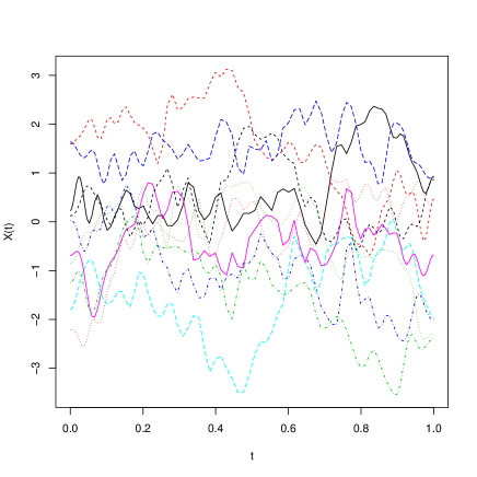
We first compare the performance of the estimated coefficient function through the FPCA approach proposed by Kato (2012) and our proposed approach under the RKHS framework. In particular, the functional covariate is generated as Xi(t)=k=150ζkξikψksubscript𝑋𝑖𝑡superscriptsubscript𝑘150subscript𝜁𝑘subscript𝜉𝑖𝑘subscript𝜓𝑘X_{i}(t)=\sum_{k=1}^{50}\zeta_{k}\xi_{ik}\psi_{k} for i=1,,n𝑖1𝑛i=1,\ldots,n, where ζk=4(1)k+1k2subscript𝜁𝑘4superscript1𝑘1superscript𝑘2\zeta_{k}=4\cdot(-1)^{k+1}\cdot k^{-2}, and ψ1=1subscript𝜓11\psi_{1}=1 and ψk=2cos((k1)πt)subscript𝜓𝑘2𝑘1𝜋𝑡\psi_{k}=\sqrt{2}\cos((k-1)\pi t) for k2𝑘2k\geq 2 are the eigenfunctions of X𝑋X. The random coefficients ξiksubscript𝜉𝑖𝑘\xi_{ik}’s are i.i.d generated from uniform distribution on [3,3]33[-\sqrt{3},\sqrt{3}]. Figure 1 displays the trajectories of 10 randomly selected functional covariates. The response is generated as yi=α+01Xi(t)β(t)𝑑t+σϵisubscript𝑦𝑖𝛼superscriptsubscript01subscript𝑋𝑖𝑡𝛽𝑡differential-d𝑡𝜎subscriptitalic-ϵ𝑖y_{i}=\alpha+\int_{0}^{1}X_{i}(t)\beta(t)dt+\sigma\epsilon_{i}, where the intercept α=0.1𝛼0.1\alpha=0.1 and the coefficient function β(t)=et𝛽𝑡superscript𝑒𝑡\beta(t)=e^{-t}. We consider two different designs, normal distribution of mean 0 and student t𝑡t distribution with 3 degrees of freedom, for the random noise ϵitalic-ϵ\epsilon to accommodate both light and heavy tails. Different values of σ𝜎\sigma’s are chosen to deliver two signal-to-noise ratios (SNR): 10 and 5. 200 independent Monte Carlo simulations are run for each design, where n=200𝑛200n=200 curves are generated.

Refer to caption
Figure 1: Trajectories of the functional covariate from 10 randomly selected subjects in one simulation run.
Refer to caption
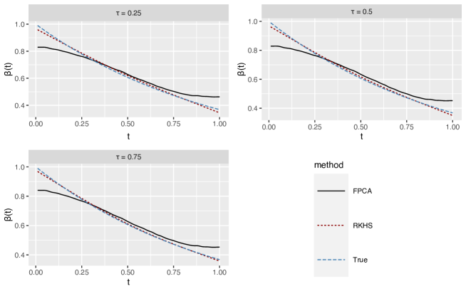
Figure 2: True slope function β(t)𝛽𝑡\beta(t) and estimates from FPAC and RKHS based methods. In each panel, the solid black line represents the estimate from the FPCA-based method, while the dashed blue line and the dotted red line represent the true coefficient function and the estimate from the proposed method, respectively.

To implement our proposed method, we take m=2𝑚2m=2 for the choice of Hm(𝕀)superscript𝐻𝑚𝕀H^{m}(\mathbb{I}) and adopt the Silverman (1986)’s rule-of-thumb (ROT) bandwidth to choose hh in kernel smoothing for saving computational cost. More specifically, we first fit a standard quantile regression of Y𝑌Y with respect to zij=Xi(t)gj(t)𝑑tsubscript𝑧𝑖𝑗subscript𝑋𝑖𝑡subscript𝑔𝑗𝑡differential-d𝑡z_{ij}=\int X_{i}(t)g_{j}(t)dt, where g1=1,g2(t)=t0.5formulae-sequencesubscript𝑔11subscript𝑔2𝑡𝑡0.5g_{1}=1,g_{2}(t)=t-0.5 and gj(t)=ξj2(t)subscript𝑔𝑗𝑡subscript𝜉𝑗2𝑡g_{j}(t)=\xi_{j-2}(t) for j=3,,2+n𝑗32𝑛j=3,\ldots,2+n. Then the ROT bandwidth is given by hROT=1.06s^n1/5subscriptROT1.06^𝑠superscript𝑛15h_{\text{ROT}}=1.06\hat{s}n^{-1/5}, where s^^𝑠\hat{s} is the minimum of the estimated standard error and the interquartile range (divided by 1.39) of the residuals from fitting the standard quantile regression. To choose the other tuning parameter λ𝜆\lambda, we employ the five-fold cross validation, where the smoothed empirical loss function R^hsubscript^𝑅\hat{R}_{h} defined in Equation (2.5) is used to compare the performance of the estimators generated from different λ𝜆\lambda’s. The optimal λ𝜆\lambda that minimizes this empirical loss turns out to be around 1×1061superscript1061\times 10^{-6}.

We consider three different quantile levels (τ=0.25,0.5,0.75𝜏0.250.50.75\tau=0.25,0.5,0.75) to compare these two approaches. In particular, for each τ𝜏\tau, we define the mean squared integration error of the estimated slope function β^(,τ)^𝛽𝜏\hat{\beta}(\cdot,\tau) as MISE(β^(,τ))=01{β^(t,τ)β(t)}2𝑑tMISE^𝛽𝜏superscriptsubscript01superscript^𝛽𝑡𝜏𝛽𝑡2differential-d𝑡\text{MISE}(\hat{\beta}(\cdot,\tau))=\int_{0}^{1}\{\hat{\beta}(t,\tau)-\beta(t)\}^{2}dt. Table 1 summarizes MISEs of the estimated coefficient functions using these two methods. Our proposed estimator compares favorably with the one using the FPCA method regardless of the distribution of the random error and the quantile level. This is also demonstrated by Figure 2. Figure 2 displays the average of the estimated coefficient functions across the 200 simulation runs for normally distributed errors under SNR = 10. For these three quantile levels (τ=0.25,0.5,0.75𝜏0.250.50.75\tau=0.25,0.5,0.75), the mean estimate generated from our proposed approach is nearly unbiased, while the counterpart from the FPCA method does not behave well near the boundaries.

Distribution SNR τ=0.25𝜏0.25\tau=0.25 τ=0.5𝜏0.5\tau=0.5 τ=0.75𝜏0.75\tau=0.75
FPCA RKHS FPCA RKHS FPCA RKHS
Normal 10 1.60 (1.58) 0.55 (0.57) 1.47 (1.42) 0.29 (0.30) 1.53 (1.60) 0.33 (0.32)
Normal 5 2.73 (1.73) 0.95 (0.98) 2.57 (1.44) 0.53 (0.56) 2.85 (2.08) 0.64 (0.73)
t3subscript𝑡3t_{3} 10 0.88 (1.05) 0.37 (0.34) 0.61 (0.72) 0.19 (0.20) 0.81 (0.93) 0.15 (0.16)
t3subscript𝑡3t_{3} 5 1.72 (1.53) 0.58 (0.56) 1.39 (1.40) 0.31 (0.35) 1.82 (1.52) 0.28 (0.32)
Table 1: Summary of averages and standard errors of MISE (×102)\times 10^{-2}) for the estimated slope functions based on the FPCA method and the RKHS method in different scenarios across 200 simulation runs.
τ𝜏\tau SNR = 10 SNR = 5
0.1 0.5 0.9 0.1 0.5 0.9
0.25 0.947 0.967 0.950 0.950 0.975 0.950
0.5 0.957 0.947 0.930 0.960 0.940 0.940
0.75 0.940 0.923 0.943 0.925 0.925 0.945
Table 2: Coverage probabilities of β0(t,τ)subscript𝛽0𝑡𝜏\beta_{0}(t,\tau) at t=0.1,0.5𝑡0.10.5t=0.1,0.5 and 0.9 and τ{0.25,0.5,0.75}𝜏0.250.50.75\tau\in\{0.25,0.5,0.75\}.

4.2 Confidence intervals/bands for β(,τ)𝛽𝜏\beta(\cdot,\tau)

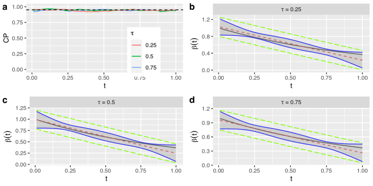
In this section we study the performance of the pointwise confidence intervals introduced in Remark 3.3 and the SCB in Remark 3.4. Panel (a) in Figure 3 displays the coverage probabilities of the pointwise confidence intervals for normally distributed errors with SNR = 10. For all of these three quantile levels, the true coverage probabilities are always close to the nominal level 95%. Panels (b) - (d) depict the estimated coefficient function based on our proposed method and the corresponding pointwise confidence intervals and the SCB from one random instance for the three quantile levels. The estimated coefficient function provides a reasonable estimate of the true coefficient function for all three quantile levels and the SCB fully covers the true slope function. Table 2 details the coverage probability of β^(t,τ)^𝛽𝑡𝜏\hat{\beta}(t,\tau) for β0(t,τ)subscript𝛽0𝑡𝜏\beta_{0}(t,\tau) at t={0.1,0.5,0.9}𝑡0.10.50.9t=\{0.1,0.5,0.9\} and τ={0.25,0.5,0.75}𝜏0.250.50.75\tau=\{0.25,0.5,0.75\}. Even with a moderate number of training curves (n=200𝑛200n=200), the true coverage probabilities are close to the nominal level 95% for both of these two signal to noise levels.

Refer to caption
Figure 3: (a): The true coverage probability of the pointwise confidence intervals across 200 simulations for normally distributed errors with SNR = 10. (b)-(d): In each panel, the solid black line represents the true slope function, while the dashed red line represents the estimated slope function from one random simulation run. The solid blue lines and the dashed green lines represent 95% pointwise confidence intervals and a 95% SCB, respectively.

4.3 Inference on the conditional quantile

We investigate the confidence intervals for conditional quantile proposed in Section 3.3. In addition to the training sample that consists of n=200𝑛200n=200 or 400 curves and scalar responses, we generate a new observation x0(t)subscript𝑥0𝑡x_{0}(t) and its corresponding response variable y0subscript𝑦0y_{0}; this new observation pair is fixed across B=200𝐵200B=200 simulation runs. To evaluate the converage probability of the constructed confidence interval for the conditional quantile given x0subscript𝑥0x_{0}, in each simulation run we implement the proposed estimation procedure on the independently generated training sample to generate a 95% confidence interval. The true coverage probability is approximated by the frequency of covering the true conditional quantile of y0subscript𝑦0y_{0} given x0subscript𝑥0x_{0} across 200 simulations. Table 3 summarizes the coverage probabilities of the constructed confidence interval in different designs. Regardless of sample size or SNR levels, the true coverage probability is always close to the nominal level 95%. When the SNR is fixed, increasing the size of the training sample can yield confidence intervals for the conditional quantile with a true coverage probability closer to the nominal level.

τ𝜏\tau n=200𝑛200n=200 n=400𝑛400n=400
SNR = 10 SNR = 5 SNR = 10 SNR = 5
0.25 0.940 0.940 0.950 0.950
0.5 0.945 0.945 0.950 0.955
0.75 0.930 0.920 0.940 0.940
Table 3: Coverage probabilities of conditional quantile.

5 Real example

In this section, we apply the proposed method to one real-world example to demonstrate its performance.

Alzheimer’s disease (AD) is the most common cause of dementia, a general term for the impaired cognitive abilities such as memorizing, thinking, or making decisions that interferes with daily life. According to Ferreira and Busatto (2011), clinicians usually leverage a history of progressive and characteristic cognitive decline and the presence of objective cognitive deficits in the diagnosis of AD. Examinations leveraging neuroimaging plays a critical role in the diagnostic investigation of dementia. In particular, these examinations can not only facilitate identification of non-AD pathological processes that are related to cognitive decline but also are useful to pinpoint informative biomarkers that can help to enhance the diagnosis of AD. Substantial studies have shown correlations between quantitative measures collected by magnetic resonance brain imaging and AD progression (Ledig et al., 2018).

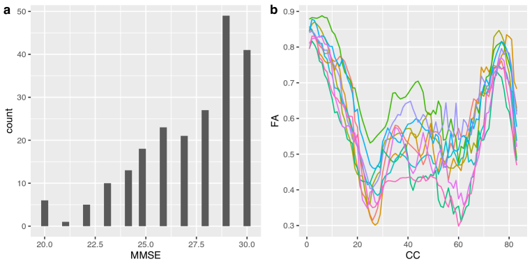
Refer to caption
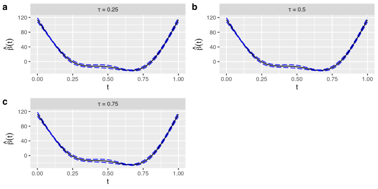
Figure 4: (a): Histogram of the MMSE scores from n=214𝑛214n=214 subject. (b): The trajectories of FA values measured at 83 different locations along CC from 10 randomly selected subjects.

In this study, we obtained the data from the ongoing Alzheimer’s Disease Neuroimaging Initiative (ADNI), that unites researchers working to define the progression of AD. Particularly, the ADNI aims to determine the relationships between clinical, cognitive, imaging, genetic, and biochemical biomarkers over the whole range of AD progression. In this dataset, the functional covariate X𝑋X is fractional anisotropy (FA) collected by diffusion tensor imaging. The FA values were measured at 83 locations along the corpus callosum (CC) fiber tract for each subject. Panel (b) in Figure 4 depicts the FA trajectories of 10 randomly selected subjects. The scalar response of interest, Y𝑌Y, is the mini-mental state examination (MMSE) scores. We chose MMSE as the response since it is one of the most widely used test of cognitive functions for assessing the level of dementia a patient may have. Various functional regression models have been proposed to model the relations between the MMSE and FA trajectories; see Zhu et al. (2012) and Tang et al. (2021) for instance. Panel (a) in Figure 4 displays the histogram of the MMSE. Obviously the distribution of Y𝑌Y is highly left skewed, hence a simple summary statistic like sample mean cannot adequately describe the (conditional) distribution of Y𝑌Y given X𝑋X. We are concerned about using functional linear quantile regression to provide a comprehensive characterization of the conditional distribution of the MMSE in this study.

After removing 3 subjects with missing values in FA trajectories, n=214𝑛214n=214 subjects were retained in our analysis. To compare the prediction performance of the FPCA-based method by Kato (2012) and our RKHS-based method, a training set with 80% of all subjects were randomly selected and the remaining subjects constituted the test set. To better assess prediction accuracy, we randomly splitted the whole dataset 500 times with this ratio. Table 4 summarizes the mean prediction error, which is the average loss function (ρτ()subscript𝜌𝜏\rho_{\tau}(\cdot)) calculated on the test set, and the standard errors across the 500 splits for these two methods. Our proposed method outperforms its counterpart in terms of prediction accuracy in all of these three quantile levels.

Method τ=0.25𝜏0.25\tau=0.25 τ=0.5𝜏0.5\tau=0.5 τ=0.75𝜏0.75\tau=0.75
FPCA 2.63 (1.46) 2.41 (0.95) 0.80 (0.25)
RKHS 0.90 (0.11) 1.01 (0.11) 0.69 (0.08)
Table 4: Summary of averages and standard errors of prediction errors based on the FPCA method and the RKHS method across the 500 random splits.

Figure 5 depicts the estimated slope functions from minimizing Equation (2.7) for the above three quantile levels. In addition, the corresponding 95% pointwise confidence intervals for each estimated slope function are also displayed in Figure 5. Note t𝑡t denotes the rescaled CC in Figure 4. We follow the idea of Yao et al. (2005) to employ the one-curve-leave-out analysis to obtain pointwise confidence intervals, which are depicted in Figure 5. These intervals suggest that the FA trajectory has a time-vary effect on the conditional quantile of the MMSE scores, and this effect becomes weaker at the middle range of the CC fiber tract.

Refer to caption
Figure 5: Estimated coefficient functions and the corresponding 95% pointwise confidence intervals for τ{0.25,0.5,0.75}𝜏0.250.50.75\tau\in\{0.25,0.5,0.75\}.

6 Conclusions

In this paper we employ the kernel convolution technique to smooth the ordinary loss function in FLQR. Under the framework of RKHS, we establish a functional Bahadur representation for the minimizer of the regularized and smoothed empirical risk function. Then we develop inference tools such as pointwise confidence intervals and a SCB for the coefficient function. With the aid of the representer theorem, we design a gradient descent algorithm to facilitate estimation of the intercept and the coefficient function in FLQR. This algorithm is essentially different from that based on FPCA proposed by Kato (2012). Furthermore, empirical studies demonstrate that our proposed estimator outperforms the latter in finite sample.

Traditional theoretical work on FLQR was focused on estimation consistency and/or convergence rates. For instance, Kato (2012) studied the minimax rate in the estimation of the coefficient function and the conditional quantile function. Yao et al. (2017) established the convergence rate of the estimated coefficient function in a partially FLQR model where a functional covariate as well as a finite-dimensional covariate is considered. In contrast, little work has been done to develop statistical inferences for this model. Though Li et al. (2016) is an exception, this work imposes strong assumptions on the coefficient function. In contrast, mild conditions are required for it under the theoretical framework developed in this paper.

Appendix A Proof of Lemmas and Theorems

The section contains the proofs of the lemma and theorems in the main manuscript.

A.1 Proof of Lemma 3.1

Under Assumption A1, we obtain a Taylor expansion

f(u+hz|x)=j=0sf(j)(u|x)(hz)jj!+(hz)s(s1)!01(1w)s1[f(s)(u+whz|x)f(s)(u|x)]𝑑w.𝑓𝑢conditional𝑧𝑥superscriptsubscript𝑗0𝑠superscript𝑓𝑗conditional𝑢𝑥superscript𝑧𝑗𝑗superscript𝑧𝑠𝑠1superscriptsubscript01superscript1𝑤𝑠1delimited-[]superscript𝑓𝑠𝑢conditional𝑤𝑧𝑥superscript𝑓𝑠conditional𝑢𝑥differential-d𝑤f(u+hz|x)=\sum_{j=0}^{s}f^{(j)}(u|x)\frac{(hz)^{j}}{j!}+\frac{(hz)^{s}}{(s-1)!}\int_{0}^{1}(1-w)^{s-1}\left[f^{(s)}(u+whz|x)-f^{(s)}(u|x)\right]dw.

Recall that for any xsupp(X)𝑥supp𝑋x\in\mbox{supp}(X),

E[kh(uY)|x]f(u|x)Edelimited-[]conditionalsubscript𝑘𝑢𝑌𝑥𝑓conditional𝑢𝑥\displaystyle{\rm E}\,[k_{h}(u-Y)|x]-f(u|x) =kh(uy)f(y|x)𝑑yf(u|x)=k(z)[f(u+hz|x)f(u|x)]𝑑zabsentsubscript𝑘𝑢𝑦𝑓conditional𝑦𝑥differential-d𝑦𝑓conditional𝑢𝑥𝑘𝑧delimited-[]𝑓𝑢conditional𝑧𝑥𝑓conditional𝑢𝑥differential-d𝑧\displaystyle=\int k_{h}(u-y)f(y|x)dy-f(u|x)=\int k(z)\left[f(u+hz|x)-f(u|x)\right]dz
=01(1w)s1(hz)s(s1)!k(z)[f(s)(u+whz|x)f(s)(u|x)]𝑑z𝑑wabsentsuperscriptsubscript01superscript1𝑤𝑠1superscript𝑧𝑠𝑠1𝑘𝑧delimited-[]superscript𝑓𝑠𝑢conditional𝑤𝑧𝑥superscript𝑓𝑠conditional𝑢𝑥differential-d𝑧differential-d𝑤\displaystyle=\int_{0}^{1}(1-w)^{s-1}\int\frac{(hz)^{s}}{(s-1)!}k(z)\left[f^{(s)}(u+whz|x)-f^{(s)}(u|x)\right]dzdw (A1)

(i) As the check function can be written as

ρτ(u)𝑑G(u)=(1τ)0G(v)𝑑v+τ0[1G(u)]𝑑usubscript𝜌𝜏𝑢differential-d𝐺𝑢1𝜏superscriptsubscript0𝐺𝑣differential-d𝑣𝜏superscriptsubscript0delimited-[]1𝐺𝑢differential-d𝑢\int\rho_{\tau}(u)dG(u)=(1-\tau)\int_{-\infty}^{0}G(v)dv+\tau\int_{0}^{\infty}[1-G(u)]du

for any cdf G𝐺G. Therefore,

R(θ;τ)={(1τ)0v+Rx,θf(u|x)𝑑u𝑑v+τ0v+Rx,θf(u|x)𝑑u𝑑v}𝑑PX(x).𝑅𝜃𝜏1𝜏superscriptsubscript0superscriptsubscript𝑣subscript𝑅𝑥𝜃𝑓conditional𝑢𝑥differential-d𝑢differential-d𝑣𝜏subscriptsuperscript0subscriptsuperscript𝑣subscript𝑅𝑥𝜃𝑓conditional𝑢𝑥differential-d𝑢differential-d𝑣differential-dsubscript𝑃𝑋𝑥R(\theta;\tau)=\int\left\{(1-\tau)\int_{-\infty}^{0}\int_{-\infty}^{v+\langle R_{\scriptscriptstyle x},\theta\rangle}f(u|x)dudv+\tau\int^{\infty}_{0}\int^{\infty}_{v+\langle R_{\scriptscriptstyle x},\theta\rangle}f(u|x)dudv\right\}dP_{X}(x).

Similarly, we have

Rh(θ;τ)subscript𝑅𝜃𝜏\displaystyle R_{h}(\theta;\tau) ={(1τ)0v+Rx,θE[kh(uY)|x]dudv\displaystyle=\int\left\{(1-\tau)\int_{-\infty}^{0}\int_{-\infty}^{v+\langle R_{\scriptscriptstyle x},\theta\rangle}{\rm E}\,[k_{h}(u-Y)|x]dudv\right.
+τ0v+Rx,θE[kh(uY)|x]dudv}dPX(x).\displaystyle\quad\quad+\left.\tau\int^{\infty}_{0}\int^{\infty}_{v+\langle R_{\scriptscriptstyle x},\theta\rangle}{\rm E}\,[k_{h}(u-Y)|x]dudv\right\}dP_{X}(x).

Under Assumption A2, integrating (A1) yields

L1subscript𝐿1\displaystyle L_{1} :=|0v+Rx,θ{E[kh(uY)|x]f(u|x)}dudv|\displaystyle:=\left|\int_{-\infty}^{0}\int_{-\infty}^{v+\langle R_{\scriptscriptstyle x},\theta\rangle}\left\{{\rm E}\,[k_{h}(u-Y)|x]-f(u|x)\right\}dudv\right|
=|01(1w)s1(hz)s(s1)!k(z)0v+Rx,θ[f(s)(u+whz|x)f(s)(u|x)]dudvdzdw|\displaystyle=\left|\int_{0}^{1}(1-w)^{s-1}\int\frac{(hz)^{s}}{(s-1)!}k(z)\int_{-\infty}^{0}\int_{-\infty}^{v+\langle R_{\scriptscriptstyle x},\theta\rangle}\left[f^{(s)}(u+whz|x)-f^{(s)}(u|x)\right]dudvdzdw\right|
=|01(1w)s1(hz)s(s1)!k(z)[f(s2)(Rx,θ+whz|x)f(s2)(Rx,θ|x)]dzdw|\displaystyle=\left|\int_{0}^{1}(1-w)^{s-1}\int\frac{(hz)^{s}}{(s-1)!}k(z)\left[f^{(s-2)}(\langle R_{\scriptscriptstyle x},\theta\rangle+whz|x)-f^{(s-2)}(\langle R_{\scriptscriptstyle x},\theta\rangle|x)\right]dzdw\right|
Chs+1absent𝐶superscript𝑠1\displaystyle\leq Ch^{s+1}

since |zs+1k(z)|𝑑z<superscript𝑧𝑠1𝑘𝑧differential-d𝑧\int|z^{s+1}k(z)|dz<\infty by Assumption A2 and that f(s2)(|x)f^{(s-2)}(\cdot|x) is Lipschitz by Assumption A1. Using the same technique, we are able to show that

|0v+Rx,θ{E[kh(uY)|x]f(u|x)}dudv|Chs+1\left|\int^{\infty}_{0}\int^{\infty}_{v+\langle R_{\scriptscriptstyle x},\theta\rangle}\left\{{\rm E}\,[k_{h}(u-Y)|x]-f(u|x)\right\}dudv\right|\leq Ch^{s+1}

for some constant C𝐶C. This establishes (i).

(ii) By the Lebesgue dominated convergence theorem, we have

R(1)(θ;τ)θ1=E[(F(RX,θ|X)τ)RX,θ1]=[Rx,θf(y|x)𝑑yτ]Rx,θ1𝑑PX(x),superscript𝑅1𝜃𝜏subscript𝜃1Edelimited-[]𝐹conditionalsubscript𝑅𝑋𝜃𝑋𝜏subscript𝑅𝑋subscript𝜃1delimited-[]superscriptsubscriptsubscript𝑅𝑥𝜃𝑓conditional𝑦𝑥differential-d𝑦𝜏subscript𝑅𝑥subscript𝜃1differential-dsubscript𝑃𝑋𝑥R^{(1)}(\theta;\tau)\theta_{1}={\rm E}\,\left[\big{(}F(\langle R_{\scriptscriptstyle X},\theta\rangle|X)-\tau\big{)}\langle R_{\scriptscriptstyle X},\theta_{1}\rangle\right]=\int\left[\int_{-\infty}^{\langle R_{\scriptscriptstyle x},\theta\rangle}f(y|x)dy-\tau\right]\langle R_{\scriptscriptstyle x},\theta_{1}\rangle dP_{X}(x),

and

Rh(1)(θ;τ)θ1subscriptsuperscript𝑅1𝜃𝜏subscript𝜃1\displaystyle R^{(1)}_{h}(\theta;\tau)\theta_{1} =E{[K¯(RX,θYh)τ]RX,θ1}absentEdelimited-[]¯𝐾subscript𝑅𝑋𝜃𝑌𝜏subscript𝑅𝑋subscript𝜃1\displaystyle={\rm E}\,\left\{\left[\mkern 1.5mu\overline{\mkern-1.5muK\mkern-1.5mu}\mkern 1.5mu\left(\frac{\langle R_{\scriptscriptstyle X},\theta\rangle-Y}{h}\right)-\tau\right]\langle R_{\scriptscriptstyle X},\theta_{1}\rangle\right\}
={Rx,θE[kh(uY|x)]𝑑uτ}Rx,θ1𝑑PX(x).absentsuperscriptsubscriptsubscript𝑅𝑥𝜃Edelimited-[]subscript𝑘𝑢conditional𝑌𝑥differential-d𝑢𝜏subscript𝑅𝑥subscript𝜃1differential-dsubscript𝑃𝑋𝑥\displaystyle=\int\left\{\int_{-\infty}^{\langle R_{\scriptscriptstyle x},\theta\rangle}{\rm E}\,[k_{h}(u-Y|x)]du-\tau\right\}\langle R_{\scriptscriptstyle x},\theta_{1}\rangle dP_{X}(x).

As usk(u)𝑑u=0superscript𝑢𝑠𝑘𝑢differential-d𝑢0\int u^{s}k(u)du=0 and |us+1k(u)|𝑑u<superscript𝑢𝑠1𝑘𝑢differential-d𝑢\int|u^{s+1}k(u)|du<\infty, by integrating (A1) we have

L2subscript𝐿2\displaystyle L_{2} :=|Rx,θE[kh(uY|x)]f(u|x)du|\displaystyle:=\bigg{|}\int_{-\infty}^{\langle R_{\scriptscriptstyle x},\theta\rangle}{\rm E}\,[k_{h}(u-Y|x)]-f(u|x)du\bigg{|}
=|01(1w)s1(hz)s(s1)!k(z)Rx,θ[f(s)(u+whz|x)f(s)(u|x)]dudzdw|\displaystyle=\left|\int_{0}^{1}(1-w)^{s-1}\int\frac{(hz)^{s}}{(s-1)!}k(z)\int_{-\infty}^{\langle R_{\scriptscriptstyle x},\theta\rangle}\left[f^{(s)}(u+whz|x)-f^{(s)}(u|x)\right]dudzdw\right|
=|01(1w)s1(hz)s(s1)!k(z)[f(s1)(Rx,θ+whz|x)f(s1)(Rx,θ|x)]dzdw|\displaystyle=\left|\int_{0}^{1}(1-w)^{s-1}\int\frac{(hz)^{s}}{(s-1)!}k(z)\left[f^{(s-1)}(\langle R_{\scriptscriptstyle x},\theta\rangle+whz|x)-f^{(s-1)}(\langle R_{\scriptscriptstyle x},\theta\rangle|x)\right]dzdw\right|
=|01(1w)s1(hz)s+1(s1)!k(z)01f(s)(Rx,θ+twhz|x)dtdzdw|\displaystyle=\left|\int_{0}^{1}(1-w)^{s-1}\int\frac{(hz)^{s+1}}{(s-1)!}k(z)\int_{0}^{1}f^{(s)}(\langle R_{\scriptscriptstyle x},\theta\rangle+twhz|x)dtdzdw\right|
Chs+1,absent𝐶superscript𝑠1\displaystyle\leq Ch^{s+1},

uniformly given the fact that f(s)superscript𝑓𝑠f^{(s)} is bounded.

It follows that

Rh(1)(θ;τ)θ1R(1)(θ;τ)θ1subscriptsuperscript𝑅1𝜃𝜏subscript𝜃1superscript𝑅1𝜃𝜏subscript𝜃1\displaystyle R^{(1)}_{h}(\theta;\tau)\theta_{1}-R^{(1)}(\theta;\tau)\theta_{1} Chs+1E[|RX,θ1|]absent𝐶superscript𝑠1Edelimited-[]subscript𝑅𝑋subscript𝜃1\displaystyle\leq Ch^{s+1}{\rm E}\,[|\langle R_{\scriptscriptstyle X},\theta_{1}\rangle|]
Chs+1[E(RX,θ14)]1/4Chs+1θ1absent𝐶superscript𝑠1superscriptdelimited-[]Esuperscriptsubscript𝑅𝑋subscript𝜃1414𝐶superscript𝑠1normsubscript𝜃1\displaystyle\leq Ch^{s+1}\left[{\rm E}\,\left(\langle R_{X},\theta_{1}\rangle^{4}\right)\right]^{1/4}\leq Ch^{s+1}\|\theta_{1}\|

by the Cauchy-Schwarz inequality and Lemma S.3 of Shang and Cheng (2015b). This establish (ii).

(iii) The second order Fréchet derivative operator of R(θ;τ)𝑅𝜃𝜏R(\theta;\tau) satisfies

R(2)(θ;τ)θ1θ2=E[f(RX,θ|X)RX,θ1RX,θ2]=f(Rx,θ|x)Rx,θ1Rx,θ2𝑑PX(x),superscript𝑅2𝜃𝜏subscript𝜃1subscript𝜃2Edelimited-[]𝑓conditionalsubscript𝑅𝑋𝜃𝑋subscript𝑅𝑋subscript𝜃1subscript𝑅𝑋subscript𝜃2𝑓conditionalsubscript𝑅𝑥𝜃𝑥subscript𝑅𝑥subscript𝜃1subscript𝑅𝑥subscript𝜃2differential-dsubscript𝑃𝑋𝑥R^{(2)}(\theta;\tau)\theta_{1}\theta_{2}={\rm E}\,\left[f(\langle R_{\scriptscriptstyle X},\theta\rangle|X)\langle R_{\scriptscriptstyle X},\theta_{1}\rangle\langle R_{\scriptscriptstyle X},\theta_{2}\rangle\right]=\int f(\langle R_{\scriptscriptstyle x},\theta\rangle|x)\langle R_{\scriptscriptstyle x},\theta_{1}\rangle\langle R_{\scriptscriptstyle x},\theta_{2}\rangle dP_{X}(x),

and, analogously,

Rh(2)(θ;τ)θ1θ2subscriptsuperscript𝑅2𝜃𝜏subscript𝜃1subscript𝜃2\displaystyle R^{(2)}_{h}(\theta;\tau)\theta_{1}\theta_{2} =E[kh(RX,θY)RX,θ1RX,θ2]absentEdelimited-[]subscript𝑘subscript𝑅𝑋𝜃𝑌subscript𝑅𝑋subscript𝜃1subscript𝑅𝑋subscript𝜃2\displaystyle={\rm E}\,\left[k_{h}(\langle R_{\scriptscriptstyle X},\theta\rangle-Y)\langle R_{\scriptscriptstyle X},\theta_{1}\rangle\langle R_{\scriptscriptstyle X},\theta_{2}\rangle\right]
=E[kh(Rx,θY|x)]Rx,θ1Rx,θ2𝑑PX(x).absentEdelimited-[]subscript𝑘subscript𝑅𝑥𝜃conditional𝑌𝑥subscript𝑅𝑥subscript𝜃1subscript𝑅𝑥subscript𝜃2differential-dsubscript𝑃𝑋𝑥\displaystyle=\int{\rm E}\,\left[k_{h}(\langle R_{\scriptscriptstyle x},\theta\rangle-Y|x)\right]\langle R_{\scriptscriptstyle x},\theta_{1}\rangle\langle R_{\scriptscriptstyle x},\theta_{2}\rangle dP_{X}(x).

Setting u=Rx,θ𝑢subscript𝑅𝑥𝜃u=\langle R_{\scriptscriptstyle x},\theta\rangle. In light of (A1), we have

|E[kh(uY)|x]f(u|x)|\displaystyle\left|{\rm E}\,\left[k_{h}(u-Y)|x\right]-f(u|x)\right|
Chs|zsk(z)|sup(y,x)×supp(X)supt:|t|hz|f(s)(y+t|x)f(s)(y|x)|dz\displaystyle\leq Ch^{s}\int|z^{s}k(z)|\sup_{(y,x)\in\mathbb{R}\times\mbox{supp}(X)}\sup_{t:|t|\leq hz}\left|f^{(s)}(y+t|x)-f^{(s)}(y|x)\right|dz
=o(hs)absent𝑜superscript𝑠\displaystyle=o(h^{s})

under Assumption A1 and Assumption A2.

Then following the proof of part (ii), it is easy to verify that
|Rh(1)(θ;τ)θ1θ2R(1)(θ;τ)θ1θ2|=o(hs)θ1θ2subscriptsuperscript𝑅1𝜃𝜏subscript𝜃1subscript𝜃2superscript𝑅1𝜃𝜏subscript𝜃1subscript𝜃2𝑜superscript𝑠normsubscript𝜃1normsubscript𝜃2|R^{(1)}_{h}(\theta;\tau)\theta_{1}\theta_{2}-R^{(1)}(\theta;\tau)\theta_{1}\theta_{2}|=o(h^{s})\|\theta_{1}\|\|\theta_{2}\|. This establishes (iii).

(iv) Note that

Rh(2)(θ;τ)θ1θ2subscriptsuperscript𝑅2𝜃𝜏subscript𝜃1subscript𝜃2\displaystyle R^{(2)}_{h}(\theta;\tau)\theta_{1}\theta_{2} =E[kh(RX,θY)RX,θ1RX,θ2]absentEdelimited-[]subscript𝑘subscript𝑅𝑋𝜃𝑌subscript𝑅𝑋subscript𝜃1subscript𝑅𝑋subscript𝜃2\displaystyle={\rm E}\,\left[k_{h}(\langle R_{\scriptscriptstyle X},\theta\rangle-Y)\langle R_{\scriptscriptstyle X},\theta_{1}\rangle\langle R_{\scriptscriptstyle X},\theta_{2}\rangle\right]
=k(z)f(Rx,θ+hz|x)Rx,θ1Rx,θ2𝑑PX(x)𝑑z.absent𝑘𝑧𝑓subscript𝑅𝑥𝜃conditional𝑧𝑥subscript𝑅𝑥subscript𝜃1subscript𝑅𝑥subscript𝜃2differential-dsubscript𝑃𝑋𝑥differential-d𝑧\displaystyle=\int k(z)\int f(\langle R_{\scriptscriptstyle x},\theta\rangle+hz|x)\langle R_{\scriptscriptstyle x},\theta_{1}\rangle\langle R_{\scriptscriptstyle x},\theta_{2}\rangle dP_{X}(x)dz.

Since f(|x)f(\cdot|x) is Lipschitz under Assumption A1 (d),

|Rh(2)(θ+θ;τ)θ1θ2Rh(2)(θ;τ)θ1θ2|superscriptsubscript𝑅2𝜃superscript𝜃𝜏subscript𝜃1subscript𝜃2superscriptsubscript𝑅2𝜃𝜏subscript𝜃1subscript𝜃2\displaystyle\left|R_{h}^{(2)}(\theta+\theta^{*};\tau)\theta_{1}\theta_{2}-R_{h}^{(2)}(\theta;\tau)\theta_{1}\theta_{2}\right|
C|k(z)||RX,θ||RX,θ1||RX,θ2|𝑑PX(x)𝑑zabsent𝐶𝑘𝑧subscript𝑅𝑋superscript𝜃subscript𝑅𝑋subscript𝜃1subscript𝑅𝑋subscript𝜃2differential-dsubscript𝑃𝑋𝑥differential-d𝑧\displaystyle\leq C\int|k(z)|\int|\langle R_{\scriptscriptstyle X},\theta^{*}\rangle||\langle R_{\scriptscriptstyle X},\theta_{1}\rangle||\langle R_{\scriptscriptstyle X},\theta_{2}\rangle|dP_{X}(x)dz
CE[|RX,θ||RX,θ1||RX,θ2|]absent𝐶Edelimited-[]subscript𝑅𝑋superscript𝜃subscript𝑅𝑋subscript𝜃1subscript𝑅𝑋subscript𝜃2\displaystyle\leq C{\rm E}\,[|\langle R_{\scriptscriptstyle X},\theta^{*}\rangle||\langle R_{\scriptscriptstyle X},\theta_{1}\rangle||\langle R_{\scriptscriptstyle X},\theta_{2}\rangle|]
C[E(RX,θ4)]1/4[E(RX,θ14)]1/4[E(RX,θ24)]1/4absent𝐶superscriptdelimited-[]Esuperscriptsubscript𝑅𝑋superscript𝜃414superscriptdelimited-[]Esuperscriptsubscript𝑅𝑋subscript𝜃1414superscriptdelimited-[]Esuperscriptsubscript𝑅𝑋subscript𝜃2414\displaystyle\leq C\left[{\rm E}\,\left(\langle R_{X},\theta^{\scriptscriptstyle*}\rangle^{4}\right)\right]^{1/4}\left[{\rm E}\,\left(\langle R_{X},\theta_{1}\rangle^{4}\right)\right]^{1/4}\left[{\rm E}\,\left(\langle R_{X},\theta_{2}\rangle^{4}\right)\right]^{1/4}
Cθθ1θ2absent𝐶normsuperscript𝜃normsubscript𝜃1normsubscript𝜃2\displaystyle\leq C\|\theta^{\scriptscriptstyle*}\|\|\theta_{1}\|\|\theta_{2}\|

uniformly in (θ,h,θ,τ)𝜃superscript𝜃𝜏(\theta,h,\theta^{*},\tau).

A.2 Proof of Theorem 3.1

Recall that R(θ;τ)=ρτ(u)E[dF^(u;θ)]𝑅𝜃𝜏subscript𝜌𝜏𝑢Edelimited-[]𝑑^𝐹𝑢𝜃R(\theta;\tau)=\int\rho_{\tau}(u){\rm E}\,[d\hat{F}(u;\theta)], where the expectation is taken with respect to the joint distribution of (X,Y)𝑋𝑌(X,Y). Since F^(u;θ)=1ni=1n𝟙(ϵi(θ)u)^𝐹𝑢𝜃1𝑛superscriptsubscript𝑖1𝑛1subscriptitalic-ϵ𝑖𝜃𝑢\hat{F}(u;\theta)=\frac{1}{n}\sum_{i=1}^{n}\mathbbm{1}(\epsilon_{i}(\theta)\leq u), EF^(u;θ)=P(ϵ(θ)u)E^𝐹𝑢𝜃𝑃italic-ϵ𝜃𝑢{\rm E}\,\hat{F}(u;\theta)=P(\epsilon(\theta)\leq u), where e(θ)=YRX,θ𝑒𝜃𝑌subscript𝑅𝑋𝜃e(\theta)=Y-\langle R_{X},\theta\rangle. Hence dE[F^(u;θ)]dufϵ(u;θ)𝑑Edelimited-[]^𝐹𝑢𝜃𝑑𝑢subscript𝑓italic-ϵ𝑢𝜃\frac{d{\rm E}\,[\hat{F}(u;\theta)]}{du}\equiv f_{\epsilon}(u;\theta), where fϵ(,θ)subscript𝑓italic-ϵ𝜃f_{\epsilon}(\cdot,\theta) denotes the marginal density of ϵ(θ):=YRX,θassignitalic-ϵ𝜃𝑌subscript𝑅𝑋𝜃\epsilon(\theta):=Y-\langle R_{X},\theta\rangle. It follows that R(θ;τ)=ρτ(u)fϵ(u;θ)𝑅𝜃𝜏subscript𝜌𝜏𝑢subscript𝑓italic-ϵ𝑢𝜃R(\theta;\tau)=\int\rho_{\tau}(u)f_{\epsilon}(u;\theta). Similarly, R^h(θ;τ)=1ni=1nρτ(u)kh(uϵi(θ))𝑑usubscript^𝑅𝜃𝜏1𝑛superscriptsubscript𝑖1𝑛subscript𝜌𝜏𝑢subscript𝑘𝑢subscriptitalic-ϵ𝑖𝜃differential-d𝑢\hat{R}_{h}(\theta;\tau)=\frac{1}{n}\sum_{i=1}^{n}\int\rho_{\tau}(u)k_{h}(u-\epsilon_{i}(\theta))du and Rh(θ;τ)=E[R^h(θ;τ)]=ρτ(u)E[kh(uϵ(θ))]𝑑usubscript𝑅𝜃𝜏Edelimited-[]subscript^𝑅𝜃𝜏subscript𝜌𝜏𝑢Edelimited-[]subscript𝑘𝑢italic-ϵ𝜃differential-d𝑢R_{h}(\theta;\tau)={\rm E}\,[\hat{R}_{h}(\theta;\tau)]=\int\rho_{\tau}(u){\rm E}\,[k_{h}(u-\epsilon(\theta))]du. Let K~h(u;θ)=E[kh(uϵ(θ))]subscript~𝐾𝑢𝜃Edelimited-[]subscript𝑘𝑢italic-ϵ𝜃\tilde{K}_{h}(u;\theta)={\rm E}\,[k_{h}(u-\epsilon(\theta))], where the expectation is taken with respect to the distribution of ϵ(θ)italic-ϵ𝜃\epsilon(\theta). In other words, K~h(u;θ)=fϵ(v;θ)kh(uv)𝑑vsubscript~𝐾𝑢𝜃subscript𝑓italic-ϵ𝑣𝜃subscript𝑘𝑢𝑣differential-d𝑣\tilde{K}_{h}(u;\theta)=\int f_{\epsilon}(v;\theta)k_{h}(u-v)dv and Rh(θ;τ)=ρτ(u)K~h(u;θ)𝑑usubscript𝑅𝜃𝜏subscript𝜌𝜏𝑢subscript~𝐾𝑢𝜃differential-d𝑢R_{h}(\theta;\tau)=\int\rho_{\tau}(u)\tilde{K}_{h}(u;\theta)du. So hλ(θ)=ρτ(u)K~h(u;θ)𝑑u+λ2J(β,β)subscript𝜆𝜃subscript𝜌𝜏𝑢subscript~𝐾𝑢𝜃differential-d𝑢𝜆2𝐽𝛽𝛽\ell_{h\lambda}(\theta)=\int\rho_{\tau}(u)\tilde{K}_{h}(u;\theta)du+\frac{\lambda}{2}J(\beta,\beta) based on the definition of hλsubscript𝜆\ell_{h\lambda} in (3.1).

The first-order Fréchet derivative of hλsubscript𝜆\ell_{h\lambda} w.r.t θ𝜃\theta satisfies that for any Δθ=(Δα,Δβ)Δ𝜃Δ𝛼Δ𝛽\Delta\theta=(\Delta\alpha,\Delta\beta)\in{\cal{H}},

Shλ(θ)ΔθDθhλ(θ)Δθ=ρτ(u)DθK~h(u;θ)Δθ𝑑u+Pλθ,Δθ,subscript𝑆𝜆𝜃Δ𝜃subscript𝐷𝜃subscript𝜆𝜃Δ𝜃subscript𝜌𝜏𝑢subscript𝐷𝜃subscript~𝐾𝑢𝜃Δ𝜃differential-d𝑢subscript𝑃𝜆𝜃Δ𝜃S_{h\lambda}(\theta)\Delta\theta\equiv D_{\theta}\ell_{h\lambda}(\theta)\Delta\theta=\int\rho_{\tau}(u)D_{\theta}\tilde{K}_{h}(u;\theta)\Delta\theta du+\langle P_{\lambda}\theta,\Delta\theta\rangle,

where Pλ(θ)=(0,Wλβ)subscript𝑃𝜆𝜃0subscript𝑊𝜆𝛽P_{\lambda}(\theta)=(0,W_{\lambda}\beta)\in{\cal{H}} and satisfies that Pλ(θ),θ~=Wλβ,β~1subscript𝑃𝜆𝜃~𝜃subscriptsubscript𝑊𝜆𝛽~𝛽1\langle P_{\lambda}(\theta),\tilde{\theta}\rangle=\langle W_{\lambda}\beta,\tilde{\beta}\rangle_{1} for any θ~=(α~,β~)~𝜃~𝛼~𝛽\tilde{\theta}=(\tilde{\alpha},\tilde{\beta})\in{\cal{H}} from Proposition 2.5 of Shang and Cheng (2015a). The second-order Fréchet derivative of hλsubscript𝜆\ell_{h\lambda} is

Dθ2hλ(θ)Δθ1Δθ2=ρτ(u)Dθ2K~h(u;θ)Δθ1Δθ2𝑑u+PλΔθ1,Δθ2.subscriptsuperscript𝐷2𝜃subscript𝜆𝜃Δsubscript𝜃1Δsubscript𝜃2subscript𝜌𝜏𝑢superscriptsubscript𝐷𝜃2subscript~𝐾𝑢𝜃Δsubscript𝜃1Δsubscript𝜃2differential-d𝑢subscript𝑃𝜆Δsubscript𝜃1Δsubscript𝜃2D^{2}_{\theta}\ell_{h\lambda}(\theta)\Delta\theta_{1}\Delta\theta_{2}=\int\rho_{\tau}(u)D_{\theta}^{2}\tilde{K}_{h}(u;\theta)\Delta\theta_{1}\Delta\theta_{2}du+\langle P_{\lambda}\Delta\theta_{1},\Delta\theta_{2}\rangle.

For notational brevity, we shall drop τ𝜏\tau from θ0h(τ)subscript𝜃0𝜏\theta_{0h}(\tau) if the quantile level is clear from the context. Since θ0hsubscript𝜃0\theta_{0h} minimizes Rh(θ;τ)subscript𝑅𝜃𝜏R_{h}(\theta;\tau), Shλ(θ0h)=Pλθ0hsubscript𝑆𝜆subscript𝜃0subscript𝑃𝜆subscript𝜃0S_{h\lambda}(\theta_{0h})=P_{\lambda}\theta_{0h}.

Define T1(θ)=θShλ(θ0+θ)subscript𝑇1𝜃𝜃subscript𝑆𝜆subscript𝜃0𝜃T_{1}(\theta)=\theta-S_{h\lambda}(\theta_{0}+\theta) for θ𝜃\theta\in{\cal{H}}, and let S0λ(θ0)=Pλθ0subscript𝑆0𝜆subscript𝜃0subscript𝑃𝜆subscript𝜃0S_{0\lambda}(\theta_{0})=P_{\lambda}\theta_{0}. Write T1(θ)subscript𝑇1𝜃T_{1}(\theta) as T1(θ)+S0λ(θ0)S0λ(θ0)subscript𝑇1𝜃subscript𝑆0𝜆subscript𝜃0subscript𝑆0𝜆subscript𝜃0T_{1}(\theta)+S_{0\lambda}(\theta_{0})-S_{0\lambda}(\theta_{0}). So T1(θ)T1(θ)+S0λ(θ0)+S0λ(θ0)normsubscript𝑇1𝜃normsubscript𝑇1𝜃subscript𝑆0𝜆subscript𝜃0normsubscript𝑆0𝜆subscript𝜃0\|T_{1}(\theta)\|\leq\|T_{1}(\theta)+S_{0\lambda}(\theta_{0})\|+\|S_{0\lambda}(\theta_{0})\|. For the first term, we have

T1(θ)+S0λ(θ0)subscript𝑇1𝜃subscript𝑆0𝜆subscript𝜃0\displaystyle T_{1}(\theta)+S_{0\lambda}(\theta_{0}) =θShλ(θ0+θ)+S0λ(θ0)absent𝜃subscript𝑆𝜆subscript𝜃0𝜃subscript𝑆0𝜆subscript𝜃0\displaystyle=\theta-S_{h\lambda}(\theta_{0}+\theta)+S_{0\lambda}(\theta_{0})
=θρτ(u)DθK~h(u;θ+θ0)𝑑uPλ(θ+θ0)absent𝜃subscript𝜌𝜏𝑢subscript𝐷𝜃subscript~𝐾𝑢𝜃subscript𝜃0differential-d𝑢subscript𝑃𝜆𝜃subscript𝜃0\displaystyle=\theta-\int\rho_{\tau}(u)D_{\theta}\tilde{K}_{h}(u;\theta+\theta_{0})du-P_{\lambda}(\theta+\theta_{0})
+ρτ(u)Dθfϵ(u;θ0)𝑑u+Pλθ0subscript𝜌𝜏𝑢subscript𝐷𝜃subscript𝑓italic-ϵ𝑢subscript𝜃0differential-d𝑢subscript𝑃𝜆subscript𝜃0\displaystyle\leavevmode\nobreak\ \leavevmode\nobreak\ \leavevmode\nobreak\ \leavevmode\nobreak\ +\int\rho_{\tau}(u)D_{\theta}f_{\epsilon}(u;\theta_{0})du+P_{\lambda}\theta_{0}
=θρτ(u)[DθK~h(u;θ+θ0)DθK~h(u;θ0)]𝑑uabsent𝜃subscript𝜌𝜏𝑢delimited-[]subscript𝐷𝜃subscript~𝐾𝑢𝜃subscript𝜃0subscript𝐷𝜃subscript~𝐾𝑢subscript𝜃0differential-d𝑢\displaystyle=\theta-\int\rho_{\tau}(u)[D_{\theta}\tilde{K}_{h}(u;\theta+\theta_{0})-D_{\theta}\tilde{K}_{h}(u;\theta_{0})]du
ρτ(u)DθK~h(u;θ0)𝑑uPλθ+ρτ(u)Dθfϵ(u;θ0)𝑑usubscript𝜌𝜏𝑢subscript𝐷𝜃subscript~𝐾𝑢subscript𝜃0differential-d𝑢subscript𝑃𝜆𝜃subscript𝜌𝜏𝑢subscript𝐷𝜃subscript𝑓italic-ϵ𝑢subscript𝜃0differential-d𝑢\displaystyle\leavevmode\nobreak\ \leavevmode\nobreak\ \leavevmode\nobreak\ \leavevmode\nobreak\ -\int\rho_{\tau}(u)D_{\theta}\tilde{K}_{h}(u;\theta_{0})du-P_{\lambda}\theta+\int\rho_{\tau}(u)D_{\theta}f_{\epsilon}(u;\theta_{0})du
=θρτ(u)[01Dθ2K~h(u;sθ+θ0)θ𝑑s]𝑑uabsent𝜃subscript𝜌𝜏𝑢delimited-[]superscriptsubscript01superscriptsubscript𝐷𝜃2subscript~𝐾𝑢𝑠𝜃subscript𝜃0𝜃differential-d𝑠differential-d𝑢\displaystyle=\theta-\int\rho_{\tau}(u)\left[\int_{0}^{1}D_{\theta}^{2}\tilde{K}_{h}(u;s\theta+\theta_{0})\theta ds\right]du
ρτ(u)[DθK~h(u;θ0)Dθfϵ(u;θ0)]𝑑uPλθ.subscript𝜌𝜏𝑢delimited-[]subscript𝐷𝜃subscript~𝐾𝑢subscript𝜃0subscript𝐷𝜃subscript𝑓italic-ϵ𝑢subscript𝜃0differential-d𝑢subscript𝑃𝜆𝜃\displaystyle\leavevmode\nobreak\ \leavevmode\nobreak\ \leavevmode\nobreak\ \leavevmode\nobreak\ -\int\rho_{\tau}(u)[D_{\theta}\tilde{K}_{h}(u;\theta_{0})-D_{\theta}f_{\epsilon}(u;\theta_{0})]du-P_{\lambda}\theta.

By the proof of Proposition 3.5 of Shang and Cheng (2015a), we know that
[ρτ(u)Dθ2fϵ(u;θ0)𝑑u+Pλ]θ=θdelimited-[]subscript𝜌𝜏𝑢subscriptsuperscript𝐷2𝜃subscript𝑓italic-ϵ𝑢subscript𝜃0differential-d𝑢subscript𝑃𝜆𝜃𝜃\left[\int\rho_{\tau}(u)D^{2}_{\theta}f_{\epsilon}(u;\theta_{0})du+P_{\lambda}\right]\theta=\theta. So

T1(θ)+S0λ(θ0)subscript𝑇1𝜃subscript𝑆0𝜆subscript𝜃0\displaystyle T_{1}(\theta)+S_{0\lambda}(\theta_{0}) =ρτ(u)Dθ2fϵ(u;θ0)θ𝑑u+Pλθρτ(u)[01Dθ2K~h(u;sθ+θ0)θ𝑑s]𝑑uabsentsubscript𝜌𝜏𝑢subscriptsuperscript𝐷2𝜃subscript𝑓italic-ϵ𝑢subscript𝜃0𝜃differential-d𝑢subscript𝑃𝜆𝜃subscript𝜌𝜏𝑢delimited-[]superscriptsubscript01superscriptsubscript𝐷𝜃2subscript~𝐾𝑢𝑠𝜃subscript𝜃0𝜃differential-d𝑠differential-d𝑢\displaystyle=\int\rho_{\tau}(u)D^{2}_{\theta}f_{\epsilon}(u;\theta_{0})\theta du+P_{\lambda}\theta-\int\rho_{\tau}(u)\left[\int_{0}^{1}D_{\theta}^{2}\tilde{K}_{h}(u;s\theta+\theta_{0})\theta ds\right]du
ρτ(u)[DθK~h(u;θ0)Dθfϵ(u;θ0)]𝑑uPλθsubscript𝜌𝜏𝑢delimited-[]subscript𝐷𝜃subscript~𝐾𝑢subscript𝜃0subscript𝐷𝜃subscript𝑓italic-ϵ𝑢subscript𝜃0differential-d𝑢subscript𝑃𝜆𝜃\displaystyle\leavevmode\nobreak\ \leavevmode\nobreak\ \leavevmode\nobreak\ \leavevmode\nobreak\ -\int\rho_{\tau}(u)[D_{\theta}\tilde{K}_{h}(u;\theta_{0})-D_{\theta}f_{\epsilon}(u;\theta_{0})]du-P_{\lambda}\theta
=ρτ(u)(01[Dθ2fϵ(u;θ0)θDθ2K~h(u;sθ+θ0)θ]𝑑s)𝑑uabsentsubscript𝜌𝜏𝑢superscriptsubscript01delimited-[]subscriptsuperscript𝐷2𝜃subscript𝑓italic-ϵ𝑢subscript𝜃0𝜃superscriptsubscript𝐷𝜃2subscript~𝐾𝑢𝑠𝜃subscript𝜃0𝜃differential-d𝑠differential-d𝑢\displaystyle=\int\rho_{\tau}(u)\left(\int_{0}^{1}[D^{2}_{\theta}f_{\epsilon}(u;\theta_{0})\theta-D_{\theta}^{2}\tilde{K}_{h}(u;s\theta+\theta_{0})\theta]ds\right)du
ρτ(u)[DθK~h(u;θ0)Dθfϵ(u;θ0)]du=:I+II.\displaystyle\leavevmode\nobreak\ \leavevmode\nobreak\ \leavevmode\nobreak\ \leavevmode\nobreak\ -\int\rho_{\tau}(u)[D_{\theta}\tilde{K}_{h}(u;\theta_{0})-D_{\theta}f_{\epsilon}(u;\theta_{0})]du=:\textup{I}+\textup{II}.

For I, we have

ρτ(u)[Dθ2K~h(u;sθ+θ0)Dθ2fϵ(u;θ0)]𝑑uopsubscriptdelimited-∥∥subscript𝜌𝜏𝑢delimited-[]superscriptsubscript𝐷𝜃2subscript~𝐾𝑢𝑠𝜃subscript𝜃0subscriptsuperscript𝐷2𝜃subscript𝑓italic-ϵ𝑢subscript𝜃0differential-d𝑢op\displaystyle\left\lVert\int\rho_{\tau}(u)[D_{\theta}^{2}\tilde{K}_{h}(u;s\theta+\theta_{0})-D^{2}_{\theta}f_{\epsilon}(u;\theta_{0})]du\right\rVert_{\mbox{op}}
=ρτ(u)[Dθ2K~h(u;sθ+θ0)Dθ2fϵ(u;sθ+θ0)+Dθ2fϵ(u;sθ+θ0)Dθ2fϵ(u;θ0)]opabsentsubscriptdelimited-∥∥subscript𝜌𝜏𝑢delimited-[]superscriptsubscript𝐷𝜃2subscript~𝐾𝑢𝑠𝜃subscript𝜃0subscriptsuperscript𝐷2𝜃subscript𝑓italic-ϵ𝑢𝑠𝜃subscript𝜃0subscriptsuperscript𝐷2𝜃subscript𝑓italic-ϵ𝑢𝑠𝜃subscript𝜃0subscriptsuperscript𝐷2𝜃subscript𝑓italic-ϵ𝑢subscript𝜃0op\displaystyle\leavevmode\nobreak\ \leavevmode\nobreak\ =\left\lVert\int\rho_{\tau}(u)[D_{\theta}^{2}\tilde{K}_{h}(u;s\theta+\theta_{0})-D^{2}_{\theta}f_{\epsilon}(u;s\theta+\theta_{0})+D^{2}_{\theta}f_{\epsilon}(u;s\theta+\theta_{0})-D^{2}_{\theta}f_{\epsilon}(u;\theta_{0})]\right\rVert_{\mbox{op}}
ρτ(u)[Dθ2K~h(u;sθ+θ0)Dθ2fϵ(u;sθ+θ0)]𝑑uopabsentsubscriptdelimited-∥∥subscript𝜌𝜏𝑢delimited-[]superscriptsubscript𝐷𝜃2subscript~𝐾𝑢𝑠𝜃subscript𝜃0subscriptsuperscript𝐷2𝜃subscript𝑓italic-ϵ𝑢𝑠𝜃subscript𝜃0differential-d𝑢op\displaystyle\leavevmode\nobreak\ \leavevmode\nobreak\ \leq\left\lVert\int\rho_{\tau}(u)[D_{\theta}^{2}\tilde{K}_{h}(u;s\theta+\theta_{0})-D^{2}_{\theta}f_{\epsilon}(u;s\theta+\theta_{0})]du\right\rVert_{\mbox{op}}
+ρτ(u)[Dθ2fϵ(u;sθ+θ0)Dθ2fϵ(u;θ0)]𝑑uopsubscriptdelimited-∥∥subscript𝜌𝜏𝑢delimited-[]subscriptsuperscript𝐷2𝜃subscript𝑓italic-ϵ𝑢𝑠𝜃subscript𝜃0subscriptsuperscript𝐷2𝜃subscript𝑓italic-ϵ𝑢subscript𝜃0differential-d𝑢op\displaystyle\quad\quad\quad+\left\lVert\int\rho_{\tau}(u)[D^{2}_{\theta}f_{\epsilon}(u;s\theta+\theta_{0})-D^{2}_{\theta}f_{\epsilon}(u;\theta_{0})]du\right\rVert_{\mbox{op}}

Note that

ρτ(u)[Dθ2K~h(u;sθ+θ0)Dθ2fϵ(u;sθ+θ0)]𝑑uopsubscriptdelimited-∥∥subscript𝜌𝜏𝑢delimited-[]superscriptsubscript𝐷𝜃2subscript~𝐾𝑢𝑠𝜃subscript𝜃0subscriptsuperscript𝐷2𝜃subscript𝑓italic-ϵ𝑢𝑠𝜃subscript𝜃0differential-d𝑢op\displaystyle\left\lVert\int\rho_{\tau}(u)[D_{\theta}^{2}\tilde{K}_{h}(u;s\theta+\theta_{0})-D^{2}_{\theta}f_{\epsilon}(u;s\theta+\theta_{0})]du\right\rVert_{\mbox{op}}
=supΔθ1=Δθ2=1|ρτ(u)Dθ2K~h(u;sθ+θ0)Δθ1Δθ2𝑑uρτ(u)Dθ2fϵ(u;sθ+θ0)Δθ1Δθ2𝑑u|.absentsubscriptsupremumnormΔsubscript𝜃1normΔsubscript𝜃21subscript𝜌𝜏𝑢superscriptsubscript𝐷𝜃2subscript~𝐾𝑢𝑠𝜃subscript𝜃0Δsubscript𝜃1Δsubscript𝜃2differential-d𝑢subscript𝜌𝜏𝑢subscriptsuperscript𝐷2𝜃subscript𝑓italic-ϵ𝑢𝑠𝜃subscript𝜃0Δsubscript𝜃1Δsubscript𝜃2differential-d𝑢\displaystyle=\sup_{\|\Delta\theta_{1}\|=\|\Delta\theta_{2}\|=1}\bigg{|}\int\rho_{\tau}(u)D_{\theta}^{2}\tilde{K}_{h}(u;s\theta+\theta_{0})\Delta\theta_{1}\Delta\theta_{2}du-\int\rho_{\tau}(u)D^{2}_{\theta}f_{\epsilon}(u;s\theta+\theta_{0})\Delta\theta_{1}\Delta\theta_{2}du\bigg{|}.

For any Δθ1,Δθ2Δsubscript𝜃1Δsubscript𝜃2\Delta\theta_{1},\Delta\theta_{2} with Δθ1=Δθ2=1normΔsubscript𝜃1normΔsubscript𝜃21\|\Delta\theta_{1}\|=\|\Delta\theta_{2}\|=1, based on the proof of (iii) of Lemma 3.1, we have

|ρτ(u)Dθ2K~h(u;sθ+θ0)Δθ1Δθ2𝑑uρτ(u)Dθ2fϵ(u;sθ+θ0)Δθ1Δθ2𝑑u|subscript𝜌𝜏𝑢superscriptsubscript𝐷𝜃2subscript~𝐾𝑢𝑠𝜃subscript𝜃0Δsubscript𝜃1Δsubscript𝜃2differential-d𝑢subscript𝜌𝜏𝑢subscriptsuperscript𝐷2𝜃subscript𝑓italic-ϵ𝑢𝑠𝜃subscript𝜃0Δsubscript𝜃1Δsubscript𝜃2differential-d𝑢\displaystyle\bigg{|}\int\rho_{\tau}(u)D_{\theta}^{2}\tilde{K}_{h}(u;s\theta+\theta_{0})\Delta\theta_{1}\Delta\theta_{2}du-\int\rho_{\tau}(u)D^{2}_{\theta}f_{\epsilon}(u;s\theta+\theta_{0})\Delta\theta_{1}\Delta\theta_{2}du\bigg{|}
=|E[kh(Rx,sθ+θ0Y|x)]Rx,Δθ1Rx,Δθ2dPX(x)\displaystyle=\bigg{|}\int{\rm E}\,\left[k_{h}(\langle R_{\scriptscriptstyle x},s\theta+\theta_{0}\rangle-Y|x)\right]\langle R_{\scriptscriptstyle x},\Delta\theta_{1}\rangle\langle R_{\scriptscriptstyle x},\Delta\theta_{2}\rangle dP_{X}(x)
f(Rx,sθ+θ0|x)Rx,Δθ1Rx,Δθ2dPX(x)|\displaystyle\leavevmode\nobreak\ \leavevmode\nobreak\ -\int f(\langle R_{\scriptscriptstyle x},s\theta+\theta_{0}\rangle|x)\langle R_{\scriptscriptstyle x},\Delta\theta_{1}\rangle\langle R_{\scriptscriptstyle x},\Delta\theta_{2}\rangle dP_{X}(x)\bigg{|}
=o(hs)E(|RX,Δθ1RX,Δθ2|)o(hs)[EX(|RX,Δθ1|2)]1/2[EX(|RX,Δθ1|2)]1/2absent𝑜superscript𝑠Esubscript𝑅𝑋Δsubscript𝜃1subscript𝑅𝑋Δsubscript𝜃2𝑜superscript𝑠superscriptdelimited-[]subscriptE𝑋superscriptsubscript𝑅𝑋Δsubscript𝜃1212superscriptdelimited-[]subscriptE𝑋superscriptsubscript𝑅𝑋Δsubscript𝜃1212\displaystyle=o(h^{s}){\rm E}\,\left(|\langle R_{\scriptscriptstyle X},\Delta\theta_{1}\rangle\langle R_{\scriptscriptstyle X},\Delta\theta_{2}\rangle|\right)\leq o(h^{s})\left[{\rm E}\,_{X}(|\langle R_{\scriptscriptstyle X},\Delta\theta_{1}\rangle|^{2})\right]^{1/2}\left[{\rm E}\,_{X}(|\langle R_{\scriptscriptstyle X},\Delta\theta_{1}\rangle|^{2})\right]^{1/2}

By Lemma S.3 of Shang and Cheng (2015b),the last term is bounded from above by a constant if (3.7) in Assumption A5 is met. Similarly, for any Δθ1,Δθ2Δsubscript𝜃1Δsubscript𝜃2\Delta\theta_{1},\Delta\theta_{2} with Δθ1=Δθ2=1normΔsubscript𝜃1normΔsubscript𝜃21\|\Delta\theta_{1}\|=\|\Delta\theta_{2}\|=1

|ρτ(u)Dθ2fϵ(u;sθ+θ0)Δθ1Δθ2𝑑uρτ(u)Dθ2fϵ(u;θ0)Δθ1Δθ2𝑑u|subscript𝜌𝜏𝑢subscriptsuperscript𝐷2𝜃subscript𝑓italic-ϵ𝑢𝑠𝜃subscript𝜃0Δsubscript𝜃1Δsubscript𝜃2differential-d𝑢subscript𝜌𝜏𝑢subscriptsuperscript𝐷2𝜃subscript𝑓italic-ϵ𝑢subscript𝜃0Δsubscript𝜃1Δsubscript𝜃2differential-d𝑢\displaystyle\bigg{|}\int\rho_{\tau}(u)D^{2}_{\theta}f_{\epsilon}(u;s\theta+\theta_{0})\Delta\theta_{1}\Delta\theta_{2}du-\int\rho_{\tau}(u)D^{2}_{\theta}f_{\epsilon}(u;\theta_{0})\Delta\theta_{1}\Delta\theta_{2}du\bigg{|}
=|f(Rx,sθ+θ0|x)Rx,Δθ1Rx,Δθ2dPX(x)\displaystyle=\bigg{|}\int f(\langle R_{\scriptscriptstyle x},s\theta+\theta_{0}\rangle|x)\langle R_{\scriptscriptstyle x},\Delta\theta_{1}\rangle\langle R_{\scriptscriptstyle x},\Delta\theta_{2}\rangle dP_{X}(x)
f(Rx,θ0|x)Rx,Δθ1Rx,Δθ2dPX(x)|\displaystyle\quad\quad-\int f(\langle R_{\scriptscriptstyle x},\theta_{0}\rangle|x)\langle R_{\scriptscriptstyle x},\Delta\theta_{1}\rangle\langle R_{\scriptscriptstyle x},\Delta\theta_{2}\rangle dP_{X}(x)\bigg{|}
C3E(|RX,θRX,Δθ1RX,Δθ2|)C4θabsentsubscript𝐶3Esubscript𝑅𝑋𝜃subscript𝑅𝑋Δsubscript𝜃1subscript𝑅𝑋Δsubscript𝜃2subscript𝐶4norm𝜃\displaystyle\leq C_{3}{\rm E}\,\left(|\langle R_{\scriptscriptstyle X},\theta\rangle\langle R_{\scriptscriptstyle X},\Delta\theta_{1}\rangle\langle R_{\scriptscriptstyle X},\Delta\theta_{2}\rangle|\right)\leq C_{4}\|\theta\|

with some positive constant C𝐶C independent of n𝑛n. Hence IC[o(hs)+θ]θnormI𝐶delimited-[]𝑜superscript𝑠norm𝜃norm𝜃\|\textup{I}\|\leq C[o(h^{s})+\|\theta\|]\cdot\|\theta\| uniformly over τ[τ¯,τ¯]𝜏¯𝜏¯𝜏\tau\in[\underline{\tau},\bar{\tau}].

We treat II next. For any ΔθΔ𝜃\Delta\theta with Δθ=1normΔ𝜃1\|\Delta\theta\|=1, by the proof of (ii) of Lemma 3.1, we have

|ρτ(u)DθK~h(u;θ0)Δθ𝑑uρτ(u)Dθfϵ(u;θ0)Δθ𝑑u|subscript𝜌𝜏𝑢subscript𝐷𝜃subscript~𝐾𝑢subscript𝜃0Δ𝜃differential-d𝑢subscript𝜌𝜏𝑢subscript𝐷𝜃subscript𝑓italic-ϵ𝑢subscript𝜃0Δ𝜃differential-d𝑢\displaystyle\bigg{|}\int\rho_{\tau}(u)D_{\theta}\tilde{K}_{h}(u;\theta_{0})\Delta\theta du-\int\rho_{\tau}(u)D_{\theta}f_{\epsilon}(u;\theta_{0})\Delta\theta du\bigg{|}
=|{Rx,θE[kh(uY|x)]duτ}Rx,ΔθdPX(x)\displaystyle=\bigg{|}\int\left\{\int_{\infty}^{\langle R_{\scriptscriptstyle x},\theta\rangle}{\rm E}\,[k_{h}(u-Y|x)]du-\tau\right\}\langle R_{\scriptscriptstyle x},\Delta\theta\rangle dP_{X}(x)
[Rx,θf(y|x)dyτ]Rx,θ1dPX(x)|\displaystyle\leavevmode\nobreak\ \leavevmode\nobreak\ \leavevmode\nobreak\ -\int\left[\int_{\infty}^{\langle R_{\scriptscriptstyle x},\theta\rangle}f(y|x)dy-\tau\right]\langle R_{\scriptscriptstyle x},\theta_{1}\rangle dP_{X}(x)\bigg{|}
Chs+1E[|RX,Δθ|]=O(hs+1).absent𝐶superscript𝑠1Edelimited-[]subscript𝑅𝑋Δ𝜃𝑂superscript𝑠1\displaystyle\leq Ch^{s+1}{\rm E}\,[|\langle R_{\scriptscriptstyle X},\Delta\theta\rangle|]=O(h^{s+1}).

It follows that there exists some C>0𝐶0C>0 such that T1(θ)+S0λ(θ0)C[o(hs)+θ]θ+Chs+1normsubscript𝑇1𝜃subscript𝑆0𝜆subscript𝜃0𝐶delimited-[]𝑜superscript𝑠norm𝜃norm𝜃𝐶superscript𝑠1\|T_{1}(\theta)+S_{0\lambda}(\theta_{0})\|\leq C[o(h^{s})+\|\theta\|]\cdot\|\theta\|+Ch^{s+1}.

Lastly, we handle S0λ(θ0)=Pλθ0subscript𝑆0𝜆subscript𝜃0subscript𝑃𝜆subscript𝜃0S_{0\lambda}(\theta_{0})=P_{\lambda}\theta_{0}. Write β0=νbν0ϕνsubscript𝛽0subscript𝜈superscriptsubscript𝑏𝜈0subscriptitalic-ϕ𝜈\beta_{0}=\sum_{\nu}b_{\nu}^{\scriptscriptstyle 0}\phi_{\nu}. According to Proposition 3.1, Wλβ0=νbν0λρν1+λρνϕνsubscript𝑊𝜆subscript𝛽0subscript𝜈superscriptsubscript𝑏𝜈0𝜆subscript𝜌𝜈1𝜆subscript𝜌𝜈subscriptitalic-ϕ𝜈W_{\lambda}\beta_{0}=\sum_{\nu}b_{\nu}^{\scriptscriptstyle 0}\frac{\lambda\rho_{\nu}}{1+\lambda\rho_{\nu}}\phi_{\nu}. Hence S0λ(θ0)2=Wλβ0,Wλβ01=ν|bν0|2λ2ρν2(1+λρν)2(1+λρν)=λν|bν0|2ρνλρν1+λρν=o(λ)superscriptnormsubscript𝑆0𝜆subscript𝜃02subscriptsubscript𝑊𝜆subscript𝛽0subscript𝑊𝜆subscript𝛽01subscript𝜈superscriptsuperscriptsubscript𝑏𝜈02superscript𝜆2superscriptsubscript𝜌𝜈2superscript1𝜆subscript𝜌𝜈21𝜆subscript𝜌𝜈𝜆subscript𝜈superscriptsuperscriptsubscript𝑏𝜈02subscript𝜌𝜈𝜆subscript𝜌𝜈1𝜆subscript𝜌𝜈𝑜𝜆||S_{0\lambda}(\theta_{0})||^{2}=\langle W_{\lambda}\beta_{0},W_{\lambda}\beta_{0}\rangle_{1}=\sum_{\nu}|b_{\nu}^{0}|^{2}\frac{\lambda^{2}\rho_{\nu}^{2}}{(1+\lambda\rho_{\nu})^{2}}(1+\lambda\rho_{\nu})=\lambda\sum_{\nu}|b_{\nu}^{0}|^{2}\rho_{\nu}\frac{\lambda\rho_{\nu}}{1+\lambda\rho_{\nu}}=o(\lambda). The last equation holds since J(β0,β0)=ν|bν0|2ρν<𝐽subscript𝛽0subscript𝛽0subscript𝜈superscriptsuperscriptsubscript𝑏𝜈02subscript𝜌𝜈J(\beta_{0},\beta_{0})=\sum_{\nu}|b_{\nu}^{0}|^{2}\rho_{\nu}<\infty, and ν|bν0|2ρνλρν1+λρν=o(1)subscript𝜈superscriptsuperscriptsubscript𝑏𝜈02subscript𝜌𝜈𝜆subscript𝜌𝜈1𝜆subscript𝜌𝜈𝑜1\sum_{\nu}|b_{\nu}^{0}|^{2}\rho_{\nu}\frac{\lambda\rho_{\nu}}{1+\lambda\rho_{\nu}}=o(1) as λ0𝜆0\lambda\rightarrow 0 by the dominated convergence theorem. Therefore, S0λ(θ0)=o(λ1/2)normsubscript𝑆0𝜆subscript𝜃0𝑜superscript𝜆12||S_{0\lambda}(\theta_{0})||=o(\lambda^{1/2}). Let 𝔹(r)={θ:θr}𝔹𝑟conditional-set𝜃norm𝜃𝑟\mathbb{B}(r)=\{\theta\in{\cal{H}}:\|\theta\|\leq r\} be the ball in {\cal{H}} of radius r𝑟r. If we take r1n=Cmax(λ1/2,hs+1)subscript𝑟1𝑛𝐶superscript𝜆12superscript𝑠1r_{1n}=C\max(\lambda^{1/2},h^{s+1}), which is of the order λ1/2superscript𝜆12\lambda^{1/2} if h=O(λ1/(2s+2))𝑂superscript𝜆12𝑠2h=O(\lambda^{1/(2s+2)}). Previous results indicate that T1(𝔹(r1n))𝔹(r1n)subscript𝑇1𝔹subscript𝑟1𝑛𝔹subscript𝑟1𝑛T_{1}(\mathbb{B}(r_{1n}))\subset\mathbb{B}(r_{1n}).

Next we show that T1subscript𝑇1T_{1} is a contraction mapping. For any θj=(αj,βj)𝔹(r1n)subscript𝜃𝑗subscript𝛼𝑗subscript𝛽𝑗𝔹subscript𝑟1𝑛\theta_{j}=(\alpha_{j},\beta_{j})\in\mathbb{B}(r_{1n}) for j=1,2𝑗12j=1,2, Taylor’s expansion yields that

T1(θ1)T1(θ2)subscript𝑇1subscript𝜃1subscript𝑇1subscript𝜃2\displaystyle\quad T_{1}(\theta_{1})-T_{1}(\theta_{2})
=θ1θ2ρτ(u)DθK~h(u;θ1+θ0)𝑑u+ρτ(u)DθK~h(u;θ2+θ0)𝑑uabsentsubscript𝜃1subscript𝜃2subscript𝜌𝜏𝑢subscript𝐷𝜃subscript~𝐾𝑢subscript𝜃1subscript𝜃0differential-d𝑢subscript𝜌𝜏𝑢subscript𝐷𝜃subscript~𝐾𝑢subscript𝜃2subscript𝜃0differential-d𝑢\displaystyle=\theta_{1}-\theta_{2}-\int\rho_{\tau}(u)D_{\theta}\tilde{K}_{h}(u;\theta_{1}+\theta_{0})du+\int\rho_{\tau}(u)D_{\theta}\tilde{K}_{h}(u;\theta_{2}+\theta_{0})du
Pλ(θ1+θ0)+Pλ(θ2+θ0)subscript𝑃𝜆subscript𝜃1subscript𝜃0subscript𝑃𝜆subscript𝜃2subscript𝜃0\displaystyle\leavevmode\nobreak\ \leavevmode\nobreak\ \leavevmode\nobreak\ -P_{\lambda}(\theta_{1}+\theta_{0})+P_{\lambda}(\theta_{2}+\theta_{0})
=θ1θ2Pλ(θ1θ2)ρτ(u)[01Dθ2K~h(u;θ2+θ0+s(θ1θ2))(θ1θ2)𝑑s]𝑑uabsentsubscript𝜃1subscript𝜃2subscript𝑃𝜆subscript𝜃1subscript𝜃2subscript𝜌𝜏𝑢delimited-[]superscriptsubscript01subscriptsuperscript𝐷2𝜃subscript~𝐾𝑢subscript𝜃2subscript𝜃0𝑠subscript𝜃1subscript𝜃2subscript𝜃1subscript𝜃2differential-d𝑠differential-d𝑢\displaystyle=\theta_{1}-\theta_{2}-P_{\lambda}(\theta_{1}-\theta_{2})-\int\rho_{\tau}(u)\left[\int_{0}^{1}D^{2}_{\theta}\tilde{K}_{h}(u;\theta_{2}+\theta_{0}+s(\theta_{1}-\theta_{2}))(\theta_{1}-\theta_{2})ds\right]du
=ρτ(u)Dθ2fϵ(u;θ0)(θ1θ2)𝑑u+Pλ(θ1θ2)Pλ(θ1θ2)absentsubscript𝜌𝜏𝑢subscriptsuperscript𝐷2𝜃subscript𝑓italic-ϵ𝑢subscript𝜃0subscript𝜃1subscript𝜃2differential-d𝑢subscript𝑃𝜆subscript𝜃1subscript𝜃2subscript𝑃𝜆subscript𝜃1subscript𝜃2\displaystyle=\int\rho_{\tau}(u)D^{2}_{\theta}f_{\epsilon}(u;\theta_{0})(\theta_{1}-\theta_{2})du+P_{\lambda}(\theta_{1}-\theta_{2})-P_{\lambda}(\theta_{1}-\theta_{2})
ρτ(u)[01Dθ2K~h(u;θ2+θ0+s(θ1θ2))(θ1θ2)𝑑s]𝑑usubscript𝜌𝜏𝑢delimited-[]superscriptsubscript01subscriptsuperscript𝐷2𝜃subscript~𝐾𝑢subscript𝜃2subscript𝜃0𝑠subscript𝜃1subscript𝜃2subscript𝜃1subscript𝜃2differential-d𝑠differential-d𝑢\displaystyle\quad-\int\rho_{\tau}(u)\left[\int_{0}^{1}D^{2}_{\theta}\tilde{K}_{h}(u;\theta_{2}+\theta_{0}+s(\theta_{1}-\theta_{2}))(\theta_{1}-\theta_{2})ds\right]du
=ρτ(u){01[Dθ2fϵ(u;θ0)Dθ2K~h(u;θ2+θ0+s(θ1θ2))](θ1θ2)𝑑s}𝑑u.absentsubscript𝜌𝜏𝑢superscriptsubscript01delimited-[]subscriptsuperscript𝐷2𝜃subscript𝑓italic-ϵ𝑢subscript𝜃0subscriptsuperscript𝐷2𝜃subscript~𝐾𝑢subscript𝜃2subscript𝜃0𝑠subscript𝜃1subscript𝜃2subscript𝜃1subscript𝜃2differential-d𝑠differential-d𝑢\displaystyle=\int\rho_{\tau}(u)\left\{\int_{0}^{1}\left[D^{2}_{\theta}f_{\epsilon}(u;\theta_{0})-D^{2}_{\theta}\tilde{K}_{h}(u;\theta_{2}+\theta_{0}+s(\theta_{1}-\theta_{2}))\right](\theta_{1}-\theta_{2})ds\right\}du.

By similar arguments as in the above analysis of T1(θ)subscript𝑇1𝜃T_{1}(\theta), we have

T1(θ1)T1(θ2)normsubscript𝑇1subscript𝜃1subscript𝑇1subscript𝜃2\displaystyle\quad\|T_{1}(\theta_{1})-T_{1}(\theta_{2})\|
ρτ(u)[01Dθ2K~h(u;θ2+θ0+s(θ1θ2))Dθ2fϵ(u;θ2+θ0+s(θ1θ2))ds]𝑑uopθ1θ2absentsubscriptdelimited-∥∥subscript𝜌𝜏𝑢delimited-[]superscriptsubscript01superscriptsubscript𝐷𝜃2subscript~𝐾𝑢subscript𝜃2subscript𝜃0𝑠subscript𝜃1subscript𝜃2subscriptsuperscript𝐷2𝜃subscript𝑓italic-ϵ𝑢subscript𝜃2subscript𝜃0𝑠subscript𝜃1subscript𝜃2𝑑𝑠differential-d𝑢opnormsubscript𝜃1subscript𝜃2\displaystyle\leq\left\lVert\int\rho_{\tau}(u)\left[\int_{0}^{1}D_{\theta}^{2}\tilde{K}_{h}(u;\theta_{2}+\theta_{0}+s(\theta_{1}-\theta_{2}))-D^{2}_{\theta}f_{\epsilon}(u;\theta_{2}+\theta_{0}+s(\theta_{1}-\theta_{2}))ds\right]du\right\rVert_{\mbox{op}}\|\theta_{1}-\theta_{2}\|
+ρτ(u)[01Dθ2fϵ(u;θ2+θ0+s(θ1θ2))Dθ2fϵ(u;θ0)ds]𝑑uopθ1θ2subscriptdelimited-∥∥subscript𝜌𝜏𝑢delimited-[]superscriptsubscript01subscriptsuperscript𝐷2𝜃subscript𝑓italic-ϵ𝑢subscript𝜃2subscript𝜃0𝑠subscript𝜃1subscript𝜃2subscriptsuperscript𝐷2𝜃subscript𝑓italic-ϵ𝑢subscript𝜃0𝑑𝑠differential-d𝑢opnormsubscript𝜃1subscript𝜃2\displaystyle+\left\lVert\int\rho_{\tau}(u)\left[\int_{0}^{1}D^{2}_{\theta}f_{\epsilon}(u;\theta_{2}+\theta_{0}+s(\theta_{1}-\theta_{2}))-D^{2}_{\theta}f_{\epsilon}(u;\theta_{0})ds\right]du\right\rVert_{\mbox{op}}\|\theta_{1}-\theta_{2}\|
=o(hs)θ1θ2+ρτ(u)[01Dθ2fϵ(u;θ2+θ0+s(θ1θ2))Dθ2fϵ(u;θ0)ds]𝑑uopθ1θ2.absent𝑜superscript𝑠normsubscript𝜃1subscript𝜃2subscriptdelimited-∥∥subscript𝜌𝜏𝑢delimited-[]superscriptsubscript01subscriptsuperscript𝐷2𝜃subscript𝑓italic-ϵ𝑢subscript𝜃2subscript𝜃0𝑠subscript𝜃1subscript𝜃2subscriptsuperscript𝐷2𝜃subscript𝑓italic-ϵ𝑢subscript𝜃0𝑑𝑠differential-d𝑢opnormsubscript𝜃1subscript𝜃2\displaystyle=o(h^{s})\|\theta_{1}-\theta_{2}\|+\left\lVert\int\rho_{\tau}(u)\left[\int_{0}^{1}D^{2}_{\theta}f_{\epsilon}(u;\theta_{2}+\theta_{0}+s(\theta_{1}-\theta_{2}))-D^{2}_{\theta}f_{\epsilon}(u;\theta_{0})ds\right]du\right\rVert_{\mbox{op}}\|\theta_{1}-\theta_{2}\|.

Note that for any Δθ1,Δθ2Δsubscript𝜃1Δsubscript𝜃2\Delta\theta_{1},\Delta\theta_{2} with Δθ1=Δθ2=1normΔsubscript𝜃1normΔsubscript𝜃21\|\Delta\theta_{1}\|=\|\Delta\theta_{2}\|=1,

|ρτ(u)[01Dθ2fϵ(u;θ2+θ0+s(θ1θ2))Δθ1Δθ2Dθ2fϵ(u;θ0)Δθ1Δθ2ds]𝑑u|subscript𝜌𝜏𝑢delimited-[]superscriptsubscript01subscriptsuperscript𝐷2𝜃subscript𝑓italic-ϵ𝑢subscript𝜃2subscript𝜃0𝑠subscript𝜃1subscript𝜃2Δsubscript𝜃1Δsubscript𝜃2subscriptsuperscript𝐷2𝜃subscript𝑓italic-ϵ𝑢subscript𝜃0Δsubscript𝜃1Δsubscript𝜃2𝑑𝑠differential-d𝑢\displaystyle\bigg{|}\int\rho_{\tau}(u)\left[\int_{0}^{1}D^{2}_{\theta}f_{\epsilon}(u;\theta_{2}+\theta_{0}+s(\theta_{1}-\theta_{2}))\Delta\theta_{1}\Delta\theta_{2}-D^{2}_{\theta}f_{\epsilon}(u;\theta_{0})\Delta\theta_{1}\Delta\theta_{2}ds\right]du\bigg{|}
=|[01f(Rx,θ2+θ0+s(θ1θ2)|x)f(Rx,θ0|x)ds]Rx,Δθ1Rx,Δθ2dPX(x)|\displaystyle=\bigg{|}\int\left[\int_{0}^{1}f(\langle R_{\scriptscriptstyle x},\theta_{2}+\theta_{0}+s(\theta_{1}-\theta_{2})\rangle|x)-f(\langle R_{\scriptscriptstyle x},\theta_{0}\rangle|x)ds\right]\langle R_{\scriptscriptstyle x},\Delta\theta_{1}\rangle\langle R_{\scriptscriptstyle x},\Delta\theta_{2}\rangle dP_{X}(x)\bigg{|}
C001E{|RX,θ2+s(θ1θ2||RX,Δ1||RX,Δ2|}ds\displaystyle\leq C_{0}\int_{0}^{1}{\rm E}\,\{|\langle R_{X},\theta_{2}+s(\theta_{1}-\theta_{2}\rangle||\langle R_{X},\Delta_{1}\rangle||\langle R_{X},\Delta_{2}\rangle|\}ds
C001[E{|RX,θ2+s(θ1θ2|4}]1/4ds×[E{|RX,Δθ1|4}]1/4[E{|RX,Δθ2|4}]1/4\displaystyle\leq C_{0}\int_{0}^{1}[{\rm E}\,\{|\langle R_{X},\theta_{2}+s(\theta_{1}-\theta_{2}\rangle|^{4}\}]^{1/4}ds\times[{\rm E}\,\{|\langle R_{X},\Delta\theta_{1}\rangle|^{4}\}]^{1/4}[{\rm E}\,\{|\langle R_{X},\Delta\theta_{2}\rangle|^{4}\}]^{1/4}
C0(θ2+θ1θ2)<1/2absentsuperscriptsubscript𝐶0normsubscript𝜃2normsubscript𝜃1subscript𝜃212\displaystyle\leq C_{0}^{\prime}(\|\theta_{2}\|+\|\theta_{1}-\theta_{2}\|)<1/2

because as n𝑛n\rightarrow\infty, θ2+θ1θ2=O(r1n)=o(1)normsubscript𝜃2normsubscript𝜃1subscript𝜃2𝑂subscript𝑟1𝑛𝑜1\|\theta_{2}\|+\|\theta_{1}-\theta_{2}\|=O(r_{1n})=o(1). For the same reason, o(hs)θ1θ2<1/2θ1θ2𝑜superscript𝑠normsubscript𝜃1subscript𝜃212normsubscript𝜃1subscript𝜃2o(h^{s})\|\theta_{1}-\theta_{2}\|<1/2\|\theta_{1}-\theta_{2}\|.

Therefore, T1subscript𝑇1T_{1} is contraction mapping on 𝔹(r1n)𝔹subscript𝑟1𝑛\mathbb{B}(r_{1n}). By contraction mapping theorem, there exists uniquely an element θλh𝔹(r1n)superscriptsubscript𝜃𝜆𝔹subscript𝑟1𝑛\theta_{\lambda h}^{\prime}\in\mathbb{B}(r_{1n}) such that T1(θλh)=θλhsubscript𝑇1superscriptsubscript𝜃𝜆superscriptsubscript𝜃𝜆T_{1}(\theta_{\lambda h}^{\prime})=\theta_{\lambda h}^{\prime}. Define θ0h,λ=θλh+θ0subscript𝜃0𝜆superscriptsubscript𝜃𝜆subscript𝜃0\theta_{0h,\lambda}=\theta_{\lambda h}^{\prime}+\theta_{0}. Then we have Shλ(θ0h,λ)=0subscript𝑆𝜆subscript𝜃0𝜆0S_{h\lambda}(\theta_{0h,\lambda})=0 and θ0h,λθ0r1nnormsubscript𝜃0𝜆subscript𝜃0subscript𝑟1𝑛\|\theta_{0h,\lambda}-\theta_{0}\|\leq r_{1n}. This completes the proof.

A.3 Proof of Theorem 3.2

Define the operator T2(θ)=θ[DShλ(θ0h,λ)]1Sn,hλ(θ0h,λ+θ)subscript𝑇2𝜃𝜃superscriptdelimited-[]𝐷subscript𝑆𝜆subscript𝜃0𝜆1subscript𝑆𝑛𝜆subscript𝜃0𝜆𝜃T_{2}(\theta)=\theta-[DS_{h\lambda}(\theta_{0h,\lambda})]^{-1}S_{n,h\lambda}(\theta_{0h,\lambda}+\theta) for θ𝜃\theta\in{\cal{H}}. We firs that the operator DShλ(θ0h,λ)𝐷subscript𝑆𝜆subscript𝜃0𝜆DS_{h\lambda}(\theta_{0h,\lambda}) is invertible. For any Δθ1,Δθ2Δsubscript𝜃1Δsubscript𝜃2\Delta\theta_{1},\Delta\theta_{2}\in{\cal{H}},

|[DShλ(θ0h,λ)DS0λ(θ0)]Δθ1Δθ2|delimited-[]𝐷subscript𝑆𝜆subscript𝜃0𝜆𝐷subscript𝑆0𝜆subscript𝜃0Δsubscript𝜃1Δsubscript𝜃2\displaystyle|[DS_{h\lambda}(\theta_{0h,\lambda})-DS_{0\lambda}(\theta_{0})]\Delta\theta_{1}\Delta\theta_{2}|
=|[DShλ(θ0h,λ)DShλ(θ0)]Δθ1Δθ2\displaystyle=|[DS_{h\lambda}(\theta_{0h,\lambda})-DS_{h\lambda}(\theta_{0})]\Delta\theta_{1}\Delta\theta_{2}
+[DShλ(θ0)DS0λ(θ0)]Δθ1Δθ2|\displaystyle\leavevmode\nobreak\ \leavevmode\nobreak\ +[DS_{h\lambda}(\theta_{0})-DS_{0\lambda}(\theta_{0})]\Delta\theta_{1}\Delta\theta_{2}|
|Rh(2)(θ0h,λ;τ)Δθ1Δθ2Rh(2)(θ0;τ)Δθ1Δθ2|absentsuperscriptsubscript𝑅2subscript𝜃0𝜆𝜏Δsubscript𝜃1Δsubscript𝜃2superscriptsubscript𝑅2subscript𝜃0𝜏Δsubscript𝜃1Δsubscript𝜃2\displaystyle\leq|R_{h}^{(2)}(\theta_{0h,\lambda};\tau)\Delta\theta_{1}\Delta\theta_{2}-R_{h}^{(2)}(\theta_{0};\tau)\Delta\theta_{1}\Delta\theta_{2}|
+|Rh(2)(θ0;τ)Δθ1Δθ2R(2)(θ0;τ)Δθ1Δθ2|superscriptsubscript𝑅2subscript𝜃0𝜏Δsubscript𝜃1Δsubscript𝜃2superscript𝑅2subscript𝜃0𝜏Δsubscript𝜃1Δsubscript𝜃2\displaystyle\quad+|R_{h}^{(2)}(\theta_{0};\tau)\Delta\theta_{1}\Delta\theta_{2}-R^{(2)}(\theta_{0};\tau)\Delta\theta_{1}\Delta\theta_{2}|
Cθ0h,λθ0Δθ1Δθ2+o(hs)Δθ1Δθ2.absent𝐶delimited-∥∥subscript𝜃0𝜆subscript𝜃0delimited-∥∥Δsubscript𝜃1delimited-∥∥Δsubscript𝜃2𝑜superscript𝑠delimited-∥∥Δsubscript𝜃1delimited-∥∥Δsubscript𝜃2\displaystyle\leq C\left\lVert\theta_{0h,\lambda}-\theta_{0}\right\rVert\left\lVert\Delta\theta_{1}\right\rVert\left\lVert\Delta\theta_{2}\right\rVert+o(h^{s})\left\lVert\Delta\theta_{1}\right\rVert\left\lVert\Delta\theta_{2}\right\rVert.

The last equation holds due to (iv) and (iii) of Lemma 3.1, respectively. By Theorem 3.1, we have that the operator norm of the difference of DShλ(θ0h,λ)𝐷subscript𝑆𝜆subscript𝜃0𝜆DS_{h\lambda}(\theta_{0h,\lambda}) and DS0λ(θ0)𝐷subscript𝑆0𝜆subscript𝜃0DS_{0\lambda}(\theta_{0}) is strictly less than 1/2. As shown in the proof of Theorem 3.1, DS0λ(θ0)=id𝐷subscript𝑆0𝜆subscript𝜃0𝑖𝑑DS_{0\lambda}(\theta_{0})=id. Therefore DShλ(θ0h,λ)𝐷subscript𝑆𝜆subscript𝜃0𝜆DS_{h\lambda}(\theta_{0h,\lambda}) is invertible, and the norm of [DShλ(θ0h,λ)]1superscriptdelimited-[]𝐷subscript𝑆𝜆subscript𝜃0𝜆1[DS_{h\lambda}(\theta_{0h,\lambda})]^{-1} is between 2/3 and 2.

Rewrite T2subscript𝑇2T_{2} as

T2(θ)subscript𝑇2𝜃\displaystyle T_{2}(\theta) =[DShλ(θ0h,λ)]1[DSn,hλ(θ0h,λ)θDShλ(θ0h,λ)θ]absentsuperscriptdelimited-[]𝐷subscript𝑆𝜆subscript𝜃0𝜆1delimited-[]𝐷subscript𝑆𝑛𝜆subscript𝜃0𝜆𝜃𝐷subscript𝑆𝜆subscript𝜃0𝜆𝜃\displaystyle=-[DS_{h\lambda}(\theta_{0h,\lambda})]^{-1}[DS_{n,h\lambda}(\theta_{0h,\lambda})\theta-DS_{h\lambda}(\theta_{0h,\lambda})\theta]
[DShλ(θ0h,λ)]1[Sn,hλ(θ0h,λ+θ)Sn,hλ(θ0h,λ)DSn,hλ(θ0h,λ)θ]superscriptdelimited-[]𝐷subscript𝑆𝜆subscript𝜃0𝜆1delimited-[]subscript𝑆𝑛𝜆subscript𝜃0𝜆𝜃subscript𝑆𝑛𝜆subscript𝜃0𝜆𝐷subscript𝑆𝑛𝜆subscript𝜃0𝜆𝜃\displaystyle\quad\quad-[DS_{h\lambda}(\theta_{0h,\lambda})]^{-1}[S_{n,h\lambda}(\theta_{0h,\lambda}+\theta)-S_{n,h\lambda}(\theta_{0h,\lambda})-DS_{n,h\lambda}(\theta_{0h,\lambda})\theta]
[DShλ(θ0h,λ)]1Sn,hλ(θ0h,λ)superscriptdelimited-[]𝐷subscript𝑆𝜆subscript𝜃0𝜆1subscript𝑆𝑛𝜆subscript𝜃0𝜆\displaystyle\quad\quad-[DS_{h\lambda}(\theta_{0h,\lambda})]^{-1}S_{n,h\lambda}(\theta_{0h,\lambda})
:=I1+I2+I3.assignabsentsubscript𝐼1subscript𝐼2subscript𝐼3\displaystyle:=I_{1}+I_{2}+I_{3}.

Next we treat these three terms to verify that T2subscript𝑇2T_{2} is a contraction mapping when its domain is restricted to a specific ball. Let K¯h()=K¯(/h)\mkern 1.5mu\overline{\mkern-1.5muK\mkern-1.5mu}\mkern 1.5mu_{h}(\cdot)=\mkern 1.5mu\overline{\mkern-1.5muK\mkern-1.5mu}\mkern 1.5mu(\cdot/h). To deal with I3subscript𝐼3I_{3}, we define Oi=[K¯h(ϵi(θ0h,λ))τ]RXisuperscriptsubscript𝑂𝑖delimited-[]subscript¯𝐾subscriptitalic-ϵ𝑖subscript𝜃0𝜆𝜏subscript𝑅subscript𝑋𝑖O_{i}^{\scriptscriptstyle\prime}=[\mkern 1.5mu\overline{\mkern-1.5muK\mkern-1.5mu}\mkern 1.5mu_{h}(-\epsilon_{i}(\theta_{0h,\lambda}))-\tau]R_{X_{i}} and Oi=OiE(Oi)subscript𝑂𝑖superscriptsubscript𝑂𝑖Esuperscriptsubscript𝑂𝑖O_{i}=O_{i}^{\scriptscriptstyle\prime}-{\rm E}\,(O_{i}^{\scriptscriptstyle\prime}) for i=1,,n𝑖1𝑛i=1,\ldots,n. Since Shλ(θ0h,λ)=0subscript𝑆𝜆subscript𝜃0𝜆0S_{h\lambda}(\theta_{0h,\lambda})=0,

E[Sn,hλ(θ0h,λ)2]=E[Sn,hλ(θ0h,λ)Shλ(θ0h,λ)2]=n1E[Oi2]Edelimited-[]superscriptdelimited-∥∥subscript𝑆𝑛𝜆subscript𝜃0𝜆2Edelimited-[]superscriptdelimited-∥∥subscript𝑆𝑛𝜆subscript𝜃0𝜆subscript𝑆𝜆subscript𝜃0𝜆2superscript𝑛1Edelimited-[]superscriptdelimited-∥∥subscript𝑂𝑖2\displaystyle{\rm E}\,[\left\lVert S_{n,h\lambda}(\theta_{0h,\lambda})\right\rVert^{2}]={\rm E}\,[\left\lVert S_{n,h\lambda}(\theta_{0h,\lambda})-S_{h\lambda}(\theta_{0h,\lambda})\right\rVert^{2}]=n^{-1}{\rm E}\,[\left\lVert O_{i}\right\rVert^{2}]
n1E{|K¯h(ϵ(θ0h,λ))τ|2RX2}.absentsuperscript𝑛1Esuperscriptsubscript¯𝐾italic-ϵsubscript𝜃0𝜆𝜏2superscriptdelimited-∥∥subscript𝑅𝑋2\displaystyle\leq n^{-1}{\rm E}\,\{|\mkern 1.5mu\overline{\mkern-1.5muK\mkern-1.5mu}\mkern 1.5mu_{h}(-\epsilon(\theta_{0h,\lambda}))-\tau|^{2}\left\lVert R_{X}\right\rVert^{2}\}.

To find the term on the right-hand side, we employ the law of iterated expectations. In particular, given X=x𝑋𝑥X=x,

E{|K¯h(ϵ(θ0h,λ))τ|2|X=x}Econditionalsuperscriptsubscript¯𝐾italic-ϵsubscript𝜃0𝜆𝜏2𝑋𝑥\displaystyle{\rm E}\,\{|\mkern 1.5mu\overline{\mkern-1.5muK\mkern-1.5mu}\mkern 1.5mu_{h}(-\epsilon(\theta_{0h,\lambda}))-\tau|^{2}|X=x\} =E[K¯h2(RX,θ0h,λY)|X=x]absentEdelimited-[]conditionalsubscriptsuperscript¯𝐾2subscript𝑅𝑋subscript𝜃0𝜆𝑌𝑋𝑥\displaystyle={\rm E}\,[\mkern 1.5mu\overline{\mkern-1.5muK\mkern-1.5mu}\mkern 1.5mu^{2}_{h}(\langle R_{X},\theta_{0h,\lambda}\rangle-Y)|X=x]
2τE[K¯h(RX,θ0h,λY)|X=x]+τ2.2𝜏Edelimited-[]conditionalsubscript¯𝐾subscript𝑅𝑋subscript𝜃0𝜆𝑌𝑋𝑥superscript𝜏2\displaystyle\quad-2\tau{\rm E}\,[\mkern 1.5mu\overline{\mkern-1.5muK\mkern-1.5mu}\mkern 1.5mu_{h}(\langle R_{X},\theta_{0h,\lambda}\rangle-Y)|X=x]+\tau^{2}.

Integration by parts leads to

E[K¯h(RX,θ0h,λY)|X=x]Edelimited-[]conditionalsubscript¯𝐾subscript𝑅𝑋subscript𝜃0𝜆𝑌𝑋𝑥\displaystyle{\rm E}\,[\mkern 1.5mu\overline{\mkern-1.5muK\mkern-1.5mu}\mkern 1.5mu_{h}(\langle R_{X},\theta_{0h,\lambda}\rangle-Y)|X=x]
=K¯h(Rx,θ0h,λy)f(y|x)𝑑yabsentsubscript¯𝐾subscript𝑅𝑥subscript𝜃0𝜆𝑦𝑓conditional𝑦𝑥differential-d𝑦\displaystyle=\int\mkern 1.5mu\overline{\mkern-1.5muK\mkern-1.5mu}\mkern 1.5mu_{h}(\langle R_{x},\theta_{0h,\lambda}\rangle-y)f(y|x)dy
=kh(Rx,θ0h,λy)F(y|x)𝑑yabsentsubscript𝑘subscript𝑅𝑥subscript𝜃0𝜆𝑦𝐹conditional𝑦𝑥differential-d𝑦\displaystyle=\int k_{h}(\langle R_{x},\theta_{0h,\lambda}\rangle-y)F(y|x)dy
=F(Rx,θ0h,λ|x)+[F(Rx,θ0h,λhz|x)F(Rx,θ0h,λ|x)]k(z)𝑑zabsent𝐹conditionalsubscript𝑅𝑥subscript𝜃0𝜆𝑥delimited-[]𝐹subscript𝑅𝑥subscript𝜃0𝜆conditional𝑧𝑥𝐹conditionalsubscript𝑅𝑥subscript𝜃0𝜆𝑥𝑘𝑧differential-d𝑧\displaystyle=F(\langle R_{x},\theta_{0h,\lambda}\rangle|x)+\int[F(\langle R_{x},\theta_{0h,\lambda}\rangle-hz|x)-F(\langle R_{x},\theta_{0h,\lambda}\rangle|x)]k(z)dz
=τ+O(hs+1).absent𝜏𝑂superscript𝑠1\displaystyle=\tau+O(h^{s+1}).

The last equation holds due to Theorem 3.1 and Assumptions A1 and A2. Let K(z)=2k(z)K¯(z)=ddzK¯2(z)superscript𝐾𝑧2𝑘𝑧¯𝐾𝑧𝑑𝑑𝑧superscript¯𝐾2𝑧K^{\scriptscriptstyle*}(z)=2k(z)\mkern 1.5mu\overline{\mkern-1.5muK\mkern-1.5mu}\mkern 1.5mu(z)=\frac{d}{dz}\mkern 1.5mu\overline{\mkern-1.5muK\mkern-1.5mu}\mkern 1.5mu^{2}(z), thus K(z)𝑑z=limzK¯2(z)=1superscript𝐾𝑧differential-d𝑧subscript𝑧superscript¯𝐾2𝑧1\int K^{\scriptscriptstyle*}(z)dz=\lim\limits_{z\rightarrow\infty}\mkern 1.5mu\overline{\mkern-1.5muK\mkern-1.5mu}\mkern 1.5mu^{2}(z)=1. For the same reason, we have

E[K¯h2(RX,θ0h,λY)|X=x]Edelimited-[]conditionalsubscriptsuperscript¯𝐾2subscript𝑅𝑋subscript𝜃0𝜆𝑌𝑋𝑥\displaystyle{\rm E}\,[\mkern 1.5mu\overline{\mkern-1.5muK\mkern-1.5mu}\mkern 1.5mu^{2}_{h}(\langle R_{X},\theta_{0h,\lambda}\rangle-Y)|X=x]
=h1K(RX,θ0h,λyh)F(y|x)𝑑yabsentsuperscript1superscript𝐾subscript𝑅𝑋subscript𝜃0𝜆𝑦𝐹conditional𝑦𝑥differential-d𝑦\displaystyle=h^{-1}\int K^{\scriptscriptstyle*}\left(\frac{\langle R_{X},\theta_{0h,\lambda}\rangle-y}{h}\right)F(y|x)dy
=τ+O(hs+1)+[F(Rx,θ0h,λhz|x)F(Rx,θ0h,λ|x)]K(z)𝑑zabsent𝜏𝑂superscript𝑠1delimited-[]𝐹subscript𝑅𝑥subscript𝜃0𝜆conditional𝑧𝑥𝐹conditionalsubscript𝑅𝑥subscript𝜃0𝜆𝑥superscript𝐾𝑧differential-d𝑧\displaystyle=\tau+O(h^{s+1})+\int[F(\langle R_{x},\theta_{0h,\lambda}\rangle-hz|x)-F(\langle R_{x},\theta_{0h,\lambda}\rangle|x)]K^{\scriptscriptstyle*}(z)dz
=τ+O(hs+1)h[f(Rx,θ0h,λ|x)+O(h)]zK(z)𝑑zabsent𝜏𝑂superscript𝑠1delimited-[]𝑓conditionalsubscript𝑅𝑥subscript𝜃0𝜆𝑥𝑂𝑧superscript𝐾𝑧differential-d𝑧\displaystyle=\tau+O(h^{s+1})-h[f(\langle R_{x},\theta_{0h,\lambda}\rangle|x)+O(h)]\int zK^{\scriptscriptstyle*}(z)dz
=τ+O(hs+1)h[f(Rx,θ0|x)+O(h)+O(hs+1)]zK(z)𝑑zabsent𝜏𝑂superscript𝑠1delimited-[]𝑓conditionalsubscript𝑅𝑥subscript𝜃0𝑥𝑂𝑂superscript𝑠1𝑧superscript𝐾𝑧differential-d𝑧\displaystyle=\tau+O(h^{s+1})-h[f(\langle R_{x},\theta_{0}\rangle|x)+O(h)+O(h^{s+1})]\int zK^{\scriptscriptstyle*}(z)dz
=τhB(x)zK(z)𝑑z+O(h2).absent𝜏𝐵𝑥𝑧superscript𝐾𝑧differential-d𝑧𝑂superscript2\displaystyle=\tau-hB(x)\int zK^{\scriptscriptstyle*}(z)dz+O(h^{2}).

By the proof of Theorem 3 of Fernandes et al. (2021), zK(z)𝑑z=20K¯(z)[1K¯(z)]𝑑z<𝑧superscript𝐾𝑧differential-d𝑧2superscriptsubscript0¯𝐾𝑧delimited-[]1¯𝐾𝑧differential-d𝑧\int zK^{\scriptscriptstyle*}(z)dz=2\int_{0}^{\infty}\mkern 1.5mu\overline{\mkern-1.5muK\mkern-1.5mu}\mkern 1.5mu(z)[1-\mkern 1.5mu\overline{\mkern-1.5muK\mkern-1.5mu}\mkern 1.5mu(z)]dz<\infty. In summary, E{|K¯h(ϵ(θ0h,λ))τ|2|X=x}=ττ22hB(x)0K¯(z)[1K¯(z)]𝑑z+O(h2)Econditionalsuperscriptsubscript¯𝐾italic-ϵsubscript𝜃0𝜆𝜏2𝑋𝑥𝜏superscript𝜏22𝐵𝑥superscriptsubscript0¯𝐾𝑧delimited-[]1¯𝐾𝑧differential-d𝑧𝑂superscript2{\rm E}\,\{|\mkern 1.5mu\overline{\mkern-1.5muK\mkern-1.5mu}\mkern 1.5mu_{h}(-\epsilon(\theta_{0h,\lambda}))-\tau|^{2}|X=x\}=\tau-\tau^{2}-2hB(x)\int_{0}^{\infty}\mkern 1.5mu\overline{\mkern-1.5muK\mkern-1.5mu}\mkern 1.5mu(z)[1-\mkern 1.5mu\overline{\mkern-1.5muK\mkern-1.5mu}\mkern 1.5mu(z)]dz+O(h^{2}). Since E[RX2]=O(ω1)Edelimited-[]superscriptdelimited-∥∥subscript𝑅𝑋2𝑂superscript𝜔1{\rm E}\,[\left\lVert R_{X}\right\rVert^{2}]=O(\omega^{-1}) by Lemma S.4 of Shang and Cheng (2015b), E[Sn,hλ(θ0h,λ)2]Cn1τ(1τ)E[RX2]=O((nω)1)𝐸delimited-[]superscriptdelimited-∥∥subscript𝑆𝑛𝜆subscript𝜃0𝜆2𝐶superscript𝑛1𝜏1𝜏Edelimited-[]superscriptdelimited-∥∥subscript𝑅𝑋2𝑂superscript𝑛𝜔1E[\left\lVert S_{n,h\lambda}(\theta_{0h,\lambda})\right\rVert^{2}]\leq Cn^{-1}\tau(1-\tau){\rm E}\,[\left\lVert R_{X}\right\rVert^{2}]=O((n\omega)^{-1}). This indicates that with probability approaching one, Sn,hλ(θ0h,λ)C3(nw)1/2delimited-∥∥subscript𝑆𝑛𝜆subscript𝜃0𝜆subscript𝐶3superscript𝑛𝑤12\left\lVert S_{n,h\lambda}(\theta_{0h,\lambda})\right\rVert\leq C_{3}(nw)^{-1/2} for some sufficiently large constant C3subscript𝐶3C_{3}. Let r2n=4C3(nw)1/2subscript𝑟2𝑛4subscript𝐶3superscript𝑛𝑤12r_{2n}=4C_{3}(nw)^{-1/2} and 𝔹(r2n)={θ:θr2n}𝔹subscript𝑟2𝑛conditional-set𝜃delimited-∥∥𝜃subscript𝑟2𝑛\mathbb{B}(r_{2n})=\{\theta\in{\cal{H}}:\left\lVert\theta\right\rVert\leq r_{2n}\}.

Next we handle I1subscript𝐼1I_{1}. Let T=(Y,X)𝑇𝑌𝑋T=(Y,X) denote the data variable. Define An=i=1nAnisubscript𝐴𝑛superscriptsubscript𝑖1𝑛subscript𝐴𝑛𝑖A_{n}=\cap_{i=1}^{n}A_{ni}, where

Ani={XiL2Clogn},subscript𝐴𝑛𝑖subscriptnormsubscript𝑋𝑖superscript𝐿2𝐶𝑛A_{ni}=\{\|X_{i}\|_{L^{2}}\leq C\log n\},

and C𝐶C is a positive constant satisfying Clogn>1𝐶𝑛1C\log n>1 and Cmax(supu|k(u)|,supu|k(1)(u)|)𝐶subscriptsupremum𝑢𝑘𝑢subscriptsupremum𝑢superscript𝑘1𝑢C\geq\max(\sup_{u\in\mathbb{R}}|k(u)|,\sup_{u\in\mathbb{R}}|k^{(1)}(u)|). Because of Assumption A5, we can choose a sufficiently large C𝐶C such that P(An)𝑃subscript𝐴𝑛P(A_{n}) converges to 1 as n𝑛n\rightarrow\infty. Furthermore, we can even ensure P(Anic)=O(n1)𝑃superscriptsubscript𝐴𝑛𝑖𝑐𝑂superscript𝑛1P(A_{ni}^{c})=O(n^{-1}) holds uniformly over i=1,,n𝑖1𝑛i=1,\ldots,n for a enough large C𝐶C.

Let T=(Y,X)𝑇𝑌𝑋T=(Y,X) denote the data variable. To deal with the first term I1subscript𝐼1I_{1}, we define a function

ψ(Ti;θ)=kh(ϵi(θ0h,λ))RXi,θ𝟙(Ani).𝜓subscript𝑇𝑖𝜃subscript𝑘subscriptitalic-ϵ𝑖subscript𝜃0𝜆subscript𝑅subscript𝑋𝑖𝜃1subscript𝐴𝑛𝑖\psi(T_{i};\theta)=k_{h}(-\epsilon_{i}(\theta_{0h,\lambda}))\langle R_{X_{i}},\theta\rangle\mathbbm{1}(A_{ni}).

For any θj=(αj,βj),j=1,2formulae-sequencesubscript𝜃𝑗subscript𝛼𝑗subscript𝛽𝑗𝑗12\theta_{j}=(\alpha_{j},\beta_{j})\in{\cal{H}},j=1,2, we have

|ψ(Ti;θ1)ψ(Ti;θ2)|𝜓subscript𝑇𝑖subscript𝜃1𝜓subscript𝑇𝑖subscript𝜃2\displaystyle|\psi(T_{i};\theta_{1})-\psi(T_{i};\theta_{2})| =|kh(ϵi(θ0h,λ))||RXi,θ1θ2|𝟙(Ani)absentsubscript𝑘subscriptitalic-ϵ𝑖subscript𝜃0𝜆subscript𝑅subscript𝑋𝑖subscript𝜃1subscript𝜃21subscript𝐴𝑛𝑖\displaystyle=|k_{h}(-\epsilon_{i}(\theta_{0h,\lambda}))||\langle R_{X_{i}},\theta_{1}-\theta_{2}\rangle|\mathbbm{1}(A_{ni})
(Ch1)[|α1α2|+XiL2β1β2L2]𝟙(Ani)absent𝐶superscript1delimited-[]subscript𝛼1subscript𝛼2subscriptnormsubscript𝑋𝑖superscript𝐿2subscriptdelimited-∥∥subscript𝛽1subscript𝛽2superscript𝐿21subscript𝐴𝑛𝑖\displaystyle\leq(Ch^{-1})\left[|\alpha_{1}-\alpha_{2}|+\|X_{i}\|_{L^{2}}\left\lVert\beta_{1}-\beta_{2}\right\rVert_{L^{2}}\right]\mathbbm{1}(A_{ni})
(C2h1logn)θ1θ22.absentsuperscript𝐶2superscript1𝑛subscriptdelimited-∥∥subscript𝜃1subscript𝜃22\displaystyle\leq(C^{2}h^{-1}\log n)\left\lVert\theta_{1}-\theta_{2}\right\rVert_{2}.

Let ψn=(Ti;θ)=C2(h1logn)1ψ(Ti;θ)subscript𝜓𝑛subscript𝑇𝑖𝜃superscript𝐶2superscriptsuperscript1𝑛1𝜓subscript𝑇𝑖𝜃\psi_{n}=(T_{i};\theta)=C^{-2}(h^{-1}\log n)^{-1}\psi(T_{i};\theta). Then ψnsubscript𝜓𝑛\psi_{n} satisfies that for any θ,θ~𝜃~𝜃\theta,\tilde{\theta}\in{\cal{H}},

|ψn(T;θ)ψn(T;θ~)|θθ~2.subscript𝜓𝑛𝑇𝜃subscript𝜓𝑛𝑇~𝜃subscriptnorm𝜃~𝜃2|\psi_{n}(T;\theta)-\psi_{n}(T;\tilde{\theta})|\leq\|{\theta-\tilde{\theta}}\|_{2}.

By Lemma 3.1 of Shang and Cheng (2015a), for any θ𝜃\theta\in{\cal{H}}, θ2κω(2a+1)/2θsubscriptdelimited-∥∥𝜃2𝜅superscript𝜔2𝑎12delimited-∥∥𝜃\left\lVert\theta\right\rVert_{2}\leq\kappa\omega^{-(2a+1)/2}\left\lVert\theta\right\rVert for some constant κ>0𝜅0\kappa>0. Let dn=κω(2a+1)/2subscript𝑑𝑛𝜅superscript𝜔2𝑎12d_{n}=\kappa\omega^{-(2a+1)/2} and pn=dn2λ1subscript𝑝𝑛superscriptsubscript𝑑𝑛2superscript𝜆1p_{n}=d_{n}^{-2}\lambda^{-1}. For any θ{0}𝜃0\theta\in{\cal{H}}\setminus\{0\}, let θ¯=(α¯,β¯):=θ/(dnθ)¯𝜃¯𝛼¯𝛽assign𝜃subscript𝑑𝑛norm𝜃\bar{\theta}=(\bar{\alpha},\bar{\beta}):=\theta/(d_{n}\|\theta\|). Obviously θ¯21subscriptnorm¯𝜃21\|\bar{\theta}\|_{2}\leq 1. In other words, |α¯|+β¯L21¯𝛼subscriptnorm¯𝛽superscript𝐿21|\bar{\alpha}|+\|\bar{\beta}\|_{L^{2}}\leq 1. We can further show that λJ(β¯,β¯)β¯2=dn2𝜆𝐽¯𝛽¯𝛽superscriptnorm¯𝛽2superscriptsubscript𝑑𝑛2\lambda J(\bar{\beta},\bar{\beta})\leq\|\bar{\beta}\|^{2}=d_{n}^{-2}, which implies that J(β¯,β¯)dn2λ1=pn𝐽¯𝛽¯𝛽superscriptsubscript𝑑𝑛2superscript𝜆1subscript𝑝𝑛J(\bar{\beta},\bar{\beta})\leq d_{n}^{-2}\lambda^{-1}=p_{n}. If we define qn={θ=(α,β):|α|1,βL21,J(β,β)qn}subscriptsubscript𝑞𝑛conditional-set𝜃𝛼𝛽formulae-sequence𝛼1formulae-sequencesubscriptnorm𝛽superscript𝐿21𝐽𝛽𝛽subscript𝑞𝑛{\cal{F}}_{q_{n}}=\{\theta=(\alpha,\beta)\in{\cal{H}}:|\alpha|\leq 1,\|\beta\|_{L^{2}}\leq 1,J(\beta,\beta)\leq q_{n}\}, where qn1subscript𝑞𝑛1q_{n}\geq 1, then θ¯pn¯𝜃subscriptsubscript𝑝𝑛\bar{\theta}\in{\cal{F}}_{p_{n}}. By Lemma 3.4 of Shang and Cheng (2015a), we have for any θ𝔹(r2n)𝜃𝔹subscript𝑟2𝑛\theta\in\mathbb{B}(r_{2n}), with probability approaching one,

i=1n[ψn(Ti;θ¯)RXiE{ψn(Ti;θ¯)RXi}]C5(n1/2pn1/(4m)+1)(ω1loglogn)1/2,delimited-∥∥superscriptsubscript𝑖1𝑛delimited-[]subscript𝜓𝑛subscript𝑇𝑖¯𝜃subscript𝑅subscript𝑋𝑖Esubscript𝜓𝑛subscript𝑇𝑖¯𝜃subscript𝑅subscript𝑋𝑖subscript𝐶5superscript𝑛12superscriptsubscript𝑝𝑛14𝑚1superscriptsuperscript𝜔1𝑛12\left\lVert\sum_{i=1}^{n}[\psi_{n}(T_{i};\bar{\theta})R_{X_{i}}-{\rm E}\,\{\psi_{n}(T_{i};\bar{\theta})R_{X_{i}}\}]\right\rVert\leq C_{5}(n^{1/2}p_{n}^{1/(4m)}+1)(\omega^{-1}\log\log n)^{1/2},

for some positive constant C5subscript𝐶5C_{5}. As a result,

i=1n[ψn(Ti;θ¯)RXiE{ψn(Ti;θ¯)RXi}]delimited-∥∥superscriptsubscript𝑖1𝑛delimited-[]subscript𝜓𝑛subscript𝑇𝑖¯𝜃subscript𝑅subscript𝑋𝑖Esubscript𝜓𝑛subscript𝑇𝑖¯𝜃subscript𝑅subscript𝑋𝑖absent\displaystyle\left\lVert\sum_{i=1}^{n}[\psi_{n}(T_{i};\bar{\theta})R_{X_{i}}-{\rm E}\,\{\psi_{n}(T_{i};\bar{\theta})R_{X_{i}}\}]\right\rVert\leq
C5κω(a+1)(n1/2pn1/(4m)+1)(C2h1logn)(loglogn)1/2θsubscript𝐶5𝜅superscript𝜔𝑎1superscript𝑛12superscriptsubscript𝑝𝑛14𝑚1superscript𝐶2superscript1𝑛superscript𝑛12norm𝜃\displaystyle\leavevmode\nobreak\ \leavevmode\nobreak\ \leavevmode\nobreak\ \leavevmode\nobreak\ \leavevmode\nobreak\ C_{5}\kappa\omega^{-(a+1)}(n^{1/2}p_{n}^{1/(4m)}+1)(C^{2}h^{-1}\log n)(\log\log n)^{1/2}\|\theta\|

with probability approaching 1. On the other hand, by Cauchy-Schwarz inequality, we have

E[kh(ϵi(θ0h,λ))RXi,θRXi𝟙(Anic)]normEdelimited-[]subscript𝑘subscriptitalic-ϵ𝑖subscript𝜃0𝜆subscript𝑅subscript𝑋𝑖𝜃subscript𝑅subscript𝑋𝑖1subscriptsuperscript𝐴𝑐𝑛𝑖\displaystyle\quad\quad\|{\rm E}\,[k_{h}(-\epsilon_{i}(\theta_{0h,\lambda}))\langle R_{X_{i}},\theta\rangle R_{X_{i}}\mathbbm{1}(A^{c}_{ni})]\|
=supθ1=1|E[kh(ϵi(θ0h,λ))RXi,θRXi,θ1𝟙(Anic)]|absentsubscriptsupremumnormsubscript𝜃11Edelimited-[]subscript𝑘subscriptitalic-ϵ𝑖subscript𝜃0𝜆subscript𝑅subscript𝑋𝑖𝜃subscript𝑅subscript𝑋𝑖subscript𝜃11subscriptsuperscript𝐴𝑐𝑛𝑖\displaystyle=\sup_{\|\theta_{1}\|=1}|{\rm E}\,[k_{h}(-\epsilon_{i}(\theta_{0h,\lambda}))\langle R_{X_{i}},\theta\rangle\langle R_{X_{i}},\theta_{1}\rangle\mathbbm{1}(A^{c}_{ni})]|
Ch1supθ1=1{E[|RXi,θ||RXi,θ1|𝟙(Anic)]}absent𝐶superscript1subscriptsupremumnormsubscript𝜃11Edelimited-[]subscript𝑅subscript𝑋𝑖𝜃subscript𝑅subscript𝑋𝑖subscript𝜃11subscriptsuperscript𝐴𝑐𝑛𝑖\displaystyle\leq Ch^{-1}\sup_{\|\theta_{1}\|=1}\{{\rm E}\,[|\langle R_{X_{i}},\theta\rangle|\cdot|\langle R_{X_{i}},\theta_{1}\rangle|\mathbbm{1}(A^{c}_{ni})]\}
Ch1E[RXi,θ4]1/4supθ1=1E[RXi,θ14]1/4P(Anic)1/2absent𝐶superscript1Esuperscriptdelimited-[]superscriptsubscript𝑅subscript𝑋𝑖𝜃414subscriptsupremumnormsubscript𝜃11Esuperscriptdelimited-[]superscriptsubscript𝑅subscript𝑋𝑖subscript𝜃1414𝑃superscriptsubscriptsuperscript𝐴𝑐𝑛𝑖12\displaystyle\leq Ch^{-1}{\rm E}\,[\langle R_{X_{i}},\theta\rangle^{4}]^{1/4}\sup_{\|\theta_{1}\|=1}{\rm E}\,[\langle R_{X_{i}},\theta_{1}\rangle^{4}]^{1/4}P(A^{c}_{ni})^{1/2}
Ch1θP(Anic)1/2=o(1)θ,absent𝐶superscript1norm𝜃𝑃superscriptsubscriptsuperscript𝐴𝑐𝑛𝑖12𝑜1norm𝜃\displaystyle\leq Ch^{-1}\|\theta\|P(A^{c}_{ni})^{1/2}=o(1)\|\theta\|,

where the last equation holds since P(Anic)=O(1/n)𝑃superscriptsubscript𝐴𝑛𝑖𝑐𝑂1𝑛P(A_{ni}^{c})=O(1/n) uniformly over i=1,,n𝑖1𝑛i=1,\ldots,n and n1/2h1=o(1)superscript𝑛12superscript1𝑜1n^{-1/2}h^{-1}=o(1).

Now we are able to determine the order of I1subscript𝐼1I_{1}. Actually, with probability approaching 1, we have

DSn,hλ(θ0h,λ)θDShλ(θ0h,λ)θnorm𝐷subscript𝑆𝑛𝜆subscript𝜃0𝜆𝜃𝐷subscript𝑆𝜆subscript𝜃0𝜆𝜃\displaystyle\quad\|DS_{n,h\lambda}(\theta_{0h,\lambda})\theta-DS_{h\lambda}(\theta_{0h,\lambda})\theta\|
n1i=1n[kh(ϵi(θ0h,λ))RXi,θRXi𝟙(Ani)E{kh(ϵi(θ0h,λ))RXi,θRXi𝟙(Ani)}]absentsuperscript𝑛1delimited-∥∥superscriptsubscript𝑖1𝑛delimited-[]subscript𝑘subscriptitalic-ϵ𝑖subscript𝜃0𝜆subscript𝑅subscript𝑋𝑖𝜃subscript𝑅subscript𝑋𝑖1subscript𝐴𝑛𝑖Esubscript𝑘subscriptitalic-ϵ𝑖subscript𝜃0𝜆subscript𝑅subscript𝑋𝑖𝜃subscript𝑅subscript𝑋𝑖1subscript𝐴𝑛𝑖\displaystyle\leq n^{-1}\left\lVert\sum_{i=1}^{n}[k_{h}(-\epsilon_{i}(\theta_{0h,\lambda}))\langle R_{X_{i}},\theta\rangle R_{X_{i}}\mathbbm{1}(A_{ni})-{\rm E}\,\{k_{h}(-\epsilon_{i}(\theta_{0h,\lambda}))\langle R_{X_{i}},\theta\rangle R_{X_{i}}\mathbbm{1}(A_{ni})\}]\right\rVert
+n1i=1nE[kh(ϵi(θ0h,λ))RXi,θRXi𝟙(Anic)]superscript𝑛1superscriptsubscript𝑖1𝑛delimited-∥∥Edelimited-[]subscript𝑘subscriptitalic-ϵ𝑖subscript𝜃0𝜆subscript𝑅subscript𝑋𝑖𝜃subscript𝑅subscript𝑋𝑖1subscriptsuperscript𝐴𝑐𝑛𝑖\displaystyle\quad+n^{-1}\sum_{i=1}^{n}\left\lVert{\rm E}\,[k_{h}(-\epsilon_{i}(\theta_{0h,\lambda}))\langle R_{X_{i}},\theta\rangle R_{X_{i}}\mathbbm{1}(A^{c}_{ni})]\right\rVert
=OP(n1/2ω(a+1)2l2a14m(h1logn)(loglogn)1/2)θ+o(1)θabsentsubscript𝑂𝑃superscript𝑛12superscript𝜔𝑎12𝑙2𝑎14𝑚superscript1𝑛superscript𝑛12norm𝜃𝑜1norm𝜃\displaystyle=O_{P}\left(n^{-1/2}\omega^{-(a+1)-\frac{2l-2a-1}{4m}}(h^{-1}\log n)(\log\log n)^{1/2}\right)\|\theta\|+o(1)\|\theta\|
=oP(1)θ,absentsubscript𝑜𝑃1norm𝜃\displaystyle=o_{P}(1)\|\theta\|,

where the last equation follows by the assumption (3.8). Hence, with probability approaching one, we have DSn,hλ(θ0h,λ)θDShλ(θ0h,λ)θr2n/18norm𝐷subscript𝑆𝑛𝜆subscript𝜃0𝜆𝜃𝐷subscript𝑆𝜆subscript𝜃0𝜆𝜃subscript𝑟2𝑛18\|DS_{n,h\lambda}(\theta_{0h,\lambda})\theta-DS_{h\lambda}(\theta_{0h,\lambda})\theta\|\leq r_{2n}/18 for any θ𝔹(r2n)𝜃𝔹subscript𝑟2𝑛\theta\in\mathbb{B}(r_{2n}).

Lastly, we treat I2subscript𝐼2I_{2}. Taylor’s expansion leads to that

Sn,hλ(θ0h,λ+θ)Sn,hλ(θ0h,λ)DSn,hλ(θ0h,λ)θsubscript𝑆𝑛𝜆subscript𝜃0𝜆𝜃subscript𝑆𝑛𝜆subscript𝜃0𝜆𝐷subscript𝑆𝑛𝜆subscript𝜃0𝜆𝜃\displaystyle\quad S_{n,h\lambda}(\theta_{0h,\lambda}+\theta)-S_{n,h\lambda}(\theta_{0h,\lambda})-DS_{n,h\lambda}(\theta_{0h,\lambda})\theta
=0101D2Sn,hλ(θ0h,λ+ssθ)(sθ)θ𝑑s𝑑s.absentsuperscriptsubscript01superscriptsubscript01superscript𝐷2subscript𝑆𝑛𝜆subscript𝜃0𝜆superscript𝑠𝑠𝜃𝑠𝜃𝜃differential-dsuperscript𝑠differential-d𝑠\displaystyle=\int_{0}^{1}\int_{0}^{1}D^{2}S_{n,h\lambda}(\theta_{0h,\lambda}+s^{\prime}s\theta)(s\theta)\theta ds^{\prime}ds.

We assume that i=1nAnisuperscriptsubscript𝑖1𝑛subscript𝐴𝑛𝑖\cap_{i=1}^{n}A_{ni} holds for the rest of the proof. For an arbitrary θ{0}𝜃0\theta\in{\cal{H}}\setminus\{0\}, let θ¯=θ/(dnθ)¯𝜃𝜃subscript𝑑𝑛norm𝜃\bar{\theta}=\theta/(d_{n}\|\theta\|), so θ¯pn¯𝜃subscriptsubscript𝑝𝑛\bar{\theta}\in{\cal{F}}_{\scriptscriptstyle p_{n}}. Let

ψn(Ti;θ)=RXiRXi,θ¯2CR(Clogn)2ω(2a+1)/2𝟙(Ani),i=1,,n,formulae-sequencesubscript𝜓𝑛subscript𝑇𝑖𝜃normsubscript𝑅subscript𝑋𝑖subscript𝑅subscript𝑋𝑖¯𝜃2subscript𝐶𝑅superscript𝐶𝑛2superscript𝜔2𝑎121subscript𝐴𝑛𝑖𝑖1𝑛\psi_{n}(T_{i};\theta)=\frac{\|R_{X_{i}}\|\cdot\langle R_{X_{i}},\bar{\theta}\rangle}{\sqrt{2C_{R}}(C\log n)^{2}\omega^{-(2a+1)/2}}\mathbbm{1}(A_{ni}),i=1,\ldots,n,

where CRsubscript𝐶𝑅C_{R} is a constant such that RXi2CR[1+(Clogn)2ω(2a+1)]superscriptnormsubscript𝑅subscript𝑋𝑖2subscript𝐶𝑅delimited-[]1superscript𝐶𝑛2superscript𝜔2𝑎1\|R_{X_{i}}\|^{2}\leq C_{R}[1+(C\log n)^{2}\omega^{-(2a+1)}] based on Lemma S.4 of Shang and Cheng (2015b). Hence ψnsubscript𝜓𝑛\psi_{n} satisfies Lipschitz continuity given in (3.3) of Shang and Cheng (2015a). Then by Lemma 3.4 of Shang and Cheng (2015a), we have, with probability approaching 1, for any θ{0}𝜃0\theta\in{\cal{H}}\setminus\{0\},

n1/2i=1n[ψn(Ti;θ¯)RXiET{ψn(Ti;θ¯)RXi}]C6pn1/(4m)(ω1loglogn)1/2,superscript𝑛12delimited-∥∥superscriptsubscript𝑖1𝑛delimited-[]subscript𝜓𝑛subscript𝑇𝑖¯𝜃subscript𝑅subscript𝑋𝑖subscriptE𝑇subscript𝜓𝑛subscript𝑇𝑖¯𝜃subscript𝑅subscript𝑋𝑖subscript𝐶6superscriptsubscript𝑝𝑛14𝑚superscriptsuperscript𝜔1𝑛12n^{-1/2}\left\lVert\sum_{i=1}^{n}[\psi_{n}(T_{i};\bar{\theta})R_{X_{i}}-{\rm E}\,_{T}\{\psi_{n}(T_{i};\bar{\theta})R_{X_{i}}\}]\right\rVert\leq C_{6}p_{n}^{1/(4m)}(\omega^{-1}\log\log n)^{1/2},

for some positive constant C6subscript𝐶6C_{6}. This implies that with probability approaching one,

i=1n[RXiRXi,θ𝟙(Ani)RXiET{RXiRXi,θ𝟙(Ani)RXi}]delimited-∥∥superscriptsubscript𝑖1𝑛delimited-[]normsubscript𝑅subscript𝑋𝑖subscript𝑅subscript𝑋𝑖𝜃1subscript𝐴𝑛𝑖subscript𝑅subscript𝑋𝑖subscriptE𝑇normsubscript𝑅subscript𝑋𝑖subscript𝑅subscript𝑋𝑖𝜃1subscript𝐴𝑛𝑖subscript𝑅subscript𝑋𝑖\displaystyle\quad\left\lVert\sum_{i=1}^{n}[\|R_{X_{i}}\|\cdot\langle R_{X_{i}},\theta\rangle\mathbbm{1}(A_{ni})R_{X_{i}}-{\rm E}\,_{T}\{\|R_{X_{i}}\|\cdot\langle R_{X_{i}},\theta\rangle\mathbbm{1}(A_{ni})R_{X_{i}}\}]\right\rVert
C7n1/2ω(2a+32)2l2a14m(logn)2(loglogn)1/2θabsentsubscript𝐶7superscript𝑛12superscript𝜔2𝑎322𝑙2𝑎14𝑚superscript𝑛2superscript𝑛12norm𝜃\displaystyle\leq C_{7}n^{1/2}\omega^{-(2a+\frac{3}{2})-\frac{2l-2a-1}{4m}}(\log n)^{2}(\log\log n)^{1/2}\|\theta\|

for some large constant C7subscript𝐶7C_{7}. Note that this inequality also holds for θ=0𝜃0\theta=0. On the other hand, by Lemma S.3 and S.4 of Shang and Cheng (2015b) and Cauchy inequality,

ET{RX|RX,θ|2}(ET{{RX2})1/2(ET{{|RX,θ|4})1/2C8ω1/2θ2{\rm E}\,_{T}\{\|R_{X}\|\cdot|\langle R_{\scriptscriptstyle X},\theta\rangle|^{2}\}\leq({\rm E}\,_{T}\{\{\|R_{X}\|^{2}\})^{1/2}\cdot({\rm E}\,_{T}\{\{|\langle R_{\scriptscriptstyle X},\theta\rangle|^{4}\})^{1/2}\leq C_{8}\omega^{-1/2}\|\theta\|^{2}

for some large constant C8subscript𝐶8C_{8}. Therefore, on i=1nAnisuperscriptsubscript𝑖1𝑛subscript𝐴𝑛𝑖\cap_{i=1}^{n}A_{ni}, for any θ𝔹(r2n)𝜃𝔹subscript𝑟2𝑛\theta\in\mathbb{B}(r_{2n}) and some s,s[0,1]𝑠superscript𝑠01s,s^{\prime}\in[0,1], we have

D2Sn,hλ(θ0h,λ+ssθ)θθdsnormsuperscript𝐷2subscript𝑆𝑛𝜆subscript𝜃0𝜆superscript𝑠𝑠𝜃𝜃𝜃𝑑superscript𝑠\displaystyle\quad\|D^{2}S_{n,h\lambda}(\theta_{0h,\lambda}+s^{\prime}s\theta)\theta\theta ds^{\prime}\|
=n1i=1nh2k(1)(ϵi(θ~)/h)RXi,θ2RXiabsentsuperscript𝑛1delimited-∥∥superscriptsubscript𝑖1𝑛superscript2superscript𝑘1subscriptitalic-ϵ𝑖~𝜃superscriptsubscript𝑅subscript𝑋𝑖𝜃2subscript𝑅subscript𝑋𝑖\displaystyle=n^{-1}\left\lVert\sum_{i=1}^{n}h^{-2}k^{(1)}(-\epsilon_{i}(\tilde{\theta})/h)\langle R_{\scriptscriptstyle X_{i}},\theta\rangle^{2}{R_{\scriptscriptstyle X_{i}}}\right\rVert
n1h2supa|k(1)(u)|i=1nRXi|RXi,θ|2absentsuperscript𝑛1superscript2subscriptsupremum𝑎superscript𝑘1𝑢superscriptsubscript𝑖1𝑛normsubscript𝑅subscript𝑋𝑖superscriptsubscript𝑅subscript𝑋𝑖𝜃2\displaystyle\leq n^{-1}h^{-2}\sup_{a\in\mathbb{R}}|k^{(1)}(u)|\sum_{i=1}^{n}\|R_{X_{i}}\|\cdot|\langle R_{\scriptscriptstyle X_{i}},\theta\rangle|^{2}
Cn1h2i=1n[RXiRXi,θ𝟙(Ani)RXiET{RXiRXi,θ𝟙(Ani)RXi}],θabsent𝐶superscript𝑛1superscript2superscriptsubscript𝑖1𝑛delimited-[]normsubscript𝑅subscript𝑋𝑖subscript𝑅subscript𝑋𝑖𝜃1subscript𝐴𝑛𝑖subscript𝑅subscript𝑋𝑖subscriptE𝑇normsubscript𝑅subscript𝑋𝑖subscript𝑅subscript𝑋𝑖𝜃1subscript𝐴𝑛𝑖subscript𝑅subscript𝑋𝑖𝜃\displaystyle\leq Cn^{-1}h^{-2}\langle\sum_{i=1}^{n}[\|R_{X_{i}}\|\cdot\langle R_{X_{i}},\theta\rangle\mathbbm{1}(A_{ni})R_{X_{i}}-{\rm E}\,_{T}\{\|R_{X_{i}}\|\cdot\langle R_{\scriptscriptstyle X_{i}},\theta\rangle\mathbbm{1}(A_{ni})R_{X_{i}}\}],\theta\rangle
+Ch2ET{RXi|RXi,θ|2𝟙(Ani)}𝐶superscript2subscriptE𝑇normsubscript𝑅subscript𝑋𝑖superscriptsubscript𝑅subscript𝑋𝑖𝜃21subscript𝐴𝑛𝑖\displaystyle\quad+Ch^{-2}{\rm E}\,_{T}\{\|R_{X_{i}}\|\cdot|\langle R_{\scriptscriptstyle X_{i}},\theta\rangle|^{2}\mathbbm{1}(A_{ni})\}
C[n1ω2(a+1)2l2a14m(logn)2h2(loglogn)1/2+n1/2h2ω1]×θabsentsuperscript𝐶delimited-[]superscript𝑛1superscript𝜔2𝑎12𝑙2𝑎14𝑚superscript𝑛2superscript2superscript𝑛12superscript𝑛12superscript2superscript𝜔1norm𝜃\displaystyle\leq C^{\prime}[n^{-1}\omega^{-2(a+1)-\frac{2l-2a-1}{4m}}(\log n)^{2}h^{-2}(\log\log n)^{1/2}+n^{-1/2}h^{-2}\omega^{-1}]\times\|\theta\|
θ/18,absentnorm𝜃18\displaystyle\leq\|\theta\|/18,

where the last inequality is obtained from assumption (3.8). Combining the above results, we have that, with probability approaching one, for any θ𝔹(r2n)𝜃𝔹subscript𝑟2𝑛\theta\in\mathbb{B}(r_{2n}),

T2(θ)I1+I2+I32(r2n/4+r2n/18+r2n/18)=13r2n/18.subscript𝑇2𝜃normsubscript𝐼1normsubscript𝐼2normsubscript𝐼32subscript𝑟2𝑛4subscript𝑟2𝑛18subscript𝑟2𝑛1813subscript𝑟2𝑛18T_{2}(\theta)\leq\|I_{1}\|+\|I_{2}\|+\|I_{3}\|\leq 2(r_{2n}/4+r_{2n}/18+r_{2n}/18)=13r_{2n}/18.

That is to say, T2(𝔹(r2n))𝔹(r2n)subscript𝑇2𝔹subscript𝑟2𝑛𝔹subscript𝑟2𝑛T_{2}(\mathbb{B}(r_{2n}))\subset\mathbb{B}(r_{2n}) with probability approaching to 1.

Next we need to show that T2subscript𝑇2T_{2} is a contraction mapping. Given any θ1,θ2𝔹(r2n)subscript𝜃1subscript𝜃2𝔹subscript𝑟2𝑛\theta_{1},\theta_{2}\in\mathbb{B}(r_{2n}), we have

T2(θ1)T2(θ2)subscript𝑇2subscript𝜃1subscript𝑇2subscript𝜃2\displaystyle\quad T_{2}(\theta_{1})-T_{2}(\theta_{2})
=θ1θ2[DShλ(θ0h,λ)]1[Sn,hλ(θ0h,λ+θ1)Sn,hλ(θ0h,λ+θ2)]absentsubscript𝜃1subscript𝜃2superscriptdelimited-[]𝐷subscript𝑆𝜆subscript𝜃0𝜆1delimited-[]subscript𝑆𝑛𝜆subscript𝜃0𝜆subscript𝜃1subscript𝑆𝑛𝜆subscript𝜃0𝜆subscript𝜃2\displaystyle=\theta_{1}-\theta_{2}-[DS_{h\lambda}(\theta_{0h,\lambda})]^{-1}[S_{n,h\lambda}(\theta_{0h,\lambda}+\theta_{1})-S_{n,h\lambda}(\theta_{0h,\lambda}+\theta_{2})]
=[DShλ(θ0h,λ)]10101D2Sn,hλ(θ0h,λ+s(θ2+s(θ1θ2)))(θ2+s(θ1θ2))(θ1θ2)𝑑s𝑑sabsentsuperscriptdelimited-[]𝐷subscript𝑆𝜆subscript𝜃0𝜆1superscriptsubscript01superscriptsubscript01superscript𝐷2subscript𝑆𝑛𝜆subscript𝜃0𝜆superscript𝑠subscript𝜃2𝑠subscript𝜃1subscript𝜃2subscript𝜃2𝑠subscript𝜃1subscript𝜃2subscript𝜃1subscript𝜃2differential-dsuperscript𝑠differential-d𝑠\displaystyle=-[DS_{h\lambda}(\theta_{0h,\lambda})]^{-1}\int_{0}^{1}\int_{0}^{1}D^{2}S_{n,h\lambda}(\theta_{0h,\lambda}+s^{\prime}(\theta_{2}+s(\theta_{1}-\theta_{2})))(\theta_{2}+s(\theta_{1}-\theta_{2}))(\theta_{1}-\theta_{2})ds^{\prime}ds
[DShλ(θ0h,λ)]1[DSn,hλ(θ0h,λ)DShλ(θ0h,λ)](θ1θ2)superscriptdelimited-[]𝐷subscript𝑆𝜆subscript𝜃0𝜆1delimited-[]𝐷subscript𝑆𝑛𝜆subscript𝜃0𝜆𝐷subscript𝑆𝜆subscript𝜃0𝜆subscript𝜃1subscript𝜃2\displaystyle\quad-[DS_{h\lambda}(\theta_{0h,\lambda})]^{-1}[DS_{n,h\lambda}(\theta_{0h,\lambda})-DS_{h\lambda}(\theta_{0h,\lambda})](\theta_{1}-\theta_{2})
:=I4+I5.assignabsentsubscript𝐼4subscript𝐼5\displaystyle:=I_{4}+I_{5}.

Using the same arguments as in the analysis of the terms I2subscript𝐼2I_{2} and I1subscript𝐼1I_{1}, we can show that with probability approaching one,

I4normsubscript𝐼4\displaystyle\|I_{4}\| O(n1ω2(a+1)2l2a14m(logn)2h2(loglogn)1/2+n1/2h2ω1)θ1θ2absent𝑂superscript𝑛1superscript𝜔2𝑎12𝑙2𝑎14𝑚superscript𝑛2superscript2superscript𝑛12superscript𝑛12superscript2superscript𝜔1normsubscript𝜃1subscript𝜃2\displaystyle\leq O(n^{-1}\omega^{-2(a+1)-\frac{2l-2a-1}{4m}}(\log n)^{2}h^{-2}(\log\log n)^{1/2}+n^{-1/2}h^{-2}\omega^{-1})\|\theta_{1}-\theta_{2}\|
θ1θ2/3,absentnormsubscript𝜃1subscript𝜃23\displaystyle\leq\|\theta_{1}-\theta_{2}\|/3,

and

I5normsubscript𝐼5\displaystyle\|I_{5}\| =O(n1/2ω(a+1)2l2a14m(h1logn)(loglogn)1/2)θ1θ2+o(1)θ1θ2absent𝑂superscript𝑛12superscript𝜔𝑎12𝑙2𝑎14𝑚superscript1𝑛superscript𝑛12normsubscript𝜃1subscript𝜃2𝑜1normsubscript𝜃1subscript𝜃2\displaystyle=O\left(n^{-1/2}\omega^{-(a+1)-\frac{2l-2a-1}{4m}}(h^{-1}\log n)(\log\log n)^{1/2}\right)\|\theta_{1}-\theta_{2}\|+o(1)\|\theta_{1}-\theta_{2}\|
θ1θ2/3.absentnormsubscript𝜃1subscript𝜃23\displaystyle\leq\|\theta_{1}-\theta_{2}\|/3.

It follows that T2(θ1)T2(θ2)2θ1θ2/3normsubscript𝑇2subscript𝜃1subscript𝑇2subscript𝜃22normsubscript𝜃1subscript𝜃23\|T_{2}(\theta_{1})-T_{2}(\theta_{2})\|\leq 2\|\theta_{1}-\theta_{2}\|/3 with probability approaching 1. Therefore, T2subscript𝑇2T_{2} is a contraction mapping from 𝔹(r2n)𝔹subscript𝑟2𝑛\mathbb{B}(r_{2n}) to itself. By the contraction mapping theorem, there must exist a unique element θ~𝔹(r2n)~𝜃𝔹subscript𝑟2𝑛\tilde{\theta}\in\mathbb{B}(r_{2n}) such that T2(θ~)=θ~subscript𝑇2~𝜃~𝜃T_{2}(\tilde{\theta})=\tilde{\theta}, which implies that Sn,hλ(θ0h,λ+θ~)=0subscript𝑆𝑛𝜆subscript𝜃0𝜆~𝜃0S_{n,h\lambda}(\theta_{0h,\lambda}+\tilde{\theta})=0. Let θ^hλ=θ0h,λ+θ~subscript^𝜃𝜆subscript𝜃0𝜆~𝜃\hat{\theta}_{h\lambda}=\theta_{0h,\lambda}+\tilde{\theta}, then Sn,hλ(θ^hλ)=0subscript𝑆𝑛𝜆subscript^𝜃𝜆0S_{n,h\lambda}(\hat{\theta}_{h\lambda})=0. That is to say, θ^hλsubscript^𝜃𝜆\hat{\theta}_{h\lambda} is the minimizer of the loss function n,hλ(θ)subscript𝑛𝜆𝜃\ell_{n,h\lambda}(\theta). Furthermore, by Theorem 3.1, with probability approaching one,

θ^hλθ0θ^hλθ0h,λ+θ0h,λθ0r2n+r1n=O((nω)1/2+ωl)=O(rn).normsubscript^𝜃𝜆subscript𝜃0normsubscript^𝜃𝜆subscript𝜃0𝜆normsubscript𝜃0𝜆subscript𝜃0subscript𝑟2𝑛subscript𝑟1𝑛𝑂superscript𝑛𝜔12superscript𝜔𝑙𝑂subscript𝑟𝑛\|\hat{\theta}_{h\lambda}-\theta_{0}\|\leq\|\hat{\theta}_{h\lambda}-\theta_{0h,\lambda}\|+\|\theta_{0h,\lambda}-\theta_{0}\|\leq r_{2n}+r_{1n}=O((n\omega)^{-1/2}+\omega^{l})=O(r_{n}).

This completes the proof.

A.4 Proof of Theorem 3.3

By Theorem 3.2, there exists some sufficiently large M>0𝑀0M>0 such that, with probability approaching one, θ^h,λθ0Mrnnormsubscript^𝜃𝜆subscript𝜃0𝑀subscript𝑟𝑛\|\hat{\theta}_{h,\lambda}-\theta_{0}\|\leq Mr_{n}. Let θ=θ^h,λθ0𝜃subscript^𝜃𝜆subscript𝜃0\theta=\hat{\theta}_{h,\lambda}-\theta_{0} for notational convenience. In the rest of the proof we assume that θMrnnorm𝜃𝑀subscript𝑟𝑛\|\theta\|\leq Mr_{n} because the probability of its complement is negligible. Let dn=κMω(2a+1)/2rnsubscript𝑑𝑛𝜅𝑀superscript𝜔2𝑎12subscript𝑟𝑛d_{n}=\kappa M\omega^{-(2a+1)/2}r_{n} and θ~=dn1θ~𝜃superscriptsubscript𝑑𝑛1𝜃\tilde{\theta}=d_{n}^{-1}\theta. Let pn=κ2ω12msubscript𝑝𝑛superscript𝜅2superscript𝜔12𝑚p_{n}=\kappa^{-2}\omega^{1-2m}, where κ𝜅\kappa is defined in the proof of Theorem 3.2. Note that pn1subscript𝑝𝑛1p_{n}\geq 1 for sufficiently large n𝑛n as ω𝜔\omega decays to 0 and 12m=12(ka)<012𝑚12𝑘𝑎01-2m=1-2(k-a)<0. We can show that θMrnnorm𝜃𝑀subscript𝑟𝑛\|\theta\|\leq Mr_{n} indicates that θ~pn~𝜃subscriptsubscript𝑝𝑛\tilde{\theta}\in{\cal{F}}_{p_{n}}. Actually, by Lemma 3.1 of Shang and Cheng (2015a), θ~2=dn1θ2dn1κω(2a+1)/2θdn1θ2dn1κω(2a+1)/2Mrn=1subscriptnorm~𝜃2superscriptsubscript𝑑𝑛1subscriptnorm𝜃2superscriptsubscript𝑑𝑛1𝜅superscript𝜔2𝑎12norm𝜃superscriptsubscript𝑑𝑛1subscriptnorm𝜃2superscriptsubscript𝑑𝑛1𝜅superscript𝜔2𝑎12𝑀subscript𝑟𝑛1\|\tilde{\theta}\|_{2}=d_{n}^{-1}\|\theta\|_{2}\leq d_{n}^{-1}\kappa\omega^{-(2a+1)/2}\|\theta\|\leq d_{n}^{-1}\|\theta\|_{2}\leq d_{n}^{-1}\kappa\omega^{-(2a+1)/2}Mr_{n}=1. Thus |α~|1~𝛼1|\tilde{\alpha}|\leq 1 and β~L21subscriptnorm~𝛽superscript𝐿21\|\tilde{\beta}\|_{L^{2}}\leq 1. Additionally,

J(β~,β~)=dn2λ1(λJ(β,β))dn2λ1θ2dn2λ1(Mrn)2=κ2ω12m=pn.𝐽~𝛽~𝛽superscriptsubscript𝑑𝑛2superscript𝜆1𝜆𝐽𝛽𝛽superscriptsubscript𝑑𝑛2superscript𝜆1superscriptnorm𝜃2superscriptsubscript𝑑𝑛2superscript𝜆1superscript𝑀subscript𝑟𝑛2superscript𝜅2superscript𝜔12𝑚subscript𝑝𝑛J(\tilde{\beta},\tilde{\beta})=d_{n}^{-2}\lambda^{-1}(\lambda J(\beta,\beta))\leq d_{n}^{-2}\lambda^{-1}\|\theta\|^{2}\leq d_{n}^{-2}\lambda^{-1}(Mr_{n})^{2}=\kappa^{-2}\omega^{1-2m}=p_{n}.

Therefore, θ~pn~𝜃subscriptsubscript𝑝𝑛\tilde{\theta}\in{\cal{F}}_{p_{n}}.

For i=1,,n𝑖1𝑛i=1,\ldots,n, define Ani={XiL2Clogn},subscript𝐴𝑛𝑖subscriptnormsubscript𝑋𝑖superscript𝐿2𝐶𝑛A_{ni}=\{\|X_{i}\|_{\scriptscriptstyle L^{2}}\leq C\log n\}, where C𝐶C is a positive constant satisfying Clogn>1𝐶𝑛1C\log n>1 and Csupu|k(u)|𝐶subscriptsupremum𝑢𝑘𝑢C\geq\sup_{u\in\mathbb{R}}|k(u)|. Denote i=1nAnisuperscriptsubscript𝑖1𝑛subscript𝐴𝑛𝑖\cap_{i=1}^{n}A_{ni} by Ansubscript𝐴𝑛A_{n}. Because of Assumption A5, we can choose a sufficiently large C𝐶C such that P(An)𝑃subscript𝐴𝑛P(A_{n}) converges to 1 as n𝑛n\rightarrow\infty. Furthermore, we can even ensure that

n1/2ω1/2P(𝟙(Anic))1/4=o(pn1/(4m)(ω1loglogn)1/2)superscript𝑛12superscript𝜔12𝑃superscript1superscriptsubscript𝐴𝑛𝑖𝑐14𝑜superscriptsubscript𝑝𝑛14𝑚superscriptsuperscript𝜔1𝑛12n^{1/2}\omega^{-1/2}P(\mathbbm{1}(A_{ni}^{c}))^{1/4}=o(p_{n}^{1/(4m)}(\omega^{-1}\log\log n)^{1/2})

for a enough large C𝐶C.

Let Dn=(C2lognh1)1dn1subscript𝐷𝑛superscriptsuperscript𝐶2𝑛superscript11superscriptsubscript𝑑𝑛1D_{n}=(C^{2}\log n\cdot h^{-1})^{-1}d_{n}^{-1}. We define ψ(Ti;θ)=K¯(ϵi(θ+θ0)/h)K¯(ϵi(θ0)/h)𝜓subscript𝑇𝑖𝜃¯𝐾subscriptitalic-ϵ𝑖𝜃subscript𝜃0¯𝐾subscriptitalic-ϵ𝑖subscript𝜃0\psi(T_{i};\theta)=\mkern 1.5mu\overline{\mkern-1.5muK\mkern-1.5mu}\mkern 1.5mu(-\epsilon_{i}(\theta+\theta_{0})/h)-\mkern 1.5mu\overline{\mkern-1.5muK\mkern-1.5mu}\mkern 1.5mu(-\epsilon_{i}(\theta_{0})/h) and ψn(Ti;θ~)=Dnψ(Ti;dnθ~)𝟙(Ani)subscript𝜓𝑛subscript𝑇𝑖~𝜃subscript𝐷𝑛𝜓subscript𝑇𝑖subscript𝑑𝑛~𝜃1subscript𝐴𝑛𝑖\psi_{n}(T_{i};\tilde{\theta})=D_{n}\psi(T_{i};d_{n}\tilde{\theta})\mathbbm{1}(A_{ni}). Then for any θ~1,θ~2pnsubscript~𝜃1subscript~𝜃2subscriptsubscript𝑝𝑛\tilde{\theta}_{1},\tilde{\theta}_{2}\in{\cal{F}}_{p_{n}}, we have

|ψn(Ti;θ~1)ψn(Ti;θ~2)\displaystyle|\psi_{n}(T_{i};\tilde{\theta}_{1})-\psi_{n}(T_{i};\tilde{\theta}_{2}) =Dn|ψ(Ti;dnθ~1)ψ(Ti;dnθ~2)|𝟙(Ani)absentsubscript𝐷𝑛𝜓subscript𝑇𝑖subscript𝑑𝑛subscript~𝜃1𝜓subscript𝑇𝑖subscript𝑑𝑛subscript~𝜃21subscript𝐴𝑛𝑖\displaystyle=D_{n}|\psi(T_{i};d_{n}\tilde{\theta}_{1})-\psi(T_{i};d_{n}\tilde{\theta}_{2})|\mathbbm{1}(A_{ni})
=Dn|K¯(ϵi(dnθ~1+θ0)/h)K¯(ϵi(dnθ~2+θ0)/h)|𝟙(Ani)absentsubscript𝐷𝑛¯𝐾subscriptitalic-ϵ𝑖subscript𝑑𝑛subscript~𝜃1subscript𝜃0¯𝐾subscriptitalic-ϵ𝑖subscript𝑑𝑛subscript~𝜃2subscript𝜃01subscript𝐴𝑛𝑖\displaystyle=D_{n}|\mkern 1.5mu\overline{\mkern-1.5muK\mkern-1.5mu}\mkern 1.5mu(-\epsilon_{i}(d_{n}\tilde{\theta}_{1}+\theta_{0})/h)-\mkern 1.5mu\overline{\mkern-1.5muK\mkern-1.5mu}\mkern 1.5mu(-\epsilon_{i}(d_{n}\tilde{\theta}_{2}+\theta_{0})/h)|\mathbbm{1}(A_{ni})
Dnsupu|k(u)|h1dn|RXi,θ~1θ~2|𝟙(Ani)absentsubscript𝐷𝑛subscriptsupremum𝑢𝑘𝑢superscript1subscript𝑑𝑛subscript𝑅subscript𝑋𝑖subscript~𝜃1subscript~𝜃21subscript𝐴𝑛𝑖\displaystyle\leq D_{n}\sup_{u\in\mathbb{R}}|k(u)|\cdot h^{-1}\cdot d_{n}\cdot|\langle R_{X_{i}},\tilde{\theta}_{1}-\tilde{\theta}_{2}\rangle|\mathbbm{1}(A_{ni})
Dn(Ch1)dn(Clogn)θ~1θ~22=θ~1θ~22.absentsubscript𝐷𝑛𝐶superscript1subscript𝑑𝑛𝐶𝑛subscriptnormsubscript~𝜃1subscript~𝜃22subscriptnormsubscript~𝜃1subscript~𝜃22\displaystyle\leq D_{n}(Ch^{-1})d_{n}(C\log n)\|\tilde{\theta}_{1}-\tilde{\theta}_{2}\|_{2}=\|\tilde{\theta}_{1}-\tilde{\theta}_{2}\|_{2}.

It follows by Lemma 3.4 of Shang and Cheng (2015a), that there exists a constant C3subscript𝐶3C_{3} such that for sufficiently large n𝑛n, with probability approaching one,

Hn(θ~)normsubscript𝐻𝑛~𝜃\displaystyle\|H_{n}(\tilde{\theta})\| =1ni=1n[ψn(Ti;θ~)RXiET{ψn(T;θ~)RX}]absent1𝑛delimited-∥∥superscriptsubscript𝑖1𝑛delimited-[]subscript𝜓𝑛subscript𝑇𝑖~𝜃subscript𝑅subscript𝑋𝑖subscriptE𝑇subscript𝜓𝑛𝑇~𝜃subscript𝑅𝑋\displaystyle=\frac{1}{\sqrt{n}}\left\lVert\sum_{i=1}^{n}[\psi_{n}(T_{i};\tilde{\theta})R_{X_{i}}-{\rm E}\,_{T}\{\psi_{n}(T;\tilde{\theta})R_{X}\}]\right\rVert
C3(pn1/(4m)θ~2γ+n1/2)(ω1loglogn)1/2absentsubscript𝐶3superscriptsubscript𝑝𝑛14𝑚superscriptsubscriptnorm~𝜃2𝛾superscript𝑛12superscriptsuperscript𝜔1𝑛12\displaystyle\leq C_{3}(p_{n}^{1/(4m)}\|\tilde{\theta}\|_{2}^{\gamma}+n^{-1/2})(\omega^{-1}\log\log n)^{1/2}
C3(pn1/(4m)+n1/2)(ω1loglogn)1/2,absentsubscript𝐶3superscriptsubscript𝑝𝑛14𝑚superscript𝑛12superscriptsuperscript𝜔1𝑛12\displaystyle\leq C_{3}(p_{n}^{1/(4m)}+n^{-1/2})(\omega^{-1}\log\log n)^{1/2},

where γ=11/(2m)𝛾112𝑚\gamma=1-1/(2m). On the other hand, by Cauchy’s inequality and the mean value theorem, we have

ET{ψ(Ti;dnθ~)RXi𝟙(Anic)}normsubscriptE𝑇𝜓subscript𝑇𝑖subscript𝑑𝑛~𝜃subscript𝑅subscript𝑋𝑖1superscriptsubscript𝐴𝑛𝑖𝑐\displaystyle\quad\|{\rm E}\,_{T}\{\psi(T_{i};d_{n}\tilde{\theta})R_{X_{i}}\mathbbm{1}(A_{ni}^{c})\}\|
ET{|ψ(Ti;dnθ~)|RXi𝟙(Anic)}absentsubscriptE𝑇𝜓subscript𝑇𝑖subscript𝑑𝑛~𝜃normsubscript𝑅subscript𝑋𝑖1superscriptsubscript𝐴𝑛𝑖𝑐\displaystyle\leq{\rm E}\,_{T}\{|\psi(T_{i};d_{n}\tilde{\theta})|\cdot\|R_{X_{i}}\|\cdot\mathbbm{1}(A_{ni}^{c})\}
ET{sups[0,1]|kh(ϵ(θ0+sdnθ~))|dn|RXi,θ~|RXi𝟙(Anic)}absentsubscriptE𝑇subscriptsupremum𝑠01subscript𝑘italic-ϵsubscript𝜃0𝑠subscript𝑑𝑛~𝜃subscript𝑑𝑛subscript𝑅subscript𝑋𝑖~𝜃normsubscript𝑅subscript𝑋𝑖1superscriptsubscript𝐴𝑛𝑖𝑐\displaystyle\leq{\rm E}\,_{T}\{\sup_{s\in[0,1]}|k_{h}(-\epsilon(\theta_{0}+sd_{n}\tilde{\theta}))|d_{n}|\langle R_{X_{i}},\tilde{\theta}\rangle|\cdot\|R_{X_{i}}\|\cdot\mathbbm{1}(A_{ni}^{c})\}
C4dnE{(1+XiL2)RXi𝟙(Anic)}absentsubscript𝐶4subscript𝑑𝑛E1subscriptnormsubscript𝑋𝑖superscript𝐿2normsubscript𝑅subscript𝑋𝑖1superscriptsubscript𝐴𝑛𝑖𝑐\displaystyle\leq C_{4}d_{n}{\rm E}\,\{(1+\|X_{i}\|_{L^{2}})\|R_{X_{i}}\|\mathbbm{1}(A_{ni}^{c})\}
C4dnET{(1+XiL2)4}1/4P(Anic)1/4E{RXi2}1/2absentsubscript𝐶4subscript𝑑𝑛subscriptE𝑇superscriptsuperscript1subscriptnormsubscript𝑋𝑖superscript𝐿2414𝑃superscriptsuperscriptsubscript𝐴𝑛𝑖𝑐14Esuperscriptsuperscriptnormsubscript𝑅subscript𝑋𝑖212\displaystyle\leq C_{4}d_{n}{\rm E}\,_{T}\{(1+\|X_{i}\|_{L^{2}})^{4}\}^{1/4}P(A_{ni}^{c})^{1/4}{\rm E}\,\{\|R_{X_{i}}\|^{2}\}^{1/2}

As a result, based on the choice of C𝐶C, there exists some constant C>0superscript𝐶0C^{\prime}>0,

Dnn1/2ET{ψ(Ti;dnθ~)RXi𝟙(Anic)}subscript𝐷𝑛superscript𝑛12normsubscriptE𝑇𝜓subscript𝑇𝑖subscript𝑑𝑛~𝜃subscript𝑅subscript𝑋𝑖1superscriptsubscript𝐴𝑛𝑖𝑐\displaystyle\quad D_{n}n^{1/2}\|{\rm E}\,_{T}\{\psi(T_{i};d_{n}\tilde{\theta})R_{X_{i}}\mathbbm{1}(A_{ni}^{c})\}\|
CET{(1+XiL2)4}1/4n1/2ω1/2P(Anic)1/4(logn)1habsentsuperscript𝐶subscriptE𝑇superscriptsuperscript1subscriptnormsubscript𝑋𝑖superscript𝐿2414superscript𝑛12superscript𝜔12𝑃superscriptsuperscriptsubscript𝐴𝑛𝑖𝑐14superscript𝑛1\displaystyle\leq C^{\prime}{\rm E}\,_{T}\{(1+\|X_{i}\|_{L^{2}})^{4}\}^{1/4}n^{1/2}\omega^{-1/2}P(A_{ni}^{c})^{1/4}(\log n)^{-1}h
Cpn1/(4m)(ω1loglogn)1/2absentsuperscript𝐶superscriptsubscript𝑝𝑛14𝑚superscriptsuperscript𝜔1𝑛12\displaystyle\leq C^{\prime}p_{n}^{1/(4m)}(\omega^{-1}\log\log n)^{1/2}

Note that 𝟙(Ani)=11subscript𝐴𝑛𝑖1\mathbbm{1}(A_{ni})=1 on Ansubscript𝐴𝑛A_{n}. Therefore, with probability approaching one,

n1/2Dni=1n[ψ(Ti;θ)RXiET{ψ(T;θ)RX}]superscript𝑛12subscript𝐷𝑛delimited-∥∥superscriptsubscript𝑖1𝑛delimited-[]𝜓subscript𝑇𝑖𝜃subscript𝑅subscript𝑋𝑖subscriptE𝑇𝜓𝑇𝜃subscript𝑅𝑋\displaystyle\quad n^{-1/2}D_{n}\left\lVert\sum_{i=1}^{n}[\psi(T_{i};\theta)R_{X_{i}}-{\rm E}\,_{T}\{\psi(T;\theta)R_{X}\}]\right\rVert
=n1/2i=1n[ψn(Ti;θ~)RXiET{ψn(T;θ~)RX}]Dnn1/2ET{ψ(Ti;dnθ~)RXi𝟙(Anic)}absentnormsuperscript𝑛12superscriptsubscript𝑖1𝑛delimited-[]subscript𝜓𝑛subscript𝑇𝑖~𝜃subscript𝑅subscript𝑋𝑖subscriptE𝑇subscript𝜓𝑛𝑇~𝜃subscript𝑅𝑋subscript𝐷𝑛superscript𝑛12subscriptE𝑇𝜓subscript𝑇𝑖subscript𝑑𝑛~𝜃subscript𝑅subscript𝑋𝑖1superscriptsubscript𝐴𝑛𝑖𝑐\displaystyle=\|n^{-1/2}\sum_{i=1}^{n}[\psi_{n}(T_{i};\tilde{\theta})R_{X_{i}}-{\rm E}\,_{T}\{\psi_{n}(T;\tilde{\theta})R_{X}\}]-D_{n}n^{1/2}{\rm E}\,_{T}\{\psi(T_{i};d_{n}\tilde{\theta})R_{X_{i}}\mathbbm{1}(A_{ni}^{c})\}\|
Hn(θ~)+Dnn1/2ET{ψ(Ti;dnθ~)RXi𝟙(Anic)}absentnormsubscript𝐻𝑛~𝜃subscript𝐷𝑛superscript𝑛12normsubscriptE𝑇𝜓subscript𝑇𝑖subscript𝑑𝑛~𝜃subscript𝑅subscript𝑋𝑖1superscriptsubscript𝐴𝑛𝑖𝑐\displaystyle\leq\|H_{n}(\tilde{\theta})\|+D_{n}n^{1/2}\|{\rm E}\,_{T}\{\psi(T_{i};d_{n}\tilde{\theta})R_{X_{i}}\mathbbm{1}(A_{ni}^{c})\}\|
C5pn1/(4m)(ω1loglogn)1/2.absentsubscript𝐶5superscriptsubscript𝑝𝑛14𝑚superscriptsuperscript𝜔1𝑛12\displaystyle\leq C_{5}p_{n}^{1/(4m)}(\omega^{-1}\log\log n)^{1/2}.

Then with probability approaching one, we have

Sn,hλ(θ+θ0)Sn,hλ(θ0)ET{Sn,hλ(θ+θ0)Sn,hλ(θ0)}normsubscript𝑆𝑛𝜆𝜃subscript𝜃0subscript𝑆𝑛𝜆subscript𝜃0subscriptE𝑇subscript𝑆𝑛𝜆𝜃subscript𝜃0subscript𝑆𝑛𝜆subscript𝜃0\displaystyle\quad\|S_{n,h\lambda}(\theta+\theta_{0})-S_{n,h\lambda}(\theta_{0})-{\rm E}\,_{T}\{S_{n,h\lambda}(\theta+\theta_{0})-S_{n,h\lambda}(\theta_{0})\}\|
=n1i=1n[ψ(Ti;θ)RXiET{ψ(Ti;θ)RXi}]absentsuperscript𝑛1normsuperscriptsubscript𝑖1𝑛delimited-[]𝜓subscript𝑇𝑖𝜃subscript𝑅subscript𝑋𝑖subscriptE𝑇𝜓subscript𝑇𝑖𝜃subscript𝑅subscript𝑋𝑖\displaystyle=n^{-1}\|\sum_{i=1}^{n}[\psi(T_{i};\theta)R_{X_{i}}-{\rm E}\,_{T}\{\psi(T_{i};\theta)R_{X_{i}}\}]\|
C5n1/2pn1/(4m)Dn1(ω1loglogn)1/2absentsubscript𝐶5superscript𝑛12superscriptsubscript𝑝𝑛14𝑚superscriptsubscript𝐷𝑛1superscriptsuperscript𝜔1𝑛12\displaystyle\leq C_{5}n^{-1/2}p_{n}^{1/(4m)}D_{n}^{-1}(\omega^{-1}\log\log n)^{1/2}
=C5κγC2Mn1/2ω4ma+6m14mrn(h1logn)(loglogn)1/2.absentsubscript𝐶5superscript𝜅𝛾superscript𝐶2𝑀superscript𝑛12superscript𝜔4𝑚𝑎6𝑚14𝑚subscript𝑟𝑛superscript1𝑛superscript𝑛12\displaystyle=C_{5}\kappa^{\gamma}C^{2}Mn^{-1/2}\omega^{-\frac{4ma+6m-1}{4m}}r_{n}(h^{-1}\log n)(\log\log n)^{1/2}.

Note that θ𝜃\theta satisfies Sn,hλ(θ+θ0)=0subscript𝑆𝑛𝜆𝜃subscript𝜃00S_{n,h\lambda}(\theta+\theta_{0})=0. Additionally, from the proof of Theorem 3.1 we know that ρτ(u)Dθ2fϵ(u;θ0)θ𝑑u+Pλ(θ)=θsubscript𝜌𝜏𝑢superscriptsubscript𝐷𝜃2subscript𝑓italic-ϵ𝑢subscript𝜃0𝜃differential-d𝑢subscript𝑃𝜆𝜃𝜃\int\rho_{\tau}(u)D_{\theta}^{2}f_{\epsilon}(u;\theta_{0})\theta du+P_{\lambda}(\theta)=\theta. Recall that K~h(u;θ)=E[kh(uϵ(θ))]subscript~𝐾𝑢𝜃Edelimited-[]subscript𝑘𝑢italic-ϵ𝜃\tilde{K}_{h}(u;\theta)={\rm E}\,[k_{h}(u-\epsilon(\theta))], where the expectation is taken with respect to the distribution of ϵ(θ)italic-ϵ𝜃\epsilon(\theta). It follows that

ET{Sn,hλ(θ+θ0)Sn,hλ(θ0)}subscriptE𝑇subscript𝑆𝑛𝜆𝜃subscript𝜃0subscript𝑆𝑛𝜆subscript𝜃0\displaystyle\quad{\rm E}\,_{T}\{S_{n,h\lambda}(\theta+\theta_{0})-S_{n,h\lambda}(\theta_{0})\}
=Shλ(θ+θ0)Shλ(θ0)absentsubscript𝑆𝜆𝜃subscript𝜃0subscript𝑆𝜆subscript𝜃0\displaystyle=S_{h\lambda}(\theta+\theta_{0})-S_{h\lambda}(\theta_{0})
=Pλ(θ)+ρτ(u)DθK~h(u;θ+θ0)𝑑uρτ(u)DθK~h(u;θ0)𝑑uabsentsubscript𝑃𝜆𝜃subscript𝜌𝜏𝑢subscript𝐷𝜃subscript~𝐾𝑢𝜃subscript𝜃0differential-d𝑢subscript𝜌𝜏𝑢subscript𝐷𝜃subscript~𝐾𝑢subscript𝜃0differential-d𝑢\displaystyle=P_{\lambda}(\theta)+\int\rho_{\tau}(u)D_{\theta}\tilde{K}_{h}(u;\theta+\theta_{0})du-\int\rho_{\tau}(u)D_{\theta}\tilde{K}_{h}(u;\theta_{0})du
=Pλ(θ)+ρτ(u)Dθ2fϵ(u;θ0)θ𝑑uρτ(u)Dθ2fϵ(u;θ0)θ𝑑uabsentsubscript𝑃𝜆𝜃subscript𝜌𝜏𝑢superscriptsubscript𝐷𝜃2subscript𝑓italic-ϵ𝑢subscript𝜃0𝜃differential-d𝑢subscript𝜌𝜏𝑢superscriptsubscript𝐷𝜃2subscript𝑓italic-ϵ𝑢subscript𝜃0𝜃differential-d𝑢\displaystyle=P_{\lambda}(\theta)+\int\rho_{\tau}(u)D_{\theta}^{2}f_{\epsilon}(u;\theta_{0})\theta du-\int\rho_{\tau}(u)D_{\theta}^{2}f_{\epsilon}(u;\theta_{0})\theta du
+ρτ(u)DθK~h(u;θ+θ0)𝑑uρτ(u)DθK~h(u;θ0)𝑑usubscript𝜌𝜏𝑢subscript𝐷𝜃subscript~𝐾𝑢𝜃subscript𝜃0differential-d𝑢subscript𝜌𝜏𝑢subscript𝐷𝜃subscript~𝐾𝑢subscript𝜃0differential-d𝑢\displaystyle\quad+\int\rho_{\tau}(u)D_{\theta}\tilde{K}_{h}(u;\theta+\theta_{0})du-\int\rho_{\tau}(u)D_{\theta}\tilde{K}_{h}(u;\theta_{0})du
=θ+ρτ(u)DθK~h(u;θ+θ0)𝑑uρτ(u)DθK~h(u;θ0)𝑑uρτ(u)Dθ2fϵ(u;θ0)θ𝑑uabsent𝜃subscript𝜌𝜏𝑢subscript𝐷𝜃subscript~𝐾𝑢𝜃subscript𝜃0differential-d𝑢subscript𝜌𝜏𝑢subscript𝐷𝜃subscript~𝐾𝑢subscript𝜃0differential-d𝑢subscript𝜌𝜏𝑢superscriptsubscript𝐷𝜃2subscript𝑓italic-ϵ𝑢subscript𝜃0𝜃differential-d𝑢\displaystyle=\theta+\int\rho_{\tau}(u)D_{\theta}\tilde{K}_{h}(u;\theta+\theta_{0})du-\int\rho_{\tau}(u)D_{\theta}\tilde{K}_{h}(u;\theta_{0})du-\int\rho_{\tau}(u)D_{\theta}^{2}f_{\epsilon}(u;\theta_{0})\theta du
=θ+ρτ(u)[01Dθ2K~h(u;θ0+sθ)θ𝑑s]𝑑uρτ(u)Dθ2fϵ(u;θ0)θ𝑑uabsent𝜃subscript𝜌𝜏𝑢delimited-[]superscriptsubscript01subscriptsuperscript𝐷2𝜃subscript~𝐾𝑢subscript𝜃0𝑠𝜃𝜃differential-d𝑠differential-d𝑢subscript𝜌𝜏𝑢superscriptsubscript𝐷𝜃2subscript𝑓italic-ϵ𝑢subscript𝜃0𝜃differential-d𝑢\displaystyle=\theta+\int\rho_{\tau}(u)\left[\int_{0}^{1}D^{2}_{\theta}\tilde{K}_{h}(u;\theta_{0}+s\theta)\theta ds\right]du-\int\rho_{\tau}(u)D_{\theta}^{2}f_{\epsilon}(u;\theta_{0})\theta du
=θρτ(u)(01[Dθ2fϵ(u;θ0)θDθ2K~h(u;sθ+θ0)θ]𝑑s)𝑑uabsent𝜃subscript𝜌𝜏𝑢superscriptsubscript01delimited-[]subscriptsuperscript𝐷2𝜃subscript𝑓italic-ϵ𝑢subscript𝜃0𝜃superscriptsubscript𝐷𝜃2subscript~𝐾𝑢𝑠𝜃subscript𝜃0𝜃differential-d𝑠differential-d𝑢\displaystyle=\theta-\int\rho_{\tau}(u)\left(\int_{0}^{1}[D^{2}_{\theta}f_{\epsilon}(u;\theta_{0})\theta-D_{\theta}^{2}\tilde{K}_{h}(u;s\theta+\theta_{0})\theta]ds\right)du

From the proof of Theorem 3.1 and h=O(ωk/(s+1))𝑂superscript𝜔𝑘𝑠1h=O(\omega^{k/(s+1)}), we know that

ρτ(u)(01[Dθ2fϵ(u;θ0)θDθ2K~h(u;sθ+θ0)θ]𝑑s)𝑑uC[o(hs)+θ]θ2h1rn2delimited-∥∥subscript𝜌𝜏𝑢superscriptsubscript01delimited-[]subscriptsuperscript𝐷2𝜃subscript𝑓italic-ϵ𝑢subscript𝜃0𝜃superscriptsubscript𝐷𝜃2subscript~𝐾𝑢𝑠𝜃subscript𝜃0𝜃differential-d𝑠differential-d𝑢𝐶delimited-[]𝑜superscript𝑠norm𝜃norm𝜃2superscript1superscriptsubscript𝑟𝑛2\left\lVert\int\rho_{\tau}(u)\left(\int_{0}^{1}[D^{2}_{\theta}f_{\epsilon}(u;\theta_{0})\theta-D_{\theta}^{2}\tilde{K}_{h}(u;s\theta+\theta_{0})\theta]ds\right)du\right\rVert\leq C[o(h^{s})+\|\theta\|]\cdot\|\theta\|\leq 2h^{-1}r_{n}^{2}

uniformly over τ[τ¯,τ¯]𝜏¯𝜏¯𝜏\tau\in[\underline{\tau},\bar{\tau}] for sufficiently large n𝑛n. Therefore, as n𝑛n\rightarrow\infty, with probability approaching one,

θ+Sn,hλ(θ0)C5κγC2Mn1/2ω4ma+6m14mrn(h1logn)(loglogn)1/2+2h1rn2.norm𝜃subscript𝑆𝑛𝜆subscript𝜃0subscript𝐶5superscript𝜅𝛾superscript𝐶2𝑀superscript𝑛12superscript𝜔4𝑚𝑎6𝑚14𝑚subscript𝑟𝑛superscript1𝑛superscript𝑛122superscript1superscriptsubscript𝑟𝑛2\displaystyle\|\theta+S_{n,h\lambda}(\theta_{0})\|\leq C_{5}\kappa^{\gamma}C^{2}Mn^{-1/2}\omega^{-\frac{4ma+6m-1}{4m}}r_{n}(h^{-1}\log n)(\log\log n)^{1/2}+2h^{-1}r_{n}^{2}.

This completes the proof.

A.5 Proof of Corollary 3.1

Let ζi=K¯(ϵi(θ0)/h)τ,i=1,,nformulae-sequencesubscript𝜁𝑖¯𝐾subscriptitalic-ϵ𝑖subscript𝜃0𝜏𝑖1𝑛\zeta_{i}=\mkern 1.5mu\overline{\mkern-1.5muK\mkern-1.5mu}\mkern 1.5mu({-\epsilon_{i}(\theta_{0})}/{h})-\tau,i=1,\ldots,n. By the definition of Ktsubscript𝐾𝑡K_{t}, we have

Kt12superscriptsubscriptnormsubscript𝐾𝑡12\displaystyle\|K_{t}\|_{1}^{2} =νϕν(t)1+λρνϕν,νϕν(t)1+λρνϕν1absentsubscriptsubscript𝜈subscriptitalic-ϕ𝜈𝑡1𝜆subscript𝜌𝜈subscriptitalic-ϕ𝜈subscript𝜈subscriptitalic-ϕ𝜈𝑡1𝜆subscript𝜌𝜈subscriptitalic-ϕ𝜈1\displaystyle=\langle\sum_{\nu}\frac{\phi_{\nu}(t)}{1+\lambda\rho_{\nu}}\phi_{\scriptscriptstyle\nu},\sum_{\nu}\frac{\phi_{\nu}(t)}{1+\lambda\rho_{\nu}}\phi_{\scriptscriptstyle\nu}\rangle_{1}
Cϕ2νν2a1+λρννν2a1+cρλν2labsentsuperscriptsubscript𝐶italic-ϕ2subscript𝜈superscript𝜈2𝑎1𝜆subscript𝜌𝜈subscript𝜈superscript𝜈2𝑎1subscript𝑐𝜌𝜆superscript𝜈2𝑙\displaystyle\leq C_{\phi}^{2}\sum_{\nu}\frac{\nu^{2a}}{1+\lambda\rho_{\nu}}\leq\sum_{\nu}\frac{{\nu}^{2a}}{1+c_{\rho}\lambda{\nu}^{2l}}
CKω(2a+1),absentsubscript𝐶𝐾superscript𝜔2𝑎1\displaystyle\leq C_{K}\omega^{-(2a+1)},

where CKsubscript𝐶𝐾C_{K} is a constant that only depends on Cϕsubscript𝐶italic-ϕC_{\phi} and cρsubscript𝑐𝜌c_{\rho}. Then it follows that

|β^h,λ(t)β0(t,τ)+1ni=1nζiη(Xi)(t)+(Wλβ0(,τ))(t)|subscript^𝛽𝜆𝑡subscript𝛽0𝑡𝜏1𝑛superscriptsubscript𝑖1𝑛subscript𝜁𝑖𝜂subscript𝑋𝑖𝑡subscript𝑊𝜆subscript𝛽0𝜏𝑡\displaystyle\quad|\hat{\beta}_{h,\lambda}(t)-\beta_{0}(t,\tau)+\frac{1}{n}\sum_{i=1}^{n}\zeta_{i}\eta(X_{i})(t)+(W_{\lambda}\beta_{0}(\cdot,\tau))(t)|
=Kt,β^h,λβ0(,τ)+1ni=1nζiη(Xi)+(Wλβ0(,τ))1absentsubscriptsubscript𝐾𝑡subscript^𝛽𝜆subscript𝛽0𝜏1𝑛superscriptsubscript𝑖1𝑛subscript𝜁𝑖𝜂subscript𝑋𝑖subscript𝑊𝜆subscript𝛽0𝜏1\displaystyle=\langle K_{t},\hat{\beta}_{h,\lambda}-\beta_{0}(\cdot,\tau)+\frac{1}{n}\sum_{i=1}^{n}\zeta_{i}\eta(X_{i})+(W_{\lambda}\beta_{0}(\cdot,\tau))\rangle_{1}
Kt1β^h,λβ0(,τ)+1ni=1nζiη(Xi)+(Wλβ0(,τ))1absentsubscriptnormsubscript𝐾𝑡1subscriptdelimited-∥∥subscript^𝛽𝜆subscript𝛽0𝜏1𝑛superscriptsubscript𝑖1𝑛subscript𝜁𝑖𝜂subscript𝑋𝑖subscript𝑊𝜆subscript𝛽0𝜏1\displaystyle\leq\|K_{t}\|_{1}\left\lVert\hat{\beta}_{h,\lambda}-\beta_{0}(\cdot,\tau)+\frac{1}{n}\sum_{i=1}^{n}\zeta_{i}\eta(X_{i})+(W_{\lambda}\beta_{0}(\cdot,\tau))\right\rVert_{1}
=OP(anω(2a+1)/2),absentsubscript𝑂𝑃subscript𝑎𝑛superscript𝜔2𝑎12\displaystyle=O_{P}(a_{n}\omega^{-(2a+1)/2}),

where the last equation is obtained from Theorem 3.3.

Let K¯h()=K¯(/h)\mkern 1.5mu\overline{\mkern-1.5muK\mkern-1.5mu}\mkern 1.5mu_{h}(\cdot)=\mkern 1.5mu\overline{\mkern-1.5muK\mkern-1.5mu}\mkern 1.5mu(\cdot/h). We first employ the law of iterated expectations to find Eζi2[η(Xi)(t)]2Esuperscriptsubscript𝜁𝑖2superscriptdelimited-[]𝜂subscript𝑋𝑖𝑡2{\rm E}\,\zeta_{i}^{2}[\eta(X_{i})(t)]^{2}. In particular, given X=x𝑋𝑥X=x,

E{|K¯h(ϵ(θ0))τ|2|X=x}Econditionalsuperscriptsubscript¯𝐾italic-ϵsubscript𝜃0𝜏2𝑋𝑥\displaystyle{\rm E}\,\{|\mkern 1.5mu\overline{\mkern-1.5muK\mkern-1.5mu}\mkern 1.5mu_{h}(-\epsilon(\theta_{0}))-\tau|^{2}|X=x\} =E[K¯h2(RX,θ0Y)|X=x]absentEdelimited-[]conditionalsubscriptsuperscript¯𝐾2subscript𝑅𝑋subscript𝜃0𝑌𝑋𝑥\displaystyle={\rm E}\,[\mkern 1.5mu\overline{\mkern-1.5muK\mkern-1.5mu}\mkern 1.5mu^{2}_{h}(\langle R_{X},\theta_{0}\rangle-Y)|X=x]
2τE[K¯h(RX,θ0Y)|X=x]+τ2.2𝜏Edelimited-[]conditionalsubscript¯𝐾subscript𝑅𝑋subscript𝜃0𝑌𝑋𝑥superscript𝜏2\displaystyle\quad-2\tau{\rm E}\,[\mkern 1.5mu\overline{\mkern-1.5muK\mkern-1.5mu}\mkern 1.5mu_{h}(\langle R_{X},\theta_{0}\rangle-Y)|X=x]+\tau^{2}.

Integration by parts leads to

E[K¯h(RX,θ0Y)|X=x]Edelimited-[]conditionalsubscript¯𝐾subscript𝑅𝑋subscript𝜃0𝑌𝑋𝑥\displaystyle{\rm E}\,[\mkern 1.5mu\overline{\mkern-1.5muK\mkern-1.5mu}\mkern 1.5mu_{h}(\langle R_{X},\theta_{0}\rangle-Y)|X=x]
=K¯h(Rx,θ0y)f(y|x)𝑑yabsentsubscript¯𝐾subscript𝑅𝑥subscript𝜃0𝑦𝑓conditional𝑦𝑥differential-d𝑦\displaystyle=\int\mkern 1.5mu\overline{\mkern-1.5muK\mkern-1.5mu}\mkern 1.5mu_{h}(\langle R_{x},\theta_{0}\rangle-y)f(y|x)dy
=kh(Rx,θ0y)F(y|x)𝑑yabsentsubscript𝑘subscript𝑅𝑥subscript𝜃0𝑦𝐹conditional𝑦𝑥differential-d𝑦\displaystyle=\int k_{h}(\langle R_{x},\theta_{0}\rangle-y)F(y|x)dy
=F(Rx,θ0|x)+[F(Rx,θ0hz|x)F(Rx,θ0|x)]k(z)𝑑zabsent𝐹conditionalsubscript𝑅𝑥subscript𝜃0𝑥delimited-[]𝐹subscript𝑅𝑥subscript𝜃0conditional𝑧𝑥𝐹conditionalsubscript𝑅𝑥subscript𝜃0𝑥𝑘𝑧differential-d𝑧\displaystyle=F(\langle R_{x},\theta_{0}\rangle|x)+\int[F(\langle R_{x},\theta_{0}\rangle-hz|x)-F(\langle R_{x},\theta_{0}\rangle|x)]k(z)dz
=τ+O(hs+1).absent𝜏𝑂superscript𝑠1\displaystyle=\tau+O(h^{s+1}).

The last equation holds due to the definition of θ(τ)𝜃𝜏\theta(\tau) and Assumptions A1 and A2. Let K(z)=2k(z)K¯(z)=ddzK¯2(z)superscript𝐾𝑧2𝑘𝑧¯𝐾𝑧𝑑𝑑𝑧superscript¯𝐾2𝑧K^{\scriptscriptstyle*}(z)=2k(z)\mkern 1.5mu\overline{\mkern-1.5muK\mkern-1.5mu}\mkern 1.5mu(z)=\frac{d}{dz}\mkern 1.5mu\overline{\mkern-1.5muK\mkern-1.5mu}\mkern 1.5mu^{2}(z), thus K(z)𝑑z=limzK¯2(z)=1superscript𝐾𝑧differential-d𝑧subscript𝑧superscript¯𝐾2𝑧1\int K^{\scriptscriptstyle*}(z)dz=\lim\limits_{z\rightarrow\infty}\mkern 1.5mu\overline{\mkern-1.5muK\mkern-1.5mu}\mkern 1.5mu^{2}(z)=1. For the same reason, we have

E[K¯h2(RX,θ0Y)|X=x]Edelimited-[]conditionalsubscriptsuperscript¯𝐾2subscript𝑅𝑋subscript𝜃0𝑌𝑋𝑥\displaystyle{\rm E}\,[\mkern 1.5mu\overline{\mkern-1.5muK\mkern-1.5mu}\mkern 1.5mu^{2}_{h}(\langle R_{X},\theta_{0}\rangle-Y)|X=x]
=h1K(RX,θ0yh)F(y|x)𝑑yabsentsuperscript1superscript𝐾subscript𝑅𝑋subscript𝜃0𝑦𝐹conditional𝑦𝑥differential-d𝑦\displaystyle=h^{-1}\int K^{\scriptscriptstyle*}\left(\frac{\langle R_{X},\theta_{0}\rangle-y}{h}\right)F(y|x)dy
=τ+O(hs+1)+[F(Rx,θ0hz|x)F(Rx,θ0|x)]K(z)𝑑zabsent𝜏𝑂superscript𝑠1delimited-[]𝐹subscript𝑅𝑥subscript𝜃0conditional𝑧𝑥𝐹conditionalsubscript𝑅𝑥subscript𝜃0𝑥superscript𝐾𝑧differential-d𝑧\displaystyle=\tau+O(h^{s+1})+\int[F(\langle R_{x},\theta_{0}\rangle-hz|x)-F(\langle R_{x},\theta_{0}\rangle|x)]K^{\scriptscriptstyle*}(z)dz
=τ+O(hs+1)h[f(Rx,θ0|x)+O(h)]zK(z)𝑑zabsent𝜏𝑂superscript𝑠1delimited-[]𝑓conditionalsubscript𝑅𝑥subscript𝜃0𝑥𝑂𝑧superscript𝐾𝑧differential-d𝑧\displaystyle=\tau+O(h^{s+1})-h[f(\langle R_{x},\theta_{0}\rangle|x)+O(h)]\int zK^{\scriptscriptstyle*}(z)dz
=τ+O(hs+1)h[f(Rx,θ0|x)+O(h)+O(hs+1)]zK(z)𝑑zabsent𝜏𝑂superscript𝑠1delimited-[]𝑓conditionalsubscript𝑅𝑥subscript𝜃0𝑥𝑂𝑂superscript𝑠1𝑧superscript𝐾𝑧differential-d𝑧\displaystyle=\tau+O(h^{s+1})-h[f(\langle R_{x},\theta_{0}\rangle|x)+O(h)+O(h^{s+1})]\int zK^{\scriptscriptstyle*}(z)dz
=τhB(x)zK(z)𝑑z+O(h2).absent𝜏𝐵𝑥𝑧superscript𝐾𝑧differential-d𝑧𝑂superscript2\displaystyle=\tau-hB(x)\int zK^{\scriptscriptstyle*}(z)dz+O(h^{2}).

By the proof of Theorem 3 of Fernandes et al. (2021), zK(z)𝑑z=20K¯(z)[1K¯(z)]𝑑z<𝑧superscript𝐾𝑧differential-d𝑧2superscriptsubscript0¯𝐾𝑧delimited-[]1¯𝐾𝑧differential-d𝑧\int zK^{\scriptscriptstyle*}(z)dz=2\int_{0}^{\infty}\mkern 1.5mu\overline{\mkern-1.5muK\mkern-1.5mu}\mkern 1.5mu(z)[1-\mkern 1.5mu\overline{\mkern-1.5muK\mkern-1.5mu}\mkern 1.5mu(z)]dz<\infty. In summary, E{|K¯h(ϵ(θ0))τ|2|X=x}=ττ22hB(x)0K¯(z)[1K¯(z)]𝑑z+O(h2)Econditionalsuperscriptsubscript¯𝐾italic-ϵsubscript𝜃0𝜏2𝑋𝑥𝜏superscript𝜏22𝐵𝑥superscriptsubscript0¯𝐾𝑧delimited-[]1¯𝐾𝑧differential-d𝑧𝑂superscript2{\rm E}\,\{|\mkern 1.5mu\overline{\mkern-1.5muK\mkern-1.5mu}\mkern 1.5mu_{h}(-\epsilon(\theta_{0}))-\tau|^{2}|X=x\}=\tau-\tau^{2}-2hB(x)\int_{0}^{\infty}\mkern 1.5mu\overline{\mkern-1.5muK\mkern-1.5mu}\mkern 1.5mu(z)[1-\mkern 1.5mu\overline{\mkern-1.5muK\mkern-1.5mu}\mkern 1.5mu(z)]dz+O(h^{2}) uniformly for x𝑥x. Therefore, by Assumption A1 (c),

Eζi2[η(Xi)(t)]2Esuperscriptsubscript𝜁𝑖2superscriptdelimited-[]𝜂subscript𝑋𝑖𝑡2\displaystyle{\rm E}\,\zeta_{i}^{2}[\eta(X_{i})(t)]^{2} C1Eζi2B(Xi)[η(Xi)(t)]2absentsubscript𝐶1Esuperscriptsubscript𝜁𝑖2𝐵subscript𝑋𝑖superscriptdelimited-[]𝜂subscript𝑋𝑖𝑡2\displaystyle\leq C_{1}{\rm E}\,\zeta_{i}^{2}B(X_{i})[\eta(X_{i})(t)]^{2}
C1(ττ2)νE(B(Xi)Xiν2)(1+λρν)2ϕν2(t)asymptotically-equalsabsentsubscript𝐶1𝜏superscript𝜏2subscript𝜈E𝐵subscript𝑋𝑖superscriptsubscript𝑋𝑖𝜈2superscript1𝜆subscript𝜌𝜈2superscriptsubscriptitalic-ϕ𝜈2𝑡\displaystyle\asymp C_{1}(\tau-\tau^{2})\sum_{\nu}\frac{{\rm E}\,(B(X_{i})X_{i\nu}^{2})}{(1+\lambda\rho_{\nu})^{2}}\phi_{\nu}^{2}(t)
νϕν2(t)(1+λρν)2σt2ω(2a+1)asymptotically-equalsabsentsubscript𝜈superscriptsubscriptitalic-ϕ𝜈2𝑡superscript1𝜆subscript𝜌𝜈2superscriptsubscript𝜎𝑡2superscript𝜔2𝑎1\displaystyle\asymp\sum_{\nu}\frac{\phi_{\nu}^{2}(t)}{(1+\lambda\rho_{\nu})^{2}}\geq\sigma_{t}^{2}\omega^{-(2a+1)}

for some positive constant σt2superscriptsubscript𝜎𝑡2\sigma_{t}^{2}. Next we find the Eζi[η(Xi)(t)]Esubscript𝜁𝑖delimited-[]𝜂subscript𝑋𝑖𝑡{\rm E}\,\zeta_{i}[\eta(X_{i})(t)]. It is actually Rh(1)(θ0;τ)θ1subscriptsuperscript𝑅1subscript𝜃0𝜏subscript𝜃1R^{(1)}_{h}(\theta_{0};\tau)\theta_{1} if we take θ1=(0,Kt)subscript𝜃10subscript𝐾𝑡\theta_{1}=(0,K_{t}). By the proof of (ii) of Lemma 3.1, we have

|Rh(1)(θ0;τ)θ1R(1)(θ0;τ)θ1|subscriptsuperscript𝑅1subscript𝜃0𝜏subscript𝜃1superscript𝑅1subscript𝜃0𝜏subscript𝜃1\displaystyle|R^{(1)}_{h}(\theta_{0};\tau)\theta_{1}-R^{(1)}(\theta_{0};\tau)\theta_{1}| Chs+1E[|RX,θ1|]absent𝐶superscript𝑠1Edelimited-[]subscript𝑅𝑋subscript𝜃1\displaystyle\leq Ch^{s+1}{\rm E}\,[|\langle R_{\scriptscriptstyle X},\theta_{1}\rangle|]
Chs+1[E(RX,θ14)]1/4absent𝐶superscript𝑠1superscriptdelimited-[]Esuperscriptsubscript𝑅𝑋subscript𝜃1414\displaystyle\leq Ch^{s+1}\left[{\rm E}\,\left(\langle R_{X},\theta_{1}\rangle^{4}\right)\right]^{1/4}
Chs+1θ1=Chs+1Kt1absent𝐶superscript𝑠1normsubscript𝜃1𝐶superscript𝑠1subscriptnormsubscript𝐾𝑡1\displaystyle\leq Ch^{s+1}\|\theta_{1}\|=Ch^{s+1}\|K_{t}\|_{1}

by the Cauchy-Schwarz inequality and Lemma S.3 of Shang and Cheng (2015b). On the other hand, as we’ve shown above, Kt1CKω(2a+1)/2subscriptnormsubscript𝐾𝑡1subscript𝐶𝐾superscript𝜔2𝑎12\|K_{t}\|_{1}\leq C_{K}\omega^{-(2a+1)/2}. Since R(1)(θ0;τ)θ1=0superscript𝑅1subscript𝜃0𝜏subscript𝜃10R^{(1)}(\theta_{0};\tau)\theta_{1}=0, {Eζi[η(Xi)(t)]}2=O(h2s+2)ω(2a+1)superscriptEsubscript𝜁𝑖delimited-[]𝜂subscript𝑋𝑖𝑡2𝑂superscript2𝑠2superscript𝜔2𝑎1\{{\rm E}\,\zeta_{i}[\eta(X_{i})(t)]\}^{2}=O(h^{2s+2})\omega^{-(2a+1)}. On the other hand, since h=o(1)𝑜1h=o(1), {Eζi[η(Xi)(t)]}2=o(Eζi2[η(Xi)(t)]2)superscriptEsubscript𝜁𝑖delimited-[]𝜂subscript𝑋𝑖𝑡2𝑜Esuperscriptsubscript𝜁𝑖2superscriptdelimited-[]𝜂subscript𝑋𝑖𝑡2\{{\rm E}\,\zeta_{i}[\eta(X_{i})(t)]\}^{2}=o({\rm E}\,\zeta_{i}^{2}[\eta(X_{i})(t)]^{2}). Hence we conclude that sn2nω(2a+1)asymptotically-equalssuperscriptsubscript𝑠𝑛2𝑛superscript𝜔2𝑎1s_{n}^{2}\asymp n\omega^{-(2a+1)}.

We check the Lindeberg’s condition to establish the central limit theorem for the triangular array i=1n{ζi[η(Xi)(t)]Rh(1)(θ0;τ)θ1}superscriptsubscript𝑖1𝑛subscript𝜁𝑖delimited-[]𝜂subscript𝑋𝑖𝑡subscriptsuperscript𝑅1subscript𝜃0𝜏subscript𝜃1\sum_{i=1}^{n}\{\zeta_{i}[\eta(X_{i})(t)]-R^{(1)}_{h}(\theta_{0};\tau)\theta_{1}\}, where θ1=(0,Kt)subscript𝜃10subscript𝐾𝑡\theta_{1}=(0,K_{t})\in{\cal{H}}. Rearranging ζi[η(Xi)(t)]Rh(1)(θ0;τ)θ1subscript𝜁𝑖delimited-[]𝜂subscript𝑋𝑖𝑡subscriptsuperscript𝑅1subscript𝜃0𝜏subscript𝜃1\zeta_{i}[\eta(X_{i})(t)]-R^{(1)}_{h}(\theta_{0};\tau)\theta_{1} leads to

ζi[η(Xi)(t)]Rh(1)(θ0;τ)θ1subscript𝜁𝑖delimited-[]𝜂subscript𝑋𝑖𝑡subscriptsuperscript𝑅1subscript𝜃0𝜏subscript𝜃1\displaystyle\zeta_{i}[\eta(X_{i})(t)]-R^{(1)}_{h}(\theta_{0};\tau)\theta_{1} =[RXi,θ0kh(uYi)𝑑uτ]RXi,θ1absentlimit-fromdelimited-[]superscriptsubscriptsubscript𝑅subscript𝑋𝑖subscript𝜃0subscript𝑘𝑢subscript𝑌𝑖differential-d𝑢𝜏subscript𝑅subscript𝑋𝑖subscript𝜃1\displaystyle=\left[\int_{-\infty}^{\langle R_{\scriptscriptstyle X_{i}},\theta_{0}\rangle}k_{h}(u-Y_{i})du-\tau\right]\langle R_{\scriptscriptstyle X_{i}},\theta_{1}\rangle-
{Rx,θ0(E[kh(uY|x)])𝑑uτ}Rx,θ1𝑑PX(x).superscriptsubscriptsubscript𝑅𝑥subscript𝜃0Edelimited-[]subscript𝑘𝑢conditional𝑌𝑥differential-d𝑢𝜏subscript𝑅𝑥subscript𝜃1differential-dsubscript𝑃𝑋𝑥\displaystyle\quad\quad\int\left\{\int_{-\infty}^{\langle R_{\scriptscriptstyle x},\theta_{0}\rangle}({\rm E}\,[k_{h}(u-Y|x)])du-\tau\right\}\langle R_{\scriptscriptstyle x},\theta_{1}\rangle dP_{X}(x).

Obviously, there exists a positive constant C𝐶C that is independent of n𝑛n such that |ζi|Csubscript𝜁𝑖𝐶|{\zeta}_{i}|\leq C a.s. As shown above, |RX,θ1|η(X)1Kt1CKω(2a+1)/2η(X)1subscript𝑅𝑋subscript𝜃1subscriptnorm𝜂𝑋1subscriptnormsubscript𝐾𝑡1subscript𝐶𝐾superscript𝜔2𝑎12subscriptnorm𝜂𝑋1|\langle R_{\scriptscriptstyle X},\theta_{1}\rangle|\leq\|\eta(X)\|_{1}\|K_{t}\|_{1}\leq C_{K}\omega^{-(2a+1)/2}\|\eta(X)\|_{1}. Furthermore, by Lemma S.4 of Shang and Cheng (2015b), η(X)12CRXL22ω(2a+1)superscriptsubscriptnorm𝜂𝑋12subscript𝐶𝑅superscriptsubscriptnorm𝑋superscript𝐿22superscript𝜔2𝑎1\|\eta(X)\|_{1}^{2}\leq C_{R}\|X\|_{L^{2}}^{2}\omega^{-(2a+1)} for some constant CR>0subscript𝐶𝑅0C_{R}>0.

For any ϵ>0italic-ϵ0\epsilon>0, we choose C~~𝐶\tilde{C} sufficiently large such that C~ϵσt/CKlog(1/ω)>C~𝐶italic-ϵsubscript𝜎𝑡subscript𝐶𝐾1𝜔𝐶\tilde{C}\epsilon\sigma_{t}/C_{K}\log(1/\omega)>C. Considering the fact that [Rh(1)(θ0;τ)θ1]2=o(sn2/n)superscriptdelimited-[]subscriptsuperscript𝑅1subscript𝜃0𝜏subscript𝜃12𝑜superscriptsubscript𝑠𝑛2𝑛[R^{(1)}_{h}(\theta_{0};\tau)\theta_{1}]^{2}=o(s_{n}^{2}/n), we can obtain that

nsn2E{[ζRX,θ1Rh(1)(θ0;τ)θ1]2𝟙([ζiRX,θ1Rh(1)(θ0;τ)θ1]2ϵ2sn2)}𝑛superscriptsubscript𝑠𝑛2Esuperscriptdelimited-[]𝜁subscript𝑅𝑋subscript𝜃1subscriptsuperscript𝑅1subscript𝜃0𝜏subscript𝜃121superscriptdelimited-[]subscript𝜁𝑖subscript𝑅𝑋subscript𝜃1subscriptsuperscript𝑅1subscript𝜃0𝜏subscript𝜃12superscriptitalic-ϵ2superscriptsubscript𝑠𝑛2\displaystyle\quad ns_{n}^{-2}{\rm E}\,\{[\zeta\langle R_{\scriptscriptstyle X},\theta_{1}\rangle-R^{(1)}_{h}(\theta_{0};\tau)\theta_{1}]^{2}\mathbbm{1}([\zeta_{i}\langle R_{\scriptscriptstyle X},\theta_{1}\rangle-R^{(1)}_{h}(\theta_{0};\tau)\theta_{1}]^{2}\geq\epsilon^{2}s_{n}^{2})\}
nsn2E{ζ2RX,θ12𝟙([ζRX,θ1]2ϵ2sn2)}+nsn2E{[Rh(1)(θ0;τ)θ1]2𝟙([ζRX,θ1]2ϵ2sn2)}less-than-or-similar-toabsent𝑛superscriptsubscript𝑠𝑛2Esuperscript𝜁2superscriptsubscript𝑅𝑋subscript𝜃121superscriptdelimited-[]𝜁subscript𝑅𝑋subscript𝜃12superscriptitalic-ϵ2superscriptsubscript𝑠𝑛2𝑛superscriptsubscript𝑠𝑛2Esuperscriptdelimited-[]subscriptsuperscript𝑅1subscript𝜃0𝜏subscript𝜃121superscriptdelimited-[]𝜁subscript𝑅𝑋subscript𝜃12superscriptitalic-ϵ2superscriptsubscript𝑠𝑛2\displaystyle\lesssim ns_{n}^{-2}{\rm E}\,\{\zeta^{2}\langle R_{\scriptscriptstyle X},\theta_{1}\rangle^{2}\mathbbm{1}([\zeta\langle R_{\scriptscriptstyle X},\theta_{1}\rangle]^{2}\geq\epsilon^{2}s_{n}^{2})\}+ns_{n}^{-2}{\rm E}\,\{[R^{(1)}_{h}(\theta_{0};\tau)\theta_{1}]^{2}\mathbbm{1}([\zeta\langle R_{\scriptscriptstyle X},\theta_{1}\rangle]^{2}\geq\epsilon^{2}s_{n}^{2})\}
nsn2C2E{RX,θ12𝟙(ζ2RX,θ12ϵ2sn2)}+nsn2E{[Rh(1)(θ0;τ)θ1]2𝟙([ζRX,θ1]2ϵ2sn2)}absent𝑛superscriptsubscript𝑠𝑛2superscript𝐶2Esuperscriptsubscript𝑅𝑋subscript𝜃121superscript𝜁2superscriptsubscript𝑅𝑋subscript𝜃12superscriptitalic-ϵ2superscriptsubscript𝑠𝑛2𝑛superscriptsubscript𝑠𝑛2Esuperscriptdelimited-[]subscriptsuperscript𝑅1subscript𝜃0𝜏subscript𝜃121superscriptdelimited-[]𝜁subscript𝑅𝑋subscript𝜃12superscriptitalic-ϵ2superscriptsubscript𝑠𝑛2\displaystyle\leq ns_{n}^{-2}C^{2}{\rm E}\,\{\langle R_{\scriptscriptstyle X},\theta_{1}\rangle^{2}\mathbbm{1}(\zeta^{2}\langle R_{\scriptscriptstyle X},\theta_{1}\rangle^{2}\geq\epsilon^{2}s_{n}^{2})\}+ns_{n}^{-2}{\rm E}\,\{[R^{(1)}_{h}(\theta_{0};\tau)\theta_{1}]^{2}\mathbbm{1}([\zeta\langle R_{\scriptscriptstyle X},\theta_{1}\rangle]^{2}\geq\epsilon^{2}s_{n}^{2})\}
O(ω(2a+1))(E{RX,θ14})1/2P(|ζ||RX,θ1|ϵsn)1/2absent𝑂superscript𝜔2𝑎1superscriptEsuperscriptsubscript𝑅𝑋subscript𝜃1412𝑃superscript𝜁subscript𝑅𝑋subscript𝜃1italic-ϵsubscript𝑠𝑛12\displaystyle\leq O(\omega^{-(2a+1)})({\rm E}\,\{\langle R_{\scriptscriptstyle X},\theta_{1}\rangle^{4}\})^{1/2}\cdot P(|\zeta|\cdot|\langle R_{\scriptscriptstyle X},\theta_{1}\rangle|\geq\epsilon s_{n})^{1/2}
O(ω2(2a+1))P(|ζ|η(X)1CKω(2a+1)/2ϵnσtω(2a+1)/2)1/2absent𝑂superscript𝜔22𝑎1𝑃superscript𝜁subscriptnorm𝜂𝑋1subscript𝐶𝐾superscript𝜔2𝑎12italic-ϵ𝑛subscript𝜎𝑡superscript𝜔2𝑎1212\displaystyle\leq O(\omega^{-2(2a+1)})P(|\zeta|\cdot\|\eta(X)\|_{1}C_{K}\omega^{-(2a+1)/2}\geq\epsilon\sqrt{n}\sigma_{t}\omega^{-(2a+1)/2})^{1/2}
=O(ω2(2a+1))P(|ζ|η(X)1ϵnσt/CK)1/2absent𝑂superscript𝜔22𝑎1𝑃superscript𝜁subscriptnorm𝜂𝑋1italic-ϵ𝑛subscript𝜎𝑡subscript𝐶𝐾12\displaystyle=O(\omega^{-2(2a+1)})P(|\zeta|\cdot\|\eta(X)\|_{1}\geq\epsilon\sqrt{n}\sigma_{t}/C_{K})^{1/2}
O(ω2(2a+1))([P(|ζ|(ϵσt/CK)C~log(ω1))]1/2+[P(η(X)1n/(C~log(ω1))]1/2)\displaystyle\leq O(\omega^{-2(2a+1)})\left(\left[P(|\zeta|\geq(\epsilon\sigma_{t}/C_{K})\tilde{C}\log(\omega^{-1}))\right]^{1/2}+\left[P(\|\eta(X)\|_{1}\geq\sqrt{n}/(\tilde{C}\log(\omega^{-1}))\right]^{1/2}\right)
O(ω2(2a+1))Eexp(sXL2)exp(snω2a+1CR1/2C~log(ω1))absent𝑂superscript𝜔22𝑎1E𝑠subscriptnorm𝑋superscript𝐿2𝑠𝑛superscript𝜔2𝑎1superscriptsubscript𝐶𝑅12~𝐶superscript𝜔1\displaystyle\leq O(\omega^{-2(2a+1)}){\rm E}\,{\exp(s\|X\|_{L^{2}})}\exp\left(-\frac{s\sqrt{n\omega^{2a+1}}}{C_{R}^{1/2}\tilde{C}\log(\omega^{-1})}\right)
=o(1),absent𝑜1\displaystyle=o(1),

where the last equation holds because nω2a+1(log(ω1))4𝑛superscript𝜔2𝑎1superscriptsuperscript𝜔14n\omega^{2a+1}(\log(\omega^{-1}))^{-4}\rightarrow\infty as n𝑛n\rightarrow\infty. Then by the Lindberg’s CLT, we have sn1i=1n{ζiη(Xi)(t)E[ζiη(Xi)(t)]}dN(0,1)superscript𝑑superscriptsubscript𝑠𝑛1superscriptsubscript𝑖1𝑛subscript𝜁𝑖𝜂subscript𝑋𝑖𝑡Edelimited-[]subscript𝜁𝑖𝜂subscript𝑋𝑖𝑡𝑁01s_{n}^{-1}\sum_{i=1}^{n}\{\zeta_{i}\eta(X_{i})(t)-{\rm E}\,[\zeta_{i}\eta(X_{i})(t)]\}\stackrel{{\scriptstyle d}}{{\longrightarrow}}N(0,1). Moreover, sn1nE[ζiη(Xi)(t)]=O(nω(2a+1)/2hs+1ω(2a+1)/2)=O(nhs+1)=o(1)superscriptsubscript𝑠𝑛1𝑛Edelimited-[]subscript𝜁𝑖𝜂subscript𝑋𝑖𝑡𝑂𝑛superscript𝜔2𝑎12superscript𝑠1superscript𝜔2𝑎12𝑂𝑛superscript𝑠1𝑜1s_{n}^{-1}n{\rm E}\,[\zeta_{i}\eta(X_{i})(t)]=O(\sqrt{n}\omega^{(2a+1)/2}\cdot h^{s+1}\omega^{-(2a+1)/2})=O(\sqrt{n}h^{s+1})=o(1). Therefore, following the condition that nanω(2a+1)/2/snn1/2an=o(1)asymptotically-equals𝑛subscript𝑎𝑛superscript𝜔2𝑎12subscript𝑠𝑛superscript𝑛12subscript𝑎𝑛𝑜1na_{n}\omega^{-(2a+1)/2}/s_{n}\asymp n^{1/2}a_{n}=o(1), we get that as n𝑛n\rightarrow\infty,

nsn[β^h,λβ0(t,τ)+(Wλβ0(,τ))(t)]𝑛subscript𝑠𝑛delimited-[]subscript^𝛽𝜆subscript𝛽0𝑡𝜏subscript𝑊𝜆subscript𝛽0𝜏𝑡\displaystyle\quad\frac{n}{s_{n}}[\hat{\beta}_{h,\lambda}-\beta_{0}(t,\tau)+(W_{\lambda}\beta_{0}(\cdot,\tau))(t)]
=sn1i=1n{ζiη(Xi)(t)+E[ζiη(Xi)(t)]}nsn1E[ζiη(Xi)(t)]+OP(nanω(2a+1)/2/sn)absentsuperscriptsubscript𝑠𝑛1superscriptsubscript𝑖1𝑛subscript𝜁𝑖𝜂subscript𝑋𝑖𝑡Edelimited-[]subscript𝜁𝑖𝜂subscript𝑋𝑖𝑡𝑛superscriptsubscript𝑠𝑛1Edelimited-[]subscript𝜁𝑖𝜂subscript𝑋𝑖𝑡subscript𝑂𝑃𝑛subscript𝑎𝑛superscript𝜔2𝑎12subscript𝑠𝑛\displaystyle=s_{n}^{-1}\sum_{i=1}^{n}\{-\zeta_{i}\eta(X_{i})(t)+{\rm E}\,[\zeta_{i}\eta(X_{i})(t)]\}-ns_{n}^{-1}{\rm E}\,[\zeta_{i}\eta(X_{i})(t)]+O_{P}(na_{n}\omega^{-(2a+1)/2}/s_{n})
=sn1i=1n{ζiη(Xi)(t)E[ζiη(Xi)(t)]}+o(1)+oP(1)dN(0,1).absentsuperscriptsubscript𝑠𝑛1superscriptsubscript𝑖1𝑛subscript𝜁𝑖𝜂subscript𝑋𝑖𝑡Edelimited-[]subscript𝜁𝑖𝜂subscript𝑋𝑖𝑡𝑜1subscript𝑜𝑃1superscript𝑑𝑁01\displaystyle=-s_{n}^{-1}\sum_{i=1}^{n}\{\zeta_{i}\eta(X_{i})(t)-{\rm E}\,[\zeta_{i}\eta(X_{i})(t)]\}+o(1)+o_{P}(1)\stackrel{{\scriptstyle d}}{{\longrightarrow}}N(0,1).

A.6 Proof of Theorem 3.4

By the proof of Corollary 3.1, we have that for an arbitrary τ𝕀𝜏𝕀\tau\in\mathbb{I},

n1/2ωa+1/2supt𝕀|β^h,λ(t,τ)β0(t,τ)+S~n(θ0)(t)+(Wλβ0(,τ))(t)|=oP(1),superscript𝑛12superscript𝜔𝑎12subscriptsupremum𝑡𝕀subscript^𝛽𝜆𝑡𝜏subscript𝛽0𝑡𝜏subscript~𝑆𝑛subscript𝜃0𝑡subscript𝑊𝜆subscript𝛽0𝜏𝑡subscript𝑜𝑃1n^{1/2}\omega^{a+1/2}\sup_{t\in\mathbb{I}}|\hat{\beta}_{h,\lambda}(t,\tau)-\beta_{0}(t,\tau)+\tilde{S}_{n}(\theta_{0})(t)+(W_{\lambda}\beta_{0}(\cdot,\tau))(t)|=o_{P}(1),

where

S~n(θ0)(t)=1ni=1n[RXi,θ0kh(uYi)𝑑uτ]RXi,θ1Rh(1)(θ0;τ)θ1subscript~𝑆𝑛subscript𝜃0𝑡1𝑛superscriptsubscript𝑖1𝑛delimited-[]superscriptsubscriptsubscript𝑅subscript𝑋𝑖subscript𝜃0subscript𝑘𝑢subscript𝑌𝑖differential-d𝑢𝜏subscript𝑅subscript𝑋𝑖subscript𝜃1subscriptsuperscript𝑅1subscript𝜃0𝜏subscript𝜃1\tilde{S}_{n}(\theta_{0})(t)=\frac{1}{n}\sum_{i=1}^{n}\left[\int_{-\infty}^{\langle R_{\scriptscriptstyle X_{i}},\theta_{0}\rangle}k_{h}(u-Y_{i})du-\tau\right]\langle R_{\scriptscriptstyle X_{i}},\theta_{1}\rangle-R^{(1)}_{h}(\theta_{0};\tau)\theta_{1}

with θ1=(0,Kt)subscript𝜃10subscript𝐾𝑡\theta_{1}=(0,K_{t}). Since β0=νbνϕνsubscript𝛽0subscript𝜈subscript𝑏𝜈subscriptitalic-ϕ𝜈\beta_{0}=\sum_{\nu}b_{\nu}\phi_{\nu}, by Cauchy-Schwarz inequality, we have

(Wλβ0(,τ))(t)subscript𝑊𝜆subscript𝛽0𝜏𝑡\displaystyle(W_{\lambda}\beta_{0}(\cdot,\tau))(t) =νbνλρν1+λρνϕν(t)absentsubscript𝜈subscript𝑏𝜈𝜆subscript𝜌𝜈1𝜆subscript𝜌𝜈subscriptitalic-ϕ𝜈𝑡\displaystyle=\sum_{\nu}b_{\nu}\frac{\lambda\rho_{\nu}}{1+\lambda\rho_{\nu}}\phi_{\nu}(t)
λ(νbν2ρν2)1/2(νϕν2(t)(1+λρν)2)1/2absent𝜆superscriptsubscript𝜈superscriptsubscript𝑏𝜈2superscriptsubscript𝜌𝜈212superscriptsubscript𝜈superscriptsubscriptitalic-ϕ𝜈2𝑡superscript1𝜆subscript𝜌𝜈212\displaystyle\leq\lambda\left(\sum_{\nu}b_{\nu}^{2}\rho_{\nu}^{2}\right)^{1/2}\cdot\left(\sum_{\nu}\frac{\phi_{\nu}^{2}(t)}{(1+\lambda\rho_{\nu})^{2}}\right)^{1/2}
λω(a+1/2)asymptotically-equalsabsent𝜆superscript𝜔𝑎12\displaystyle\asymp\lambda\omega^{-(a+1/2)}

uniformly over t𝕀𝑡𝕀t\in\mathbb{I}. It follows by the condition n1/2λ=o(1)superscript𝑛12𝜆𝑜1n^{1/2}\lambda=o(1) that

n1/2ωa+1/2supt𝕀|β^h,λ(t,τ)β0(t,τ)+S~n(θ0)(t)|=oP(1),superscript𝑛12superscript𝜔𝑎12subscriptsupremum𝑡𝕀subscript^𝛽𝜆𝑡𝜏subscript𝛽0𝑡𝜏subscript~𝑆𝑛subscript𝜃0𝑡subscript𝑜𝑃1n^{1/2}\omega^{a+1/2}\sup_{t\in\mathbb{I}}|\hat{\beta}_{h,\lambda}(t,\tau)-\beta_{0}(t,\tau)+\tilde{S}_{n}(\theta_{0})(t)|=o_{P}(1), (A2)

To show weak convergence of n1/2ωa+1/2[β^h,λ(,τ)β0(,τ)]superscript𝑛12superscript𝜔𝑎12delimited-[]subscript^𝛽𝜆𝜏subscript𝛽0𝜏n^{1/2}\omega^{a+1/2}[\hat{\beta}_{h,\lambda}(\cdot,\tau)-\beta_{0}(\cdot,\tau)] to some Gaussian process in Hm(𝕀)superscript𝐻𝑚𝕀H^{m}(\mathbb{I}), we only need to verify that Jn(t):=n1/2ωa+1/2S~n(θ0)(t)assignsubscript𝐽𝑛𝑡superscript𝑛12superscript𝜔𝑎12subscript~𝑆𝑛subscript𝜃0𝑡J_{n}(t):=n^{1/2}\omega^{a+1/2}\tilde{S}_{n}(\theta_{0})(t) converges weakly to the Gaussian process 𝒢𝒢{\cal{G}} in Hm(𝕀)superscript𝐻𝑚𝕀H^{m}(\mathbb{I}) equipped with the inner product V(,)𝑉V(\cdot,\cdot). Note that {ϕν}subscriptitalic-ϕ𝜈\{\phi_{\nu}\} is a complete orthonormal basis of Hm(𝕀)superscript𝐻𝑚𝕀H^{m}(\mathbb{I}) by Assumption A4. Then by Theorem 1.8.4 of Van der Vaart and Wellner (1996), it is equivalent to prove that (i) Jn()subscript𝐽𝑛J_{n}(\cdot) is asymptotically finite-dimensional and (ii) V(Jn,ϕν)𝑉subscript𝐽𝑛subscriptitalic-ϕ𝜈V(J_{n},\phi_{\nu}) converges in distribution to V(𝒢,ϕν)𝑉𝒢subscriptitalic-ϕ𝜈V({\cal{G}},\phi_{\nu}) for each ν1𝜈1\nu\geq 1. Direct calculations lead to

νV(Jn,ϕν)2=νω2a+1(1+λρν)2{1ni=1n[ζiXiνE(ζiXiν)]}2,subscript𝜈𝑉superscriptsubscript𝐽𝑛subscriptitalic-ϕ𝜈2subscript𝜈superscript𝜔2𝑎1superscript1𝜆subscript𝜌𝜈2superscript1𝑛superscriptsubscript𝑖1𝑛delimited-[]subscript𝜁𝑖subscript𝑋𝑖𝜈Esubscript𝜁𝑖subscript𝑋𝑖𝜈2\sum_{\nu}V(J_{n},\phi_{\nu})^{2}=\sum_{\nu}\frac{\omega^{2a+1}}{(1+\lambda\rho_{\nu})^{2}}\left\{\frac{1}{\sqrt{n}}\sum_{i=1}^{n}[\zeta_{i}X_{i\nu}-{\rm E}\,(\zeta_{i}X_{i\nu})]\right\}^{2},

where ζi=K¯(ϵi(θ0)/h)τsubscript𝜁𝑖¯𝐾subscriptitalic-ϵ𝑖subscript𝜃0𝜏\zeta_{i}=\mkern 1.5mu\overline{\mkern-1.5muK\mkern-1.5mu}\mkern 1.5mu({-\epsilon_{i}(\theta_{0})}/{h})-\tau and Xiν=01Xi(t)ϕν(t)𝑑tsubscript𝑋𝑖𝜈superscriptsubscript01subscript𝑋𝑖𝑡subscriptitalic-ϕ𝜈𝑡differential-d𝑡X_{i\nu}=\int_{0}^{1}X_{i}(t)\phi_{\nu}(t)dt for i=1,,n𝑖1𝑛i=1,\ldots,n. As |ζi|Csubscript𝜁𝑖𝐶|\zeta_{i}|\leq C holds almost surely for some positive constant C>0𝐶0C>0,

E{1ni=1n[ζiXiνE(ζiXiν)]}2Esuperscript1𝑛superscriptsubscript𝑖1𝑛delimited-[]subscript𝜁𝑖subscript𝑋𝑖𝜈Esubscript𝜁𝑖subscript𝑋𝑖𝜈2\displaystyle\quad{\rm E}\,\left\{\frac{1}{\sqrt{n}}\sum_{i=1}^{n}[\zeta_{i}X_{i\nu}-{\rm E}\,(\zeta_{i}X_{i\nu})]\right\}^{2}
=Var(ζiXiν)E(ζi2Xiν2)C2E(Xiν2)absentVarsubscript𝜁𝑖subscript𝑋𝑖𝜈Esuperscriptsubscript𝜁𝑖2superscriptsubscript𝑋𝑖𝜈2superscript𝐶2Esuperscriptsubscript𝑋𝑖𝜈2\displaystyle={\rm Var}\,(\zeta_{i}X_{i\nu})\leq{\rm E}\,(\zeta_{i}^{2}X_{i\nu}^{2})\leq C^{2}{\rm E}\,(X_{i\nu}^{2})
EXiL2201ϕν2𝑑tless-than-or-similar-toabsentEsuperscriptsubscriptnormsubscript𝑋𝑖superscript𝐿22superscriptsubscript01superscriptsubscriptitalic-ϕ𝜈2differential-d𝑡\displaystyle\lesssim{\rm E}\,\|X_{i}\|_{L^{2}}^{2}\cdot\int_{0}^{1}\phi_{\nu}^{2}dt
ν2a.less-than-or-similar-toabsentsuperscript𝜈2𝑎\displaystyle\lesssim\nu^{2a}.

Furthermore, we have νω2a+1ν2a(1+λρν)2<subscript𝜈superscript𝜔2𝑎1superscript𝜈2𝑎superscript1𝜆subscript𝜌𝜈2\sum_{\nu}\frac{\omega^{2a+1}\nu^{2a}}{(1+\lambda\rho_{\nu})^{2}}<\infty. Then, for any ϵ>0italic-ϵ0\epsilon>0 and δ>0𝛿0\delta>0, there exists some ν0subscript𝜈0\nu_{0} such that νν0ω2a+1ν2a(1+λρν)2<ϵδsubscript𝜈subscript𝜈0superscript𝜔2𝑎1superscript𝜈2𝑎superscript1𝜆subscript𝜌𝜈2italic-ϵ𝛿\sum_{\nu\geq\nu_{0}}\frac{\omega^{2a+1}\nu^{2a}}{(1+\lambda\rho_{\nu})^{2}}<\epsilon\delta. For any ϵ>0italic-ϵ0\epsilon>0 and δ>0𝛿0\delta>0, we have by the Markov inequality,

limsupnP(νν0V(Jn,ϕν)2ϵ)<limsupnE[νν0V(Jn,ϕν)2]ϵ<δ.subscriptsupremum𝑛𝑃subscript𝜈subscript𝜈0𝑉superscriptsubscript𝐽𝑛subscriptitalic-ϕ𝜈2italic-ϵsubscriptsupremum𝑛Edelimited-[]subscript𝜈subscript𝜈0𝑉superscriptsubscript𝐽𝑛subscriptitalic-ϕ𝜈2italic-ϵ𝛿\lim\sup_{n}P\left(\sum_{\nu\geq\nu_{0}}V(J_{n},\phi_{\nu})^{2}\geq\epsilon\right)<\lim\sup_{n}\frac{{\rm E}\,\left[\sum_{\nu\geq\nu_{0}}V(J_{n},\phi_{\nu})^{2}\right]}{\epsilon}<\delta.

This shows (i) that Jnsubscript𝐽𝑛J_{n} is asymptotically finite-dimensional.

Since η(Xi)=νXiν1+λρνϕν𝜂subscript𝑋𝑖subscript𝜈subscript𝑋𝑖𝜈1𝜆subscript𝜌𝜈subscriptitalic-ϕ𝜈\eta(X_{i})=\sum_{\nu}\frac{X_{i\nu}}{1+\lambda\rho_{\nu}}\phi_{\nu},

V(Jn,ϕν)=ωa+1/21+λρν{1ni=1n[ζiXiνE(ζiXiν)]}.𝑉subscript𝐽𝑛subscriptitalic-ϕ𝜈superscript𝜔𝑎121𝜆subscript𝜌𝜈1𝑛superscriptsubscript𝑖1𝑛delimited-[]subscript𝜁𝑖subscript𝑋𝑖𝜈Esubscript𝜁𝑖subscript𝑋𝑖𝜈V(J_{n},\phi_{\nu})=\frac{\omega^{a+1/2}}{1+\lambda\rho_{\nu}}\left\{\frac{1}{\sqrt{n}}\sum_{i=1}^{n}[\zeta_{i}X_{i\nu}-{\rm E}\,(\zeta_{i}X_{i\nu})]\right\}.

Using the idea of proving Corollary 3.1, we can easily show that the Lindberg’s condition is satisfied for the triangular array 1ni=1n[ζiXiνE(ζiXiν)]1𝑛superscriptsubscript𝑖1𝑛delimited-[]subscript𝜁𝑖subscript𝑋𝑖𝜈Esubscript𝜁𝑖subscript𝑋𝑖𝜈\frac{1}{\sqrt{n}}\sum_{i=1}^{n}[\zeta_{i}X_{i\nu}-{\rm E}\,(\zeta_{i}X_{i\nu})]. Let σnν2=Var(ζiXiν)superscriptsubscript𝜎𝑛𝜈2Varsubscript𝜁𝑖subscript𝑋𝑖𝜈\sigma_{n\nu}^{2}={\rm Var}\,(\zeta_{i}X_{i\nu}). Note that σnν21asymptotically-equalssuperscriptsubscript𝜎𝑛𝜈21\sigma_{n\nu}^{2}\asymp 1. Its proof is similar to the argument of Var(ζiRXi,θ1)Varsubscript𝜁𝑖subscript𝑅subscript𝑋𝑖subscript𝜃1{\rm Var}\,(\zeta_{i}\langle R_{X_{i}},\theta_{1}\rangle) in the proof of Corollary 3.1. Actually, as n𝑛n\rightarrow\infty, σn2superscriptsubscript𝜎𝑛2\sigma_{n}^{2} will converge to ψν2:=(ττ2)E[01Xi(t)ϕν(t)𝑑t]2assignsuperscriptsubscript𝜓𝜈2𝜏superscript𝜏2Esuperscriptdelimited-[]superscriptsubscript01subscript𝑋𝑖𝑡subscriptitalic-ϕ𝜈𝑡differential-d𝑡2\psi_{\nu}^{2}:=(\tau-\tau^{2}){\rm E}\,[\int_{0}^{1}X_{i}(t)\phi_{\nu}(t)dt]^{2}. Then V(Jn,ϕν)dN(0,ψν2ω2a+1(1+λρν)2)superscript𝑑𝑉subscript𝐽𝑛subscriptitalic-ϕ𝜈𝑁0superscriptsubscript𝜓𝜈2superscript𝜔2𝑎1superscript1𝜆subscript𝜌𝜈2V(J_{n},\phi_{\nu})\stackrel{{\scriptstyle d}}{{\longrightarrow}}N\left(0,\frac{\psi_{\nu}^{2}\omega^{2a+1}}{(1+\lambda\rho_{\nu})^{2}}\right).

By the Karhunen-Loève theorem, the Gaussian process 𝒢𝒢{\cal{G}} can be written as

𝒢(t)=νωa+1/2ψν(1+λρν)ξνϕν(t),𝒢𝑡subscript𝜈superscript𝜔𝑎12subscript𝜓𝜈1𝜆subscript𝜌𝜈subscript𝜉𝜈subscriptitalic-ϕ𝜈𝑡{\cal{G}}(t)=\sum_{\nu}\frac{\omega^{a+1/2}\psi_{\nu}}{(1+\lambda\rho_{\nu})}\xi_{\nu}\phi_{\nu}(t),

where ξνsubscript𝜉𝜈\xi_{\nu}’s are i.i.d standard normal random variables. Hence V(𝒢,ϕν)𝑉𝒢subscriptitalic-ϕ𝜈V({\cal{G}},\phi_{\nu}) follows N(0,ψν2ω2a+1(1+λρν)2)𝑁0superscriptsubscript𝜓𝜈2superscript𝜔2𝑎1superscript1𝜆subscript𝜌𝜈2N\left(0,\frac{\psi_{\nu}^{2}\omega^{2a+1}}{(1+\lambda\rho_{\nu})^{2}}\right). Namely, V(Jn,ϕν)𝑉subscript𝐽𝑛subscriptitalic-ϕ𝜈V(J_{n},\phi_{\nu}) converges in distribution to V(𝒢,ϕν)𝑉𝒢subscriptitalic-ϕ𝜈V({\cal{G}},\phi_{\nu}). Then (ii) finite-dimensional convergence is verified.

This completes the proof.

A.7 Proof of Theorem 3.5

We first treat the main term Q^Y|X(τ|x0)QY|X(τ|x0)subscript^𝑄conditional𝑌𝑋conditional𝜏subscript𝑥0subscript𝑄conditional𝑌𝑋conditional𝜏subscript𝑥0\hat{Q}_{Y|X}(\tau|x_{0})-Q_{Y|X}(\tau|x_{0}). Note that for a fixed τ𝒰𝜏𝒰\tau\in\mathcal{U},

Q^Y|X(τ|x0)QY|X(τ|x0)subscript^𝑄conditional𝑌𝑋conditional𝜏subscript𝑥0subscript𝑄conditional𝑌𝑋conditional𝜏subscript𝑥0\displaystyle\hat{Q}_{Y|X}(\tau|x_{0})-Q_{Y|X}(\tau|x_{0}) =α^h,λ+01x0(t)β^h,λ(t,τ)𝑑tα0(τ)01x0(t)β(t,τ)𝑑tabsentsubscript^𝛼𝜆superscriptsubscript01subscript𝑥0𝑡subscript^𝛽𝜆𝑡𝜏differential-d𝑡subscript𝛼0𝜏superscriptsubscript01subscript𝑥0𝑡𝛽𝑡𝜏differential-d𝑡\displaystyle=\hat{\alpha}_{h,\lambda}+\int_{0}^{1}x_{0}(t)\hat{\beta}_{h,\lambda}(t,\tau)dt-\alpha_{0}(\tau)-\int_{0}^{1}x_{0}(t)\beta(t,\tau)dt
=Rx0,θ^h,λθ0absentsubscript𝑅subscript𝑥0subscript^𝜃𝜆subscript𝜃0\displaystyle=\langle R_{x_{0}},\hat{\theta}_{h,\lambda}-{\theta}_{0}\rangle
=Rx0,θ^h,λθ0+Sn,hλ(θ0)Rx0,Sn,hλ(θ0).absentsubscript𝑅subscript𝑥0subscript^𝜃𝜆subscript𝜃0subscript𝑆𝑛𝜆subscript𝜃0subscript𝑅subscript𝑥0subscript𝑆𝑛𝜆subscript𝜃0\displaystyle=\langle R_{x_{0}},\hat{\theta}_{h,\lambda}-{\theta}_{0}+S_{n,h\lambda}(\theta_{0})\rangle-\langle R_{x_{0}},S_{n,h\lambda}(\theta_{0})\rangle.

The first term is bounded by Rx0θ^h,λθ0+Sn,hλ(θ0)normsubscript𝑅subscript𝑥0normsubscript^𝜃𝜆subscript𝜃0subscript𝑆𝑛𝜆subscript𝜃0\|R_{x_{0}}\|\cdot\|\hat{\theta}_{h,\lambda}-{\theta}_{0}+S_{n,h\lambda}(\theta_{0})\|, which is of order OP(anσn(x0))subscript𝑂𝑃subscript𝑎𝑛subscript𝜎𝑛subscript𝑥0O_{P}(a_{n}\sigma_{n}(x_{0})) under the condition σn(x0)Rx0asymptotically-equalssubscript𝜎𝑛subscript𝑥0normsubscript𝑅subscript𝑥0\sigma_{n}(x_{0})\asymp\|R_{x_{0}}\|. We next derive the asymptotic distribution of the second term.

Recall that Sn,hλ(θ0)Δθ=1ni=1n[K¯(ϵi(θ0)h)τ]RXi,Δθ+λJ(β0,Δβ)subscript𝑆𝑛𝜆subscript𝜃0Δ𝜃1𝑛superscriptsubscript𝑖1𝑛delimited-[]¯𝐾subscriptitalic-ϵ𝑖subscript𝜃0𝜏subscript𝑅subscript𝑋𝑖Δ𝜃𝜆𝐽subscript𝛽0Δ𝛽S_{n,h\lambda}(\theta_{0})\Delta\theta=\frac{1}{n}\sum_{i=1}^{n}\left[\mkern 1.5mu\overline{\mkern-1.5muK\mkern-1.5mu}\mkern 1.5mu\left(\frac{-\epsilon_{i}(\theta_{0})}{h}\right)-\tau\right]\langle R_{\scriptscriptstyle X_{i}},\Delta\theta\rangle+\lambda J(\beta_{0},\Delta\beta) for any ΔθΔ𝜃\Delta\theta\in{\cal{H}}. Let ζi=K¯(ϵi(θ0)/h)τ,i=1,,nformulae-sequencesubscript𝜁𝑖¯𝐾subscriptitalic-ϵ𝑖subscript𝜃0𝜏𝑖1𝑛\zeta_{i}=\mkern 1.5mu\overline{\mkern-1.5muK\mkern-1.5mu}\mkern 1.5mu({-\epsilon_{i}(\theta_{0})}/{h})-\tau,i=1,\ldots,n. Then

Rx0,Sn,hλ(θ0)subscript𝑅subscript𝑥0subscript𝑆𝑛𝜆subscript𝜃0\displaystyle\quad\langle R_{x_{0}},S_{n,h\lambda}(\theta_{0})\rangle
=1ni=1nζi([E{B(X)}]1+η(x0),η(Xi)1)+Pλθ0,Rx0absent1𝑛superscriptsubscript𝑖1𝑛subscript𝜁𝑖superscriptdelimited-[]E𝐵𝑋1subscript𝜂subscript𝑥0𝜂subscript𝑋𝑖1subscript𝑃𝜆subscript𝜃0subscript𝑅subscript𝑥0\displaystyle=\frac{1}{n}\sum_{i=1}^{n}\zeta_{i}([{\rm E}\,\{B(X)\}]^{-1}+\langle\eta(x_{0}),\eta(X_{i})\rangle_{1})+\langle P_{\lambda}\theta_{0},R_{x_{0}}\rangle
=1ni=1nζiZi+01x0(t)(Wλβ0)(t)𝑑t,absent1𝑛superscriptsubscript𝑖1𝑛subscript𝜁𝑖subscript𝑍𝑖superscriptsubscript01subscript𝑥0𝑡subscript𝑊𝜆subscript𝛽0𝑡differential-d𝑡\displaystyle=\frac{1}{n}\sum_{i=1}^{n}\zeta_{i}Z_{i}+\int_{0}^{1}x_{0}(t)(W_{\lambda}\beta_{0})(t)dt,

where Zi=[E{B(X)}]1+η(x0),η(Xi)1subscript𝑍𝑖superscriptdelimited-[]E𝐵𝑋1subscript𝜂subscript𝑥0𝜂subscript𝑋𝑖1Z_{i}=[{\rm E}\,\{B(X)\}]^{-1}+\langle\eta(x_{0}),\eta(X_{i})\rangle_{1} for i=1,,n𝑖1𝑛i=1,\ldots,n. To establish the CLT for the second term, we need to calculate s2n2=Var{i=1n[K¯(ϵi(θ0)/h)τ]Rx0,RXi}superscriptsubscript𝑠2𝑛2Varsuperscriptsubscript𝑖1𝑛delimited-[]¯𝐾subscriptitalic-ϵ𝑖subscript𝜃0𝜏subscript𝑅subscript𝑥0subscript𝑅subscript𝑋𝑖s_{2n}^{2}={\rm Var}\,\{\sum_{i=1}^{n}[\mkern 1.5mu\overline{\mkern-1.5muK\mkern-1.5mu}\mkern 1.5mu({-\epsilon_{i}(\theta_{0})}/{h})-\tau]\langle R_{x_{0}},R_{X_{i}}\rangle\} first. We employ the law of iterated expectations to find Eζi2Zi2Esuperscriptsubscript𝜁𝑖2superscriptsubscript𝑍𝑖2{\rm E}\,\zeta_{i}^{2}Z_{i}^{2}. As shown in the proof of Corollary 3.1, E{|K¯h(ϵ(θ0))τ|2|X=x}=ττ22hB(x)0K¯(z)[1K¯(z)]𝑑z+O(h2)Econditionalsuperscriptsubscript¯𝐾italic-ϵsubscript𝜃0𝜏2𝑋𝑥𝜏superscript𝜏22𝐵𝑥superscriptsubscript0¯𝐾𝑧delimited-[]1¯𝐾𝑧differential-d𝑧𝑂superscript2{\rm E}\,\{|\mkern 1.5mu\overline{\mkern-1.5muK\mkern-1.5mu}\mkern 1.5mu_{h}(-\epsilon(\theta_{0}))-\tau|^{2}|X=x\}=\tau-\tau^{2}-2hB(x)\int_{0}^{\infty}\mkern 1.5mu\overline{\mkern-1.5muK\mkern-1.5mu}\mkern 1.5mu(z)[1-\mkern 1.5mu\overline{\mkern-1.5muK\mkern-1.5mu}\mkern 1.5mu(z)]dz+O(h^{2}) uniformly for x𝑥x. By the Fourier expansions of η(x0)𝜂subscript𝑥0\eta(x_{0}) and η(Xi)𝜂subscript𝑋𝑖\eta(X_{i}), we have η(x0),η(Xi)1=νxν0Xiν1+λρνsubscript𝜂subscript𝑥0𝜂subscript𝑋𝑖1subscript𝜈superscriptsubscript𝑥𝜈0subscript𝑋𝑖𝜈1𝜆subscript𝜌𝜈\langle\eta(x_{0}),\eta(X_{i})\rangle_{1}=\sum_{\nu}\frac{x_{\nu}^{\scriptscriptstyle 0}X_{i\nu}}{1+\lambda\rho_{\scriptscriptstyle\nu}}, where xν0=01x0(t)ϕν(t)𝑑tsuperscriptsubscript𝑥𝜈0superscriptsubscript01subscript𝑥0𝑡subscriptitalic-ϕ𝜈𝑡differential-d𝑡x_{\nu}^{\scriptscriptstyle 0}=\int_{0}^{1}x_{0}(t)\phi_{\nu}(t)dt and Xiν=01Xi(t)ϕν(t)𝑑tsubscript𝑋𝑖𝜈superscriptsubscript01subscript𝑋𝑖𝑡subscriptitalic-ϕ𝜈𝑡differential-d𝑡X_{i\nu}=\int_{0}^{1}X_{i}(t)\phi_{\nu}(t)dt for ν1𝜈1\nu\geq 1. Therefore, by Assumption A1 (c),

Eζi2Zi2Esuperscriptsubscript𝜁𝑖2superscriptsubscript𝑍𝑖2\displaystyle{\rm E}\,\zeta_{i}^{2}Z_{i}^{2} C1Eζi2B(Xi)Zi2absentsubscript𝐶1Esuperscriptsubscript𝜁𝑖2𝐵subscript𝑋𝑖superscriptsubscript𝑍𝑖2\displaystyle\leq C_{1}{\rm E}\,\zeta_{i}^{2}B(X_{i})Z_{i}^{2}
C1(ττ2)E{B(Xi)[[E{B(X)}]2\displaystyle\asymp C_{1}(\tau-\tau^{2}){\rm E}\,\{B(X_{i})[[{\rm E}\,\{B(X)\}]^{-2}
+2[E{B(X)}]1η(x0),η(Xi)1+η(x0),η(Xi)12]}\displaystyle\leavevmode\nobreak\ \leavevmode\nobreak\ \leavevmode\nobreak\ \leavevmode\nobreak\ \leavevmode\nobreak\ \leavevmode\nobreak\ \leavevmode\nobreak\ \leavevmode\nobreak\ \leavevmode\nobreak\ +2[{\rm E}\,\{B(X)\}]^{-1}\langle\eta(x_{0}),\eta(X_{i})\rangle_{1}+\langle\eta(x_{0}),\eta(X_{i})\rangle_{1}^{2}]\}
=C1(ττ2)([E{B(X)}]1+ν|xν0|2(1+λρν)2)absentsubscript𝐶1𝜏superscript𝜏2superscriptdelimited-[]E𝐵𝑋1subscript𝜈superscriptsuperscriptsubscript𝑥𝜈02superscript1𝜆subscript𝜌𝜈2\displaystyle=C_{1}(\tau-\tau^{2})\left([{\rm E}\,\{B(X)\}]^{-1}+\sum_{\nu}\frac{|x_{\nu}^{\scriptscriptstyle 0}|^{2}}{(1+\lambda\rho_{\scriptscriptstyle\nu})^{2}}\right)
σn2(x0).asymptotically-equalsabsentsuperscriptsubscript𝜎𝑛2subscript𝑥0\displaystyle\asymp\sigma_{n}^{2}(x_{0}).

Next we find the E[ζiη(x0),η(Xi)1]Edelimited-[]subscript𝜁𝑖subscript𝜂subscript𝑥0𝜂subscript𝑋𝑖1{\rm E}\,[\zeta_{i}\langle\eta(x_{0}),\eta(X_{i})\rangle_{1}]. It is actually Rh(1)(θ0;τ)θ1subscriptsuperscript𝑅1subscript𝜃0𝜏subscript𝜃1R^{(1)}_{h}(\theta_{0};\tau)\theta_{1} if we take θ1=([E{B(X)}]1,η(x0))subscript𝜃1superscriptdelimited-[]E𝐵𝑋1𝜂subscript𝑥0\theta_{1}=([{\rm E}\,\{B(X)\}]^{-1},\eta(x_{0})). By the proof of (ii) of Lemma 3.1, we have

|Rh(1)(θ0;τ)θ1R(1)(θ0;τ)θ1|subscriptsuperscript𝑅1subscript𝜃0𝜏subscript𝜃1superscript𝑅1subscript𝜃0𝜏subscript𝜃1\displaystyle|R^{(1)}_{h}(\theta_{0};\tau)\theta_{1}-R^{(1)}(\theta_{0};\tau)\theta_{1}| Chs+1E[|RX,θ1|]absent𝐶superscript𝑠1Edelimited-[]subscript𝑅𝑋subscript𝜃1\displaystyle\leq Ch^{s+1}{\rm E}\,[|\langle R_{\scriptscriptstyle X},\theta_{1}\rangle|]
Chs+1[E(RX,θ14)]1/4absent𝐶superscript𝑠1superscriptdelimited-[]Esuperscriptsubscript𝑅𝑋subscript𝜃1414\displaystyle\leq Ch^{s+1}\left[{\rm E}\,\left(\langle R_{X},\theta_{1}\rangle^{4}\right)\right]^{1/4}
Chs+1θ1=Chs+1Rx0absent𝐶superscript𝑠1normsubscript𝜃1𝐶superscript𝑠1normsubscript𝑅subscript𝑥0\displaystyle\leq Ch^{s+1}\|\theta_{1}\|=Ch^{s+1}\|R_{x_{0}}\|

by the Cauchy-Schwarz inequality and Lemma S.3 of Shang and Cheng (2015b). On the other hand, Rx0σn(x0)asymptotically-equalsnormsubscript𝑅subscript𝑥0subscript𝜎𝑛subscript𝑥0\|R_{x_{0}}\|\asymp\sigma_{n}(x_{0}) by the condition. Since R(1)(θ0;τ)θ1=0superscript𝑅1subscript𝜃0𝜏subscript𝜃10R^{(1)}(\theta_{0};\tau)\theta_{1}=0, {E[ζiη(x0),η(Xi)1]}2=O(h2s+2)σn2(x0)superscriptEdelimited-[]subscript𝜁𝑖subscript𝜂subscript𝑥0𝜂subscript𝑋𝑖12𝑂superscript2𝑠2superscriptsubscript𝜎𝑛2subscript𝑥0\{{\rm E}\,[\zeta_{i}\langle\eta(x_{0}),\eta(X_{i})\rangle_{1}]\}^{2}=O(h^{2s+2})\sigma_{n}^{2}(x_{0}). On the other hand, since h=o(1)𝑜1h=o(1), {E[ζiZi]}2=o(E[ζi2Zi2])superscriptEdelimited-[]subscript𝜁𝑖subscript𝑍𝑖2𝑜Edelimited-[]superscriptsubscript𝜁𝑖2superscriptsubscript𝑍𝑖2\{{\rm E}\,[\zeta_{i}Z_{i}]\}^{2}=o({\rm E}\,[\zeta_{i}^{2}Z_{i}^{2}]). Hence we conclude that s2n2nσn2(x0)asymptotically-equalssuperscriptsubscript𝑠2𝑛2𝑛superscriptsubscript𝜎𝑛2subscript𝑥0s_{2n}^{2}\asymp n\sigma_{n}^{2}(x_{0}). It implies that there exists a constant σ02>0superscriptsubscript𝜎020\sigma_{0}^{2}>0 that does not depend on n𝑛n, such that s2n2σ02nσn2(x0)superscriptsubscript𝑠2𝑛2superscriptsubscript𝜎02𝑛superscriptsubscript𝜎𝑛2subscript𝑥0s_{2n}^{2}\geq\sigma_{0}^{2}n\sigma_{n}^{2}(x_{0}) for all n1𝑛1n\geq 1.

We check the Lindeberg’s condition to establish the central limit theorem for the triangular array i=1n{ζiZiRh(1)(θ0;τ)θ1}superscriptsubscript𝑖1𝑛subscript𝜁𝑖subscript𝑍𝑖subscriptsuperscript𝑅1subscript𝜃0𝜏subscript𝜃1\sum_{i=1}^{n}\{\zeta_{i}Z_{i}-R^{(1)}_{h}(\theta_{0};\tau)\theta_{1}\}, where θ1=Rx0=([E{B(X)}]1,η(x0))subscript𝜃1subscript𝑅subscript𝑥0superscriptdelimited-[]E𝐵𝑋1𝜂subscript𝑥0\theta_{1}=R_{x_{0}}=([{\rm E}\,\{B(X)\}]^{-1},\eta(x_{0}))\in{\cal{H}}. Rearranging ζiZiRh(1)(θ0;τ)θ1subscript𝜁𝑖subscript𝑍𝑖subscriptsuperscript𝑅1subscript𝜃0𝜏subscript𝜃1\zeta_{i}Z_{i}-R^{(1)}_{h}(\theta_{0};\tau)\theta_{1} leads to

ζiZiRh(1)(θ0;τ)θ1subscript𝜁𝑖subscript𝑍𝑖subscriptsuperscript𝑅1subscript𝜃0𝜏subscript𝜃1\displaystyle\zeta_{i}Z_{i}-R^{(1)}_{h}(\theta_{0};\tau)\theta_{1} =[RXi,θ0kh(uYi)𝑑uτ]RXi,θ1absentlimit-fromdelimited-[]superscriptsubscriptsubscript𝑅subscript𝑋𝑖subscript𝜃0subscript𝑘𝑢subscript𝑌𝑖differential-d𝑢𝜏subscript𝑅subscript𝑋𝑖subscript𝜃1\displaystyle=\left[\int_{-\infty}^{\langle R_{\scriptscriptstyle X_{i}},\theta_{0}\rangle}k_{h}(u-Y_{i})du-\tau\right]\langle R_{\scriptscriptstyle X_{i}},\theta_{1}\rangle-
{Rx,θ0(E[kh(uY|x)])𝑑uτ}Rx,θ1𝑑PX(x).superscriptsubscriptsubscript𝑅𝑥subscript𝜃0Edelimited-[]subscript𝑘𝑢conditional𝑌𝑥differential-d𝑢𝜏subscript𝑅𝑥subscript𝜃1differential-dsubscript𝑃𝑋𝑥\displaystyle\quad\quad\int\left\{\int_{-\infty}^{\langle R_{\scriptscriptstyle x},\theta_{0}\rangle}({\rm E}\,[k_{h}(u-Y|x)])du-\tau\right\}\langle R_{\scriptscriptstyle x},\theta_{1}\rangle dP_{X}(x).

Obviously, there exists a positive constant C𝐶C that is independent of n𝑛n such that |ζ|C𝜁𝐶|{\zeta}|\leq C a.s. As shown in the proof of Corollary 3.1, |Zi|=|RX,θ1|[E{B(X)}]1+CR1/2η(x0)1XL2ω(2a+1)/2subscript𝑍𝑖subscript𝑅𝑋subscript𝜃1superscriptdelimited-[]E𝐵𝑋1superscriptsubscript𝐶𝑅12subscriptnorm𝜂subscript𝑥01subscriptnorm𝑋superscript𝐿2superscript𝜔2𝑎12|Z_{i}|=|\langle R_{\scriptscriptstyle X},\theta_{1}\rangle|\leq[{\rm E}\,\{B(X)\}]^{-1}+C_{R}^{1/2}\|\eta(x_{0})\|_{1}\|X\|_{L^{2}}\omega^{-(2a+1)/2} for some constant CR>0subscript𝐶𝑅0C_{R}>0. Therefore,
|Zi|2(1+CRω(2a+1)XiL22)Rx02less-than-or-similar-tosuperscriptsubscript𝑍𝑖21subscript𝐶𝑅superscript𝜔2𝑎1superscriptsubscriptnormsubscript𝑋𝑖superscript𝐿22superscriptnormsubscript𝑅subscript𝑥02|Z_{i}|^{2}\lesssim(1+C_{R}\omega^{-(2a+1)}\|X_{i}\|_{L^{2}}^{2})\|R_{x_{0}}\|^{2}.

Since log(ω1)=O(logn)superscript𝜔1𝑂𝑛\log(\omega^{-1})=O(\log n), we can choose C~~𝐶\tilde{C} sufficiently large such that C~logn/s>C~𝐶𝑛𝑠𝐶\tilde{C}\log n/s>C and ω(2a+1)nC~=o(1)superscript𝜔2𝑎1superscript𝑛~𝐶𝑜1\omega^{-(2a+1)}n^{-\tilde{C}}=o(1). Using the same idea of the proof of Corollary 3.1, we have for any ϵ>0italic-ϵ0\epsilon>0, as n𝑛n approaching \infty,

ns2n2E{[ζiZiRh(1)(θ0;τ)θ1|2𝟙(|ζiZiRh(1)(θ0;τ)θ1|2ϵ2s2n2)}\displaystyle\quad ns_{2n}^{-2}{\rm E}\,\{[\zeta_{i}Z_{i}-R^{(1)}_{h}(\theta_{0};\tau)\theta_{1}|^{2}\mathbbm{1}(|\zeta_{i}Z_{i}-R^{(1)}_{h}(\theta_{0};\tau)\theta_{1}|^{2}\geq\epsilon^{2}s_{2n}^{2})\}
Rx02σn2(x0)(E{(1+CRω(2a+1)XiL22)2})1/2P(|ζi|2Zi2ϵ2s2n2)1/2less-than-or-similar-toabsentsuperscriptnormsubscript𝑅subscript𝑥02superscriptsubscript𝜎𝑛2subscript𝑥0superscriptEsuperscript1subscript𝐶𝑅superscript𝜔2𝑎1superscriptsubscriptnormsubscript𝑋𝑖superscript𝐿22212𝑃superscriptsuperscriptsubscript𝜁𝑖2superscriptsubscript𝑍𝑖2superscriptitalic-ϵ2superscriptsubscript𝑠2𝑛212\displaystyle\lesssim\frac{\|R_{x_{0}}\|^{2}}{\sigma_{n}^{2}(x_{0})}({\rm E}\,\{(1+C_{R}\omega^{-(2a+1)}\|X_{i}\|_{L^{2}}^{2})^{2}\})^{1/2}\cdot P(|\zeta_{i}|^{2}Z_{i}^{2}\geq\epsilon^{2}s_{2n}^{2})^{1/2}
O(ω(2a+1))[P(s|ζi|C~logn)+P(Zi2s2ϵ2s2n2(C~logn)2)]1/2absent𝑂superscript𝜔2𝑎1superscriptdelimited-[]𝑃𝑠subscript𝜁𝑖~𝐶𝑛𝑃superscriptsubscript𝑍𝑖2superscript𝑠2superscriptitalic-ϵ2superscriptsubscript𝑠2𝑛2superscript~𝐶𝑛212\displaystyle\leq O(\omega^{-(2a+1)})\left[P(s|\zeta_{i}|\geq\tilde{C}\log n)+P\left(Z_{i}^{2}\geq\frac{s^{2}\epsilon^{2}s_{2n}^{2}}{(\tilde{C}\log n)^{2}}\right)\right]^{1/2}
O(ω(2a+1))[P(sXL22sω2a+1CR(s2ϵ2s2n2(C~logn)2Rx021))]1/2absent𝑂superscript𝜔2𝑎1superscriptdelimited-[]𝑃𝑠superscriptsubscriptnorm𝑋superscript𝐿22𝑠superscript𝜔2𝑎1subscript𝐶𝑅superscript𝑠2superscriptitalic-ϵ2superscriptsubscript𝑠2𝑛2superscript~𝐶𝑛2superscriptnormsubscript𝑅subscript𝑥02112\displaystyle\leq O(\omega^{-(2a+1)})\left[P\left(s\|X\|_{L^{2}}^{2}\geq s\sqrt{\frac{\omega^{2a+1}}{C_{R}}\left(\frac{s^{2}\epsilon^{2}s_{2n}^{2}}{(\tilde{C}\log n)^{2}\|R_{x_{0}}\|^{2}}-1\right)}\right)\right]^{1/2}
O(ω(2a+1))exp(s2ω2a+1CR(s2ϵ2s2n2(C~logn)2Rx021))absent𝑂superscript𝜔2𝑎1𝑠2superscript𝜔2𝑎1subscript𝐶𝑅superscript𝑠2superscriptitalic-ϵ2superscriptsubscript𝑠2𝑛2superscript~𝐶𝑛2superscriptnormsubscript𝑅subscript𝑥021\displaystyle\leq O(\omega^{-(2a+1)})\exp\left(-\frac{s}{2}\sqrt{\frac{\omega^{2a+1}}{C_{R}}\left(\frac{s^{2}\epsilon^{2}s_{2n}^{2}}{(\tilde{C}\log n)^{2}\|R_{x_{0}}\|^{2}}-1\right)}\right)
=o(1),absent𝑜1\displaystyle=o(1),

where the last equation follows by s2n2nσn2(x0)nRx02asymptotically-equalssuperscriptsubscript𝑠2𝑛2𝑛superscriptsubscript𝜎𝑛2subscript𝑥0asymptotically-equals𝑛superscriptnormsubscript𝑅subscript𝑥02s_{2n}^{2}\asymp n\sigma_{n}^{2}(x_{0})\asymp n\|R_{x_{0}}\|^{2}, the choice of C~~𝐶\tilde{C} and nω2a+1(logn)4𝑛superscript𝜔2𝑎1superscript𝑛4n\omega^{2a+1}(\log n)^{-4}\rightarrow\infty. Thus the Lindberg’s condition is fulfilled. As a result, s2n1i=1n{ζiZiE[ζiZi]}dN(0,1)superscript𝑑superscriptsubscript𝑠2𝑛1superscriptsubscript𝑖1𝑛subscript𝜁𝑖subscript𝑍𝑖Edelimited-[]subscript𝜁𝑖subscript𝑍𝑖𝑁01s_{2n}^{-1}\sum_{i=1}^{n}\{\zeta_{i}Z_{i}-{\rm E}\,[\zeta_{i}Z_{i}]\}\stackrel{{\scriptstyle d}}{{\longrightarrow}}N(0,1). Moreover, s2n1nE[ζiZi]=O(nσn1(x0)hs+1Rx0)=O(nhs+1)=o(1)superscriptsubscript𝑠2𝑛1𝑛Edelimited-[]subscript𝜁𝑖subscript𝑍𝑖𝑂𝑛superscriptsubscript𝜎𝑛1subscript𝑥0superscript𝑠1normsubscript𝑅subscript𝑥0𝑂𝑛superscript𝑠1𝑜1s_{2n}^{-1}n{\rm E}\,[\zeta_{i}Z_{i}]=O(\sqrt{n}\sigma_{n}^{-1}(x_{0})\cdot h^{s+1}\|R_{x_{0}}\|)=O(\sqrt{n}h^{s+1})=o(1). Therefore, following the condition that nanσn(x0)/s2nn1/2an=o(1)asymptotically-equals𝑛subscript𝑎𝑛subscript𝜎𝑛subscript𝑥0subscript𝑠2𝑛superscript𝑛12subscript𝑎𝑛𝑜1na_{n}\sigma_{n}(x_{0})/s_{2n}\asymp n^{1/2}a_{n}=o(1), we get that as n𝑛n\rightarrow\infty,

ns2n[Q^Y|X(τ|x0)QY|X(τ|x0)+01x0(t)(Wλ(β0))(t)𝑑t]𝑛subscript𝑠2𝑛delimited-[]subscript^𝑄conditional𝑌𝑋conditional𝜏subscript𝑥0subscript𝑄conditional𝑌𝑋conditional𝜏subscript𝑥0superscriptsubscript01subscript𝑥0𝑡subscript𝑊𝜆subscript𝛽0𝑡differential-d𝑡\displaystyle\quad\frac{n}{s_{2n}}\left[\hat{Q}_{Y|X}(\tau|x_{0})-Q_{Y|X}(\tau|x_{0})+\int_{0}^{1}x_{0}(t)(W_{\lambda}(\beta_{0}))(t)dt\right]
=s2n1i=1n{ζiZiE[ζiZi]}+ns2n1E[ζiZi]+OP(nanσn(x0)/s2n)absentsuperscriptsubscript𝑠2𝑛1superscriptsubscript𝑖1𝑛subscript𝜁𝑖subscript𝑍𝑖Edelimited-[]subscript𝜁𝑖subscript𝑍𝑖𝑛superscriptsubscript𝑠2𝑛1Edelimited-[]subscript𝜁𝑖subscript𝑍𝑖subscript𝑂𝑃𝑛subscript𝑎𝑛subscript𝜎𝑛subscript𝑥0subscript𝑠2𝑛\displaystyle=s_{2n}^{-1}\sum_{i=1}^{n}\{\zeta_{i}Z_{i}-{\rm E}\,[\zeta_{i}Z_{i}]\}+ns_{2n}^{-1}{\rm E}\,[\zeta_{i}Z_{i}]+O_{P}(na_{n}\sigma_{n}(x_{0})/s_{2n})
=s2n1i=1n{ζiZiE[ζiZi]}+o(1)+oP(1)dN(0,1).absentsuperscriptsubscript𝑠2𝑛1superscriptsubscript𝑖1𝑛subscript𝜁𝑖subscript𝑍𝑖Edelimited-[]subscript𝜁𝑖subscript𝑍𝑖𝑜1subscript𝑜𝑃1superscript𝑑𝑁01\displaystyle=s_{2n}^{-1}\sum_{i=1}^{n}\{\zeta_{i}Z_{i}-{\rm E}\,[\zeta_{i}Z_{i}]\}+o(1)+o_{P}(1)\stackrel{{\scriptstyle d}}{{\longrightarrow}}N(0,1).

Recall that if β0(,τ)=νbνϕνsubscript𝛽0𝜏subscript𝜈subscript𝑏𝜈subscriptitalic-ϕ𝜈\beta_{0}(\cdot,\tau)=\sum_{\nu}b_{\nu}\phi_{\nu}, Wλβ0=νbνλρν1+λρνϕνsubscript𝑊𝜆subscript𝛽0subscript𝜈subscript𝑏𝜈𝜆subscript𝜌𝜈1𝜆subscript𝜌𝜈subscriptitalic-ϕ𝜈W_{\lambda}\beta_{0}=\sum_{\nu}b_{\nu}\frac{\lambda\rho_{\nu}}{1+\lambda\rho_{\nu}}\phi_{\nu}. By Cauchy inequality the bias term satisfies that

|01x0(t)(Wλ(β0))(t)𝑑t|superscriptsubscript01subscript𝑥0𝑡subscript𝑊𝜆subscript𝛽0𝑡differential-d𝑡\displaystyle\quad\bigg{|}\int_{0}^{1}x_{0}(t)(W_{\lambda}(\beta_{0}))(t)dt\bigg{|}
=|νbνλρν1+λρν01x0(t)ϕν(t)𝑑t|absentsubscript𝜈subscript𝑏𝜈𝜆subscript𝜌𝜈1𝜆subscript𝜌𝜈superscriptsubscript01subscript𝑥0𝑡subscriptitalic-ϕ𝜈𝑡differential-d𝑡\displaystyle=\bigg{|}\sum_{\nu}b_{\nu}\frac{\lambda\rho_{\nu}}{1+\lambda\rho_{\nu}}\int_{0}^{1}x_{0}(t)\phi_{\nu}(t)dt\bigg{|}
=|νbνλρν1+λρνxν0|absentsubscript𝜈subscript𝑏𝜈𝜆subscript𝜌𝜈1𝜆subscript𝜌𝜈superscriptsubscript𝑥𝜈0\displaystyle=\bigg{|}\sum_{\nu}b_{\nu}\frac{\lambda\rho_{\nu}}{1+\lambda\rho_{\nu}}x_{\nu}^{0}\bigg{|}
λ(νbν2ρν2)1/2(ν|xν0|2(1+λρν)2)1/2.absent𝜆superscriptsubscript𝜈superscriptsubscript𝑏𝜈2superscriptsubscript𝜌𝜈212superscriptsubscript𝜈superscriptsuperscriptsubscript𝑥𝜈02superscript1𝜆subscript𝜌𝜈212\displaystyle\leq\lambda(\sum_{\nu}b_{\nu}^{2}\rho_{\nu}^{2})^{1/2}\left(\sum_{\nu}\frac{|x_{\nu}^{0}|^{2}}{(1+\lambda\rho_{\nu})^{2}}\right)^{1/2}.

On the other hand, since s2n2σ02nσn2(x0)σ02nν|xν0|2(1+λρν)2superscriptsubscript𝑠2𝑛2superscriptsubscript𝜎02𝑛superscriptsubscript𝜎𝑛2subscript𝑥0superscriptsubscript𝜎02𝑛subscript𝜈superscriptsuperscriptsubscript𝑥𝜈02superscript1𝜆subscript𝜌𝜈2s_{2n}^{2}\geq\sigma_{0}^{2}n\sigma_{n}^{2}(x_{0})\geq\sigma_{0}^{2}n\sum_{\nu}\frac{|x_{\nu}^{0}|^{2}}{(1+\lambda\rho_{\nu})^{2}} and νbν2ρν2<subscript𝜈superscriptsubscript𝑏𝜈2superscriptsubscript𝜌𝜈2\sum_{\nu}b_{\nu}^{2}\rho_{\nu}^{2}<\infty and nω4l=o(1)𝑛superscript𝜔4𝑙𝑜1n\omega^{4l}=o(1), we have

(n/s2n)|01x0(t)(Wλ(β0))(t)𝑑t|𝑛subscript𝑠2𝑛superscriptsubscript01subscript𝑥0𝑡subscript𝑊𝜆subscript𝛽0𝑡differential-d𝑡\displaystyle\quad(n/s_{2n})\bigg{|}\int_{0}^{1}x_{0}(t)(W_{\lambda}(\beta_{0}))(t)dt\bigg{|}
nσ02nν|xν0|2(1+λρν)2λ(νbν2ρν2)1/2(ν|xν0|2(1+λρν)2)1/2absent𝑛superscriptsubscript𝜎02𝑛subscript𝜈superscriptsuperscriptsubscript𝑥𝜈02superscript1𝜆subscript𝜌𝜈2𝜆superscriptsubscript𝜈superscriptsubscript𝑏𝜈2superscriptsubscript𝜌𝜈212superscriptsubscript𝜈superscriptsuperscriptsubscript𝑥𝜈02superscript1𝜆subscript𝜌𝜈212\displaystyle\leq\frac{n}{\sqrt{\sigma_{0}^{2}n\sum_{\nu}\frac{|x_{\nu}^{0}|^{2}}{(1+\lambda\rho_{\nu})^{2}}}}\cdot\lambda(\sum_{\nu}b_{\nu}^{2}\rho_{\nu}^{2})^{1/2}\cdot\left(\sum_{\nu}\frac{|x_{\nu}^{0}|^{2}}{(1+\lambda\rho_{\nu})^{2}}\right)^{1/2}
=O(n1/2λ)=o(1).absent𝑂superscript𝑛12𝜆𝑜1\displaystyle=O(n^{1/2}\lambda)=o(1).

Hence,

(n/s2n)[α^h,λ+01x0(t)β^h,λ(t,τ)𝑑tα0(τ)01x0(t)β(t,τ)𝑑t]dN(0,1)superscript𝑑𝑛subscript𝑠2𝑛delimited-[]subscript^𝛼𝜆superscriptsubscript01subscript𝑥0𝑡subscript^𝛽𝜆𝑡𝜏differential-d𝑡subscript𝛼0𝜏superscriptsubscript01subscript𝑥0𝑡𝛽𝑡𝜏differential-d𝑡𝑁01(n/s_{2n})\left[\hat{\alpha}_{h,\lambda}+\int_{0}^{1}x_{0}(t)\hat{\beta}_{h,\lambda}(t,\tau)dt-\alpha_{0}(\tau)-\int_{0}^{1}x_{0}(t)\beta(t,\tau)dt\right]\stackrel{{\scriptstyle d}}{{\longrightarrow}}N(0,1)

as n𝑛n\rightarrow\infty.

References

  • Barzilai and Borwein (1988) Barzilai, J. and Borwein, J. M. (1988). Two-point step size gradient methods. IMA Journal of Numerical Analysis, 8(1), 141–148.
  • Belloni et al. (2019) Belloni, A., Chernozhukov, V., Chetverikov, D., and Fernández-Val, I. (2019). Conditional quantile processes based on series or many regressors. Journal of Econometrics, 213(1), 4–29.
  • Cai and Hall (2006) Cai, T. T. and Hall, P. (2006). Prediction in functional linear regression. The Annals of Statistics, 34(5), 2159–2179.
  • Cai and Yuan (2012) Cai, T. T. and Yuan, M. (2012). Minimax and adaptive prediction for functional linear regression. Journal of the American Statistical Association, 107(499), 1201–1216.
  • Cardot et al. (2003) Cardot, H., Ferraty, F., Mas, A., and Sarda, P. (2003). Testing hypotheses in the functional linear model. Scandinavian Journal of Statistics, 30, 241–255.
  • Cardot et al. (2005) Cardot, H., Crambes, C., and Sarda, P. (2005). Quantile regression when the covariates are functions. J. Nonparametric Statistics, 17, 841–856.
  • Cardot et al. (2007) Cardot, H., Mas, A., and Sarda, P. (2007). CLT in functional linear regression models. Probab. Theory Related Fields, 138, 325–361.
  • Chao et al. (2017) Chao, S.-K., Volgushev, S., and Cheng, G. (2017). Quantile processes for semi and nonparametric regression. Electronic Journal of Statistics, 11(2), 3272–3331.
  • Chen and Müller (2012) Chen, K. and Müller, H.-G. (2012). Conditional quantile analysis when covariates are functions. Journal of the Royal Statistical Society: Series B (Statistical Methodology), 74, 67–89.
  • Cheng and Shang (2015) Cheng, G. and Shang, Z. (2015). Joint Asymptotics for semi-nonparametric regression models with partially linear structure. Annals of Statistics, 43, 1351 – 1390.
  • Cucker and Smale (2002) Cucker, F. and Smale, S. (2002). On the mathematical foundations of learning. Bulletin of the American Mathematical Society, 39(1), 1–49.
  • Cuesta-Albertos et al. (2019) Cuesta-Albertos, J. A., García-Portugués, E., Febrero-Bande, M., and González-Manteiga, W. (2019). Goodness-of-fit tests for the functional linear model based on randomly projected empirical processes. The Annals of Statistics, 47(1), 439–467.
  • Dette and Tang (2021) Dette, H. and Tang, J. (2021). Statistical inference for function-on-function linear regression. arXiv preprint arXiv:2109.13603.
  • Driscoll et al. (2008) Driscoll, T. A., Bornemann, F., and Trefethen, L. N. (2008). The chebop system for automatic solution of differential equations. BIT Numerical Mathematics, 48(4), 701–723.
  • Fernandes et al. (2021) Fernandes, M., Guerre, E., and Horta, E. (2021). Smoothing quantile regressions. Journal of Business & Economic Statistics, 39(1), 338–2357.
  • Ferraty and Vieu (2006) Ferraty, F. and Vieu, P. (2006). Nonparametric Functional Data Analysis: Theory and Practice. Springer, New York.
  • Ferraty et al. (2005) Ferraty, F., Rabhi, A., and Vieu, P. (2005). Conditional quantiles for dependent functional data with application to the climatic el niño phenomenon. Sankhya, 67, 378–398.
  • Ferraty et al. (2007) Ferraty, F., Mas, A., and Vieu, P. (2007). Nonparametric regression on functional data: Inference and practical aspects. Australian & New Zealand Journal of Statistics, 49(3), 267–286.
  • Ferraty et al. (2010) Ferraty, F., van Keilegom, I., and Vieu, P. (2010). On the validity of the bootstrap in nonparametric functional regression. Scandinavian Journal of Statistics, 37, 286–306.
  • Ferreira and Busatto (2011) Ferreira, L. K. and Busatto, G. F. (2011). Neuroimaging in Alzheimer’s disease: current role in clinical practice and potential future applications. Clinics, 66, 19–24.
  • González-Manteiga and Martínez-Calvo (2011) González-Manteiga, W. and Martínez-Calvo, A. (2011). Bootstrap in functional linear regression. Journal of Statistical Planning and Inference, 141(1), 453–461.
  • Hall and Horowitz (2007) Hall, P. and Horowitz, J. L. (2007). Methodology and convergence rates for functional linear regression. The Annals of Statistics, 35(1), 70–91.
  • Hao et al. (2021) Hao, M., Liu, K.-y., Xu, W., and Zhao, X. (2021). Semiparametric inference for the functional cox model. Journal of the American Statistical Association, 116(535), 1319–1329.
  • He et al. (2021) He, X., Pan, X., Tan, K. M., and Zhou, W.-X. (2021). Smoothed quantile regression with large-scale inference. Journal of Econometrics.
  • Hilgert et al. (2013) Hilgert, N., Mas, A., and Verzelen, N. (2013). Minimax adaptive tests for the functional linear model. The Annals of Statistics, 41(2), 838–869.
  • Horváth and Kokoszka (2012) Horváth, L. and Kokoszka, P. (2012). Inference for Functional Data with Applications. Springer, New York.
  • Hsing and Eubank (2015) Hsing, T. and Eubank, R. (2015). Theoretical Foundations of Functional Data Analysis, with an Introduction to Linear Operators. John Wiley, Chichester.
  • Kato (2012) Kato, K. (2012). Estimation in functional linear quantile regression. The Annals of Statistics, 40(6), 3108–3136.
  • Kokoszka and Reimherr (2017) Kokoszka, P. and Reimherr, M. (2017). Introduction to Functional Data Analysis. CRC press, London.
  • Ledig et al. (2018) Ledig, C., Schuh, A., Guerrero, R., Heckemann, R. A., and Rueckert, D. (2018). Structural brain imaging in Alzheimer’s disease and mild cognitive impairment: biomarker analysis and shared morphometry database. Scientific Reports, 8(1), 1–16.
  • Lei (2014) Lei, J. (2014). Adaptive global testing for functional linear models. Journal of the American Statistical Association, 109(506), 624–634.
  • Li et al. (2016) Li, M., Wang, K., Maity, A., and Staicu, A.-M. (2016). Inference in functional linear quantile regression. arXiv preprint arXiv:1602.08793.
  • Ma et al. (2019) Ma, H., Li, T., Zhu, H., and Zhu, Z. (2019). Quantile regression for functional partially linear model in ultra-high dimensions. Computational Statistics & Data Analysis, 129, 135–147.
  • Müller and Stadtmüller (2005) Müller, H.-G. and Stadtmüller, U. (2005). Generalized functional linear models. The Annals of Statistics, 33(2), 774–805.
  • Ramsay and Silverman (2005) Ramsay, J. O. and Silverman, B. W. (2005). Functional Data Analysis 2nd edition. Springer, New York.
  • Shang (2010) Shang, Z. (2010). Convergence rate and bahadur type representation of general smoothing spline m-estimates. Electronic Journal of Statistics, 4, 1411–1442.
  • Shang and Cheng (2013) Shang, Z. and Cheng, G. (2013). Local and global asymptotic inference in smoothing spline models. Annals of Statistics, 41, 2608–2638.
  • Shang and Cheng (2015a) Shang, Z. and Cheng, G. (2015a). Nonparametric inference in generalized functional linear models. The Annals of Statistics, 43(4), 1742–1773.
  • Shang and Cheng (2015b) Shang, Z. and Cheng, G. (2015b). Supplement to “Nonparametric inference in generalized functional linear models".
  • Shin and Lee (2016) Shin, H. and Lee, S. (2016). An RKHS approach to robust functional linear regression. Statistica Sinica, 26(1), 255–272.
  • Silverman (1986) Silverman, B. W. (1986). Density Estimation for Statistics and Data Analysis. CRC/Cahpman and Hall, oca Raton.
  • Sun et al. (2018) Sun, X., Du, P., Wang, X., and Ma, P. (2018). Optimal penalized function-on-function regression under a reproducing kernel Hilbert space framework. Journal of the American Statistical Association, 113(524), 1601–1611.
  • Tang et al. (2021) Tang, Q., Kong, L., Ruppert, D., and Karunamuni, R. J. (2021). Partial functional partially linear single-index models. Statistica Sinica, 31, 107–133.
  • Van der Vaart and Wellner (1996) Van der Vaart, A. W. and Wellner, J. A. (1996). Weak Convergence and Empirical Processes. Springer, New York.
  • Yao et al. (2005) Yao, F., Müller, H.-G., and Wang, J.-L. (2005). Functional linear regression analysis for longitudinal data. The Annals of Statistics, 33(6), 2873–2903.
  • Yao et al. (2017) Yao, F., Sue-Chee, S., and Wang, F. (2017). Regularized partially functional quantile regression. Journal of Multivariate Analysis, 156, 39–56.
  • Yu et al. (2016) Yu, D., Kong, L., and Mizera, I. (2016). Partial functional linear quantile regression for neuroimaging data analysis. Neurocomputing, 26, 74–87.
  • Yuan and Cai (2010) Yuan, M. and Cai, T. T. (2010). A reproducing kernel Hilbert space approach to functional linear regression. The Annals of Statistics, 38(6), 3412–3444.
  • Zhang and Chen (2007) Zhang, J.-T. and Chen, J. (2007). Statistical inferences for functional data. The Annals of Statistics, 35(3), 1052–1079.
  • Zhu et al. (2012) Zhu, H., Li, R., and Kong, L. (2012). Multivariate varying coefficient model for functional responses. The Annals of Statistics, 40(5), 2634–2666.
  • Zou and Yuan (2008) Zou, H. and Yuan, M. (2008). Composite quantile regression and the oracle model selection theory. The Annals of Statistics, 36(3), 1108–1126.