Abstract

Simulation models of complex dynamics in the natural and social sciences commonly lack a tractable likelihood function, rendering traditional likelihood-based statistical inference impossible. Recent advances in machine learning have introduced novel algorithms for estimating otherwise intractable likelihood functions using a likelihood ratio trick based on binary classifiers. Consequently, efficient likelihood approximations can be obtained whenever good probabilistic classifiers can be constructed. We propose a kernel classifier for sequential data using path signatures based on the recently introduced signature kernel. We demonstrate that the representative power of signatures yields a highly performant classifier, even in the crucially important case where sample numbers are low. In such scenarios, our approach can outperform sophisticated neural networks for common posterior inference tasks.

1 INTRODUCTION

Simulation models are ubiquitous in modern science, arising in fields ranging from the biological sciences (e.g. Christensen et al., 2015) to economics (e.g. Baptista et al., 2016; Dyer et al., 2022). Scientific modelling by describing a generative model directly via computer code instead of a probability distribution is appealing as it allows for complex, non-equilibrium mechanics and the exploration of emergent phenomena.

The task of statistical inference for such models is, however, challenging as most simulators lack tractable likelihood functions, precluding the application of traditional likelihood-based inference techniques. Enabling likelihood-free inference (lfi) in arbitrary simulation models has been a fundamental challenge in computational statistics for some time (e.g. Diggle and Gratton, 1984; Kennedy and O’Hagan, 2001). A widely used and well researched paradigm is approximate Bayesian computation (abc) (Pritchard et al., 1999; Beaumont et al., 2002), in which the pertinence of parameter values is determined on the basis of the value of a distance between observed data $\mathbf{y}$ and simulation output $\mathbf{x}$. While appealing, abc typically requires many (hundreds of) thousands of calls to the simulator, which is prohibitive for expensive models.

More recently, neural methods for estimating the likelihood function (Papamakarios et al., 2019), posterior density (Greenberg et al., 2019), or likelihood-to-evidence ratio (Thomas et al., 2016; Hermans et al., 2020), have been seen to perform competitive likelihood-free inference with far fewer samples (Lueckmann et al., 2021). However, despite the greater sample efficiency provided by these approaches, their budget requirements can still be too high for very complex models, for example high-dimensional spatio-temporal simulations. Indeed, a single call to a simulator can take hours to days for multi-scale models of 3D tumour growth (e.g. Jagiella et al., 2017) or multiple thousands of CPU hours for climate models (e.g. Danabasoglu et al., 2020). For others, high simulation budgets may in principle be attainable but undesirable due to the concomitant financial and environmental costs. In addition, as recommended by Hermans et al. (2020), it might be desirable in practice to train multiple density (ratio) estimators to benefit from ensembling and to account for the variance in the density (ratio) estimate. These considerations give rise to the question of whether (semi-)automatic approaches exist for capturing important features in high-dimensional time-series data without the need for large simulation budgets, and make progress in this area important.

In this paper, we analyse a method based on the signature kernel (Kiŕaly and Oberhauser, 2019; Salvi et al., 2021) for performing density ratio estimation (dre) for expensive time-series simulators/low simulation budgets. It is well known that kernel methods are useful learning tools in low-training-example regimes, providing rich, ready-made data representations (Shawe-Taylor and Cristianini, 2004).

Moreover, the signature can extract powerful features from time-series data, acting analogously to moment-generating functions for path-valued random variables. To benefit from the advantages of both kernels and the signature, we present an approach to lfi based on this signature kernel, demonstrating more accurate inferences than competing density ratio techniques when the simulation budget is limited.

2 BACKGROUND

In this section, we provide some background on path signatures, sequential kernels as introduced by Kiŕaly and Oberhauser (2019), and approaches to likelihood-free inference, with a focus on dre.

2.1 Path signatures

Let $\mathcal{S}_{n}(\mathcal{X})$ be the space of length-$n$ time-series on a topological space $\mathcal{X}$ and $\mathbf{x}\in\mathcal{S}_{n}(\mathcal{X})$ be a time-series of points $\left(\mathbf{x}_{1},\mathbf{x}_{2},\dots,\mathbf{x}_{n}\right)$ observed at times $0=t_{1}<t_{2}<\dots<t_{n}=T$. Assume we have a (continuous) positive definite kernel $\kappa\colon\mathcal{X}\times\mathcal{X}\to\mathbb{R}$ yielding a reproducing kernel Hilbert space (rkhs) $(\mathcal{H},\kappa)$ through the canonical feature map $x\mapsto\kappa(x,\cdot)\in\mathcal{H}$. We consider paths $h\in C([0,T],\mathcal{H})$ with $h(0)=0\in\mathcal{H}$ and

$$\|h\|_{1}=\sup_{\pi(0,T)}\sum_{i=1}^{n-1}\|h(t_{i+1})-h(t_{i})\|_{\mathcal{H}}<\infty,$$

where the supremum is taken over all finite partitions $\pi(0,T)$ of $[0,T]$, and we may construct such a path from $\mathbf{x}$ by linearly interpolating the $\kappa(\mathbf{x}_{i},\cdot)$. The signature, denoted $\mathrm{Sig}$, (see e.g. Lyons, 2014) then maps such paths into a series of tensors (by convention, $\mathcal{H}^{\otimes 0}=\mathbb{R}$),

$$h\mapsto\mathrm{Sig}(h):=\left(1,S_{1}(h),S_{2}(h),\dots\right)\in\prod_{m\geq 0}\mathcal{H}^{\otimes m},$$ (1)

in which the $m$-th degree component $S_{m}(h)$ consists of the $m$-th moment tensor of the path integral:

$$S_{m}(h):=\int_{0}^{T}\mathrm{d}h^{\otimes m}:=\int_{0}^{T}\int_{0}^{t}\mathrm{d}h^{\otimes(m-1)}\otimes\mathrm{d}h(t),$$

with $\int dh^{\otimes 0}=1$.

Example 2.1 (Kiŕaly and Oberhauser (2019)).

Let $h(t)$ take values in $\mathbb{R}^{2}$, $h(t)=(h_{1}(t),h_{2}(t))$. Then

$$S_{1}(h)=\begin{bmatrix}\int_{0}^{T}dh_{1}(t)&\int_{0}^{T}dh_{2}(t)\end{bmatrix}^{\prime}$$

where ^′ is the transpose, and $S_{2}(h)$ is

$$\begin{bmatrix}\int_{0}^{T}\int_{0}^{t_{2}}dh_{1}(t_{1})dh_{1}(t_{2})&\int_{0}^{T}\int_{0}^{t_{2}}dh_{1}(t_{1})dh_{2}(t_{2})\\[4.0pt] \int_{0}^{T}\int_{0}^{t_{2}}dh_{2}(t_{1})dh_{1}(t_{2})&\int_{0}^{T}\int_{0}^{t_{2}}dh_{2}(t_{1})dh_{2}(t_{2})\end{bmatrix}.$$

This general approach allows us to lift time-series data into an rkhs, which can be particularly useful when the underlying data consists of sequences of non-Euclidean data e.g. graphs or images.

Signatures have several additional favourable properties which make them theoretically appealing: they are a continuous map; they uniquely identify paths, in practice; and they are universal non-linearities (see e.g. Kiŕaly and Oberhauser, 2019, for a proof). This latter property means that for any compact set $\mathcal{K}$ of paths of bounded variation, any function $f\in C(\mathcal{K},\mathbb{R})$ can be approximated uniformly by linear functionals of the signature, i.e. for any $\varepsilon>0$ there exists a linear functional $L$

$$\sup_{h\in\mathcal{K}}\Big{|}f(h)-L\left[\mathrm{Sig}(h)\right]\Big{|}<\varepsilon.$$

In particular, this suggests that we can learn classifiers by linearly regressing the logit on the signature.

Computing iterated integrals over potentially Hilbert space valued paths might seem infeasible for practical applications. However, a kernel trick (Kiŕaly and Oberhauser, 2019; Salvi et al., 2021), described below, allows for efficient computation of inner products.

2.2 The signature kernel

We can kernelise the feature map (1) with the inner product between $A=\left(a_{0},a_{1},\dots\right)$ and $B=\left(b_{0},b_{1},\dots\right)$, $A,B\in\prod_{m\geq 0}\mathcal{H}^{\otimes m}$ as

$$\left<A,B\right>=\sum_{m=0}^{\infty}\left<a_{m},b_{m}\right>_{\mathcal{H}^{\otimes m}},\ \ \text{where}$$ (2)

$$\left<u_{1}\otimes\dotsb\otimes u_{m},w_{1}\otimes\dotsb\otimes w_{m}\right>_{\mathcal{H}^{\otimes m}}=\prod_{k=1}^{m}\left<u_{k},w_{k}\right>_{\mathcal{H}}.$$

The signature kernel over $\kappa$ for $\mathcal{X}$-valued paths $x$, $y$,

$$k\left(x,y\right)=\langle{\mathrm{Sig}(\kappa(x,\cdot)),\mathrm{Sig}(\kappa(y,\cdot))}\rangle$$ (3)

yields a positive-definite, universal kernel in which the underlying paths are first lifted from $\mathcal{X}$ into paths evolving in a feature space $\mathcal{H}$ via $\kappa$, before entering the inner product (2) (Kiŕaly and Oberhauser, 2019). Figure 1 shows a schematic illustrating how the different kernels embed the time-series in the signature kernel. Kiŕaly and Oberhauser (2019) further show that (3) can be efficiently evaluated using a Horner scheme only relying on evaluations of $\kappa$; additionally, Salvi et al. (2021) show that the untruncated signature kernel can be estimated by solving a Goursat partial differential equation. Equipped with the signature kernel, we will be able to learn classifiers by linearly regressing the logit on the signature using kernel logistic regression.

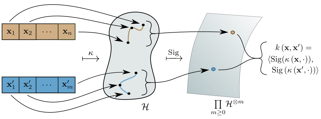
Figure 1: Time-series embedding via the signature kernel $k$ with static kernel $\kappa$. The time-series $\mathbf{x}$, $\tilde{\mathbf{x}}$ are lifted to paths in feature space $\mathcal{H}$, via $\kappa$ and some interpolation scheme, before being mapped to a Hilbert space $\prod_{m\geq 0}\mathcal{H}^{\otimes m}$ of tensors via the signature.

2.3 Likelihood-free inference

Many approaches to likelihood-free inference (lfi) have been proposed. Among them, a common theme is approximation of the true likelihood function or posterior density. Abc (see Beaumont, 2019, for a recent review) is a family of methods in which samples from an approximate posterior are derived through forward simulation of the model, $\mathbf{x}\sim p(\mathbf{x}\mid\bm{\theta})$, in combination with a summary statistic $\mathbf{s}$ and distance function $D(\mathbf{s}(\mathbf{x}),\mathbf{s}(\mathbf{y}))$ capturing a meaningful discrepancy between simulated and real data. It can be seen as an instance of kernel density estimation since the induced likelihood approximation permits the expression

$$p(\mathbf{y}\mid\bm{\theta})\approx\frac{1}{Q}\sum_{i=1}^{Q}K_{\varepsilon}\left(D(\mathbf{s}(\mathbf{x}^{(i)}),\mathbf{s}(\mathbf{y}))\right)$$

where $\mathbf{x}^{(i)}\overset{iid}{\sim}p(\mathbf{x}\mid\bm{\theta})$ and $K_{\varepsilon}$, a kernel function with window $\varepsilon$, largely controls the quality of the approximation. In contrast, a number of methods for lfi entail constructing explicit models of the likelihood function or posterior density. An early example is synthetic likelihood (Wood, 2010), in which $p\left(\mathbf{s}\left(\mathbf{x}\right)\mid\bm{\theta}\right)$ is modelled as a multivariate Gaussian with mean and covariance estimated from $Q>1$ simulations at $\bm{\theta}$. More recent examples include neural likelihood estimation (nle) (Papamakarios et al., 2019) and neural posterior estimation (npe) (Greenberg et al., 2019), in which $p\left(\mathbf{s}\left(\mathbf{x}\right)\mid\bm{\theta}\right)$ and $p\left(\bm{\theta}\mid\mathbf{s}\left(\mathbf{x}\right)\right)$, respectively, are estimated with highly flexible neural conditional density estimators, in particular normalising flows.

2.4 Amortised density ratio estimation

We briefly recapitulate dre for lfi, first introduced by Thomas et al. (2016), to estimate the likelihood-to-evidence ratio

$$r\left(\mathbf{x},\bm{\theta}\right)=\frac{p\left(\mathbf{x}\mid\bm{\theta}\right)}{p(\mathbf{x})}$$

and thus the parameter posterior $p\left(\bm{\theta}\mid\mathbf{x}\right)$ given a prior distribution $p\left(\bm{\theta}\right)$. Most relevant for us is amortised dre (Hermans et al., 2020). The core idea is to train a binary classifier to distinguish between positive examples $\left(\mathbf{x},\bm{\theta}\right)\sim p\left(\mathbf{x}\mid\bm{\theta}\right)p\left(\bm{\theta}\right)$ with label $z=1$ and negative examples $\left(\mathbf{x},\bm{\theta}\right)\sim p\left(\mathbf{x}\right)p\left(\bm{\theta}\right)$ with label $z=0$. The optimal decision boundary is then

$$d\left(\mathbf{x},\bm{\theta}\right)=\frac{p\left(\mathbf{x},\bm{\theta}\right)}{p\left(\mathbf{x},\bm{\theta}\right)+p\left(\mathbf{x}\right)p\left(\bm{\theta}\right)},$$ (4)

permitting posterior density evaluations as

$$p\left(\bm{\theta}\mid\mathbf{x}\right)=\frac{d\left(\mathbf{x},\bm{\theta}\right)}{1-d\left(\mathbf{x},\bm{\theta}\right)}p\left(\bm{\theta}\right)=r\left(\mathbf{x},\bm{\theta}\right)p\left(\bm{\theta}\right).$$ (5)

In practice, only an approximation $\hat{r}\left(\mathbf{x},\bm{\theta}\right)$ is available. Such approximations can be used for posterior sampling with Markov chain Monte Carlo (mcmc) (Pham et al., 2014; Thomas et al., 2016; Hermans et al., 2020, e.g.) or to perform likelihood ratio tests for frequentist inference (Cranmer et al., 2015; Dalmasso et al., 2020). As with neural likelihood and posterior estimation, we say that dre– in the form suggested by Hermans et al. (2020) – can be amortised since $\hat{r}\left(\mathbf{y},\bm{\theta}\right)$ can be evaluated for any observation $\mathbf{y}$ and any parameter $\bm{\theta}$ without retraining the density estimator.

2.5 Summary statistics

For many lfi methods, it is typically necessary to reduce high-dimensional data $\mathbf{x}$ into summary statistics $\mathbf{s}\left(\mathbf{x}\right)$. A number of approaches for doing so have been explored for abc, including semi-automatic abc (Fearnhead and Prangle, 2012), in which summary statistics $\mathbf{s}\left(\mathbf{y}\right)=\mathbb{E}\left[\bm{\theta}\mid\mathbf{y}\right]$ are estimated by performing a vector-valued regression of $\bm{\theta}^{(i)}$ onto $g\left(\mathbf{x}^{(i)}\right)$ for training data $\{{\left(\mathbf{x}^{(i)},\bm{\theta}^{(i)}\right)\}}_{i=1}^{Q}\sim p\left(\mathbf{x},\bm{\theta}\right)$ and candidate summary statistics $g\left(\cdot\right)$, and summary-free automatic methods which compute distances on the full dataset without the need to first compute summary statistics (Park et al., 2016; Bernton et al., 2019; Dyer et al., 2021a). More recently, Chen et al. (2020) explored the possibility of learning approximately sufficient, mutual information-maximising summary statistics with neural networks.

Some of these methods remain applicable to npe and dre. For example, Dinev and Gutmann (2018) use a convolutional neural network to learn $\mathbf{s}\left(\mathbf{x}\right)=\mathbb{E}\left[\bm{\theta}\mid\mathbf{x}\right]$, which are then used as predictors in a logistic regression model for dre. Npe and dre are however particularly interesting in that they permit the concurrent learning of both summary statistics and densities/ratios by augmenting a classifier with an initial embedding network (Lueckmann et al., 2017). This composite summary-learning/posterior-estimating network is trained end-to-end on the same loss function, producing competitive results (Greenberg et al., 2019). However, learning relevant features/summary statistics from neural networks in scenarios where sampling budgets are prohibitively low can be challenging.

For later reference, we tabulate some of the key works involving learning summary statistics for time-series data in lfi settings. We list for each the adopted training scheme, the number of trainable parameters in each case (each involved neural networks), and the assumed simulation budgets in Table 1.

Table 1: Summary of network sizes and simulation budgets for summary statistic learning in previous works.

Authors	Learning method	Network size	Simulation budget
Jiang et al. (2017)	Posterior mean as summary	$\sim 3\times 10^{4}$	$10^{6}$
Lueckmann et al. (2017)	Embedding network	$\sim 2\times 10^{3}$	$5\times 10^{3}-2.5\times 10^{4}$
Dinev and Gutmann (2018)	Posterior mean as summary	8,422	$10^{5}$
Greenberg et al. (2019)	Embedding network	$\sim 3\times 10^{4}$	Between $10^{3}$ and $\sim 10^{4}$
Chen et al. (2020)	Mutual information maximisation	$\sim 1.5\times 10^{4}$	$10^{3}-10^{4}$
Dyer et al. (2021b)	Embedding network	$\sim 10^{4}$	$10^{3}-10^{4}$

3 METHOD

Our goal is to perform amortised density ratio estimation as described in Section 2.4 for expensive simulators/low simulation budgets. As we will see in experiments below, learning both summary statistics and a classifier can be challenging in such regimes. To ameliorate this, we propose to build a classifier that leverages the signature kernel, which defines a universal kernel for multivariate and possibly irregularly sampled sequential data. The core idea is that using the predefined features captured by the signature and made available by the signature kernel may yield a more reliable density ratio estimator in low-sample regimes than alternative methods for which summary statistics must be learned.

To construct a probabilistic binary classifier using the signature, we may use the fact that a third kernel $m$ on $\mathcal{S}_{n}(\mathcal{X})\times\bm{\Theta}$ can be composed given two kernels $k:\mathcal{S}_{n}(\mathcal{X})\times\mathcal{S}_{n}(\mathcal{X})\to\mathbb{R}$ and $l:\bm{\Theta}\times\bm{\Theta}\to\mathbb{R}$ as

$$m\left(\left(\mathbf{x},\bm{\theta}\right),(\tilde{\mathbf{x}},\tilde{\bm{\theta}})\right)=k\left(\mathbf{x},\tilde{\mathbf{x}}\right)l(\bm{\theta},\tilde{\bm{\theta}}).$$ (6)

Taking $k$ to be the signature kernel (3) and $l$ to be a standard universal kernel on $\bm{\Theta}$, we may construct a kernel-based binary classifier for the purpose of performing dre for expensive time-series simulators, in this sense bypassing the need to learn summary statistics in addition to a density (ratio) estimator.

For a regularisation constant $\omega\in\mathbb{R}_{+}$, training a kernel binary classifier with loss $\ell$ amounts to solving the optimisation problem

$$\min_{f\in\mathcal{H}_{m}}\sum_{i=1}^{N}\ell\left(f(\mathbf{x}^{(i)},\bm{\theta}^{(i)}),z_{i}\right)+\frac{\omega}{2}\|f\|^{2}_{\mathcal{H}_{m}},$$ (7)

where $\mathcal{H}_{m}$ is the rkhs associated with $m$ and $z_{i}$ is the class label associated with data $(\mathbf{x}^{(i)},\bm{\theta}^{(i)})$. By the representer theorem, the solution to (7) is of the form

$$f\left(\mathbf{x},\bm{\theta}\right)=\sum_{i=1}^{N}c_{i}k\left(\mathbf{x}^{(i)},\mathbf{x}\right)l\left(\bm{\theta}^{(i)},\bm{\theta}\right)$$ (8)

for real coefficients $c_{i}$. Throughout, we use the logistic loss as $\ell$, since this is known to yield classifiers with well-calibrated probability estimates. This approach to learning the likelihood-to-evidence ratio is appealing since $m$ is a universal kernel:

Proposition 3.1.

Let $\mathcal{H}$ be a Hilbert space, $\mathcal{K}$ a compact set of continuous $\mathcal{H}$-valued paths of bounded variation on $\left[0,T\right]$, and assume that $\forall X\in\mathcal{K}$, $X$ has at least one monotone coordinate and $X(0)=\text{constant}$. Also let $k:\mathcal{K}\times\mathcal{K}\to\mathbb{R}$ be the signature kernel and $l$ be a universal kernel on $\bm{\Theta}$. Then $m$ as defined in Equation (6) is a universal kernel on $\mathcal{K}\times\bm{\Theta}$.

Proof.

From Kiŕaly and Oberhauser (2019, Theorem 1), the signature kernel is a universal kernel on $\mathcal{K}$. Then the assumed universality of $l$ and Blanchard et al. (2011, Lemma 5.2) give the desired result. ∎

The universality of $m$ then enables us to learn an estimate of the density ratio arbitrarily well.

3.1 Low-rank approximation

Computing the signature kernel for all pairs $\left(\mathbf{x}^{(i)},\mathbf{x}^{(j)}\right)$ in the simulated dataset can be expensive if the $\mathbf{x}^{(i)}$ are long and/or are high-dimensional. We therefore use the kernel $m$ defined in (6) – with $k$ the signature kernel and $l:\bm{\Theta}\times\bm{\Theta}\to\mathbb{R}$ an anisotropic Gaussian radial basis function (RBF) kernel – and the Nyström approximation to first find a representation of each pair $\left(\mathbf{x},\bm{\theta}\right)$ before feeding this low-dimensional approximation into the logistic regression model. For a given kernel $m$, the Nyström method (Williams and Seeger, 2001; Yang et al., 2012) provides a low-dimensional approximation $\hat{\phi}$ of the high- or potentially infinite-dimensional feature map $\phi(v):=m\left(v,\cdot\right)$ as follows: assume the kernel $m$ is of rank $q$ such that for any data $\{{v^{(i)}\}}_{i=1}^{N}$ we may write the corresponding Gram matrix $\mathbf{K}$ as

$$\mathbf{K}=\mathbf{U}\mathbf{D}\mathbf{U}^{\prime},$$ (9)

where $\mathbf{U}\in\mathbb{R}^{N\times q}$ is the matrix of eigenvectors and $\mathbf{D}=\mathrm{diag}\left(\lambda_{1},\dots,\lambda_{q}\right)\in\mathbb{R}^{q\times q}$ is the diagonal matrix consisting of eigenvalues $\lambda_{i}$. Then denoting the first $q$ rows of $\mathbf{U}$ as $\mathbf{U}_{q}$, we may find an approximate feature representation of $v$ under $m$ as Yang et al. (2012)

$$\hat{\phi}\left(v\right)=\mathbf{D}^{-\frac{1}{2}}\mathbf{U}_{q}^{\prime}\left[m\left(v,v^{(1)}\right),\dots,m\left(v,v^{(q)}\right)\right]^{\prime}.$$

Using these approximate feature representations obtained with the Nyström approximation, we then construct a linear logistic regression model by solving the following optimisation problem:

$$\min_{\mathbf{w}\in\mathbb{R}^{q}}\sum_{i=1}^{N}\ell\left(\mathbf{w}^{\prime}\hat{\phi}\left(v^{(i)}\right),z_{i}\right)+\frac{\omega}{2}\|\mathbf{w}\|^{2}_{2},$$ (10)

where $\ell$ is the logistic loss. We omit the use of an intercept in the linear logistic regression optimisation problem above for simplicity, but include it in practice.

Throughout the rest of this paper, we term this approach to performing ratio estimation with the signature kernel and logistic regression SignatuRE.

4 EXPERIMENTS

In this section, we present experiments on the relative performance of the SignatuRE method against possible alternatives for dre in likelihood-free inference contexts. For each task, we compare the quality of the posterior estimated with SignatuRE against the posteriors estimated with three alternatives:

1. a neural network consisting of a gated-recurrent unit (GRU) and residual network (ResNet), jointly termed GRU-ResNet. The GRU has trainable parameters $\varphi$ and consists of two stacked GRU layers of size 32. The GRU and ResNet are trained concurrently on the cross-entropy loss, so that the GRU learns a low-dimensional summary $\mathbf{s}_{\varphi}\left(\mathbf{x}\right)$ as the ResNet learns the density ratio;

2. a ResNet which instead consumes predefined, hand-crafted summary statistics $\tilde{\mathbf{s}}(\mathbf{x})$ that are tailored to the inference task and known to be informative of the parameters to be inferred for tractable simulation models, or that are commonly used elsewhere in the literature when the simulation model is not tractable. Such an approach should be considered a gold standard that is not generally available for complex, opaque simulation models whose structure cannot be exploited to derive suitable summary statistics. We refer to this method as the Bespoke ResNet;

3. ratio estimation with double kernel logistic regression (K2-RE), a modification of K2-ABC (Park et al., 2016) that we propose as an alternative kernel-based method for dre. The setup is identical to SignatuRE with the exception that, instead of the signature kernel, we use

   $$k\left(\mathbf{x},\tilde{\mathbf{x}}\right)=\exp\left(-\frac{\widehat{\textsc{MMD}}^{2}\left(\mu_{\mathbf{x}},\mu_{\tilde{\mathbf{x}}}\right)}{\epsilon}\right)$$ (11)

   as the positive definite kernel on $\mathbf{x}$, where $\mu_{\mathbf{x}}$ is the empirical measure consisting of the $n_{\mathbf{x}}$ points comprising $\mathbf{x}$ and $\widehat{\text{MMD}}^{2}\left(\mu_{\mathbf{x}},\mu_{\tilde{\mathbf{x}}}\right)$ is an unbiased estimate of the kernel maximum mean discrepancy between $\mu_{\mathbf{x}}$ and $\mu_{\tilde{\mathbf{x}}}$ for an appropriate kernel $\chi$ (see Section 3. Park et al., 2016). We use a Gaussian RBF and the median heuristic (Section 4. Park et al., 2016) for $\chi$. We include further details on this method in the supplement.

For the static kernel $\kappa$ in the signature kernel (see Section 2.1), we use a Gaussian RBF kernel with scale parameter chosen as $\mathrm{median}\{\|\mathbf{y}_{i}-\mathbf{y}_{j}\|^{2}_{i,j}\}$, where $\mathbf{y}=\left(\mathbf{y}_{1},\dots,\mathbf{y}_{n}\right)$ is the observation. For the kernel $l:\bm{\Theta}\times\bm{\Theta}\to\mathbb{R}$, we use an anisotropic Gaussian RBF kernel. To tune the length scale hyperparameters for $l$, the regularisation parameter $\omega$, and the $\epsilon$ parameter for K2-RE, we use Bayesian optimisation and 5-fold cross-validation (see the Supplementary Material for further details). To train the logistic regression models, we use the l-bfgs algorithm (Zhu et al., 1997) with a maximum number of 500 iterations.

To construct the set of negative examples $\left(\mathbf{x},\bm{\theta}\right)\sim p\left(\mathbf{x}\right)p\left(\bm{\theta}\right)$ for SignatuRE and K2-RE, we choose a proportion $K>0$ of the $\mathbf{x}^{(i)}$ and pair them with some $\bm{\theta}^{(j)}$, $j\neq i$. $K>1$ may also be chosen, in which case some $\mathbf{x}^{(i)}$ will appear multiple times in the set of negative examples. Unless stated otherwise, we take $K=1$ and $q=B_{\rm min}(K+1)$ in the Nyström approximation for both SignatuRE and K2-RE, where $B_{\rm min}$ is the smallest simulation budget considered in the experiment.

4.1 Computational expense

Evaluation of the signature kernel has complexity linear in the dimension of the time-series and linear (resp. quadratic) in the length of the time-series when evaluated on CPU (resp. GPU). Empirically, we observe SignatuRE to entail a comparable computational cost to the GRU-ResNet, the former typically requiring 3-5 CPU hours for training and inference and the latter typically requiring 1-2 CPU hours. For the simulation models for which we suppose our approach may be most helpful – those with significantly limited simulation budgets – we expect this to amount to a negligible difference: 1-4 additional CPU hours would allow for few or no additional simulations to be generated.

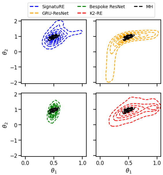
Figure 2: (Ornstein-Uhlenbeck) Posteriors obtained with SignatuRE (blue, top left), GRU-ResNet (orange, top right), Bespoke ResNet (green, bottom left), and K2-RE (red, bottom right) for a budget of 500 simulations and the approximate ground truth posterior obtained using the true likelihood function and Metropolis-Hastings (black).

4.2 Ornstein-Uhlenbeck process

The Ornstein-Uhlenbeck (ou) process (Uhlenbeck and Ornstein, 1930) is a prototypical Gauss–Markov stochastic differential equation (sde) model. We discretise the sde such that the data $\mathbf{x}=\left(\mathbf{x}_{0},\mathbf{x}_{1},\dots,\mathbf{x}_{T}\right),\mathbf{x}_{i}\in\mathbb{R}$ is generated according to

$$\mathbf{x}_{i}=\theta_{1}\exp{(\theta_{2})}\Delta t+(1-\theta_{1}\Delta t)\mathbf{x}_{i-1}+\frac{\epsilon_{i}}{2},$$

where $\Delta t=0.2$ is the time discretisation, $\bm{\theta}=\left(\theta_{1},\theta_{2}\right)$ are the model parameters to be inferred, $T=50$, and $\epsilon_{i}\sim\mathcal{N}\left(0,\Delta t\right)$. We generate $\mathbf{x}^{*}\sim p\left(\mathbf{x}\mid\bm{\theta}^{*}\right)$ with $\bm{\theta}^{*}=\left(0.5,1\right)$ and consider the task of estimating $p\left(\bm{\theta}\mid\mathbf{x}^{*}\right)$ given priors $\theta_{1}\sim\mathcal{U}\left(0,1\right)$ and $\theta_{2}\sim\mathcal{U}\left(-2,2\right)$.

We compare SignatuRE against the alternative dre methods described in Section 4. As $\tilde{\mathbf{s}}\left(\mathbf{x}\right)$, we use the intercept and slope of a linear regression of $\mathbf{x}_{t}$ vs. $\mathbf{x}_{t-1}$ as estimated with least squares (i.e. the maximum likelihood estimate) and the mean value of $\mathbf{x}$. These estimate $\theta_{1}\exp{(\theta_{2})}\Delta t$, $1-\theta_{1}\Delta t$, and $\exp\left(\theta_{2}\right)$, respectively, and are thus informative summary statistics for $\bm{\theta}$. For GRU-ResNet, we apply a linear layer of size 3 after the GRU in order to match the dimension of $\tilde{\mathbf{s}}$, resulting in a GRU with 9,795 trainable parameters.

In Figure 2 we show contour plots obtained by pooling the samples obtained from each ratio estimation method with a simulation budget of 500 simulations across 20 different seeds. Samples from the approximate ground truth posterior, obtained with Metropolis–Hastings (mh) (see Appendix for details) and the true likelihood function, are shown with black contour lines throughout. Additionally, we show in Figure 3 the Wasserstein distances (wd) between the estimated posteriors and the approximate ground truth posterior, and in Figure 4 the distances between the means of the estimated and approximate ground truth posteriors, for each ratio estimation method.

From this, we observe that GRU-ResNet (orange, top right of Figure 2) failed to learn both informative summary statistics and an accurate ratio estimator with a low simulation budget, despite the simplicity of the model. In contrast, an identical residual network used for Bespoke ResNet (green, bottom left of Figure 2) was able to learn a good estimate of the density ratio, even from such a limited simulation budget and with a summary statistic vector of identical size, but with the key difference that the summary statistics were predefined and designed to be informative of the parameter values being inferred.

This may be seen as an ablation study and suggests that the additional problem of learning summary statistics is the primary contributing factor to the relatively poor performance of GRU-ResNet.

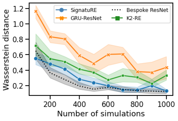
Figure 3: (Ornstein-Uhlenbeck) Wasserstein distances (mean + 95% confidence intervals) between posteriors obtained with each density ratio estimation method and the approximate ground truth posterior.

We also observe that, of the methods that do not use hand-crafted summary statistics, SignatuRE tends to exhibit superior performance. This is apparent from the posterior plots in Figure 2, and from Figure 3 in which SignatuRE consistently generates smaller wd s than GRU-ResNet and K2-RE and lags only slightly behind Bespoke ResNet.

From Figure 4 we see that SignatuRE tends to generate a significantly better parameter point estimate than GRU-ResNet and is additionally a slight improvement on K2-RE in this respect. The latter indicates that the success of SignatuRE in the low-simulation-budget regime is not only attributable to the expressive, preexisting feature representations available with general kernel methods, but also to the fact that the sequentialisation of the kernel employed in SignatuRE captures important information on the time-dependence of the data whereas in K2-RE the data is treated as iid.

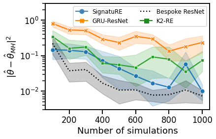
Figure 4: (Ornstein-Uhlenbeck) Euclidean distances (mean + 95% confidence intervals) between posterior means obtained with each density ratio estimation method and the approximate ground truth posterior.

4.3 Moving average model

We next consider a simple moving average model of order 2 (ma2), for which the data-generating process given parameters $\bm{\theta}=\left(\theta_{1},\theta_{2}\right)$ is

$$\mathbf{x}_{t}=\epsilon_{t}+\theta_{1}\epsilon_{t-1}+\theta_{2}\epsilon_{t-2},\ \ \epsilon_{t}\sim\mathcal{N}\left(0,1\right).$$ (12)

We generate $\mathbf{x}^{*}\sim p\left(\mathbf{x}\mid\bm{\theta}^{*}\right)$ with $\bm{\theta}^{*}=\left(0.6,0.2\right)$ and consider the task of estimating $p\left(\bm{\theta}\mid\mathbf{x}^{*}\right)$ given a uniform prior over the triangle given by $\theta_{1}+\theta_{2}>-1$, $\theta_{1}-\theta_{2}<1$, and $\theta_{2}<1$. Such a prior ensures that the model parameters are identifiable (Marin et al., 2012). Here, $\mathbf{x}$ and $\mathbf{x}^{*}$ are taken to be of length 50.

As $\tilde{\mathbf{s}}(\mathbf{x})$ we use the variance of the observed stream and the autocorrelations for lags 1 and 2. These give estimates of

$$\text{Var}\left(\mathbf{X}\right)=1\,+ \ \theta_{1}^{2}+\theta_{2}^{2},\ \ \ \rho_{1}=\frac{\theta_{1}+\theta_{1}\theta_{2}}{1+\theta_{1}^{2}+\theta_{2}^{2}},$$

and $$\rho_{2}=\frac{\theta_{2}}{1+\theta_{1}^{2}+\theta_{2}^{2}},$$

respectively, and are thus informative about $\bm{\theta}$. We once again apply a single linear layer of size 3 following the GRU in GRU-ResNet to match the dimensions of the summary statistics in Bespoke ResNet.

We show in Figure 5 the wd s between samples from the posteriors estimated with each density ratio estimation method and the approximate ground truth posterior obtained with Metropolis-Hastings mcmc. In Figure 6, we show the Euclidean distances between the means of the posteriors estimated with the different density ratio estimators and the approximate ground truth posterior. In this experiment, we once more see that Bespoke ResNet significantly outperforms GRU-ResNet in estimating the shape of the posterior distribution, despite the fact that they use identical residual networks to perform the density ratio estimation and that $\text{dim}\left(\tilde{\mathbf{s}}\right)=\text{dim}\left(\mathbf{s}_{\varphi}\right)$. This again suggests that the complex task of learning summary statistics in addition to learning the density ratio is the source of the difference in their performance.

We further observe that SignatuRE outperforms GRU-ResNet both in terms of the wd and distances between the estimated and approximate ground truth posterior means for simulation budgets of less than 500. For simulation budgets of 600-1000, SignatuRE and GRU-ResNet display comparable performance according to the wd s, while SignatuRE continues to obtain superior posterior mean estimates. Interestingly, SignatuRE additionally yields better estimates of the posterior mean than Bespoke ResNet, despite the fact that this density estimator has a considerable advantage through the use of hand-crafted summary statistics that are known to be informative of the parameters being inferred. As in the previous experiment, the success of SignatuRE appears to be attributable not only to the general properties of kernel methods that make them appealing in low-sample regimes – their ready-made, expressive feature spaces – but also to the fact that the signature accounts for the ordering of observations. We believe this explains the gap in performance between K2-RE and SignatuRE despite the former also being a kernel method.

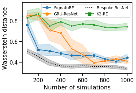
Figure 5: (MA(2)) Wasserstein distances (mean + 95% confidence intervals) between posteriors obtained with each density ratio estimation method and the approximate ground truth posterior.

4.4 Complex, intractable example: partially-observed stochastic epidemic

Finally, we consider a more complex example with an intractable posterior distribution. The model we consider here is a generalised stochastic epidemic (gse) model (Kypraios, 2007), which simulates the spread of an infection through a fixed population of $N$ individuals. Individuals in the system are initially susceptible, can become infected, and subsequently enter a recovered state in which they are no longer susceptible to reinfection. In a time interval $\delta t$, infections, recoveries, and an absence of activity occur with probabilities

$${}P_{I}:=P\left[(\delta X_{t},\delta Y_{t})=(-1,1)\mid\sigma_{t}\right]=\beta X_{t}Y_{t}\delta t+o(\delta t),$$

$${}P_{R}:=P\left[(\delta X_{t},\delta Y_{t})=(0,-1)\mid\sigma_{t}\right]=\gamma Y_{t}\delta t+o(\delta t),$$

$${}P\left[(\delta X_{t},\delta Y_{t})=(0,0)\mid\sigma_{t}\right]=1-(P_{I}+P_{R}),$$

respectively, where $X_{t}$ and $Y_{t}$ are the number of susceptible and infected agents at time $t\in[0,T]$, respectively, $\sigma_{t}$ is a sigma-algebra generated by the process up until time $t$, and $\bm{\theta}=\left(\beta,\gamma\right)$ is the model parameter.

We simulate the model using the Gillespie algorithm (Gillespie, 1977) and observe the series $\mathbf{x}=\left(X_{i\Delta t},Y_{i\Delta t}\right)_{i=0}^{D}\in\mathcal{S}_{D+1}\left(\mathbb{R}^{2}\right)$ at regular time intervals of length $\Delta t=0.5$ with $D=100$. We consider the task of estimating $p\left(\bm{\theta}\mid\mathbf{x}^{*}\right)$ for $\mathbf{x}^{*}\sim p\left(\mathbf{x}\mid\bm{\theta}^{*}\right)$, $\bm{\theta}^{*}=\left(10^{-2},10^{-1}\right)$, and priors $\beta\sim\Gamma\left(0.1,2\right)$ and $\gamma\sim\Gamma\left(0.2,0.5\right)$. To sample from the posterior in this case, we use a sampling importance resampling (sir) scheme: we sample $\mathcal{T}=\{{\bm{\theta}_{m}\}}_{m=1}^{M}$ from the prior, before resampling $\{{\tilde{\bm{\theta}}_{m}\}}_{m=1}^{\tilde{M}}$ from $\mathcal{T}$, where each sample in $\mathcal{T}$ has weight proportional to the density ratio estimated by the classifiers. We take $M=5\times 10^{4}$ and $\tilde{M}=10^{3}$.

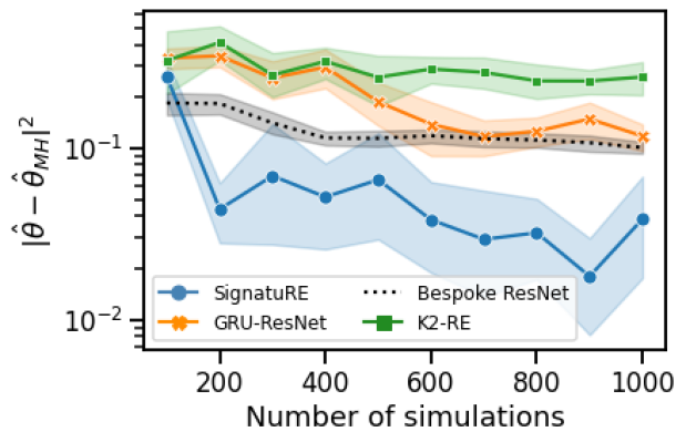
Figure 6: (MA(2)) Euclidean distances (mean + 95% confidence intervals) between posterior means obtained with each density ratio estimation method and the approximate ground truth posterior mean.

Table 2: Median Wasserstein distance from smc-abc posterior for the partially-observed epidemic model (from 10 seeds). Smaller values are better. Bold and italics indicate best and second-best, respectively, of the methods that do not use pre-defined summary statistics.

Method	Simulation budget
	50	100	200	500	1000
GRU-ResNet	0.434	0.425	0.355	0.273	0.090
K2-RE	0.417	0.432	0.407	0.454	0.431
K2-RE-5	0.440	0.427	0.374	0.206	0.255
SignatuRE	0.430	0.411	0.351	0.513	0.321
SignatuRE-5	0.241	0.333	0.176	0.133	0.083
Bespoke ResNet	0.379	0.222	0.146	0.104	0.092

In this instance, the ground truth posterior distribution is not available for comparison. For this reason, we assess the quality of inferences by comparing against the posterior obtained from sequential Monte Carlo abc (smc-abc) (Beaumont et al., 2009) in which we use the Euclidean distance between time-series

$$\sum_{i=0}^{D}\|\mathbf{x}_{i}-\mathbf{x}^{*}_{i}\|^{2}_{2}$$ (13)

as the distance measure with $10^{7}$ simulations, a Gaussian kernel, and $\epsilon$ decay factor equal to 0.8. We again compare SignatuRE with GRU-ResNet, Bespoke ResNet, and K2-RE. For Bespoke ResNet, we use the mean of each series, log variance of each series, autocorrelation coefficients for lags 1 and 2 of each series, and the cross-correlation coefficient between the two series as $\tilde{\mathbf{s}}(\mathbf{x})$, which are common summary statistics for stochastic kinetic models (Papamakarios et al., 2019; Greenberg et al., 2019). For GRU-ResNet, we apply a single linear layer of size 9 to match the dimensions of $\tilde{\mathbf{s}}(\mathbf{x})$.

We present the median Wasserstein distance between the estimated posteriors and the approximate ground truth posterior from smc-abc in Table 2, in which suffix “-5” indicates that $K=5$ for kernel methods (otherwise $K=1$ is used as before). We take $q=B_{\rm min}(K+1)$ components in the Nyström approximation for both SignatuRE and K2-RE, where $B_{\rm min}=50$ is the minimum simulation budget in this experiment. Median values are obtained by repeating the inference procedure over 10 different random seeds using the same pseudo-observed data. Of the methods that must learn summary statistics (i.e. all but Bespoke ResNet), our methods are either best (bold) or second-best (italics) for all budgets, but the improvement in performance over GRU-ResNet at a budget of 1000 simulations is minor. While this demonstrates that the range of applicability of SignatuRE may be limited, it nonetheless also demonstrates that SignatuRE can be preferable under extreme restrictions on the simulation budget, as can be the case in many real-world contexts.

5 DISCUSSION

This paper discusses the use of signature transforms as automatic and effective feature extractors for likelihood (ratio) estimation. Our method, based on universal kernels for sequential data and termed SignatuRE, delivers competitive performance even when sample numbers are very low. Indeed, our simulation studies suggest that using signatures as features improves upon a time-series specialised GRU-ResNet or kernels based on maximum mean discrepancies in low-simulation-budget scenarios. We propose that this can be understood in the following way: while GRU-ResNet must learn adequate summary statistics – which can be difficult for low simulation budgets – and K2-RE uses a kernel maximum mean discrepancy estimator that treats the points in the time-series as exchangeable, destroying important dependencies, SignatuRE uses expressive ready-made geometric features for paths which take the ordering of points into account. In our experiments, SignatuRE was only consistently outperformed by a classifier that used bespoke hand-crafted summary statistics which were constructed by carefully inspecting the model structure. For real, complex simulators, such an approach is infeasible, making the proposed method appealing.

Acknowledgements

The authors thank Harald Oberhauser and the anonymous reviewers for their helpful feedback. JD is supported by the EPSRC Centre For Doctoral Training in Industrially Focused Mathematical Modelling (EP/L015803/1) in collaboration with Improbable.

 

Supplementary Material:
Amortised Likelihood-free Inference for Expensive Time-series Simulators with Signatured Ratio Estimation

 

Appendix A EXPERIMENT DETAILS

A.1 Further details on K2-RE

To test the hypothesis that the signature kernel is responsible for the improved performance seen in the experiments presented in the main text, we construct and compare an alternative kernel-based classifier to compare against. The design of this classifier is chosen to match exactly that of SignatuRE, with an important change: the kernel $k$ is no longer taken to be the signature kernel, but instead a kernel based on the K2-ABC (Park et al., 2016):

$$k\left(\mathbf{x},\tilde{\mathbf{x}}\right)=\exp\left(-\frac{\widehat{\textsc{MMD}}^{2}\left(\mu_{\mathbf{x}},\mu_{\tilde{\mathbf{x}}}\right)}{\epsilon}\right),$$ (14)

where

$$\widehat{\textsc{MMD}}^{2}\left(\mu_{\mathbf{x}},\mu_{\tilde{\mathbf{x}}}\right)=-\frac{2}{n_{\mathbf{x}}n_{\tilde{\mathbf{x}}}}\sum_{i=1}^{n_{\mathbf{x}}}\sum_{j=1}^{n_{\tilde{\mathbf{x}}}}\chi\left(\mathbf{x}_{i},\tilde{\mathbf{x}}_{j}\right)+\frac{1}{n_{\mathbf{x}}\left(n_{\mathbf{x}}-1\right)}\sum_{\begin{subarray}{c}i=1\end{subarray}}^{n_{\mathbf{x}}}\sum_{\begin{subarray}{c}j\neq i\end{subarray}}\chi\left(\mathbf{x}_{i},\mathbf{x}_{j}\right)\\ +\frac{1}{n_{\tilde{\mathbf{x}}}\left(n_{\tilde{\mathbf{x}}}-1\right)}\sum_{\begin{subarray}{c}i=1\end{subarray}}^{n_{\tilde{\mathbf{x}}}}\sum_{\begin{subarray}{c}j\neq i\end{subarray}}\chi\left(\tilde{\mathbf{x}}_{i},\tilde{\mathbf{x}}_{j}\right)$$ (15)

is an unbiased estimate of the kernel maximum mean discrepancy between measures $\mu_{\mathbf{x}}$ and $\mu_{\tilde{\mathbf{x}}}$ for an appropriate kernel $\chi$ (see Section 3. Park et al., 2016). We use a Gaussian RBF and the median heuristic (Section 4. Park et al., 2016) for $\chi$.

Comparing against an alternative kernel classifier that does not account for the ordering of the points $\mathbf{x}_{i}$ in $\mathbf{x}$ allows us to test the hypothesis that it is specifically the signature kernel, and not just kernel methods in general, that allow us to achieve the improved performance at low simulation budgets.

A.2 Tuning kernel parameters

To optimise the kernel parameters for SignatuRE and K2-RE, we use 5-fold cross-validation and Bayesian optimisation via a tree Parzen estimator with the following priors:

1. a log-uniform prior with bounds $\left[\log{10^{-3}},\log{10^{3}}\right]$ for all lengthscale parameters;

2. a log-uniform prior with bounds $\left[\log{10^{-5}},\log{10^{4}}\right]$ for the regularisation parameters.

For this purpose, we make use of the hyperopt python package (Bergstra et al., 2013).

A.3 Training the ResNet models

For both GRU-ResNet and Bespoke ResNet, the ResNet consists of two hidden layers of 50 units with ReLU activations, which has previously been seen to produce state-of-the-art performance in likelihood-free density ratio estimation tasks (Durkan et al., 2020; Lueckmann et al., 2017). We follow Durkan et al. (2020) and use Adam (Kingma and Ba, 2014) to train the network weights, along with a training batch size of 50 and learning rate of $5\times 10^{-4}$. We furthermore reserve 10% of the data for validation, and stop training when the validation error does not improve over 20 epochs to avoid overfitting. For these density ratio estimators, we use the sbi python package (Tejero-Cantero et al., 2020).

A.4 Sampling with Metropolis-Hastings

Unless stated otherwise, we obtain samples from both the approximate ground-truth posteriors and the posterior distributions estimated with density ratios with Metropolis-Hastings Markov chain Monte Carlo. We use a normal proposal distribution $q(\tilde{\bm{\theta}}\mid\bm{\theta})=\mathcal{N}\left(\bm{\theta},\ell^{2}\Sigma\right)$ with covariance matrix $\Sigma$, which estimate by performing a trial run of 50,000 steps with a diagonal proposal covariance matrix (see e.g. the guidelines in Gelman et al., 2013, Section 12.2) and setting $\ell=2/\sqrt{d}$ for $\bm{\theta}\in\mathbb{R}^{d}$ (Roberts et al., 1997). This works well if the posterior is approximately normal (see Schmon and Gagnon, 2022). Once $\Sigma$ is estimated, we run one further chain for 100,000 steps, and thin by retaining every 100th sample. We furthermore start every chain from the true parameter values $\bm{\theta}^{*}$.

A.5 Confidence interval evaluations

In Figures 3-6 in the main text, the 95% confidence intervals are bootstrap confidence intervals obtained by running the training procedures at different seeds and subsequently applying the trained ratio estimators to the task of obtaining the posterior for the same pseudo-observed data in each case.

References

- Baptista et al. (2016) Rafa Baptista, J Doyne Farmer, Marc Hinterschweiger, Katie Low, Daniel Tang, and Arzu Uluc. Macroprudential policy in an agent-based model of the UK housing market. 2016.
- Beaumont (2019) Mark A Beaumont. Approximate Bayesian computation. Annual review of statistics and its application, 6:379–403, 2019.
- Beaumont et al. (2002) Mark A Beaumont, Wenyang Zhang, and David J Balding. Approximate Bayesian computation in population genetics. Genetics, 162(4):2025–2035, 2002.
- Beaumont et al. (2009) Mark A. Beaumont, Jean-Marie Cornuet, Jean-Michel Marin, and Christian P. Robert. Adaptive approximate bayesian computation. Biometrika, 96(4):983–990, 2009. ISSN 00063444, 14643510. URL http://www.jstor.org/stable/27798882.
- Bernton et al. (2019) Espen Bernton, Pierre E. Jacob, Mathieu Gerber, and Christian P. Robert. Approximate Bayesian computation with the Wasserstein distance. Journal of the Royal Statistical Society. Series B: Statistical Methodology, 81(2):235–269, 2019. ISSN 14679868. doi: 10.1111/rssb.12312.
- Blanchard et al. (2011) Gilles Blanchard, Gyemin Lee, and Clayton Scott. Generalizing from several related classification tasks to a new unlabeled sample. In Proceedings of the 24th International Conference on Neural Information Processing Systems, NIPS’11, page 2178–2186, Red Hook, NY, USA, 2011. Curran Associates Inc. ISBN 9781618395993.
- Chen et al. (2020) Yanzhi Chen, Dinghuai Zhang, Michael Gutmann, Aaron Courville, and Zhanxing Zhu. Neural Approximate Sufficient Statistics for Implicit Models. pages 1–14, 2020. URL http://arxiv.org/abs/2010.10079.
- Christensen et al. (2015) Kim Christensen, Kishan A. Manani, and Nicholas S. Peters. Simple model for identifying critical regions in atrial fibrillation. Physical Review Letters, 114(2):1–6, 2015. ISSN 10797114. doi: 10.1103/PhysRevLett.114.028104.
- Cranmer et al. (2015) Kyle Cranmer, Juan Pavez, and Gilles Louppe. Approximating likelihood ratios with calibrated discriminative classifiers. arXiv preprint arXiv:1506.02169, 2015.
- Dalmasso et al. (2020) Niccolo Dalmasso, Rafael Izbicki, and Ann Lee. Confidence sets and hypothesis testing in a likelihood-free inference setting. In Hal Daumé III and Aarti Singh, editors, Proceedings of the 37th International Conference on Machine Learning, volume 119 of Proceedings of Machine Learning Research, pages 2323–2334. PMLR, 13–18 Jul 2020. URL https://proceedings.mlr.press/v119/dalmasso20a.html.
- Danabasoglu et al. (2020) Gokhan Danabasoglu, J-F Lamarque, J Bacmeister, DA Bailey, AK DuVivier, Jim Edwards, LK Emmons, John Fasullo, R Garcia, Andrew Gettelman, et al. The community earth system model version 2 (cesm2). Journal of Advances in Modeling Earth Systems, 12(2), 2020.
- Diggle and Gratton (1984) Peter J Diggle and Richard J Gratton. Monte carlo methods of inference for implicit statistical models. Journal of the Royal Statistical Society: Series B (Methodological), 46(2):193–212, 1984.
- Dinev and Gutmann (2018) Traiko Dinev and Michael U. Gutmann. Dynamic Likelihood-free Inference via Ratio Estimation (DIRE), 2018.
- Durkan et al. (2020) Conor Durkan, Iain Murray, and George Papamakarios. On Contrastive Learning for Likelihood-free Inference. In Hal Daumé III and Aarti Singh, editors, Proceedings of the 37th International Conference on Machine Learning, volume 119 of Proceedings of Machine Learning Research, pages 2771–2781. PMLR, 13–18 Jul 2020. URL http://proceedings.mlr.press/v119/durkan20a.html.
- Dyer et al. (2021a) Joel Dyer, Patrick Cannon, and Sebastian M Schmon. Approximate Bayesian Computation with Path Signatures. arXiv preprint arXiv:2106.12555, 2021a.
- Dyer et al. (2021b) Joel Dyer, Patrick W Cannon, and Sebastian M Schmon. Deep Signature Statistics for Likelihood-free Time-series Models. In ICML Workshop on Invertible Neural Networks, Normalizing Flows, and Explicit Likelihood Models, 2021b.
- Dyer et al. (2022) Joel Dyer, Patrick Cannon, J. Doyne Farmer, and Sebastian M Schmon. Black-box Bayesian inference for economic agent-based models. arXiv preprint arXiv:2202.00625, 2022.
- Fearnhead and Prangle (2012) Paul Fearnhead and Dennis Prangle. Constructing summary statistics for approximate Bayesian computation: Semi-automatic approximate Bayesian computation. Journal of the Royal Statistical Society: Series B (Statistical Methodology), 74(3):419–474, 2012.
- Gelman et al. (2013) Andrew Gelman, John B Carlin, Hal S Stern, David B Dunson, Aki Vehtari, and Donald B Rubin. Bayesian data analysis. 2013.
- Gillespie (1977) Daniel T. Gillespie. Exact stochastic simulation of coupled chemical reactions. The Journal of Physical Chemistry, 81(25):2340–2361, 1977. doi: 10.1021/j100540a008. URL https://doi.org/10.1021/j100540a008.
- Greenberg et al. (2019) David S. Greenberg, Marcel Nonnenmacher, and Jakob H. Macke. Automatic posterior transformation for likelihood-free inference. 36th International Conference on Machine Learning, ICML 2019, 2019-June:4288–4304, 2019.
- Hambly and Lyons (2010) Ben Hambly and Terry Lyons. Uniqueness for the signature of a path of bounded variation and the reduced path group. Annals of Mathematics, 171(1):109–167, Mar 2010. ISSN 0003-486X. doi: 10.4007/annals.2010.171.109. URL http://dx.doi.org/10.4007/annals.2010.171.109.
- Hermans et al. (2020) Joeri Hermans, Volodimir Begy, and Gilles Louppe. Likelihood-free MCMC with amortized approximate ratio estimators. In International Conference on Machine Learning, pages 4239–4248. PMLR, 2020.
- Jagiella et al. (2017) Nick Jagiella, Dennis Rickert, Fabian J Theis, and Jan Hasenauer. Parallelization and high-performance computing enables automated statistical inference of multi-scale models. Cell systems, 4(2):194–206, 2017.
- Jiang et al. (2017) Bai Jiang, Tung-yu Wu, Charles Zheng, and Wing H Wong. Learning summary statistic for approximate bayesian computation via deep neural network. Statistica Sinica, pages 1595–1618, 2017.
- Kennedy and O’Hagan (2001) Marc C Kennedy and Anthony O’Hagan. Bayesian calibration of computer models. Journal of the Royal Statistical Society: Series B (Statistical Methodology), 63(3):425–464, 2001.
- Kingma and Ba (2014) Diederik P Kingma and Jimmy Ba. Adam: A method for stochastic optimization. arXiv preprint arXiv:1412.6980, 2014.
- Kiŕaly and Oberhauser (2019) Franz J. Kiŕaly and Harald Oberhauser. Kernels for sequentially ordered data. Journal of Machine Learning Research, 20, 2019. ISSN 15337928.
- Kypraios (2007) Theo Kypraios. Efficient bayesian inference for partially observed stochastic epidemics and a new class of semi-parametric time series models. 2007.
- Levin et al. (2016) Daniel Levin, Terry Lyons, and Hao Ni. Learning from the past, predicting the statistics for the future, learning an evolving system, 2016.
- Lueckmann et al. (2017) Jan-Matthis Lueckmann, Pedro J Goncalves, Giacomo Bassetto, Kaan Öcal, Marcel Nonnenmacher, and Jakob H Macke. Flexible statistical inference for mechanistic models of neural dynamics. In Advances in Neural Information Processing Systems, 2017.
- Lueckmann et al. (2021) Jan-Matthis Lueckmann, Jan Boelts, David Greenberg, Pedro Goncalves, and Jakob Macke. Benchmarking simulation-based inference. In Arindam Banerjee and Kenji Fukumizu, editors, Proceedings of The 24th International Conference on Artificial Intelligence and Statistics, volume 130 of Proceedings of Machine Learning Research, pages 343–351. PMLR, 13–15 Apr 2021.
- Lyons (2014) Terry Lyons. Rough paths, signatures and the modelling of functions on streams. arXiv preprint arXiv:1405.4537, 2014.
- Marin et al. (2012) Jean Michel Marin, Pierre Pudlo, Christian P. Robert, and Robin J. Ryder. Approximate Bayesian computational methods. Statistics and Computing, 22(6):1167–1180, 2012. ISSN 09603174. doi: 10.1007/s11222-011-9288-2.
- Papamakarios et al. (2019) George Papamakarios, David Sterratt, and Iain Murray. Sequential neural likelihood: Fast likelihood-free inference with autoregressive flows. In The 22nd International Conference on Artificial Intelligence and Statistics, pages 837–848. PMLR, 2019.
- Park et al. (2016) Mijung Park, Wittawat Jitkrittum, and Dino Sejdinovic. K2-ABC: Approximate bayesian computation with kernel embeddings. Proceedings of the 19th International Conference on Artificial Intelligence and Statistics, AISTATS 2016, 41:398–407, 2016.
- Pham et al. (2014) Kim Cuc Pham, David J Nott, and Sanjay Chaudhuri. A note on approximating abc-mcmc using flexible classifiers. Stat, 3(1):218–227, 2014.
- Pritchard et al. (1999) Jonathan K Pritchard, Mark T Seielstad, Anna Perez-Lezaun, and Marcus W Feldman. Population growth of human Y chromosomes: a study of Y chromosome microsatellites. Molecular biology and evolution, 16(12):1791–1798, 1999.
- Roberts et al. (1997) GO Roberts, A Gelman, and WR Gilks. Weak convergence and optimal scaling of random walk metropolis algorithms. The Annals of Applied Probability, pages 110–120, 1997.
- Salvi et al. (2021) Cristopher Salvi, Thomas Cass, James Foster, Terry Lyons, and Weixin Yang. The Signature Kernel Is the Solution of a Goursat PDE. SIAM Journal on Mathematics of Data Science, 3(3):873–899, 2021. doi: 10.1137/20M1366794. URL https://doi.org/10.1137/20M1366794.
- Schmon and Gagnon (2022) Sebastian M Schmon and Philippe Gagnon. Optimal scaling of random walk metropolis algorithms using bayesian large-sample asymptotics. Statistics and Computing, forthcoming, 2022.
- Shawe-Taylor and Cristianini (2004) John Shawe-Taylor and Nello Cristianini. Kernel Methods for Pattern Analysis. Cambridge University Press, 2004. doi: 10.1017/CBO9780511809682.
- Tejero-Cantero et al. (2020) Alvaro Tejero-Cantero, Jan Boelts, Michael Deistler, Jan-Matthis Lueckmann, Conor Durkan, Pedro J. Gonçalves, David S. Greenberg, and Jakob H. Macke. sbi: A toolkit for simulation-based inference. Journal of Open Source Software, 5(52):2505, 2020. doi: 10.21105/joss.02505. URL https://doi.org/10.21105/joss.02505.
- Thomas et al. (2016) Owen Thomas, Ritabrata Dutta, Jukka Corander, Samuel Kaski, and Michael U Gutmann. Likelihood-free inference by ratio estimation. arXiv preprint arXiv:1611.10242, 2016.
- Uhlenbeck and Ornstein (1930) G.E. Uhlenbeck and L.S. Ornstein. On the theory of the brownian motion. Physical Review, 36(5):823–841, 1930. ISSN 0031899X.
- Williams and Seeger (2001) Christopher Williams and Matthias Seeger. Using the nyström method to speed up kernel machines. In Proceedings of the 14th annual conference on neural information processing systems, number CONF, pages 682–688, 2001.
- Wood (2010) Simon N. Wood. Statistical inference for noisy nonlinear ecological dynamic systems. Nature, 466(7310):1102–1104, 2010. ISSN 00280836. doi: 10.1038/nature09319.
- Yang et al. (2012) Tianbao Yang, Yu-feng Li, Mehrdad Mahdavi, Rong Jin, and Zhi-Hua Zhou. Nyström method vs random fourier features: A theoretical and empirical comparison. In F. Pereira, C. J. C. Burges, L. Bottou, and K. Q. Weinberger, editors, Advances in Neural Information Processing Systems, volume 25. Curran Associates, Inc., 2012. URL https://proceedings.neurips.cc/paper/2012/file/621bf66ddb7c962aa0d22ac97d69b793-Paper.pdf.
- Zhu et al. (1997) Ciyou Zhu, Richard H. Byrd, Peihuang Lu, and Jorge Nocedal. Algorithm 778: L-BFGS-B: Fortran Subroutines for Large-Scale Bound-Constrained Optimization. ACM Trans. Math. Softw., 23(4):550–560, December 1997. ISSN 0098-3500. doi: 10.1145/279232.279236. URL https://doi.org/10.1145/279232.279236.