OU-HEP-220301

Mini-review: Expectations for supersymmetry
from the string landscape

 

 

Submitted to the Proceedings of the US Community Study

on the Future of Particle Physics (Snowmass 2021)

 

 

Howard Baer¹, Vernon Barger², Shadman Salam¹ and Dibyashree Sengupta^3
1Homer L. Dodge Department of Physics and Astronomy, University of Oklahoma, Norman, OK 73019, USA
²Department of Physics, University of Wisconsin, Madison, WI 53706 USA
³Department of Physics, National Taiwan University, Taipei, Taiwan 10617, R.O.C.

In this mini-review, we summarize a variety of findings pertaining to consequences of the landscape of string theory for supersymmetry (SUSY) phenomenology. The idea is to adopt the MSSM as the most parsimonious $4-d$ low energy EFT after string compactification but where the scale of SUSY breaking is as yet undetermined. A power-law landscape draw to large soft terms is tempered by the requirement that the derived value of the weak scale lie within the anthropic window of Agrawal et al. (ABDS). Such a set-up predicts a light Higgs mass $m_{h}\sim 125$ GeV with sparticles generally beyond LHC bounds. We discuss consequences for LHC searches: light higgsinos, highly mixed TeV-scale top squarks, same-sign diboson events and $m_{\tilde{g}}\sim 2-5$ TeV. We expect dark matter to consist of an axion/higgsino-like WIMP admixture.

1 Introduction and set up

So far, superstring theory provides our only successful unification of quantum mechanics with general relativity[1, 2]. However, to avoid anomalies, then the dimensionality of spacetime must be increased to ten (or even eleven in $M$-theory[3]). To gain accord with the $4-d$ physics of the Standard Model, one must compactify the extra six dimensions on a suitable compact manifold, such a Calabi-Yau (CY) manifold, which preserves $N=1$ supersymmetry in the low energy effective field theory (EFT)[4]. The $4-d$ laws of physics after compactification then depend on various properties of the compact manifold, which are parametrized by vacuum expectation values (vevs) of moduli fields: gravitationally interacting scalar fields with a flat classical potential. To gain a realistic and potentially predictive theory, the moduli must be stabilized so as to avoid runaway solutions and to gain well-determined vevs which in turn determine various low energy properties such as the values of gauge and Yukawa couplings and soft SUSY breaking terms[5].

At the turn of the 21st century, it was realized that the number of possibilities for compact CY manifolds was far, far greater than anticipated[6]. Under flux comactifications[7], the number of distinct vacuum states might range from $10^{500}$[8] to $10^{272,000}$[9]. These are more than enough to implement Weinberg’s anthropic solution to the cosmological constant (CC) problem[10]. It also provides a new understanding of how vastly different energy scales may emerge from string theory which contains only the string scale $m_{s}$ at its most fundamental level. In an eternally inflating multiverse[11, 12], different pocket universes can arise with different physical constants. Requiring a pocket universe to allow for large scale structure in the form of galaxies and clusters, then only those with a tiny cosmological constant are allowed. Indeed, this approach allowed Weinberg to predict the value of the cosmological constant to a factor of a few a decade before its tiny yet non-zero value was measured[10, 13].

A similar approach may be applied to the origin of the weak scale $m_{weak}\sim m_{W,Z,h}$ in models with weak scale supersymmetry[14] (WSS) (for a recent review of WSS after LHC Run 2, see Ref. [15]). In models such as the MSSM, the weak scale is determined by the soft SUSY breaking parameters and the SUSY conserving $\mu$ parameter. Minimizing the MSSM scalar (Higgs) potential, one finds

$$m_{Z}^{2}/2=\frac{m_{H_{d}}^{2}+\Sigma_{d}^{d}-(m_{H_{u}}^{2}+\Sigma_{u}^{u})\tan^{2}\beta}{\tan^{2}\beta-1}-\mu^{2}$$ (1)

Here, $m_{H_{u}}^{2}$ and $m_{H_{d}}^{2}$ are the weak scale values of the soft SUSY breaking Higgs masses, $\tan\beta\equiv v_{u}/v_{d}$ is the ratio of Higgs field vevs and the terms $\Sigma_{u}^{u}$ and $\Sigma_{d}^{d}$ contain over 40 loop corrections to the Higgs potential (for a tabulation, see Ref’s [17] and [18]). The largest of these typically come from the top squarks: $\Sigma_{u}^{u}(\tilde{t}_{1,2})$. Equation 1 allows for a definition of the weak scale finetuning measure $\Delta_{EW}\equiv|largest\ term\ on\ RHS\ |/(m_{Z}^{2}/2)$[19].

If we adopt a so-called fertile patch of the landscape– those vacua whose $4-d$ low energy EFT is, by parsimony, the MSSM– then we would expect the magnitude of the weak scale to vary in each pocket universe depending on the values of the soft breaking terms and $\mu$ parameter in that same pocket universe[20]. We can write the distribution of vacua versus the soft SUSY breaking scale $m_{soft}$ (where $m_{soft}\simeq m_{SUSY}^{2}/m_{P}$ in gravity mediation where $m_{SUSY}\sim 10^{11}$ GeV is the mass scale associated with hidden sector SUSY breaking) as

$$dN_{vac}\sim f_{SUSY}(m_{soft})\cdot f_{EWSB}(m_{soft})\cdot dm_{soft}.$$ (2)

Douglas and others[21, 22, 23] originally proposed that

$$f_{SUSY}\sim m_{soft}^{2n_{F}+n_{D}-1}$$ (3)

where $n_{F}$ is the number of $F$-term SUSY breaking fields and $n_{D}$ is the number of $D$-term SUSY breaking fields contributing to the overall SUSY breaking scale. The factor 2 arises since it is expected that the vevs $F_{i}$ are distributed uniformly as complex numbers whilst the $D_{j}$ are distributed uniformly as real numbers. It was realized shortly thereafter that this may be too simplistic in that the sources of SUSY breaking may not all be independent[24]. But even so, for the textbook case of spontaneous SUSY breaking by a single $F$-term, then already one expects soft terms to be statistically favored to large values by a linear distribution $f_{SUSY}\sim m_{soft}^{1}$. An alternative– emphasized by Dine et al.[25, 26]– is that SUSY is broken non-perturbatively in a hidden sector via e.g. dynamical SUSY breaking either via gaugino condensation or via instanton effects. In such a case, then no SUSY breaking scale is favored over any other, which would result in $f_{SUSY}\sim m_{soft}^{-1}$. These results have some further support from Broeckel et al.[27] where they investigate the statistics of SUSY breaking in the landscape including considerations of Kähler moduli ($T_{i}$) stabilization. For the large volume scenario (LVS)[28] where the $T_{i}$ are stabilized by a balance between perturbative and non-perturbative effects, then they find $f_{SUSY}\sim m_{soft}^{-1}$ while for non-perturbative Kähler moduli stabilization as in KKLT[29] they find $f_{SUSY}\sim m_{soft}^{1}$. Thus, in the following, we will compare statistical predictions from the string landscape assuming $f_{SUSY}\sim m_{soft}^{\pm 1}$.

The other relevant distribution contains (anthropic) selection effects in $f_{EWSB}$. Agrawal, Barr, Donoghue and Seckel (ABDS)[30, 31] showed already in 1997 that too large a value of the weak scale in various causally disconnected domains of the multiverse would lead, via the up-down quark mass difference, to unstable nuclei and lack of atoms which are apparently needed for life as we know it. They estimate that for pocket universes with $m_{weak}^{PU}\gtrsim(2-5)m_{weak}^{OU}$, then one is in violation of this so-called atomic principle (where $m_{weak}^{OU}$ corresponds to the magnitude of the weak scale in our universe). Without finetuning, then the pocket universe value of the weak scale corresponds to the maximal term on the RHS of Eq. 1. Then requiring for definiteness $m_{weak}^{PU}<4m_{weak}^{OU}$ corresponds to $\Delta_{EW}\lesssim 30$. Allowing for finetuning (where $m_{Z}$ is not hardwired to 91.2 GeV) then much the same results are obtained in Ref. [32].

2 Sparticle and Higgs mass distributions from the landscape: $n=\pm 1$

In our present discussion, we will adopt the 3 extra parameter non-universal Higgs model (NUHM3) for explicit calculations[33, 34, 35]. In this model, the matter scalars of the first two generations are assumed to live in the 16-dimensional spinor of $SO(10)$ as is expected in string models exhibiting local grand unification, where different gauge groups are present at different locales on the compactified manifold[36]. In this case, it is really expected that each generation acquires different $m_{0}(1)$, $m_{0}(2)$ and $m_{0}(3)$ soft breaking masses. But for simplicity of presentation, we will assume first/second generational degeneracy. At first glance, one might expect that the generational non-degeneracy would lead to violation of flavor-changing-neutral-current (FCNC) bounds. The FCNC bounds mainly apply to first-second generation nonuniversality[37]. However, the landscape itself allows a solution to the SUSY flavor problem in that it statistically pulls all generations to large values provided they do not contribute too much to $m_{weak}^{PU}$. This means the 3rd generation is pulled to $\sim$ several TeV values whilst first and second generation scalars are pulled to values in the $10-50$ TeV range. The first and second generation scalar contributions to the weak scale are suppressed by their small Yukawa couplings[17], whilst their $D$-term contributions largely cancel under intra-generational universality[38]. Their main influence on the weak scale then comes from two-loop RGE contributions which, when large, suppress third generation soft term running leading to tachyonic stop soft terms and possible charge-or-color breaking (CCB) vacua which we anthropically veto[39, 40]. These latter bounds are flavor independent so that first/second generation soft terms are pulled to common upper bounds leading to a quasi-degeneracy/decoupling solution to both the SUSY flavor and CP problems[41]. Meanwhile, Higgs multiplets which live in different GUT representations are expected to have independent soft masses $m_{H_{u}}$ and $m_{H_{d}}$. Thus, we expect a parameter space of the NUHM3 models as

$$m_{0}(1)\simeq m_{0}(2),\ m_{0}(3),\ m_{H_{u}},\ m_{H_{d}},\ m_{1/2},\ A_{0},\ \mu,\ {\rm and}\ m_{A},$$ (4)

where we used the EW minimization conditions allow for the more convenient weak scale variables $\mu$ and $m_{A}$. For simplicity, sometimes we will adopt $m_{0}(1)=m_{0}(2)=m_{0}(3)$ in which case we have the NUHM2 model.

Since $n=1$ is expected for KKLT moduli stabilization, then it is perhaps more warranted to use the generalized mixed moduli anomaly (mirage) mediation model GMM[43]. Applying landscape statistics to the GMM model, then the magnitude of the mirage unification scale can be predicted. For results, see Ref. [45].

In Fig. 1[46], we show the $A_{0}$ vs. $m_{0}$ plane for the NUHM2 model with $m_{1/2}$ fixed at 1 TeV, $\tan\beta=10$ and $m_{H_{d}}=1$ TeV. We take $m_{H_{u}}=1.3m_{0}$. The plane is qualitatively similar for different reasonable parameter choices. We expect $A_{0}$ and $m_{0}$ statistically to be drawn as large as possible while also being anthropically drawn towards $m_{weak}\sim 100-200$ GeV, labelled as the red region where $m_{weak}<500$ GeV. The blue region has $m_{weak}>1.9$ TeV and the green contour labels $m_{weak}=1$ TeV. The arrows denote the combined statistical/anthropic pull on the soft terms: towards large soft terms but low $m_{weak}$. The black contour denotes $m_{h}=123$ GeV with the regions to the upper left (or upper right, barely visible) containing larger values of $m_{h}$. We see that the combined pull on soft terms brings us to the region where $m_{h}\sim 125$ GeV is generated. This region is characterized by highly mixed TeV-scale top squarks[47, 48]. If instead $A_{0}$ is pulled too large, then the stop soft term $m_{U_{3}}^{2}$ is driven tachyonic resulting in charge and color breaking minima in the scalar potential (labelled CCB). If $m_{0}$ is pulled too high for fixed $A_{0}$, then electroweak symmetry isn’t even broken.

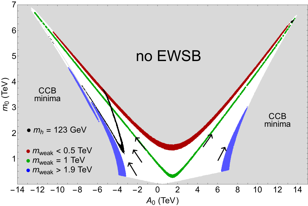
Figure 1: Contours of $m_{weak}$ in the $A_{0}$ vs. $m_{0}$ plane for $m_{1/2}=1$ TeV, $m_{H_{u}}=1.3m_{0}$, $\tan\beta=10$ and $m_{H_{d}}=1$ TeV. The arrows show the direction of statistical/anthropic pull on soft SUSY breaking terms. Within the black contour is where $m_{h}>123$ GeV. There is also a slight black contour in the upper-right horn as well.

Next, we scan over parameter values

$$m_{0}(1,2) : 0-60\ {\rm TeV}$$ (5)

$$m_{0}(3) : 0.1-10\ {\rm TeV}$$ (6)

$$m_{H_{u}} : m_{0}(3)-2m_{0}(3)$$ (7)

$$m_{H_{d}}(\sim m_{A}) : 0.3-10\ {\rm TeV}$$ (8)

$$m_{1/2} : 0.5-3\ {\rm TeV}$$ (9)

$$-A_{0} : 0-50\ {\rm TeV}$$ (10)

$$\mu_{GUT} : \ fixed$$ (11)

$$\tan\beta : 3-60$$ (12)

The soft terms are all scanned according to $f_{SUSY}\sim m_{soft}^{\pm 1}$ while $\mu$ is fixed at a natural value $\mu=150$ GeV. For $\tan\beta$, we scan uniformly. The goal is to take scan upper limits beyond those imposed by $f_{EWSB}$ so the plot upper bounds do not depend on scan limits. The lower limits for the $n=-1$ case are selected in accord with previous scans for $n=1$ with a draw to large soft terms just for consistency. If we lower the lower bound scan limits, then the $n=-1$ histograms will migrate to what becomes even worse discord with experimental limits.

In Fig. 2, we show putative landscape distributions for various NUHM3 parameters. In frame a), we show the distribution for first/second generation scalar masses $m_{0}(1,2)$. For $n=1$, then we see the probability distributions peaks around $m_{0}(1,2)\sim 20$ TeV but extends as high as $\sim 45$ TeV. Such large first/second generation scalar masses provide the decoupling/quasi-degeneracy soluton to the SUSY flavor and CP problems. In contrast, for $n=-1$ then the distribution is sharply peaked near 0 as expected. In frame b), we show the distribution in third generation scalar soft mass $m_{0}(3)$. Here, the $n=1$ distribution peaks at 5 TeV but runs as high as 10 TeV. The $n=-1$ distribution again peaks at zero, which will lead to very light third generation squarks. The distribution in $m_{1/2}$ shown in frame c) for $n=1$ peaks around $m_{1/2}\sim 1.5$ TeV leading to gaugino masses typically beyond the present LHC limits. For $n=-1$, the distribution peaks at low $m_{1/2}$ leading to gauginos that are typically excluded. And in frame d) we see the distribution in trilinear soft term $-A_{0}$. For $n=1$, the distribution has a double peak structure with most values in the multi-TeV range leading to large stop mixing and consequently cancellations in the $\Sigma_{u}^{u}(\tilde{t}_{1,2})$ and upift of $m_{h}$ to $\sim 125$ GeV. For $n=-1$, then $A_{0}$ peaks around zero, and we expect little stop mixing and lighter values of $m_{h}$.

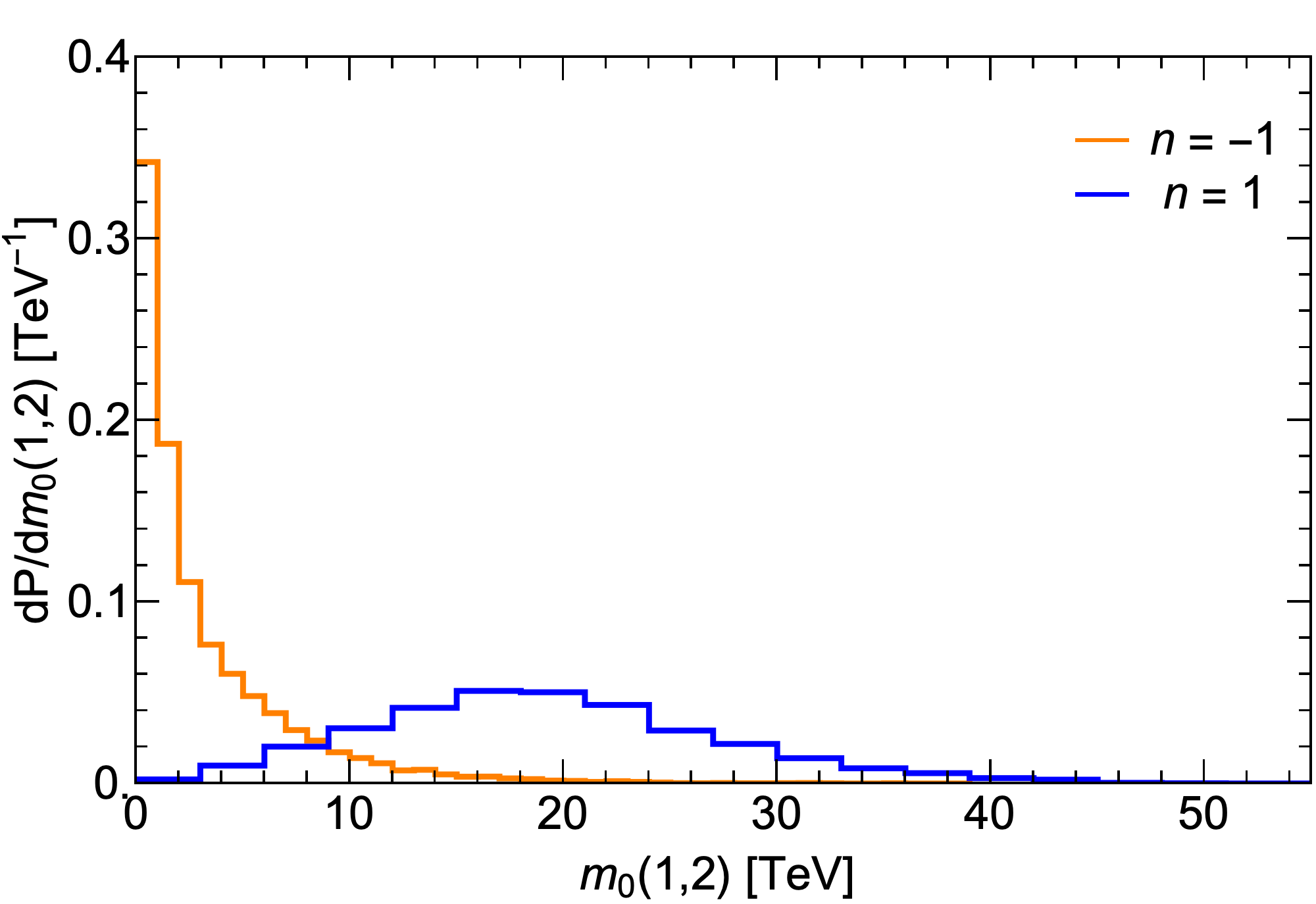
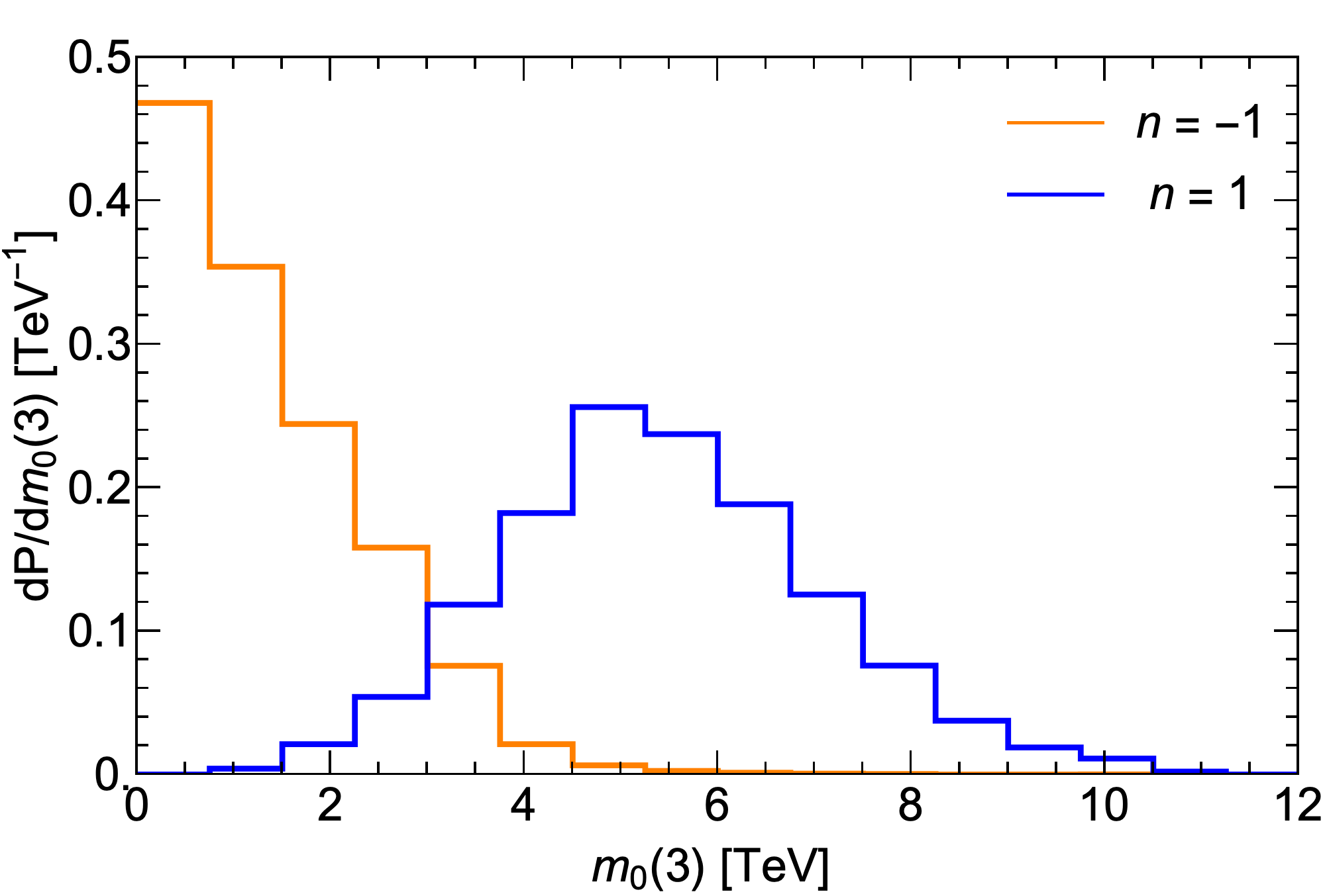
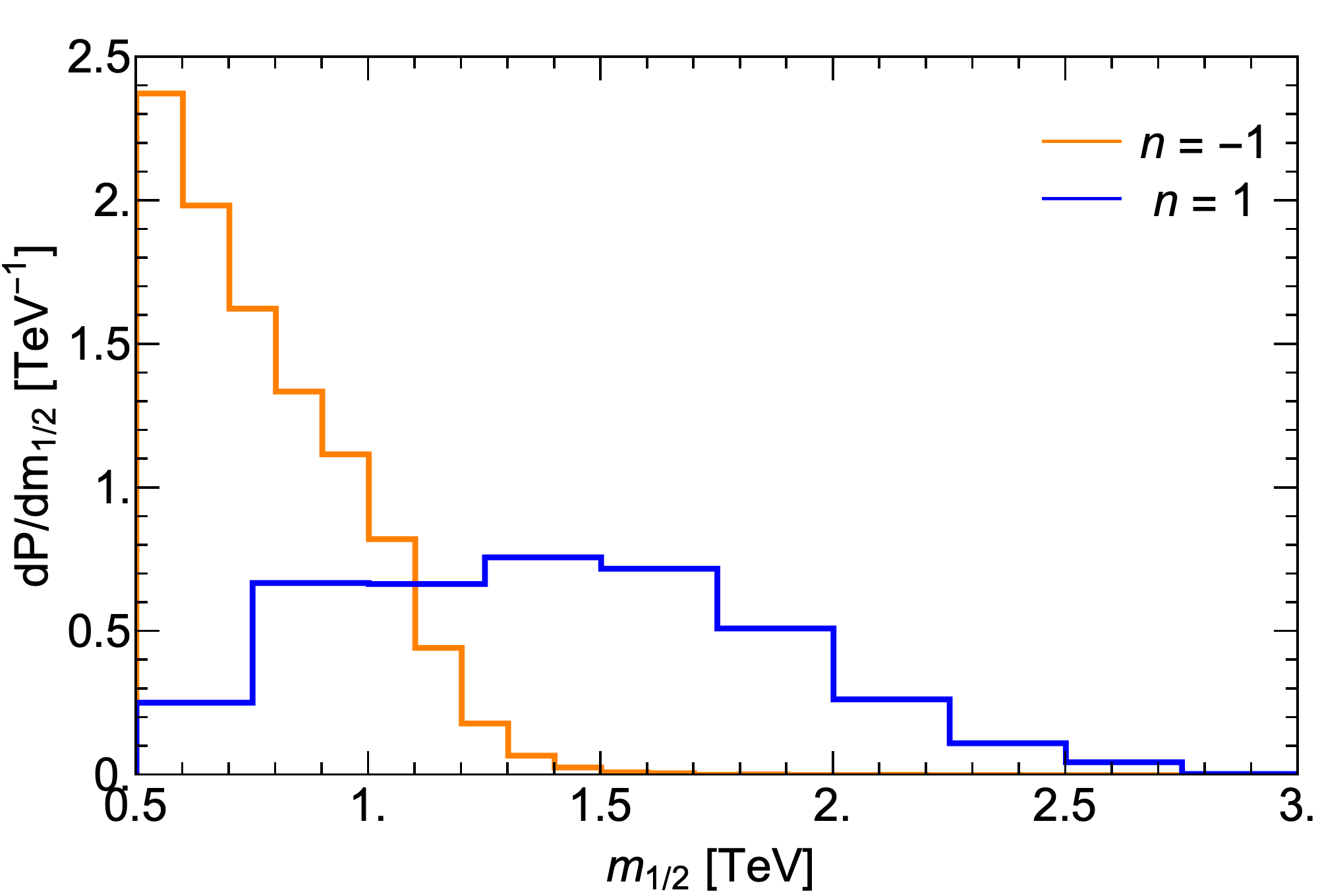
Figure 2: Probability distributions for NUHM3 soft terms a) $m_{0}(1,2)$, b) $m_{0}(3)$, c) $m_{1/2}$ and d) $A_{0}$ from the $f_{SUSY}=m_{soft}^{\pm 1}$ distributions of soft terms in the string landscape with $\mu=150$ GeV.

In Fig. 3, we plot the landscape distributions for light and heavy SUSY Higgs boson masses. In frame a), for $n=1$ we see a distribution with a strong peak around $m_{h}\sim 124-126$ GeV in accord with data. The distribution cuts off for $m_{h}\gtrsim 127$ GeV because otherwise the $\Sigma_{u}^{u}(\tilde{t}_{1,2})$ contributions become too large leading to too large a value of $m_{weak}$ beyond the ABDS window. For $n=-1$, the distribution peaks at $m_{h}\sim 118$ GeV with really no significant probability beyond $m_{h}\sim 124$ GeV. This essentially rules out the $n=-1$ case. In frame b), the distribution in heavy pseudoscalar mass $m_{A}$ is shown. For $n=+1$, the distribution peaks at $m_{A}\sim 2.5$ TeV with a distribution extending as high as $m_{A}\sim 8$ TeV. These values are well beyond recent ATLAS search limits[49] from $H,\ A\rightarrow\tau\bar{\tau}$, which are plotted in the $m_{A}$ vs. $\tan\beta$ plane. For $n=-1$, then we expect rather light $m_{A}$, possibly at a few hundred GeV, leading to large light-heavy Higgs mixing. This also seems in contradiction with LHC results which favor a very SM-like light Higgs as expected in the decoupling limit.

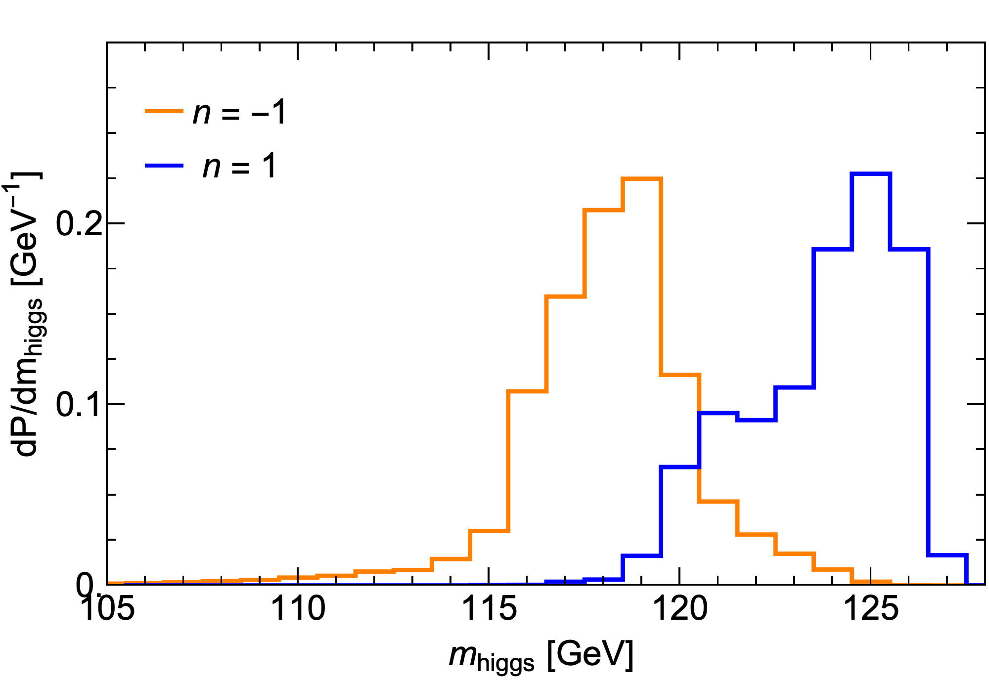
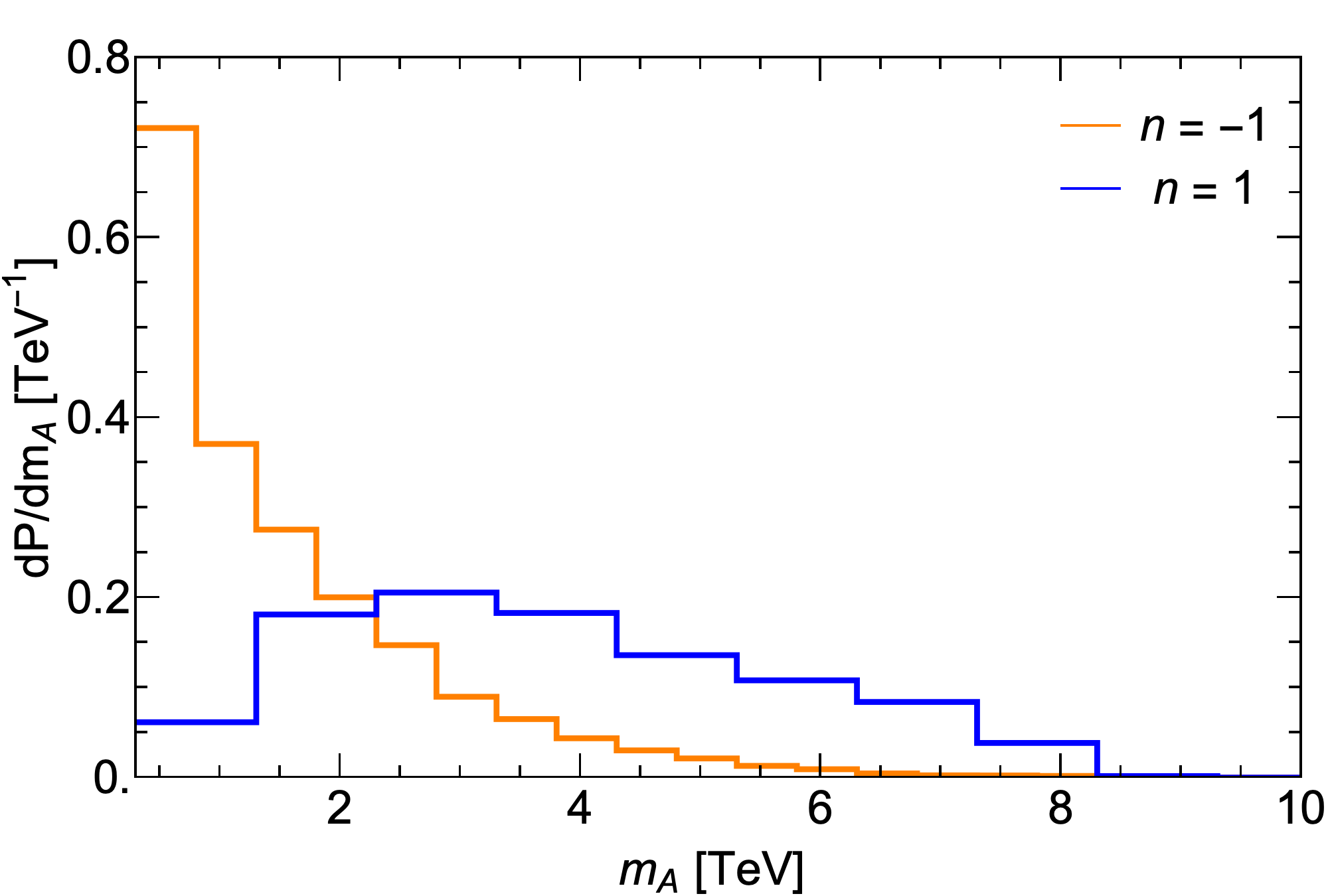
Figure 3: Probability distributions for light Higgs scalar mass a) $m_{h}$ and pseudoscalar Higgs mass b) $m_{A}$ from the $f_{SUSY}=m_{soft}^{\pm 1}$ distributions of soft terms in the string landscape with $\mu=150$ GeV.

In Fig. 4, we plot the expected strongly interacting sparticle mass distributions from the landscape. In frame a), we see for $n=1$ that $m_{\tilde{g}}$ peaks around $m_{\tilde{g}}\sim 2.5-4$ TeV which is well beyond current LHC limits which require $m_{\tilde{g}}\gtrsim 2.1$ TeV. The upper distribution edge extends as far as $m_{\tilde{g}}\sim 6$ TeV. In contrast, for the $n=-1$ distribution, then the bulk of probability is below 2.1 TeV, although a tail does extend somewhat above present LHC bounds. In frame b), we show the distribution in first generation squark mass $m_{\tilde{u}_{L}}$. For $n=1$, the distribution peaks around $m_{\tilde{q}}\sim 20$ TeV but extends to beyond 40 TeV. For $n=-1$, then squarks are typically expected at $m_{\tilde{q}}\lesssim 1-2$ TeV and one would have expected squark discovery at LHC (although a tail extends into the multi-TeV range). In frame c), we show the light top squark mass distribution $m_{\tilde{t}_{1}}$. Here, the $n=1$ distribution lies mainly between $1<m_{\tilde{t}_{1}}<\sim 2.5$ TeV whereas LHC searches require $m_{\tilde{t}_{1}}\gtrsim 1.1$ TeV. For $n=-1$, then somewhat lighter stops are expected although there still is about a 50% probability to lie beyond LHC bounds on $m_{\tilde{t}_{1}}$. In frame d), we show the distribution in $m_{\tilde{t}_{2}}$. For $n=1$, we expect $m_{\tilde{t}_{2}}\sim 2-6$ TeV whilst for $n=-1$ then we expect instead that $m_{\tilde{t}_{2}}\sim 1-3$ TeV.

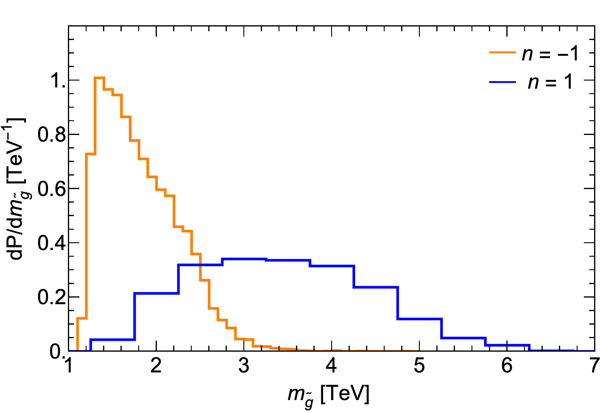
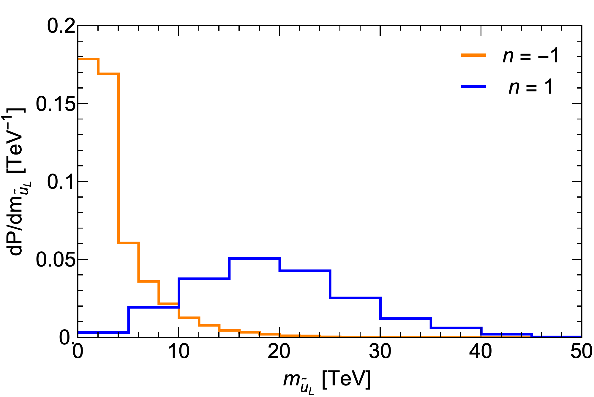
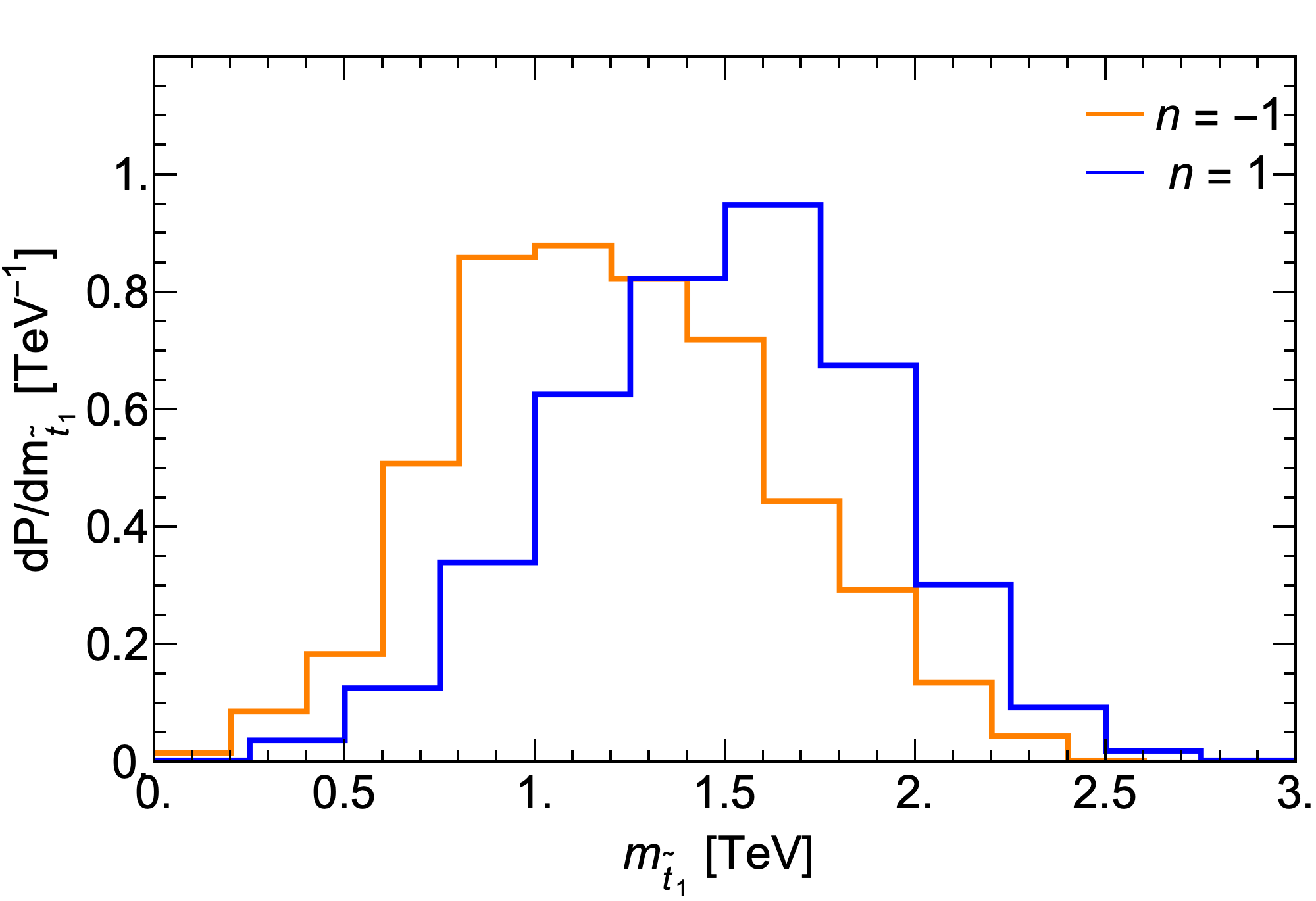
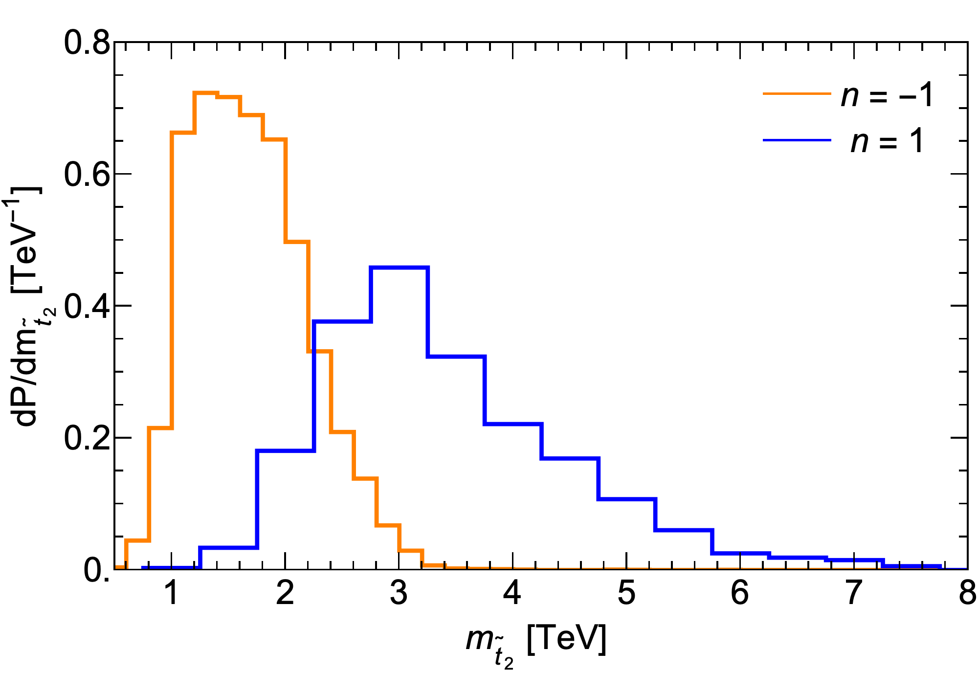
Figure 4: Probability distributions for a) $m_{\tilde{g}}$, b) $m_{\tilde{u}_{L}}$, c) $m_{\tilde{t}_{1}}$ and d) $m_{\tilde{t}_{2}}$ from the $f_{SUSY}=m_{soft}^{\pm 1}$ distributions of soft terms in the string landscape with $\mu=150$ GeV.

3 Stringy naturalness

For the case of the string theory landscape, in Ref. [50] Douglas has introduced the concept of stringy naturalness:

Stringy naturalness: the value of an observable ${\cal O}_{2}$ is more natural than a value ${\cal O}_{1}$ if more phenomenologically viable vacua lead to ${\cal O}_{2}$ than to ${\cal O}_{1}$.

We can compare the usual naturalness measure $\Delta_{BG}$ to what is expected from stringy naturalness in the $m_{0}$ vs. $m_{1/2}$ plane[51]. We generate SUSY soft parameters in accord with Eq. 2 for values of $n=2n_{F}+n_{D}-1=1$ and 4. The more stringy natural regions of parameter space are denoted by the higher density of sampled points.

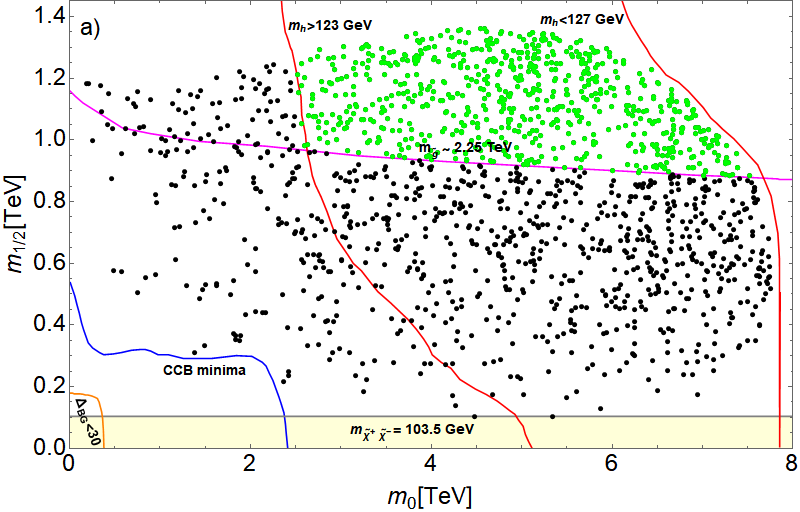
Figure 5: The $m_{0}$ vs. $m_{1/2}$ plane of the NUHM2 model with $A_{0}=-1.6m_{0}$, $\mu=200$ GeV and $m_{A}=2$ TeV and an $n=1$ draw on soft terms, The higher density of points denotes greater stringy naturalness. The LHC Run 2 limit on $m_{\tilde{g}}>2.25$ TeV is shown by the magenta curve. The lower yellow band is excluded by LEP2 chargino pair search limits. The green points are LHC-allowed while black are LHC-excluded.

In Fig. 5, we show the stringy natural regions for the case of $n=1$. Of course, no dots lie below the CCB boundary since such minima must be vetoed as they likely lead to an unlivable pocket universe. Beyond the CCB contour, the solutions are in accord with livable vacua. But now the density of points increases with increasing $m_{0}$ and $m_{1/2}$ (linearly, for $n=1$), showing that the more stringy natural regions lie at the highest $m_{0}$ and $m_{1/2}$ values which are consistent with generating a weak scale within the ABDS bounds. Beyond these bounds, the density of points of course drops to zero since contributions to the weak scale exceed its measured value by at least a factor of 4. There is some fluidity of this latter bound so that values of $\Delta_{EW}\sim 20-40$ might also be entertained. The result that stringy naturalness for $n\geq 1$ favors the largest soft terms (subject to $m_{Z}^{PU}$ not ranging too far from our measured value) stands in stark contrast to conventional naturalness which favors instead the lower values of soft terms. Needless to say, the stringy natural favored region of parameter space is in close accord with LHC results in that LHC find $m_{h}=125$ GeV with no sign yet of sparticles.

In Fig. 6, we show the same plane under an $n=4$ draw on soft terms. In this case, the density of dots is clearly highest (corresponding to most stringy natural) at the largest values of $m_{0}$ and $m_{1/2}$ as opposed to naive expectations where the most natural regions are at low $m_{0}$ and $m_{1/2}$. In this sense, under stringy naturalness, a 3 TeV gluino is more natural than a 300 GeV gluino!

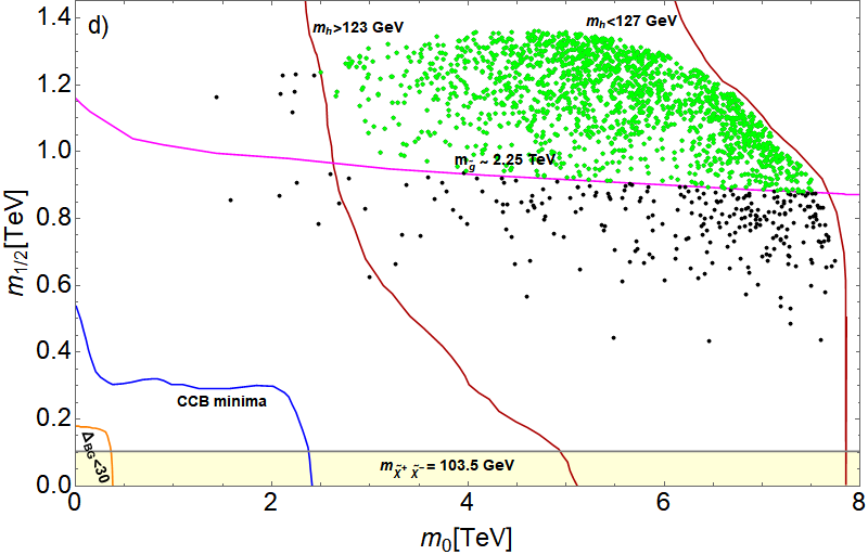
Figure 6: The $m_{0}$ vs. $m_{1/2}$ plane of the NUHM2 model with $A_{0}=-1.6m_{0}$, $\mu=200$ GeV and $m_{A}=2$ TeV and an $n=4$ draw. The higher density of points denotes greater stringy naturalness. The LHC Run 2 limit on $m_{\tilde{g}}>2.25$ TeV is shown by the magenta curve. The lower yellow band is excluded by LEP2 chargino pair search limits. The green points are LHC-allowed while black points are LHC-excluded.

4 Consequences of string landscape for SUSY collider searches

A figurative depiction of the expected sparticle and Higgs mass spectra from the landscape is shown in Fig. 7.

Figure 7: Sparticle and Higgs mass spectra for a natural SUSY benchmark point.

Given such a spectra and the above distributions, we briefly describe expectations for SUSY at future collider options. The big picture is that for a positive power-law draw to large soft terms from the string landscape, then we expect a Higgs mass $m_{h}\sim 125$ GeV with sparticles beyond present LHC search limits: exactly what LHC is seeing so far with $\sqrt{s}=13$ TeV and 139 fb^-1 of integrated luminosity.

4.1 LHC

4.1.1 Light higgsinos

Since the SUSY $\mu$ parameter is SUSY conserving rather than SUSY breaking, it feeds mass to $W,\ Z$ and $h$ and also higgsinos (which mix with gauginos). Gaugino masses are SUSY breaking and we expect the lightest EWinos to be mainly higgsino-like, but not pure higgsino. We expect the higgsino-like lightest EWinos $\tilde{\chi}_{1}^{\pm}$ and $\tilde{\chi}_{1,2}^{0}$ to have mass in the range $\sim 100-350$ GeV. Since the higgsino-like EWinos have very compressed spectra with mass gaps $\sim 5-10$ GeV, then their visible decay products are expected to be very soft and difficult to detect. LHC searches for pair production of higgsino-like EWinos was suggested in Ref. [52] as a probe of low $\mu$ via a soft dimuon trigger. At present, the best search strategy seems to be to look for $pp\rightarrow\tilde{\chi}_{2}^{0}\tilde{\chi}_{1}^{0}+jet$ with $\tilde{\chi}_{2}^{0}\rightarrow\ell^{+}\ell^{-}\tilde{\chi}_{1}^{0}$[53, 54, 55]. For Snowmass 2022, the landscape parameter space has been mapped out in Ref. [56] and improved angular cuts for LHC searches have been proposed in Ref. [57].

4.1.2 Gluino searches

In the landscape, gluinos may range from $\sim 2-6$ TeV while top squarks are in the $1-2.5$ TeV range. This means gluinos should decay to top+stop or else three-body modes to top and bottom quarks[58, 59]. The HL-LHC $5\sigma$ reach assuming 3000 fb^-1 is found to be $m_{\tilde{g}}\sim 2.7$ TeV so there is some possibility these will be discovered at LHC but more likely a higher energy hadron collider with $\sqrt{s}\gtrsim 30$ TeV will be needed[60, 61, 62].

4.1.3 Top squark pair searches

In landscape SUSY, we expect light top squarks with mass $m_{\tilde{t}_{1}}\sim 1-2.5$ TeV whilst the current LHC limits require $m_{\tilde{t}_{1}}>1.1$ TeV. The reach of HL-LHC with 3000 fb^-1 extends to $m_{\tilde{t}_{1}}\sim 1.3-1.7$ TeV. Thus, a higher energy hadron collider will be needed to probe the entire expected light stop mass range[60, 61, 62]. An important feature of landscape SUSY is that top squarks should be nearly maximally mixed due to the required large weak scale value of the trilinear soft term $A_{t}$.

4.1.4 Same-sign diboson signature

A qualitatively new signature for SUSY arises in natural models when $\mu$ is small. The reaction $pp\rightarrow\tilde{\chi}_{2}^{\pm}\tilde{\chi}_{4}^{0}$ whre the EWinos are mainly wino-like can occur at high rates followed by decay to same-sign $W$ bosons. This gives a unique SS dilepton plus MET signature with minimal jet activity (just that from ISR) in distinction to SS dileptons from gluino and squark production where substantial jet activity is expected. Signal and background and LHC reach have been plotted out in Ref’s [63, 64, 65].

4.2 Linear $e^{+}e^{-}$ collider

4.2.1 Direct production of light higgsinos

Since light higgsinos are expeted in landscape SUSY with radiatively-driven naturalness, then it makes sense to build something like the International Linear $e^{+}e^{-}$ Collider (ILC). The ILC is touted as a Higgs factory, but if $\sqrt{s}>2m(higgsino)\sim 250-700$ GeV, then it may turn out to be a higgsino factory as well[66]. The soft dileptons arising from higgsino pair production ($e^{+}e^{-}\rightarrow\tilde{\chi}_{1}^{+}\tilde{\chi}_{1}^{-}$ and $\tilde{\chi}_{1}^{0}\tilde{\chi}_{2}^{0}$) should be easily seen at ILC and their invariant mass and energy spectra will allow precision determination of their masses and mixings. One may even test gaugino mass unification[67].

4.2.2 Precision Higgs measurements at a Higgs factory

A primary goal of an $e^{+}e^{-}$ machine operating with $\sqrt{s}>m_{Z}+m_{h}$ is that it can precisely measure Higgs boson properties, especially coupling strengths $\kappa_{i}$ which could show deviations from SM predictions. In landscape SUSY, since the soft terms are pulled to large values, one gets decoupling and the expected Higgs couplings should look very SM-like[68].

5 Consequences for WIMP and axion searches

In natural SUSY with light higgsinos, the lightest neutralino is higgsino-like and typically thermally underproduced by about a factor $5-15$. If the underdensity of neutralinos is augmented by non-thermal higgsino production in the early universe, then higgsino-only dark matter seems excluded by direct and indirect DM detection experiments[69]. However, since axions are needed to solve the strong CP problem, then a neutralino/axion dark matter mixture is to be expected[70]. In SUSY context with two Higgs doublets, the SUSY DFSZ axion model is naturally expected[71, 72], and axions tend to make up the bulk of the DM abundance. The lower neutralino DM abundance allows light higgsinos to escape DD and IDD DM bounds[73]. The full mixed axion/higgsino DM abundance reqires solution of eight coupled Boltzmann equations which include the effects of axinos, axions, saxions and gravitinos[74, 75]. The axions are more difficult to detect than otherwise projected since now higgsinos circulate in the axion-$\gamma$-$\gamma$ loop and reduce the axion-photon coupling to tiny levels[76].

6 Consequences for $(g-2)_{\mu}$

The $a_{\mu}\equiv(g-2)_{\mu}/2$ anomaly has recently been reinforced by first data from the Fermilab E989 experiment. To match the anomaly, SUSY theories typically need light smuons and mu-sneutrinos. The landscape tends to pull first/second generation sfermions into the 10-40 TeV range so that $a_{\mu}$ should look very SM-like. In this case, we would expect little or no anomaly[77].

7 Conclusions

The emergence of the string landscape of vacua has exciting consequences for SUSY phenomenology (in addition to providing a solution to the CC problem). With of order $10^{500}$ vacua to explore, statistical methods can be brought to bear, and may even place string theory on a long-awaited predictive footing. We present here a mini-review of our work on the topic of stringy naturalness. We examined two main scenarios: a power-law draw on soft terms to large ($n=1$) or small ($n=-1$) soft terms. The former is motivated by the expectation of SUSY breaking by a single $F$ term which is distributed uniformly as a complex number on the landscape, and by KKLT moduli stabilization. The latter is motivated by an expectation that the SUSY breaking scale is distributed uniformly over the decades of possibilities and arises in LVS moduli stabilization. These statistical expectations must be tempered by the anthropic requirement that the derived value for the weak scale in each pocket universe must lie within the ABDS window of values. The LHC data clearly are in accord with the $n\geq 1$ statistics, as they predict $m_{h}\sim 125$ GeV with sparticles typically beyond present LHC search limits. We also discussed these implications for LHC SUSY searches and for WIMP and axion dark matter searches, since we expect dark matter to consist of a WIMP/axion admixture.

Acknowledgements:

This work is a Snowmass 2022 whitepaper. This material is based upon work supported by the U.S. Department of Energy, Office of Science, Office of High Energy Physics under Award Number DE-SC-0009956 and DE-SC-001764. Some of the computing for this project was performed at the OU Supercomputing Center for Education and Research (OSCER) at the University of Oklahoma (OU). The work of DS was supported by the Ministry of Science and Technology (MOST) of Taiwan under Grant No. 110-2811-M-002-574.

References

- [1] M. B. Green, J. H. Schwarz, E. Witten, SUPERSTRING THEORY. VOL. 1: INTRODUCTION, Cambridge Monographs on Mathematical Physics, 1988.
- [2] M. B. Green, J. H. Schwarz, E. Witten, SUPERSTRING THEORY. VOL. 2: LOOP AMPLITUDES, ANOMALIES AND PHENOMENOLOGY, 1988.
- [3] P. Horava, E. Witten, Eleven-dimensional supergravity on a manifold with boundary, Nucl. Phys. B 475 (1996) 94–114. arXiv:hep-th/9603142, doi:10.1016/0550-3213(96)00308-2.
- [4] P. Candelas, G. T. Horowitz, A. Strominger, E. Witten, Vacuum Configurations for Superstrings, Nucl. Phys. B 258 (1985) 46–74. doi:10.1016/0550-3213(85)90602-9.
- [5] J. Conlon, The What and Why of Moduli, Adv. Ser. Direct. High Energy Phys. 22 (2015) 11–22. doi:10.1142/9789814602686_0002.
- [6] R. Bousso, J. Polchinski, Quantization of four form fluxes and dynamical neutralization of the cosmological constant, JHEP 06 (2000) 006. arXiv:hep-th/0004134, doi:10.1088/1126-6708/2000/06/006.
- [7] M. R. Douglas, S. Kachru, Flux compactification, Rev. Mod. Phys. 79 (2007) 733–796. arXiv:hep-th/0610102, doi:10.1103/RevModPhys.79.733.
- [8] S. Ashok, M. R. Douglas, Counting flux vacua, JHEP 01 (2004) 060. arXiv:hep-th/0307049, doi:10.1088/1126-6708/2004/01/060.
- [9] W. Taylor, Y.-N. Wang, The F-theory geometry with most flux vacua, JHEP 12 (2015) 164. arXiv:1511.03209, doi:10.1007/JHEP12(2015)164.
- [10] S. Weinberg, Anthropic Bound on the Cosmological Constant, Phys. Rev. Lett. 59 (1987) 2607. doi:10.1103/PhysRevLett.59.2607.
- [11] A. H. Guth, Inflation and eternal inflation, Phys. Rept. 333 (2000) 555–574. arXiv:astro-ph/0002156, doi:10.1016/S0370-1573(00)00037-5.
- [12] A. Linde, A brief history of the multiverse, Rept. Prog. Phys. 80 (2) (2017) 022001. arXiv:1512.01203, doi:10.1088/1361-6633/aa50e4.
- [13] H. Martel, P. R. Shapiro, S. Weinberg, Likely values of the cosmological constant, Astrophys. J. 492 (1998) 29. arXiv:astro-ph/9701099, doi:10.1086/305016.
- [14] H. Baer, X. Tata, Weak scale supersymmetry: From superfields to scattering events, Cambridge University Press, 2006.
- [15] H. Baer, V. Barger, S. Salam, D. Sengupta, K. Sinha, Status of weak scale supersymmetry after LHC Run 2 and ton-scale noble liquid WIMP searches, Eur. Phys. J. ST 229 (21) (2020) 3085–3141. arXiv:2002.03013, doi:10.1140/epjst/e2020-000020-x.
- [16] K. J. Bae, H. Baer, V. Barger, D. Sengupta, Revisiting the SUSY problem and its solutions in the LHC era, Phys. Rev. D 99 (11) (2019) 115027. arXiv:1902.10748, doi:10.1103/PhysRevD.99.115027.
- [17] H. Baer, V. Barger, P. Huang, D. Mickelson, A. Mustafayev, X. Tata, Radiative natural supersymmetry: Reconciling electroweak fine-tuning and the Higgs boson mass, Phys. Rev. D 87 (11) (2013) 115028. arXiv:1212.2655, doi:10.1103/PhysRevD.87.115028.
- [18] H. Baer, V. Barger, D. Martinez, Comparison of SUSY spectra generators for natural SUSY and string landscape predictions (11 2021). arXiv:2111.03096.
- [19] H. Baer, V. Barger, P. Huang, A. Mustafayev, X. Tata, Radiative natural SUSY with a 125 GeV Higgs boson, Phys. Rev. Lett. 109 (2012) 161802. arXiv:1207.3343, doi:10.1103/PhysRevLett.109.161802.
- [20] H. Baer, V. Barger, S. Salam, D. Sengupta, String landscape guide to soft SUSY breaking terms, Phys. Rev. D 102 (7) (2020) 075012. arXiv:2005.13577, doi:10.1103/PhysRevD.102.075012.
- [21] M. R. Douglas, Statistical analysis of the supersymmetry breaking scale (5 2004). arXiv:hep-th/0405279.
- [22] L. Susskind, Supersymmetry breaking in the anthropic landscape, in: From Fields to Strings: Circumnavigating Theoretical Physics: A Conference in Tribute to Ian Kogan, 2004, pp. 1745–1749. arXiv:hep-th/0405189, doi:10.1142/9789812775344_0040.
- [23] N. Arkani-Hamed, S. Dimopoulos, S. Kachru, Predictive landscapes and new physics at a TeV (1 2005). arXiv:hep-th/0501082.
- [24] F. Denef, M. R. Douglas, Distributions of nonsupersymmetric flux vacua, JHEP 03 (2005) 061. arXiv:hep-th/0411183, doi:10.1088/1126-6708/2005/03/061.
- [25] M. Dine, E. Gorbatov, S. D. Thomas, Low energy supersymmetry from the landscape, JHEP 08 (2008) 098. arXiv:hep-th/0407043, doi:10.1088/1126-6708/2008/08/098.
- [26] M. Dine, The Intermediate scale branch of the landscape, JHEP 01 (2006) 162. arXiv:hep-th/0505202, doi:10.1088/1126-6708/2006/01/162.
- [27] I. Broeckel, M. Cicoli, A. Maharana, K. Singh, K. Sinha, Moduli Stabilisation and the Statistics of SUSY Breaking in the Landscape, JHEP 10 (2020) 015. arXiv:2007.04327, doi:10.1007/JHEP09(2021)019.
- [28] V. Balasubramanian, P. Berglund, J. P. Conlon, F. Quevedo, Systematics of moduli stabilisation in Calabi-Yau flux compactifications, JHEP 03 (2005) 007. arXiv:hep-th/0502058, doi:10.1088/1126-6708/2005/03/007.
- [29] S. Kachru, R. Kallosh, A. D. Linde, S. P. Trivedi, De Sitter vacua in string theory, Phys. Rev. D 68 (2003) 046005. arXiv:hep-th/0301240, doi:10.1103/PhysRevD.68.046005.
- [30] V. Agrawal, S. M. Barr, J. F. Donoghue, D. Seckel, Viable range of the mass scale of the standard model, Phys. Rev. D 57 (1998) 5480–5492. arXiv:hep-ph/9707380, doi:10.1103/PhysRevD.57.5480.
- [31] V. Agrawal, S. M. Barr, J. F. Donoghue, D. Seckel, Anthropic considerations in multiple domain theories and the scale of electroweak symmetry breaking, Phys. Rev. Lett. 80 (1998) 1822–1825. arXiv:hep-ph/9801253, doi:10.1103/PhysRevLett.80.1822.
- [32] H. Baer, V. Barger, D. Martinez, S. Salam, Radiative natural supersymmetry emergent from the string landscape (2 2022). arXiv:2202.07046.
- [33] J. R. Ellis, K. A. Olive, Y. Santoso, The MSSM parameter space with nonuniversal Higgs masses, Phys. Lett. B 539 (2002) 107–118. arXiv:hep-ph/0204192, doi:10.1016/S0370-2693(02)02071-3.
- [34] J. R. Ellis, T. Falk, K. A. Olive, Y. Santoso, Exploration of the MSSM with nonuniversal Higgs masses, Nucl. Phys. B 652 (2003) 259–347. arXiv:hep-ph/0210205, doi:10.1016/S0550-3213(02)01144-6.
- [35] H. Baer, A. Mustafayev, S. Profumo, A. Belyaev, X. Tata, Direct, indirect and collider detection of neutralino dark matter in SUSY models with non-universal Higgs masses, JHEP 07 (2005) 065. arXiv:hep-ph/0504001, doi:10.1088/1126-6708/2005/07/065.
- [36] W. Buchmuller, K. Hamaguchi, O. Lebedev, M. Ratz, Local grand unification, in: GUSTAVOFEST: Symposium in Honor of Gustavo C. Branco: CP Violation and the Flavor Puzzle, 2005, pp. 143–156. arXiv:hep-ph/0512326.
- [37] F. Gabbiani, E. Gabrielli, A. Masiero, L. Silvestrini, A Complete analysis of FCNC and CP constraints in general SUSY extensions of the standard model, Nucl. Phys. B 477 (1996) 321–352. arXiv:hep-ph/9604387, doi:10.1016/0550-3213(96)00390-2.
- [38] H. Baer, V. Barger, M. Padeffke-Kirkland, X. Tata, Naturalness implies intra-generational degeneracy for decoupled squarks and sleptons, Phys. Rev. D 89 (3) (2014) 037701. arXiv:1311.4587, doi:10.1103/PhysRevD.89.037701.
- [39] N. Arkani-Hamed, H. Murayama, Can the supersymmetric flavor problem decouple?, Phys. Rev. D 56 (1997) R6733–R6737. arXiv:hep-ph/9703259, doi:10.1103/PhysRevD.56.R6733.
- [40] H. Baer, C. Balazs, P. Mercadante, X. Tata, Y. Wang, Viable supersymmetric models with an inverted scalar mass hierarchy at the GUT scale, Phys. Rev. D 63 (2001) 015011. arXiv:hep-ph/0008061, doi:10.1103/PhysRevD.63.015011.
- [41] H. Baer, V. Barger, D. Sengupta, Landscape solution to the SUSY flavor and CP problems, Phys. Rev. Res. 1 (3) (2019) 033179. arXiv:1910.00090, doi:10.1103/PhysRevResearch.1.033179.
- [42] H. P. Nilles, P. K. S. Vaudrevange, Geography of Fields in Extra Dimensions: String Theory Lessons for Particle Physics, Mod. Phys. Lett. A 30 (10) (2015) 1530008. arXiv:1403.1597, doi:10.1142/S0217732315300086.
- [43] H. Baer, V. Barger, H. Serce, X. Tata, Natural generalized mirage mediation, Phys. Rev. D 94 (11) (2016) 115017. arXiv:1610.06205, doi:10.1103/PhysRevD.94.115017.
- [44] H. Baer, V. Barger, D. Sengupta, Anomaly mediated SUSY breaking model retrofitted for naturalness, Phys. Rev. D 98 (1) (2018) 015039. arXiv:1801.09730, doi:10.1103/PhysRevD.98.015039.
- [45] H. Baer, V. Barger, D. Sengupta, Mirage mediation from the landscape, Phys. Rev. Res. 2 (1) (2020) 013346. arXiv:1912.01672, doi:10.1103/PhysRevResearch.2.013346.
- [46] H. Baer, V. Barger, M. Savoy, H. Serce, The Higgs mass and natural supersymmetric spectrum from the landscape, Phys. Lett. B 758 (2016) 113–117. arXiv:1602.07697, doi:10.1016/j.physletb.2016.05.010.
- [47] M. Carena, H. E. Haber, Higgs Boson Theory and Phenomenology, Prog. Part. Nucl. Phys. 50 (2003) 63–152. arXiv:hep-ph/0208209, doi:10.1016/S0146-6410(02)00177-1.
- [48] H. Baer, V. Barger, A. Mustafayev, Implications of a 125 GeV Higgs scalar for LHC SUSY and neutralino dark matter searches, Phys. Rev. D 85 (2012) 075010. arXiv:1112.3017, doi:10.1103/PhysRevD.85.075010.
- [49] G. Aad, et al., Search for heavy Higgs bosons decaying into two tau leptons with the ATLAS detector using collisions at TeV, Phys. Rev. Lett. 125 (5) (2020) 051801. arXiv:2002.12223, doi:10.1103/PhysRevLett.125.051801.
- [50] M. R. Douglas, Basic results in vacuum statistics, Comptes Rendus Physique 5 (2004) 965–977. arXiv:hep-th/0409207, doi:10.1016/j.crhy.2004.09.008.
- [51] H. Baer, V. Barger, S. Salam, Naturalness versus stringy naturalness (with implications for collider and dark matter searches), Phys. Rev. Research. 1 (2019) 023001. arXiv:1906.07741, doi:10.1103/PhysRevResearch.1.023001.
- [52] H. Baer, V. Barger, P. Huang, Hidden SUSY at the LHC: the light higgsino-world scenario and the role of a lepton collider, JHEP 11 (2011) 031. arXiv:1107.5581, doi:10.1007/JHEP11(2011)031.
- [53] Z. Han, G. D. Kribs, A. Martin, A. Menon, Hunting quasidegenerate Higgsinos, Phys. Rev. D 89 (7) (2014) 075007. arXiv:1401.1235, doi:10.1103/PhysRevD.89.075007.
- [54] H. Baer, A. Mustafayev, X. Tata, Monojet plus soft dilepton signal from light higgsino pair production at LHC14, Phys. Rev. D 90 (11) (2014) 115007. arXiv:1409.7058, doi:10.1103/PhysRevD.90.115007.
- [55] C. Han, D. Kim, S. Munir, M. Park, Accessing the core of naturalness, nearly degenerate higgsinos, at the LHC, JHEP 04 (2015) 132. arXiv:1502.03734, doi:10.1007/JHEP04(2015)132.
- [56] H. Baer, V. Barger, S. Salam, D. Sengupta, X. Tata, The LHC higgsino discovery plane for present and future SUSY searches, Phys. Lett. B 810 (2020) 135777. arXiv:2007.09252, doi:10.1016/j.physletb.2020.135777.
- [57] H. Baer, V. Barger, D. Sengupta, X. Tata, New angular (and other) cuts to improve the higgsino signal at the LHC (9 2021). arXiv:2109.14030.
- [58] H. Baer, X. Tata, J. Woodside, Phenomenology of Gluino Decays via Loops and Top Quark Yukawa Coupling, Phys. Rev. D 42 (1990) 1568–1576. doi:10.1103/PhysRevD.42.1568.
- [59] H. Baer, C.-h. Chen, M. Drees, F. Paige, X. Tata, Supersymmetry reach of Tevatron upgrades: The Large tan Beta case, Phys. Rev. D 58 (1998) 075008. arXiv:hep-ph/9802441, doi:10.1103/PhysRevD.58.075008.
- [60] H. Baer, V. Barger, J. S. Gainer, P. Huang, M. Savoy, D. Sengupta, X. Tata, Gluino reach and mass extraction at the LHC in radiatively-driven natural SUSY, Eur. Phys. J. C 77 (7) (2017) 499. arXiv:1612.00795, doi:10.1140/epjc/s10052-017-5067-3.
- [61] H. Baer, V. Barger, J. S. Gainer, H. Serce, X. Tata, Reach of the high-energy LHC for gluinos and top squarks in SUSY models with light Higgsinos, Phys. Rev. D 96 (11) (2017) 115008. arXiv:1708.09054, doi:10.1103/PhysRevD.96.115008.
- [62] H. Baer, V. Barger, J. S. Gainer, D. Sengupta, H. Serce, X. Tata, LHC luminosity and energy upgrades confront natural supersymmetry models, Phys. Rev. D 98 (7) (2018) 075010. arXiv:1808.04844, doi:10.1103/PhysRevD.98.075010.
- [63] H. Baer, V. Barger, P. Huang, D. Mickelson, A. Mustafayev, W. Sreethawong, X. Tata, Same sign diboson signature from supersymmetry models with light higgsinos at the LHC, Phys. Rev. Lett. 110 (15) (2013) 151801. arXiv:1302.5816, doi:10.1103/PhysRevLett.110.151801.
- [64] H. Baer, V. Barger, P. Huang, D. Mickelson, A. Mustafayev, W. Sreethawong, X. Tata, Radiatively-driven natural supersymmetry at the LHC, JHEP 12 (2013) 013, [Erratum: JHEP 06, 053 (2015)]. arXiv:1310.4858, doi:10.1007/JHEP12(2013)013.
- [65] H. Baer, V. Barger, J. S. Gainer, M. Savoy, D. Sengupta, X. Tata, Aspects of the same-sign diboson signature from wino pair production with light higgsinos at the high luminosity LHC, Phys. Rev. D 97 (3) (2018) 035012. arXiv:1710.09103, doi:10.1103/PhysRevD.97.035012.
- [66] H. Baer, V. Barger, D. Mickelson, A. Mustafayev, X. Tata, Physics at a Higgsino Factory, JHEP 06 (2014) 172. arXiv:1404.7510, doi:10.1007/JHEP06(2014)172.
- [67] H. Baer, M. Berggren, K. Fujii, J. List, S.-L. Lehtinen, T. Tanabe, J. Yan, ILC as a natural SUSY discovery machine and precision microscope: From light Higgsinos to tests of unification, Phys. Rev. D 101 (9) (2020) 095026. arXiv:1912.06643, doi:10.1103/PhysRevD.101.095026.
- [68] K. J. Bae, H. Baer, N. Nagata, H. Serce, Prospects for Higgs coupling measurements in SUSY with radiatively-driven naturalness, Phys. Rev. D 92 (3) (2015) 035006. arXiv:1505.03541, doi:10.1103/PhysRevD.92.035006.
- [69] H. Baer, V. Barger, D. Sengupta, X. Tata, Is natural higgsino-only dark matter excluded?, Eur. Phys. J. C 78 (10) (2018) 838. arXiv:1803.11210, doi:10.1140/epjc/s10052-018-6306-y.
- [70] H. Baer, A. Lessa, S. Rajagopalan, W. Sreethawong, Mixed axion/neutralino cold dark matter in supersymmetric models, JCAP 06 (2011) 031. arXiv:1103.5413, doi:10.1088/1475-7516/2011/06/031.
- [71] K. J. Bae, H. Baer, E. J. Chun, Mainly axion cold dark matter from natural supersymmetry, Phys. Rev. D 89 (3) (2014) 031701. arXiv:1309.0519, doi:10.1103/PhysRevD.89.031701.
- [72] K. J. Bae, H. Baer, E. J. Chun, Mixed axion/neutralino dark matter in the SUSY DFSZ axion model, JCAP 12 (2013) 028. arXiv:1309.5365, doi:10.1088/1475-7516/2013/12/028.
- [73] H. Baer, V. Barger, H. Serce, SUSY under siege from direct and indirect WIMP detection experiments, Phys. Rev. D 94 (11) (2016) 115019. arXiv:1609.06735, doi:10.1103/PhysRevD.94.115019.
- [74] H. Baer, A. Lessa, W. Sreethawong, Coupled Boltzmann calculation of mixed axion/neutralino cold dark matter production in the early universe, JCAP 01 (2012) 036. arXiv:1110.2491, doi:10.1088/1475-7516/2012/01/036.
- [75] K. J. Bae, H. Baer, A. Lessa, H. Serce, Coupled Boltzmann computation of mixed axion neutralino dark matter in the SUSY DFSZ axion model, JCAP 10 (2014) 082. arXiv:1406.4138, doi:10.1088/1475-7516/2014/10/082.
- [76] K. J. Bae, H. Baer, H. Serce, Prospects for axion detection in natural SUSY with mixed axion-higgsino dark matter: back to invisible?, JCAP 06 (2017) 024. arXiv:1705.01134, doi:10.1088/1475-7516/2017/06/024.
- [77] H. Baer, V. Barger, H. Serce, Anomalous muon magnetic moment, supersymmetry, naturalness, LHC search limits and the landscape, Phys. Lett. B 820 (2021) 136480. arXiv:2104.07597, doi:10.1016/j.physletb.2021.136480.