Accessibility Properties of Abnormal Geodesics in Optimal Control Illustrated by two case studies.

Abstract.

In this article, we use two case studies from geometry and optimal control of chemical network to analyze the relation between abnormal geodesics in time optimal control, accessibility properties and regularity of the time minimal value function.

Bernard Bonnard

Institut de Mathématiques de Bourgogne, UMR 5584, Dijon

INRIA, McTAO Team, Sophia Antipolis, France

Jérémy Rouot^∗

Laboratoire de Mathématiques de Bretagne Atlantique, Brest, France

Boris Wembe

Université Paul Sabatier, IRIT, Toulouse, France

(Communicated by the associate editor name)

Introduction

In this article, one considers the time minimal control problem for a smooth system of the form $\frac{\mathrm{d}q}{\mathrm{d}t}=f(q,u)$, where $q\in M$ is an open subset of $\mathbb{R}^{n}$ and the set of admissible control is the set $\mathcal{U}$ of bounded measurable mapping $u(\cdot)$ valued in a control domain $U$, where $U$ is a two-dimensional manifold of $\mathbb{R}^{2}$ with boundary. According to the Maximum Principle [12], time minimal solutions are extremal curves satisfying the constrained Hamiltonian equation

$$\dot{q}=\frac{\partial H}{\partial p},\quad\dot{p}=-\frac{\partial H}{\partial q},$$ (1)

$$H(q,p,u)=\bm{M}(q,p),$$

where $H(q,p,u)=p\cdot F(q,u)$ is the pseudo (or non maximized) Hamiltonian, while $\bm{M}(q,p)=\max_{v\in U}H(q,p,u)$ is the true (maximized) Hamiltonian. A projection of an extremal curve $z=(q,p)$ on the $q$-space is called a geodesic.

Moreover since $\bm{M}$ is constant along an extremal curve and linear with respect to $p$, the extremal can be either exceptional (abnormal) if $\bm{M}=0$ or non exceptional if $\bm{M}\neq 0$. To refine this classification, an extremal subarc can be either regular if the control belongs to the boundary of $U$ or singular if it belongs to the interior and satisfies the condition $\frac{\partial H}{\partial u}=0$.

Taking $q(0)=q_{0}$ the accessibility set $A(q_{0},t_{f})$ in time $t_{f}$ is the set $\cup_{u(\cdot)\in\mathcal{U}}$ $q(t_{f},x_{0},u)$, where $t\mapsto q(\cdot,q_{0},u)$ denotes the solution of the system, with $q(0)=q_{0}$ and clearly since the time minimal trajectories belongs to the boundary of the accessibility set, the Maximum Principle is a parameterization of this boundary. Since this set can have some pathologies [Kupka(1980), p. 174], the analysis of the extremal dynamics is rather intricate. The same holds for the time minimal value function $T(x_{0},x_{1})=\{\min\ t;\ x_{1}=x(t,x_{0},u),\ u(\cdot)\in\mathcal{U}\}$ even in the geodesically complete case.

This provides our geometric framework and to go further in our analysis we shall consider two case studies, each can be taken as a common thread in our analysis.

The first problem is one founding example of calculus of variations and was set originally in 1931 by Zermelo and presented in details by Carathéodory [16, 7], in particular in the case of linear wind for which we shall refer as the historical case along this paper. The problem is a ship navigating on a river with a current and aiming to reach the opposite shore.

Introducing the coordinates $(x,y)$ on the Euclidean space, where the current is given by $\mu(y)\frac{\partial}{\partial x}$ assuming only dependent upon the distance $y$ to the shore and the set of admissible direction is

$$\dot{q}\in F_{0}(q)+U,\quad U=S^{1}.$$

This leads to study the time minimal control problem for the system

$$\dot{\tilde{q}}=F_{0}({\tilde{q}})+\sum_{i=1}^{2}u_{i}\,F_{i}({\tilde{q}}),$$

where $F_{1},F_{2}$ is an orthonormal frame for the Euclidean metric denoted $g=\mathrm{d}x^{2}+\mathrm{d}y^{2}$. From a pure geometric point of view, one can generalize to a Zermelo navigation problem on a surface of revolution $M\subset\mathbb{R}^{3}$, endowed with the induced Riemannian metric, with parallel current and represented as a triplet $(M,F_{0},g)$. The geodesics can be analyzed up to the action of the pseudo-group $G$ of smooth local change of coordinates.

The domain of navigation can be split into two subdomains :

• strong current domain $\|F_{0}\|_{g}>1$

• weak current domain : $\|F_{0}\|_{g}<1$

separated by the transitional case called moderate, with $\|F_{0}\|_{g}=1$. In the historical problem with linear current $F_{0}=y\frac{\partial}{\partial x}$ it is given by $|y|=1$.

Introducing the pseudo-Hamiltonian, one gets

$$H(q,p,u)=H_{0}(q,p)+\sum_{i=1}^{2}u_{i}H_{i}(q,p),$$ (2)

where $H_{i}(z)=p\cdot F_{i}(q),\ i=1,2$ are the Hamiltonian lifts. In the historical problem we introduce the heading angle of the ship $\alpha$ and is the parameterization of the control since $F_{1},F_{2}$ form a frame, extremals are regular since $|u|=1$ belongs to the boundary of $U$: $|u|\leq 1$ and the Maximum Principle leads to compute the true Hamiltonian :

$$H(z)=H_{0}(z)+\sqrt{H_{1}^{2}(z)+H_{2}^{2}(z)}.$$

But an equivalent point of view already introduced in the historical example is to take as accessory control $v=\dot{\alpha}$, derivative of the heading angle.

Such transformation in relation with Goh transformation in optimal control will be called the Carathéodory-Zermelo-Goh transformation. Our study boils down to time minimal control for the single-input control system

$$\dot{\tilde{q}}=X(\tilde{q})+v\,Y(\tilde{q}),\quad v\in\mathbb{R},$$

$X=F_{0}(q)+\cos\alpha F_{1}(q)+\sin\alpha F_{2}(q)$ and $Y=\frac{\partial}{\partial\alpha}$, $\tilde{q}=(q,\alpha)$. Using this rewriting, the maximization condition gives us : $\frac{\partial H}{\partial\alpha}=0$ and hence extremals become singular. Moreover $p=(p_{x},p_{y})$ can be lifted into $\tilde{p}=(p,p_{\alpha})$ and the Maximum Principle leads to the constraints:

$$\tilde{p}(t)\cdot Y(\tilde{q}(t))=\tilde{p}(t)\cdot[Y,X](\tilde{q}(t))=0,$$

where $[Y,X](q)=\frac{\partial Y}{\partial q}(q)X(q)-\frac{\partial X}{\partial q}(q)Y(q)$ is the Lie bracket.

Abnormal geodesics are such that $H(q,p,u)=0$ and they were called limit curves in the historical example. Their geometric interpretation is clear: they exist only in the strong current domain and they are the limit curves of the cone of admissible directions.

One first objective of this article is to make a complete analysis of such abnormal geodesics for the $2d$-Zermelo navigation problem, relating accessibility optimality to regularity of the value function. It completes the series of results presented in [4] describing the relations between singular trajectories in optimal control and feedback invariants. They can be applied to more general problems, where the control is valued in a $2$-dimensional manifold with smooth boundary.

The main point is to analyze in this context optimality properties of geodesics which are non immersed curves using the techniques from singularity theory : computing semi-normal forms and invariants in optimal control, see [11] as a general reference for similar study for singularities of mappings, which goes back to the earliest work of Whitney [15].

The second case of interest consists the control of chemical reactions networks like the McKeithan network: , whose aim is to maximize the production of one species, e.g. $A$. Assuming that the kinetics with respect to the temperature is described by the Arrhenius law the dynamics can be modelled using the graph of reactions. Taking the first derivative of the temperature as the control, which again consists of a Goh transformation, the problem can be transformed into a time minimal control for a single-input affine control system. The optimization problem can be transformed into a time minimal control problem, where the terminal manifold $N$ is given by fixing at the final time a desired concentration of a chosen species, since both problems share the same geodesics. A lot of preliminary work, see [6], was done to analyze this problem. In this article we shall concentrate to the so-called abnormal (exceptional) case where the geodesics are tangent to the terminal manifold $N$. We complete the results from [3] to analyze this case. Note that this problem can be set in the same frame than the Zermelo navigation problem, where a barrier assimilated to a terminal manifold of codimension one is given by $\|F_{0}\|_{g}=1$. Again the geometric frame related to singularity theory was already in the earliest reference: construction of semi-normal form and concept of unfolding in control related to the codimension of the singularities. Recent progress of formal languages are used to describe algorithms to handle complicated computation, in particular in relation with the (reversible) McKeithan network, to complete previous works justified by the network $A\rightarrow B\rightarrow C$.

For both case studies, the abnormal case is related to regularity properties of the value function, and discontinuity of the value function is analyzed in relation with classification of accessibility properties.

This article is organized in three sections. In Section 1, we recall general results for time optimality for single-input affine control systems, see [4] as a general reference. Singular trajectories are introduced in relation with feedback invariants and classified with respect to their optimality status. Section 2 analyzes cusp singularities of abnormal geodesics in Zermelo navigation problem, where the historical example is used to compute a semi-normal form. In the final section, we study time minimal syntheses for $3d$-single input system, with terminal manifold of codimension $1$, in relation with the McKeithan network. Calculations are intricate and are handles using semi-normal forms. We concentrate again on the abnormal case, in relation with continuity properties of the value function.

1. General concepts and results from optimal control for single-input control system

We consider a smooth single-input control system of the form

$$\frac{\mathrm{d}q(t)}{\mathrm{d}t}=X(q(t))+u(t)\,Y(q(t)),\ q\in\mathbb{R}^{n},$$

where the control domain $U$ is either $\mathbb{R}$ or the interval $[-1,1]$ and the set of admissible control is the set of measurable mapping on $J=[0,t_{f}(u)]$ valued in $U$ and we denote by $q(\cdot,q_{0},u)$ (in short $q(\cdot)$) defined on a subinterval of $J$ with $q(0)=q_{0}$.

1.1. Maximum Principle

Consider the problem of optimizing the transfer form $q_{0}$ to a smooth submanifold $N$ of $\mathbb{R}^{n}$. Then the Maximum Principle tells us that if a pair $(u(\cdot),q(\cdot))$ is optimal on $[0,t_{f}]$, then there exists an absolutely continuous vector function $p(\cdot)\in\mathbb{R}^{n}\setminus\{0\}$ such that if $H(q,p,u)=p\cdot(X(q)+uY(q))$ denotes the Hamiltonian lift, the following conditions are satisfied

1. The triplet $(q,p,u)$ is solution a.e. on $[0,t_{f}]$ of

   $$\dot{q}=\frac{\partial H}{\partial p},\quad\dot{p}=-\frac{\partial H}{\partial q},$$ (3)

   $$H(q,p,u)=\max_{v\in U}H(q,p,v).$$

2. $\bm{M}(q,p)=\max_{v\in U}H(q,p,v)$ is constant and equal to $-p^{0}$, where $p^{0}$ is non positive.

3. The vector function $p(\cdot)$ satisfies at the final time the transversality condition:

   $$p(t_{f})\perp T_{q(t_{f})}N$$ (4)

Definition 1.1.

A triplet $(q,p,u)$ solution of (3) is called an extremal and the $q$-projection is called a geodesic. If moreover it satisfies the transversality condition (4) it is called a BC-extremal. An extremal is called singular if $H_{Y}(q(t),p(t))=p(t)\cdot Y(q(t))=0$ a.e. on $[0,t_{f}]$. Assume $U=[-1,+1]$, a singular control is called strictly feasible if $u(\cdot)\in]-1,+1[$, saturating at time $t_{s}$ if $|u(t_{s})|=1$. An extremal control is called regular if it is given by $u(t)=\text{sign}(H_{Y}(q(t),p(t)))$ a.e. It is called bang-bang if the number of switches is finite. An extremal is called abnormal (or exceptional) if $p^{0}=0$, so that from the Maximum Principle it is candidate to minimize or maximize the transfer time.

1.2. Computation of the singular controls

If $Z_{1},Z_{2}$ denote two (smooth) vector fields, the Lie bracket is computed with the convention: $[Z_{1},Z_{2}](q)=\frac{\partial Z_{1}}{\partial q}(q)Z_{2}(q)$ $-\frac{\partial Z_{2}}{\partial q}(q)Z_{1}(q)$ and if $H_{1},H_{2}$ are the Hamiltonian lifts of $Z_{1},Z_{2}$, it is related to the Poisson bracket $\{H_{1},H_{2}\}=\mathrm{d}H_{1}(\vec{H}_{2})$ by $\{H_{1},H_{2}\}(q,p)=p\cdot[Z_{1},Z_{2}](q)$. In the singular case, deriving twice with respect to time the equation $H_{Y}(z(t))=0$, where $z(t)=(q(t),p(t))$, one gets:

$$H_{Y}(z(t))=\{H_{Y},H_{X}\}(z(t))=0,$$ (5)

$$\{\{H_{Y},H_{X}\},H_{X}\}(z(t))+u(t)\,\{\{H_{Y},H_{X}\},H_{Y}\}(z(t))=0.$$

Hence, if $\{\{H_{Y},H_{X}\},H_{Y}\}(z(t))$ is not identically zero the singular extremals are given by the constrained Hamiltonian equation:

$$\dot{z}(t)=H_{X}(z(t))+u_{s}(t)\,H_{Y}(z(t)),\text{ with }u_{s}(t)=-\frac{\{\{H_{Y},H_{X}\},H_{X}\}(z(t))}{\{\{H_{Y},H_{X}\},H_{Y}\}(z(t))}$$ (6)

restricted to $H_{Y}=H_{[Y,X]}=0$.

1.3. Action of the feedback pseudo-group $G_{F}$ [8]

Take a pair $(X,Y)$. The set of triplets $\{(\varphi,\alpha,\beta)\}$, where $\varphi$ is a local diffeomorphism and $u=\alpha(x)+\beta(x)v$ with $\beta\neq 0$ is a feedback, acts on the set of pairs $(X,Y)$ and this action defines the pseudo-feedback group $G_{F}$. Each local diffeomorphism $\varphi$ can be lifted into a symplectomorphism using a Matthieu transformation and define an action of the feedback group on (5) using the symplectomorphism only, one has see [4].

Theorem 1.2.

The mapping $\lambda$ which yields for any pair $(X,Y)$ the constrained differential equation (5) is covariant i.e. the following diagram is commutative:

where (5’) consists of the equation (5) with the substitution $(X,Y)\leftarrow(X^{\prime},Y^{\prime})$.

1.4. The $3d$-case

Assume $n=3$. Introduce the following determinants :

$$D=\det(Y,[Y,X],\left[\left[Y,X\right],Y\right]),$$

$$D^{\prime}=\det(Y,[Y,X],\left[\left[Y,X\right],X\right]),$$

$$D^{\prime\prime}=\det(Y,[Y,X],X).$$

Using $H_{Y}=H_{[Y,X]}=H_{[[Y,X],X]}+u_{s}H_{[[Y,X],Y]}=0$, the singular control can be computed eliminating $p$ and depends on $q$ only and this leads to the following:

Proposition 1.

1. Assume $D$ nonzero, the singular controls are defined by the feedback $u_{s}(q)=-D^{\prime}(q)/D(q)$ so that the corresponding geodesics are solutions of the vector field: $X_{s}(q)=X(q)+u_{s}(q)Y(q)$. Abnormal (exceptional) singular geodesics are contained in the determinantal set $D^{\prime\prime}(q)=0$.

2. The map $\lambda:(X,Y)\mapsto X_{s}$ is a covariant, restricting the action of the feedback pseudo-group to change of coordinates only.

1.5. High-order Maximum Principle in the singular case

From [9], in the singular case the generalized Legendre-Clebsch condition

$$\frac{\partial}{\partial u}\frac{\mathrm{d}}{\mathrm{d}t}\frac{\partial H}{\partial u}(q(t))=\left\{\left\{H_{Y},H_{X}\right\},H_{Y}\right\}(q(t))\geq 0$$

is a necessary optimality condition. This leads to the following.

Proposition 2.

In the $3$d-case, candidates to time minimizing are contained in $DD^{\prime\prime}\geq 0$ and candidates to time maximizing are contained in the set $DD^{\prime\prime}\leq 0$. If the corresponding inequalities are strict, they are respectively called hyperbolic or elliptic.

2. Abnormal geodesics in planar Zermelo navigation problems

2.1. Notations and concepts

Let $(M,g,F_{0})$ be a smooth navigation problem, where $(M,g)$ is a Riemannian metric and $F_{0}$ is a vector field defining the current. Our study is local and taking an orthonormal frame $(F_{1},F_{2})$ for the metric $g$, the problem can be written as a time minimal problem for the system

$$\frac{\mathrm{d}q(t)}{\mathrm{d}t}=F_{0}(q(t))+\sum_{i=1,2}u_{i}(t)\,F_{i}(q(t)),\quad q=(x,y),$$ (7)

where the control $u=(u_{1},u_{2})$ is such that $\|u\|\leq 1$. The domain $M$ can be split into domain of strong current with $\|F_{0}\|_{g}>1$ and weak current with $\|F_{0}\|_{g}<1$ and the case transition is called moderate with $\|F_{0}\|_{g}=1$. Let $q_{0}$ be a point in the strong current domain. Then the tangent model at $q_{0}$ is the cone of admissible directions $F_{0}(q_{0})+\sum_{i=1}^{2}u_{i}F_{i}(q_{0})$, $|u_{i}|\leq 1$ whose boundary is limited by two directions called limit curves by Carathéodory. They are precisely the two abnormal directions given by $H(q,p,u)=H_{0}(q,p)+\sum_{i=1}^{2}u_{i}H_{i}(q,p)=0$, where $p$ is the adjoint vector and $H_{i}(q,p)=p\cdot F_{i}(q)$, $i=0,1,2$.

The pseudo-group of local diffeomorphisms on the plane acts on the pair $(F_{0},g)$. The metric can be set locally either in the isothermal form: $g=a(x,y)\,(\mathrm{d}x^{2}+\mathrm{d}y^{2})$ or the polar form $\mathrm{d}r^{2}+m(r,\theta)^{2}\,\mathrm{d}\theta^{2}$, where the corresponding coordinates are respectively called isothermal or polar coordinates. In the case of revolution the isothermal and polar form becomes respectively $a(x)\,(\mathrm{d}x^{2}+\mathrm{d}y^{2})$ and $\mathrm{d}r^{2}+m(r)^{2}\mathrm{d}\theta^{2}$.

In the historical example, the metric is the Euclidean metric $g=\mathrm{d}x^{2}+\mathrm{d}y^{2}$, while the current is given by $F_{0}(q)=y\frac{\partial}{\partial x}$ and taking the line to the shore as parallel, it is oriented along the parallel.

2.2. Maximum Principle

As explained in the introduction the geodesics curves can be parameterized in two different ways using the Maximum Principle.

2.2.1. Direct parameterization

Maximizing the pseudo-Hamiltonian $H(q,u)$ using the constraints $|u|\leq 1$ leads to the following:

Proposition 3.

Denoting $z=(q,p)$ one has:

1. The extremal controls are given by $u_{i}=\frac{H_{i}(z)}{\sqrt{H_{1}(z)^{2}+H_{2}(z)^{2}}}$, $i=1,2$ so that $u_{1}^{2}+u_{2}^{2}=1$.

2. The maximized Hamiltonian is given by $\bm{M}(z)=H_{0}+\sqrt{H_{1}(z)^{2}+H_{2}(z)^{2}}$.

3. The maximized Hamiltonian $\bm{M}$ is constant and can be normalized to $\{\pm 1,0\}$ and the corresponding geodesics are hyperbolic if $\bm{M}=1$, elliptic if $\bm{M}=-1$ and the abnormal case corresponds to $\bm{M}=0$.

2.2.2. Parameterization using the Carathéodory-Zermelo-Goh transformation

Using the heading angle $\alpha$ of the ship amounts to set $u_{1}=\cos\alpha$ and $u_{2}=\sin\alpha$ so that the pseudo-Hamiltonian takes the form

$$H(z)=H_{0}(z)+\cos\alpha H_{1}(z)+\sin\alpha H_{2}(z).$$

The maximization condition leads to $\frac{\partial H}{\partial u}=0$. Denoting $X(\tilde{q})=F_{0}(q)+\cos\alpha F_{1}(q)+\sin\alpha F_{2}(q)$, $Y(\tilde{q})=\frac{\partial}{\partial\alpha}$, where $\tilde{q}=(q,\alpha)$ denotes the extended state space. Using section 1, one has.

Proposition 4.

Geodesics curves are solutions of the dynamics:

$$\dot{\tilde{q}}=X_{s}(\tilde{q})=X(\tilde{q})+u_{s}Y(\tilde{q})$$ (8)

with $u_{s}(\tilde{q})=-D^{\prime}(\tilde{q})/D(\tilde{q})$.

Next we introduce the following crucial set from the control point of view.

Definition 2.1.

Take $(Z_{1},Z_{2})$ two smooth vector fields in $\mathbb{R}^{n}$. The collinear set is the feedback invariant set $\mathcal{C}=\{q;\ Z_{1}(q)\text{ and }Z_{2}(q)\text{ are collinear.}\}$.

One has clearly.

Proposition 5.

In the Goh extension,

1. the collinear set is defined by: $\{\ \exists\alpha;\ F_{0}(q)=\cos\alpha F_{1}(q)+\sin\alpha F_{2}(q)\},$

2. the geodesics curves solutions of (1) are immersed curves outside the collinear set,

3. only abnormal geodesics can be non immersed curves when meeting the collinear set $\|F_{0}\|_{g}=1$.

Before going further in our analysis let us analyze the case of revolution with parallel current as a generalization of the historical example.

2.2.3. The case of revolution with parallel current

In polar coordinates, one has:

$$F_{0}(q)=\mu(r)\frac{\partial}{\partial\theta},\quad g=\mathrm{d}r^{2}+m(r)^{2}\mathrm{d}\theta^{2}$$

so that

$$F_{1}=\frac{\partial}{\partial r},\quad F_{2}=\frac{1}{m(r)}\frac{\partial}{\partial\theta}.$$

We define:

$$X=\cos\alpha\frac{\partial}{\partial r}+\left(\mu(r)+\frac{\sin\alpha}{m(r)}\right)\frac{\partial}{\partial\theta},$$

$$[Y,X]=\sin\alpha\frac{\partial}{\partial r}-\frac{\cos\alpha}{m(r)}\frac{\partial}{\partial\theta},$$

$$\left[\left[Y,X\right],X\right]=\left(-\mu^{\prime}(r)\sin\alpha+\frac{m^{\prime}(r)}{m(r)^{2}}\right)\frac{\partial}{\partial\theta},$$

$$\left[\left[Y,X\right],Y\right]=\cos\alpha\frac{\partial}{\partial r}+\frac{\sin\alpha}{m(r)}\frac{\partial}{\partial\theta}.$$

Lemma 2.2.

Computing we have:

• $D=\frac{1}{m(r)}$,

• $D^{\prime}=-\mu^{\prime}(r)\sin^{2}\alpha+\frac{m^{\prime}(r)}{m(r)^{2}}\sin\alpha$,

• $D^{\prime\prime}=\mu(r)\sin\alpha+\frac{1}{m(r)}$.

Hence $D$ is non zero.

This yields the following proposition.

Proposition 6.

In the case of revolution, with parallel current one has:

1. The pseudo-Hamiltonian in the $\tilde{q}$-representation takes the form:

   $$H=p_{r}\cos\alpha+p_{\theta}\left(\mu(r)+\frac{\sin\alpha}{m(t)}+p^{0}\right).$$

2. The Clairaut relation is satisfied i.e. $p_{\theta}$ is constant and moreover

   $$p_{\theta}\left(\mu(r)+\frac{1}{m(r)\sin\alpha}\right)+p^{0}=0.$$ (9)

3. The geodesics equations $\dot{\tilde{q}}=X(\tilde{q})-\frac{D^{\prime}(\tilde{q})}{D(\tilde{q})}Y(\tilde{q})$ can be integrated by quadratures, solving the implicit equation (9) to integrate the dynamics of the heading angle $\alpha$.

4. Singular points for the geodesics dynamics occur only restricting to abnormal geodesics in $D^{\prime\prime}=0$ when $D^{\prime}=0$.

In the historical example a cusp singularity was observed in [7] and it will serve as a model to analyze the general case in the frame of singularity theory, since integrability is not a technical requirement. One needs to recall some elementary facts.

2.3. A brief recap about cusp singularity theory for geodesics [13]

In our problem, one considers a geodesic curve $t\mapsto\sigma(t)$ defined on $J$ and meeting $\|F_{0}\|_{g}=1$ at $t=t_{0}$. Making a time translation, one can take $J=[-t_{0},t_{0}]$ so that $\sigma$ touches the boundary at $t=0$, so that $\dot{\sigma}(0)=0$.

Definition 2.3.

The point $\sigma(0)$ is a cusp point of order $(p,q)$, $2\leq p\leq q$ if $\sigma^{(p)}(0)$ and $\sigma^{(q)}(0)$ are independent. The point $\sigma(0)$ is called an ordinary cusp (or a semicubical point) if $p=2$, $q=3$, and a ramphoid cusp if $p=2$, $q=4$.

2.3.1. Semicubical point

From [14, p. 56], an algebraic model in $\mathbb{R}[x,y]$ at $\sigma(0)=0$ is given by the equation $x^{3}-y^{2}=0$. Moreover it is the transition between a $\mathbb{R}$-node solution of the equation $x^{3}-x^{2}+y^{2}=0$, where the origin is a double point with two distinct tangents at $0$: $x\pm y=0$ and a $\mathbb{C}-$node solution of $x^{3}+x^{2}+y^{2}=0$ with two complex tangents at $0$ given by $x\pm iy=0$ and with two distinct components $x=y=0$ and a smooth real branch.

A neat description from singularity theory suitable in our analysis is given by [1, p. 65] and is associated to a typical perestroika of a plane curve depending on a parameter and having a semicubical cusp point for some value of the parameters:

Figure 1. Unfolding semicubical cusp.

where the curves sweep an umbrella while their inflectional tangents sweep another umbrella surface.

2.3.2. Semicubical unfolding in the historical example

In the historical example the geodesics equation is given by

$$\frac{\mathrm{d}x}{\mathrm{d}t}=y+\cos\alpha,\quad\frac{\mathrm{d}y}{\mathrm{d}t}=\sin\alpha,\quad\frac{\mathrm{d}\alpha}{\mathrm{d}t}=-1+\alpha^{2}.$$ (10)

The boundary of moderate current is taken as $y=-1$ and making the translation $Y=y+1$and expanding at $\alpha=0$ up to order $2$, the system takes the form

$$\frac{\mathrm{d}x}{\mathrm{d}t}=Y-\alpha^{2}/2,\quad\frac{\mathrm{d}Y}{\mathrm{d}t}=\alpha,\quad\frac{\mathrm{d}\alpha}{\mathrm{d}t}=-1+\alpha^{2}.$$ (11)

and take a point $q_{0}=(x_{0},y_{0},z_{0})$ in a neighbourhood of $0$ in the strong current domain $Y<0$ and let $t\mapsto\sigma(t)$ be a geodesic curve with $\sigma(0)=(x_{0},y_{0},z_{0})$.

Then one has:

Proposition 7.

Fixing $q_{0}$ and considering the geodesics passing through $q_{0}$, we have:

1. The abnormal geodesic meets the boundary at a semicubical cusp with vertical tangent.

2. Hyperbolic geodesics are self-intersecting curves corresponding to a $\mathbb{R}$-node.

3. Elliptic geodesics exist only in the strong current domain $Y<0$ and correspond to a $\mathbb{C}$-node.

Hence geodesics curves form an unfolding of the semicubical cusp with one parameter depending upon the initial heading angle $\alpha_{0}$, see Fig.2.

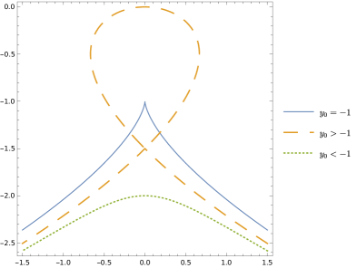
Figure 2. Quickest nautical path as a miniversal unfolding of the generic singularity of the abnormal geodesic.

2.4. The analysis of the geodesics curves near the set $\|F_{0}\|_{g}=1$ and regularity of the time minimal value function.

Proposition 8.

Let $(M,g,F_{0})$ be a two dimensional Zermelo navigation problem and $\tilde{q}_{1}=(q_{1},\alpha_{1})$ be a point in the collinearity set $\mathcal{C}$. Assume that:

• the $q$-projection of $\mathcal{C}$ is a regular curve at $q_{1}$

• the geodesic $\sigma(\cdot)$ is not an immersion at $q_{1}$.

Consider $\tilde{\sigma}:t\mapsto\tilde{\sigma}(t)\coloneqq(\sigma(t),\alpha(t))$, $t\in[t_{1},0],\,t_{1}<0$ to be the geodesic passing through $\tilde{q}_{1}$ at $t=0$ satisfying

$$\dot{\tilde{\sigma}}=X(\tilde{\sigma})-\frac{D^{\prime}(\tilde{\sigma})}{D(\tilde{\sigma})}Y(\tilde{\sigma}),$$ (12)

where $X=F_{0}+\cos\alpha F_{1}+\sin\alpha F_{2}$, $Y=\frac{\partial}{\partial\alpha}$, $D=\det(Y,[Y,X],[[Y,X],Y])$ and $D^{\prime}=\det(Y,[Y,X],[[Y,X],X])$.
Then we have the two cases:

1. $\dot{\alpha}(0)\neq 0$: $\sigma$ has a semicubical cusp at $q_{1}$.

2. $\dot{\alpha}(0)=0$: $\tilde{q}_{1}$ is a singular point with a spectrum $\{0,\pm\lambda\}$ or $\{0,\pm i\,\gamma\}$.

Proof.

Normalization. The problem is local in a neighbourhood of $\tilde{q}_{1}$ and it is enough to show the proposition for $q_{1}=0$. We can choose a coordinate system $(x,y)$ to normalize, at the point $q_{1}$, the vector field $F_{0}$ along the direction $-\frac{\partial}{\partial x}$ i.e. we take two smooth functions $b$ et $c$ such that

$$F_{0}(x,y)=b(x,y)\,\frac{\partial}{\partial x}+c(x,y)\,\frac{\partial}{\partial y},$$

with $b(0,0)=-1$ and $c(0,0)=0$. Then a frame $(F_{1},F_{2})$, orthonormal with respect to the metric $g$ set in the isothermal form $g(x,y)=a(x,y)\,\left(\mathrm{d}x^{2}+\mathrm{d}y^{2}\right)$, can be taken in such way that $F_{0}$ and $F_{1}$ has opposite direction at $q_{1}$:

$$(F_{1},F_{2})=\left(\frac{1}{\sqrt{a(x,y)}}\,\frac{\partial}{\partial x},\frac{1}{\sqrt{a(x,y)}}\,\frac{\partial}{\partial y}\right),$$

where $a$ is a smooth positive function.
In a neighbourhood of $q_{1}$ we write $a(x,y)=\sum_{1\leq i,j\leq k}a_{ij}\,x^{i}y^{j}+\varepsilon_{1}(x,y)$, $b(x,y)=\sum_{1\leq i,j\leq k}b_{ij}\,x^{i}y^{j}+\varepsilon_{2}(x,y)$, $c(x,y)=\sum_{1\leq i,j\leq k}c_{ij}\,x^{i}y^{j}+\varepsilon_{3}(x,y)$, where $\varepsilon_{1},\varepsilon_{2},\varepsilon_{3}$ are terms of order higher than $k$.

The projection of the collinearity set is

$$\{\|F_{0}\|_{g}=1\}=\{a_{00}-1+ (a_{10}-2b_{10})x+(a_{01}-2b_{01})y+\left(c_{01}^{2}-\kappa_{2}\right)\,y^{2}$$

$$+2(c_{01}c_{10}-\kappa_{1})\,xy+\left(c_{10}^{2}-\kappa_{2}^{\prime}\right)\,x^{2}+o(|x,y|^{2})=0\},$$

and is regular near $q_{1}$ and its tangent at $q_{1}$ can be normalized to the horizontal line $y=0$ with $a_{00}=1$, $a_{10}=2b_{10}$ and the constants $\kappa_{1}=-a_{11}/2+3b_{01}b_{10}+b_{11}$ $\kappa_{2}=-a_{02}+3b_{01}^{2}+2b_{02}$, and $\kappa_{2}^{\prime}=-a_{20}+3b_{10}^{2}+2b_{20}$ will have some importance in the sequel. Due to the normalization of $F_{0}$ and $F_{1}$, $\alpha_{1}$ has to be equal to $0$.

Computation. The geodesic $\sigma(\cdot)$ is not an immersion at $q_{1}$ since $\dot{\sigma}(0)=F_{0}(q_{1})+\cos\alpha_{1}F_{1}(q_{1})+\sin\alpha_{1}F_{2}(q_{1})=0$ and denoting by $p(\cdot)$ the corresponding adjoint vector, we have $\bm{M}(q_{1},p(0))=p(0)\cdot\dot{\sigma}(0)=0$ and $\sigma(\cdot)$ is an abnormal geodesic.

Integrating (12), $\tilde{\sigma}(\cdot)$ can be parameterized as

$$\left\{\begin{array}[]{l}\sigma(t)=\left(-\frac{1}{3}t^{3}\delta^{2}+o(t^{3}),\frac{1}{2}t^{2}\delta+o(t^{2})\right)\\ \alpha(t)=t\delta+o(t)\end{array},\right.$$ (13)

where $\delta\coloneqq a_{01}/2-b_{01}$.

The expansions at $\tilde{q}_{1}=0$ of the determinants $D(\tilde{q})$ and $D^{\prime}(\tilde{q})$ are

$$D(\tilde{q}) =1-2b_{01}y-2b_{10}x+o(x,y,\alpha),$$ (14)

$$D^{\prime}(\tilde{q}) =y\left(4a_{01}\delta-3\delta^{2}+\kappa_{2}\right)+x(5b_{10}\delta+\kappa_{1})+c_{01}z-\delta+o(x,y,\alpha).$$

Case $\dot{\alpha}(0)\neq 0$.

In this case $a_{01}/2-b_{01}\neq 0$ and from (13) $\sigma(\cdot)$ has a semicubical cusp at $q_{1}$.

Case $\dot{\alpha}(0)=0$. $\tilde{q}_{1}$ is a singular point of the system $\dot{\tilde{q}}=X_{s}(\tilde{q})$. From (14), for $\delta=0$, $\tilde{\sigma}\equiv 0$ is the integral curve of $X_{s}$ (Lipschitz) with $\tilde{\sigma}(0)=0$, therefore $\tilde{\sigma}$ is reduced to $0$. The characteristic polynomial $\chi$ of the Jacobian matrix $\frac{\partial X_{s}}{\partial\tilde{q}}$ evaluated at $\tilde{q}_{1}$ is

$$\chi(s)=s\,\left(\lambda-s^{2}\right),\quad\lambda=c_{01}^{2}-\kappa_{2},$$

hence the spectrum is $\{0,\pm\sqrt{\lambda}\}$ if $\lambda\geq 0$ or $\{0,\pm i\sqrt{-\lambda}\}$ otherwise. ∎

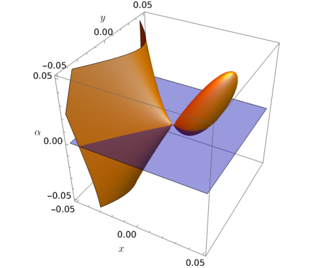
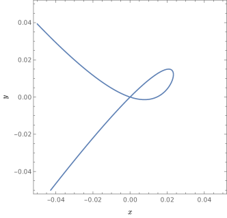
Figure 3. (left) Surface $D^{\prime\prime}(\tilde{q})=0$ for the semi-normal form constructed in the proof of Proposition 8 for $\delta=0$ and random values for the coefficients $a_{ij},b_{ij},c_{ij}$. (right) Intersection of $D^{\prime\prime}=0$ with $\alpha=0$.

Remark 1.

• The spectrum has resonance and in the general case, this leads to moduli in the classification. But since the vector field is geodesic, one has a foliation related to the set $D^{\prime\prime}=0$, while $DD^{\prime\prime}>0$ and $DD^{\prime\prime}<0$ so that we expect a complete classification of the geodesic flow.

• Using the semi-normal form constructed in Proposition 8, the expansion at $\tilde{q}_{1}=0$ of the determinant $D^{\prime\prime}(\tilde{q})$ up to order $2$ is

  $$D^{\prime\prime}(\tilde{q}) =\frac{1}{2}\Big{(}y\left(\delta(4a_{01}y+8b_{10}x-2)-3\delta^{2}y+2\kappa_{1}x+\kappa_{2}y\right)$$

  $$\hskip 128.0374pt+2z(c_{01}y+c_{10}x)+\kappa_{2}^{\prime}x^{2}+z^{2}\Big{)}+o(|x,y,\alpha|^{2}),$$

  and for $\dot{\alpha}=0$ the surface $D^{\prime\prime}(\tilde{q})=0$ is not regular at $\tilde{q}_{1}$ (see Fig. 3).

The following theorem describes the optimality properties of the abnormal and hyperbolic geodesics.

Theorem 2.4.

Let $\tilde{q}_{1}=(q_{1},\alpha_{1})$ such that $q_{1}$ is a semicubical cusp at $t=0$ for the abnormal geodesic $\sigma_{a}(\cdot)$. There exists an neighbourhood $V$ of $q_{1}$, a point $q_{0}$ in $V\cap\sigma_{a}(\cdot)$ in which we have:

1. The abnormal arc is optimal up from $q_{0}$ to the cusp point included.

2. Self-intersecting geodesics starting from $q_{0}$ in a conic neighbourhood of $\alpha_{1}$ are optimal up to the intersection point $q_{1}$ with the abnormal.

3. The value function $T:q_{f}\mapsto T(q_{0},q_{f})$ is discontinuous for each $q_{f}\neq q_{1}$ on the abnormal geodesic $\sigma_{a}(\cdot)$.

Proof.

For $\xi$ in the extented state space, we use the notation $\sigma_{h}(\cdot,\xi)$ (resp. $\sigma_{a}(\cdot,\xi)$) for the projection on the $q$-space of the hyperbolic (resp. exceptional) extremal $\tilde{\sigma}(\cdot,\xi)$ passing through $\xi$ at time $0$. The point $\tilde{q}_{1}$ can be identified to $0$ and we use the same normalization as in the proof of Proposition 8, which leads to consider the semi-normal form

$$F_{0}(x,y)=b(x,y)\,\frac{\partial}{\partial x}+c(x,y)\,\frac{\partial}{\partial y},$$

$$F_{1}=\frac{1}{\sqrt{a(x,y)}}\,\frac{\partial}{\partial x},\quad F_{2}=\frac{1}{\sqrt{a(x,y)}}\,\frac{\partial}{\partial y},$$

with $a(x,y)=\sum_{1\leq i,j\leq k}a_{ij}\,x^{i}y^{j}+\varepsilon_{1}(x,y)$, $b(x,y)=\sum_{1\leq i,j\leq k}b_{ij}\,x^{i}y^{j}+\varepsilon_{2}(x,y)$, $c(x,y)=\sum_{1\leq i,j\leq k}c_{ij}\,x^{i}y^{j}+\varepsilon_{3}(x,y)$ where $\varepsilon_{1},\varepsilon_{2},\varepsilon_{3}$ are terms of order higher than $k$, $a_{00}=1$, $b_{00}=-1$, $c_{00}=0$, $a_{10}=2\,b_{10}$ and $a_{01}-b_{01}\neq 0$.

The proof goes as follows. In relation with Fig.4, we define from $\tilde{q}_{1}$ the points $q_{0}$ and $q_{2}$ on the abnormal geodesics as $\sigma_{a}(t_{0},\tilde{q}_{1})$ and $\sigma_{a}(t_{2},\tilde{q}_{1})$ respectively for some given $t_{0}<t_{2}<0$. In the extended space we take $\tilde{q}_{2}^{\prime}=(q_{2},\alpha_{2}^{\prime})$ and a time $t_{1}<0$ such that $q_{0}$ is reached from $q_{2}$ by a hyperbolic geodesics in time $t_{1}$. The following computation aims to express $\alpha_{2}^{\prime}$ and $t_{1}$ in terms of $t_{0},t_{2}$.

More precisely, for small nonpositive times $t_{0},t_{1},t_{2}$ and small angle $\alpha_{2}^{\prime}$, we expand $q_{2}\coloneqq\sigma_{a}(t_{2},\tilde{q}_{1})$ and $\sigma_{h}(t_{1},\tilde{q}_{2}^{\prime})$ up to order $3$ and we obtain

$$\tilde{\sigma}_{a}(t_{2} ,\tilde{q}_{1})\!=\!\Big{(}-\frac{\delta^{2}}{3}t_{2}^{3},\frac{\delta}{2}t_{2}^{2},\frac{\delta}{12}t_{2}\big{(}-5a_{01}\delta t_{2}^{2}+2c_{01}^{2}t_{2}^{2}-6c_{01}t_{2}+4c_{10}\delta t_{2}^{2}$$

$$\hskip 199.16928pt+2\delta^{2}t_{2}^{2}-2\kappa_{2}t_{2}^{2}+12\big{)}\Big{)}+o(t_{2}^{3}),$$

$$\tilde{\sigma}_{h}(t_{1} ,\tilde{q}_{2}^{\prime})\!=\!\Big{(}\frac{1}{2}\left(2\alpha_{2}^{\prime}t_{1}+\delta t_{1}^{2}+\delta t_{2}^{2}\right),\frac{1}{6}\big{(}-3\alpha_{2}^{\prime 2}t_{1}-\!6\alpha_{2}^{\prime}\delta t_{1}^{2}-2\delta^{2}t_{1}^{3}-\!3\delta^{2}t_{1}t_{2}^{2}-2\delta^{2}t_{2}^{3}\big{)},$$

$$\frac{1}{2}\left(2\alpha_{2}^{\prime}t_{1}+\delta t_{1}^{2}+\delta t_{2}^{2}\right)+\frac{1}{2}c_{01}\delta t_{1}t_{2}^{2},\frac{1}{12}\big{(}3a_{01}\alpha_{2}^{\prime 2}t_{1}-15a_{01}\alpha_{2}^{\prime}\delta t_{1}^{2}-5a_{01}\delta^{2}t_{1}^{3}$$

$$-18a_{01}\delta^{2}t_{1}t_{2}^{2}+12\alpha_{2}^{\prime 2}c_{10}t_{1}-12\alpha_{2}^{\prime 2}\delta t_{1}+6\alpha_{2}^{\prime}c_{01}^{2}t_{1}^{2}+12\alpha_{2}^{\prime}c_{10}\delta t_{1}^{2}+6\alpha_{2}^{\prime}\delta^{2}t_{1}^{2}$$

$$-6\alpha_{2}^{\prime}\kappa_{2}t_{1}^{2}+2c_{01}^{2}\delta t_{1}^{3}+4c_{10}\delta^{2}t_{1}^{3}+2\delta^{3}t_{1}^{3}+18\delta^{3}t_{1}t_{2}^{2}-2\delta\kappa_{2}t_{1}^{3}-6\delta\kappa_{2}t_{1}t_{2}^{2}\big{)}$$

$$-\alpha_{2}^{\prime}c_{01}t_{1}+\alpha_{2}^{\prime}-\frac{1}{2}c_{01}\delta t_{1}^{2}+\delta t_{1}\Big{)}+o(|t_{1},t_{2},\alpha_{2}^{\prime}|^{3}).$$

Computing, the equation

$$q_{0}\coloneqq\sigma_{a}(t_{0},\tilde{q}_{1})=\sigma_{h}(t_{1},\tilde{q}_{2}^{\prime})$$

is satisfied up to order $2$ in $t_{0},t_{1},t_{2},\alpha_{2}^{\prime}$, for

$$t_{1}=t_{2}-t_{0}-2\sqrt{t_{0}^{2}+t_{0}t_{2}+t_{2}^{2}},$$

$$\alpha_{2}^{\prime}=\frac{\delta}{2}\frac{t_{0}^{2}-t_{2}^{2}-t_{1}^{2}}{t_{1}},$$

since $t_{0}<t_{2}$.

Finally, we compare the cost of the abnormal geodesic from $q_{0}$ to $q_{1}$, which is $-t_{0}>0$ and the cost $-t_{1}-t_{2}$ of the concatenation of the hyperbolic geodesic from $q_{0}$ to $q_{2}$ and the abnormal arc from $q_{2}$ to $q_{1}$ as follows:

$$-t_{1}-t_{2} =2\left(\sqrt{(t_{0}-t_{2})^{2}+3t_{2}t_{0}}+t_{0}-t_{2}\right)-t_{0}$$

$$\geq 2\left(|t_{0}-t_{2}|+t_{0}-t_{2}\right)-t_{0}$$

$$\geq-t_{0}.$$

This shows that the value function $q_{f}\mapsto T(q_{0},q_{f})$ is discontinuous if $q_{f}$ is on the abnormal geodesic and $q_{f}\neq q_{1}$. ∎

Figure 4. Hyperbolic and abnormal geodesics in a neighbourhood of the collinearity set.

3. Time minimal exceptional geodesics in optimization of chemical networks

3.1. A brief recap about the optimal control of chemical networks

In this section, we introduce the concepts for the optimization of chemical networks, see [3]. In particular we shall consider the McKeithan network: . The state space is formed by the concentration vector:

$$c=(c_{T},c_{M},c_{A},c_{B})$$

of the respective chemical species. We note $\delta_{1}=c_{T}+c_{A}+c_{B}$, $\delta_{2}=c_{M}+c_{A}+c_{B}$ the first integrals associated to the dynamics and let $x=c_{A}$, $y=c_{B}$, then the system is described by the equation:

$$\dot{x}=-\beta_{2}xv^{\alpha_{2}}-\beta_{3}xv^{\alpha_{3}}-\delta_{3}v\,(x+y)+\delta_{4}v+v\,(x+y)^{2}$$

$$\dot{y}=\beta_{2}xv^{\alpha_{2}}-\beta_{4}yv^{\alpha_{4}}$$

$$\dot{v}=u,\qquad|u|\leq 1,$$

with

$$0\leq x\leq\delta_{1},\ 0\leq y\leq\delta_{2},\ \delta_{3}=\delta_{1}+\delta_{2},\ \delta_{4}=\delta_{1}\delta_{2},$$

the Arrhenius law gives $k_{i}=A_{i}\exp(-E_{i}/RT),\ i=1,2,3,4$ ($E_{i}$ is the activation energy, $T$ is the temperature, $A_{i},R$ are constant) and

$$v=k_{1},\ k_{2}=\beta_{2}v^{\alpha_{2}},\ k_{3}=\beta_{3}v^{\alpha_{3}},k_{4}=\beta_{4}v^{\alpha_{4}}.$$

Maximizing the production of the $A$ species leads to a time minimal control problem with a terminal manifold $N:x=d$, $d$ being the desired production of $A$.

We denote by $\dot{q}=X+u\,Y$, $|u|\leq 1$ the control system.

The singular geodesics are solutions of the dynamics

$$\dot{q}=X+u_{s}\,Y,\quad u_{s}=-D^{\prime}/D.$$

Each optimal solution is a concatenation by arcs $\sigma_{+},\sigma_{-}$, where the control is $u=\pm 1$ and singular arcs $\sigma_{s}$. In this case, the complexity of the surface $D,D^{\prime},D^{\prime\prime}$ contrasts with those of the Zermelo navigation problem given in Lemma 2.2 and we handle here this complexity by the use of different semi-normal forms, constructed for the action of the pseudo–group $\mathcal{G}$ of local diffeomorphisms $\varphi$ such that $\varphi(0)=0$, $\varphi*Y=Y$ and feedback transformation $u\rightarrow-u$ (so that $\sigma_{+}$ and $\sigma_{-}$ can be exchanged).

3.2. General concepts and notation

We consider a local neighborhood $U$ of $q_{0}\in N$. If the optimal control $u^{*}(v)\in[-1,1]$ exists and is unique, it is regular on an open subset of $U$, union of $U_{+}$ where $u^{*}(v)=1$ and $U_{-}$ where $u^{*}(v)=-1$. The surface $S$ which separates $U_{+}$ from $U_{-}$ is subanalytic and can be stratified into

• a switching locus $W$: closure of the set of points where $u^{*}$ is regular and not continuous. We denote by $W_{+}$ (resp. $W_{-}$) the points of $W$ where the optimal control is $+1$ (resp. $-1$) on $N$,

• a cut-locus $C$: closure of the set of points where a trajectory loses its optimality,

• singular locus $\Gamma_{s}$: union of optimal singular trajectories.

and these strata can be approximated by semialgebraic sets using semi-normal forms.

3.3. Local syntheses in the exceptional cases

Take a terminal point $q_{1}$ of $N$, which can be identified to $0$. One wants to describe the time minimal syntheses in a small neighborhood $U$ of $0$. We denote respectively by $\sigma_{\pm}^{0}$, $\sigma_{s}^{0}$ bang and singular arcs terminating at $0$ and we consider only the exceptional case where the arc is tangent to $N$, which splits into the bang exceptional case or the singular exceptional case. The syntheses are described in details in [6, 10] up to the codimension two situations and we recall the main points to be applied to the McKeithan network.

3.3.1. The bang exceptional case

The neighborhood $U$ of $0$ can be split into two domains denoted by $U_{+}$ on which the optimal control is $u=+1$ and the $U_{-}$ where it is given by $u=-1$. We have to consider the two cases.

Generic case (codimension one)

In this case both arcs $\sigma_{+}^{0}$ and $\sigma_{-}^{0}$ arc tangent to $N$ but with a contact of order $2$. Using the concept of unfolding, one can define a $C^{0}$-foliation of $U$ by invariant planes so that in each plane the system takes the semi-normal form:

$$\dot{x}=by+o(|x|,|y|)$$ (15)

$$\dot{y}=X_{2}(x,y)+u,\qquad|u|\leq 1,$$

where $b=n\cdot[Y,X]\neq 0$, which can be normalized to $1$, $n=(1,0)$ being the normal to $N$ identified to $x=0$. Moreover one can assume that $1+X_{2}(0)>0$ and we have two cases.

Proposition 9.

Using the previous normalizations we have two cases described in Fig.3.3.1.

& Case 1: $X_{2}(0)>1$ Case 2: $X_{2}(0)<1$

Figure 5. Local synthesis near $\mathcal{E}$ in the generic case.

The difference between the two cases is related to different accessibility properties of the system. In the case $X_{2}(0)>1$, the target $N$ is not accessible from the points in $x>0$ above the arc $\sigma_{-}^{0}$ terminating at $0$. In the case $X_{2}(0)<1$, each point of $U$ can be steered in minimum time to $N$, the domain $U_{+}$ where the optimal control is $+1$ being $x<0$ and the domain $U_{-}$ with optimal control $-1$ being $x>0$.

Codimension two case

A more complex situation occurs assuming that the arc $\sigma_{-}^{0}$ has a contact of order three with $N$ while $\sigma_{+}^{0}$ has a contact of order two. The optimal syntheses cannot be described by foliating $N$ by $2d$-planes as in the previous cases.

One needs to introduce the following assumptions. We assume that $Y=\frac{\partial}{\partial z}$, $N$ is the plane $x=0$ parameterized as the image of: $(w,s)\mapsto(0,w,s)$. Denoting $n=(1,0,0)$, the normal to $N$ at $0$, we assume

• bang exceptional case: $n\cdot X(0)=0$, $n\cdot[Y,X]\neq 0$,

• $\det(X,Y,[Y,X])\neq 0$ at $0$,

• $\{n\cdot X=0\}\cap N$ is a curve which is neither tangent to $X$ nor to $Y$ at $0$.

We introduce the following normalization: along the $y$-axis, $n\cdot X=0$ and $[X,Y]=\frac{\partial}{\partial x}$.

Using the concept of semi-normal form the optimal syntheses can be described by the following model:

$$\left\{\begin{array}[]{ll}\dot{x}=z\\ \dot{y}=b,&N:(w,s)\mapsto(0,w,s)\\ \dot{z}=1+u+y\end{array},\right.$$ (16)

and we have two types of time minimal syntheses.

Proposition 10.

Assume $b<0$. Then each point of $U$ can be steered to $N$. Moreover

1. $U^{+}\setminus N\subset\{x<0\}$ and $U^{-}\setminus N\subset\{x>0\}$

2. Optimal trajectories $\sigma_{-}$ arrive at any point $(0,w,s<0)$ or $(0,w\geq 0,s)$ of $N\cap U$.

The optimal synthesis is described by Fig.6.

Figure 6. Local synthesis near $\mathcal{E}$ in the codimension $2$ case for $b<0$. The dashed curves are in the region $x\leq<0$.

Proposition 11.

Assume $b>0$. In this case the system is not locally controllable at $0$. We represent on Fig.7 the synthesis in this case.

Figure 7. Local synthesis near $\mathcal{E}$ in the codimension 2 case for $b>0$.

We shall refer to [10] for the full details of the computation and description of the syntheses.

3.3.2. The singular exceptional case

In this case we can assume $Y=\frac{\partial}{\partial z}$, $N$ is the plane $x=0$, the normal to $N$ at $0$ is $n=(1,0,0)$ and moreover:

Singular exceptional case

$$\left\{\begin{array}[]{l}n\cdot X(0)=0\\ n\cdot[Y,X](0)=0\end{array}\right.$$

and we add the following generic conditions

• $X\text{ and }Y\text{ are independent at }0$,

• $\det(Y,[Y,X],\text{ad}^{2}Y\cdot X)\neq 0\text{ at }0$,

• $\{n\cdot X(0)=0\}\cap N\text{ is a curve which is not tangent to }X\text{ at }0$.

Using the concept of semi-normal form the optimal syntheses can be described by the following

$$\left\{\begin{array}[]{l}\dot{x}=y+z^{2}\\ \dot{y}=b+b_{1}\,z\\ \dot{z}=c+u\end{array}.\right.$$ (17)

The different syntheses are described in [10] and we present hereafter a method of computing the time-minimal synthesis for (17) using symbolic computations.

In this model, the exceptional locus $\mathcal{E}\cap N$ is approximated by the parabola: $w+s^{2}=0$ and we denote by $\mathcal{E}_{-}:\{q\in N,\ n\cdot X(q)<0\}$ and $\mathcal{E}_{+}=\{q\in N,\ n\cdot X(q)>0\}$.

We have six cases that we can classify using the model.

• Case 1: $b>0,\ u_{s}(0)>3$.

• Case 2: $b>0,\ 1<u_{s}(0)<3$.

• Case 3: $b>0,\ 0<u_{s}(0)<1$.

• Case 4: $b<0,\ u_{s}(0)>3$.

• Case 5: $b<0,\ 1<u_{s}(0)<3$.

• Case 6: $b<0,\ 0\leq u_{s}(0)<1$.

This describes the complete classification under generic assumptions and the stratification of $S$ can be computed in the original coordinates and applied to the McKeithan network. We illustrate the method in the Case $3$ correcting the results obtained in [10].

Illustration of the method based on symbolic computation.

We present an algorithm to compute an approximation of the surface $S$ in the codimension $2$ case, more specifically we treat the Case 3 described above and given by the model (17) with $b>0$ and such that the singular trajectory arriving at $0$ is not saturating, that is $0\leq b_{1}/2-c<1$.

Method.

The following steps involve symbolic computation to obtain the optimal policy based on [Kupka(1987)].

1.  Take $q(0)=(0,w,s)\in N\cap U$. We first determine the stratification of the surface $N$. Since $Y$ is tangent to $N$, $q(0)$ is a switching point. If $q(0)$ is an ordinary switching point, the optimal control is regular: $u(0)=\text{sign}(p(0)\cdot[Y,X](0))$. If it is a fold point, the optimal control may be singular and the optimal policy is determined using [5]. Note that since $u_{s}(0)=b_{1}/2-c<1$, the singular trajectories are admissible and are either hyperbolic or elliptic, which corresponds respectively to time minimizing or time maximizing trajectories.

2. We then integrate the system backward in time from $q(0)$ and compute the equations characterizing the switching surface, the splitting locus $C_{s}$ and the singular locus $\Gamma_{s}$.

A trajectory $\sigma_{\varepsilon},\varepsilon\in\{-1,1\}$ can switch at time $t_{1}^{\varepsilon}<0$, can intersect the surface $N$ at time $t_{2}^{\varepsilon}<0$ or there may exist a time $t_{3}<0$ and a point $q_{3}\in V$ such that $\exp(-t_{3}(X+Y))(q_{3})=q(0)$, $\exp(-t_{3}(X-Y))(q_{3})\in N$.

The weights of the variable $t,s,w$ is respectively $1,2,1$. We develop the regular flow using Taylor expansion up to order $3$ in $t$, we obtain :

$$\begin{array}[]{llcl}&p_{3}(t_{1}^{\varepsilon})=0&\Rightarrow&t_{1}^{\varepsilon}=\frac{2s}{b_{1}/2-c-\varepsilon}+\dots,\\ &e^{t_{2}^{\varepsilon}(X+\varepsilon Y)}(q(0))\in N&\Rightarrow&t_{2}^{\varepsilon}=\frac{-2}{b}\left(w+s^{2}\right)+\dots,\\ &\exists(t_{3},q)\in\mathbb{R}_{-}^{*}\times U,\ \left\{\begin{array}[]{l}e^{-t_{3}(X+Y)}(q)\in N\\ e^{-t_{3}(X-Y)}(q)\in N\end{array}\right.&\Rightarrow&t_{3}=\frac{3s}{b_{1}/2-c-3}+\dots\end{array}$$ (18)

and a parameterization of

• the switching surface $W_{-}=(x(w,s),y(w,s),z(w,s))$ is

$$x(w,s)=\frac{s^{2}\left(8b_{1}^{2}+\nu_{1}^{2}\right)+3w\nu_{1}^{2}+6bs\nu_{1}}{3\nu_{1}^{3}/4s}+\dots,$$ (19)

$$y(w,s)=\frac{4s\left(b\nu_{1}+b_{1}^{2}s\right)}{\nu_{1}^{2}}+w+\dots,$$

$$z(w,s)=\frac{s(b_{1}+2(c+\varepsilon))}{\nu_{1}}+\dots,$$

where $\nu_{1}=b_{1}-2(c+\varepsilon)$.

• the singular surface $\Gamma_{s}\coloneqq\Gamma_{s}(t,w)$ is

  $$\Gamma_{s}=\left(\frac{bt^{2}}{2}+\frac{b_{1}^{2}t^{3}}{6}+tw,bt+\frac{b_{1}^{2}t^{2}}{4}+w,\frac{b_{1}t}{2}\right)+\dots,$$ (20)

• and the splitting locus $C_{s}=(x(w,s),y(w,s),z(w,s))$ is

$$x(w,s)=\frac{2s^{2}\left(b_{1}c+b_{1}(2b_{1}-9)+2c^{2}+6\right)+w\nu_{2}^{2}}{\nu_{2}^{3}/6s}+\frac{3bs\nu_{2}}{\nu_{2}s/6s}+\dots,$$ (21)

$$y(w,s)=\frac{6s(b\nu_{2}+b_{1}s(b_{1}+c-3))}{\nu_{2}^{2}}+w+\dots,$$

$$z(w,s)=\frac{s(b_{1}+4c)}{\nu_{2}}+\dots.$$

where $\nu_{2}=b_{1}-2c-6$.

3.  The optimal policy is deduced by computing $t^{*}=\max(t_{1}^{\varepsilon},t_{2}^{\varepsilon},t_{3})$ with $\varepsilon=\text{sign}(s\,(n\cdot X(0,w,s)))$ and we represent in Fig.9 the region of $N$ where $t^{*}(w,s)$ corresponds to a switching time, a splitting time or a time at which the trajectory intersects $N$. The surface $S$ separating $U_{+}$ and $U_{-}$ is the union of the switching surface $W_{-}$, the singular surface $\Gamma_{s}$ foliated by singular arcs, the splitting locus $C_{s}$ and a subset $\tilde{\mathcal{E}}_{-}\subset\mathcal{E}_{-}$ from which $\sigma_{\pm}$ intersects $N$ in the green region of Fig. 9. The set $S$ is represented in Fig. 8 together with some trajectories emanating from $N$ to the components of $S$. The green trajectories starting from $\mathcal{E}_{+}$ intersect $N$ in $\tilde{\mathcal{E}}_{-}$.

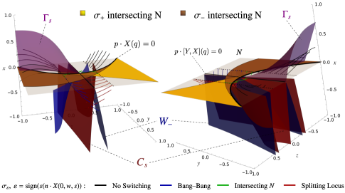
Figure 8. Strata of the surface $S$ separating the regions of $U$ where the control is $\pm 1$ for the model (17) with $b=b_{1}=1,\ c=0$. We also represent the regions where $\sigma_{\pm}$ intersect $N$ for $t<0$ and several trajectories which generate a switching locus and a splitting locus.

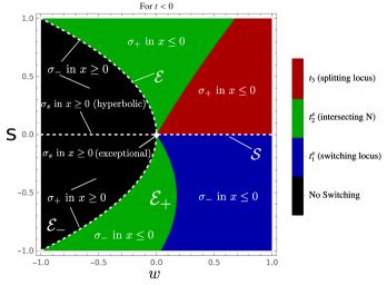
Figure 9. Minimum time $t^{*}=\max(t_{1}^{\varepsilon},t_{2}^{\varepsilon},t_{3})$ to reach $(0,w,s)\in N$ from a neighbourhood $U$ of $0$ for the model (17) with $b=b_{1}=1,\ =c=0$. The exceptional locus is $\mathcal{E}:y=-z^{2}$ and the singular locus is $\mathcal{S}:n\cdot[Y,X](q)=0:z=0$.

Figure 10. Traces of the surfaces $\mathcal{E}$, $\mathcal{C}$ and $\mathcal{S}$ on the terminal manifold $N$ that represent its stratification.

4. Conclusion

In this article, we provide a general framework to analyze accessibility properties of abnormal geodesics using two case studies.

The first case is motivated by the historical Zermelo navigation problem, which is generalized into $2d$-navigation problem. A barrier is formed by decomposing the state space into strong and weak current domains. Abnormal geodesics are limit curves of the set of admissible directions. We show that they reflect on this barrier with a cusp singularity and we analyze this phenomenon using a semi-normal form to evaluate the value function.

The second case is motivated by the problem of optimizing the production of one species for chemical reactors using the derivative of the temperature as control. In this case, the maximized Hamiltonian is nonsmooth and geodesics are concatenation of bang and singular arcs. Again we concentrate to the case of abnormal cases. The various cases are described using semi-normal forms to compute the time minimal synthesis and evaluate the value function.

Received xxxx 20xx; revised xxxx 20xx; early access xxxx 20xx.

References

- [1] Arnol’d, V. I. The theory of singularities and its applications. Lezioni Fermiane. Fermi Lectures, Accademia Nazionale dei Lincei, Rome; Scuola Normale Superiore, Pisa, 1991.
- [2] Arnol’d, V.I. Dynamical systems VI: Singularity Theory I. Encyclopaedia of mathematical sciences Vol. 6, 1993.
- [3] Bakir, T.; Bonnard, B.; Rouot, J. Geometric optimal control techniques to optimize the production of chemical reactors using temperature control. Annu. Rev. Control 48 (2019), 178–192.
- [4] B. Bonnard, M. Chyba, Singular trajectories and their role in control theory. Mathématiques & Applications 40 Springer-Verlag Berlin Heidelberg, 2003 xvi+357.
- [5] Bonnard, B.; Kupka, I. Théorie des singularités de l’application entrée/sortie et optimalité des trajectoires singulières dans le problème du temps minimal. Forum Math. 5, (1993) no.2, pp. 111–159.
- [6] Bonnard, B.; Launay, G.; Pelletier, M. Generic classification of time-minimal syntheses with target of codimension one and applications. Ann. Inst. H. Poincaré Anal. Non Linéaire 14 (1997), no. 1, pp. 55–102.
- [7] Carathéodory, C. Calculus of variations and partial differential equations of the first order. Part I: Partial differential equations of the first order. Inc., San Francisco-London-Amsterdam, 1965 xvi+171 pp.
- [8] Dieudonné, J.A.; Carrell, J.B. Invariant Theory, Old and New. Academic Press, New York, 1971.
- [9] Krener, A.J. The high order maximal principle and its application to singular extremals. SIAM J. Control Optim. 15 (1977), no. 2, pp. 256–293.
- [Kupka(1980)] Kupka, I. Analyse des systèmes. Some problems in accessibility theory. Astérisque, no. 75-76, (1980) pp. 254.
- [Kupka(1987)] Kupka, I. Geometric theory of extremals in optimal control problems. I. The fold and Maxwell case, Trans. Amer. Math. Soc. 299 no.1, (1987) pp. 225–243.
- [10] Launay, G.; Pelletier, M. The generic local structure of time-optimal synthesis with a target of codimension one in dimension greater than two. J. Dynam. Control Systems 3 (1997), no. 2, pp. 165–203.
- [11] Martinet, J. Singularities of smooth functions and maps. London Mathematical Society Lecture Note Series, 58. Cambridge University Press, Cambridge-New York, 1982, xiv+256.
- [12] Pontryagin, L.S.; Boltyanskii, V.G.; Gamkrelidze, R.V.; Mishchenko E.F. The mathematical theory of optimal processes. Oxford, Pergamon Press, 1964.
- [13] Thom, R. Structural stability and morphogenesis. Addison-Wesley Publishing Company, Advanced Book Program, Redwood City, CA (1989).
- [14] Walker, R.J. Algebraic curves. Springer-Verlag, New York, 1978.
- [15] Whitney, H. On singularities of mappings of Euclidean spaces. I. Mappings of the plane into the plane. Ann. of Math., 62 (1955), pp. 374–410.
- [16] Zermelo, E. Über das Navigations problem bei ruhender oder veränderlicher wind-verteilung, Z. Angew. Math. Mech., 11 (1931), no. 2, pp. 114–124.