Nuclear magnetic shielding in HD and HT

Abstract

We perform a calculation of the nuclear magnetic shielding in HD and HT molecules, with complete and perturbative accounts for nuclear masses. From the difference in shielding, we obtain the deuteron and triton magnetic moments in agreement with the CODATA value, with the accuracy limited only by nuclear magnetic resonance measurements. Most importantly, our calculations indicate a potential for improved determination of nuclear magnetic moments.

I Introduction

The most accurate determination of the nuclear magnetic moments is that of the proton, $\mu_{p}=2.792\,847\,344\,62(82)\;\mu_{N}$ [1]. Magnetic moments of all other nuclei have been measured with less or much less accuracy. One of the reasons is the lack of a convenient reference system for which we accurately know the magnetic moment and which can be used for relative measurement of nuclear magnetic resonance (NMR) frequencies. ³He as a noble gas atom would be very convenient once its magnetic moment is accurately measured and the shielding calculated. In fact, the magnetic shielding in the ³He atom has very recently been calculated with the inclusion of leading relativistic and quantum electrodynamics effects to obtain $\sigma=59.967\,029(23)\cdot 10^{-6}$ [2]. Also, the direct measurement of the helion (³He nucleus) magnetic moment, like that of the proton, is being considered by the Heidelberg group [3], which will allow ³He to be set as the ultimate reference system for NMR measurements. In the meantime, we plan to determine the helion magnetic moment from the relative measurements of NMR frequencies between the hydrogen molecule and the ³He atom [4].

Let us now recall the definition of the magnetic shielding. When a molecule is placed in a homogeneous magnetic field $\vec{B}$, its nuclei experience the field that is shielded by the surrounding electrons $(1-{\sigma})\,\vec{B}$. The magnitude of the shielding factor $\sigma$, typically of the order of $10^{-5}$, depends on the particular atomic and molecular system. Ramsey first considered this effect in [5] with the help of the nonrelativistic Hamiltonian with clamped nuclei in the external magnetic field. His result for the isotropic shielding factor $\sigma_{0}$ in the Born-Oppenheimer (BO) approximation is presented in Eq. (23). An immediate conclusion that can be drawn from this formula is that the shielding of the proton and deuteron (triton) in the HD (HT) molecule is the same. Clearly, one has to go beyond the BO approximation and include finite nuclear mass effects in the coupling to the external magnetic field to obtain the difference in the magnetic shielding.

In the past there have been several attempts to calculate this shielding difference in HD (HT). Neronov and Barzakh in 1977 [6] derived the formula for the shielding difference, but they started with the incomplete Hamiltonian, i.e., their formula (4) does not include the nuclear spin-orbit interaction [see $g_{A}-1$ terms in Eq. (LABEL:eq:H) below]. Later, calculations by Jaszuński et al. [7] simulated nonadiabatic effects by an artificial charge difference. Their result of $\delta\sigma({\rm HD})=9\cdot 10^{-9}$, although of the correct magnitude, is not well substantiated from the physical point of view, nor is it complete. In more recent calculations, Golubev and Shchepkin [8] used a more realistic treatment of nonadiabatic effects, but their result of $\delta\sigma({\rm HD})=9\cdot 10^{-9}$ was also incomplete. In Ref. [9] we have derived the complete formula for the shielding difference and performed calculations with the result $\delta\sigma({\rm HD})=20.20(2)\cdot 10^{-9}$; however, with some mistakes which are corrected here.

In this work, we calculate nuclear magnetic shielding in the HD and HT molecules and take advantage of the relative measurements of proton and deuteron (triton) NMR frequencies [4, 6, 10, 11]

$$\frac{\mu_{A}\,(1-\sigma_{A})}{\mu_{B}\,(1-\sigma_{B})}=\frac{f_{A}}{f_{B}}\,\frac{I_{A}}{I_{B}}\,.$$ (1)

to determine deuteron and triton magnetic moments with the accuracy limited only by the experimental values of the NMR frequencies. For this, we present a rigorous derivation of the nuclear magnetic shielding constant. We obtain an exact formula that applies for arbitrary nuclear masses, and we perform a so-called direct nonadiabatic (DNA) numerical calculation, treating the hydrogen molecule isotopologue as a four-body system. In addition, we derive the formula for the leading finite nuclear mass effects. For this purpose, we employ the so-called nonadiabatic perturbation theory (NAPT) [12, 13, 14] and point out a few mistakes in the former formula [9]. Numerical calculations show that these mistakes had only a minor influence on the nuclear shielding at the equilibrium distance, and our perturbative numerical results essentially agree with those obtained by us in Ref. [9]. Moreover, the obtained results using DNA agree with perturbative (NAPT) calculations. Therefore, we confirm the recent CODATA [15] values of the deuteron and triton magnetic moments which used our previous results from Ref. [9].

II Theory of magnetic shielding accounting for the nuclear mass

The derivation of the nuclear magnetic shielding with full account for nuclear masses closely follows that of Refs. [5, 16, 9]. We start with the Hamiltonian for electrons and nuclei, which includes coupling to the external electromagnetic field and all possible nuclear spin-orbit interactions, i.e.

$$H = \sum_{a}\frac{\vec{\pi}_{a}^{2}}{2\,m_{\mathrm{e}}}+\frac{\vec{\pi}_{A}^{2}}{2\,m_{A}}+\frac{\vec{\pi}_{B}^{2}}{2\,m_{B}}+V-\frac{e_{A}}{2\,m_{A}}\,g_{A}\,\vec{I}_{A}\vec{B}$$

$$+\sum_{b}\frac{e_{A}\,e}{4\,\pi}\,\frac{\vec{I}_{A}}{2\,m_{A}}\cdot\frac{\vec{r}_{Ab}}{r_{Ab}^{3}}\times\biggl{[}g_{A}\,\frac{\vec{\pi}_{b}}{m_{\mathrm{e}}}-(g_{A}-1)\frac{\vec{\pi}_{A}}{m_{A}}\biggr{]}$$

$$+\frac{e_{A}\,e_{B}}{4\,\pi}\,\frac{\vec{I}_{A}}{2\,m_{A}}\cdot\frac{\vec{r}_{AB}}{r_{AB}^{3}}\times\biggl{[}g_{A}\,\frac{\vec{\pi}_{B}}{m_{B}}-(g_{A}-1)\frac{\vec{\pi}_{A}}{m_{A}}\biggr{]},$$

where we assumed $\hbar=c=1$, and where $\vec{\pi}=\vec{p}-e\,\vec{A}$, $\vec{A}$ is an external magnetic vector potential, and $g_{A}$ is the $g$-factor of the nucleus $A$ related to the magnetic moment by

$$\vec{\mu}_{A}=\frac{e_{A}\,g_{A}}{2\,m_{A}}\,\vec{I}_{A}.$$ (3)

To derive the formula for the shielding constant, including the finite nuclear mass corrections, we perform a unitary transformation $\varphi$,

$$\tilde{H}=e^{-i\,\varphi}\,H\,e^{i\,\varphi}+\partial_{t}\varphi\,,$$ (4)

which places the gauge origin at the moving nucleus $A$. We assume that the molecule is neutral and that the external magnetic field is homogeneous, so

$$\varphi = \sum_{a}e\,\Bigl{(}x^{i}_{a}\,A^{i}+\frac{1}{2}\,x^{i}_{a}\,x^{j}_{a}\,A^{i}_{,j}\Bigr{)}$$ (5)

$$+e_{B}\,\Bigl{(}x^{i}_{B}\,A^{i}+\frac{1}{2}\,x^{i}_{B}\,x^{j}_{B}\,A^{i}_{,j}\Bigr{)},$$

where $\vec{A}=\vec{A}(\vec{r}_{A})$, and $\vec{x}_{a}=\vec{r}_{a}-\vec{r}_{A}$. The transformed momenta are

$$e^{-i\,\varphi}\,\pi^{j}_{a}\,e^{i\,\varphi} = p^{j}_{a}+\frac{e_{a}}{2}\,(\vec{x}_{a}\times\vec{B})^{j}\,,$$ (6)

$$e^{-i\,\varphi}\,\pi^{j}_{B}\,e^{i\,\varphi} = p^{j}_{B}+\frac{e_{B}}{2}\,(\vec{x}_{B}\times\vec{B})^{j}\,,$$ (7)

$$e^{-i\,\varphi}\,\pi^{j}_{A}\,e^{i\,\varphi} = p^{j}_{A}+\frac{e_{A}}{2}\,(\vec{D}\times\vec{B})^{j}\,,$$ (8)

where $e_{A}\,\vec{D}=\sum_{a}e\,\vec{x}_{a}+e_{B}\,\vec{x}_{B}$ is the electric dipole moment operator. We can now assume that the total momentum vanishes; thus, $\vec{p}_{A}=-\vec{p}_{B}-\sum_{a}\vec{p}_{a}$ and the independent position variables are $\vec{x}_{a}$ and $\vec{x}_{B}$.

The new Hamiltonian $\tilde{H}$ after this transformation with $\vec{p}_{\rm el}=\sum_{a}\vec{p}_{a}$ and $\vec{x}_{\rm el}=\sum_{a}\vec{x}_{a}$ becomes

$$\tilde{H}= \sum_{a}\frac{1}{2\,m_{\mathrm{e}}}\Bigl{(}\vec{p}_{a}+\frac{e}{2}\,\vec{x}_{a}\times\vec{B}\Bigr{)}^{2}+\frac{1}{2\,m_{B}}\Bigl{(}\vec{p}_{B}+\frac{e_{B}}{2}\,\vec{x}_{B}\times\vec{B}\Bigr{)}^{2}+\frac{1}{2\,m_{A}}\biggl{(}\vec{p}_{B}+\vec{p}_{\rm el}-\frac{e_{A}}{2}\,\vec{D}\times\vec{B}\biggr{)}^{2}+V$$

$$-\frac{e_{A}\,g_{A}}{2\,m_{A}}\,\vec{I}_{A}\,\vec{B}-\sum_{a}\frac{e_{A}\,e}{4\,\pi}\,\frac{\vec{I}_{A}}{2\,m_{A}}\cdot\frac{\vec{x}_{a}}{x_{a}^{3}}\times\biggl{[}\frac{g_{A}}{m_{\mathrm{e}}}\,\biggl{(}\vec{p}_{a}+\frac{e}{2}\,\vec{x}_{a}\times\vec{B}\biggr{)}+\frac{(g_{A}-1)}{m_{A}}\,\biggl{(}\vec{p}_{B}+\vec{p}_{\rm el}-\frac{e_{A}}{2}\,\vec{D}\times\vec{B}\biggr{)}\biggr{]}$$

$$-\frac{e_{A}\,e_{B}}{4\,\pi}\,\frac{\vec{I}_{A}}{2\,m_{A}}\cdot\frac{\vec{x}_{B}}{x_{B}^{3}}\times\biggl{[}\frac{g_{A}}{m_{B}}\,\biggl{(}\vec{p}_{B}+\frac{e_{B}}{2}\,\vec{x}_{B}\times\vec{B}\biggr{)}+\frac{(g_{A}-1)}{m_{A}}\,\biggl{(}\vec{p}_{B}+\vec{p}_{\rm el}-\frac{e_{A}}{2}\,\vec{D}\times\vec{B}\biggr{)}\biggr{]}\,.$$ (9)

Separating contributions that are linear in $\vec{B}$ and $\vec{I}_{A}$, one arrives at

$$\tilde{H}= \ H_{0}+\vec{H}_{B}\cdot\vec{B}-\frac{e_{A}\,g_{A}}{2\,m_{A}}\,I_{A}^{i}\,\biggl{(}B^{i}+H_{I}^{i}+H_{IB}^{ij}\,B^{j}\biggr{)}+\ldots$$ (10)

where $H_{0}$ is the nonrelativistic Hamiltonian of the hydrogen molecule and

$$\vec{H}_{B}= \ -\frac{e}{2\,m_{\mathrm{e}}}\sum_{a}\,\vec{x}_{a}\times\vec{p}_{a}-\frac{e_{B}}{2\,m_{B}}\,\vec{x}_{B}\times\vec{p}_{B}+\frac{e_{A}}{2\,m_{A}}\,\vec{D}\times(\vec{p}_{B}+\vec{p}_{\rm el})$$ (11)

$$\vec{H}_{I}= \ \sum_{a}\frac{e}{4\,\pi}\,\frac{\vec{x}_{a}}{x_{a}^{3}}\times\biggl{[}\frac{1}{m_{\mathrm{e}}}\,\vec{p}_{a}+\frac{(g_{A}-1)}{g_{A}\,m_{A}}\,(\vec{p}_{B}+\vec{p}_{\rm el})\biggr{]}+\frac{e_{B}}{4\,\pi}\,\frac{\vec{x}_{B}}{x_{B}^{3}}\times\biggl{[}\frac{1}{m_{B}}\,\vec{p}_{B}+\frac{(g_{A}-1)}{g_{A}\,m_{A}}\,(\vec{p}_{B}+\vec{p}_{\rm el})\biggr{]}$$ (12)

$$H_{IB}^{ij}\,I_{A}^{i}\,B^{j}= \ \sum_{a}\frac{e}{4\,\pi}\,\vec{I}_{A}\times\frac{\vec{x}_{a}}{x_{a}^{3}}\,\biggl{[}\frac{e}{2\,m_{\mathrm{e}}}\,\vec{x}_{a}-\frac{e_{A}}{2\,m_{A}}\,\frac{(g_{A}-1)}{g_{A}}\,\vec{D}\biggr{]}\times\vec{B}+\frac{e_{B}}{4\,\pi}\,\vec{I}_{A}\times\frac{\vec{x}_{B}}{x_{B}^{3}}\,\biggl{[}\frac{e_{B}}{2\,m_{B}}\,\vec{x}_{B}-\frac{e_{A}}{2\,m_{A}}\,\frac{(g_{A}-1)}{g_{A}}\,\vec{D}\biggr{]}\times\vec{B}\,.$$ (13)

The coupling of the nuclear spin to the magnetic field is given by

$$\delta E= \ -\frac{e_{A}\,g_{A}}{2\,m_{A}}\biggl{[}\langle H_{IB}^{ij}\,I^{i}\,B^{j}\rangle+2\,\langle\vec{H}_{B}\cdot\vec{B}\,\frac{1}{E_{0}-H_{0}}\,\vec{H}_{I}\cdot\vec{I}\rangle\biggr{]}.$$ (14)

After averaging over orientations of the rotational angular momentum, $\delta E$ becomes

$$\delta E =-\frac{e_{A}\,g_{A}}{2\,m_{A}}\,\frac{\vec{I}\cdot\vec{B}}{3}\,\biggl{[}\langle H_{IB}^{ii}\rangle+2\,\langle H_{B}^{i}\,\frac{1}{E_{0}-H_{0}}\,H_{I}^{i}\rangle\biggr{]},$$ (15)

where

$$H^{ii}_{IB} =-\sum_{a}\frac{e}{4\,\pi}\,\frac{\vec{x}_{a}}{x_{a}^{3}}\,\biggl{[}\frac{e}{m}\,\vec{x}_{a}-\frac{e_{A}}{m_{A}}\,\frac{(g_{A}-1)}{g_{A}}\,\vec{D}\biggr{]}$$

$$\quad\,-\frac{e_{B}}{4\,\pi}\,\frac{\vec{x}_{B}}{x_{B}^{3}}\,\biggl{[}\frac{e_{B}}{m_{B}}\,\vec{x}_{B}-\frac{e_{A}}{m_{A}}\,\frac{(g_{A}-1)}{g_{A}}\,\vec{D}\biggr{]}.$$ (16)

Finally, the isotropic shielding constant is

$$\sigma= \ -\frac{1}{3}\,\biggl{[}\langle H_{IB}^{ii}\rangle+2\,\langle H_{B}^{i}\,\frac{1}{E_{0}-H_{0}}\,H_{I}^{i}\rangle\biggr{]}.$$ (17)

This formula completely accounts for the nuclear masses and is employed in our numerical calculations reported below. We note that evaluation of $\sigma$ according to (17) is not a straightforward task. In the following sections, starting from the above result, we derive alternative simplified expressions for the leading finite nuclear mass effects using NAPT, and for the reader’s convenience, we shall describe the NAPT matrix elements in Appendix A.

III Nuclear magnetic shielding using NAPT

Because the electron to nuclear mass ratio is small, it is customary to assume the BO approximation and represent the total wave function as a product of the electronic $\phi$ and nuclear $\chi$ functions

$$\psi(\vec{r},\vec{R})=\phi(\vec{r};\,\vec{R})\;\chi(\vec{R}).$$ (18)

The electronic wave function $\phi$ depends parametrically on $\vec{R}$ and is the eigenstate of the clamped nuclei Hamiltonian $H_{\rm el}$ with an eigenvalue ${\cal E}_{\rm el}(R)$, while $\chi(R)$ satisfies the nuclear equation with the Hamiltonian including potential ${\cal E}(R)$; for details, see Appendix A. Analogously, physical quantities such as the magnetic shielding constant can be represented as an expectation value of the $R$-dependent quantity $\sigma(R)$ with the nuclear wave function $\chi$. To obtain $\sigma(R)$ let us construct the general effective Hamiltonian that is the function of the internuclear distance and describes all the relevant interactions between the nuclear spin $\vec{I}_{A}$, the magnetic field $\vec{B}$, and the rotational angular momentum $\vec{J}$, namely

$$H_{\rm eff}(\vec{R})= \ -\gamma_{\mathrm{J}}(R)\,\vec{J}\cdot\vec{B}-\gamma_{\mathrm{I}}(R)\,\vec{I}_{A}\cdot\vec{J}$$

$$\ -\gamma_{A}\,I_{A}^{i}\,B^{j}\,[\delta^{ij}-\sigma^{ij}(R)],$$ (19)

where

$$\sigma^{ij}(R)= \ \delta^{ij}\,\sigma(R)+\sigma_{T}(R)\,(J^{i}\,J^{j}-\delta^{ij}\,\vec{J}^{2}/3)$$ (20)

and where $\gamma_{\mathrm{J}}$ is the rotational magnetic moment, $\gamma_{\mathrm{I}}$ is the spin-rotational constant, and $\gamma_{A}=e_{A}\,g_{A}/(2\,m_{A})$. The isotropic shielding deduced from this Hamiltonian is

$$\sigma =\langle\chi|\sigma(R)|\chi\rangle$$

$$\quad+\frac{2\,J\,(J+1)}{3\,\gamma_{A}}\,\langle\chi|\gamma_{\mathrm{J}}(R)\frac{1}{(E-{\cal H})^{\prime}}\gamma_{\mathrm{I}}(R)|\chi\rangle.$$ (21)

where $\cal{H}$ is defined in Eq. (55). The constants $\gamma_{\mathrm{J}}$, $\gamma_{\mathrm{I}}$, and $\gamma_{A}$ contain the inverse power of nuclear masses, while the resolvent includes the sum over all vibrational excitations and is of the order of the inverse square root of the nuclear mass. Therefore, the latter term is smaller than the leading $m/\mu_{\mathrm{n}}$ corrections ($\mu_{\mathrm{n}}$ is the reduced nuclear mass) by the square root of the nuclear mass, which means it is negligible. However, $\gamma_{\rm I}(R)$ is the same for both nuclei at the equilibrium distance—see formula (110) for the spin-rotation constant in Ref. [16]. Therefore it cancels out in the shielding difference and the second term in Eq. (21) can safely be neglected.

Considering now the first term in Eq. (21), the nuclear magnetic shielding $\sigma(R)$ is the sum of two terms

$$\sigma(R)=\sigma_{0}(R)+\sigma_{1}(R).$$ (22)

Here $\sigma_{0}$ is the shielding in the BO approximation [neglecting all the terms in Eq. (17) containing inverse powers of nuclear masses],

$$\sigma_{0}(R)= \ \frac{\alpha^{2}}{3}\biggl{[}\biggl{\langle}\sum_{a}\frac{1}{x_{a}}\biggr{\rangle}$$

$$+\biggl{\langle}\sum_{a}\,\vec{x}_{a}\times\vec{p}_{a}\,\frac{1}{{\cal E}_{\mathrm{el}}-H_{\mathrm{el}}}\sum_{b}\frac{\vec{x}_{b}}{x_{b}^{3}}\times\vec{p}_{b}\biggr{\rangle}\biggr{]}$$ (23)

and $\sigma_{1}(R)$ is the first order in the electron-nuclear mass ratio correction. We focus here only on terms that contribute to the difference in the nuclear shielding; therefore, we take

$$\sigma_{1}(R)=\frac{\alpha^{2}}{3}\,\frac{m_{\rm e}}{m_{A}}\,\biggl{(}\sigma_{\rm n}(R)+\sigma_{A}(R)+\frac{\sigma^{\prime}_{A}(R)}{g_{A}}\biggr{)}.$$ (24)

The first correction $\sigma_{\rm n}$ is obtained by perturbing Eq. (23) by the nuclear kinetic energy $H_{\rm n}$. As shown in Appendix B, $H_{\rm n}$ can be replaced in matrix elements by $m/m_{A}\,\tilde{H}_{\rm n}$, with

$$\tilde{H}_{\rm n}\equiv(\vec{x}_{\rm el}-\langle\vec{x}_{\mathrm{el}}\rangle)\,\vec{\nabla}_{\!B}[V-{\cal E}_{\rm el}]-\frac{\vec{\nabla}_{\rm el}^{2}}{2\,m_{\mathrm{e}}}\,,$$ (25)

plus some additional terms, which leads to

$$\sigma_{\rm n}= \ \frac{\alpha^{2}}{3}\,\frac{m}{m_{A}}\,\biggl{[}2\,\bigg{\langle}\sum_{b}\frac{1}{x_{b}}\,\frac{1}{{\cal E}_{\rm el}-H_{\rm el}}\,{\tilde{H}}_{\rm n}\bigg{\rangle}+\Big{\langle}{\tilde{H}}_{\rm n}\,\frac{1}{{\cal E}_{\rm el}-H_{\rm el}}\,\sum_{a}\vec{x}_{a}\times\vec{p}_{a}\frac{1}{{\cal E}_{\rm el}-H_{\rm el}}\sum_{b}\frac{\vec{x}_{b}\times\vec{p}_{b}}{x_{b}^{3}}\Big{\rangle}$$

$$\ +\Big{\langle}\sum_{a}\vec{x}_{a}\times\vec{p}_{a}\frac{1}{{\cal E}_{\rm el}-H_{\rm el}}\,{\tilde{H}}_{\rm n}\frac{1}{{\cal E}_{\rm el}-H_{\rm el}}\sum_{b}\frac{\vec{x}_{b}\times\vec{p}_{b}}{x_{b}^{3}}\Big{\rangle}+\Big{\langle}\sum_{a}\vec{x}_{a}\times\vec{p}_{a}\,\frac{1}{{\cal E}_{\rm el}-H_{\rm el}}\sum_{b}\frac{\vec{x}_{b}\times\vec{p}_{b}}{x_{b}^{3}}\frac{1}{{\cal E}_{\rm el}-H_{\rm el}}{\tilde{H}}_{\rm n}\Big{\rangle}$$

$$\ +\biggl{\langle}\vec{x}_{\mathrm{el}}\times\vec{P}\,\frac{1}{{\cal E}_{\mathrm{el}}-H_{\mathrm{el}}}\sum_{b}\frac{\vec{x}_{b}}{x_{b}^{3}}\times\vec{p}_{b}\biggr{\rangle}+\biggl{\langle}\sum_{a}\,\vec{x}_{a}\times\vec{p}_{a}\,\frac{1}{{\cal E}_{\mathrm{el}}-H_{\mathrm{el}}}\sum_{b}\frac{\vec{x}_{b}}{x_{b}^{3}}\times\vec{P}\biggr{\rangle}\biggr{]},$$ (26)

where

$$\vec{x}_{\rm el}= \ \sum_{a}\vec{x}_{a}\,,$$ (27)

$$\vec{\nabla}_{\rm el}= \ \sum_{a}\vec{\nabla}_{a}\,,$$ (28)

$$\vec{P}= \ -\frac{i}{2}\,(\vec{\nabla}_{R}-\mathchoice{\mkern 3.0mu\reflectbox{$\displaystyle\vec{\reflectbox{$\mkern-3.0mu\displaystyle\nabla\mkern 3.0mu$}}$}\mkern-3.0mu}{\mkern 3.0mu\reflectbox{$\textstyle\vec{\reflectbox{$\mkern-3.0mu\textstyle\nabla\mkern 3.0mu$}}$}\mkern-3.0mu}{\mkern 2.0mu\reflectbox{$\scriptstyle\vec{\reflectbox{$\mkern-2.0mu\scriptstyle\nabla\mkern 2.0mu$}}$}\mkern-2.0mu}{\mkern 2.0mu\reflectbox{$\scriptscriptstyle\vec{\reflectbox{$\mkern-2.0mu\scriptscriptstyle\nabla\mkern 2.0mu$}}$}\mkern-2.0mu}_{R})\,.$$ (29)

The latter, symmetrized form of the $R$-derivative comes from the careful analysis of matrix elements in the NAPT, as shown in Appendix A. The remaining corrections $\sigma_{A}$ and $\sigma^{\prime}_{A}$ come from the explicit nuclear mass-dependent terms in Eq. (17). In these expressions, the $1/m_{B}$ coefficient can be replaced by $1/\mu_{\mathrm{n}}-1/m_{A}$, and the nuclear momentum $\vec{p}_{B}$ by $-\vec{P}$, which results in

$$\sigma_{A}= \ -\bigg{\langle}\frac{1}{R}+\vec{K}\cdot(\vec{x}_{\rm el}+\vec{R})\bigg{\rangle}$$

$$+\bigg{\langle}\sum_{a}\vec{x}_{a}\times\vec{p}_{a}\,\frac{1}{{\cal E}_{\rm el}-H_{\rm el}}\biggl{[}\vec{K}\times\big{(}\vec{p}_{\rm el}-\vec{P}\big{)}+\frac{\vec{R}}{R^{3}}\times\vec{P}\bigg{]}\bigg{\rangle}$$

$$+\bigg{\langle}\sum_{a}\frac{\vec{x}_{a}\times\vec{p}_{a}}{x_{a}^{3}}\frac{1}{{\cal E}_{\rm el}-H_{\rm el}}\Bigl{[}\bigl{(}\vec{x}_{\rm el}+\vec{R}\bigr{)}\times\bigl{(}\vec{P}-\vec{p}_{\rm el}\bigr{)}+\vec{R}\times\vec{P}\Bigr{]}\bigg{\rangle}$$ (30)

and

$$\sigma^{\prime}_{A}= \ \bigl{\langle}\vec{K}\cdot(\vec{x}_{\rm el}+\vec{R})\bigr{\rangle}$$

$$+\bigg{\langle}\sum_{a}\vec{x}_{a}\times\vec{p}_{a}\,\frac{1}{{\cal E}_{\rm el}-H_{\rm el}}\,\vec{K}\times(\vec{P}-\vec{p}_{\rm el})\bigg{\rangle},$$ (31)

where

$$\vec{K}=\sum_{a}\frac{\vec{x}_{a}}{x_{a}^{3}}+\frac{\vec{R}}{R^{3}}.$$ (32)

Formulas (26), (III), and (31) almost coincide with our previous derivation in Ref. [9]. The only difference is in the presence of $\langle\vec{x}_{\mathrm{el}}\rangle=-\vec{R}$ in ${\tilde{H}}_{\rm n}$ of Eq. (25) and in the symmetrization of the $\vec{\nabla}_{R}$ derivative. These changes affect the shape of the $\delta\sigma(R)$ curve, but close to equilibrium the numerical values for HD and HT molecules are not essentially changed, as shown in the next section.

IV Numerical calculations using explicitly correlated Gaussians

Numerical evaluation of the shielding constant in the hydrogen molecule can be efficiently performed using explicitly correlated Gaussian (ECG) wave functions. In this work, we applied two independent ECG-based methods. The first one is the direct nonadiabatic (DNA) method, in which all the particles of a molecule are treated on equal footing [17], and the second makes use of the nonadiabatic perturbation theory (NAPT) formalism. To a large extent, these two methods complement and verify each other. The most noteworthy feature of the NAPT approach is the possibility of accurately determining all the rotational and vibrational energy levels simultaneously (for a given electronic state). NAPT enables all the leading-order nonadiabatic effects to be accounted for in the Hamiltonian and wave function. In contrast, the DNA method fully accounts (to all orders) for the finite nuclear mass effects and surpasses the NAPT approach in terms of accuracy, but each rovibrational level must be treated individually, making the method computationally expensive. Because we focus on properties of the rovibrational ground level, DNA is the method of choice. On the other hand, the NAPT calculations gain significance at the stage of temperature averaging.

IV.1 Direct nonadiabatic approach

Table 1: Convergence of the isotropic shielding constant $\sigma$ of Eq. (17) and of the shielding difference $\delta\sigma(\mathrm{HX})=\sigma_{x}(\mathrm{HX})-\sigma_{p}(\mathrm{HX})$ (in ppm) evaluated using the DNA method for the ground rovibrational level ($v=0,J=0$).

	$\sigma_{p}(\mathrm{HD})$	$\sigma_{d}(\mathrm{HD})$	$\delta\sigma(\mathrm{HD})$
256	$26.359\,335\,87$	$26.366\,390\,735$	$0.007\,054\,86$
384	$26.352\,895\,60$	$26.372\,807\,241$	$0.019\,911\,64$
512	$26.352\,906\,53$	$26.372\,805\,619$	$0.019\,906\,14$
768	$26.352\,902\,70$	$26.372\,804\,050$	$0.019\,901\,13$
1024	$26.352\,901\,63$	$26.372\,801\,890$	$0.019\,900\,26$
1536	$26.352\,901\,31$	$26.372\,801\,914$	$0.019\,900\,61$
$\infty$	$26.352\,901\,1(3)$	$26.372\,801\,9(10)$	$0.019\,901(1)$
	$\sigma_{p}(\mathrm{HT})$	$\sigma_{t}(\mathrm{HT})$	$\delta\sigma(\mathrm{HT})$
256	$26.366\,892\,93$	$26.392\,063\,42$	$0.025\,170\,5$
384	$26.367\,539\,47$	$26.391\,387\,89$	$0.023\,848\,4$
512	$26.367\,542\,37$	$26.391\,389\,02$	$0.023\,846\,6$
768	$26.367\,479\,23$	$26.391\,449\,91$	$0.023\,970\,6$
1024	$26.367\,480\,06$	$26.391\,453\,89$	$0.023\,973\,8$
1536	$26.367\,480\,91$	$26.391\,455\,42$	$0.023\,974\,5$
$\infty$	$26.367\,481\,3(8)$	$26.391\,456\,1(15)$	$0.023\,975(2)$

In the framework of the DNA method, the wave function for the ground-state hydrogen molecule was introduced in our previous papers [17, 18], and here we recall only its most important features. The total molecular wave function is represented in the form of a linear combination

$$\Psi = \sum_{i}^{N}c_{i}\psi_{i},$$ (33)

$$\psi_{i} = (1\pm P_{0\leftrightarrow 1})\,(1+P_{2\leftrightarrow 3})\,\phi_{i}$$ (34)

of the four-particle Gaussian basis functions (called naECG)

$$\phi_{S}=r_{01}^{n}\,e^{-a_{01}r^{2}_{01}-a_{02}r^{2}_{02}-a_{03}r^{2}_{03}-a_{12}r^{2}_{12}-a_{13}r^{2}_{13}-a_{23}r^{2}_{23}}\,,$$ (35)

where the superscripts $0,1$ and $2,3$ correspond to nuclei and electrons, respectively. The nonlinear parameters $a_{ij}$ of each basis function were optimized variationally with respect to the nonrelativistic energy. The integer powers $n$ of the internuclear coordinate $r_{01}$ were generated randomly from the log-normal distribution within the $0-80$ range. The final distribution of $n$ was obtained in an iterative refinement procedure by replacing basis functions of an insignificant energy gain with new ones obtained from the updated distribution. For heterogeneous molecules, such as HD or HT, we distinguish functions that are symmetric and antisymmetric in the $0\leftrightarrow 1$ exchange, and their share in the basis set was treated as another discrete optimization parameter.

The second-order matrix elements in Eq. (17) involve the intermediate states of $P$-even ($P^{e}$) symmetry. The following basis functions represent such states:

$$\vec{\phi}_{P^{e}} = (\vec{r}_{ab}\times\vec{r}_{cd})\,\phi_{S}$$ (36)

with arbitrary mapping of particle indices $0,\dots,3$ onto subscripts $a,\dots,d$. The contribution of various variants of the angular prefactors was also determined in an iterative refinement process. The optimal shares of $0\leftrightarrow 1$ symmetries and functions (36) in the whole basis set turned out to be crucial in obtaining highly accurate final results despite using relatively short expansions (33).

To control the numerical uncertainty of the shielding constant, we performed calculations with several wave functions with regularly increased expansion, i.e., $N=256,\;384,\;512,\;768...$. At the stage of the optimization, the intermediate states were assumed to be of the same size as the wave function $\Psi$. For each $N$, two separate optimizations were performed – the goal function was of the same form as the second term of the isotropic shielding constant $\sigma$ of Eq. (17), but the second-order expression was made symmetric, i.e., both Hamiltonians were either $H_{B}^{i}$ or $H_{I}^{i}$ [see Eqs. (11) and (12) for their definitions]. In the final calculations, the two optimized basis sets were added together, forming an intermediate state function of size $2\,N$.

Results of the shielding constant calculations for HD and HT, performed using the DNA method, are presented in Table 1. The uncertainties of the extrapolated values reflect the numerical convergence only and do not account for the missing relativistic effects of the relative order $\alpha^{2}$. The numerical accuracy of $\sigma$ is estimated as better than $6\cdot 10^{-8}$, whereas that of $\delta\sigma$ as $8\cdot 10^{-5}$.

IV.2 Numerical calculations in the NAPT framework

First, all of the matrix elements in the shielding difference $\delta\sigma(R)$ in Eq. (24) are converted to the forms without the $R$-derivatives acting on the electronic wave function. Taking $\nabla_{R}^{i}[Q^{j}]=\nabla_{R}^{i}[Q^{\prime j}]=0$, one obtains

$$\left\langle\vec{Q}^{\prime}\,\frac{1}{{\cal E}_{\rm el}-H_{\rm el}}\,\vec{Q}\times(\vec{\nabla}_{R}-\mathchoice{\mkern 3.0mu\reflectbox{$\displaystyle\vec{\reflectbox{$\mkern-3.0mu\displaystyle\nabla\mkern 3.0mu$}}$}\mkern-3.0mu}{\mkern 3.0mu\reflectbox{$\textstyle\vec{\reflectbox{$\mkern-3.0mu\textstyle\nabla\mkern 3.0mu$}}$}\mkern-3.0mu}{\mkern 2.0mu\reflectbox{$\scriptstyle\vec{\reflectbox{$\mkern-2.0mu\scriptstyle\nabla\mkern 2.0mu$}}$}\mkern-2.0mu}{\mkern 2.0mu\reflectbox{$\scriptscriptstyle\vec{\reflectbox{$\mkern-2.0mu\scriptscriptstyle\nabla\mkern 2.0mu$}}$}\mkern-2.0mu}_{R})\right\rangle_{\rm el}$$

$$=\epsilon^{ijk}\biggl{[}-\left\langle\nabla_{R}^{k}[V-{\cal E}_{\rm el}]\,\frac{1}{({\cal E}_{\rm el}-H_{\rm el})^{\prime}}\,Q^{\prime i}\,\frac{1}{{\cal E}-H}\,Q^{j}\right\rangle$$

$$\hskip 31.43047pt-\left\langle Q^{\prime i}\,\frac{1}{{\cal E}_{\rm el}-H_{\rm el}}\,\nabla^{k}_{R}[V-{\cal E}_{\rm el}]\,\frac{1}{{\cal E}_{\rm el}-H_{\rm el}}\,Q^{j}\right\rangle$$

$$\hskip 31.43047pt+\left\langle Q^{\prime i}\,\frac{1}{{\cal E}_{\rm el}-H_{\rm el}}\,Q^{j}\,\frac{1}{({\cal E}_{\rm el}-H_{\rm el})^{\prime}}\,\nabla^{k}_{R}[V-{\cal E}_{\rm el}]\right\rangle\biggr{]},$$ (37)

where all matrix elements are expressed in terms of electronic operators. This conversion allows additional numerical evaluation of the radial derivatives to be circumvented, which is problematic in accurate numerical calculations.

The ground electronic state wave function is represented as a linear combination of two-center ECG basis functions expressed in terms of interparticle coordinates,

$$\varphi_{\Sigma^{+}}=e^{-a_{1A}\,r_{1A}^{2}-a_{1B}\,r_{1B}^{2}-a_{2A}\,r_{2A}^{2}-a_{2B}\,r_{2B}^{2}-a_{12}\,r_{12}^{2}},$$ (38)

where indices $A,B$ and $1,2$ are related to nuclei and electrons. Basis functions $\varphi$ are properly symmetrized to represent the singlet gerade electronic state,

$$\phi = \sum_{i}^{N}c_{i}(1+P_{A\leftrightarrow B})\,(1+P_{1\leftrightarrow 2})\,\varphi_{\Sigma^{+},i}\,,$$ (39)

where $P_{i\leftrightarrow j}$ is the particle exchange operator and $c_{i}$ is a linear variational parameter. Additional basis functions are necessary for calculations of the matrix elements containing $1/({\cal E}-H)$ resolvents with the intermediate states of $\Sigma^{-}$ and $\Pi$ symmetry. The following functions were employed for this purpose

$$\varphi_{\Sigma^{-}} = \vec{R}\cdot(\vec{r}_{1A}\times\vec{r}_{2A})\,\varphi_{\Sigma^{+}}\,,$$ (40)

$$\vec{\varphi}_{\Pi} = (\vec{R}\times\vec{r}_{1A})\,\varphi_{\Sigma^{+}}.$$ (41)

Variational calculations are performed using $N=128$ and $256$ expansions (39). For the given $N$, the optimization was also performed on the intermediate $\Pi$ and $\Sigma^{-}$ states using symmetric second-order expressions with the same basis size $N$. For ${\Sigma^{+}}$ intermediate states, we use a fixed sector of basis functions with non-linear parameters taken from the $\Sigma^{+}$ wave function of size $N/2$. Such a combination improves the quality of the electronic ground state, which must be precisely removed from the reduced resolvent $1/({\cal E}-H)^{\prime}$. Numerical values of the matrix elements were checked against the $R\rightarrow\infty$ limit. The known separated-atoms limit for the shielding constant is

$$\sigma_{A}^{(1)}(\infty) = -\frac{\alpha^{2}}{3}\,\frac{m}{m_{A}}\,\biggl{(}1+\frac{g_{A}-1}{g_{A}}\biggr{)}\,,$$ (42)

$$\delta\sigma_{AB}(\infty) = \sigma_{B}^{(1)}(\infty)-\sigma_{A}^{(1)}(\infty)\,,$$ (43)

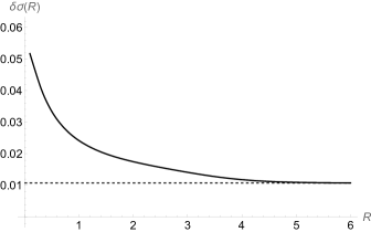
Figure 1: The difference $\delta\sigma({\rm HD},R)$ in ppm of the shielding constant between the deuteron and the proton in HD as a function of the internuclear distance $R$ in a.u. The horizontal line is the separated-atoms limit.

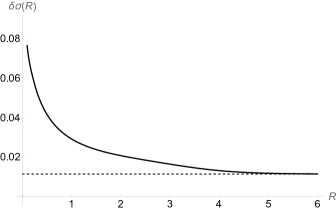
Figure 2: The difference $\delta\sigma({\rm HT},R)$ in ppm of the shielding constant between the triton and the proton in HT as a function of the internuclear distance $R$ in a.u. The horizontal line is the separated-atoms limit.

which yields the following numerical values: $\delta\sigma_{HD}(\infty)\simeq 0.010\,753\cdot 10^{-6}$ and $\delta\sigma_{HT}(\infty)\simeq 0.011\,326\cdot 10^{-6}$. Numerical results in the range $R\in\langle 0.1,6\rangle$ a.u. are collected in Appendix C and presented graphically in Figs 1 and 2, where the correct behavior at the $R\to\infty$ limit can be noted. The final results for the nuclear magnetic shielding constants are obtained by averaging with the nuclear function according to Eq. (21). Apart from checking the consistency with the DNA calculations in the ground energy level, we also obtain the shielding constant differences for excited rotational states, which are populated in 300 K temperature in which the corresponding experiments were performed.

V Results and conclusions

Table 2: Magnetic moment of the deuteron $\mu_{d}$ and the triton $\mu_{t}$ determined from the proton magnetic moment $\mu_{p}$ using Eq. (1). $\mu_{x}({\rm HX})$ denotes the shielded magnetic moment of the nucleus $x$ in the HX molecule. $\Delta_{T}\delta\sigma$ is the change in $\delta\sigma$ caused by the temperature averaging. NAPT results have explicit numerical uncertainties and implicit ones of relative order $3\cdot 10^{-2}$ due to nonadiabatic effects. The uncertainty of the final shielding $\delta\sigma({\rm HX},300K)$ due to relativistic effects is estimated to be $1\cdot 10^{-6}$.

Quantity	Value	Reference
$\mu_{p}$	$2.792\,847\,344\,62(82)\,\mu_{N}$	[1]
$\delta\sigma({\rm HD},v=0,J=0)$	$0.020\,433\cdot 10^{-6}$	NAPT
$\delta\sigma({\rm HD},v=0,J=0)$	$0.019\,901(1)\cdot 10^{-6}$	DNA
$\Delta_{T}\delta\sigma({\rm HD},300K)$	$-0.000\,023\,7\cdot 10^{-6}$	NAPT
$\delta\sigma({\rm HD},300K)$	$0.019\,877(1)\cdot 10^{-6}$	DNA+$\Delta_{T}$
	$0.020\,20(2)\cdot 10^{-6}$	[9]
$\mu_{p}({\rm HD})/\mu_{d}({\rm HD})$	$3.257\,199\,516(10)$	[19, 15]
$\mu_{d}=\mu_{d}({\rm HD})/\mu_{p}({\rm HD})$	$0.857\,438\,233\,8(26)\,\mu_{N}$	This work
$\qquad\times(1+\delta\sigma)\,\mu_{p}$	$0.857\,438\,233\,8(22)\,\mu_{N}$	CODATA [15]
	$0.857\,438\,234\,6(53)\,\mu_{N}$	[9]
$\delta\sigma({\rm HT},v=0,J=0)$	$0.024\,368\cdot 10^{-6}$	NAPT
$\delta\sigma({\rm HT},v=0,J=0)$	$0.023\,975(2)\cdot 10^{-6}$	DNA
$\Delta_{T}\delta\sigma({\rm HT},300K)$	$-0.000\,030\,0\cdot 10^{-6}$	NAPT
$\delta\sigma({\rm HT},300K)$	$0.023\,945(2)\cdot 10^{-6}$	DNA+$\Delta_{T}$
	$0.024\,14(2)\cdot 10^{-6}$	[9]
$\mu_{t}({\rm HT})/\mu_{p}({\rm HT})$	$1.066\,639\,893\,3(21)$	[11, 15]
$\mu_{t}=\mu_{t}({\rm HT})/\mu_{p}({\rm HT})$	$2.978\,962\,465\,0(59)\,\mu_{N}$	This work
$\qquad\times(1+\delta\sigma)\,\mu_{p}$	$2.978\,962\,465\,6(59)\,\mu_{N}$	CODATA [15]
	$2.978\,962\,471(10)\,\mu_{N}$	[9]

Our final numerical results of the deuteron and triton magnetic moments are presented in Table II. As described above, the shielding difference $\delta\sigma=\sigma_{d/t}-\sigma_{p}$ for the ground rovibrational level ($v=0,J=0$) was obtained in two manners; using NAPT, which includes only the leading nonadiabatic effects, and using the DNA method, which completely accounts for the finite nuclear mass effects. The knowledge of the latter enables estimation of the missing higher-order finite-mass effects in the former. The difference NAPT–DNA corresponds to the relative uncertainty of $3\cdot 10^{-2}$ and is consistent with estimation by the square root of the inverse power of the nuclear masses. This difference, however, is an order of magnitude larger than our previous estimation by $m_{\mathrm{e}}/\mu_{\mathrm{n}}\sim 10^{-3}$ in Ref. [9].

The DNA value is augmented by the temperature averaging correction $\Delta_{T}\delta\sigma$ evaluated for $T=300$ kelvins – the temperature in which the measurements were performed. Since it is a quite small effect, for its calculation the adiabatic rotational energies $\varepsilon_{J}$ and wave functions $\chi_{J}$, obtained in the NAPT framework, were employed. First, the shielding difference $\delta\sigma(R)$ was averaged for the lowest 10 rotational states, $\langle\delta\sigma\rangle_{J}=\langle\chi_{J}|\delta\sigma|\chi_{J}\rangle$ and the rotational energies were used to obtain the Boltzmann weights

$$w_{J} =\dfrac{(2J+1)\exp{[-\varepsilon_{J}/(kT)]}}{\sum_{J}(2J+1)\exp{[-\varepsilon_{J}/(kT)]}}.$$ (44)

Then the rotationally averaged $\delta\sigma(R)$ values were summed up with the $J=0$ value subtracted,

$$\Delta_{T}\delta\sigma =\sum_{J}w_{J}\,\langle\delta\sigma\rangle_{J}-\langle\delta\sigma\rangle_{0}\,.$$ (45)

The relative uncertainty of $\Delta_{T}\delta\sigma$ comes mainly from nonadiabatic effects and is about $3\cdot 10^{-2}$, while numerical uncertainty is completely negligible.

The new shielding values slightly differ from our previous result due to underestimation of the nonadiabatic effects and due to mistakes in the final formulas, which we have already discussed. The final shielding difference $\delta\sigma$, labeled ”DNA+$\Delta_{T}$” in Table 2, was used in the evaluation of the magnetic moment of the nucleus $x$ according to

$$\mu_{x}=\mu_{x}({\rm HX})/\mu_{p}({\rm HX})(1+\delta\sigma)\,\mu_{p}$$ (46)

derived directly from Eq. (1).

The obtained values of the deuteron and the triton magnetic moments do not differ greatly from the the CODATA 2018 values which used our previous results. Their accuracy is limited exclusively by experimental uncertainties in the NMR determination of the magnetic moment ratio. In principle, the deuteron and triton magnetic moments can be obtained as accurately as that of the proton, provided the experimental uncertainty in the NMR frequency ratio is reduced by a factor of 10.

Similarly, the magnetic moments of all stable nuclei can, in principle, be determined by a chain of NMR measurements through ³He. The ³He magnetic moment can be obtained by measuring the magnetic moment ratio in H₂ and ³He. For this, one would need nonadiabatic shielding and relativistic correction in H₂, while for ³He the shielding is already accurately known [2]. The nonadiabatic shielding in H₂ and other molecules can be calculated by means of the DNA method or NAPT, as presented in this work, while relativistic corrections are yet to be calculated in a similar way as for ³He. Such results would eventually allow for much-improved determination of all the nuclear magnetic moments.

Appendix A Operator matrix element in NAPT

Although most of the consideration below will be valid for an arbitrary molecule, to be more specific, we consider a two-electron diatomic molecule. The total wave function $\psi$ is a solution of the stationary Schrödinger equation

$$H_{0}\,\Psi=E\,\Psi\,,$$ (47)

with the Hamiltonian

$$H_{0}=H_{\rm el}+H_{\rm n}\,,$$ (48)

split into the electronic and nuclear parts. In the electronic Hamiltonian

$$H_{\rm el}=-\sum_{a}\frac{\nabla^{2}_{a}}{2\,m_{\mathrm{e}}}+V\,,$$ (49)

where $V$ is the Coulomb interaction potential

$$V=-\frac{1}{r_{1A}}-\frac{1}{r_{1B}}-\frac{1}{r_{2A}}-\frac{1}{r_{2B}}+\frac{1}{r_{12}}+\frac{1}{R},$$ (50)

the nuclei have fixed positions $\vec{R}_{A}$ (proton) and $\vec{R}_{B}$ (deuteron/triton), and $\vec{R}=\vec{R}_{A}-\vec{R}_{B}$. The nuclear Hamiltonian is

$$H_{\rm n}= \ -\frac{\nabla_{A}^{2}}{2\,m_{A}}-\frac{\nabla_{B}^{2}}{2\,m_{B}}\,.$$ (51)

Because $m/m_{A}$ and $m/m_{B}$ are small, it is customary to assume that the total wave function of the molecule

$$\psi(\vec{r},\vec{R})=\phi(\vec{r};\,\vec{R})\;\chi(\vec{R})$$ (52)

is a product of the electronic wave function $\phi$ that depends parametrically on $R$, and the nuclear wave function $\chi$. The electronic wave function obeys the clamped nuclei electronic Schrödinger equation

$$\bigl{[}H_{\rm el}-\mathcal{E}_{\mathrm{el}}(R)\bigr{]}\,|\phi\rangle=0,$$ (53)

while the wave function $\chi$ is a solution to the nuclear Schrödinger equation with the effective potential generated by electrons

$$({\cal H}-E)\,|\chi\rangle=0\,,$$ (54)

where

$${\cal H} =-\frac{\vec{\nabla}_{R}^{2}}{2\,\mu_{\mathrm{n}}}+\mathcal{E}_{\mathrm{a}}(R)+\mathcal{E}_{\mathrm{el}}(R).$$ (55)

The function

$$\mathcal{E}_{\mathrm{a}}(R)=\left\langle\phi\left|H_{\rm n}\right|\phi\right\rangle_{\!\mathrm{el}}$$ (56)

is the so-called adiabatic correction, where the subscript ”el” is explained in the following. We shall consider two different types of matrix elements of an operator $\Omega$ containing differentiation over $R$, which differ in the range of differentiation. The first type of the matrix element

$$\langle\phi^{\prime}|\Omega|\phi\rangle$$ (57)

will be understood as an operator acting in the subspace of rotational and vibrational states $\chi$

$$\langle\chi^{\prime}|\langle\phi^{\prime}|\Omega|\phi\rangle|\chi\rangle\,,$$ (58)

which means that $\Omega$ acts on both $\phi$ and $\chi$. The second type of the matrix element

$$\langle\phi^{\prime}|\Omega|\phi\rangle_{\mathrm{el}}\,,$$ (59)

distinguished by the subscript ”el”, has the differentiation range limited to the single function $\phi$ immediately following $\Omega$. For example,

$$\langle\phi^{\prime}|\vec{\nabla}_{\!R}|\phi\rangle_{\mathrm{el}}=\langle\phi^{\prime}|\vec{\nabla}_{\!R}\phi\rangle\,.$$ (60)

To shorten the forthcoming expressions, we define the ”left-hand” differential operator,

$$\langle\phi^{\prime}|\mathchoice{\mkern 3.0mu\reflectbox{$\displaystyle\vec{\reflectbox{$\mkern-3.0mu\displaystyle\nabla\mkern 3.0mu$}}$}\mkern-3.0mu}{\mkern 3.0mu\reflectbox{$\textstyle\vec{\reflectbox{$\mkern-3.0mu\textstyle\nabla\mkern 3.0mu$}}$}\mkern-3.0mu}{\mkern 2.0mu\reflectbox{$\scriptstyle\vec{\reflectbox{$\mkern-2.0mu\scriptstyle\nabla\mkern 2.0mu$}}$}\mkern-2.0mu}{\mkern 2.0mu\reflectbox{$\scriptscriptstyle\vec{\reflectbox{$\mkern-2.0mu\scriptscriptstyle\nabla\mkern 2.0mu$}}$}\mkern-2.0mu}_{\!R}|\phi\rangle_{\mathrm{el}}=\langle\vec{\nabla}_{\!R}\phi^{\prime}|\phi\rangle.$$ (61)

For a clear definition of the scope of action of the $R$ derivative, we introduce another symbol

$$\vec{\nabla}_{\!R}[Q]\equiv[\vec{\nabla}_{\!R},Q]\,.$$ (62)

For example, for arbitrary states $\phi^{\prime}$, $\phi$, we have

$$\vec{\nabla}_{\!R}[\langle\phi^{\prime}|\phi\rangle] =\langle\phi^{\prime}|\mathchoice{\mkern 3.0mu\reflectbox{$\displaystyle\vec{\reflectbox{$\mkern-3.0mu\displaystyle\nabla\mkern 3.0mu$}}$}\mkern-3.0mu}{\mkern 3.0mu\reflectbox{$\textstyle\vec{\reflectbox{$\mkern-3.0mu\textstyle\nabla\mkern 3.0mu$}}$}\mkern-3.0mu}{\mkern 2.0mu\reflectbox{$\scriptstyle\vec{\reflectbox{$\mkern-2.0mu\scriptstyle\nabla\mkern 2.0mu$}}$}\mkern-2.0mu}{\mkern 2.0mu\reflectbox{$\scriptscriptstyle\vec{\reflectbox{$\mkern-2.0mu\scriptscriptstyle\nabla\mkern 2.0mu$}}$}\mkern-2.0mu}_{\!R}+\vec{\nabla}_{\!R}|\phi\rangle_{\mathrm{el}}\,.$$ (63)

If these states are orthogonal $\langle\phi^{\prime}|\phi\rangle=0$, then

$$\langle\phi^{\prime}|\mathchoice{\mkern 3.0mu\reflectbox{$\displaystyle\vec{\reflectbox{$\mkern-3.0mu\displaystyle\nabla\mkern 3.0mu$}}$}\mkern-3.0mu}{\mkern 3.0mu\reflectbox{$\textstyle\vec{\reflectbox{$\mkern-3.0mu\textstyle\nabla\mkern 3.0mu$}}$}\mkern-3.0mu}{\mkern 2.0mu\reflectbox{$\scriptstyle\vec{\reflectbox{$\mkern-2.0mu\scriptstyle\nabla\mkern 2.0mu$}}$}\mkern-2.0mu}{\mkern 2.0mu\reflectbox{$\scriptscriptstyle\vec{\reflectbox{$\mkern-2.0mu\scriptscriptstyle\nabla\mkern 2.0mu$}}$}\mkern-2.0mu}_{\!R}+\vec{\nabla}_{\!R}|\phi\rangle_{\mathrm{el}}=0$$ (64)

and the left- and right-hand derivatives differ by sign. If, in turn, $\phi^{\prime}=\phi$ and $\phi$ is a normalized real function $(\langle\phi|\phi\rangle=1)$, then these derivatives vanish,

$$\langle\phi|\mathchoice{\mkern 3.0mu\reflectbox{$\displaystyle\vec{\reflectbox{$\mkern-3.0mu\displaystyle\nabla\mkern 3.0mu$}}$}\mkern-3.0mu}{\mkern 3.0mu\reflectbox{$\textstyle\vec{\reflectbox{$\mkern-3.0mu\textstyle\nabla\mkern 3.0mu$}}$}\mkern-3.0mu}{\mkern 2.0mu\reflectbox{$\scriptstyle\vec{\reflectbox{$\mkern-2.0mu\scriptstyle\nabla\mkern 2.0mu$}}$}\mkern-2.0mu}{\mkern 2.0mu\reflectbox{$\scriptscriptstyle\vec{\reflectbox{$\mkern-2.0mu\scriptscriptstyle\nabla\mkern 2.0mu$}}$}\mkern-2.0mu}_{R}|\phi\rangle_{\mathrm{el}}=\langle\phi|\vec{\nabla}_{R}|\phi\rangle_{\mathrm{el}}=0\,.$$ (65)

Therefore, for these states the matrix element of the nuclear kinetic energy is

$$\langle\phi|\vec{\nabla}_{R}^{2}|\phi\rangle= \ \vec{\nabla}_{R}^{2}+\langle\phi|\vec{\nabla}_{R}^{2}|\phi\rangle_{\mathrm{el}}$$

$$= \ \vec{\nabla}_{R}^{2}-\langle\phi|\mathchoice{\mkern 3.0mu\reflectbox{$\displaystyle\vec{\reflectbox{$\mkern-3.0mu\displaystyle\nabla\mkern 3.0mu$}}$}\mkern-3.0mu}{\mkern 3.0mu\reflectbox{$\textstyle\vec{\reflectbox{$\mkern-3.0mu\textstyle\nabla\mkern 3.0mu$}}$}\mkern-3.0mu}{\mkern 2.0mu\reflectbox{$\scriptstyle\vec{\reflectbox{$\mkern-2.0mu\scriptstyle\nabla\mkern 2.0mu$}}$}\mkern-2.0mu}{\mkern 2.0mu\reflectbox{$\scriptscriptstyle\vec{\reflectbox{$\mkern-2.0mu\scriptscriptstyle\nabla\mkern 2.0mu$}}$}\mkern-2.0mu}_{R}\,\vec{\nabla}_{R}|\phi\rangle_{\mathrm{el}}\,,$$ (66)

which explains the form of the nuclear Hamiltonian in Eq. (55).

We will be using the following type of matrix element with arbitrary real functions $\phi$ and $\phi^{\prime}$:

$$\vec{Z}\equiv\langle\phi^{\prime}|\vec{\nabla}_{R}|\phi\rangle+\langle\phi|\mathchoice{\mkern 3.0mu\reflectbox{$\displaystyle\vec{\reflectbox{$\mkern-3.0mu\displaystyle\nabla\mkern 3.0mu$}}$}\mkern-3.0mu}{\mkern 3.0mu\reflectbox{$\textstyle\vec{\reflectbox{$\mkern-3.0mu\textstyle\nabla\mkern 3.0mu$}}$}\mkern-3.0mu}{\mkern 2.0mu\reflectbox{$\scriptstyle\vec{\reflectbox{$\mkern-2.0mu\scriptstyle\nabla\mkern 2.0mu$}}$}\mkern-2.0mu}{\mkern 2.0mu\reflectbox{$\scriptscriptstyle\vec{\reflectbox{$\mkern-2.0mu\scriptscriptstyle\nabla\mkern 2.0mu$}}$}\mkern-2.0mu}_{R}|\phi^{\prime}\rangle.$$ (67)

This expression can be transformed as follows:

$$\vec{Z}= \ \langle\phi^{\prime}|\vec{\nabla}_{R}|\phi\rangle_{\rm el}+\langle\phi|\mathchoice{\mkern 3.0mu\reflectbox{$\displaystyle\vec{\reflectbox{$\mkern-3.0mu\displaystyle\nabla\mkern 3.0mu$}}$}\mkern-3.0mu}{\mkern 3.0mu\reflectbox{$\textstyle\vec{\reflectbox{$\mkern-3.0mu\textstyle\nabla\mkern 3.0mu$}}$}\mkern-3.0mu}{\mkern 2.0mu\reflectbox{$\scriptstyle\vec{\reflectbox{$\mkern-2.0mu\scriptstyle\nabla\mkern 2.0mu$}}$}\mkern-2.0mu}{\mkern 2.0mu\reflectbox{$\scriptscriptstyle\vec{\reflectbox{$\mkern-2.0mu\scriptscriptstyle\nabla\mkern 2.0mu$}}$}\mkern-2.0mu}_{R}|\phi^{\prime}\rangle_{\rm el}+\langle\phi^{\prime}|\phi\rangle\,\vec{\nabla}_{R}+\mathchoice{\mkern 3.0mu\reflectbox{$\displaystyle\vec{\reflectbox{$\mkern-3.0mu\displaystyle\nabla\mkern 3.0mu$}}$}\mkern-3.0mu}{\mkern 3.0mu\reflectbox{$\textstyle\vec{\reflectbox{$\mkern-3.0mu\textstyle\nabla\mkern 3.0mu$}}$}\mkern-3.0mu}{\mkern 2.0mu\reflectbox{$\scriptstyle\vec{\reflectbox{$\mkern-2.0mu\scriptstyle\nabla\mkern 2.0mu$}}$}\mkern-2.0mu}{\mkern 2.0mu\reflectbox{$\scriptscriptstyle\vec{\reflectbox{$\mkern-2.0mu\scriptscriptstyle\nabla\mkern 2.0mu$}}$}\mkern-2.0mu}_{R}\,\langle\phi|\phi^{\prime}\rangle$$

$$= \ 2\,\langle\phi^{\prime}|\vec{\nabla}_{R}|\phi\rangle_{\rm el}-[\vec{\nabla}_{R}\,,\,\langle\phi^{\prime}|\phi\rangle]$$

$$= \ \langle\phi^{\prime}|\vec{\nabla}_{R}-\mathchoice{\mkern 3.0mu\reflectbox{$\displaystyle\vec{\reflectbox{$\mkern-3.0mu\displaystyle\nabla\mkern 3.0mu$}}$}\mkern-3.0mu}{\mkern 3.0mu\reflectbox{$\textstyle\vec{\reflectbox{$\mkern-3.0mu\textstyle\nabla\mkern 3.0mu$}}$}\mkern-3.0mu}{\mkern 2.0mu\reflectbox{$\scriptstyle\vec{\reflectbox{$\mkern-2.0mu\scriptstyle\nabla\mkern 2.0mu$}}$}\mkern-2.0mu}{\mkern 2.0mu\reflectbox{$\scriptscriptstyle\vec{\reflectbox{$\mkern-2.0mu\scriptscriptstyle\nabla\mkern 2.0mu$}}$}\mkern-2.0mu}_{R}|\phi\rangle_{\rm el}$$ (68)

If, additionally, $\langle\phi^{\prime}|\phi\rangle=0$, then $\vec{Z}=2\,\langle\phi^{\prime}|\vec{\nabla}_{\!R}|\phi\rangle_{\rm el}$.

In the reference frame attached to the geometrical center of the nuclei, $H_{\rm n}$ can be written as a sum of two components,

$$H^{\prime}_{\rm n}= \ -\frac{\nabla^{2}_{\!R}}{2\,\mu_{\mathrm{n}}}-\frac{{\nabla}_{\!\mathrm{el}}^{2}}{8\,\mu_{\mathrm{n}}}$$ (69)

$$H^{\prime\prime}_{\rm n}= \ \frac{1}{2}\biggl{(}\frac{1}{M_{A}}-\frac{1}{M_{B}}\biggr{)}\,\vec{\nabla}_{R}\cdot\vec{\nabla}_{\!\mathrm{el}}$$ (70)

with the first one being even and the second- one being odd with respect to the inversion. In the above $\vec{\nabla}_{\!\mathrm{el}}=\sum_{a}\vec{\nabla}_{\!a}$ and $\mu_{\mathrm{n}}=\left(1/M_{A}+1/M_{B}\right)^{-1}$ is the reduced nuclear mass. Due to the inversion symmetry of $\phi$ with respect to the geometrical center, $\langle\phi|H^{\prime\prime}_{\rm n}|\phi\rangle_{\rm el}=0$ and

$$\mathcal{E}_{\mathrm{a}}(R) =\left\langle\phi\left|H^{\prime}_{\rm n}\right|\phi\right\rangle_{\!\mathrm{el}}$$

$$=\frac{1}{2\,\mu_{\mathrm{n}}}\,\left\langle\phi\left|\mathchoice{\mkern 3.0mu\reflectbox{$\displaystyle\vec{\reflectbox{$\mkern-3.0mu\displaystyle\nabla\mkern 3.0mu$}}$}\mkern-3.0mu}{\mkern 3.0mu\reflectbox{$\textstyle\vec{\reflectbox{$\mkern-3.0mu\textstyle\nabla\mkern 3.0mu$}}$}\mkern-3.0mu}{\mkern 2.0mu\reflectbox{$\scriptstyle\vec{\reflectbox{$\mkern-2.0mu\scriptstyle\nabla\mkern 2.0mu$}}$}\mkern-2.0mu}{\mkern 2.0mu\reflectbox{$\scriptscriptstyle\vec{\reflectbox{$\mkern-2.0mu\scriptscriptstyle\nabla\mkern 2.0mu$}}$}\mkern-2.0mu}_{R}\cdot\vec{\nabla}_{R}\right|\phi\right\rangle_{\rm el}-\frac{1}{8\,\mu_{\mathrm{n}}}\left\langle\phi\left|\vec{\nabla}_{\!\mathrm{el}}^{2}\right|\phi\right\rangle.$$ (71)

However, for the determination of the difference in the shielding of the proton and deuteron magnetic moments, we shall consider the reference frame centered on one of the nuclei, say nucleus $A$. The nuclear Hamiltonian then becomes

$$H_{\rm n}= \ -\frac{(\vec{\nabla}_{B}+\vec{\nabla}_{\rm el})^{2}}{2\,m_{A}}-\frac{\vec{\nabla}_{B}^{2}}{2\,m_{B}}$$

$$= \ H^{\prime}_{\rm n}+H^{\prime\prime}_{\rm n}$$ (72)

where

$$H^{\prime}_{\rm n}= \ -\frac{\vec{\nabla}_{B}^{2}}{2\,\mu_{\mathrm{n}}}$$ (73)

$$H^{\prime\prime}_{\rm n}= \ -\frac{\vec{\nabla}_{\rm el}^{2}}{2\,m_{A}}-\frac{\vec{\nabla}_{\!\mathrm{el}}\cdot\vec{\nabla}_{\!B}}{m_{A}}\,.$$ (74)

Vectors with the origin at $A$, pointing at a particle $a$ will be denoted by $\vec{x}_{a}$, and $\vec{\nabla}_{\!B}\equiv-\vec{\nabla}_{\!R}$. The diagonal matrix element of $H^{\prime}_{\rm n}$

$$\langle\phi|H^{\prime}_{\rm n}|\phi\rangle_{\rm el}=\frac{1}{2\,\mu_{\mathrm{n}}}\,\langle\phi|\mathchoice{\mkern 3.0mu\reflectbox{$\displaystyle\vec{\reflectbox{$\mkern-3.0mu\displaystyle\nabla\mkern 3.0mu$}}$}\mkern-3.0mu}{\mkern 3.0mu\reflectbox{$\textstyle\vec{\reflectbox{$\mkern-3.0mu\textstyle\nabla\mkern 3.0mu$}}$}\mkern-3.0mu}{\mkern 2.0mu\reflectbox{$\scriptstyle\vec{\reflectbox{$\mkern-2.0mu\scriptstyle\nabla\mkern 2.0mu$}}$}\mkern-2.0mu}{\mkern 2.0mu\reflectbox{$\scriptscriptstyle\vec{\reflectbox{$\mkern-2.0mu\scriptscriptstyle\nabla\mkern 2.0mu$}}$}\mkern-2.0mu}_{\!B}\cdot\vec{\nabla}_{\!B}|\phi\rangle_{\rm el}\,.$$ (75)

This term does not contribute to the difference in the nuclear magnetic shielding because it depends on the reduced nuclear mass only. The diagonal matrix element of the second term in $H^{\prime\prime}_{\rm n}$ is

$$\delta\cal{E} =-\frac{1}{m_{A}}\,\langle\phi|\vec{\nabla}_{\!\mathrm{el}}\cdot\vec{\nabla}_{\!B}|\phi\rangle_{\mathrm{el}}\,.$$ (76)

By acting $\vec{\nabla}_{B}$ on the Schrödinger equation (53), $\delta\cal{E}$ can be transformed to

$$\delta\cal{E} =-\frac{1}{m_{A}}\,\langle\phi|\vec{\nabla}_{\!\mathrm{el}}\frac{1}{({\cal E}_{\rm el}-H_{\rm el})^{\prime}}\vec{\nabla}_{\!B}[V-{\cal E}_{\rm el}]|\phi\rangle\,,$$ (77)

where the notation introduced in Eq. (62) was applied. To make formulas more compact, we now introduce an abbreviated notation $\langle\dots\rangle\equiv\langle\phi|\dots|\phi\rangle$. Because $\vec{\nabla}_{\!\mathrm{el}}=m_{\mathrm{e}}\,[\vec{x}_{\rm el}\,,\,H_{\rm el}]$, where $\vec{x}_{\rm el}=\sum_{a}\vec{x}_{a}$, the expectation value (77) can be rewritten as

$$\delta{\cal E} =\frac{m_{\mathrm{e}}}{m_{A}}\,\langle[\vec{x}_{\rm el}\,,\,{\cal E}_{\rm el}-H_{\rm el}]\frac{1}{({\cal E}_{\rm el}-H_{\rm el})^{\prime}}\vec{\nabla}_{\!B}[V-{\cal E}_{\rm el}]\rangle$$

$$=\frac{m_{\mathrm{e}}}{m_{A}}\,\langle\vec{x}_{\rm el}\,(I-|\phi\rangle\,\langle\phi|)\,\vec{\nabla}_{\!B}[V-{\cal E}_{\rm el}]\rangle$$

$$=\frac{m_{\mathrm{e}}}{m_{A}}\,\langle\left(\vec{x}_{\rm el}-\langle\vec{x}_{\mathrm{el}}\rangle\right)\,\vec{\nabla}_{\!B}[V-{\cal E}_{\rm el}]\rangle$$ (78)

and we note that $\langle\vec{\nabla}_{\!B}[V-{\cal E}_{\rm el}]\rangle=0$. It is convenient to define the following operator

$$\tilde{H}_{\rm n}\equiv(\vec{x}_{\rm el}-\langle\vec{x}_{\mathrm{el}}\rangle)\,\vec{\nabla}_{\!B}[V-{\cal E}_{\rm el}]-\frac{\vec{\nabla}_{\rm el}^{2}}{2\,m_{\mathrm{e}}}\,,$$ (79)

which will be used in the calculation of the shielding constant difference. Because the adiabatic energy does not depend on the reference frame, the diagonal matrix element of $\tilde{H}_{\rm n}$, with $\langle\vec{x}_{\mathrm{el}}\rangle=-\vec{R}$, vanishes:

$$\langle\phi|H^{\prime\prime}_{\rm n}|\phi\rangle_{\rm el}=\frac{m_{\mathrm{e}}}{m_{A}}\,\langle\tilde{H}_{\rm n}\rangle=0\,,$$ (80)

which can be shown by replacing $\vec{\nabla}_{B}=(\vec{\nabla}_{A}+\vec{\nabla}_{B})/2+(\vec{\nabla}_{B}-\vec{\nabla}_{A})/2$. The expectation value of $\tilde{H}_{\rm n}$ with the second term vanishes because the ground state has gerade symmetry, while the first term can be replaced by $-\vec{\nabla}_{\rm el}/2$; hence,

$$\langle\tilde{H}_{\rm n}\rangle =\left\langle-\frac{1}{2}(\vec{x}_{\rm el}-\langle\vec{x}_{\mathrm{el}}\rangle)\,[\vec{\nabla}_{\rm el}\,,\,H_{\rm el}-{\cal E}_{\rm el}]-\frac{\vec{\nabla}_{\rm el}^{2}}{2\,m_{\mathrm{e}}}\right\rangle$$

$$=\left\langle\frac{1}{2}[\vec{x}_{\rm el}-\langle\vec{x}_{\mathrm{el}}\rangle\,,\,H_{\rm el}-{\cal E}_{\rm el}]\cdot\,\vec{\nabla}_{\rm el}-\frac{\vec{\nabla}_{\rm el}^{2}}{2\,m_{\mathrm{e}}}\right\rangle=0\,.$$ (81)

Appendix B Derivation of finite nuclear mass corrections $\sigma_{\rm n}$

The shielding correction $\sigma_{\rm n}$ is obtained from the leading one by correcting all matrix elements by $H^{\prime\prime}_{\rm n}$ in Eq. (74), and it is split into two terms, i.e., $\sigma_{\rm n}=\sigma_{\mathrm{n1}}+\sigma_{\mathrm{n2}}$. Consider the finite nuclear mass corrections to the first BO term

$$\sigma_{\mathrm{n1}}= \ \frac{\alpha^{2}}{3}\,\biggl{[}\Big{\langle}Q_{0}\,\frac{1}{({\cal E}_{\rm el}-H_{\rm el})^{\prime}}\,{H^{\prime\prime}_{\rm n}}\Big{\rangle}+\Big{\langle}{H^{\prime\prime}_{\rm n}}\,\frac{1}{({\cal E}_{\rm el}-H_{\rm el})^{\prime}}\,Q_{0}\Big{\rangle}\biggr{]},$$ (82)

where

$$Q_{0}=\sum_{b}\frac{1}{x_{b}}.$$ (83)

$\vec{\nabla}_{\rm el}^{2}$, the first term in $H^{\prime\prime}_{\rm n}$ of Eq. (74), does not need any further transformation, while the second term does:

$${\delta\sigma_{\mathrm{n1}}}= \ -\frac{\alpha^{2}}{3\,m_{A}}\,\biggl{[}\Big{\langle}Q_{0}\,\frac{1}{({\cal E}_{\rm el}-H_{\rm el})^{\prime}}\,\vec{\nabla}_{B}\vec{\nabla}_{\rm el}\Big{\rangle}$$

$$\ +\Big{\langle}\mathchoice{\mkern 3.0mu\reflectbox{$\displaystyle\vec{\reflectbox{$\mkern-3.0mu\displaystyle\nabla\mkern 3.0mu$}}$}\mkern-3.0mu}{\mkern 3.0mu\reflectbox{$\textstyle\vec{\reflectbox{$\mkern-3.0mu\textstyle\nabla\mkern 3.0mu$}}$}\mkern-3.0mu}{\mkern 2.0mu\reflectbox{$\scriptstyle\vec{\reflectbox{$\mkern-2.0mu\scriptstyle\nabla\mkern 2.0mu$}}$}\mkern-2.0mu}{\mkern 2.0mu\reflectbox{$\scriptscriptstyle\vec{\reflectbox{$\mkern-2.0mu\scriptscriptstyle\nabla\mkern 2.0mu$}}$}\mkern-2.0mu}_{B}\mathchoice{\mkern 3.0mu\reflectbox{$\displaystyle\vec{\reflectbox{$\mkern-3.0mu\displaystyle\nabla\mkern 3.0mu$}}$}\mkern-3.0mu}{\mkern 3.0mu\reflectbox{$\textstyle\vec{\reflectbox{$\mkern-3.0mu\textstyle\nabla\mkern 3.0mu$}}$}\mkern-3.0mu}{\mkern 2.0mu\reflectbox{$\scriptstyle\vec{\reflectbox{$\mkern-2.0mu\scriptstyle\nabla\mkern 2.0mu$}}$}\mkern-2.0mu}{\mkern 2.0mu\reflectbox{$\scriptscriptstyle\vec{\reflectbox{$\mkern-2.0mu\scriptscriptstyle\nabla\mkern 2.0mu$}}$}\mkern-2.0mu}_{\rm el}\,\frac{1}{({\cal E}_{\rm el}-H_{\rm el})^{\prime}}\,Q_{0}\Big{\rangle}\biggr{]}.$$ (84)

This is the $Z$ type matrix element, so

$${\delta\sigma_{\mathrm{n1}}}= \ -\frac{\alpha^{2}}{3\,m_{A}}\,\Big{\langle}Q_{0}\,\frac{1}{({\cal E}_{\rm el}-H_{\rm el})^{\prime}}\,(\vec{\nabla}_{B}-\mathchoice{\mkern 3.0mu\reflectbox{$\displaystyle\vec{\reflectbox{$\mkern-3.0mu\displaystyle\nabla\mkern 3.0mu$}}$}\mkern-3.0mu}{\mkern 3.0mu\reflectbox{$\textstyle\vec{\reflectbox{$\mkern-3.0mu\textstyle\nabla\mkern 3.0mu$}}$}\mkern-3.0mu}{\mkern 2.0mu\reflectbox{$\scriptstyle\vec{\reflectbox{$\mkern-2.0mu\scriptstyle\nabla\mkern 2.0mu$}}$}\mkern-2.0mu}{\mkern 2.0mu\reflectbox{$\scriptscriptstyle\vec{\reflectbox{$\mkern-2.0mu\scriptscriptstyle\nabla\mkern 2.0mu$}}$}\mkern-2.0mu}_{B})\vec{\nabla}_{\rm el}\Big{\rangle}_{\rm el}$$

$$= \ -\frac{\alpha^{2}\,m}{3\,m_{A}}\Big{\langle}Q_{0}\,\frac{1}{({\cal E}_{\rm el}-H_{\rm el})^{\prime}}\,[{\cal E}_{\rm el}-H_{\rm el}\,,\,\vec{x}_{\rm el}-\langle\vec{x}_{\rm el}\rangle]\,(\vec{\nabla}_{B}-\mathchoice{\mkern 3.0mu\reflectbox{$\displaystyle\vec{\reflectbox{$\mkern-3.0mu\displaystyle\nabla\mkern 3.0mu$}}$}\mkern-3.0mu}{\mkern 3.0mu\reflectbox{$\textstyle\vec{\reflectbox{$\mkern-3.0mu\textstyle\nabla\mkern 3.0mu$}}$}\mkern-3.0mu}{\mkern 2.0mu\reflectbox{$\scriptstyle\vec{\reflectbox{$\mkern-2.0mu\scriptstyle\nabla\mkern 2.0mu$}}$}\mkern-2.0mu}{\mkern 2.0mu\reflectbox{$\scriptscriptstyle\vec{\reflectbox{$\mkern-2.0mu\scriptscriptstyle\nabla\mkern 2.0mu$}}$}\mkern-2.0mu}_{B})\Big{\rangle}_{\rm el}$$

$$= \ -\frac{\alpha^{2}\,m}{3\,m_{A}}\Big{\langle}\bigl{(}Q_{0}-\bigl{\langle}Q_{0}\bigr{\rangle}\bigr{)}\,(\vec{x}_{\rm el}-\langle\vec{x}_{\rm el}\rangle)\,(\vec{\nabla}_{B}-\mathchoice{\mkern 3.0mu\reflectbox{$\displaystyle\vec{\reflectbox{$\mkern-3.0mu\displaystyle\nabla\mkern 3.0mu$}}$}\mkern-3.0mu}{\mkern 3.0mu\reflectbox{$\textstyle\vec{\reflectbox{$\mkern-3.0mu\textstyle\nabla\mkern 3.0mu$}}$}\mkern-3.0mu}{\mkern 2.0mu\reflectbox{$\scriptstyle\vec{\reflectbox{$\mkern-2.0mu\scriptstyle\nabla\mkern 2.0mu$}}$}\mkern-2.0mu}{\mkern 2.0mu\reflectbox{$\scriptscriptstyle\vec{\reflectbox{$\mkern-2.0mu\scriptscriptstyle\nabla\mkern 2.0mu$}}$}\mkern-2.0mu}_{B})\Big{\rangle}_{\rm el}+\frac{\alpha^{2}\,m}{3\,m_{A}}\Big{\langle}Q_{0}\,\frac{1}{({\cal E}_{\rm el}-H_{\rm el})^{\prime}}\,(\vec{x}_{\rm el}-\langle\vec{x}_{\rm el})\,[{\cal E}_{\rm el}-H_{\rm el}\,,\,\vec{\nabla}_{B}-\mathchoice{\mkern 3.0mu\reflectbox{$\displaystyle\vec{\reflectbox{$\mkern-3.0mu\displaystyle\nabla\mkern 3.0mu$}}$}\mkern-3.0mu}{\mkern 3.0mu\reflectbox{$\textstyle\vec{\reflectbox{$\mkern-3.0mu\textstyle\nabla\mkern 3.0mu$}}$}\mkern-3.0mu}{\mkern 2.0mu\reflectbox{$\scriptstyle\vec{\reflectbox{$\mkern-2.0mu\scriptstyle\nabla\mkern 2.0mu$}}$}\mkern-2.0mu}{\mkern 2.0mu\reflectbox{$\scriptscriptstyle\vec{\reflectbox{$\mkern-2.0mu\scriptscriptstyle\nabla\mkern 2.0mu$}}$}\mkern-2.0mu}_{B}]\Big{\rangle}_{\rm el}$$

$$= \ \frac{2\,\alpha^{2}\,m}{3\,m_{A}}\Big{\langle}Q_{0}\,\frac{1}{({\cal E}_{\rm el}-H_{\rm el})^{\prime}}\,(\vec{x}_{\rm el}-\langle\vec{x}_{\rm el})\,\vec{\nabla}_{B}[V-\cal{E}_{\rm el}]\Big{\rangle}\,.$$ (85)

Therefore,

$$\sigma_{\mathrm{n1}}= \ \frac{2\,\alpha^{2}}{3\,m_{A}}\langle\phi|Q_{0}\,\frac{1}{({\cal E}_{\rm el}-H_{\rm el})^{\prime}}\,{\tilde{H}}_{\rm n}|\phi\rangle\,.$$ (86)

Consider now the finite nuclear mass corrections to the second BO term, and let

$$\vec{Q}_{1}= \ \sum_{a}\vec{x}_{a}\times\vec{p}_{a},\qquad\langle\vec{Q}_{1}\rangle=0,$$ (87)

$$\vec{Q}_{2}= \ \sum_{b}\frac{\vec{x}_{b}\times\vec{p}_{b}}{x_{b}^{3}},\qquad\langle\vec{Q}_{2}\rangle=0\,.$$ (88)

Then

$$\sigma_{\mathrm{n2}}= \ \frac{\alpha^{2}}{3}\,\biggl{[}\Big{\langle}{H^{\prime\prime}_{\rm n}}\,\frac{1}{({\cal E}_{\rm el}-H_{\rm el})^{\prime}}\,\vec{Q}_{1}\frac{1}{({\cal E}_{\rm el}-H_{\rm el})^{\prime}}\vec{Q}_{2}\Big{\rangle}+\Big{\langle}\vec{Q}_{1}\frac{1}{({\cal E}_{\rm el}-H_{\rm el})^{\prime}}\,H^{\prime\prime}_{\rm n}\frac{1}{({\cal E}_{\rm el}-H_{\rm el})^{\prime}}\,\vec{Q}_{2}\Big{\rangle}$$

$$\ +\Big{\langle}\vec{Q}_{1}\,\frac{1}{({\cal E}_{\rm el}-H_{\rm el})^{\prime}}\,\vec{Q}_{2}\,\frac{1}{({\cal E}_{\rm el}-H_{\rm el})^{\prime}}\,{H^{\prime\prime}_{\rm n}}\Big{\rangle}\biggr{]}.$$ (89)

One notes that the matrix element due to the second term in $H^{\prime\prime}_{\rm n}$ is of the $Z$-type, so

$${\delta\sigma_{\mathrm{n2}}}= \ -\frac{\alpha^{2}}{6\,m_{A}}\,\biggl{[}\Big{\langle}(\vec{\nabla}_{B}-\mathchoice{\mkern 3.0mu\reflectbox{$\displaystyle\vec{\reflectbox{$\mkern-3.0mu\displaystyle\nabla\mkern 3.0mu$}}$}\mkern-3.0mu}{\mkern 3.0mu\reflectbox{$\textstyle\vec{\reflectbox{$\mkern-3.0mu\textstyle\nabla\mkern 3.0mu$}}$}\mkern-3.0mu}{\mkern 2.0mu\reflectbox{$\scriptstyle\vec{\reflectbox{$\mkern-2.0mu\scriptstyle\nabla\mkern 2.0mu$}}$}\mkern-2.0mu}{\mkern 2.0mu\reflectbox{$\scriptscriptstyle\vec{\reflectbox{$\mkern-2.0mu\scriptscriptstyle\nabla\mkern 2.0mu$}}$}\mkern-2.0mu}_{B})\,\vec{\nabla}_{\rm el}\,\frac{1}{({\cal E}_{\rm el}-H_{\rm el})^{\prime}}\,\vec{Q}_{1}\frac{1}{({\cal E}_{\rm el}-H_{\rm el})^{\prime}}\vec{Q}_{2}\Big{\rangle}_{\rm el}+\Big{\langle}\vec{Q}_{1}\frac{1}{({\cal E}_{\rm el}-H_{\rm el})^{\prime}}\,(\vec{\nabla}_{B}-\mathchoice{\mkern 3.0mu\reflectbox{$\displaystyle\vec{\reflectbox{$\mkern-3.0mu\displaystyle\nabla\mkern 3.0mu$}}$}\mkern-3.0mu}{\mkern 3.0mu\reflectbox{$\textstyle\vec{\reflectbox{$\mkern-3.0mu\textstyle\nabla\mkern 3.0mu$}}$}\mkern-3.0mu}{\mkern 2.0mu\reflectbox{$\scriptstyle\vec{\reflectbox{$\mkern-2.0mu\scriptstyle\nabla\mkern 2.0mu$}}$}\mkern-2.0mu}{\mkern 2.0mu\reflectbox{$\scriptscriptstyle\vec{\reflectbox{$\mkern-2.0mu\scriptscriptstyle\nabla\mkern 2.0mu$}}$}\mkern-2.0mu}_{B})\,\vec{\nabla}_{\rm el}\,\frac{1}{({\cal E}_{\rm el}-H_{\rm el})^{\prime}}\,\vec{Q}_{2}\Big{\rangle}_{\rm el}$$

$$\ +\Big{\langle}\vec{Q}_{1}\,\frac{1}{({\cal E}_{\rm el}-H_{\rm el})^{\prime}}\,\vec{Q}_{2}\,\frac{1}{({\cal E}_{\rm el}-H_{\rm el})^{\prime}}\,(\vec{\nabla}_{B}-\mathchoice{\mkern 3.0mu\reflectbox{$\displaystyle\vec{\reflectbox{$\mkern-3.0mu\displaystyle\nabla\mkern 3.0mu$}}$}\mkern-3.0mu}{\mkern 3.0mu\reflectbox{$\textstyle\vec{\reflectbox{$\mkern-3.0mu\textstyle\nabla\mkern 3.0mu$}}$}\mkern-3.0mu}{\mkern 2.0mu\reflectbox{$\scriptstyle\vec{\reflectbox{$\mkern-2.0mu\scriptstyle\nabla\mkern 2.0mu$}}$}\mkern-2.0mu}{\mkern 2.0mu\reflectbox{$\scriptscriptstyle\vec{\reflectbox{$\mkern-2.0mu\scriptscriptstyle\nabla\mkern 2.0mu$}}$}\mkern-2.0mu}_{B})\,\vec{\nabla}_{\rm el}\Big{\rangle}_{\rm el}\biggr{]}.$$ (90)

Using commutation relation similar to those for $\delta_{1}\sigma$, one obtains

$$\sigma_{\mathrm{n2}} =\frac{\alpha^{2}}{3}\,\frac{m}{m_{A}}\,\biggl{[}\Big{\langle}{\tilde{H}}_{\rm n}\,\frac{1}{({\cal E}_{\rm el}-H_{\rm el})^{\prime}}\,\vec{Q}_{1}\frac{1}{({\cal E}_{\rm el}-H_{\rm el})^{\prime}}\vec{Q}_{2}\Big{\rangle}+\Big{\langle}\vec{Q}_{1}\frac{1}{({\cal E}_{\rm el}-H_{\rm el})^{\prime}}\,{\tilde{H}}_{\rm n}\frac{1}{({\cal E}_{\rm el}-H_{\rm el})^{\prime}}\vec{Q}_{2}\Big{\rangle}$$

$$\ +\Big{\langle}\vec{Q}_{1}\,\frac{1}{({\cal E}_{\rm el}-H_{\rm el})^{\prime}}\,\vec{Q}_{2}\frac{1}{({\cal E}_{\rm el}-H_{\rm el})^{\prime}}{\tilde{H}}_{\rm n}\Big{\rangle}-\biggl{\langle}\vec{x}_{\mathrm{el}}\times\vec{p}_{B}\,\frac{1}{({\cal E}_{\mathrm{el}}-H_{\mathrm{el}})^{\prime}}\vec{Q}_{2}\biggr{\rangle}_{\rm el}-\biggl{\langle}\vec{Q}_{1}\,\frac{1}{({\cal E}_{\mathrm{el}}-H_{\mathrm{el}})^{\prime}}\sum_{b}\frac{\vec{x}_{b}}{x_{b}^{3}}\times\vec{p}_{B}\biggr{\rangle}_{\rm el}\biggr{]}.$$ (91)

where $\vec{p}_{B}$ is in the symmetrized form given by Eq. (29). This concludes the derivation of the $\sigma_{\mathrm{n}}$ term of Eq. (26).

Appendix C Numerical values of $\delta\sigma(R)$ functions

Table 3 contains numerical values of the difference in the nuclear magnetic shielding $\delta\sigma(R)$ in HD and in HT, evaluated using a 256-term ECG wave function. Cubic spline interpolation and an inverse power expression were used to perform interpolation at short and long range of the internuclear distance $R$, respectively. Interpolated functions were subsequently employed in vibrational and thermal averaging.

Table 3: $\delta\sigma(\mathrm{HX})=\sigma_{x}(\mathrm{HX})-\sigma_{p}(\mathrm{HX})$ (in ppm) evaluated using NAPT for the ground electronic state in the nonrelativistic approximation, all digits are significant.

$R$	$\delta\sigma(\mathrm{HD})$	$\delta\sigma(\mathrm{HT})$
$\rule{0.0pt}{10.76385pt}0.1$	$0.051\,718\,4$	$0.076\,459\,4$
$0.2$	$0.046\,110\,4$	$0.061\,866\,2$
$0.3$	$0.040\,891\,0$	$0.052\,832\,8$
$0.4$	$0.036\,764\,2$	$0.046\,485\,4$
$0.5$	$0.033\,484\,3$	$0.041\,729\,0$
$0.6$	$0.030\,864\,4$	$0.038\,063\,0$
$0.8$	$0.026\,956\,0$	$0.032\,773\,7$
$1.0$	$0.024\,208\,7$	$0.029\,168\,6$
$1.1$	$0.023\,124\,0$	$0.027\,769\,0$
$1.2$	$0.022\,182\,5$	$0.026\,564\,5$
$1.3$	$0.021\,357\,3$	$0.025\,516\,3$
$1.4$	$0.020\,627\,9$	$0.024\,595\,4$
$1.5$	$0.019\,976\,4$	$0.023\,776\,8$
$1.6$	$0.019\,391\,2$	$0.023\,044\,2$
$1.7$	$0.018\,860\,3$	$0.022\,381\,2$
$1.8$	$0.018\,374\,6$	$0.021\,775\,6$
$1.9$	$0.017\,926\,3$	$0.021\,216\,5$
$2.0$	$0.017\,507\,8$	$0.020\,693\,9$
$2.1$	$0.017\,115\,0$	$0.020\,202\,2$
$2.2$	$0.016\,741\,8$	$0.019\,733\,0$
$2.3$	$0.016\,385\,1$	$0.019\,282\,5$
$2.4$	$0.016\,041\,3$	$0.018\,845\,6$
$2.5$	$0.015\,707\,4$	$0.018\,418\,3$
$2.6$	$0.015\,381\,8$	$0.017\,998\,6$
$2.7$	$0.015\,062\,8$	$0.017\,583\,8$
$2.8$	$0.014\,750\,4$	$0.017\,174\,1$
$2.9$	$0.014\,444\,4$	$0.016\,769\,0$
$3.0$	$0.014\,145\,5$	$0.016\,369\,6$
$3.2$	$0.013\,572\,0$	$0.015\,592\,1$
$3.4$	$0.013\,041\,4$	$0.014\,857\,7$
$3.6$	$0.012\,567\,9$	$0.014\,187\,7$
$3.8$	$0.012\,160\,1$	$0.013\,596\,7$
$4.0$	$0.011\,822\,0$	$0.013\,094\,8$
$4.2$	$0.011\,549\,7$	$0.012\,680\,1$
$4.4$	$0.011\,338\,2$	$0.012\,349\,5$
$4.6$	$0.011\,177\,3$	$0.012\,090\,8$
$4.8$	$0.011\,056\,7$	$0.011\,892\,3$
$5.0$	$0.010\,968\,1$	$0.011\,742\,6$
$5.2$	$0.010\,903\,4$	$0.011\,630\,4$
$5.4$	$0.010\,856\,9$	$0.011\,547\,4$
$5.6$	$0.010\,823\,3$	$0.011\,485\,8$
$5.8$	$0.010\,799\,5$	$0.011\,441\,4$
$6.0$	$0.010\,782\,8$	$0.011\,408\,9$

References

- Schneider et al. [2017] G. Schneider, A. Mooser, M. Bohman, N. Schön, J. Harrington, T. Higuchi, H. Nagahama, S. Sellner, C. Smorra, K. Blaum, et al., Science 358, 1081 (2017).
- Wehrli et al. [2021] D. Wehrli, A. Spyszkiewicz-Kaczmarek, M. Puchalski, and K. Pachucki, Phys. Rev. Lett. 127, 263001 (2021).
- Schneider et al. [2019] A. Schneider, A. Mooser, A. Rischka, K. Blaum, S. Ulmer, and J. Walz, Ann. Phys. 531, 1800485 (2019).
- Garbacz et al. [2012a] P. Garbacz, K. Jackowski, W. Makulski, and R. E. Wasylishen, J. Phys. Chem. A 116, 11896 (2012a).
- Ramsey [1950] N. F. Ramsey, Phys. Rev. 78, 699 (1950).
- Neronov and Barzakh [1977] Y. I. Neronov and A. E. Barzakh, Zh. Eksp. Teor. Fiz. 72, 1659 (1977).
- Jaszuński et al. [2011] M. Jaszuński, G. Łach, and K. Strasburger, Theor. Chem. Acc. 129, 325 (2011).
- Golubev and Shchepkin [2014] N. S. Golubev and D. N. Shchepkin, Chem. Phys. Lett. 591, 292 (2014).
- Puchalski et al. [2015] M. Puchalski, J. Komasa, and K. Pachucki, Phys. Rev. A 92, 020501 (2015).
- Neronov and Karshenboim [2003] Y. I. Neronov and S. G. Karshenboim, Phys. Lett. A 318, 126 (2003).
- Neronov and Aleksandrov [2011] Y. I. Neronov and V. S. Aleksandrov, JETP Lett. 94, 418 (2011).
- Pachucki and Komasa [2008] K. Pachucki and J. Komasa, J. Chem. Phys. 129, 034102 (pages 7) (2008).
- Pachucki and Komasa [2009] K. Pachucki and J. Komasa, J. Chem. Phys. 130, 164113 (pages 11) (2009).
- Komasa et al. [2019] J. Komasa, M. Puchalski, P. Czachorowski, G. Łach, and K. Pachucki, Phys. Rev. A 100, 032519 (2019).
- Tiesinga et al. [2021] E. Tiesinga, P. J. Mohr, D. B. Newell, and B. N. Taylor, Rev. Mod. Phys. 93, 025010 (2021).
- Pachucki [2010] K. Pachucki, Phys. Rev. A 81, 032505 (2010).
- Puchalski et al. [2018] M. Puchalski, A. Spyszkiewicz, J. Komasa, and K. Pachucki, Phys. Rev. Lett. 121, 073001 (2018).
- Puchalski et al. [2019] M. Puchalski, J. Komasa, A. Spyszkiewicz, and K. Pachucki, Phys. Rev. A 100, 020503 (2019).
- Neronov and Seregin [2012] Y. I. Neronov and N. N. Seregin, Journal of Experimental and Theoretical Physics 115, 777 (2012).