Constant matters: Fine-grained Error Bound on Differentially Private Continual Observation Using Completely Bounded Norms

Abstract

We study fine-grained error bounds for differentially private algorithms for counting under continual observation. Our main insight is that the matrix mechanism, when using lower-triangular matrices, can be used in the continual observation model. More specifically, we give an explicit factorization for the counting matrix $M_{\mathsf{count}}$ and upper bound the error explicitly. We also give a fine-grained analysis, specifying the exact constant in the upper bound. Our analysis is based on upper and lower bounds of the completely bounded norm (cb-norm) of $M_{\mathsf{count}}$. Furthermore, we are the first to give concrete error bounds for various problems under continual observation such as binary counting, maintaining a histogram, releasing an approximately cut-preserving synthetic graph, many graph-based statistics, and substring and episode counting. Finally we note that our result can be used to get a fine-grained error bound for non-interactive local learning and the first lower bounds on the additive error for $(\epsilon,\delta)$-differentially-private counting under continual observation. Subsequent to this work, Henzinger et al. (SODA, 2023) showed that our factorization also achieves fine-grained mean-squared error.

1 Introduction

In recent times, many large scale applications of data analysis involved repeated computations because of the incidence of infectious diseases [App21, CDC20], typically with the goal of preparing some appropriate response. However, privacy of the user data (such as a positive or negative test result) is equally important. In such an application, the system is required to continually produce outputs while preserving a robust privacy guarantee such as differential privacy. This setting was already used as motivating example by [DNPR10] in the first work on differential privacy under continual release, where they write:

“Consider a website for H1N1 self-assessment. Individuals can interact with the site to learn whether symptoms they are experiencing may be indicative of the H1N1 flu. The user fills in some demographic data (age, zipcode, sex), and responds to queries about his symptoms (fever over $100.4^{\circ}$ F?, sore throat?, duration of symptoms?). We would like to continually analyze aggregate information of consenting users in order to monitor regional health conditions, with the goal, for example, of organizing improved flu response. Can we do this in a differentially private fashion with reasonable accuracy (despite the fact that the system is continually producing outputs)?"

In the continual release (or observation) model the input data arrives as a stream of items $x_{1},x_{2},\dots,x_{T}$, with data $x_{i}$ arriving in round $i$ and the mechanism has to be able to output an answer after the arrival of each item. The study of the continual release model was initiated concurrently by [DNPR10] and [CSS11] through the study of the (continual) binary counting problem: Given a stream of bits, i.e., zeros and ones, output after each bit the sum of the bits so far, i.e., the number of ones in the input so far. [DNPR10] showed that there exists a differentially private mechanism, called the binary (tree) mechanism, for this problem with an additive error of $O(\log^{5/2}T)$, where the additive error is the maximum additive error over all rounds $i$. This was further improved to $O(\log^{5/2}(t))$ at time $t\leqslant T$ by [CSS11] (see their Corollary 5.3). These algorithms use Laplace noise for differential privacy. [JRSS21] showed that using Gaussian noise instead an additive error of $O(\log(t)\sqrt{\log(T)})$ can be achieved. However, the constant has never been explicitly stated. Given the wide applications of binary counting in many downstream tasks, such as counting in the sliding window model [BFM⁺13], frequency estimation [CR21], graph problems [FHO21], frequency estimation in the sliding window model [CLSX12, EMM⁺23, HQYC21, Upa19], counting under adaptive adversary [JRSS21], optimization [CCMRT22, DMR⁺22, HUU23, KMS⁺21, STU17], graph spectrum [UUA21], and matrix analysis [UU21], constants can define whether the output is useful or not in practice. In fact, from the practitioner’s point of view, it is important to know the constant hidden in the $O(\cdot)$ notation. With this in mind, we ask the following central question:

Can we get fine-grained bounds on the constants in the additive error of differentially private algorithms for binary counting under continual release?

The problem of reducing the additive error for binary counting under continual release has been pursued before (see [WCZ⁺21] and references therein). Most of them use some “smoothening" technique [WCZ⁺21], assume some structure in the data  [RN10], or measure error in mean squared loss [WCZ⁺21]. There is a practical reason to smoothen the output of the binary mechanism as its additive error is highly non-smooth (see Figure 1) due to the way the binary mechanism works: its additive error at any time $t$ depends on how many dyadic intervals are summed up in the output for $t$. This forces the error to have non-uniformity of order $\log_{2}(T)$, which makes it hard to interpret. For example in exposure-notification systems that has to operate when the stream length is in order of $10^{8}$, it is desirable that the algorithm is scalable and its output fulfills properties such as monotonicity and smoothness to make the output interpretable. Thus, the focus of this paper is to design a scalable mechanism for binary counting in the continual release model with a smooth additive error and to show a (small) fine-grained error bound.

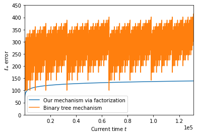
Figure 1: Additive $\ell_{\infty}$ error with $T=2^{16},\epsilon=0.8,\delta=10^{-10}$.

Our contributions. We prove concrete bounds on the additive error for counting under continual release that is tight up to a small additive gap. Since our bounds are closed-form expressions, it is straightforward to evaluate them for any data analysis task. Furthermore, our algorithms only perform few matrix-vector multiplications and additions, which makes them easy to implement and tailor to operations natively implemented in modern hardware. Finally, our algorithms are also efficient and the additive error of the output is smooth. As counting is a versatile building block, we get concrete bounds on a wide class of problems under continual release such as maintaining histograms, generating synthetic graphs that preserve cut sizes, computing various graph functions, and substring and counting episode in string sequences (see Section 1.2 for more details). Furthermore, this also leads to an improvement in the additive error for non-interactive local learning [STU17], private learning on non-Euclidean geometry [AFKT21], and private online prediction [AFKT22]: These algorithms use the binary mechanism as a subroutine and using our mechanism instead would give a constant-factor improvements in the additive error. This in turn allows to decrease the privacy parameter in private learning, which is highly desirable and listed as motivation in several recent works [AFT22, DMR⁺22, HUU23].

Our bounds bridge the gap between theoretical work on differential privacy, which mostly concentrates on asymptotic analysis to reveal the capabilities of differential private algorithms, and practical applications, which need to obtain useful information from differential private algorithms for their specific use cases.

Organization. The rest of this section gives the formal problem statement, an overview of results, technical contribution, and comparison with related works. Section 2 gives the necessary definitions, Section 3 presents the formal proof of our main result, Section 5 contains all its applications we explored. We give lower bounds in Section 6 and present experiments in Section 7.

1.1 The Formal Problem

Linear queries are classically defined as follows: There is a universe ${\cal X}=\{0,1\}^{d}$ of values and a set ${\mathcal{Q}}=\{q_{1},\dots,q_{k}\}$ of functions $q_{i}:{\cal X}\rightarrow\mathbb{R}$ with $1\leqslant i\leqslant k$. Given a vector $x=(x[1],\dots,x[n])$ of $n$ values of $\cal X$ (with repetitions allowed) a linear query $q(x)$ for the function $q$ computes $\sum_{j=1}^{n}q(x[j])$. A workload for a vector $x$ and a set $\{q_{1},\dots,q_{k}\}$ of functions computes the linear query $q_{i}(x)$ for each function $q_{i}$ with $1\leqslant i\leqslant k$. This computation can be formalized using linear algebra notation as follows: Assume there is a fixed ordering $y_{1},\dots y_{2^{d}}$ of all elements of $\cal X$. The workload matrix $M$ is defined by $M[i,j]=q_{i}(y_{j})$, i.e. there is a row for each function $q_{i}$ and a column for each value $y_{j}$. Let $h\in\mathbb{N}_{0}^{2^{d}}$ be the histogram vector of $x$, i.e. $y_{j}$ appears $h(y_{j})$ times in $x$. Then answering the linear queries is equivalent to computing $Mh$.

In the continual release setting, the vector $x$ is given incrementally to the mechanism in rounds or time steps. In time step $t$, $x[t]$ is revealed to the mechanism and it has to output $M_{t}x$ under differential privacy, where $M$ is the workload matrix and $M_{t}$ denotes the $t\times t$ principal submatrix of $M$.

Binary counting corresponds to a very simple linear query in this setting: The universe ${\cal X}$ equals $\{0,1\}$, there is only one query $q:{\cal X}\rightarrow\mathbb{R}$ with $q(1)=1$ and $q(0)=0$. However, alternatively, binary counting could also be expressed as follows and this is the notation that we will use: There is only one query $q^{\prime}$ with $q^{\prime}(y)=1$ for all $y\in{\cal X}$ giving rise to a simple workload matrix $M=(1,\dots,1)$ for the static setting and the mechanism outputs $Mx$. Thus, in the continual release setting, we study the following the following workload matrix, $M_{\mathsf{count}}\in\{0,1\}^{T\times T}$:

$$M_{\mathsf{count}}[i,j]=\begin{cases}1&i\geqslant j\\ 0&i<j\end{cases}$$ (1)

where for any matrix $A$, $A[i,j]$ denote its $(i,j)$^th coordinate.

There has been a large body of work on designing differentially private algorithms for general workload matrices in the static setting, i.e., not under continual release. One of the scalable techniques that provably reduces the error on linear queries is a query matrix optimization technique known as workload optimizer (see [MMHM21] and references therein). There have been various algorithms developed for this, one of them being the matrix mechanism [LMH⁺15], which first determines two matrices $R$ and $L$ such that $M=LR$ and then outputs $L(Rx+z)$, where $z\sim N(0,\sigma^{2}\mathbb{I})$ is a vector of Gaussian values for a suitable choice of $\sigma^{2}$ and $\mathbb{I}$ is the identity matrix. For a privacy budget $(\epsilon,\delta)$, it can be shown that the additive error, denoted as $\ell_{\infty}$ error of the answer vector (see Definition 3), of the matrix mechanism for $|\mathcal{Q}|$ linear queries with $\ell_{2}$-sensitivity $\Delta_{\mathcal{Q}}$ (eq. 7) represented by a workload matrix $M$ using the Gaussian mechanism is as follows: with probability $2/3$ over the random coins of the algorithm, the additive error is at most

$$\underbrace{\frac{2}{\epsilon}\sqrt{{\frac{4}{9}+\ln\left({\frac{1}{\delta}\sqrt{\frac{2}{\pi}}}\right)}}}_{C_{\epsilon,\delta}}\Delta_{\mathcal{Q}}\left\|L\right\|_{2\to\infty}\left\|R\right\|_{1\to 2}\sqrt{\ln(6|\mathcal{Q}|)},\vspace{-5mm}$$ (2)

where $\left\|A\right\|_{2\to\infty}$ (resp., $\left\|A\right\|_{1\to 2}$) is the maximum $\ell_{2}$ norm of rows (resp. columns) of $A$. The function $C_{\epsilon,\delta}$ is a function arising as in the proof of the privacy guarantee of the Gaussian mechanism when $\epsilon<1$ (see Theorem A.1 in [DR14]. If $\epsilon\geqslant 1$, one can analytically compute $C_{\epsilon,\delta}$ using Algorithm 1 in [BW18]. For the rest of this paper, we use $C_{\epsilon,\delta}$ to denote this function. Therefore, we need to find a factorization $M=LR$ that minimizes $\left\|L\right\|_{2\to\infty}\left\|R\right\|_{1\to 2}$. Note that the quantity

$$\left\|M\right\|_{\mathsf{cb}} =\min_{M=LR}\left\{{\left\|L\right\|_{2\to\infty}\left\|R\right\|_{1\to 2}}\right\}=\max_{W}{\frac{\left\|W\bullet M\right\|}{\left\|W\right\|}}.$$

is the completely bounded norm (abbreviated as cb-norm). Here ${W\bullet M}$ denotes the Schur product [Sch11].

The factor $C_{\epsilon,\delta}\Delta_{\mathcal{Q}}\sqrt{\ln(6|\mathcal{Q}|}$ in equation (2) is due to the error bound of the Gaussian mechanism followed by the union bound and is the same for all factorizations. Thus to get a concrete additive error, we need to find a factorization $M=LR$ such that the quantity $\left\|M\right\|_{\mathsf{cb}}$ is not just small, but also can be computed concretely. Furthermore we observe that if both $L$ and $R$ are lower-triangular matrices, then the resulting mechanism works not only in the static setting, but also in the continual release model. Therefore, for the rest of the paper, we only focus on finding such a factorization of the workload matrix $M_{\mathsf{count}}$, which is a fundamental query in the continual release model.

1.2 Our Results

1. Bounding $\left\|M_{\mathsf{count}}\right\|_{\mathsf{cb}}$. The question of finding the optimal value of $\left\|M_{\mathsf{count}}\right\|_{\mathsf{cb}}$ was also raised in the conference version of [MNT20], who showed asymptotically tight bound. In the past, there has been considerable effort to get a tight bound on $\left\|M_{\mathsf{count}}\right\|_{\mathsf{cb}}$ [Dav84, Mat93] with the best-known result is the following due to Mathias [Mat93, Corollary 3.5]:

$$\begin{split}\left({\frac{1}{2}+\frac{1}{2T}}\right)\widehat{\gamma}(T)\leqslant\left\|M_{\mathsf{count}}\right\|_{\mathsf{cb}}\leqslant\frac{\widehat{\gamma}(T)}{2}+\frac{1}{2},\end{split}$$ (3)

$\text{where}~{}\widehat{\gamma}(T)=\frac{1}{T}\sum_{j=1}^{T}\left|{\csc\left({\frac{(2j-1)\pi}{2T}}\right)}\right|.$

The key point to note is that the proof of [Mat93] relies on the dual characterization of cb-norm, and, thus, does not give an explicit factorization. In contrast, we give an explicit factorization into lower triangular matrices that achieve a bound in terms of the function, $\Psi:\mathbb{N}\to\mathbb{R}$ defined over natural numbers as follows:

$$\Psi(T):=1+{1\over\pi}\left({\ln\left(\dfrac{4T-3}{5}\right)}\right).$$ (4)

Theorem 1 (Upper bound on $\left\|M_{\mathsf{count}}\right\|_{\mathsf{cb}}$).

Let $M_{\mathsf{count}}\in\left\{{0,1}\right\}^{T\times T}$ be the matrix defined in eq. 1. Then, there is an explicit factorization $M_{\mathsf{count}}=LR$ into lower triangular matrices such that

$$\left\|L\right\|_{2\to\infty}\left\|R\right\|_{1\to 2}\leqslant\Psi(T).$$ (5)

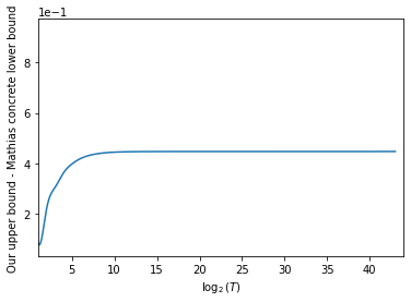
Figure 2: Difference between our upper bound and the explicitly computed Mathias lower bound.

The bounds in eq. 3 do not have a closed form formula; however, we can show that it converges in limit as $T\to\infty$ (Lemma 6). However, our focus in this paper is on concrete bounds and exact factorization. Our (theoretical) upper bound and the (analytically computed) lower bound of [Mat93] are less than $0.5$ apart for all $2^{5}\leqslant T\leqslant 2^{44}$ (Figure 2).

Additionally, our result has the advantage that we achieve the bound with an explicit factorization of $M_{\mathsf{count}}=LR$ such that both $L$ and $R$ are lower-triangular matrices. As discussed above, this allows us to use it for various applications. Using this fact and carefully choosing the “noise vector” for every time epoch, the following result is a consequence of Theorem 1 and eq. 2:

Theorem 2 (Upper bound on differentially private continual counting).

Let $\epsilon,\delta\in(0,1)$ be the privacy parameters. There is an $(\epsilon,\delta)$-differentially private algorithm for binary counting in the continual release model with output $a_{t}$ in round $t$ such that in every execution, with probability at least $1-\beta$ over the coin tosses of the algorithm, simultaneously, for all rounds $t$ with $1\leq t\leq T$, it holds that

$$\left|a_{t}-\sum_{i=1}^{t}x_{i}\right|\leqslant C_{\epsilon,\delta}\Psi(t)\sqrt{2\ln(T/\beta)},$$ (6)

where $\Psi(t)$ is as in eq. 4. The time to output $a_{t}$ in round $t$ is $O(t)$.

As mentioned above, the binary mechanism of [CSS11] and [DNPR10] and its improvement (when the error metric is expected mean squared) by [Hon15] can be seen as factorization mechanism. This has been independently noticed by [DMR⁺22]. While [CSS11] and [DNPR10] do work in the continual release model, [Hon15]’s optimization does not because for a partial sum, $\sum_{i\leqslant t}x_{i}$, it also uses the information stored at the nodes formed after time $t$. Therefore, for the comparison with related work, we do not include Honaker’s optimization [Hon15]. Moreover, Honaker’s optimization is for minimizing the expected mean squared error (i.e., in $\ell_{2}^{2}$ norm), and not the $\ell_{\infty}$ error, which is the focus of our work. To the best of our knowledge, only [CSS11] and [DNPR10] consider additive error in terms of $\ell_{\infty}$ norm. All other approaches used for binary counting under continual observation (see [WCZ⁺21] and references therein) use some form of smoothening of the output and consider the expected mean squared error. While useful in some applications, many applications require to bound the additive $\ell_{\infty}$ error.

The most relevant work to ours is the subsequent work by [HUU23] that show that our factorization gives almost tight concrete bounds on performing counting under continual observation with respect to the expected mean squared error. On the other hand, we bound the maximum absolute additive error, i.e., in $\ell_{\infty}$ norm of the error. Note that our explicit factorization for $M_{\mathsf{count}}$ has the nice property that there are exactly $T$ distinct entries (instead of possibly $T^{2}$ entries in [DMR⁺22])’s factorization. This has a large impact on computation time.

Remark 1 (Suboptimality of the binary mechanism with respect to the constant).

The binary mechanism computes a linear combination of the entries in the streamed vector $x$ as all of the internal nodes of the binary tree can be seen as a linear combinations of the entries of $x$. Now we can consider the binary mechanism as a matrix mechanism. The right factor $R_{\mathsf{binary}}$ is constructed as follows: $R_{\mathsf{binary}}=W_{m}$ where $W_{1},\cdots,W_{m}$ are defined recursively as follows:

$$W_{1}=\begin{pmatrix}1\end{pmatrix},\quad W_{k}=\begin{pmatrix}W_{k-1}&0\\ 0&W_{k-1}\\ 1_{2^{k-2}}&1_{2^{k-2}}\end{pmatrix},\quad k\leqslant m.$$

That is, $R_{\mathsf{binary}}=W_{m}\in\left\{{0,1}\right\}^{(2T-1)\times T}$, with each row corresponding to the partial sum computed for the corresponding node in the binary tree from leaf $i$ to the root. The corresponding matrix $L_{\mathsf{binary}}$ is a matrix in $\left\{{0,1}\right\}^{T\times(2T-1)}$, where row $i$ has a one in at most $\log_{2}(i)$ entries, corresponding exactly to the binary representation of $i$.

In particular, this factorization view tells us that $\left\|L\right\|_{2\to\infty}\left\|R\right\|_{1\to 2}={\log_{2}(T)}{(\log_{2}(T)+1)}$, which implies that the $\ell_{\infty}$-error is suboptimal by a factor of $\pi\log_{2}(e)$. Our experiments (Figure 3) confirm this behavior experimentally. With respect to the mean-squared error this was observed by several works [DMR⁺22, Hon15] culminating in the work of [HUU23], who gave a theoretical proof for the suboptimality of binary mechanism for mean-squared error.

Applications.

Our result for continual binary counting can be extended in various directions. We show how to use it to quantify the additive error for (1) outputting a synthetic graph on the same vertex set which approximately preserves the values of all $(S,P)$-cuts with $S$ and $P$ being disjoint vertex sets of the graph, (2) frequency estimation (aka histogram estimation), (3) various graph functions, (4) substring counting, and (5) episode counting. Our mechanism can also be adapted for the locally private non-interactive learners of [STU17] by replacing the binary mechanism with our matrix mechanism, which requires major changes in the analysis. In Table 1, we tabulate these applications. Based on a lower bound construction of [JRSS21], we show in Section 6 that for large enough $T$ and constant $|S|$ the additive error in (1) is tight up to polylogarithmic factors and the additive error in (4) is tight for large enough $T$ up to a factor that is linear in $\log\log|{\mathcal{U}|}\ln T$, where $\mathcal{U}$ is the universe of letters (see Corollary 4 and Section 6 for details). Finally, we can use our mechanism to estimate the running average of a sequence of $T$ bits with absolute error $\Psi(t)C_{\epsilon,\delta}\sqrt{\ln(6T)}/t$. All the applications are presented in detail in Section 5. We note that all our algorithms are differentially private in the setting considered in [DNPR10].

Table 1: Applications of Theorem 1 ($\epsilon,\delta\in(0,1)$ are privacy parameter, $\eta\in(0,1)$ is the multiplicative approximation parameter, $u$ is the dimension of each data item for histogram estimation and $b$ a bound on its $\ell_{0}$-sensitivity, and $U$ is the set of letters, $\ell$ is the maximum length of the substrings that are counted, $T$ is the length of the stream), $n$ is the number of users in local-DP. Here, graph functions include subgraph counting, cost of minimum spanning tree, etc.

Problem	Additive error	Reference
$(S,P)$-cuts (with $|S|\leqslant|T|$)	$3C_{\epsilon,\delta}|S|\Psi(T)\sqrt{(|S|+|P|)\ln(|S|+|P|)\ln(6T)}$	Corollary 1
Histogram estimation	$C_{\epsilon,\delta}\Psi(T)\sqrt{b\ln(6\lvert U\rvert T)}$	Corollary 2
Graph functions	$C_{\epsilon,\delta}{\Psi(T)\sqrt{\ln(6T)}}$	Corollary 3
Counting all length $\leq\ell$ substrings	$C_{\epsilon,\delta}\Psi(T)\ell\sqrt{\ln(6T\lvert U\rvert^{\ell})}$	Corollary 4
Counting all length $\leq\ell$ episodes	$2C_{\epsilon,\delta}\Psi(T)\ell\sqrt{\lvert U\rvert^{\ell-1}\ell\ln(6T\lvert U\rvert^{\ell})}$	Corollary 5
$1$-dimensional local convex risk min.	$C_{\frac{\epsilon}{2},\frac{\delta}{2}}\sqrt{\frac{\ln(6(\epsilon\sqrt{n}+1))}{2n}}\left({1+\frac{\ln((4\epsilon\sqrt{n}-3))/5}{\pi}}\right)+\frac{2}{\epsilon\sqrt{n}}$	Corollary 6

2. Lower Bounds. We now turn our attention to new lower bounds on continual counting under approximate differential privacy. Prior to this paper, the only known lower bound for differentially private continual observation was for counting under pure differential privacy. There are a few other methods to prove lower bounds. For example, we can use the relation between hereditary discrepancy and private linear queries [MN12] along with the generic lower bound on hereditary discrepancy [MNT20] to get an $\Omega(1)$ lower bound. This can be improved by using the reduction of continual counting to the threshold and get an $\Omega(\log^{*}(T))$ [BNSV15].

Our lower bound is for a class of mechanisms, called data-independent mechanisms, that add a random variable sampled from the distribution which is independent of the input. Most commonly used differentially private mechanisms, such as the Laplace mechanism and the Gaussian mechanism fall under this class.

For binary counting, recall from eq. 3 that there exists a lower bound on $\left\|M_{\mathsf{count}}\right\|_{\mathsf{cb}}$ in terms of $\widehat{\gamma}(T)$. In Lemma 6, we show that

$$\lim_{T\to\infty}\widehat{\gamma}(T)\to\frac{2\ln(T)}{\pi}$$

from above. Combined with the proof idea of [ENU20], this gives the following bound for non-adaptive input streams, i.e., where the input stream is generated before seeing any output of the mechanism.

Theorem 3 (Lower bound).

Let $\epsilon,\delta$ be a sufficiently small constant and $\mathfrak{M}$ be the set of data-independent $(\epsilon,\delta)$-differentially private algorithms for binary counting under non-adaptive continual observation. Then

$$\max_{x\in\left\{{0,1}\right\}^{T}}\mathbb{E}_{\mathcal{M}\in\mathfrak{M}}\left[{\left\|\mathcal{M}(x)-M_{\mathsf{count}}x\right\|_{\infty}^{2}}\right]\in\Omega\left({\frac{\ln^{2}(T)}{\epsilon^{2}}}\right).$$

That is, the variance of the $\ell_{\infty}$-error is $\Omega(\ln^{2}(T)/\epsilon^{2})$. A formal proof of Theorem 3 is presented in Section 6.

1.3 Our Technical Contribution

1. Using the matrix mechanism in the continual release model. Our idea to use the matrix mechanism ${\cal F}$ in the continual release model is as follows: Assume $M$ is known to ${\cal F}$ before any items of the stream $x$ arrive and there exists an explicit factorization of $M=LR$ into lower triangular matrices $L$ and $R$ that can be computed efficiently by ${\cal F}$ during preprocessing. As we show, this is the case for the matrix $M_{\mathsf{count}}$. This property leads to the following mechanism: At time $t$, the mechanism ${\cal F}$ creates $x^{\prime}$ with consists of the current $x$-vector with $T-t$ zeros appended, and then returns the $t$^th entry of $L(Rx^{\prime}+z)$, where $z$ is a suitable “noise vector”. As $L$ and $R$ are lower-triangular, the $t$^th entry of $L(Rx^{\prime}+z)$ is identical to the $t$^th entry in $L(Rx^{f}+z)$, where $x^{f}$ is the final input vector $x$, and, thus, it suffices to analyze the error of the static matrix mechanism. Note that our algorithm can be implemented so that it requires time $O(t)$ at time $t$. The advantage of this approach is that it allows us to use the analysis of the static matrix mechanism while getting an explicit bound on the additive error of the mechanism in the continual release model.

Factorization in terms of lower triangular matrices is not known to be necessary for the continual release model; however, [DMR⁺22] pointed out that an arbitrary factorization will not work. For example, they discuss that [Hon15]’s optimization of the binary mechanism can be seen as a factorization but it cannot be used for continual release as the output of his linear program at time $t$ can give positive weights to values of $x$ generated at a future time $t^{\prime}>t$. Furthermore, as instead of computing $L(Rx^{\prime}+z)$ we work with $t\times t$-dimensional submatrices of $L$ and $R$, we can replace a $\log T$ factor in the upper bound on the additive error due to the binary mechanism by a $\ln(t)$, where $t\leqslant T$ denotes the current time step.

2. Bounding $\left\|M_{\mathsf{count}}\right\|_{\mathsf{cb}}$. The upper bound can be derived in various ways. One direct approach would be to find appropriate Kraus operators of a linear map and then use the characterization by [HP93] of completely bounded norm. This approach yields an upper bound of $1+\frac{\ln(T)}{\pi}$; however, it does not directly give lower triangular factorization $L$ and $R$.

Instead we use the characterization given by [Pau82], which gives us a factorization in terms of lower triangular matrices. More precisely, using three basic trigonometric identities, we show that the $(i,j)$^th entry of $R$ and $L$ is an integral of every even power of the cosine function, $\frac{2}{\pi}\int\limits_{0}^{\pi/2}\cos^{2(i-j)}(\theta)\mathsf{d}\theta$ for $i\geqslant j$. This choice of matrices leads to the upper bound in eq. 5.

3. Applications. While counting and averaging under continual release follows from bounds in Theorem 1, computing cut-functions requires some ingenuity. In particular, one can consider $(S,P)$-cuts for an $n$-vertex graph $\mathcal{G}=(V,E,w)$ as linear queries by constructing a matrix $M$ whose rows correspond to each possible cut query $(S,P)\in V\times V$ and whose columns corresponds to all possible edges in $\mathcal{G}$. The entry $((S,P),j)$ of $M$ equals to $1$ if the edge $j$ crosses the boundary of the cut $(S,P)$. However, it is not clear how to use it in the matrix mechanism efficiently because known algorithm for finding a factorization as well as the resulting factorization depend polynomial on the dimension of the matrix and the number of rows in $M$ is $O(2^{n})$. Instead we show how to exploit the algebraic structure of cut functions so that at each time step $t$ the mechanism only has to compute $L_{t}R(t)x(t)$, where $L_{t}$ is a ${n\choose 2}\times t{n\choose 2}$-dimensional matrix, $R(t)$ is $t{n\choose 2}\times t{n\choose 2}$-dimensional matrix and $x(t)$ is $t{n\choose 2}$-dimensional. This gives an mechanism that has error $O(\min(|S|,|P|)\ln(t)\sqrt{(|S|+|P|)\ln(|S|+|P|)\ln(6T)}$ (see Corollary 1 for exact constant) and can be implemented to run in time $O(tn^{4})$ per time step.

Binary counting can also be extended to histogram estimation. [CR21] gave a differentially private mechanism for histogram estimation where in each time epoch exactly one item either arrives or is removed. We extend our approach to work in the setting that they call known-domain, restricted $\ell_{0}$-sensitivity and improve the constant factor in the additive error by the same amount as for binary counting.

We also show in Section 5.6 an application of our mechanism to non-interactive local learning. The non-interactive algorithm for local convex risk minimization is an adaption of the algorithm of [STU17], which uses the binary tree mechanism for binary counting as a subroutine. Replacing it by our mechanism for binary counting (Theorem 2) leads to various technical challenges: From the algorithmic design perspective, [STU17] used the binary mechanism with a randomization routine from [DJW13], which expects as input a binary vector, while we apply randomization to $Rx$, where $R$ has real-valued entries. We overcome this difficulty by using two instead of one binary counter. From an analysis point of view, the error analysis in [STU17] is based on the error analysis in [BS15] that uses various techniques, such as the randomizer of [DJW13], error-correcting codes, and the Johnson-Lindenstrauss lemma. However, one can show that we can give the same uniform approximation (see Definition 5 in [STU17] for the formal definition) as in [STU17] by using the Gaussian mechanism and two binary counters so that the rest of their analysis applies.

2 Notations and Preliminaries

We use $v[i]$ to denote the $i$^th coordinate of a vector $v$. For a matrix $A$, we use $A[i,j]$ to denote its $(i,j)$^th coordinate, $A[:,i]$ to denote its $i$^th column, $A[i,:]$ to denote its $i$^th row, $\left\|A\right\|_{\mathsf{tr}}$ to denote its trace norm of square matrix, $\|A\|_{F}$ to denote its Frobenius norm, $\left\|A\right\|$ to denote its operator norm, and $A^{\top}$ to denote transpose of $A$. We use $\mathbb{I}_{d}$ to denote identity matrix of dimension $d$. If all the eigenvalues of a symmetrix matrix $S\in\mathbb{R}^{d\times d}$ are non-negative, then the matrix is known as positive semidefinite (PSD for short) and is denoted by $S\succeq 0$. For symmetric matrices $A,B\in\mathbb{R}^{d\times d}$, the notations $A\preceq B$ implies that $B-A$ is PSD. For an $a_{1}\times a_{2}$ matrix $A$, its tensor product (or Kronecker product) with another matrix $B$ is

$$\begin{pmatrix}A[1,1]B&A[1,2]B&\cdots&A[1,a_{2}]B\\ A[2,1]B&A[2,2]B&\cdots&A[2,a_{2}]B\\ \vdots&\ddots&\vdots\\ A[a_{1},1]B&A[a_{1},2]B&\cdots&A[a_{1},a_{2}]B\\ \end{pmatrix}.$$

We use $A\otimes B$ to denote the tensor product of $A$ and $B$. In our case, the matrix $B$ would always be identity matrix of appropriate dimension.

One main application of our results is in differential privacy formally defined below:

Definition 1.

A randomized mechanism $\mathcal{M}$ gives $(\epsilon,\delta)$-differential privacy if for all neighboring data sets $D$ and $D^{\prime}$ in the domain of $\mathcal{M}$ differing in at most one row, and all measurable subset $S$ in the range of $\mathcal{M}$, $\mathsf{Pr}\left[{\mathcal{M}(D)\in S}\right]\leqslant e^{-\varepsilon}\mathsf{Pr}\left[{\mathcal{M}(D^{\prime})\in S}\right]+\delta,$ where the probability is over the private coins of $\mathcal{M}$.

This definition requires, however, to define neighboring data sets in the continual release model. In this model the data is given as a stream of individual data items, each belonging to a unique user, each arriving one after the other, one per time step. In the privacy literature, there are two well-studied notions of neighboring streams [CSS11, DNPR10]: (i) user-level privacy, where two streams are neighboring if they differ in potentially all data items of a single user; and (ii) event-level privacy, where two streams are neighboring if they differ in a single data item in the stream. We here study event-level privacy.

Our algorithm uses the Gaussian mechanism. To define the Gaussian mechanism, we need to first define $\ell_{2}$-sensitivity. For a function $f:\mathcal{X}^{n}\to\mathbb{R}^{d}$ its $\ell_{2}$-sensitivity is defined as

$$\Delta f:=\max_{\text{neighboring }X,X^{\prime}\in\mathcal{X}^{n}}\left\|f(X)-f(X^{\prime})\right\|_{2}.$$ (7)

Definition 2 (Gaussian mechanism).

Let $f:\mathcal{X}^{n}\to\mathbb{R}^{d}$ be a function with $\ell_{2}$-sensitivity $\Delta f$. For a given $\epsilon,\delta\in(0,1)$ the Gaussian mechanism $\mathcal{M}$, which given $X\in\mathcal{X}^{n}$ returns $\mathcal{M}(X)=f(X)+e$, where $e\sim\mathcal{N}(0,C_{\epsilon,\delta}^{2}(\Delta f)^{2}\mathbb{I}_{d})$, satisfies $(\epsilon,\delta)$-differential privacy.

Definition 3 (Accuracy).

A mechanism ${\cal M}$ is $(\alpha,T)$-accurate for a function $f$ if, for all finite input streams $x$ of length $T$, the maximum absolute error satisfies $||f(x)-{\cal M}(x)||_{\infty}\leqslant\alpha$ with probability at least $2/3$ over the coins of the mechanism.

3 Proof of Theorem 1

The proof of Theorem 1 relies on the following lemmas.

Lemma 1 ([CQ05]).

For integer $m$, define $\mathcal{S}_{m}:=\left({\frac{1}{2}}\right)\left({\frac{3}{4}}\right)\cdots\left({\frac{2m-1}{2m}}\right).$ Then, $\mathcal{S}_{m}\leqslant\sqrt{\frac{1}{\pi(m+1/4)}}.$

Proof of Theorem 1.

Define a function, $f:\mathbb{Z}_{+}\to\mathbb{R}$, recursively as follows

$$f(0)=1~{}\text{and}~{}f(k)=\left({\frac{2k-1}{2k}}\right)f(k-1);\;k\geqslant 1.$$ (8)

Since the function $f$ satisfies a nice recurrence relation, it is very easy to compute. Let $L$ and $R$ be defined as follows:

$$R[i,j]=L[i,j]=f(i-j).$$ (9)

Lemma 2.

Let $M_{\mathsf{count}}\in\left\{{0,1}\right\}^{T\times T}$ be the matrix defined in eq. 1. Then $M_{\mathsf{count}}=LR$.

Proof.

One way to prove the lemma is by using trigonometric inequalities for $\cos(2\theta)$ and that (i) For any $\theta\in[-\pi,\pi]$, $\sin^{2}(\theta)+\cos^{2}(\theta)=1$, (ii) For even $m$, $\frac{2}{\pi}\int\limits_{0}^{\pi/2}\cos^{m}(\theta)\mathsf{d}\theta=\left({\frac{1}{2}}\right)\left({\frac{3}{4}}\right)\cdots\left({\frac{m-1}{m}}\right)$, (iii) For all $\theta\in[-\pi,\pi]$, $\cos(2\theta)=2\cos^{2}(\theta)-1.$ This proof would require a lot of algebraic manipulations. However, our proof relies on an observation that all the three matrices, $L,R,$ and $M_{\mathsf{count}}$ are $T\times T$ principal submatrix of Toeplitz operators. The main idea would be to represent Toeplitz operator in its functional form: Let $a_{1},a_{2},\cdots,\in\mathbb{C}$ denote the entries of the Toeplitz operator, $\mathcal{T}$, with complex entries. Then its unique associated symbol is

$$f_{\mathcal{T}}(z)=\sum_{n=0}^{\infty}a_{n}z^{n},$$

where $z\in\mathbb{C}$ such that $|z|=1$. We can then write $z=e^{\iota\theta}$ for $0\leqslant\theta\leqslant 2\pi$. Then for operator ${\mathcal{M}}$ whose principal $T\times T$ submatrix is the matrix $M_{\mathsf{count}}$, we arrive that its associated symbol is

$$f_{\mathcal{M}}(\theta)=\sum_{n=0}^{\infty}e^{\iota\theta n}=\left({1-e^{\iota\theta}}\right)^{-1}.$$

Let $\mathcal{L}$ denote the Toeplitz operator whose $T\times T$ submatrix is the matrix $L$ and $\mathcal{R}$ denote the Toeplitz operator whose $T\times T$ submatrix is the matrix $R$. Then the symbol associated with $\mathcal{L}$ and $\mathcal{R}$ is

$$f_{{\mathcal{R}}}(\theta)=f_{{\mathcal{L}}}(\theta) =\sum_{n=0}^{\infty}f(n)e^{\iota\theta n}=1+\frac{1}{2}e^{\iota\theta}+\frac{3}{8}e^{2\iota\theta}+\cdots$$ (10)

Now $(1-x)^{-1/2}=1+\frac{1}{2}x+\frac{3}{8}x^{2}+\cdots$. Therefore, comparing the terms, we can rewrite eq. 10 as follows:

$$f_{{\mathcal{L}}}(\theta)=\left({1-e^{\iota\theta}}\right)^{-1/2}\quad\text{and}\quad f_{{\mathcal{R}}}(\theta)=\left({1-e^{\iota\theta}}\right)^{-1/2}.$$

Since, for any two Toeplitz operators, $\mathcal{A}$ and $\mathcal{B}$ with associated symbols $f_{\mathcal{A}}(\theta)$ and $f_{\mathcal{B}}(\theta)$, respectively, $\mathcal{A}\mathcal{B}$ has the associated symbol $f_{\mathcal{A}}(\theta)f_{\mathcal{B}}(\theta)$ [BG00], we have the lemma. ∎

Using Lemma 1, we have

$$\left\|L\right\|_{2\to\infty}^{2} =\sum_{i=0}^{T-1}f(i)^{2}=1+\sum_{i=1}^{T-1}f(i)^{2}$$

$$\leqslant 1+{1\over\pi}\sum_{i=1}^{T-1}{1\over i+1/4}$$

$$\leqslant 1+{1\over\pi}\int\limits_{i=1}^{T-1}{1\over i+1/4}$$

$$\leqslant 1+{1\over\pi}\left({\ln\left(\dfrac{4T-3}{5}\right)}\right)$$

Combining with the fact that $\left\|L\right\|_{2\to\infty}=\left\|L\right\|_{1\to 2}$ and $R=L$, we have the following:

Lemma 3.

Let $L$ and $R$ be $T\times T$ matrices defined by eq. 9. Then $\left\|L\right\|_{1\to 2}=\left\|L\right\|_{2\to\infty}=\left\|R\right\|_{1\to 2}=\left\|R\right\|_{2\to\infty}$. Further,

$$\left\|L\right\|_{2\to\infty}^{2}\leqslant 1+{1\over\pi}\left({\ln\left(\dfrac{4T-3}{5}\right)}\right).$$

Theorem 1 follows from Lemma 2 and 3. ∎

4 Proof of Theorem 2

Fix a time $t\leqslant T$. Let $L_{t}$ denote the $t\times t$ principal submatrix of $L$ and $R_{t}$ be the $t\times t$ principal submatrix of $R$. Let the vector formed by the streamed bits be $x_{t}=\begin{pmatrix}x[1]&\cdots&x[t]\end{pmatrix}\in\left\{{0,1}\right\}^{t}$. Let $z_{t}=\begin{pmatrix}z[1]&\cdots&z[t]\end{pmatrix}$ be a freshly sampled Gaussian vector such that $z[i]\sim\mathcal{N}(0,C_{\epsilon,\delta}^{2}\left\|R_{t}\right\|_{1\to 2}^{2})$.

Let $M_{\mathsf{count}}(t)$ denote the $t\times t$ principal submatrix of $M_{\mathsf{count}}$. The algorithm computes

$$\widetilde{x}_{t}=L_{t}(R_{t}x_{t}+z_{t}) =L_{t}R_{t}x_{t}+L_{t}z_{t}=M_{\mathsf{count}}(t)x_{t}+L_{t}z_{t}$$

and outputs the $t$^th coordinate of $\widetilde{x}_{t}$ (denoted by $x_{t}[t]$). So far, the data structure maintained by the mechanism when it enters round $t$ is simply $x_{t-1}$. Now, note that the $t$^th coordinate of $M_{\mathsf{count}}(t)x_{t}$ equals the sum of the first $t$ bits and can be computed in constant time when the sum of the bits of the previous round $t-1$ is known (i.e., maintained). Then, sampling a fresh Gaussian vector $z_{t}$ and computing the $t$^th coordinate of $L_{t}z_{t}$ takes time $O(t)$. For privacy, note that the $\ell_{2}$-sensitivity of $R_{t}x_{t}$ is $\left\|R_{t}\right\|_{1\to 2}$; therefore, adding Gaussian noise with variance $\sigma_{t}^{2}=C_{\epsilon,\delta}^{2}\left\|R_{t}\right\|_{1\to 2}^{2}$ preserves $(\epsilon,\delta)$-differential privacy. Now for the accuracy guarantee,

$$\widetilde{x}_{t}[t]=\sum_{i=1}^{t}x[i]+\sum_{i=1}^{t}L_{t}[t,i]z_{t}[i].$$

Therefore,

$$\left|\widetilde{x}_{t}[t]-\sum_{i=1}^{t}x[i]\right|=\left|\sum_{i=1}^{t}L_{t}[t,i]z_{t}[i]\right|.$$

Recall that $z[i]\sim\mathcal{N}(0,\sigma_{t}^{2})$. The Cauchy-Schwarz inequality shows that the function $\ell(z_{t}):=\sum_{i=1}^{t}L_{t}[t,i]z[i]$ has Lipschitz constant $\left\|L_{t}\right\|_{2\to\infty}$, i.e., the maximum row norm. Now define $z^{\prime}[i]:=z[i]/\sigma_{t}$ and note that $z^{\prime}[i]\sim\mathcal{N}(0,1)$ and $\mathbb{E}[\ell(z_{t}^{\prime})]=\mathbb{E}[\ell(z_{t})]=0$. Using the concentration inequality for Gaussian random variables with unit variance and a function $f$ with Lipschitz constant $\left\|L_{t}\right\|_{2\to\infty}$ (e.g., Proposition 4 in [Zei16]) implies that

$$\mathsf{Pr}_{z_{t}}\left[{\left|\ell(z_{t})-\mathbb{E}[\ell(z_{t})]\right|>a}\right]$$

$$=\mathsf{Pr}_{z_{t}}\left[{\left|\ell(z_{t}^{\prime})-\mathbb{E}[\ell(z_{t}^{\prime})]\right|>a/\sigma_{t}}\right]\leqslant 2e^{-a^{2}/(2\sigma^{2}_{t}\left\|L_{t}\right\|_{2\to\infty}^{2})}.$$

Setting

$$a=\sqrt{2}\sigma_{t}\left\|L_{t}\right\|_{2\to\infty}\log(2T/\beta)=\sqrt{2}C_{\epsilon,\delta}\left\|R_{t}\right\|_{1\to 2}\left\|L_{t}\right\|_{2\to\infty}\log(2T/\beta),$$

the result follows using a union bound over all $T$ time steps and Theorem 1, which implies that $\left\|L_{t}\right\|_{2\to\infty}=\left\|R_{t}\right\|_{1\to 2}\leq\sqrt{\Psi(t)}$.

5 Applications in Continual Release

5.1 Continuously releasing a synthetic graph which approximates all cuts.

For a weighted graph $\mathcal{G}=(V,E,w)$, we let $n$ denote the size of the vertex set $V$ and $m$ denote the size of the edge set $E$. When the graph is uniformly weighted (i.e., all existing edges have the same weight, all non-existing have weight 0), then the graph is denoted $\mathcal{G}=(V,E)$. Let $W$ be a diagonal matrix with non-negative edge weights on the diagonal. If we define an orientation of the edges of graph, then we can define the signed edge-vertex incidence matrix $A_{\mathcal{G}}\in\mathbb{R}^{m\times n}$ as follows:

$$A_{\mathcal{G}}[e,v]=\left\{\begin{array}[]{rl}1&\text{if }v\text{ is }e\text{'s head},\\ -1&\text{if }v\text{ is }e\text{'s tail},\\ 0&\text{otherwise}.\end{array}\right.$$

One important matrix representation of a graph is its Laplacian (or Kirchhoff matrix). For a graph $\mathcal{G}$, its Laplacian $K_{\mathcal{G}}$ is the matrix form of the negative discrete Laplace operator on a graph that approximates the negative continuous Laplacian obtained by the finite difference method.

Definition 4 ($(S,P)$-cut).

For two disjoint subsets $S$ and $P$, the size of the cut $(S,P)$-cut is denoted $\Phi_{S,P}(\mathcal{G})$ and defined as

$$\Phi_{S,P}(\mathcal{G}):=\sum_{u\in S,v\in P}w\left({u,v}\right).$$

When $P=V\backslash S$, we denote $\Phi_{S,P}(\mathcal{G})$ by $\Phi_{S}(\mathcal{G})$.

In this section we study the following problem. Let $\mathcal{G}=(V,E,w)$ be a weighted graph and consider a sequence of $T$ updates to the edges of $\mathcal{G}$, where each update consists of an (edge,weight) tuple with weight in $[0,1]$ that adds the weight to the corresponding edge. For $t$, $1\leqslant t\leqslant T$, let $\mathcal{G}_{t}$ denote the graph that is obtained by applying the first $t$ updates to $\mathcal{G}$. We give a differentially private mechanism that returns after each update $t$ a graph $\overline{\mathcal{G}}_{t}$ such that for every cut $(S,P)$ with $S\cap P=\emptyset$, the number of edges crossing the cut in $\overline{\mathcal{G}}_{t}$ differs from the number of edges crossing the same cut in $\mathcal{G}_{t}$ by at most $O(\min\{|S|,|P|\}\sqrt{n\ln n}\ln^{3/2}T)$:

Corollary 1.

There is an $(\epsilon,\delta)$-differentially private algorithm that, for any stream of edge updates of length $T>0$, outputs a synthetic graph $\overline{\mathcal{G}}_{t}$ in round $t$ and with probability at least 2/3 over the coin tosses of the algorithm, simultaneously for all rounds $t$ with $1\leq t\leq T$, it holds that for any $S,P\subset V$ with $S\cap P=\emptyset$,

$$\Phi_{S,P}(\overline{\mathcal{G}}_{t}) \leqslant\Phi_{S,P}(\mathcal{G}_{t})+3C_{\epsilon,\delta}|S|\psi(t)\sqrt{(|S|+|P|)\ln(|S|+|P|)\ln(6T)},$$

where $\mathcal{G}_{t}$ is the graph formed at time $t$ through edge updates and $C_{\epsilon,\delta}$ is as defined in eq. 2. The time for round $t$ is $O(tn^{4})$.

Proof.

Let us first analyze the case where $P=V\setminus S$. In this case, we encode the updates as an $\mathbb{R}^{n\choose 2}$ vector and consider the following counting matrix:

$$M_{\mathsf{cut}}=M_{\mathsf{count}}\otimes\mathbb{I}_{n\choose 2}\in\left\{{0,1}\right\}^{T{n\choose 2}\times T{n\choose 2}}$$

For the rest of this subsection, we drop the subscript and denote $\mathbb{I}_{n\choose 2}$ by $\mathbb{I}$. Recall the function $f$ defined by eq. 8. Let $L_{\mathsf{count}}[i,j]=f(i-j)$. Using this function, we can compute the following factorization of $M_{\mathsf{cut}}$: $L=L_{\mathsf{count}}\otimes\mathbb{I}\text{ and }R=L.$ Let $R(t)$ and $L(t)$ denote the $t{n\choose 2}\times t{n\choose 2}$ principal submatrix of $R$ and $L$, respectively. They both consist of $t$ block matrices, each being formed by all columns and $n\choose 2$ rows of $R$ and $L$, respectively. Further, let $R_{t}$ and $L_{t}$ denote the $t$^th block matrix of $n\choose 2$ rows of $R$ and $L$, respectively. Let $x(t)$ be the $t\times{n\choose 2}$ vector formed by the first $t$ updates, i.e., the edges of $\mathcal{G}_{t}$ which are given by the ${n\choose 2}$ vector $E_{\mathcal{G}_{t}}:=L_{t}R(t)x(t).$

Let $C_{\epsilon,\delta}$ be the function of $\epsilon$ and $\delta$ stated in eq. 6 and $\sigma^{2}=C_{\epsilon,\delta}^{2}\left\|R_{t}\right\|_{1\to 2}^{2}\sqrt{\ln(6T)}$. Then the edges of the weighted graph $\overline{\mathcal{G}}_{t}$ which is output at time $t$ are given by the ${n\choose 2}$ vector $L_{t}\left(R(t)x(t)+z\right),$ where $z\sim\mathcal{N}(0,\sigma^{2})^{t\times{n\choose 2}}$. Note that computing the output naively takes time $O(t^{2}n^{4})$ to compute $R(t)x(t)$, time $O(tn^{2})$ to generate and add $z$, and time $O(tn^{4})$ to multiply the result with $L_{t}$. However, if we store the vector of $R(t-1)x(t-1)$ of the previous round and only compute $R_{t}x(t)$ in round $t$, then the vector $R(t)x(t)$ can be created by “appending” $R_{t}x(t)$ to the vector $R(t-1)x(t-1)$. Thus, $R(t)x(t)$ can be computed in time $O(tn^{4})$, which reduces the total computation time at time step $t$ to $O(tn^{4})$.

We next analyse the additive error of this mechanism. The output at time $t$ of the algorithm is a vector indicating the edges as $E_{\overline{\mathcal{G}}_{t}}=L_{t}(R(t)x(t)+z)=E_{\mathcal{G}_{t}}+L_{t}z.$ Let $f_{t}=\begin{pmatrix}f(t-1)&\cdots&f(0)\end{pmatrix}^{\top}\in\mathbb{R}^{t}$ be a row vector whose coordinates are the evaluations of the function $f(\cdot)$ on $\left\{{0,1,\cdots,t-1}\right\}$. Then $L_{t}=f_{t}\otimes\mathbb{I}$.

As $L_{t}z$ is the weighted sum of random variables from $N(0,\sigma^{2})$, it holds that $L_{t}z\sim N(0,\left\|L_{t}\right\|^{2}_{2\to\infty}\sigma^{2}{\mathbb{I}}_{n\choose 2}).$ In other words, the error is due to a graph, $\mathcal{R}$, with weights sampled from a Gaussian distribution $N(0,C_{\epsilon,\delta}^{2}\left\|L_{t}\right\|^{2}_{2\to\infty}\left\|R(t)\right\|_{1\to 2}^{2}{\mathbb{I}})$.

For a subset $S\subseteq[n]$, let

$$\chi_{S}=\sum_{i\in S}\overline{e}_{i},$$

where $\overline{e}_{i}$ is the $i$^th standard basis. It is known that for any positive weighted graph ${\mathcal{G}}$, the $(S,V\backslash S)$-cut $\Phi_{S}(\mathcal{G})=\chi_{S}^{\top}K_{\mathcal{G}}\chi_{S}$. So, for any subset $S\subseteq[n]$, $|\Phi_{S}(\overline{\mathcal{G}}_{t})-\Phi_{S}(\mathcal{G}_{t})|\leqslant\sqrt{\Psi(t)}\left|\chi_{S}^{\top}K_{\mathcal{R}}\chi_{S}\right|.$

The proof now follows on the same line as in Upadhyay et al. [UUA21]. In more details, if $K_{n}$ denotes the Laplacian of the complete graph with $n$ vertices, then $K_{\mathcal{R}}\preceq 3\sigma\sqrt{\frac{\ln(n)}{n}}{K_{n}}$. Here, $A\preceq B$ means that $x^{\top}(B-A)x\geqslant 0$ for all $x$. Setting $\sigma=3C_{\epsilon,\delta}\Psi(t)\sqrt{\ln(6T)}$, the union bound gives that with probability at least $2/3$, simultaneously for all rounds $T$,

$$\left|\chi_{S}^{\top}K_{\mathcal{R}}\chi_{S}\right| \leqslant 3\sigma\sqrt{\frac{\ln(n)}{n}}\left|\chi_{S}^{\top}{L_{n}}\chi_{S}\right|={3\sigma|S|\left(n-|S|\right)}\sqrt{\frac{\ln(n)}{n}}$$

$$\leqslant 3\sigma\sqrt{n\ln(n)}|S|=3C_{\epsilon,\delta}|S|\Psi(t)\sqrt{n\ln(n)\ln(6T)}.$$ (11)

We next consider the case of $(S,P)$ cuts, where $S\cup P\subseteq V$ and $S\cap P=\emptyset$. Without loss of generality, let $|S|\leqslant|P|$. Let us denote by $\mathcal{G}_{A}$ the graph induced by a vertex set $A\subseteq V$. In this case, for the analysis, we can consider the subgraph, $\mathcal{G}_{S\cup P}$, formed by the vertex set $S\cup P$. By Fiedler’s result [Fie73], $s_{i}(\mathcal{G}_{S\cup P})\leqslant s_{i}(\mathcal{G}_{V})$, where $s_{i}(\mathcal{H})$ denotes the $i$^th singular value of the Laplacian of the graph $\mathcal{H}$. Considering this subgraph, we have reduced the analysis of $(S,P)$ cut on $\mathcal{G}$ to the analysis of $(S,\overline{S})$-cut on $\mathcal{G}_{S\cup P}$. Therefore, using the previous analysis, we get the result.

We now give the privacy proof. At time $t$, we only need to prove privacy for $R(t)x(t)+z$ as multiplication by $L_{t}$ can be seen as post-processing. Now consider two neighboring graphs form by the stream of (edge, weight) tuple, where at time $\tau$, they differ in weight. If $t<\tau$, the output distribution is the same because the input is the same. So, consider $t\geqslant\tau$. At this point, $x(t)$ and $x^{\prime}(t)$ differ in exactly $t-\tau$ positions by at most $1$. Breaking $x(t)-x^{\prime}(t)$ in blocks of $n\choose 2$ coordinates, the position where $x(t)-x^{\prime}(t)$ is $1$ is exactly corresponding to the edge they differ. Now multiplying with $R(t)$ results in vector whose non-zero entries are $\left\{{f(\tau),\cdots,f(t)}\right\}$. Using Lemma 3, $\left\|R(t)(x(t)-x^{\prime}(t))\right\|_{2}^{2}=\left\|R_{t}\right\|_{2}^{2}-\left\|R_{\tau}\right\|_{2}^{2}\leqslant\left\|R_{t}\right\|_{2}^{2}$. Therefore, we have $(\epsilon,\delta)$-differential privacy from the choice of $\sigma$ and Definition 2. ∎

Remark 2.

In the worst case when $|S|=cn$ for some constant $c>0$, this results in an additive error of order $n^{3/2}\sqrt{\ln n}\ln^{3/2}T$. This result gives a mechanism for maintaining the minimum cut as well as a mechanism for maintaining the maximum cut, sparsest cuts, etc with such an additive error. Moreover, we can extend the result to receive updates with weights in $[-1,1]$ as long as the underlying graph only has positive weights at all time.

For maintaining the minimum cut in the continual release model we show in Appendix 6 that our upper bound is tight up to polylogarithmic factors in $n$ and $T$ for large enough $T$ and constant $S$ using a reduction from a lower bound in [JRSS21].

Our mechanism can implement a mechanism for the static setting as it allows to insert all edges of the static graph in one time step. The additive error that we achieve can even be a slight improvement over the additive error of $O(\sqrt{nm/\epsilon}\ln^{2}(n/\delta))$, where $m$ is the sum of the edge weights, achieved by the mechanism in [EKKL20]. Note also that our bound does not contradict the lower bound for the additive error in that paper, as they show a lower bound only for the case that $\max\{|S|,|P|\}=\Omega(n)$.

5.2 Continual histogram

Continual histogram. Modifying the analysis for cut functions, we can use our algorithm to compute the histogram of each column for a data base of $u$-dimensional binary vectors in the continual release model in a very straightforward manner. Said differently, assume $\mathcal{U}$ is a universe of size $u$ and the input at a time step consists of the indicator vector of a subset of $\mathcal{U}$, which is a $u$-dimensional binary vector. Let $b$ with $1\leq b\leq u$ be the maximum number of 1s in the vector, i.e., the maximum size of a subset given at a time step.

Corollary 2.

Let $\mathcal{U}$ be the universe of size $u$ and let $1\leq b\leq u$ be a given integer. Consider a stream of $T$ vectors $x_{t}\in\left\{{0,1}\right\}^{u}$ such that $x_{t}[j]=1$ if $j\in\mathcal{S}$ and $x_{t}[k]=0$ for all $k\not\in\mathcal{S}$ where at time $t$ the subset ${\mathcal{S}}\subseteq{\mathcal{U}}$ with $|{\mathcal{S}}|\leq b$ is streamed. Then there is an efficient $(\epsilon,\delta)$-differentially private algorithm which outputs a vector $h_{t}\in\mathbb{R}^{u}$ in round $t$ such that, with probability at least 2/3 over the coin tosses of the algorithm, simultaneously, for all rounds $t$ with $1\leq t\leq T$, it holds that

$$\left\|h_{t}-\sum_{i=1}^{t}x_{i}\right\|_{\infty}\leqslant C_{\epsilon,\delta}\Psi(t)\sqrt{b\ln(6uT)}.$$

The same bounds hold if items can also be removed, i.e., $x_{t}\in\left\{{-1,0,1}\right\}^{u}$ as long as $\sum_{i=1}^{t}x_{i}[j]\geq 0$ for all $1\leqslant j\leqslant u$ and all $t\leqslant T$.

Proof.

We consider the following matrix: $M_{\mathsf{hist}}=M_{\mathsf{count}}\otimes\mathbb{I}_{u}$ with every update being the indicator vector in $\left\{{0,1}\right\}^{u}$. We drop the subscript on $\mathbb{I}$ and denote $\mathbb{I}_{u}$ by $\mathbb{I}$ in the remainder of this subsection. Recall the function $f$ defined by eq. 8. Let $L_{\mathsf{count}}[i,j]=f(i-j)$. Using this function, we can compute the following factorization of $M_{\mathsf{hist}}$: $L=L_{\mathsf{count}}\otimes\mathbb{I}\text{ and }R=L.$ Let $R(t)$, resp. $L(t)$, be the $tu\times tu$ principal submatrix of $R$, resp. $L$. Let $R_{t}$, resp. $L_{t}$, be the $t$^th block matrix of $R(t)$, resp. $L(t)$, consisting of all columns and the last $u$ rows. Then at any time epoch we output $h_{t}=L_{t}(R(t)x(t)+z_{t})$, where $x(t)\in\left\{{0,1}\right\}^{tu}$ is the row-wise stacking of $x_{1},\cdots,x_{t}$ and $z_{t}[i]\sim N(0,\sigma^{2}_{t})$ for $\sigma^{2}_{t}=C_{\epsilon,\delta}^{2}b\left\|R_{t}\right\|_{1\to 2}^{2}$. For privacy, note that the $\ell_{2}$-sensitivity of $R_{t}x_{t}$ is $\sqrt{b}\left\|R_{t}\right\|_{1\to 2}$; therefore, adding Gaussian noise with variance $\sigma_{t}^{2}=C_{\epsilon,\delta}^{2}b\left\|R_{t}\right\|_{1\to 2}^{2}$ preserves $(\epsilon,\delta)$-differential privacy.

Using the same proof as in the case of $M_{\mathsf{count}}$ we obtain

$$\left\|h_{t}-\sum_{i=1}^{t}x_{i}\right\|_{\infty}\leqslant C_{\epsilon,\delta}\left\|R_{T}\right\|_{1\to 2}\left\|L_{T}\right\|_{2\to\infty}\sqrt{b\ln(6uT)}.$$

Using Theorem 1, we have the corollary. ∎

5.3 Other graph functions

Our upper bounds can also be applied to continual release algorithms that use the binary mechanism to compute prefix sums. Let $f_{1},f_{2},\dots,f_{T}$ be a sequence $\sigma$ of $T$ function values. The difference sequence of $\sigma$ is $f_{2}-f_{1},f_{3}-f_{2},\dots,f_{T}-f_{T-1}$. For a graph function under continual release, its sensitivity may depend on the allowed types of edge updates. [FHO21] show that the $\ell_{1}$-sensitivity of the difference sequence of the cost of a minimum spanning tree, degree histograms, triangle count and $k$-star count does not depend on $T$ for partially dynamic updates (either edge insertions or deletions) and is $\Omega(T)$ for fully dynamic updates (edge insertions and/or deletions). Using this result, they prove that one can privately compute these graph functions under continual observation by releasing noisy partial sums of the difference sequences of the respective functions. More generally, they show the following result for any graph function with bounded sensitivity of the difference sequence.

Lemma 4 ([FHO21], cf Corollary 13).

Let $f$ be a graph function whose difference sequence has $\ell_{1}$-sensitivity $\Gamma$. Let $0<p<1$ and $\varepsilon>0$. For each $T\in\mathbb{N}$, the binary mechanism yields an $\epsilon$-differentially private algorithm to estimate $f$ on a graph sequence, which has additive error $O(\Gamma\varepsilon^{-1}\cdot\ln^{3/2}T\cdot\ln p^{-1})$ with probability at least $1-p$.

We replace the summation by the binary mechanism in Lemma 4 by summation using $M_{\mathsf{count}}$, getting the following result.

Corollary 3.

Let $f$ be a graph function whose difference sequence has $\ell_{2}$-sensitivity $\Gamma$. There is an $(\epsilon,\delta)$-differentially private algorithm that, for any sequence of edge updates of length $T>0$ to a graph $\mathcal{G}$, with probability at least 2/3 over the coin tosses of the algorithm, simultaneously for all rounds $t$ with $1\leq t\leq T$, outputs at time $t$ an estimate of $f(\mathcal{G}_{t})$ that has additive error at most $C_{\epsilon,\delta}\Psi(t)\Gamma\sqrt{\ln(6T)}$.

5.4 Counting Substrings

We can also extend our mechanism for counting all substrings of length at most $\ell$, where $\ell\geqslant 1$, in a sequence $\sigma$ of letters. After each update $i$ (i.e., a letter), we consider the binary vector $v_{\sigma,i}$ that is indexed by all substrings of length at most $\ell$. The value of $v_{\sigma,i}[s]$, which corresponds to the substring $s$, indicates whether the suffix of length $\lvert s\rvert$ of the current sequence equals $s$. We can cast the problem of counting substrings as a binary sum problem on the sequence of vectors $v_{\sigma,\cdot}$ and apply $M_{\mathsf{ep}}=M_{\mathsf{count}}\otimes\mathbb{I}_{u}$ to the concatenated vectors, where $u={\sum_{i\leqslant\ell}\lvert\mathcal{U}\rvert^{i}}$.

Corollary 4.

Let $\mathcal{U}$ be a universe of letters, let $\ell\geqslant 1$. There exists an $(\epsilon,\delta)$-differentially private algorithm that, given a sequence of letters $s=s_{1}\cdots s_{T}$ from $\mathcal{U}$, outputs, after each letter, the approximate numbers of substrings of length at most $\ell$. With probability at least 2/3 over the coin tosses of the algorithm, simultaneously, for all rounds $t$ with $1\leq t\leq T$, the algorithm has at time $t$ an additive error of at most $C_{\epsilon,\delta}\Psi(t)\ell\sqrt{\ln(2\lvert U\rvert^{\ell})\ln(6T)}$, where $C_{\epsilon,\delta}$ is as defined in eq. 2.

Proof.

Let $\sigma=\sigma_{1}\cdots\sigma_{T}$ and $\sigma^{\prime}=\sigma^{\prime}_{1}\cdots\sigma^{\prime}_{T}$ be two sequences of letters that differ in only one position $p$, i.e., $\sigma_{i}=\sigma^{\prime}_{i}$ if and only if $i\neq p$. We observe that $v_{\sigma,i}=v_{\sigma^{\prime},i}$ for any $i\notin\{p,\ldots,p+\ell-1\}$. Furthermore, for any $i$, $0\leqslant i<\ell$ and $j$, $i+1\leqslant j\leqslant\ell$, there exist only two substrings $s$ of length $j$ so that $v_{\sigma,p+i}[s]\neq v_{\sigma^{\prime},p+i}[s]$. It follows that the $\ell_{2}$-sensitivity is at most $\sqrt{\sum_{i=0}^{\ell-1}\sum_{j=i+1}^{\ell}2}\leqslant\sqrt{\ell^{2}}=\ell$. Using $\sum_{i\leqslant\ell}\lvert\mathcal{U}\rvert^{i}\leqslant 2\lvert U\lvert^{\ell}$, the proof concludes analogously to the proof of Corollary 2. ∎

5.5 Episodes

Given a universe of events (or letters) $\mathcal{U}$, an episode $e$ of length $\ell$ is a word over the alphabet $\mathcal{U}$, i.e., $e=e_{1}\cdots e_{\ell}$ so that for each $i$, $1\leqslant i\leqslant\ell$, $e_{i}\in\mathcal{U}$. Given a string $s=s_{1}\cdots s_{n}\in\mathcal{U}^{*}$, an occurence of $e$ in $s$ is a subsequence of $s$ that equals $e$. A minimal occurrence of an epsiode $e$ in $s$ is a subsequence of $s$ that equals $e$ and whose corresponding substring of $s$ does not contain another subsequence that equals $e$. In other words, $s_{i_{1}}\cdots s_{i_{\ell}}$ is a minimal occurence of $e$ in $s$ if and only if (1) for all $j$, $1\leqslant j\leqslant\ell$, $s_{i_{j}}=e_{j}$ and (2) there does not exist $s_{j_{1}}\cdots s_{j_{\ell}}$ so that for all $k$, $1\leqslant k\leqslant\ell$, $s_{j_{k}}=e_{k}$, and either $i_{1}<j_{1}$ and $j_{\ell}\leqslant i_{\ell}$, or $i_{1}\leqslant j_{1}$ and $j_{\ell}<i_{\ell}$. The support of an episode $e$ on a string $s$ is the number of characters from the string that are part of at least one minimal occurrence of $e$. Note that for an episode $e$, its minimal occurrences may overlap. For the non-differentially private setting, Lin et al. [LQW14] provide an algorithm that dynamically maintains the number of minimal occurrences of episodes in a stream of events. For better performance, the counts may be restricted to those episodes that have some minimum support on the input (i.e., frequent episodes).

Lemma 5 ([LQW14]).

Let $\mathcal{U}$ be a universe of events, let $\ell\geqslant 2$, and let $S\geq 1$. There exists a (non-private) algorithm that, given a sequence of events $s=s_{1}\cdots s_{T}$ from $\mathcal{U}$, outputs, after each event, the number of minimal occurrences for each episode of length at most $\ell$ that has support at least $S$. The time complexity per update is $\tilde{O}(T/S+\lvert\mathcal{U}\rvert^{2})$ and the space complexity of the algorithm is $\tilde{O}(\lvert U\rvert\cdot T/S+\lvert\mathcal{U}\rvert^{2}\cdot T)$.

There can be at most one minimal occurrence of $e$ that ends at a fixed element $s_{t}\in s$. Therefore, we can view the output of the algorithm after event $s_{t}$ as a binary vector $v_{t}\in\{0,1\}^{\sum_{i\leqslant\ell}\lvert\mathcal{U}\rvert^{i}}$ that is indexed by all episodes of length at most $\ell$ and that indicates, after each event $s_{t}$, if a minimal occurrences of epsiode $e$ ends at $s_{t}$. Summing up the (binary) entries corresponding to $e$ in $v_{1},\ldots,v_{t}$ yields the number of minimal occurrences of $e$ in $s_{1}\cdots s_{t}$. Therefore, we can cast this problem of counting minimal occurrences of episodes as a binary sum problem and apply $M_{\mathsf{ep}}$.

Corollary 5.

Let $\mathcal{U}$ be a universe of events, let $\ell\geqslant 2$, and let $S\geq 1$. There exists an $(\epsilon,\delta)$-differentially private mechanism that, given a sequence of events $s=s_{1}\cdots s_{T}$ from $\mathcal{U}$, outputs, after each event, the approximate number of minimal occurrences for each episode of length at most $\ell$ that has support at least $S$. With probability at least 2/3 over the coin tosses of the algorithm, simultaneously for all rounds $t$ with $1\leq t\leq T$ the algorithm has at time $t$ an additive error of at most $C_{\epsilon,\delta}\Psi(t)\sqrt{\lvert U\rvert^{\ell-1}\ell\ln(2\lvert U\rvert^{\ell})\ln(6T)}$.

Proof.

Let $\sigma=\sigma_{1}\cdots\sigma_{T}$ and $\sigma^{\prime}=\sigma^{\prime}_{1}\cdots\sigma^{\prime}_{T}$ be two sequences of letters that differ in only one position $p$, i.e., $\sigma_{i}=\sigma^{\prime}_{i}$ if and only if $i\neq p$. Recall that we are only interested in minimal occurences of episodes. Therefore, the number of query answers that are different for $\sigma$ and $\sigma^{\prime}$ are trivially upper bounded by two times the maximum number of episodes that end on the same character (once for $\sigma[p]$ and once for $\sigma^{\prime}[p]$), times the maximum length of an episode (as for every episode that ends at $p$, only the one with the latest start is a minimal occurrence). This is bounded by $2\sum_{i\leqslant\ell}\lvert\mathcal{U}\rvert^{i-1}\cdot\ell\leqslant 4\lvert U\rvert^{\ell-1}\ell$. It follows that the global $\ell_{2}$-sensitivity is at most $2\sqrt{\lvert U\rvert^{\ell-1}\ell}$. Using $\sum_{i\leqslant\ell}\lvert\mathcal{U}\rvert^{i}\leqslant 2\lvert U\lvert^{\ell}$, the proof concludes analogously to the proof of Corollary 2. ∎

On sparse streams. Until now, we have focused mainly on worst case analysis. We next consider the case when the stream is sparse, i.e., number of ones in the stream is upper bounded by a parameter $s$. Dwork et al. [DNRR15] showed that under this assumption, one can asymtotically improve the error bound on continual release to $O\left({\frac{\log(T)+\log^{2}(s)}{\epsilon}}\right)$ while preserving $\epsilon$-differential privacy. Using their analysis combined with our bounds we directly get the error bound $C_{\epsilon,\delta}\left({5\log(T)+\Psi(n)\sqrt{\ln(6n)}}\right).$

5.6 Non-interactive Local Learning

In this section, we consider convex risk minimization in the non-interactive local differential privacy mode (LDP) using Theorem 1. That is, there are $n$ participants (also known as clients) and one server. Every client has a private input $d_{i}$ from a fixed universe $\mathcal{D}$. To retain the privacy of this input, each client applies a differentially-private mechanism to their data (local model) and then sends a single message to the server which allows the server to perform the desired computation (convex risk minimization in our case). After receiving all messages, the server outputs the result without further interaction with the clients (non-interactive).

In $1$-dimensional convex risk minimization, a problem is specified by a convex, closed and bounded constraint set $\mathcal{C}$ in $\mathbb{R}$ and a function $\ell:\mathcal{C}\times\mathcal{D}\to\mathbb{R}$ which is convex in its first argument, that is, for all $D\in\mathcal{D}$, $\ell(\cdot;D)$ is convex. A data set $D=(d_{1},\ldots,d_{n})\in\mathcal{D}^{n}$ defines a loss (or empirical risk) function: $\mathcal{L}(\theta;D)=\tfrac{1}{n}\sum_{i=1}^{n}\ell(\theta;d_{i})$, where $\theta$ is a variable that is chosen as to minimize the loss function. The goal of the algorithm is to output a function $f$ that assigns to each input $D$ a value $\theta\in\mathcal{C}$ that minimizes the average loss over the data sample $D$. For example, finding the median of the 1-dimensional data set $D\in[0,1]^{n}$ consisting of $n$ points in the interval $[0,1]$ corresponds to finding $\theta\in\mathcal{C}$ that minimizes the loss $\mathcal{L}(\theta,D)=\sum_{i}|\theta-d_{i}|$.

When the inputs are drawn i.i.d. from an underlying distribution $\mathcal{P}$ over the data universe $\mathcal{D}$, one can also seek to minimize the population risk: $\mathcal{L}_{\mathcal{P}}(\theta)=\mathsf{E}_{D\sim\mathcal{P}}[\ell(\theta;D)].$ We will use some notations in this section. Let $I_{1},\cdots,I_{w}$ be $w$ disjoint intervals of $[0,1]$ of size $s:=\lfloor{\frac{1}{\epsilon\sqrt{n}}}\rfloor$. Let $\mathcal{B}=\left\{{j\cdot s:0\leqslant j\leqslant w}\right\}$. Given a vector $a\in\mathbb{R}^{w}$ let $g$ be a “continuous intrapolation” of the vector $a$, namely $g:[0,1]^{w}\times[0,1]\to[0,1]$ such that $g(a,\theta)=a[k]$, where $k=\operatornamewithlimits{argmin}_{z\in\mathcal{B}}|z-\theta|$, with ties broken for smaller values. Also, let $f:\mathbb{R}^{w}\times[0,1]\to[0,1]$ be defined as $f(a,x)=\int\limits_{0}^{x}g(a,t)\mathsf{d}t$.

[STU17] showed the following:

Theorem 4 (Corollary 8 in [STU17]).

For every 1-Lipschitz loss function $\ell:[0,1]\times\mathcal{D}\to\mathbb{R}$, there is a randomized algorithm $Z:\mathcal{D}\to[0,1]$, such that for every distribution $\mathcal{P}$ on $\mathcal{D}$, the distribution $\mathcal{Q}$ on $[0,1]$ obtained by running $Z$ on a single draw from $\mathcal{P}$ satisfies $\mathcal{L}_{\mathcal{P}}(\theta)=\mathsf{med}_{\mathcal{Q}}(\theta)$ for all $\theta\in[0,1]$, where $\mathsf{med}_{\mathcal{P}}(\theta)={\mathbb{E}}_{d\sim\mathcal{Q}}[|\theta-d|]$.

In other words, differentially private small error for 1-dimensional median is enough to solve differentially private loss minimization for general $1$-Lipschitz functions. Prior work used a binary mechanism to determine the 1-dimensional median. We show how to replace this mechanism by the factorization mechanism of Theorem 2. As the reduction in Theorem 4 preserves exactly the additive error, our analysis of the additive error in Theorem 2 carries through, giving a concrete upper bound on the additive error.

We first recall the algorithm of [STU17]. Median is non-differentiable at its minimizer $\theta^{*}$, but in any open interval around $\theta^{*}$, its gradient is either $+1$ or $-1$. $\mathsf{STU}$ first divides the interval $[0,1]$ into $w=\lceil{\epsilon\sqrt{n}}\rceil$ disjoint intervals $I_{1},\cdots,I_{w}$ of $[0,1]$ of size $s:=\lfloor{\frac{1}{\epsilon\sqrt{n}}}\rfloor$. Let $\mathcal{B}=\left\{{j\cdot s:0\leqslant j\leqslant w}\right\}$. Every client constructs a $w$-dimensional binary vector that has $1$ only on the coordinate $j$ if its data point $d_{i}\in I_{j}$. The client then executes the binary mechanism with the randomizer of Duchi et al. [DJW13] on its vector and sends the binary tree to the server. Based on this information the server computes a vector $x^{\mathsf{STU}}\in\mathbb{R}^{w}$, where $x^{\mathsf{STU}}[j]$ is the $1/n$ times the difference of the number of points in the interval $\cup_{l=1}^{j}I_{l}$ and the number of data points in the interval $\cup_{l=j+1}^{w}I_{l}$. The server outputs the function $f(x^{\mathsf{STU}},\theta)$.

To replace the binary tree mechanism used in [STU17] (dubbed as $\mathsf{STU}$) into a factorization mechanism based algorithm is not straightforward because of two reasons: (i) Smith et al. used the binary mechanism with a randomization routine from [DJW13], which expects as input a binary vector, while we apply randomization to $Rx$, where $x$ is the binary vector, and (ii) the error analysis is based on the error analysis in [BS15] which does not carry over to the factorization mechanism.

We now describe how we modify $\mathsf{STU}$ to give an LDP algorithm $\mathcal{A}$. Instead of forming a binary tree, every client $i$ forms two binary vectors $u_{i},v_{i}\in\left\{{0,1}\right\}^{w}$ with $u_{i}[j]=v_{i}[w-j]=1$ if $d_{i}\in I_{j}$ and 0 otherwise. Note that in both vectors exactly 1 bit is set and that

$$\left(\sum_{i=1}^{n}\sum_{l=1}^{t}u_{i}[l]\right)-\left(\sum_{i=1}^{n}\sum_{l=t+1}^{w}v_{i}[l]\right)$$

gives the number of bits in the interval $\cup_{l=1}^{t}I_{l}$ minus the number of data points in the interval $\cup_{l=t+1}^{w}I_{l}$. The user now sends two vectors $y_{i},z_{i}\in\mathbb{R}^{w}$ to the server formed by running the binary counter mechanism defined in Theorem 2 on $u_{i}$ and $v_{i}$ with privacy parameters $(\frac{\epsilon}{2},\frac{\delta}{2})$. Since the client’s message is computed using a differentially private mechanism for each vector, the resulting distributed mechanism is $(\epsilon,\delta)$-LDP using the basic composition theorem.

On receiving these vectors, the server first computes the aggregate vector

$$\widehat{x}[t]=\frac{1}{n}\left(\sum_{i=1}^{n}y_{i}[t]-\sum_{i=1}^{n}z_{i}[w-t]\right).$$ (12)

The server then computes and outputs $f(\widehat{x},\theta)$.

To analyze our mechanism let $x^{\mathsf{STU}}$ be the vector formed in $\mathsf{STU}$ and $\widetilde{x}$ be the vector that the server in $\mathsf{STU}$ would have formed if clients did not use any randomizer. Equation (3) in [STU17] first showed that, for all

$$\begin{split}\forall\theta\in[0,1],\quad\left|g(x^{\mathsf{STU}},\theta)-g(\widetilde{x},\theta)\right|\leqslant\alpha\quad\\ \text{for}\quad\alpha\in O\left({\frac{\log^{2}(\varepsilon^{2}n)\sqrt{\log(\varepsilon^{2}n)}}{\varepsilon\sqrt{n}}}\right).\end{split}$$ (13)

[STU17] (see Theorem 6) then use the fact that $f(x,\theta)=\int\limits_{0}^{\theta}g(x;s)\mathsf{d}s$ to show that $\left|f(x^{\mathsf{STU}},\theta)-\mathsf{med}_{\mathcal{P}}(\theta)\right|\leqslant\left|g(x^{\mathsf{STU}},\theta)-g(\widetilde{x},\theta)\right|+\frac{2}{\epsilon{\sqrt{n}}}$ and use eq. 13 to get their final bound, which is $O\left({\frac{\log^{2}(\varepsilon^{2}n)\sqrt{\log(\varepsilon^{2}n)}}{\varepsilon\sqrt{n}}}\right)$. We remark that we can replace $x^{\mathsf{STU}}$ by any $y\in\mathbb{R}^{w}$ as long as $\left|g(y,\theta)-g(\widetilde{x},\theta)\right|\leqslant\alpha$ for all $\theta\in[0,1]$.

We now show an equivalent result to eq. 13. We argue that the vector $\widehat{x}$ serves the same purpose as $x^{\mathsf{STU}}$. The key observation here is that $\sum_{i=1}^{n}y_{i}[t]$ contains the partial sum for the intervals $I_{1},\dots,I_{t}$ and $\sum_{i=1}^{n}z_{i}[w-t]$ contains the partial sum for $I_{j+1},\dots,I_{w}$. Let $\overline{x}=\frac{1}{n}(\sum_{i=1}^{n}u_{i}[t]-\sum_{i=1}^{n}v_{i}[w-t])$ be the vector corresponding to the estimates in eq. 12 if no privacy mechanism was used. Note that $\widetilde{x}=\overline{x}$. Since the randomness used by different clients is independent,

$$\mathsf{Var}[\widehat{x}[t]]=\frac{1}{{n^{2}}}\mathsf{Var}\left[{\sum_{i=1}^{n}(y_{i}[t]-z_{i}[w-t])}\right]$$

$$=\frac{2}{n^{2}}\mathsf{Var}\left[{\sum_{i=1}^{n}y_{i}[t]}\right]=\frac{2}{n^{2}}\sum_{i=1}^{n}\mathsf{Var}\left[{y_{i}[t]}\right]=\frac{2}{n}\sigma_{t},$$

where $\sigma_{t}$ is the variance used in the binary counting mechanism of Theorem 2. Using the concentration bound as in the proof of Theorem 2, we have $\left\|\widehat{x}-\overline{x}\right\|_{\infty}\leqslant 2\beta$ with $\beta=C_{\frac{\epsilon}{2},\frac{\delta}{2}}\sqrt{\frac{\ln(6(\epsilon\sqrt{n}+1))}{2n}}\left({1+\frac{\ln((4\epsilon\sqrt{n}-3))/5}{\pi}}\right)$. By the definition of $g(\cdot,\cdot)$, we therefore have $\forall\theta\in[0,1]$, $\left|g(\widehat{x},\theta)-g(\overline{x},\theta)\right|\leqslant 2\beta.$

Now using the same line of argument as in [STU17], we get the following bound:

Corollary 6.

For every distribution $\mathcal{P}$ on $[0,1]$, with probability $2/3$ over $D\sim\mathcal{P}^{n}$ and $\mathcal{A}$, the output $\widehat{f}\leftarrow\mathcal{A}$ satisfies $\left|f(\widehat{x},\theta)-\mathsf{med}_{\mathcal{P}}(\theta)\right|\leqslant 2\beta+\frac{2}{\epsilon\sqrt{n}}$, where $\mathsf{med}_{\mathcal{P}}(\theta)={\mathbb{E}}_{d\sim\mathcal{Q}}[|\theta-d|]$. Further, $\mathcal{A}$ is $(\epsilon,\delta)$-LDP.

Our algorithm $\mathcal{A}$ is non-interactive $(\epsilon,\delta)$-LDP algorithm and not $\epsilon$-LDP as $\mathsf{STU}$, but we can give $\mathcal{A}$ our algorithm as input to the GenProt transformation (Algorithm 3) in [BNS19] to turn it into a $(10\epsilon,0)$-LDP algorithm (see Lemma 6.2 in [BNS19]) at the cost of increasing the population risk using Theorem 6.1 in [BNS19].

6 Lower bounds

Definition 5 (Max-Cut).

Given a graph $\mathcal{G}=(V,E,w)$, the maximum cut of the graph is the optimization problem

$$\max_{S\subseteq V}\left\{\Phi_{S}(\mathcal{G})\right\}=\max_{S\subseteq V}\left\{\sum_{u\in S,v\in V\backslash S}w\left({u,v}\right)\right\}.$$

Let $\mathsf{OPT}_{\mathsf{max}}(\mathcal{G})$ denote the maximum value.

In this section we use a reduction from the maximum sum problem. Let ${\cal X}=\{0,1\}^{d}$, let $x\in{\cal X}^{T}$, $d\in\mathbb{N}$, and for $1\leqslant j\leqslant d$, let $x_{t}[j]$ denote the $j$-th coordinate of record $x_{t}$. A mechanism for the $d$-dimensional maximum sum problem under continual observation is to return for each $0\leqslant t\leqslant T$, the value $\max_{1\leqslant j\leqslant d}\sum_{s=1}^{t}x_{s}[j]$.

In [JRSS21] Jain et al. studied the problem of computing in the continual release model the maximum sum of a $d$-dimensional vector. Two vectors $x$ and $x^{\prime}$ are neighboring if they differ in only one $d$-dimensional vectors $x_{t}$ for some $1\leqslant t\leqslant T$. They showed that for any $(\epsilon,\delta)$-differentially private and $(\alpha,T)$-accurate mechanism for maximum sum problem under continual observation it holds that

1. $\alpha=\Omega\left(\min\{\frac{T^{1/3}}{\epsilon^{2/3}\log^{2/3}(\epsilon T)},\frac{\sqrt{d}}{\epsilon\log d},T\}\right)$ if $\delta>0$ and $\delta=o(\epsilon/T)$;

2. $\alpha=\Omega\left(\min\{\sqrt{T/\epsilon},d/\epsilon,T\}\right)$ if $\delta=0$.

We use this fact to show a lower bound for maintaining a minimum cut under continual observation, where each update consists of a set of edges that are inserted or deleted.

Theorem 5.

For all $\epsilon\in(0,1),\delta\in[0,1),$ sufficiently large $T\in\mathbb{N}$ and any mechanism $\cal M$ that returns the value of the minimum cut in a multi-graph with at least 3 nodes in the continual release model, is $(\epsilon,\delta)$-differentially private, and $(\alpha,T)$-accurate it holds that

1. $\alpha=\Omega\left(\min\{\frac{T^{1/3}}{\epsilon^{2/3}\log^{2/3}(\epsilon T)},\frac{\sqrt{n}}{\epsilon\log n},T\}\right)$ if $\delta>0$ and $\delta=o(\epsilon/T)$;

2. $\alpha=\Omega\left(\min\{\sqrt{\frac{T}{\epsilon}},\frac{n}{\epsilon},T\}\right)$ if $\delta=0$.

The same hold for any mechanism maintaining the minimum degree.

Proof.

Using a mechanism ${\cal M}$ for the minimum cut problem under continual observation for a graph ${\cal G}=(V,E)$ with $d+1$ nodes we show how to solve the $d$-dimensional maximum sum problem under continual observation. During this reduction the input sequence of length $T$ for the maximum sum problem is transformed into a input sequence of length $T$ for the minimum cut problem. The lower bound then follows from this and the fact that $n=d+1$ in our reduction.

Let $\cal G$ be a clique with $d+1$ nodes such that one of the nodes is labeled $v$ and all other nodes are numbered consecutively by $1,\dots,d$. For every pair of nodes that does not contain $v$, give it $T$ parallel edges, and give every node $j$ with $1\leqslant j\leqslant d$ $3T$ parallel edges to $v$. Note that $v$ has initially degree $3Td$, every other node has initially degree $T(d+2)$ and the minimum degree corresponds to the minimum cut. Whenever a new vector $x_{t}$ arrives, give to ${\cal M}$ a sequence update that removes one of the parallel edges $(v,j)$ for every $j$ with $x_{t}[j]=1$. Let $j^{*}$ be the index that maximizes $\sum_{s=1}^{t}x_{s}[j].$ Note that the corresponding node labeled $j^{*}$ has degree $T(d+2)-\sum_{s=1}^{t}x_{s}[j^{*}]$, while $v$ has degree at least $2Td\geq T(d+2)$ as $d+1\geq 3$, and every other node has degree at least $T(d+2)-\sum_{s=1}^{t}x_{s}[j^{*}]$. Furthermore the minimum degree also gives the minimum cut in $\cal G$. Thus ${\cal M}$ can be used to solve the maximum sum problem and the lower bound follows from the above.

Note that the proof also shows the result for a mechanism maintaining the minimum degree. ∎

It follows that for $T\geqslant n^{3/2}/\log n$ the additive error for any $(\epsilon,\delta)$-differentially private mechanism is $\Omega(\sqrt{n}/(\epsilon\log n))$, which implies that our additive error is tight up to a factor of $\log n\log^{3/2}T$ if the minimum cut $S$ has constant size.

We now show a lower bound for counting substrings:

Theorem 6.

For all $\epsilon\in(0,1),\delta\in[0,1),$ sufficiently large $T\in\mathbb{N}$, universe $\cal U$, $\ell\geq 1$ and $S\geq 1$ and for any mechanism $\cal M$ that, given a sequence $s$ of letters from $U$, outputs, after each letter the approximate number of substrings of length at most $\ell$ that has support at least $S$, is $(\epsilon,\delta)$-differentially private, and $(\alpha,T)$-accurate it holds that

1. $\alpha=\Omega\left(\min\{\frac{T^{1/3}}{\epsilon^{2/3}\log^{2/3}(\epsilon T)},\frac{\sqrt{\log|U|}}{\epsilon\log\log|U|},T\}\right)$ if $\delta>0$ and $\delta=o(\epsilon/T)$;

2. $\alpha=\Omega\left(\min\{\sqrt{T/\epsilon},\log|U|/\epsilon,T\}\right)$ if $\delta=0$.

Proof.

Using a mechanism for substring counting under continual observation up to length $\ell=1$ and universe $\cal U$ of letters of size $2^{d}$ we show how to create a mechanism $\cal M$ for the $d$-dimensional maximum sum problem under continual observation. During this reduction the input sequence of length $T$ for the maximum sum problem is transformed into a sequence of length $T$. The lower bound follows from this and the fact that $d=\log|U|$.

Let $\cal U$ consist of $2^{d}$ many letters $s_{p}$ for $1\leqslant p\leqslant 2^{d}$, one per possible record in ${\cal X}=\{0,1\}^{d}$. Given a $d$-dimensional bit-vector $x_{t}$ at time step $t$ we append to the input string $s$ the corresponding letter $|U|$. Thus, two neighboring inputs $x,x^{\prime}\in{\cal X}^{T}$ for the maximum sum problem lead to two neighboring sequences $s$ and $s^{\prime}$ for the substring counting problem. The substring counting mechanism outputs at time step $t$ an approximate count of all substrings of length $1$ with maximum error $\alpha$ over all counts and all time steps. Our mechanism $\cal M$ determines the maximum count returned for any substring of length $1$ and returns it. This gives an answer to the maximum sum problem with additive error at most $\alpha$. ∎

This implies that for large enough $T$ and constant $\ell$ the additive error of our mechanism is tight up to a factor of $\log\log|U|\log^{3/2}T$.

Proof of Theorem 3.

Define the function, $f(t):=\frac{2}{\pi}\log\left({\cot\left({\frac{\pi}{4t}}\right)}\right).$ It is easy to see that $f(t)=\frac{1}{t}\int\limits_{1}^{t}\left|{\csc\left({\frac{(2x-1)\pi}{2t}}\right)}\right|\mathsf{d}x.$ From the basic approximation rule of Reimann integration, this implies that $\widehat{\gamma}_{t}\leqslant f(t).$ The following limit follows using L’Hospital rule:

$$\lim_{t\to\infty}\frac{2}{\pi}\frac{\ln\left({\cot\left({\frac{\pi}{4t}}\right)}\right)}{\ln(t)} =\lim_{t\to\infty}\frac{\csc^{2}\left(\frac{{\pi}}{4t}\right)}{2t\cot\left(\frac{{\pi}}{4t}\right)}=\frac{2}{\pi}.$$

That is, we have the following:

Lemma 6.

$\lim_{t\to\infty}\frac{1}{t}\sum_{j=1}^{t}\left|\{\csc\left({\frac{(2j-1)\pi}{2t}}\right)\right|\to\frac{2\ln(t)}{\pi}$ from above.

Let us consider the case when we are using an additive, data-independent mechanism for non-adaptive continual observation. That is, $\mathfrak{M}=\left\{{\mathcal{M}:\mathcal{M}(x)=M_{\mathsf{count}}x+z}\right\}$, where $z$ is a random variable over $\mathbb{R}^{T}$ whose distribution does not depend on $x$. The proof follows similarly as in the mean-squared case in Edmonds et al. [ENU20]. Note that,

$$\max_{x\in\left\{{0,1}\right\}^{T}}\mathbb{E}\left[{\left\|\mathcal{M}(x)-M_{\mathsf{count}}x\right\|_{\infty}^{2}}\right]=\mathbb{E}[\left\|z\right\|_{\infty}^{2}],$$ (14)

where the expectation is over the coin tosses of $\mathcal{M}$.

Let $\Sigma=\mathbb{E}[zz^{\top}]$ be the covariance matrix of $z$ so that $\mathbb{E}[\left\|z\right\|_{\infty}^{2}]\geq\max_{1\leqslant i\leqslant T}\Sigma[i,i]$. Now let us define $K=M_{\mathsf{count}}B_{1}^{T}$ to be the so called sensitivity polytope and $B_{1}$ to be the $T$-dimensional $\ell_{1}$ unit ball. As $M_{\mathsf{count}}$ has full rank, it follows that $K$ is full dimensional. Now using Lemma 27 in [ENU20], we have that there exists an absolute constant $C$ such that

$$\max_{y\in K}\left\|\Sigma^{-1/2}y\right\|_{2}\leqslant C\epsilon.$$

Define $L=\Sigma^{1/2}$ and $R=\Sigma^{-1/2}M_{\mathsf{count}}$. Then

$$\left\|R\right\|_{1\to 2}=\max_{1\leqslant i\leqslant T}\left\|\Sigma^{-1/2}M_{\mathsf{count}}[:i]\right\|_{2}\leqslant\max_{y\in K}\left\|\Sigma^{-1/2}y\right\|_{2}.$$

That is, $\left\|R\right\|_{1\to 2}\leqslant C\epsilon.$ Further,

$$\left\|L\right\|_{2\to\infty}^{2} =\max_{1\leqslant i\leqslant T}{(L^{\top}L)[i,i]}=\max_{1\leqslant i\leqslant T}{\Sigma[i,i]}\leq{\mathbb{E}[\left\|z\right\|_{\infty}^{2}]}.$$

By the definition of $\left\|M_{\mathsf{count}}\right\|_{\mathsf{cb}}$, we thus have

$$\left\|M_{\mathsf{count}}\right\|_{\mathsf{cb}}^{2}\leqslant\left\|L\right\|_{2\to\infty}^{2}\left\|R\right\|_{1\to 2}^{2}\leqslant C^{2}\epsilon^{2}\mathbb{E}[\left\|z\right\|_{\infty}^{2}].$$

Using the lower bound on $\left\|M_{\mathsf{count}}\right\|_{\mathsf{cb}}$, rearranging the last inequality, plugging them into eq. 14, and using [ENU20, Lemma 29] completes the proof of Theorem 3. ∎

7 Experiments

We empirically evaluated algorithms for two problems, namely continual counting and continual top-1 statistic, i.e. the frequency of the most-frequent element in the histogram. As the focus of this paper is on specifying the exact constants beyond the asymptotic error bound on differentially private counting, we do not make any assumption on the data or perform no post-processing on the output. The main goal of our experiments is to compare the additive error of (1) our mechanism and (2) the binary mechanism instantiated with Gaussian noise (i.e., the binary mechanism that achieves $(\epsilon,\delta)$-differential privacy). We do not compare our mechanism with the binary mechanism with Laplacian noise as it achieves a stronger notion of differential privacy, namely $\epsilon$-differential privacy, and has an asymptotically worse additive error.

We also implemented Honaker’s variant of the binary mechanism [Hon15], but it was so slow that the largest $T$ value for which it terminated before reaching a 5 hour time limit was 512. For these small values of $T$ its $\ell_{\infty}$-error was worse than the $\ell_{\infty}$-error of the binary mechanism with Gaussian noise, which is not surprising as Honaker’s variant is optimized to minimize the $\ell_{2}$-error, not the $\ell_{\infty}$-error. Thus, we omit this algorithm in our discussion below.

Data sets for continual counting. For 8 different values of $p$, namely for every

$$p\in\left\{{2^{-4},2^{-5},2^{-6},2^{-7},2^{-8},2^{-9},2^{-10},0}\right\},$$

we generated a stream of $T=2^{16}$ Bernoulli random variables $\mathsf{Ber}(p)$. Note that the eighth stream is an all-zero stream. Using Bernoulli random variables with $p\neq 0$ ensures that our data streams do not satisfy any smoothness properties, i.e., it makes it challenging for the mechanism to output smooth results.

We conjectured that using different $p$ values would not affect the magnitude of the additive $\ell_{\infty}$-error, as the noise of both algorithms is independent of the data. Indeed our experiments confirmed this conjecture, i.e., the additive error in the output is not influenced by the different input streams. Note that the same argument also applies to real-world data, i.e., we would get the same results with real-world data. This was observed before and exploited in the empirical evaluation of differentially private algorithms for industrial deployment. For example, Apple used an all-zero stream to test its first differentially private algorithm, see the discussion on the accuracy analysis in the talk of Thakurta at Usenix 2017 [Tha17]. An all-zero stream was also used in the empirical evaluation of the differentially private continual binary counting mechanism in  [DMR⁺22] (see Figure 1 in the cited paper).

We evaluated data streams with varying values of $p$ to not only study the additive error, but also the signal to noise ratio (SNR) in data streams with different sparsity of ones.

Data sets for top-1 statistic. We generated a stream of $2048$ elements from a universe of 20 items using Zipf’s law [Zip16]. Zipf’s Law is a statistical distribution that models many data sources that occur in nature, for example, linguistic corpi, in which the frequencies of certain words are inversely proportional to their ranks. This is one of the standard distributions used in estimating the error of differentially private histogram estimation [CR21].

Experimental setup. To ensure that the confidence in our estimates is as high as possible and reduce the fluctuation due to the stochasticity of the Gaussian samples, we ran both the binary tree mechanism and our matrix mechanism for $10^{6}$ repetitions and took the average of the outputs of these executions.

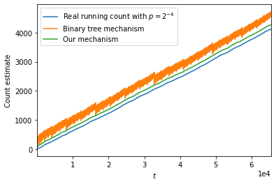
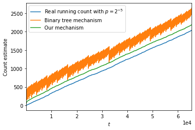
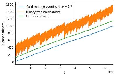
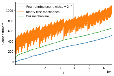
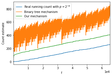
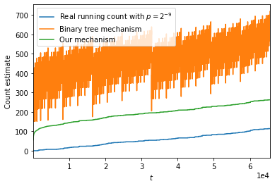
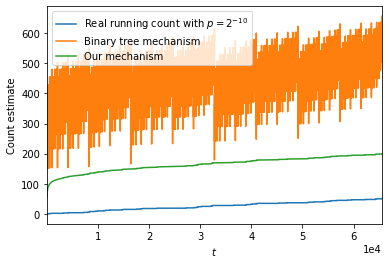
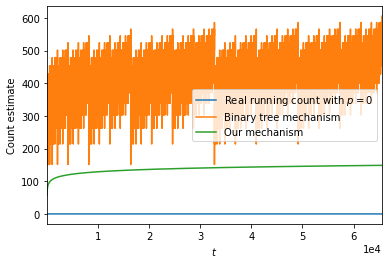
Figure 3: Comparison of our mechanism with binary mechanism for $T=2^{16},\epsilon=0.5,\delta=10^{-10}$ and various sparsity level. The $x$-axis is the current time epoch, the $y$-axis gives the output of the algorithms at each time epoch.

Results. Figure 3 shows the output of the algorithms for continual counting. Figure 4 shows the private estimate of the frequency of the most frequent item for each algorithm. On the $y$-axis, we report the output of the algorithms and the non-private output, i.e., the real count. The $x$-axis is the current time epoch.

(1) The first main takeaway is that our additive error (i.e., difference between our estimate and real count) is consistently less than that of the binary mechanism. For $t=2^{i}-1$ for $i\in\mathbb{N}$ the improvement in the additive error is factor of roughly 4. This aligns with our 1. We note that a similar observation was made in the recent work [HUU23] with respect to the $\ell_{2}$-error.

(2) The second main takeway of our experiments is that the error due to the binary mechanism is a non-smooth and a non-monotonic function of $t$ while our mechanism distributes the error smoothly and it is monotonically increasing. This can be explained from the fact that the variance of the noise in our algorithm is a monotonic function, $\ln^{2}(t)$, while that of the binary mechanism is $\ln(b)$, where $b$ is the number of ones in the bitwise representation of $t$, i.e., a non-smooth, non-monotonic function.

$p$	$2^{-4}$	$2^{-5}$	$2^{-6}$	$2^{-7}$	$2^{-8}$	$2^{-9}$	$2^{-10}$
Binary	4.72	2.40	1.12	0.61	0.31	0.15	0.072
Our mech	14.50	7.37	3.46	1.86	0.96	0.47	0.22

Table 2: Average signal to noise ratio between private estimates and true count for various sparsity level.

(3) In Table 2, we present the average SNR over all time epochs between the private estimates and the true count for different sparsity values of the stream. We notice that our output is consistently better and is about three times better when $p=2^{-10}$. We noticed that for $\epsilon=0.5,\delta=10^{-10}$ when the fraction of ones is about $1/80$, the average SNR for the binary mechanism drops below $1$, i.e., the error is larger than the true count, while for our mechanism it only drops below $1$ when the fraction of ones is $\leqslant 1/250$. That is, our mechanism can handle three times sparser streams than the binary mechanism for the same SNR. This observation continued to hold for different privacy parameters.

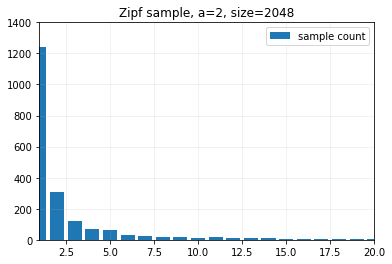
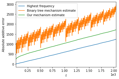
Figure 4: (Left) We give the Zipf’s law distribution that items are sampled from at each round of an event stream. (Right) the running estimate of the most frequent item using the binary mechanism and our mechanism instantiated with $\epsilon=0.1,\delta=10^{-10}$.

(4) For histogram estimation, our experiments reveal that our mechanism performs consistently better than the binary mechanism, both in terms of the absolute value of the additive error incurred as well as in terms of the smoothness of the error. This is consistent with our theoretical results. Further, on average over all time epochs, the SNR for our mechanism is $1.47$ while that of binary mechanism is $0.52$, i.e., it is a factor of about 3 better.

8 Conclusion

In this paper, we study the problem of binary counting under continual release. The motivation for this work is that (1) only an asymptotic analysis is known for the additive error for the classic mechanism (known as the binary mechanism) for binary counting under continual release, and (2) in practice the additive error is very non-smooth, which hampers its practical usefulness. Thus, we ask

Is it possible to design differentially private algorithms with fine-grained bounds on the constants of the additive error?

We first observe that the matrix mechanism can actually be used for binary counting in the continual release model if the factorization uses lower-triangular matrices. Then we give an explicit factorization for $M_{\mathsf{count}}$ that fulfill the following properties:

(1) We improved a 28 years old result on $\left\|M_{\mathsf{count}}\right\|_{\mathsf{cb}}$ to give an analysis of the additive error that only has a small gap between the upper and lower bound for the counting problem. This means that the behavior of the additive error is very well understood.

(2) The additive error is a monotonic smooth function of the number of updates performed so far. In contrast, previous algorithms would either output with the error that changes non-smoothly over time, making them less interpretable and reliable.

(3) The factorization for the binary mechanism consists of two lower-triangular matrices with exactly $T$ distinct non-zero entries that follow a simple pattern so that only $O(T)$ space is needed.

(4) We show that all these properties are not just theoretical advantages, but also makes a big difference in practice (see Figure 3).

(5) Our algorithm is very simple to implement, consisting of a matrix-vector multiplication and the addition of two vectors. Simplicity is an important design principle in large-scale deployment due to one of the important goals, which is to reduce the points of vulnerabilities in a system. As there is no known technique to verify whether a system is indeed $(\epsilon,\delta)$-differentially private, it is important to ensure that a deployed system faithfully implements a given algorithm that has provable guarantee. This is one main reason for us to pick the Gaussian mechanism: it is easy to implement with floating point arithmetic while maintaining the provable guarantee of privacy. Further, the privacy guarantee can be easily stated in the terms of concentrated-DP or Renyi-DP.

Finally, we show that our bounds have diverse applications that range from binary counting to maintaining histograms, various graph functions, outputting a synthetic graph that maintains the value of all cuts, substring counting, and episode counting. We believe that there are more applications of our mechanism, and this work will bring more attention to leading constants in the analysis of differentially private algorithms.

Acknowledgements

This project has received funding from the European Research Council (ERC) under the European Union’s Horizon 2020 research and innovation programme (Grant agreement

No. 101019564 “The Design of Modern Fully Dynamic Data Structures (MoDynStruct)” and from the Austrian Science Fund (FWF) project “Fast Algorithms for a Reactive Network Layer (ReactNet)”, P 33775-N, with additional funding from the netidee SCIENCE Stiftung, 2020–2024. JU’s research was funded by Decanal Research Grant. The authors would like to thank Rajat Bhatia, Aleksandar Nikolov, Rasmus Pagh, Vern Paulsen, Ryan Rogers, Thomas Steinke, Abhradeep Thakurta, and Sarvagya Upadhyay for useful discussions.

References

- [AFKT21] Hilal Asi, Vitaly Feldman, Tomer Koren, and Kunal Talwar. Private stochastic convex optimization: Optimal rates in l1 geometry. In International Conference on Machine Learning, pages 393–403. PMLR, 2021.
- [AFKT22] Hilal Asi, Vitaly Feldman, Tomer Koren, and Kunal Talwar. Private online prediction from experts: Separations and faster rates. arXiv preprint arXiv:2210.13537, 2022.
- [AFT22] Hilal Asi, Vitaly Feldman, and Kunal Talwar. Optimal algorithms for mean estimation under local differential privacy. arXiv preprint arXiv:2205.02466, 2022.
- [App21] Apple. https://covid19.apple.com/contacttracing, 2021.
- [Ben77] G Bennett. Schur multipliers. 1977.
- [BFM+13] Jean Bolot, Nadia Fawaz, Shan Muthukrishnan, Aleksandar Nikolov, and Nina Taft. Private decayed predicate sums on streams. In Proceedings of the 16th International Conference on Database Theory, pages 284–295. ACM, 2013.
- [BG00] Albrecht Böttcher and Sergei M Grudsky. Toeplitz matrices, asymptotic linear algebra and functional analysis, volume 67. Springer, 2000.
- [BNS19] Mark Bun, Jelani Nelson, and Uri Stemmer. Heavy hitters and the structure of local privacy. ACM Transactions on Algorithms, 15(4):51, 2019.
- [BNSV15] Mark Bun, Kobbi Nissim, Uri Stemmer, and Salil Vadhan. Differentially private release and learning of threshold functions. In 2015 IEEE 56th Annual Symposium on Foundations of Computer Science, pages 634–649. IEEE, 2015.
- [BS15] Raef Bassily and Adam Smith. Local, private, efficient protocols for succinct histograms. In Proceedings of the forty-seventh annual ACM symposium on Theory of computing, pages 127–135. ACM, 2015.
- [BW18] Borja Balle and Yu-Xiang Wang. Improving the gaussian mechanism for differential privacy: Analytical calibration and optimal denoising. In International Conference on Machine Learning, pages 394–403. PMLR, 2018.
- [CCMRT22] Christopher A Choquette-Choo, H Brendan McMahan, Keith Rush, and Abhradeep Thakurta. Multi-epoch matrix factorization mechanisms for private machine learning. arXiv preprint arXiv:2211.06530, 2022.
- [CDC20] CDC. https://www.cdc.gov/coronavirus/2019-ncov/daily-life-coping/contact-tracing.html, 2020.
- [CLSX12] T-H Hubert Chan, Mingfei Li, Elaine Shi, and Wenchang Xu. Differentially private continual monitoring of heavy hitters from distributed streams. In International Symposium on Privacy Enhancing Technologies Symposium, pages 140–159. Springer, 2012.
- [CQ05] Chao-Ping Chen and Feng Qi. The best bounds in wallis? inequality. Proceedings of the American Mathematical Society, 133(2):397–401, 2005.
- [CR21] Adrian Cardoso and Ryan Rogers. Differentially private histograms under continual observation: Streaming selection into the unknown. arXiv preprint arXiv:2103.16787, 2021.
- [CSS11] T.-H. Hubert Chan, Elaine Shi, and Dawn Song. Private and continual release of statistics. ACM Trans. Inf. Syst. Secur., 14(3):26:1–26:24, 2011.
- [Dav84] Kenneth R Davidson. Similarity and compact perturbations of nest algebras. 1984.
- [DJW13] John C Duchi, Michael I Jordan, and Martin J Wainwright. Local privacy and statistical minimax rates. In 2013 IEEE 54th Annual Symposium on Foundations of Computer Science, pages 429–438. IEEE, 2013.
- [DMR+22] Sergey Denisov, Brendan McMahan, Keith Rush, Adam Smith, and Abhradeep Thakurta. Improved differential privacy for sgd via optimal private linear operators on adaptive streams. arXiv preprint arXiv:2202.08312, 2022.
- [DNPR10] Cynthia Dwork, Moni Naor, Toniann Pitassi, and Guy N. Rothblum. Differential privacy under continual observation. In Proceedings of the 42nd ACM Symposium on Theory of Computing, pages 715–724, 2010.
- [DNRR15] Cynthia Dwork, Moni Naor, Omer Reingold, and Guy N Rothblum. Pure differential privacy for rectangle queries via private partitions. In International Conference on the Theory and Application of Cryptology and Information Security, pages 735–751. Springer, 2015.
- [DR14] Cynthia Dwork and Aaron Roth. The algorithmic foundations of differential privacy. Foundations and Trends® in Theoretical Computer Science, 9(3–4):211–407, 2014.
- [EKKL20] Marek Eliáš, Michael Kapralov, Janardhan Kulkarni, and Yin Tat Lee. Differentially private release of synthetic graphs. In Proceedings of the Annual Symposium on Discrete Algorithms, pages 560–578. SIAM, 2020.
- [EMM+23] Alessandro Epasto, Jieming Mao, Andres Munoz Medina, Vahab Mirrokni, Sergei Vassilvitskii, and Peilin Zhong. Differentially private continual releases of streaming frequency moment estimations. arXiv preprint arXiv:2301.05605, 2023.
- [ENU20] Alexander Edmonds, Aleksandar Nikolov, and Jonathan Ullman. The power of factorization mechanisms in local and central differential privacy. In Proceedings of the 52nd Annual ACM SIGACT Symposium on Theory of Computing, pages 425–438, 2020.
- [FHO21] Hendrik Fichtenberger, Monika Henzinger, and Wolfgang Ost. Differentially private algorithms for graphs under continual observation. In 29th Annual European Symposium on Algorithms, ESA 2021, September 6-8, 2021, Lisbon, Portugal (Virtual Conference), 2021.
- [Fie73] Miroslav Fiedler. Algebraic connectivity of graphs. Czechoslovak mathematical journal, 23(2):298–305, 1973.
- [Haa80] Uffe Haagerup. Decomposition of completely bounded maps on operator algebras, 1980.
- [Hon15] James Honaker. Efficient use of differentially private binary trees. Theory and Practice of Differential Privacy (TPDP 2015), London, UK, 2015.
- [HP93] Uffe Haagerup and Gilles Pisier. Bounded linear operators between -algebras. Duke Mathematical Journal, 71(3):889–925, 1993.
- [HQYC21] Ziyue Huang, Yuan Qiu, Ke Yi, and Graham Cormode. Frequency estimation under multiparty differential privacy: One-shot and streaming. arXiv preprint arXiv:2104.01808, 2021.
- [HUU23] Monika Henzinger, Jalaj Upadhyay, and Sarvagya Upadhyay. Almost tight error bounds on differentially private continual counting. SODA, 2023.
- [JRSS21] Palak Jain, Sofya Raskhodnikova, Satchit Sivakumar, and Adam Smith. The price of differential privacy under continual observation. arXiv preprint arXiv:2112.00828, 2021.
- [KMS+21] Peter Kairouz, Brendan McMahan, Shuang Song, Om Thakkar, Abhradeep Thakurta, and Zheng Xu. Practical and private (deep) learning without sampling or shuffling. In International Conference on Machine Learning, pages 5213–5225. PMLR, 2021.
- [LMH+15] Chao Li, Gerome Miklau, Michael Hay, Andrew McGregor, and Vibhor Rastogi. The matrix mechanism: optimizing linear counting queries under differential privacy. The VLDB journal, 24(6):757–781, 2015.
- [LQW14] Shukuan Lin, Jianzhong Qiao, and Ya Wang. Frequent episode mining within the latest time windows over event streams. Applied intelligence, 40(1):13–28, 2014.
- [Mat93] Roy Mathias. The hadamard operator norm of a circulant and applications. SIAM journal on matrix analysis and applications, 14(4):1152–1167, 1993.
- [MMHM21] Ryan McKenna, Gerome Miklau, Michael Hay, and Ashwin Machanavajjhala. Hdmm: Optimizing error of high-dimensional statistical queries under differential privacy. arXiv preprint arXiv:2106.12118, 2021.
- [MN12] Shanmugavelayutham Muthukrishnan and Aleksandar Nikolov. Optimal private halfspace counting via discrepancy. In Proceedings of the forty-fourth annual ACM symposium on Theory of computing, pages 1285–1292, 2012.
- [MNT20] Jiří Matoušek, Aleksandar Nikolov, and Kunal Talwar. Factorization norms and hereditary discrepancy. International Mathematics Research Notices, 2020(3):751–780, 2020.
- [Pau82] Vern I Paulsen. Completely bounded maps on -algebras and invariant operator ranges. Proceedings of the American Mathematical Society, 86(1):91–96, 1982.
- [Pau86] Vern I Paulsen. Completely bounded maps and dilations. New York, 1986.
- [RN10] Vibhor Rastogi and Suman Nath. Differentially private aggregation of distributed time-series with transformation and encryption. In Proceedings of SIGMOD International Conference on Management of data, pages 735–746, 2010.
- [Sch11] Jssai Schur. Remarks on the theory of restricted "a ned bilinear forms with infinitely many ä mutable ones. 1911.
- [STU17] Adam Smith, Abhradeep Thakurta, and Jalaj Upadhyay. Is interaction necessary for distributed private learning? In IEEE Symposium on Security and Privacy, 2017.
- [Tha17] Abhradeep Thakurta. Differential privacy: From theory to deployment, https://www.youtube.com/watch?v=Nvy-TspgZMs&t=2320s&ab_channel=USENIX, 2017.
- [Upa19] Jalaj Upadhyay. Sublinear space private algorithms under the sliding window model. In International Conference on Machine Learning, pages 6363–6372, 2019.
- [UU21] Jalaj Upadhyay and Sarvagya Upadhyay. A framework for private matrix analysis in sliding window model. In International Conference on Machine Learning, pages 10465–10475. PMLR, 2021.
- [UUA21] Jalaj Upadhyay, Sarvagya Upadhyay, and Raman Arora. Differentially private analysis on graph streams. In International Conference on Artificial Intelligence and Statistics, pages 1171–1179. PMLR, 2021.
- [WCZ+21] Tianhao Wang, Joann Qiongna Chen, Zhikun Zhang, Dong Su, Yueqiang Cheng, Zhou Li, Ninghui Li, and Somesh Jha. Continuous release of data streams under both centralized and local differential privacy. In Proceedings of the 2021 ACM SIGSAC Conference on Computer and Communications Security, pages 1237–1253, 2021.
- [Zei16] Ofer Zeitouni. Gaussian fields, 2016.
- [Zip16] George Kingsley Zipf. Human behavior and the principle of least effort: An introduction to human ecology. Ravenio Books, 2016.