Real Time Adaptive Estimation of Li-ion Battery Bank Parameters

Abstract

This paper proposes an accurate and efficient Universal Adaptive Stabilizer (UAS) based online parameters estimation technique for a 400 V Li-ion battery bank. The battery open circuit voltage, parameters modeling the transient response, and series resistance are all estimated in a single real-time test. In contrast to earlier UAS based work on individual battery packs, this work does not require prior offline experimentation or any post-processing. Real time fast convergence of parameters’ estimates with minimal experimental effort enables self-update of battery parameters in run-time. The proposed strategy is mathematically validated and its performance is demonstrated on a 400 V, 6.6 Ah Li-ion battery bank powering the induction motor driven prototype electric vehicle (EV) traction system.

I Introduction

High energy density and low self-discharge rate have made Li-ion batteries a premium candidate for electric vehicle (EV) applications. Accurate estimation of open circuit voltage (OCV), series resistance, and State-of-Charge (SoC) are indispensable for an effective battery management system. Precise estimates of internal states of a Li-ion battery like SoC, State-of-Health (SoH) also rely on an accurate battery model. The Chen and Mora equivalent circuit model [CM] has been widely adopted in the literature for Li-ion battery modeling. The salient features of this model which make it attractive for the proposed work are: it can model real time voltage and current dynamics; can capture temperature effects and number of charge-discharge cycles; it is simple to implement for a run-time battery management system; has low computational effort, and it includes SoC dependent equivalent circuit elements without requiring to solve partial differential equations (PDEs) common in electrochemical Li-ion battery models. Therefore, Chen and Mora’s battery model [CM] has been utilized for this and our previous work [Daniyal, ISMA, Access]. Different strategies are available in the literature for extracting Li-ion battery model parameters [R1, R2, R3, R4, R5, R6, new1, new2, new3, new4, new5, new6].

Not so long ago, dual unscented Kalman filter [R1] and $H_{\infty}$ Kalman filter [R2] based approaches were proposed to overcome the limitations of Kalman Filters (KFs) and Extended Kalman Filters (EKFs) for accurate battery SoC estimation. Usually, model-based KF and EKF methods require prior knowledge of battery parameters via some offline method, which is normally time-consuming and could be prone to error. However, the strategies presented in [R1], and [R2] simultaneously identify both the battery model circuit elements and SoC. A fractional calculus theory-based intuitive and highly accurate fractional-order equivalent circuit model of Li-ion battery is presented in [R3]. The fractional-order circuit is capable of modeling many electrochemical aspects of a Li-ion battery, which are typically ignored by integer-order RC equivalent circuit models. The authors in [R3] used a modified version of Particle Swarm Optimization algorithm for accurate estimation of equivalent circuit elements, and validated their results for various operating conditions of a Li-ion battery. Yet this strategy requires a precise knowledge of open circuit voltage, and optimization based strategies can be susceptible to high computational effort. The authors in [R4] proposed a moving window based least squares method for reducing the complexity and computational cost of online equivalent circuit elements’ identification, along with the battery SoC estimation. The technique presented in [R4] utilizes a piece-wise linear approximation of the open circuit voltage curve. Nevertheless, the length of the linear approximation window may affect the overall accuracy of the estimated equivalent circuit elements. The authors in [R5] attempted to identify the equivalent circuit elements of a Li-ion battery model by means of voltage relaxation characteristics. Although the strategy described in [R5] requires several pulse charging and discharging experiments, yet it extracts the equivalent circuit elements with good accuracy. A possible drawback of this strategy includes offline identification, and similar to other techniques described earlier, it relies on accurate open circuit voltage measurement. Two extended Kalman filters (named as dual EKF) are combined in [R6] for simultaneous estimation of Li-ion battery model parameters and SoC. A dead-zone is utilized in [R6] to overcome the issue of dual EKF’s high computational cost. The dead-zone defines the duration for which adaptive estimation of parameters and SoC is stopped, while the terminal voltage estimation error stays within the user-defined error limit. However, the accuracy of estimated parameters and open circuit voltage are not analyzed in [R6].

TABLE I: Comparison of important attributes for the implementation of real-time battery parameters estimation strategy.

Techniques No prior knowledge /pre-processing Determines open-circuit voltage Low computation time Ease of assuring convergence of estimate close to actual values Kalman filtering-based approaches [R1, R2, R6] $\times$ $\times$ $\checkmark$ $\checkmark$ Least squares-based approaches [new1, new2, new3] $\times$ $\checkmark$ $\checkmark$ $\times$ Metaheuristic optimization (PSO, GN) [R3], [new4] $\times$ $\checkmark$ $\times$ $\times$ Artificial intelligence-based approaches [new6] $\times$ $\checkmark$ $\times$ $\times$ Proposed UAS-based approach $\checkmark$ $\checkmark$ $\checkmark$ $\checkmark$

As for more recent methods, a variable time window-based least squares method in [new1] models the hysteresis effect and effectively captures the nonlinear dynamics of a Li-ion battery. Similarly, a partial adaptive forgetting factor-based least squares method is proposed in [new2] for Li-ion battery parameters estimation in electric vehicles. The method in [new2] also incorporates different exogenous factors such as driver behavior, environmental conditions, and traffic congestion in problem formulation. Likewise, a trust region optimization-based least squares approach is proposed in [new3], which claims to reduce the complexity, and thus the estimation time, of a conventional least squares estimation procedure. To overcome the potential limitations of Genetic Algorithm (GN), such as higher computational efforts, and possible convergence to local minima, the authors in [new4] deployed Particle Swarm Optimization (PSO) routine after GN for accurate identification of both temperature and SoC dependent Li-ion battery parameters. PSO routine not only helps to obtain a near global solution but also refines the GN results. Recently, a sequential algorithm based on high pass filter and active current injections is developed in [new5] for accurate and quick estimation of Li-ion battery parameters. It is shown in [new5] that higher frequencies in an injected current improves the performance of parameters estimation process. Various Neural Network (NN)-based data-driven strategies have also been reported in the literature for Li-ion battery parameters estimation. Different variants of NN-based methods, such as [new6] learn and capture the dynamics of a Li-ion battery model. However, the major downsides of several recent state-of-the-art methods [new1]-[new4] include some kind of offline pre-processing for appropriate selection of initial parameters, offline open-circuit voltage determination, appropriate tuning of optimization parameters, higher computational efforts, and unsatisfactory convergence performance. Moreover, some additional constraints in the recent mainstream methods are as follows. The Hessian matrix approximation undermines the accuracy of GN algorithm in [new4], the exogenous factors in [new2] are not easily accessible, and the battery current profile in [5] cannot be altered to inject the signal enriched with enough frequencies. The performance of NN-based methods [new6] relies on effective training with large datasets, requiring large memory and high computations, which may be infeasible in many battery management systems (BMS) and real-time EV applications. Furthermore, the training datasets may not be enriched with rarely occurring instances in a Li-ion battery, such as short circuit, overcharging, and overdischarging.

To highlight the advantages of the proposed UAS-based scheme compared to the mainstream methods, we present a comparative analysis of different techniques in Table I below. The attributes in Table I are considered important for real-time battery parameters estimation of an electric vehicle. An effective online strategy for battery parameters estimation should have the following attributes: (i) does not require any prior knowledge for parameters initialization or offline pre-processing, (ii) determines open-circuit voltage without offline experimentations, (iii) has low computation cost, and (iv) guarantees parameters convergence. Based on the experimental work presented in this paper, the proposed UAS-based scheme features the above-mentioned attributes and, thus, is best suitable for real-time battery parameters estimation of an electric vehicle.

This work proposes a UAS-based adaptive parameters estimation scheme for a Li-ion battery that neither needs any kind of offline pre-processing. Unlike optimization and NN-based methods, the proposed method requires very less memory and low computations, and thus it is very quick and yet effective for BMS and real-time EV applications. The proposed method has been tested and verified at the battery cell, pack and bank levels for simultaneous estimation of battery parameters, and open circuit voltage. This work utilizes a high-gain universal adaptive stabilization (UAS) based observer. The switching function required by UAS [Ilchmann] is realized by a Nussbaum function. A Nussbaum function has rapid oscillations and variable frequency by definition [Ilchmann]. When a Nussbaum function is input to the observer, it injects enough sinusoids into the high-gain observer, satisfying the required persistence of excitation (PE) condition [sastry2013]. Therefore, our previous [Daniyal, usman2019, VCollapse, alkhawaja2018] and the present work are theoretically and experimentally verified without explicitly mathematically imposing the PE condition. The above mentioned properties of a Nussbaum function result in accurate parameter estimation, even without mathematically imposing PE. It is also worth noting that some other work [stanislav2015] also exists in the literature which does not explicitly impose PE condition for parameters estimation.

This work extends our previous work [Daniyal] to another level, by estimating Li-ion battery open circuit voltage, series resistance and other battery model parameters, all by a single experiment conducted in real-time. The proposed approach is validated at the battery cell level as well as on a prototype battery bank setup for an EV traction system. In our previous work, open circuit voltage and series resistance parameters were found by the voltage relaxation test and curve fitting, respectively, and then the remaining parameters were estimated using a UAS based strategy. The previous offline adaptive parameters estimation (APE) strategy in [Daniyal] required eight experiments to estimate all battery model parameters, while the proposed online APE scheme runs online requiring only one experiment for parameters estimation. Furthermore, in contrast to [R1, R2, R3, R4, R5, R6], our proposed strategy does not require any experimental effort towards acquiring prior knowledge of open circuit voltage, rather the open circuit voltage is also estimated by the strategy proposed in this paper.

Following are the main contributions of this research work.

• The proposed online APE scheme estimates all equivalent circuit elements, including open circuit voltage, and series resistance of a Li-ion battery model at the cell/pack/bank level in one real-time experimental run.

• The proposed strategy is formulated and proved mathematically.

• The accuracy of parameters estimation is validated by the following simulations and experiments:

  • The parameters estimated in simulation using the proposed online APE approach are compared against the ones experimentally obtained by Chen and Mora [CM] for a 4.1 V, 270 mAh Li-ion battery.

  • The parameters estimated online using experimental data are compared with the previous offline parameters estimation [Daniyal] results for a 22.2 V, 6.6 Ah Li-ion battery.

  • Finally, the proposed online APE strategy is implemented on a 400 V, 6.6 Ah Li-ion battery bank powering a prototype EV traction system.

The rest of the article is organized as follows. Necessary background information about the CM [CM] Li-ion battery equivalent circuit model and UAS are provided in Section II. Section III formulates the proposed UAS based high gain adaptive observer for parameters estimation. Section LABEL:sec4 provides mathematical justification of our proposed method. Simulation and experimental results are presented in Section LABEL:sec5 and LABEL:sec6 respectively for validating the proposed online APE strategy. Real time implementation results for an EV traction system are shared in Section LABEL:sec7. Finally, the concluding remarks are made in Section LABEL:sec8 of this article.

II Background

This section provides information about the CM Li-ion battery equivalent circuit model and UAS used in this work. The battery equivalent circuit model is described in Section 2.1, while Section 2.2 presents the formulation of a Nussbaum type switching function employed in the proposed online APE algorithm.

II-A Li-ion Battery Equivalent Circuit Model

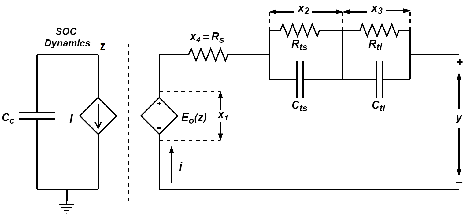
Figure 1: Li-ion battery equivalent circuit model.

The Chen and Mora [CM] equivalent circuit model of a Li-ion battery is shown in Figure 1. This work aims at providing an accurate and simple online adaptive parameters estimation method, for a battery at the cell/pack/bank level using the Li-ion battery model shown in Figure 1. The state space representation of Figure 1 is described by (1)-(6).

$$\dot{z}(t) =-\frac{1}{C_{c}}i(t),\,\,\,\,C_{c}=3600Cf_{1}f_{2}f_{3}$$ (1)

$$\dot{x}_{1}(t) =\frac{\partial x_{1}(z)}{\partial z(t)}\dot{z}(t),\mbox{ therefore}$$

$$\dot{x}_{1}(t) =-\bigg{(}r_{1}r_{2}e^{-r_{2}z}+r_{4}-2r_{5}z+3r_{6}z^{2}\bigg{)}\frac{i(t)}{C_{c}}$$ (2)

$$\dot{x}_{2}(t) =-\frac{x_{2}(t)}{R_{ts}(z)C_{ts}(z)}+\frac{i(t)}{C_{ts}(z)}$$ (3)

$$\dot{x}_{3}(t) =-\frac{x_{3}(t)}{R_{tl}(z)C_{tl}(z)}+\frac{i(t)}{C_{tl}(z)}$$ (4)

$$\dot{x}_{4}(t) =\frac{\partial x_{4}(z(t))}{\partial z(t)}\dot{z}(t)=\bigg{(}r_{19}r_{20}e^{-r_{20}}z\bigg{)}\frac{i(t)}{C_{c}}$$ (5)

$$y(t) =x_{1}(z)-x_{2}(t)-x_{3}(t)-i(t)x_{4}(t).$$ (6)

Here, the battery SoC is denoted by $z\in[0,1]$. The states $x_{1}$, $x_{2}$, $x_{3}$, $x_{4}$, represent the open circuit voltage, the voltage across $R_{ts}||C_{ts}$, the voltage across $R_{tl}||C_{tl}$, and the battery series resistance $R_{s}$ respectively. The term $C_{c}$ and $y(t)$ denote the battery capacity in ampere-hour (Ah) and battery terminal voltage. The factors $f_{1}$, $f_{2}$, $f_{3}\in[0,1]$ account for the effects of temperature, charge-discharge cycles, and self discharging respectively. The battery open circuit voltage $x_{1}$ in (2), battery series resistance $x_{4}$ in (5), and equivalent circuit elements $R_{ts},R_{tl},C_{ts},C_{tl}$ can be defined from Chen and Mora’s work [CM] by (7)-(12). Note that the formulation in (1)-(5) is novel compared to [Daniyal], as the notation introduced here for the CM model specifically allows simultaneous online estimation of battery parameters, and open circuit voltage.

$$E_{o}(z)=-r_{1}e^{-r_{2}z}+r_{3}+r_{4}z-r_{5}z^{2}+r_{6}z^{3}=x_{1}(z)$$ (7)

$$R_{ts}(z)=r_{7}e^{-r_{8}z}+r_{9}$$ (8)

$$R_{tl}(z)=r_{10}e^{-r_{11}z}+r_{12}$$ (9)

$$C_{ts}(z)=-r_{13}e^{-r_{14}z}+r_{15}$$ (10)

$$C_{tl}(z)=-r_{16}e^{-r_{17}z}+r_{18}$$ (11)

$$R_{s}(z)=r_{19}e^{-r_{20}z}+r_{21}=x_{4}(z).$$ (12)

The parameters $r_{1},\cdots,r_{21}$ used in the circuit elements in equation (7)-(12) are constant real numbers.

II-B Universal Adaptive Stabilization

The UAS based strategy has been employed in [VCollapse] for fast error convergence. This motivated us to employ the UAS based adaptive estimation method for quick [VCollapse] and yet accurate [Daniyal, Access, usman2019] Li-ion battery parameters ($r_{1},\cdots,r_{21}$) estimation. The implementation of a UAS based technique requires a switching function with high growth rate [Ilchmann]. A Nussbaum function is a switching function, which is defined as a piecewise right continuous function $N(\cdot):[k^{{}^{\prime}},\infty)\to\mathbb{R}$, $k_{0}>k^{{}^{\prime}}$, that satisfies (13) and (14).

$$\underset{k>k_{0}}{\mathrm{sup}}\,\,\frac{1}{k-k_{0}}\int\limits_{k_{0}}^{k}N(\tau)d\tau=+\infty,$$ (13)

$$\underset{k>k_{0}}{\mathrm{inf}}\,\,\frac{1}{k-k_{0}}\int\limits_{k_{0}}^{k}N(\tau)d\tau=-\infty.$$ (14)

Here, $k_{o}\in(k^{{}^{\prime}},\infty)$. In this work a Nussbaum type switching function has been implemented using the Mittag-Leffler (ML) function, described by (15).

$$E_{\alpha}(\rho)=\sum_{k=0}^{\infty}\frac{\rho^{k}}{\Gamma(k\alpha+1)},$$ (15)

Here $\Gamma(\rho+1)=\rho\Gamma(\rho),\rho>0$ is the standard Gamma function. The Nussbaum switching function of ML type is employed in this work and in [Daniyal, Access] for UAS based adaptation strategy. If $\alpha\in(2,3]$ and $\lambda>0$ then the ML function $E_{\alpha}(-\lambda t^{\alpha})$ is a Nussbaum function [Nussbaum]. The MATLAB implementation of an ML type Nussbaum switching function can be found in [ML]. In the section III, a proposed UAS observer-based Li-ion battery model parameter estimator is described for accurate estimation of battery model parameters $r_{1},\cdots,r_{21}$.

III Proposed Adaptive Parameters Estimation Methodology of a Li-on Battery Model

This section first provides the formulation details and Algorithm to implement UAS based APE strategy. Whereas, the second section describes the operational flow of our proposed methodology.

III-A Proposed UAS based battery parameters estimation methodology

A High gain adaptive estimator for a Li-ion battery model, based on (1)-(6), is described by (16)-(21).

\begin{overpic}[scale={0.1},unit=0.5mm]{FlowChart} \par\put(14.0,85.0){ $(\ref{pf11})$ } \par\put(150.5,45.0){ $(\ref{adeq})$ } \par\put(58.0,82.0){ $(\ref{pf15})-(\ref{pf14})$ } \par\put(172.0,85.0){ $(\ref{ls1})-(\ref{ls2})$ } \par\put(85.0,12.0){ $(\ref{pf16})-(\ref{pf19})$ } \par\par\put(48.0,124.0){ $i(t)$ } \par\put(72.0,70.0){ $u(t)$ } \par\put(120.0,120.0){ $\widehat{y}(t)$ } \par\put(148.0,126.0){ $y(t)$ } \par\put(18.0,9.0){ $\widehat{z}(t)$ } \par\put(28.0,68.0){ $\widehat{R}_{ts}(\widehat{z}(t)),$ } \par\put(28.0,58.0){ $\widehat{R}_{tl}(\widehat{z}(t)),$ } \par\put(28.0,48.0){ $\widehat{C}_{ts}(\widehat{z}(t)),$ } \par\put(28.0,38.0){ $\widehat{C}_{tl}(\widehat{z}(t)).$ } \par\put(129.0,70.0){ $e(t)$ } \par\put(160.0,22.0){ $\widehat{r}_{n}(t)$ } \par\put(146.0,12.0){ $n\neq\{3,21\}$ } \par\put(192.0,23.0){ $\widehat{r}_{3}(t),$ } \par\put(192.0,13.0){ $\widehat{r}_{21}(t).$ } \par\put(100.0,98.0){ $\widehat{x}_{1}(t),\widehat{x}_{4}(t).$ } \par\par\end{overpic}

Figure 2: Flowchart of online UAS based adaptive parameters estimation of a Li-ion battery model.

$$\dot{\widehat{z}}(t) =-\frac{1}{C_{c}}i(t),\,\,\,\,C_{c}=3600Cf_{1}f_{2}f_{3}$$ (16)

$$\dot{\widehat{x}}_{1}(t) =\frac{\partial\widehat{x}_{1}(\widehat{z})}{\partial\widehat{z}(t)}\dot{\widehat{z}}(t)-u(t),\widehat{x}_{1}(t)\geq 0\mbox{, therefore giving}$$

$$\dot{\widehat{x}}_{1}(t) =-\bigg{(}\widehat{r}_{1}\widehat{r}_{2}e^{-\widehat{r}_{2}\widehat{z}}+\widehat{r}_{4}-2\widehat{r}_{5}\widehat{z}+3\widehat{r}_{6}\widehat{z}^{2}\bigg{)}\frac{i(t)}{C_{c}}-u(t),\,\,\,\,$$ (17)

$$\dot{\widehat{x}}_{2}(t) =-\frac{\widehat{x}_{2}(t)}{\widehat{R}_{ts}(\widehat{z})\widehat{C}_{ts}(\widehat{z})}+\frac{i(t)}{\widehat{C}_{ts}(z)}~{}+u(t),\,\,\,\,\widehat{x}_{2}(t)\geq 0$$ (18)

$$\dot{\widehat{x}}_{3}(t) =-\frac{\widehat{x}_{3}(t)}{\widehat{R}_{tl}(\widehat{z})\widehat{C}_{tl}(\widehat{z})}+\frac{i(t)}{\widehat{C}_{tl}(z)}~{}+u(t),\,\,\,\,\widehat{x}_{3}(t)\geq 0$$ (19)

$$\dot{\widehat{x}}_{4}(t) =\frac{\partial\widehat{x}_{4}(\widehat{z}(t))}{\partial\widehat{z}(t)}\dot{\widehat{z}}(t)+u(t)\mbox{, therefore giving}$$

$$\dot{\widehat{x}}_{4}(t) =\bigg{(}\widehat{r}_{19}\widehat{r}_{20}e^{-\widehat{r}_{20}\widehat{z}}\bigg{)}\frac{i(t)}{C_{c}}+u(t),\,\,\,\,\widehat{x}_{4}(t)\geq 0$$ (20)

$$\widehat{y}(t) =\widehat{x}_{1}(t)-\widehat{x}_{2}(t)-\widehat{x}_{3}(t)-i(t)\widehat{x}_{4}(t)$$ (21)

Here $i(t)$ is the actual battery current and $\widehat{z}(t)$ is the estimated SOC, which is the same as $z(t)$ in (1). The states $\widehat{x}_{1}$, $\widehat{x}_{2}$, $\widehat{x}_{3}$, and $\widehat{x}_{4}$ denote the estimates of open circuit voltage, voltage across $\widehat{R}_{ts}||\widehat{C}_{ts}$, $\widehat{R}_{tl}||\widehat{C}_{tl}$, and estimated series resistance respectively. For simplicity, the values of $f_{1}$, $f_{2}$, $f_{3}$ are taken as 1 in this work. The estimated voltage is represented by $\widehat{y}(t)$, whereas the estimated circuit elements are given by (22)-(27).

$$\widehat{E}_{o}(\widehat{z})=-\widehat{r}_{1}e^{-\widehat{r}_{2}\widehat{z}}+\widehat{r}_{3}+\widehat{r}_{4}\widehat{z}-\widehat{r}_{5}\widehat{z}^{2}+\widehat{r}_{6}\widehat{z}^{3}=\widehat{x}_{1}(\widehat{z})$$ (22)

$$\widehat{R}_{ts}(\widehat{z})=\widehat{r}_{7}e^{-\widehat{r}_{8}\widehat{z}}+\widehat{r}_{9}$$ (23)

$$\widehat{R}_{tl}(\widehat{z})=\widehat{r}_{10}e^{-\widehat{r}_{11}\widehat{z}}+\widehat{r}_{12}$$ (24)

$$\widehat{C}_{ts}(\widehat{z})=-\widehat{r}_{13}e^{-\widehat{r}_{14}\widehat{z}}+\widehat{r}_{15}$$ (25)

$$\widehat{C}_{tl}(\widehat{z})=-\widehat{r}_{16}e^{-\widehat{r}_{17}\widehat{z}}+\widehat{r}_{18}$$ (26)

$$\widehat{R}_{s}(\widehat{z})=\widehat{r}_{19}e^{-\widehat{r}_{20}\widehat{z}}+\widehat{r}_{21}=\widehat{x}_{4}(\widehat{z}).$$ (27)

The control input $u(t)$ of UAS based-observer is designed by employing (28)-(31).

$$e(t)=y(t)-\widehat{y}(t),$$ (28)

$$\dot{k}(t)=e^{2}(t),\,\,\,\,k(t_{0})=k_{0}$$ (29)

$$N(k(t))=E_{\alpha}(-\lambda k(t)^{\alpha}),$$ (30)

$$u(t)=-N(k(t))e(t).$$ (31)

In this work, the value of $\alpha=2.5$, and $\lambda=1$ are chosen by inspection. The adaptive equation for battery parameters estimation from [Daniyal, Access], is given by (32).

$$\dot{\widehat{r}}_{n}(t)=e^{2}(t)+\lambda_{x_{n}}(r_{n_{u}}-\widehat{r}_{n}(t))+\lambda_{y_{n}}(r_{n_{l}}-\widehat{r}_{n}(t)).$$ (32)

Algorithm 1 Online UAS based algorithm for real-time adaptive parameters estimation of a Li-ion battery.

Requirements: Data acquisition circuit to measure the terminal voltage $y(t)$ and current $i(t)$ of a Li-ion battery.
Data: Initial values $\widehat{r}_{n}(0)$, upper bounds $r_{n_{u}}$, lower bounds $r_{n_{l}}$, confidence levels $\lambda_{x_{n}}$, and $\lambda_{y_{n}}$ for $n\in\{1,2,\cdots,21\}\backslash\{3,21\}$. Satisfying Lemma 4.1. Initial states $\widehat{x}_{1}(0)=E_{o}(0)$, $\widehat{x}_{2}(0)=0$, $\widehat{x}_{3}(0)=0$, $\widehat{x}_{4}(0)=0$, and $\widehat{y}(0)=y(0)$. A small positive tracking error bound $\epsilon$. Battery capacity value $C_{c}$(Ah).
Output: Estimated Li-ion battery model parameters $\widehat{r}_{1}(t)$, $\widehat{r}_{2}(t),\cdots,$ $\widehat{r}_{21}(t)$.
 

1:for $t=t_{0}:t_{step}:t_{end}$ do

2:     Read battery terminal voltage $y(t)$ and current $i(t)$.

3:     Update the error $e(t)$ using (28).

4:     Estimate battery SoC value $\widehat{z}(t)$ using (16).

5:     Evaluate (32) for $\widehat{r}_{n}(t)$ estimation, where $n\in\{1,2,\cdots,21\}\backslash\{3,21\}$.

6:     Calculate equivalent circuit element $\widehat{R}_{ts}(\widehat{z})$, $\widehat{R}_{tl}(\widehat{z})$, $\widehat{C}_{ts}(\widehat{z})$, $\widehat{C}_{tl}(\widehat{z})$ using (23)-(26).

7:     Find $u(t)$ using (31).

8:     Estimate the states $\widehat{x}_{1}(\widehat{t})$, $\widehat{x}_{2}(t)$, $\widehat{x}_{3}(t)$, $\widehat{x}_{4}(\widehat{t})$ using (17)-(20).

9:     Estimate the terminal voltage $\widehat{y}(t)$ using (21).

10:     Update the error $e(t)$ using (28).

11:     if ($|e(t)|<\epsilon$) then

12:         if $\Bigg{[}\widehat{r}_{14}(t)>-\dfrac{1}{\widehat{z}(t)}\ln{\bigg{(}\dfrac{\widehat{r}_{15}(t)}{\widehat{r}_{13}(t)}\bigg{)}}\Bigg{]}$ and $\Bigg{[}\widehat{r}_{17}(t)>-\dfrac{1}{\widehat{z}(t)}\ln{\bigg{(}\dfrac{\widehat{r}_{18}(t)}{\widehat{r}_{16}(t)}\bigg{)}}\Bigg{]}$ then

13:              Solve (LABEL:ls1) and (LABEL:ls2) to get $\widehat{r}_{3}(t)$ and $\widehat{r}_{21}(t)$.

14:              Return $\big{[}\widehat{r}_{1}(t),\widehat{r}_{2}(t),\cdots,\widehat{r}_{21}(t)\big{]}$.

15:         else

16:              Continue loop execution.

17:         end if

18:     else

19:         Continue loop execution.

20:     end if

21:end for