Neural Speech Synthesis on a Shoestring: Improving the Efficiency of LPCNet

Abstract

Neural speech synthesis models can synthesize high quality speech but typically require a high computational complexity to do so. In previous work, we introduced LPCNet, which uses linear prediction to significantly reduce the complexity of neural synthesis. In this work, we further improve the efficiency of LPCNet – targeting both algorithmic and computational improvements – to make it usable on a wide variety of devices. We demonstrate an improvement in synthesis quality while operating 2.5x faster. The resulting open-source LPCNet algorithm can perform real-time neural synthesis on most existing phones and is even usable in some embedded devices.

Index Terms— neural vocoder, LPCNet, WaveRNN

1 Introduction

Recent advances in neural vocoders, including WaveNet [1], WaveRNN [2], and SampleRNN [3] have demonstrated significant improvements over the capabilities of statistical [4] and concatenative [5] speech synthesis. This has led to improvements in text-to-speech (TTS) [6], low bitrate speech coding [7], and more.

Unfortunately, many neural vocoders – including most GAN- [8] and flow-based [9] algorithms – require a GPU for real-time synthesis, limiting their use in mobile devices. WaveRNN was one of the first algorithms to target real-time synthesis on a CPU. LPCNet uses linear prediction to improve the efficiency of WaveRNN, making it possible to perform real-time synthesis on many smartphone CPUs [10]. Even with these advances, there is still an inherent tradeoff between synthesis quality and complexity.

In this work, we improve on LPCNet with the goal of making it even more efficient in terms of quality/complexity tradeoff. We propose algorithmic improvements through hierarchical probability distribution sampling, combined with computational improvements that seek to better adapt LPCNet to existing CPU architectures.

We review LPCNet and analyze its efficiency bottlenecks in Section 2. We propose an efficient hierarchical sampling method in Section 3, which makes it possible to increase the size of the second GRU. We then propose improvements to the computational efficiency in Section 4, and discuss training aspects in Section 5. In Section 6, we evaluate the proposed improvements and demonstrate real-time synthesis for low-power embedded platforms.

2 LPCNet Overview

LPCNet is a proposed improvement to WaveRNN that makes use of linear prediction to ease the task of the RNN. It operates with pre-emphasis in the $\mu$-law domain and its output probability density function (pdf) is used to sample a white excitation signal. Using a GRU of size $N_{A}=384$, LPCNet can achieve high-quality real-time synthesis with a complexity of 3 GFLOPS, using 20% of an Intel 2.4 GHz Broadwell core [11], a significant reduction over the original WaveRNN (around 10 GFLOPS).

LPCNet includes both a frame rate network and a sampling rate network (Fig. 1). In this paper, we focus on improving the sampling rate network, which is responsible for more than 90% of the total complexity. LPCNet uses several algebraic simplifications (Section 3.6 of [10]) to avoid the operations related to the input matrix of the main GRU ($\mathrm{GRU_{A}})$, making the recurrent weights responsible for most of the total complexity. Despite that, other components contribute to the complexity, including the second GRU (addressed in  [12]), as well as the sampling process.

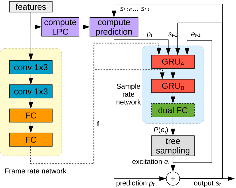
Fig. 1: Overview of the improved LPCNet vocoder proposed in this work. Compared to the original LPCNet, the softmax and direct sampling steps are replaced by a hierarchical tree sampling. Only a subset of the dual full-connected outputs is computed (as needed). Computational efficiency improvements are not shown in this figure.

As we previously reported in [11], an important bottleneck is the cache bandwidth required to load all of the sampling rate network weights for every output sample. This is compounded by the fact that these weights often do not fit in the L2 cache of CPUs. A secondary bottleneck includes about 2000 activation function evaluations per sample (for $N_{A}=384$). We propose a coherent set of improvements that jointly alleviate most of these bottlenecks.

3 Model Algorithmic Efficiency

Before addressing the computational bottlenecks listed earlier, we consider algorithmic efficiency improvements to LPCNet – both in terms of reducing complexity and in terms of improving quality for a similar complexity.

3.1 Hierarchical Probability Distribution

One area where LPCNet can be improved is in sampling its output probability distribution. In [12], the authors propose using tensor decomposition to reduce the complexity of the dual FC layer. In the “bit bunching” proposal [13], the output resolution is extended to 11 bits by splitting the output pdf into a 7-bit softmax and an additional 4-bit softmax. In this work, we keep the resolution to 8 bits ($Q=256$), but push the “bunching” idea further, splitting for every bit. This results in the output distribution being represented as an 8-level binary tree, with each branch probability being computed as a sigmoid output. Even though we still have 255 outputs in the last layer, we only need to sequentially compute 8 of them when sampling, making the sampling $O\left(\log Q\right)$ instead of $O\left(Q\right)$. The process is illustrated in Fig. 2.

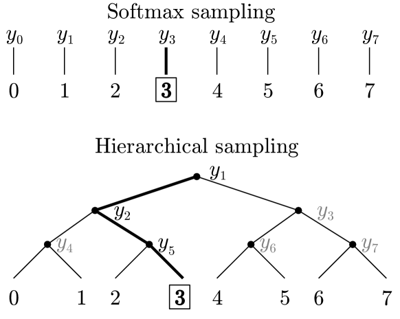
Fig. 2: Sampling example from $Q=8$ different $\mu$-law values, with $y_{i}$ being the output logits from the dual FC layer. With regular softmax sampling, all 8 $y_{i}$ values need to be evaluated to compute the partition function. With hierarchical sampling, only three $y_{i}$ values need to be evaluated (in this case, $y_{1}$, $y_{2}$, $y_{5}$) to make the branch decisions.

The hierarchical probability distribution has the other benefit of significantly reducing the number of activation function evaluations. The original LPCNet requires 512 $\tanh\left(\right)$ evaluations in the dual FC layer, and 256 $\exp\left(\right)$ evaluations in the softmax. Using hierarchical probabilities, only 16 $\tanh\left(\right)$ evaluations are required in the dual FC layer. Moreover, the 8 $\sigma\left(\right)$ evaluations for the branch probabilities can be optimized away by randomly sampling from a pre-computed table containing $\sigma^{-1}\left(r\right)$, with $r\in\left]0,1\right[$.

It is often desirable to bias the sampling against low-probability values. The original LPCNet both lowers the sampling temperature [14] on voice speech, and directly sets probabilities below a fixed threshold to zero. With hierarchical sampling, we cannot directly manipulate individual sample probabilities. Instead, each branching decision is biased to render very low probability events impossible. This can be achieved by seeding our pre-computed $\sigma^{-1}\left(r\right)$ table with $r\in\left]\xi,1-\xi\right[$. We find that $\xi=0.025$ provides natural synthesis while reducing noise and removing the occasional glitch in the synthesis.

3.2 Increasing second GRU capacity

In the original LPCNet work, $\mathrm{GRU_{B}}$ (with size $N_{B}=16$ units) acts as a bottleneck layer to avoid a high computational cost in the following dual fully-connected layer. However, with the binary tree described above reducing that complexity from $O\left(N_{B}Q\right)$ down to $O\left(N_{B}\log Q\right)$, it is now possible to double $N_{B}$ without making synthesis significantly more complex. To do that, we also make the $\mathrm{GRU_{B}}$ input matrix sparse so that the larger $\mathrm{GRU_{B}}$ does not have too many weights in its input matrix.

4 Computational Efficiency

It is also possible to improve the efficiency of LPCNet by better taking advantage of modern CPU architectures. Rather than making the model mathematically smaller, these improvements make the model run faster on existing hardware.

4.1 Weight Quantization

In the original LPCNet, $\mathrm{GRU_{A}}$ uses a block-sparse floating-point recurrent weight matrix with $16\times 1$ blocks. Recently, both Intel (x86) and ARM introduced new “dot product” instructions that can be used to compute multiple dot products of 4-dimensional 8-bit integer vectors in parallel, accumulating the result to 32-bit integer values. These can be used to efficiently compute products of $N\times 4$ matrices with $4\times 1$ vectors. For that reason, we use block-sparse matrices with $8\times 4$ blocks, with $N=8$ being chosen as a compromise between computational efficiency (larger $N$ is better) and sparseness granularity (smaller $N$ is better).

Even on CPUs where the single-instruction dot products are unavailable, they can be emulated in a way that is still more efficient than the use of 32-bit floating-point operations. Using 8-bit weights also has the advantage of both dividing the required cache bandwidth by a factor of 4 and making all of the sample rate network weights easily fit in the L2 cache of most recent CPUs. Efficient use of the cache is very important to avoid a load bottleneck since the sample rate network weights are each used only once per iteration.

To minimize the effect of quantization, we add a quantization regularization step during the last epoch of training. We use a periodic quantization regularization loss with local minima located at multiples of the quantization interval $q$:

$$\mathcal{L}_{q}=\alpha\left(1+\epsilon-\cos\frac{2\pi w}{q}\right)^{1/4}\,,$$ (1)

with $\alpha=0.01$ and $\epsilon=0.001$. We use $q=1/128$, constraining the 8-bit weights to the $\left]-1,1\right[$ range.

During the last epoch, we also gradually perform hard quantization of the weights. Weights that are close enough to a quantization point such that

$$\left|\frac{w}{q}-\left\lfloor\frac{w}{q}\right\rceil\right|<\zeta$$ (2)

are quantized to $q\left\lfloor\frac{w}{q}\right\rceil$, where $\left\lfloor\cdot\right\rceil$ denotes rounding to the nearest integer. The threshold $\zeta$ is increased linearly until $\zeta=\frac{1}{2}$, where all weights are quantized. At that point, the sample rate network weights are effectively frozen and only the biases and the (unquantized) frame rate network weights are left to adjust to the quantization process.

Weight quantization changes how the complexity is distributed among the different layers of LPCNet, especially as the GRU size changes. For small models, the complexity shifts away from the main GRU, making it possible to increase the density of $\mathrm{GRU_{A}}$ without significantly affecting the overall complexity. For large models, the activation functions start taking an increasing fraction of the complexity, again suggesting that we can increase the density at little cost.

4.2 Hyperbolic Tangent Approximation

Table 1: Rational hyperbolic tangent approximation coefficients.

$N_{0}$	1565.0352	$D_{0}$	1565.3572
$N_{1}$	158.3758	$D_{1}$	679.1774
		$D_{2}$	19.5291

As computational complexity is reduced through weight quantization and the use of sparse matrices, computing the activation functions becomes an increasingly important fraction of the total complexity. For that reason, we need a more efficient way to compute the sigmoid and hyperbolic tangent functions. We do not consider methods based on lookup tables since those are usually hard to vectorize, and although methods based on exponential approximations are viable, we are seeking an even faster method using a direct $\tanh\left(\cdot\right)$ approximation. For those reasons, we consider the Padé-inspired clipped rational function

$$\tilde{\tau}\left(x\right)=\mathrm{clip}\left(x\cdot\frac{N_{0}+N_{1}x^{2}+x^{4}}{D_{0}+D_{1}x^{2}+D_{2}x^{4}},\,-1,\,1\right)\,.$$ (3)

We optimize the $D_{k}$ and $N_{k}$ coefficients by gradient descent to minimize the maximum error $E=\max_{x}\left|\tilde{\tau}\left(x\right)-\tanh\left(x\right)\right|$ and find that the coefficients in Table 1 result in $E=6\cdot 10^{-5}$. Using Horner’s method for polynomial evaluation, the approximation in (3) can be implemented using 10 arithmetic instructions on both x86 (AVX/FMA) and ARM (NEON) architectures. Instead of the division, we use the hardware reciprocal approximation instructions, resulting in a final accuracy of $\pm 3\cdot 10^{-4}$ on x86. The error is roughly uniformly distributed, except for large input values, for which the output is exactly equal to $\pm 1$.

Since $\sigma\left(x\right)=\frac{1}{2}+\frac{1}{2}\tanh\frac{x}{2}$, the sigmoid function can be similarly approximated – still using 10 arithmetic instructions – by appropriately scaling the polynomial coefficients and adding an offset:

$$\tilde{\sigma}\left(x\right)=\mathrm{clip}\left(\frac{1}{2}+x\cdot\frac{16N_{0}+4N_{1}x^{2}+x^{4}}{64D_{0}+16D_{1}x^{2}+4D_{2}x^{4}},\,0,\,1\right)\,.$$ (4)

Again, the approximation exactly equals 0 or 1 for large input values. That is an important property for use in gated RNNs, as it allows perfect retention of the state when needed, while also avoiding the exponential growth that could occur if the gate value exceeded unity.

5 Training

The training procedure is similar to the one described in [11], with Laplace-distributed noise injected in the $\mu$-law excitation domain. To ensure robustness against unseen recording environments, we apply random spectral augmentation filtering using a second-order filter, as described in Eq. (7) of [15].

Like other auto-regressive models, LPCNet relies on teacher forcing [16] and is subject to exposure bias [17, 18]. The phenomenon becomes worse for smaller models since the decreased capacity limits the use of regularization techniques such as early stopping. We find that initializing the RNN state using the state from a random previous sequence helps the network generalize to inference. That can be easily accomplished using Tensorflow’s stateful RNN option, while still randomizing the training sequence ordering.

6 Experiments and Results

We evaluate the proposed LPCNet improvements on a speaker-independent, language-independent synthesis task where the inputs features are computed directly from a reference speech signal. All models are trained using 205 hours of 16-kHz speech from a combination of TTS datasets [19, 20, 21, 22, 23, 24, 25, 26, 27] including more than 900 speakers in 34 languages and dialects. To make the data more consistent, we ensure that all training samples have a negative polarity. This is done by estimating the skew of the residual, in a way similar to [28].

For all models, we use sequences of 150 ms (15 frames of 10 ms) and a batch size of 128 sequences. The models are trained for 20 epochs (767k updates) using Adam [29] with $\beta_{1}=0.9$ and $\beta_{2}=0.99$ and a decaying learning rate $\alpha=\frac{\alpha_{0}}{1+\delta\cdot b},$where $\alpha_{0}=0.001,$ $\delta=5\times 10^{-5}$ and $b$ is the update number. The sparse weights are obtained using the technique described in [2], with the schedule starting at $b=2,000$ and ending at $b=40,000$. As in [11], for an overall weight density $d$ in a GRU, we use $2d$ for the state weights and $d/2$ for both the update and reset gates.

We compare the proposed improvements to a baseline LPCNet [10] for different GRU sizes. The GRU sizes, $N_{A}$ and $N_{B}$, and the weight density, $d_{A}$ and $d_{B}$, are listed in Table 2, with the models named for baseline (B) or proposed (P), followed by the $\mathrm{GRU_{A}}$ size. For example, P384 is the proposed model for $N_{A}=384$.

Table 2: Definition of the models being evaluated, including the number of weights used (one multiply-add per weight) for each iteration of the sample rate network.

Model	$N_{A}$	$d_{A}$	$N_{B}$	$d_{B}$	Quantized	Weights
B192	192	0.1	16	dense	no	30k
B384	384	0.1	16	dense	no	73k
B640	640	0.1	16	dense	no	165k
P192	192	0.25	32	0.5	yes	40k
P384	384	0.1	32	0.5	yes	66k
P640	640	0.15	32	0.5	yes	219k

6.1 Complexity

Table 3: Complexity of the baseline and proposed models on x86, Neoverse N1, Cortex-A72, and Cortex-A53. The complexity is expressed as a percentage of the core compute time required for real-time synthesis (inverse of the real-time factor). A value below 100% means that the model can run in real-time on a particular core. Values in red indicate that real-time synthesis is not possible on the corresponding CPU. The speedup factor is computed as the geometric mean of the ratio over the three model sizes.

Model	x86 (%)	N1 (%)	A72 (%)	A53 (%)
B192	6.1	15.7	59	159
B384	13.2	28.5	108	277
B640	29.5	55	224	740
P192	2.8	7.1	38	92
P384	4.5	11.8	65	154
P640	11.6	26.0	150	350
Speedup	2.5x	2.2x	1.6x	1.9x

Table 4: Results from the MOS quality evaluation on both test sets, as well as the average of the two sets (overall). The confidence interval (CI) on the overall quality is 0.03 for all algorithms, except for the reference that has a CI of 0.02. All the differences in overall results are statistically significant, with $p<.01$.

Model	PTDB-TUG	NTT	Overall
Reference	4.19	4.27	4.23
Speex 4k	2.61	2.75	2.68
B192	3.63	3.65	3.64
B384	3.92	4.00	3.96
B640	3.99	4.11	4.05
P192	3.76	3.87	3.81
P384	3.93	4.07	4.00
P640	4.03	4.17	4.10

We evaluate the complexity of the proposed improvements on four different cores: an Intel i7-10810U mobile x86 core, a 2.5 GHz ARM Neoverse N1 core with similar single-core performance as recent smartphones, a 1.5 GHz ARM Cortex-A72 core similar to older smartphones, and a 1.4 GHz ARM Cortex-A53 core as found in some embedded systems.

The baseline and proposed models are implemented in C and share most of the code. Both use the same amount of hand-written AVX2 and NEON intrinsics to implement the DNN models. The measured complexity of the different models on each of the four cores is shown in Table 4. The measurements show that the computational requirement on x86 is reduced by a factor of 2.5x. In addition, the improved medium-sized model can now operate in real time on older phones ($\sim$2016), whereas the smaller model can operate on some existing low-power embedded systems.

6.2 Quality

We evaluate the models on the PTDB-TUG speech corpus [30] and the NTT Multi-Lingual Speech Database for Telephonometry. From PTDB-TUG, we use all English speakers (10 male, 10 female) and randomly pick 200 concatenated pairs of sentences. For the NTT database, we select the American English and British English speakers (8 male, 8 female), which account for a total of 192 samples (12 samples per speaker). The training material did not include any data from the datasets used in testing. In addition to the 6 models described in Table 2, we also evaluate the reference speech as an upper bound on quality, and we include the Speex 4 kb/s wideband vocoder [31] as an anchor.

The mean opinion score (MOS) [32] results were obtained using the crowdsourcing methodology described in P.808 [33]. Each file was evaluated by 20 randomly-selected listeners. The results in Table 4 show that for the same $\mathrm{GRU_{A}}$ size, the proposed models all perform significantly better than the baseline LPCNet models. The results are also consistent across the two datasets evaluated. This suggests that the small degradation in quality caused by weight quantization is more than offset by the increase in $N_{B}$ and (for P192 and P640) the density increase. Figure 3 illustrates how the proposed models affect the LPCNet quality-complexity tradeoff.

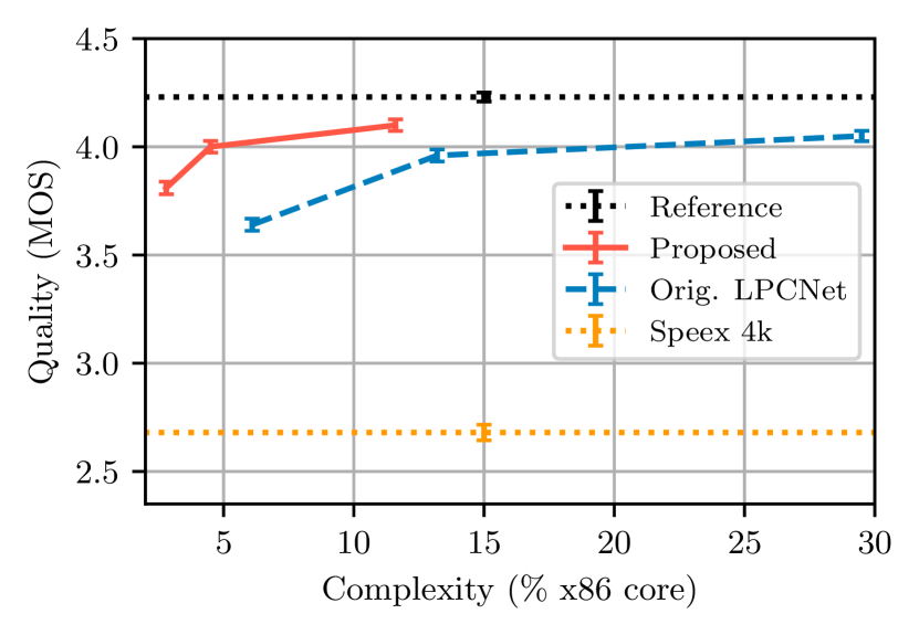
Fig. 3: Synthesis quality as a function of the complexity. We plot the x86 complexity from Table 4 with the overall quality from Table 4. The two curves approximately match when we scale the computational complexity of one of them by 3.5. This means that to obtain equal quality, the proposed method reduces the computational complexity by a factor of 3.5x.

7 Conclusion

We have proposed algorithmic and computational improvements to LPCNet. We demonstrate speed improvements of 2.5x or more, while providing better quality than the original LPCNet, equivalent to an efficiency improvement of 3.5x at equal quality. The proposed improvements make high-quality neural synthesis viable on low-power devices. Considering that the proposed changes are independent of previously proposed enhancements, such as multi-sample or multi-band sampling, we believe further improvements to the LPCNet efficiency are possible.

References

- [1] A. van den Oord, S. Dieleman, H. Zen, K. Simonyan, O. Vinyals, A. Graves, N. Kalchbrenner, A. Senior, and K. Kavukcuoglu, “WaveNet: A generative model for raw audio,” arXiv:1609.03499, 2016.
- [2] N. Kalchbrenner, E. Elsen, K. Simonyan, S. Noury, N. Casagrande, E. Lockhart, F. Stimberg, A. van den Oord, S. Dieleman, and K. Kavukcuoglu, “Efficient neural audio synthesis,” arXiv:1802.08435, 2018.
- [3] S. Mehri, K. Kumar, I. Gulrajani, R. Kumar, S. Jain, J. Sotelo, A. Courville, and Y. Bengio, “SampleRNN: An unconditional end-to-end neural audio generation model,” arXiv:1612.07837, 2016.
- [4] K. Tokuda, T. Yoshimura, T. Masuko, T. Kobayashi, and T. Kitamura, “Speech parameter generation algorithms for hmm-based speech synthesis,” in Proc. International Conference on Acoustics, Speech and Signal Processing (ICASSP), 2000, vol. 3, pp. 1315–1318.
- [5] A.J. Hunt and A.W. Black, “Unit selection in a concatenative speech synthesis system using a large speech database,” in Proc. International Conference on Acoustics, Speech and Signal Processing (ICASSP), 1996, vol. 1, pp. 373–376.
- [6] J. Shen, R. Pang, R.J. Weiss, M. Schuster, N. Jaitly, Z. Yang, Z. Chen, Y. Zhang, Y. Wang, R. Skerrv-Ryan, Y. Agiomyrgiannakis, and Y. Wu, “Natural TTS synthesis by conditioning WaveNet on Mel spectrogram predictions,” in Proc. International Conference on Acoustics, Speech and Signal Processing (ICASSP), 2018, pp. 4779–4783.
- [7] W. B. Kleijn, F. SC Lim, A. Luebs, J. Skoglund, F. Stimberg, Q. Wang, and T. C. Walters, “WaveNet based low rate speech coding,” in Proc. International Conference on Acoustics, Speech and Signal Processing (ICASSP), 2018, pp. 676–680.
- [8] C. Donahue, J. McAuley, and M. Puckette, “Adversarial audio synthesis,” in Proc. ICLR, 2019.
- [9] R. Prenger, R. Valle, and B. Catanzaro, “WaveGlow: A flow-based generative network for speech synthesis,” in Proc. International Conference on Acoustics, Speech and Signal Processing (ICASSP), 2019.
- [10] J.-M. Valin and J. Skoglund, “LPCNet: Improving neural speech synthesis through linear prediction,” in Proc. International Conference on Acoustics, Speech and Signal Processing (ICASSP), 2019, pp. 5891–5895.
- [11] J.-M. Valin and J. Skoglund, “A real-time wideband neural vocoder at 1.6 kb/s using LPCNet,” in Proc. INTERSPEECH, 2019.
- [12] H. Kanagawa and Y. Ijima, “Lightweight LPCNet-based neural vocoder with tensor decomposition,” in Proc. INTERSPEECH, 2020, pp. 205–209.
- [13] R. Vipperla, S. Park, K. Choo, S. Ishtiaq, K. Min, S. Bhattacharya, A. Mehrotra, A.G.C.P. Ramos, and N.D. Lane, “Bunched LPCNet: Vocoder for low-cost neural text-to-speech systems,” arXiv preprint arXiv:2008.04574, 2020.
- [14] Z. Jin, A. Finkelstein, G. J. Mysore, and J. Lu, “FFTNet: A real-time speaker-dependent neural vocoder,” in Proc. International Conference on Acoustics, Speech and Signal Processing (ICASSP), 2018, pp. 2251–2255.
- [15] J.-M. Valin, “A hybrid DSP/deep learning approach to real-time full-band speech enhancement,” in Proceedings of IEEE Multimedia Signal Processing (MMSP) Workshop, 2018.
- [16] R. J. Williams and D. Zipser, “A learning algorithm for continually running fully recurrent neural networks,” Neural computation, vol. 1, no. 2, pp. 270–280, 1989.
- [17] S. Bengio, O. Vinyals, N. Jaitly, and N. Shazeer, “Scheduled sampling for sequence prediction with recurrent neural networks,” in Proc. International Conference on Neural Information Processing Systems (NIPS), 2015, vol. 1, pp. 1171–1179.
- [18] M.A. Ranzato, S. Chopra, M. Auli, and W. Zaremba, “Sequence level training with recurrent neural networks,” in Proc. ICLR, 2016.
- [19] I. Demirsahin, O. Kjartansson, A. Gutkin, and C. Rivera, “Open-source Multi-speaker Corpora of the English Accents in the British Isles,” in Proc. LREC, 2020.
- [20] O. Kjartansson, A. Gutkin, A. Butryna, I. Demirsahin, and C. Rivera, “Open-Source High Quality Speech Datasets for Basque, Catalan and Galician,” in Proc. SLTU and CCURL, 2020.
- [21] K. Sodimana, K. Pipatsrisawat, L. Ha, M. Jansche, O. Kjartansson, P. De Silva, and S. Sarin, “A Step-by-Step Process for Building TTS Voices Using Open Source Data and Framework for Bangla, Javanese, Khmer, Nepali, Sinhala, and Sundanese,” in Proc. SLTU, 2018.
- [22] A. Guevara-Rukoz, I. Demirsahin, F. He, S.-H. C. Chu, S. Sarin, K. Pipatsrisawat, A. Gutkin, A. Butryna, and O. Kjartansson, “Crowdsourcing Latin American Spanish for Low-Resource Text-to-Speech,” in Proc. LREC, 2020.
- [23] F. He, S.-H. C. Chu, O. Kjartansson, C. Rivera, A. Katanova, A. Gutkin, I. Demirsahin, C. Johny, M. Jansche, S. Sarin, and K. Pipatsrisawat, “Open-source Multi-speaker Speech Corpora for Building Gujarati, Kannada, Malayalam, Marathi, Tamil and Telugu Speech Synthesis Systems,” in Proc. LREC, 2020.
- [24] Y. M. Oo, T. Wattanavekin, C. Li, P. De Silva, S. Sarin, K. Pipatsrisawat, M. Jansche, O. Kjartansson, and A. Gutkin, “Burmese Speech Corpus, Finite-State Text Normalization and Pronunciation Grammars with an Application to Text-to-Speech,” in Proc. LREC, 2020.
- [25] D. van Niekerk, C. van Heerden, M. Davel, N. Kleynhans, O. Kjartansson, M. Jansche, and L. Ha, “Rapid development of TTS corpora for four South African languages,” in Proc. Interspeech, 2017.
- [26] A. Gutkin, I. Demirşahin, O. Kjartansson, C. Rivera, and K. Túbọ̀sún, “Developing an Open-Source Corpus of Yoruba Speech,” in Proc. INTERSPEECH, 2020.
- [27] E. Bakhturina, V. Lavrukhin, B. Ginsburg, and Y. Zhang, “Hi-Fi Multi-Speaker English TTS Dataset,” arXiv preprint arXiv:2104.01497, 2021.
- [28] T. Drugman, “Residual excitation skewness for automatic speech polarity detection,” IEEE Signal Processing Letters, vol. 20, no. 4, pp. 387–390, 2013.
- [29] D.P. Kingma and J. Ba, “Adam: A method for stochastic optimization,” in Proc. ICLR, 2015.
- [30] G. Pirker, M. Wohlmayr, S. Petrik, and F. Pernkopf, “A pitch tracking corpus with evaluation on multipitch tracking scenario.,” in Proc. INTERSPEECH, 2011, pp. 1509–1512.
- [31] J.-M. Valin, “The speex codec manual,” 2007.
- [32] ITU-T, Recommendation P.800: Methods for subjective determination of transmission quality, 1996.
- [33] ITU-T, Recommendation P.808: Subjective evaluation of speech quality with a crowdsourcing approach, 2018.