Investigating the nature of the ultraluminous X-ray sources in the galaxy NGC 925

Abstract

Variability is a powerful tool to investigate properties of X-ray binaries (XRB), in particular for Ultraluminous X-ray sources (ULXs) that are mainly detected in the X-ray band. For most ULXs the nature of the accretor is unknown, although a few ULXs have been confirmed to be accreting at super-Eddington rates onto a neutron star (NS). Monitoring these sources is particularly useful both to detect transients and to derive periodicities, linked to orbital and super-orbital modulations. Here we present the results of our monitoring campaign of the galaxy NGC 925, performed with the Neil Gehrels Swift Observatory. We also include archival and literature data obtained with Chandra, XMM-Newton and NuSTAR. We have studied spectra, light-curves and variability properties on days to months time-scales. All the three ULXs detected in this galaxy show flux variability. ULX-1 is one of the most luminous ULXs known, since only 10% of the ULXs exceed a luminosity of $\sim$5$\times$10⁴⁰ erg s^-1, but despite its high flux variability we found only weak spectral variability. We classify it as in a hard ultraluminous regime of super-Eddington accretion. ULX-2 and ULX-3 are less luminous but also variable in flux and possibly also in spectral shape. We classify them as in between the hard and the soft ultraluminous regimes. ULX-3 is a transient source: by applying a Lomb-Scargle algorithm we derive a periodicity of $\sim$ 126 d, which could be associated with an orbital or super-orbital origin.

1 Introduction

Ultraluminous X-ray sources (ULXs) are extragalactic, point-like and non-nuclear objects, with luminosities in excess of 10³⁹ erg s^-1, interpreted as accreting compact objects in binary systems (see e.g. Kaaret et al. 2017 for a review). While at first they were preferentially considered the ideal place to host intermediate mass black holes (IMBH, e.g. Colbert & Mushotzky 1999, Ebisuzaki et al. 2001, Farrell et al. 2009) accreting at sub-Eddington rates, they are now widely thought to be powered by super-Eddington accretion onto stellar mass compact objects like a neutron star (NS) or a black hole (BH). The ULXs are typically observed in the so called ultraluminous state (e.g. Roberts 2007; Gladstone et al. 2009), characterised by a spectral curvature at 2$-$5 keV usually coupled to a soft excess peaking in the range 0.1–0.5 keV (e.g. Gladstone et al., 2009), and at times by temporal variability on short time-scales (e.g. Heil et al., 2009; Sutton et al., 2013; Pintore et al., 2014; Middleton et al., 2015a). Confirmation that a fraction of the ULX population contains a stellar-mass compact object comes from the detection of coherent pulsations in six ULXs (Bachetti et al., 2014; Israel et al., 2017a, b; Fürst et al., 2016; Carpano et al., 2018; Rodríguez Castillo et al., 2019; Sathyaprakash et al., 2019), which can be explained only by the presence of a NS in these systems, and from the detection of a transient cyclotron line in the NS candidate M51 ULX-8 (Brightman et al., 2018). Considering that only $\sim$20 sources have enough statistics to detect pulsations (e.g. Earnshaw et al. 2019; Song et al. 2020), the NSs may be a significant fraction among the bright ULX population (Pintore et al. 2017; Koliopanos et al. 2017; Walton et al. 2018a).

The short-term (seconds to hours) temporal properties of ULXs are quite different from those observed in Galactic X-ray binary systems and are not related to specific spectral states (e.g. Heil et al., 2009): even if the amplitude of short-term variability is larger in soft ultraluminous sources than in hard ones (Sutton et al., 2013), the variability appears to be poorly predictable, i.e. it is not found in all sources with a soft spectrum and, when detected in a source, it is not necessarily found in all the observations of that ULX. Such variability was explained with the existence of optically thick and non-uniform winds, radiatively ejected by the accretion disc, which stochastically intersect our line of sight (e.g. Middleton et al. 2011, 2015a). Observational evidences of these winds come from the detection of blue-shifted absorption lines in the high quality grating spectra of some ULXs (e.g. Pinto et al. 2016; Kosec et al. 2018) and by the nebulae observed in the radio (e.g. Cseh et al. 2012), optical (e.g. Pakull et al. 2010) or X-ray band (Belfiore et al. 2020). Long-term flux variability (days to months) is also observed in most of the monitored ULXs. Such variability, in some cases, can be as high as several orders of magnitudes, implying that these sources are transients (detected at least once in the ultraluminous state, L${}_{x}>$ 10³⁹ erg s^-1, and either once at a significantly smaller luminosity or undetected below the instrumental sensitivity; e.g. Pintore et al. 2018a; Soria et al. 2012). Often the pulsating ULXs (PULXs) show large flux variations, implying they can be considered as transient ULXs. A bi-modal flux distribution is sometimes observed in the long-term light-curves of PULXs (e.g. Walton et al. 2015a; Motch et al. 2014). A possible explanation for this long-term behaviour may be the propeller effect: when the magnetospheric radius of the NS becomes larger than the corotation radius of the accreting matter in the disc, a centrifugal barrier prevents the accretion onto the NS, with a corresponding decrease in the X-ray flux (Illarionov & Sunyaev 1975; Tsygankov et al. 2016; Grebenev 2017). The propeller effect can act only if the accretor is a NS with a strong magnetic field, so a bi-modal flux distribution can be used to identify candidate PULXs, even when pulsations are not detected (e.g. Earnshaw et al. 2018; Song et al. 2020). Furthermore, long-term monitored ULXs revealed possible (super-)orbital variability (e.g. Foster et al., 2010; An et al., 2016; Fürst et al., 2018), the origin of which is still a matter of debate. Super-orbital periods are also observed in the light-curves of the PULXs, with periods of tens to hundreds days (e.g. Walton et al., 2016; Brightman et al., 2019, 2020). The detection of such long-term periodicities were only possible thanks to the flexibility and performance of the Neil Gehrels Swift Observatory (hereafter Swift; Gehrels et al. 2004).

Some ULXs present also spectral variability (see, for example, Bachetti et al. 2013; Pintore et al. 2014). Pintore et al. (2017) suggested, based on hardness ratio studies, that the known PULXs generally have harder spectra amongst the ULXs population. We use here the spectral classification in three spectral regimes proposed by Sutton et al. (2013), based on the spectral parameters of a multi-colour disc plus a power-law model: broadened disc, hard ultraluminous and soft ultraluminous. Sources with an inner disc temperature $<$ 0.5 keV are classified in the hard ultraluminous regime, if the power-law index is smaller than 2, and in the soft ultraluminous regime, if the power-law index is larger than 2. When the inner disc temperature assumes values larger than 0.5 keV, if the ratio between the power-law flux and the disc flux in the (0.3–1) keV band is larger than 5, we have again an ultraluminous regime, hard or soft depending on the power-law index. Otherwise, when the flux ratio is smaller than 5, the spectrum is characterised by a dominant disc component, and the regime is labelled as broadened disc. The broadened disc is characterised by a broad disc-like spectral shape and is very common in the lower-luminosity sources (below $\sim$ 3$\times$10³⁹ erg s^-1) but it is sometimes also observed at higher luminosities. The two ultraluminous regimes are instead characterised by two spectral components, with a peak in the higher (hard ultraluminous) or lower (soft ultraluminous) energy component of the 0.3-10 keV spectrum.

Such regimes are thought to depend both on the mass accretion rate and on the observer’s viewing angle: if the system is seen face-on, the hard inner emission is directly detected (hard-ultraluminous regime), while for more inclined systems the emission from the innermost regions is seen through the wind, appearing softer (soft-ultraluminous regime). Both ultraluminous regimes may coexist in a single system. The switching between the two regimes is determined by changes in the accretion rate driving changes in the outflowing wind opening angle (e.g. Sutton et al. 2013; Middleton et al. 2015a).

Most of the X-ray flux variability is observed in the hard band, above 1 keV, and could be associated to temporary obscuration of the hot inner disc regions by the funnel created by the puffed disc and the wind (e.g. Middleton et al. 2015a; Pinto et al. 2017). However, the rather stable hard flux above 10 keV as observed in some archetypal ULXs like NGC 1313 X-1 and Holmberg IX X-1 suggests that the scenario might be more complicated (Walton et al., 2017, 2020; Gúrpide et al., 2021a). This is confirmed by the findings of different variability patterns such as flaring activity in some hard ULXs (e.g. Motta et al. 2020; Pintore et al. 2021) and flux-dips in soft ULXs (e.g. Stobbart et al. 2004; Feng et al. 2016; Alston et al. 2021; Pinto et al. 2021; D’Aì et al. 2021). Pointed, deep observations with high-throughput telescopes are limited and cannot enable a detailed study of the long-term behaviour. This prevents us from obtaining an overall view of their accretion cycle. Swift instead allows us to perform X-ray spectroscopic studies over a long ($\sim$ yearly) baseline with weekly visits, as proved by previous studies (e.g. Kaaret & Feng, 2009; Grisé et al., 2010; La Parola et al., 2015; Brightman et al., 2020; Gúrpide et al., 2021b).

The long-term behaviour is reported only for a small fraction of the whole ULX population (e.g. Brightman et al. 2019, 2020; Gúrpide et al. 2021b), containing 1843 ULX candidates according to the recent catalogue of Walton et al. 2021. Thus, to enlarge this sample, it is crucial to perform studies of long-term variability, possibly correlated with spectral changes, and to look for periodicities. The main aim of this work is to report on the long-term properties of the ULXs in the galaxy NGC 925 (Figure 1), using data taken with a Swift/XRT monitoring. To complete our analysis we used also archival data taken with other X-ray facilities.

	RA	Dec	Chandra	ref.
ULX-1	02:27:27.5	+33:34:43.0	CXO J022727+333443	a
ULX-2	02:27:21.5	+33:35:00.7	CXO J022721+333500	a
ULX-3	02:27:20.2	+33:34:12.8		b

Table 1: Chandra coordinates of the three ULXs in the galaxy NGC 925. Column 4 lists the names of the sources detected in the Chandra catalog, while column 5 reports the first reference for each source: a) Swartz et al. 2011; b) Earnshaw et al. 2020.

NGC 925 is a spiral galaxy (SAB(s)d) at a distance of $\sim$ 8.9 Mpc (Tully et al., 2013). It contains 3 known ULXs: NGC 925 ULX-1, NGC 925 ULX-2, whose data were extensively studied in Pintore et al. (2018b), and NGC 925 ULX-3, which is a transient ULX discovered by Earnshaw et al. (2020). Their positions as measured by Chandra (Swartz et al. 2011; Earnshaw et al. 2020) are reported in Table 1.

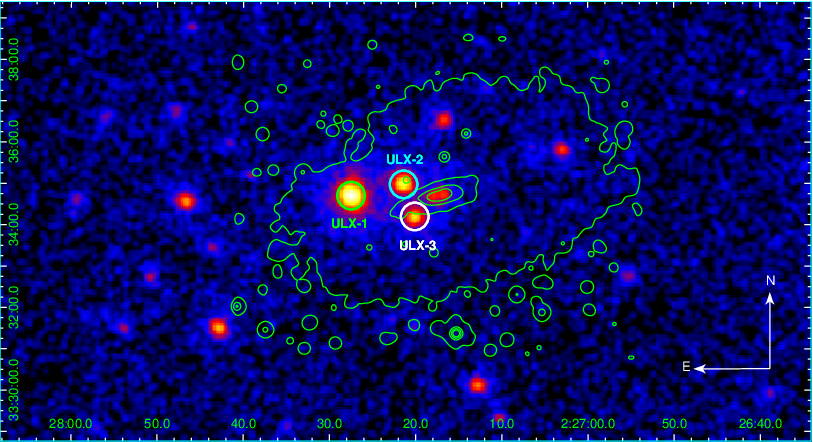
Figure 1: Stacked image from all the Swift/XRT observations analysed in this work. The coordinates of the image are expressed in RA, Dec (FK5). Positions of ULX-1, ULX-2 and ULX-3 are indicated by a green, cyan and white circle of 20^′′ radius, respectively. The optical contours of the galaxy NGC 925 from DSS are super-imposed with solid green lines for reference.

The paper is organized as follows. In Sect. 2, we describe the data used in this paper, the basic data reduction and analysis. The results for each ULX in the galaxy are reported in Sect. 3, while their implications are discussed in Sect. 4. Finally our conclusions are in Sect. 5.

Instr.	Obs.ID	Start time	Stop time	Exp
		[YYYY-MM-DD hh:mm:ss]		[ks]
1   Swift/XRT	00045596001	2011-07-21T09:26:28	2011-07-21T15:59:55	2.6
2   Swift/XRT	00045596002	2011-07-26T14:40:42	2011-07-26T14:54:55	0.8
3   Swift/XRT	00045596003	2011-07-27T00:03:18	2011-07-27T14:58:52	5.7
4   Swift/XRT	00045596004	2011-07-31T02:25:56	2011-07-31T23:19:55	0.3
5   Swift/XRT	00045596005	2011-08-02T00:58:52	2011-08-02T02:36:56	0.2
6   Swift/XRT	00045596006	2011-08-06T15:39:11	2011-08-06T15:43:56	0.3
7   Swift/XRT	00045596007	2011-09-07T03:33:50	2011-09-07T03:55:57	1.3
8   Swift/XRT	00045596008	2011-09-13T00:48:18	2011-09-13T12:09:56	3.6
9   Swift/XRT	00045596009	2012-08-23T22:06:46	2012-08-23T23:45:54	0.6
10   Swift/XRT	00045596010	2012-08-24T17:00:02	2012-08-25T14:00:55	5.3
11   Swift/XRT	00045596011	2012-08-27T20:28:20	2012-08-27T20:43:55	0.9
12   Swift/XRT	00045596012	2012-08-28T02:54:05	2012-08-28T20:28:55	4.4
13   Swift/XRT	00045596013	2012-08-29T01:16:16	2012-08-29T22:26:56	6.5
14   Swift/XRT	00045596014	2014-09-07T07:31:45	2014-09-07T09:19:54	2.1
15   Swift/XRT	00045596015	2017-11-19T05:59:52	2017-11-19T07:47:53	2.1
16   Swift/XRT	00045596016	2017-11-19T15:56:16	2017-11-19T17:27:52	1.9
17   Swift/XRT	00045596017	2017-11-21T07:45:23	2017-11-21T09:30:52	1.7
18   Swift/XRT	00045596018	2017-11-25T20:05:50	2017-11-25T22:00:54	1.8
19   Swift/XRT	00045596019	2019-08-18T16:33:23	2019-08-18T22:55:52	1.3
20   Swift/XRT	00045596020	2019-08-21T04:41:38	2019-08-21T05:02:52	1.3
21   Swift/XRT	00045596021	2019-08-25T18:33:26	2019-08-25T18:50:51	1.0
22   Swift/XRT	00045596022	2019-08-27T05:51:49	2019-08-27T21:57:53	1.5
23   Swift/XRT	00045596023	2019-09-01T05:20:20	2019-09-01T16:49:53	1.6
24   Swift/XRT	00045596024	2019-09-08T06:00:36	2019-09-09T03:01:52	2.4
25   Swift/XRT	00045596025	2019-09-15T13:27:33	2019-09-15T23:14:53	2.6
26   Swift/XRT	00045596026	2019-09-22T22:23:05	2019-09-22T22:47:52	1.5
27   Swift/XRT	00045596027	2019-09-25T22:05:20	2019-09-25T22:28:54	1.4
28   Swift/XRT	00045596028	2019-10-06T02:10:34	2019-10-06T21:28:54	1.2
29   Swift/XRT	00045596029	2019-10-09T11:29:11	2019-10-09T19:31:51	1.6
30   Swift/XRT	00045596030	2019-10-13T15:26:57	2019-10-13T17:28:52	2.9
31   Swift/XRT	00045596031	2019-10-20T06:55:11	2019-10-20T21:41:52	2.1
32   Swift/XRT	00045596032	2019-10-27T00:03:15	2019-10-27T22:35:52	2.5
33   Swift/XRT	00045596033	2019-11-03T18:17:09	2019-11-03T21:53:52	2.8
34   Swift/XRT	00045596034	2019-11-13T12:48:09	2019-11-13T22:33:53	2.8
35   Swift/XRT	00045596035	2019-11-17T06:02:31	2019-11-18T10:54:53	2.8
36   Swift/XRT	00045596036	2019-11-28T19:07:33	2019-11-28T22:43:54	2.5
37   Swift/XRT	00045596037	2019-12-08T03:37:33	2019-12-08T15:12:53	3.3
38   Swift/XRT	00089002001	2019-12-13T03:19:50	2019-12-13T05:02:54	1.9
39   Swift/XRT	00045596038	2019-12-18T12:12:51	2019-12-18T15:39:53	1.6
40   Swift/XRT	00045596039	2019-12-22T19:45:59	2019-12-22T19:53:53	0.5
41   Swift/XRT	00045596041	2020-01-02T09:15:03	2020-01-02T14:22:52	3.5
42   Swift/XRT	00045596042	2020-01-07T18:45:42	2020-01-07T22:06:52	1.2
43   Swift/XRT	00045596044	2020-03-01T21:11:49	2020-03-01T23:08:53	2.4
44   Swift/XRT	00045596045	2020-03-08T09:21:10	2020-03-08T11:21:09	2.4
45   Swift/XRT	00045596046	2020-03-15T00:37:12	2020-03-15T03:54:52	2.9
46   Swift/XRT	00095702001	2020-07-01T01:01:15	2020-07-01T09:06:53	2.1
47   Swift/XRT	00095702002	2020-07-11T04:45:24	2020-07-11T06:35:54	2.6
48   Swift/XRT	00095702003	2020-07-21T04:02:28	2020-07-21T13:45:53	1.9
49   Swift/XRT	00095702004	2020-07-31T17:17:45	2020-07-31T22:10:53	2.0
50   Swift/XRT	00095702005	2020-08-10T08:14:50	2020-08-10T10:28:53	2.6
51   Swift/XRT	00089004001	2020-08-17T07:32:05	2020-08-17T07:58:52	1.6
52   Swift/XRT	00095702006	2020-08-20T00:52:59	2020-08-20T16:55:52	2.8
53   Swift/XRT	00095702007	2020-08-30T17:18:07	2020-08-30T19:04:53	2.3
54   Swift/XRT	00095702008	2020-09-09T09:58:56	2020-09-09T12:04:52	2.5
55   Swift/XRT	00095702009	2020-09-19T10:41:53	2020-09-19T14:05:54	2.4
56   Swift/XRT	00095702010	2020-09-29T19:24:34	2020-09-29T21:16:52	2.5
57   Swift/XRT	00095702011	2020-10-08T13:35:29	2020-10-09T21:33:53	2.6
58   Swift/XRT	00095702012	2020-10-19T12:46:33	2020-10-19T12:48:54	0.1
59   Swift/XRT	00095702013	2020-10-22T12:09:32	2020-10-22T13:53:54	2.3
60   Swift/XRT	00095702014	2020-10-29T14:49:06	2020-10-29T16:32:52	1.9
61   Swift/XRT	00095702015	2020-11-08T10:40:54	2020-11-08T12:28:53	2.5
62   Swift/XRT	00095702016	2020-11-18T16:12:05	2020-11-18T22:50:54	1.5
63   Swift/XRT	00095702017	2020-11-29T13:15:24	2020-11-29T16:52:53	2.2
64   Swift/XRT	00095702018	2020-12-08T05:51:23	2020-12-08T07:48:53	2.0
65   Swift/XRT	00095702019	2020-12-18T11:15:01	2020-12-18T17:53:53	1.9
66   Swift/XRT	00095702020	2020-12-28T10:18:55	2020-12-28T10:20:26	0.1
67   Swift/XRT	00095702021	2021-01-01T06:37:39	2021-01-01T08:25:52	2.4
68   Swift/XRT	00095702022	2021-01-07T12:31:39	2021-01-07T16:08:52	2.5
69   Swift/XRT	00095702023	2021-01-17T02:01:45	2021-01-17T08:35:54	2.5
70   Swift/XRT	00095702025	2021-01-31T10:15:05	2021-01-31T13:37:53	2.3
71   Swift/XRT	00095702026	2021-02-06T13:58:46	2021-02-06T15:47:53	2.5
72   Swift/XRT	00095702027	2021-02-15T00:28:25	2021-02-16T13:37:54	2.6
73   Swift/XRT	00095702028	2021-02-26T01:04:10	2021-02-26T22:07:53	2.2
74   Swift/XRT	00095702029	2021-03-08T12:36:39	2021-03-08T14:33:53	2.4
75   Chandra	7104	2005-11-23T07:53:09	2005-11-23T08:57:05	2.2
76   Chandra	20356	2017-12-01T03:38:39	2017-12-01T07:04:06	10.0
77   XMM-N.	0784510301	2017-01-18T19:45:14	2017-01-19T09:38:34	50.0
78   NuSTAR	30201003002	2017-01-18T19:36:09	2017-01-19T17:41:09	42.6
79   NuSTAR	90501351002	2019-12-12T05:31:09	2019-12-13T11:46:09	53.0

Table 2: Log of the observations used in this work.

2 Data Reduction and Analysis

2.1 Swift/XRT

Swift/XRT pointed at the galaxy NGC 925 for 74 times between July 2011 and March 2021 (see the stacked image of all the pointings in Figure 1), with observations in PC mode of, on average, about 2 ksec. We list them, with dates of observation and relative exposures, in Tab. 2.

We reduced Swift/XRT data adopting standard procedures. We ran the xrtpipeline and we used a sliding-cell method of detection (detect command in ximage), to verify if new ULXs turned on during the Swift/XRT observations. We choose a detection threshold of 3$\sigma$ for each observation and for the stacked set of all observations listed in Table 2. However, no new ULXs were found in the D₂₅ of the galaxy (D${}_{25}\sim$ 10.7^′ from HyperLeda database).

To obtain light-curves and spectra of all the ULXs in the galaxy, we used the online tool for XRT products (Evans et al., 2009). The extraction regions have been centred on the coordinates obtained from the detection on the Swift/XRT stacked image, which are fully consistent with the Chandra coordinates. Since the minimum searching radius allowed for the centroiding (1 arcmin) is comparable with the distances among the ULXs in NGC 925, the centroiding option has been disabled, in order to avoid the possible spurious centering on the wrong ULX. We also created an average Swift/XRT spectrum for each ULX, from the stacked image.

2.2 Chandra

Chandra/ACIS-S observed the galaxy twice on 25 November 2006 and 1st December 2018 (Obs.ID: 7104, 20356) with observing time of 2 and 10 ksec, respectively (Tab. 2).

We reduced Chandra data with CIAO v.4.11 (Fruscione et al., 2006) and used calibration files CALDB v.4.8.3. We selected source events from a circular region of 3^′′ radius (the smallest suitable radius owing to the off-axis position of the sources, especially in the first observation), while the background was chosen from annular regions with inner and outer radii of 6^′′ and 20^′′, respectively. We extracted sources and background spectra, and their response and ancillary files using the CIAO task specextract.

2.3 XMM-Newton

There is only one public XMM-Newton observation taken on 18 January 2017 at the time of the analysis (Tab. 2). We reduced the EPIC-pn and MOS data with the software SAS v17.0.0. We selected single and double pixel events for the pn (PATTERN $\leq$ 4) and single and multiple pixel events for the MOS (PATTERN $\leq$ 12). We cleaned the data to remove time intervals of high particle background, which resulted in a net exposure time of $\sim$ 32 ks (pn) and 42 ks (MOS).

We extracted source data from circular regions of 35^′′ (ULX-1) and 20^′′ (ULX-2, ULX-3) radii. We used a smaller extraction region for ULX-2 and ULX-3 to prevent contamination between the two sources, which are close to each other. ULX-2 falls into a CCD gap in the EPIC-pn, so we did not use the pn data for the spectral analysis of ULX-2. The background data were extracted from circular regions of 60^′′ radius, in a region free of contaminating sources, in the same CCD quadrant and near each source, so as to be at a similar off-axis angular distance.

2.4 NuSTAR

Two NuSTAR observations were taken in 2017 ($\sim$ 42 ks) and 2019 ($\sim$ 53 ks). We note that the first one started about 20 minutes before the 2017 XMM-Newton observation (Tab. 2).

NuSTAR data were reduced using standard procedures with nustardas v1.3.0 of the Ftools v6.16 and we used the CALDB v.20180312. The extraction region for ULX-1 was a circle of 50^′′ radius. The background was chosen from a nearby 80^′′ radius circular region, and free of sources. For ULX-2 we used a circular region of 30^′′ to limit any possible contamination from the nearby ULX-1 and ULX-3.

In 2017 only ULX-1 and ULX-2 were detected; we used the NuSTAR data in conjunction with simultaneous XMM-Newton data. In 2019, instead, also ULX-3 was bright, and the closeness to ULX-2 does not allow us to correctly disentangle the two. Therefore we used only the NuSTAR observation of ULX-1 in conjunction with three Swift/XRT observations close in time (8, 13 and 18 December 2019). We combined the latter to get a stacked, quasi-simultaneous ULX-1 spectrum to be analysed in conjunction with the NuSTAR spectrum.

2.5 Spectral analysis

Source	Epoch	n${}_{\rm H}^{int}$	kT${}_{\text{diskbb}}$	N${}_{\text{disc}}$	kT${}_{\text{bbodyrad}}$	N${}_{\text{bb}}$	Flux${}_{\text{diskbb}}$	Flux${}_{\text{bbodyrad}}$	$\chi^{2}$/dof	Pval
		$10^{22}$ cm-2	keV	10-3	keV		$10^{-13}$ erg s-1 cm-2
ULX1
	XMM	0.09${}^{+0.02}_{-0.02}$	2.3${}^{+0.1}_{-0.1}$	3.7${}^{+0.8}_{-0.7}$	0.29${}^{+0.02}_{-0.02}$	5.6${}^{+1.7}_{-1.2}$	18.5$\pm$0.4	4.1$\pm$0.1	1153.29/1131	0.32
	XMM/NuSTAR(a)	0.06${}^{+0.02}_{-0.02}$	2.8${}^{+0.1}_{-0.1}$	1.7${}^{+0.3}_{-0.3}$	0.33${}^{+0.02}_{-0.02}$	3.7${}^{+0.8}_{-0.6}$	18.0$\pm$0.4	4.7$\pm$0.1	1371.67/1269	0.02
	Chandra	0.09	2.2${}^{+0.8}_{-0.4}$	4.2${}^{+4.7}_{-2.8}$	0.3${}^{+0.1}_{-0.1}$	2.9${}^{+3.7}_{-1.6}$	19.0$\pm$2.0 / 18.8$\pm$1.1	2.3$\pm$0.7 / 2.5$\pm$0.6	70.89/63	0.29
	Swift average	0.09	2.1${}^{+0.3}_{-0.2}$	4.7${}^{+2.1}_{-1.6}$	0.3${}^{+0.1}_{-0.1}$	2.7${}^{+2.6}_{-1.2}$	17.4$\pm$0.5	1.8$\pm$0.2	181.47/206	0.81
	Swift/NuSTAR(b)	0.09	3.7${}^{+0.5}_{-0.4}$	0.2${}^{+0.1}_{-0.1}$	0.4${}^{+0.1}_{-0.1}$	0.9${}^{+1.0}_{-0.6}$	5.3$\pm$2.1	3.5$\pm$0.8	87.18/79	0.25
ULX2
	XMM/NuSTAR	0.02${}^{+0.02}_{-0.02}$	2.9${}^{+0.7}_{-0.5}$	0.2${}^{+0.2}_{-0.1}$	0.31${}^{+0.04}_{-0.04}$	1.1${}^{+1.0}_{-0.5}$	2.6$\pm$0.2	1.1$\pm$0.1	145.27/139	0.34
	Chandra	0.02	1.5${}^{+3.9}_{-0.5}$	3.1${}^{+10.1}_{-3.0}$	0.2${}^{+0.1}_{-0.1}$	3.3${}^{+12.6}_{-2.7}$	3.2$\pm$0.9 / 3.1$\pm$0.4	0.8$\pm$0.6 / 1.0$\pm$0.3	4.23/9	0.90
	Swift average	0.02	1.3${}^{+0.1}_{-0.1}$	7.3${}^{+2.0}_{-1.6}$	0.03${}^{+0.04}_{-0.03}$	$>$242.5	4.2$\pm$0.2	0.5$\pm$0.3	74.59/62	0.13
ULX3
	XMM	0.22${}^{+0.04}_{-0.03}$	1.1${}^{+0.6}_{-0.3}$	0.6${}^{+1.8}_{-0.5}$	0.12${}^{+0.02}_{-0.02}$	17.9${}^{+24.4}_{-9.9}$	0.26$\pm$0.04	0.3$\pm$0.1	40.55/38	0.36
	Chandra	0.22	1.6${}^{+0.4}_{-0.3}$	4.0${}^{+3.1}_{-2.4}$	0.16${}^{+0.05}_{-0.04}$	49.0${}^{+120.9}_{-37.4}$	– / 5.2$\pm$0.5	– / 2.6$\pm$0.7	17.98/18	0.46
	Swift average	0.22	1.5${}^{+0.3}_{-0.2}$	2.2${}^{+1.6}_{-1.0}$	0.12${}^{+0.03}_{-0.02}$	65.3${}^{+158.4}_{-43.4}$	1.9$\pm$0.2	1.2$\pm$0.2	34.43/32	0.35

Table 3: Spectral parameters for the different spectra of ULX-1, ULX-2, ULX-3: XMM-Newton, XMM-Newton / NuSTAR, Chandra and the Swift/XRT average spectra. The model used is const $\times$ tbabs $\times$ (bbodyrad + diskbb), where the n${}_{H}^{int}$ reported in table is the intrinsic n_H, while the foreground Galactic absorption column is fixed to n${}_{H}^{gal}=7.26\times$10²⁰ cm^-2. Errors are computed at the 90% confidence level for each parameter of interest. Unabsorbed X-ray fluxes, derived by using the pseudo-model cflux in xspec, are calculated in the 0.3–10 keV energy band in units of 10^-13 erg s^-1 cm^-2; the XMM-Newton fluxes are from EPIC-pn for ULX-1 and ULX-3, and from MOS1 for ULX-2. The two Chandra observations are fit together: the flux on the left/right refers to observation 7104/20356. The n_H is fixed to the value obtained with XMM-Newton (ULX-1 and ULX-3) or XMM-Newton / NuSTAR fit (ULX-2).
In the last column we report the null hypothesis probability P_val, i.e. the probability that the observed data have been drawn from the model, given the $\chi^{2}$ value and the degrees of freedom. We consider acceptable all the fit with P${}_{val}\geq 0.05$ that correspond to a confidence level larger than 2$\sigma$.
^(a) The fit is not statistically acceptable, since the model leaves skewed residuals above 10 keV, suggesting the need for a third spectral component, see details in the text (section 3.1 and Figure 5).
^(b) For ULX-1 we also fit the Swift/XRT (8, 13, 18 December 2019 average) together with the NuSTAR 2019 spectrum.

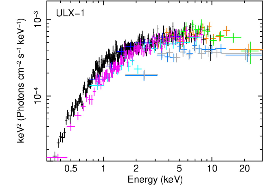
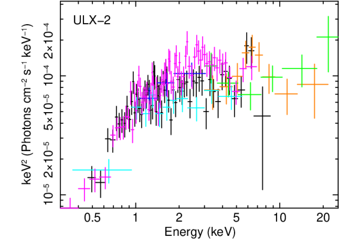
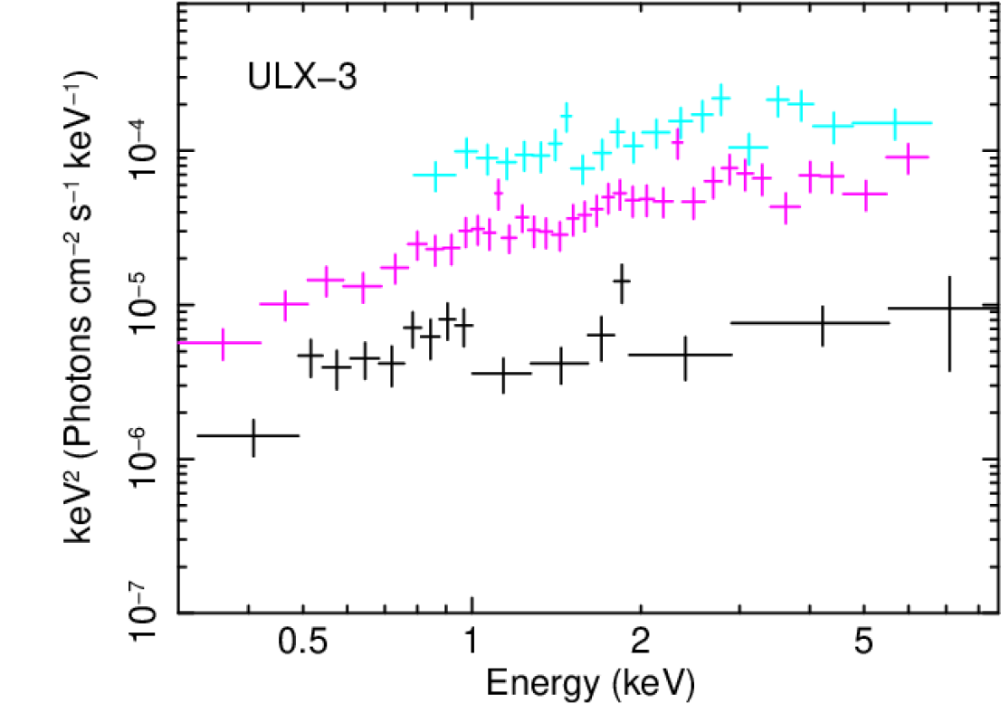
Figure 2: Unfolded spectra ($E^{2}f(E)$) for the three ULXs (data rebinned for display purposes) using a powerlaw model with photon index $\Gamma=0$. XMM-Newton EPIC-pn data are in black (for ULX-2 we plot instead the MOS1 data); NuSTAR FPMA 2017 (orange), NuSTAR FMPB 2017 (green); NuSTAR FPMA 2019 (grey); NuSTAR FMPB 2019 (light-blue); Chandra 7104 (blue); Chandra 20356 (cyan); Swift/XRT average (magenta).
Upper panel: ULX-1; Central panel: ULX-2; Bottom panel: ULX-3.

We carried out the spectral analysis by using xspec v.12.10.1 (Arnaud, 1996). We grouped the spectra from all the instruments with at least 20 counts per energy bin and we applied the $\chi^{2}$ statistics in the spectral analysis. In all the spectral fits, we included an absorbtion component modeled with tbabs and using the abundances of Lodders (2003).

Different models have been used in the literature to fit ULXs spectra, such as power-law, disc-like and comptonization continua (see e.g. Walton et al., 2013; Brightman et al., 2016; Pintore et al., 2016; Bachetti et al., 2013; Middleton et al., 2011; Roberts et al., 2006; Fürst et al., 2017).

ULXs spectra with low statistics (e.g. those obtained with Swift/XRT) can usually be fitted with simple models with one component. For high statistics data (e.g. XMM-Newton) instead, at least two components are needed to explain the complex spectral shape of ULXs (e.g. Gladstone et al., 2009; Pintore & Zampieri, 2011; Sutton et al., 2013; Middleton et al., 2015a; Walton et al., 2020). The need of two components models can be explained if we assume a regime of super-Eddington accretion onto a stellar mass compact object, where the disc is expected to be puffed up by the huge radiation pressure inside the spherization radius (see, e.g., Poutanen et al. 2007). A complex structure would likely arise implying the formation of zones with different temperatures and dominant radiation processes. In high counts X-ray spectra of ULXs, multiple components are often required in order to reproduce a hot, harder, inner accretion flow and a cooler, softer, outer disc component (see, e.g., Sutton et al. 2013). The hard component is commonly very broad with a strong turnover above 5 keV, while the soft component can be generally fitted with a simple black body or multi-colour black body disc. The latter component is usually referred as the outer disc and/or the photosphere of the optically thick outflows (see, e.g., Stobbart et al. 2006; Gladstone et al. 2009; Walton et al. 2020; Gúrpide et al. 2021a).

Motivated by the above-mentioned considerations on ULXs spectral-fitting, we first analysed the highest quality data, XMM-Newton + simultaneous (2017) NuSTAR data, for ULX-1 and ULX-2 and just XMM-Newton data for ULX-3, with two-component models. A good fit resulted from a two thermal components model for ULX-2 and ULX-3, i.e. a black body (bbodyrad in xspec) plus a multi-colour disc (diskbb; Mitsuda et al. 1984), while for ULX-1 a third harder spectral component, cutoffpl in xspec, was identified in the spectrum. The blackbody models the softer part of the spectra while the disc blackbody the harder part. We added also a multiplicative constant, const in xspec, to take into account different flux calibrations amongst instruments: all constants are consistent within 10%, as expected from e.g. Madsen et al. (2017).

For consistency, we applied the bbodyrad + diskbb model also to poorer statistics Chandra data and to the average Swift/XRT spectra. The absorbing column, composed of a fixed Galactic absorption (n${}_{H}^{gal}$ = 7.26$\times$10²⁰ cm^-2) plus an intrinsic absorption component, was not always well constrained, so we decided to fix it at the best value obtained with the XMM-Newton/NuSTAR (for ULX-2) data or XMM-Newton (for ULX-1, because the fit of the XMM-Newton / NuSTAR spectrum with two components was not statistically acceptable and in the fit with three components the n_H was not well constrained, and ULX-3, which was not detected in the NuSTAR data). The best-fitting spectral parameters are reported in Table 3. The unfolded spectra of each ULX are reported in Figure 2.

2.6 Hardness Ratio

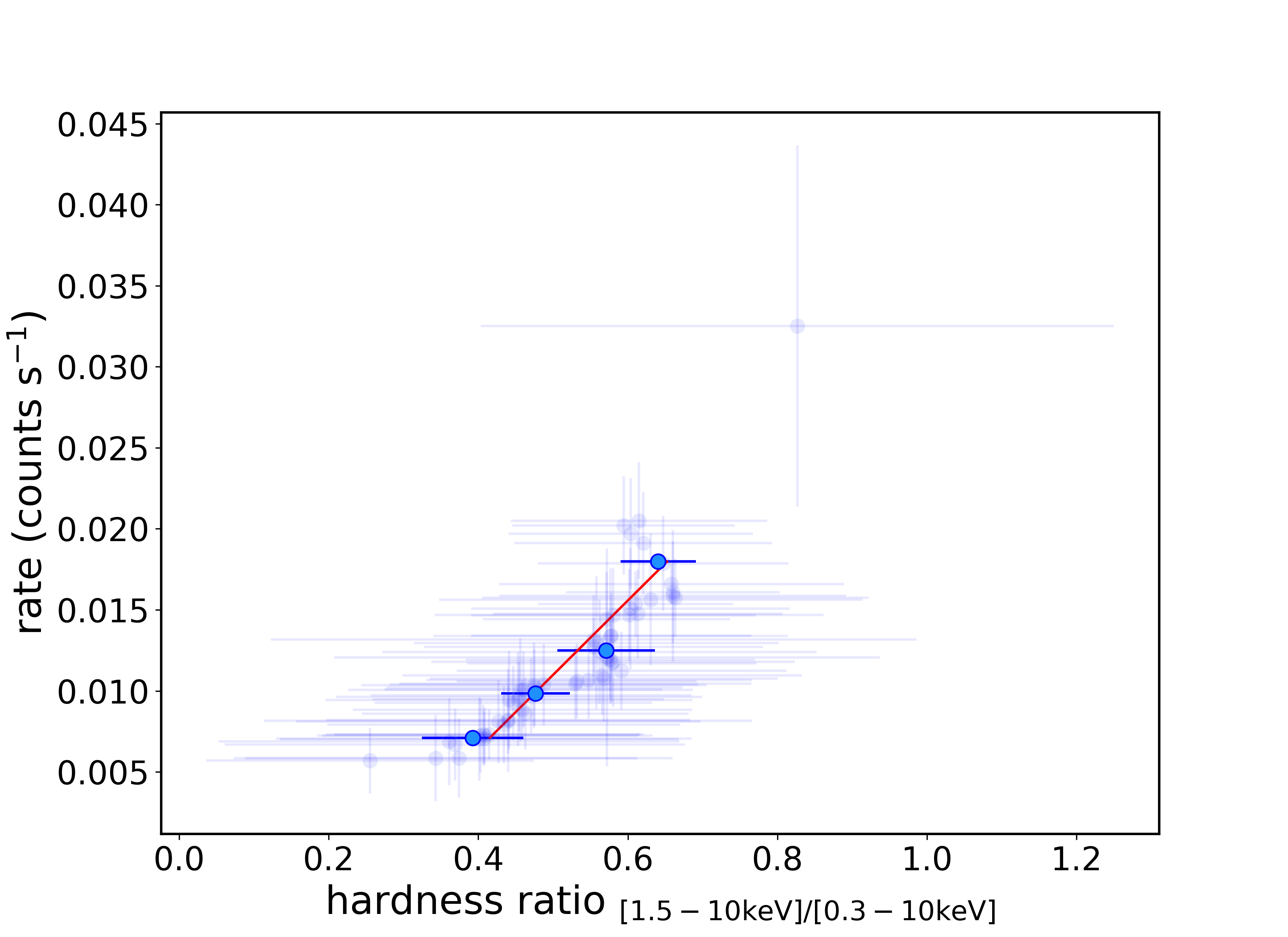
Figure 3: Swift/XRT count rate vs. hardness ratio for ULX-1 (upper); ULX-2 (middle); ULX-3 (bottom). The count rate is calculated in the (0.3-10 keV) band, in units of counts s^-1. The hardness ratio is the ratio between the count rates in (1.5-10) and (0.3-10) keV. The solid blue dots are the binned hardness ratios as a function of the count rate, while the transparent blue dots are the unbinned hardness ratios. The super-imposed solid line is the result of the linear regression applied to the binned points for: the hardness at low count rates ($<$ 0.04 cts s^-1) for ULX-1 (upper); all the binned points for ULX-2 (middle).

We derived a hardness–intensity diagram (HID) for each Swift/XRT observation, where the hardness was calculated as the ratio between the count rates in the hard (1.5-10 keV) and total (0.3-10 keV) energy bands, in each observation. We chose 1.5 keV as the threshold since it is about the median energy where the bbodyrad and diskbb spectral components cross for the three ULXs. Slight differences in this pivot energy are seen for the three sources, but we decided to adopt the same value for all the sources in order to allow a direct comparison of the results. The error bars of each point in the HID are large and did not permit us to identify clearly any trend or spectral evolution with the count rate. Therefore, in order to reduce data noise, we binned the hardness ratio based on the count rate. In particular, we grouped the data in order to have at least 15 observations in any given count rate bin for ULX-1 and ULX-2. Instead, for ULX-3, because of the lower statistics, we constructed bins containing at least 5 observations (see Figure  3).

From the HID, we note a possible linear trend for ULX-1 and ULX-2 at low count rates. We applied a linear fit to the binned data to verify it; we performed the fit applying the minimum least squares method. We report the results in sections 3.1 and 3.2.

2.7 Timing analysis

	soft[0.3-1.5]keV	hard[1.5-10.0]keV	total[0.3-10.0]keV
ULX-1	0.54$\pm$0.01	0.59$\pm$0.01	0.54$\pm$0.01
ULX-2	0.26$\pm$0.05	0.59$\pm$0.02	0.35$\pm$0.02
ULX-3	0.57$\pm$0.01	0.38$\pm$0.01	0.63$\pm$0.01

Table 4: ”Ensemble” fractional variability (F_var) for NGC 925 ULX-1, ULX-2, ULX-3. The reported uncertainties derive from the standard deviation of the distribution of the mean F_var: see text for more details.

We constructed the long-term Swift/XRT light-curves in the total energy band (0.3-10.0 keV) for each ULX and, for completeness, we added also the XMM-Newton and Chandra data (Fig. 4); the conversion factor between Swift/XRT count-rate and luminosity was obtained by the spectral fit of the average Swift/XRT spectrum with the black body plus multi-colour disc model. The Chandra and XMM-Newton luminosities have been derived from the spectral fit with the bbodyrad + diskbb model. We also plot in a separate panel of Fig. 4 the luminosity distribution for each ULXs, to look for any possible systematics, such as bi-modality. The Swift/XRT light-curves of all the sources are variable in flux on time-scales of at least days to weeks. We applied the Cash statistics (Cash, 1979) to verify at which significance the light-curves differ from a constant value. We also defined a flux variability factor for each ULX as the ratio of the highest to lowest flux. All these results are reported for each source in the next sections.

Figure 4: Light-curves, shown with six-day bins, and luminosity distributions of the three ULXs in NGC 925. The unabsorbed luminosity in the band [0.3-10] keV, in units of 10⁴⁰ erg s^-1, is derived from the best-fitting model in table 3. The Swift/XRT detections are marked with blue dots while the Swift/XRT upper limits with the black triangles; the XMM-Newton observation is marked with the red star; the Chandra data with the orange diamonds. Top: ULX-1. - Left, light-curve; right, histogram of the distribution of the Swift/XRT luminosity. Middle: ULX-2. - Left, light-curve; right, histogram of the distribution of the Swift/XRT luminosity. Bottom: ULX-3. - Left, light-curve (note that the X-axis scale is different from that used in the other panels); middle, histogram of the distribution of the Swift/XRT luminosity; right, histogram of the distribution of the Swift/XRT luminosity, with the upper limits superimposed in black.

A classical method to quantify the flux variability, used e.g. to study sparsely sampled light-curves of accreting objects, such as AGNs (e.g. Vagnetti et al. 2016; Aleksić et al. 2015; Schleicher et al. 2019), is the fractional variability amplitude (F_var; e.g. Vaughan et al. 2003; Edelson et al. 2002), which is defined as

$$F_{var}=\frac{1}{\langle X\rangle}\sqrt{S^{2}-\langle\sigma_{err}^{2}\rangle},$$ (1)

where S² is the total variance of the light-curve, $\langle\sigma_{err}^{2}\rangle$ is the mean error squared and $\langle X\rangle$ is the mean count rate. Here we use F_var to study the long-term variability of ULXs.

Allevato et al. (2013) demonstrated that the normalised excess variance evaluated from an individual light-curve, especially in case of irregularly sampled light-curves, might not be reliable. Thus, instead of deriving the estimate from the observed curve only, we used an “ensemble” approach, based on multiple simulated light-curves of the same source, as proposed in the cited paper. Since F_var is simply the square root of the normalised excess variance, we applied the method proposed in Allevato et al. (2013) to our case. We performed a simulation of 5000 light-curves, starting from the properties of the observed one. We derived the F_var applying the definition given in Equation 1 for each simulated light-curve and grouped the obtained values in bins of 50 points. We evaluated a mean F_var for each bin using Equation 12 in Allevato et al. (2013) and constructed the distribution of the obtained values. The estimates for F_var and its uncertainty are the mean of the distribution and its standard deviation. We report the obtained values in Table 4. We note that Allevato et al. (2013) also determine a bias on the variance estimate which depends both on the sampling pattern and on the power spectrum slope, if red noise is present in the data, as it may be in accreting compact objects (e.g. Vaughan et al. 2003). The red noise is characterised by a power spectrum with a power-law shape, with index 1–2 (e.g. Press 1978). If red noise were present in our data with a slope $\sim$ 2, the estimate of the fractional variability may reduce of $\sim$ 25%, while, for a slope $\sim$ 1, the effects coming from the irregular sampling pattern would dominate on the red noise and F_var may increase of $\sim$ 10%. The derivation of F_var does not take into account the upper limits. The effect of exclusion of significant upper limits is to underestimate F_var. Therefore, in such a case, the derived values have to be considered as lower limits on F_var. This happens mainly for ULX-3, where a number of significant upper limits is present in the light-curve, but not for ULX-1 and ULX-2, where the upper limits are rare.

We performed the simulations using a Monte Carlo approach. For each detection in the real light-curve, we extracted a random value from the normal distribution centered on the net (i.e. background-subtracted) detected count rate and standard deviation as large as the error on the count rate. We repeated the same procedure for the observed background count rate of each observation, normalised for the ratio of source and background extraction area. We then summed the two count rates and multiplied them by the exposure time, in order to obtain the total counts in the source region. From the total counts we derived the statistical uncertainty on the simulated rate, using the Gehrels approximation (Gehrels, 1986) when the total counts were less than 20, otherwise we used the square root of the counts.

We also looked for possible periodicities in the long-term light-curve of each source. We applied the Lomb-Scargle approach (Lomb 1976; Scargle 1982, see also VanderPlas 2018 for a recent review of the method) to derive the periodograms. We used the class LombScargle of the subpackage timeseries of the Python package for astronomy astropy. We found a periodicity only for ULX-3. To better constrain the result we followed the same Monte Carlo approach used for the determination of the fractional variability. In this case, we considered also the upper limits. For each upper limit in the real light-curve we generated a random number from a uniform distribution, from 0 to the upper limit value and the background rate as done in case of source detection. We applied the same procedure used for the detections to derive the uncertainty.

3 Results

3.1 ULX-1

ULX-1 is the most luminous of the three ULXs in NGC 925, with peak (unabsorbed) luminosity of $\sim$ 5$\times$10⁴⁰ erg s^-1 in the Swift/XRT data in 0.3-10 keV band. Its luminosity is in the range of the $\sim$ 10% most luminous ULXs presently known (e.g. Swartz et al. 2011; Walton et al. 2011; Earnshaw et al. 2019; Walton et al. 2021; Bernadich et al. 2021). The significance of its temporal variability is $\sim$ 37$\sigma$, calculated using the Cash statistics (Cash, 1979) on the timescale of $\sim$ 6 d – 10 yr. ULX-1 has a F_var of $\sim$ 54% in the total energy band and we estimated a flux variability as high as a factor of $\sim$ 8. The fit of the XMM-Newton / NuSTAR spectrum, modelled with the bbodyrad + diskbb model, leaves some residuals above 10 keV (see Figure 5 upper panel), suggesting the need for a third spectral component. A possibility is to add a cutoff power-law component (cutoffpl in xspec) as found in other ULXs (e.g. Walton et al. 2018b). We obtained kT_bbodyrad = 0.27${}^{+0.02}_{-0.02}$ keV, kT_diskbb = 1.3${}^{+0.6}_{-0.2}$ keV, $\Gamma$ = 0.1${}^{+0.6}_{-2.7}$ and HighECut = 5.2${}^{+1.9}_{-3.4}$ keV, with $\chi^{2}$/dof = 1288.3/1267. We fixed the n_H to the best-fitting value obtained by modelling XMM-Newton data only, because the more complex model did not allow us to constrain it. The residuals of the fit are shown in the bottom panel of Fig. 5. This additional spectral component describes well the spectrum above 10 keV, but other models are possible given the low statistics in the NuSTAR data. The Swift/XRT spectrum of the source is well described by a black body component with temperature kT${}_{bbodyrad}\sim$ 0.3 keV and a multi-colour disc with inner temperature of kT${}_{diskbb}\sim$ 2.1 keV.

The spectral parameters in the (0.3–10 keV) band found for the observations taken with the different satellites are consistent, despite the large flux variability, suggesting the absence of marked spectral variability.

From the HID (Figure 3-top), we note that there is no overall correlation. However, if we consider only the rates lower than 0.04 cts s^-1 (i.e. the three average bins at lower count rates), the linear fit gives a large correlation coefficient of 0.98. The regression model is plotted in Figure 3 (upper panel).

3.2 ULX-2

ULX-2 is the least variable in flux of the three ULXs and its peak luminosity (unabsorbed) in the Swift/XRT data is $\sim$ 1.5$\times$10⁴⁰ erg s^-1. The significance of its variability is $\sim$ 8$\sigma$ and the flux variability factor is $\sim$ 5. The fractional variability is dominated by the hard band (F${}_{var}\sim$59%). Instead, in the soft band the F_var results to be only $\sim$26% (see Table 4).

From the spectral analysis of the Swift/XRT stacked spectrum, we found that the bbodyrad temperature is $\sim$ 0.03 keV, but its normalization is not constrained, indicating that such a component is not significantly requested by the data. In fact, fitting the Swift/XRT average spectrum with a single diskbb, we found a fit statistics similar to that obtained with the two components model. The diskbb component temperature converges at $\sim$ 1.3 keV. Also the Chandra spectra can be modelled with a single component, while for the XMM-Newton data the diskbb does not provide a statistically acceptable fit, suggesting that the need for the two components arises only when the statistics is high. The spectral properties observed in the XMM-Newton / NuSTAR and Chandra spectral-fitting are consistent within 90% uncertainties, while those inferred in the Swift/XRT spectrum are different (kT${}_{diskbb}^{{\it XMM-Newton}\ /{\it NuSTAR}\ }$ = 1.9 keV vs kT${}_{diskbb}^{{\it Swift}/XRT\ }$ = 1.3 keV and (kT${}_{bbodyrad}^{{\it XMM-Newton}\ /{\it NuSTAR}\ }$ = 0.27 keV vs kT${}_{bbodyrad}^{{\it Swift}/XRT\ }$ = 0.03 keV), indicating a possible spectral variability for ULX-2.

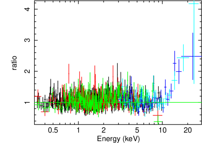
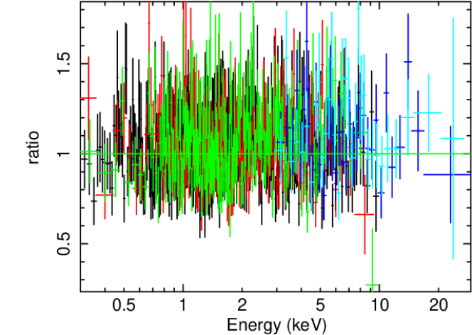
Figure 5: Upper: ULX-1 XMM-Newton EPIC pn(black), MOS1 (red), MOS2 (green), NuSTAR FPMA (blue), FPMB (cyan) residuals (data/model), for the bbodyrad + diskbb: an excess is clearly visible above 10 keV. Lower: ULX-1 residuals with the model bbodyrad + diskbb + cutoffpl, the colours are the same used in the upper panel.

We found that the Swift/XRT count rate of ULX-2 is always smaller than 0.04 cts s^-1 in the 0.3–10 keV band, and the hardness ratio shows evolution with the rate. In particular, we determined a linear trend by using the binned data (correlation factor $\sim$ 0.93), which indicates that the source becomes harder at the highest rates.

3.3 ULX-3

ULX-3 is a transient ULX with hints of (super-)orbital periodicity (Earnshaw et al., 2020). According to the Swift/XRT long-term monitoring, its unabsorbed luminosity reaches a peak of $\sim$ 1.5$\times$10⁴⁰ erg s^-1, its variability significance is $\sim$22$\sigma$ and its flux variability factor is $\sim$ 7. However, the latter is only a lower limit because of the presence of many upper limits in its long-term light-curve: indeed, considering also the lowest Chandra upper-limit, Earnshaw et al. (2020) found a factor of variability up to $\sim$ 30.

The $F_{var}$ of ULX-3 is $\sim$ 63% in the total 0.3–10 keV energy band. The highest amount of variability is seen in the soft band ($<1.5$ keV) unlike what is usually found in ULXs, for which the hard band is generally the most variable, at least on short timescales (e.g. Sutton et al., 2013; Pintore et al., 2020). However, such a behaviour is possibly due to the fact that here the spectral shape changes around 1 keV. Therefore, we repeated the estimate of the variability dividing the bands at 1 keV. In this case we found a larger value for F_var in the hard energy band ($\sim$54%), while in the soft band the variability is $\sim$40%. This implies that the highest variability concentrates around 1-2 keV.

We analysed the average Swift/XRT spectrum of ULX-3 with the same model used for the other ULXs (i.e. bbodyrad + diskbb in xspec), obtaining a cool black body (kT${}_{bbodyrad}\sim$ 0.1 keV) and a diskbb with a temperature of $\sim$1.5 keV.

The hardness ratio of ULX-3 is consistent with a constant within the uncertainties, with a mean value of $\sim$ 0.5 at the detected count rates.

We applied the Lomb-Scargle method to the ULX-3 light-curve to search for periodic variability. We used only the Swift/XRT observations, stacked in time bins of $\sim$ 6 d, taken between 2019 and March 2021 (i.e. MJD ¿ 58500), where the monitoring was denser and more regular. This allowed us to exclude periods of long-term gaps where the behaviour of the source was unknown (for example it could have faded).

We applied the Lomb-Scargle approach to the frequency range [2$\times$10^-3 – 0.08] d^-1, which corresponds to the period range 12–500 d. At first, we used only the Swift/XRT data with a source detection. We found several peaks in the power density spectrum, the most prominent of which corresponds to a period of $\sim$ 126 d. However, the peak was not statistically significant because of the sparse distribution of the data. Thus we decided to include also the information carried by the significant upper limits (UL), to reduce the gaps between the observations. We included them somewhat arbitrarily at half the value of each UL with an associated uncertainty of the same amount. The new Lomb-Scargle power spectra is showed in Fig. 6. The peak at the period of 126 d is now predominant.

To assess the goodness of our approach, we performed a Monte-Carlo simulation (see section 2.7 for details) of 5000 light-curves considering both detections and upper limits, between 2019 and March 2021, in the original light-curve showed in Fig. 4-lower panel. In the simulations, the value corresponding to each upper limit is derived from a random value in the uniform distribution between zero and the upper limit value, considering each value equally probable. For each simulated light-curve we applied a Lomb–Scargle analysis. We constructed the histogram of the highest peak frequencies obtained from the simulated light-curves and we fit such a distribution with a Gaussian function. We found that the mean value and the standard deviation of the Gaussian are 126.1 d and 2.0 d, respectively. The best-period is therefore totally compatible with the one we found using only the Swift/XRT detections. Therefore we claim the existence of a periodicity of $126\pm 2$ d. A superposition of the expected periodicity on the observed data is shown in Fig. 7. If we extrapolate the detected periodicity to the data taken before 2019, we find that the curve does not follow the observations. This could indicate that either the periodicity has slightly changed or its phase has shifted in time, or it could depend on the uncertainties on the highest peak (see figure 7). A better superposition of the same periodicity on the older points is found with a shift in phase of $\sim$ 55 days in about 10 years, although the number of points is small: similar shifts have been observed in the super-orbital periodicity of other ULXs, see for example Brightman et al. (2019).

The significance of the peak corresponding to the best period has been determined with the Baluev method (Baluev, 2008), an analytical approximation to determine the false alarm probability (FAP), i.e. the probability to obtain a peak equal or higher than the considered one if only noise is present. From the observed light-curve, we obtained a FAP value of $\sim$ 10^-8, which should be considered as an upper limit. Therefore the significance of the peak should be $>$5$\sigma$. We must notice that the determination of the peak significance through the FAP assumes white noise (the height of spurious peaks is independent from frequency; VanderPlas 2018). This assumption could be not true for compact accreting objects, which may present red noise (Vaughan et al., 2003). To take into account this effect, we used an approach similar to that followed by Walton et al. (2016) for NGC 5907 ULX-1. We simulated 5000 light-curves with a red noise power spectrum, assuming a power-law with slope 1 and 2. We performed the simulations using the Simulator object of the Python library for spectral timing Stingray v.0.2, which applies the algorithm from Timmer & Koenig (1995) (see Huppenkothen et al. 2019b and Huppenkothen et al. 2019a for a description of the library). We simulated continuous light-curves, with a time resolution of 2 ks, and we selected only time bins corresponding to the epochs of the real data. For each simulated curve, we ran the Lomb–Scargle method to look for peaks comparable to the real data one but generated by random noise. In the worst case, i.e. slope=2, we found that most of the peaks generated from the random noise have frequencies smaller than 0.0035 1/d (280 d), which corresponds to roughly half of our observing window. Therefore peaks corresponding to longer periods (i.e. smaller frequencies) are about the 70% of the total number of peaks. However, these peaks are not reliable because they would cover less than 2 cycles in the light-curve time window. Only two-three peaks have a period comparable or smaller and a significance larger than that of the real peak from the observed light-curve. These correspond to $\sim$ 0.05% of the total number of peaks derived from the red noise simulations. Therefore the significance of the periodicity detection may decrease to $\sim$ 3.4$\sigma$ in the worst case of possible red noise. For a slope=1, only two peaks in the total frequency band have significance larger than our period detection, both of them at significantly smaller frequencies than that of the periodicity. So, even if red noise were present, it is unlikely that the peak corresponding to the period in the real data has been generated by chance from the random noise.

We also wanted to verify if a short-term pulsation period, such as those found in the PULX, was present. So we searched for coherent signals in ULX-3 XMM-Newton data also including the correction for a possible first period derivative component (1$\times$10${}^{-6}<\left|P_{dot}/P\right|<1\times$10^-12) but no significant signals were detected. The 3$\sigma$ upper limits on the fractional amplitude (defined as the semi-amplitude of the sinusoid divided by the average source count rate) are between 70% $-$ 100% in the period range 500$-$0.150s

4 Discussion

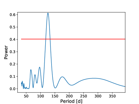
Figure 6: (Super-)orbital period in NGC 925 ULX-3. Power vs. frequency, from the Lomb-Scargle periodogram. The level corresponding to 3$\sigma$ significance is indicated by the red line.

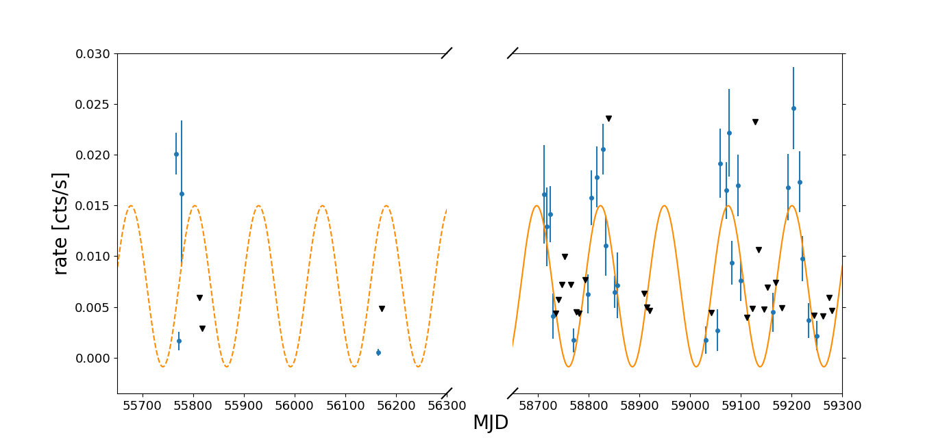
Figure 7: (Super-)orbital period in NGC 925 ULX-3. Light-curve binned in interval of 6 days of NGC ULX-3 with the sinusoidal best-fitting of the periodicity superimposed. The period has been estimated on the more recent and denser data (solid orange line) and has been extrapolated to the older data (dashed orange line). The blue dots are the Swift/XRT detections, while the black inverted triangles are upper limits.

We have studied the timing and spectral properties of the three ULXs in the galaxy NGC 925, analysing all the available Swift/XRT, XMM-Newton, Chandra and NuSTAR public observations. In the following, we discuss the main results of this manuscript and their implications for the detected ULXs.

4.1 Temporal variability

The three ULXs in NGC 925 are confirmed to be all variable in flux on days-to-weeks timescales. The fractional variability has been often used to study the variability properties of ULXs within individual observations, typically considering timescales of minutes – hours (e.g. Sutton et al. 2013; Pintore et al. 2020; Mondal et al. 2021; Robba et al. 2021). Here, we used this estimator on longer timescales (using 6 days bins), applying it to sparse sampled light-curves, using the ‘ensemble’ approach proposed in Allevato et al. (2013), as explained in section 2.7.

The most luminous of the ULXs in NGC 925 is ULX-1, which alternated epochs of ”high-flux” (0.3-10 keV $F_{abs}>3\times 10^{-12}$ erg s^-1 cm^-2 ) in some of the observations taken in 2011, and ”low-flux” (0.3-10 keV $F_{abs}<3\times$10^-12 erg s^-1 cm^-2) in the subsequent observations. However, from February 2021 the source entered again in a high flux regime, from which it dropped on 8 March 2021, the last observation before a period of non-visibility for the Swift satellite that was monitoring the galaxy. It has a large F_var, with a value of $\sim$54% in the total energy band. Similarly, ULX-3 was also highly variable (F${}_{var}\sim 60\%$) on weekly timescales.

ULX-2 is the least variable of the three ULXs, with a variability amplitude of $\sim$ 35% in the total band. The variability is driven by the high energy component, with $F_{var}$ $>50\%$, while the soft band variability is just 20-30%. This trend is also present in the other two ULXs, even if it is less pronounced. This behaviour is consistent with the results of previous works which analysed other ULXs variability on smaller time-scales (e.g. Middleton et al., 2015b; Walton et al., 2018a).

The transient ULX-3 is the only one of the three ULXs in NGC 925 to show a candidate (super-)orbital periodicity. From the Lomb-Scargle method, we estimated a periodicity consistent with the interval of 70-150 days previously found by Earnshaw et al. (2020). In particular, we found that, during the Swift/XRT monitoring campaign which started in 2019, the source presents a periodicity of $\sim 126$ d, which we proved to be significant. The observations used cover only four cycles of the inferred periodicity, and we found that an extrapolation of it at earlier epochs is not consistent with the data. Either the source experienced a period of turn-off of the accretion during the epochs where it was not monitored, or the phase of the periodicity may have changed for other effects as the onset of a propeller regime or a change in the geometrical configuration of the accretion system. Further coverage of the source should give better constraints.

Periodicities of the order of tens/hundreds of days discovered from the flux variability in ULX light-curves are often interpreted as super-orbital variabilities (e.g. Israel et al. 2017a, Brightman et al. 2019) and may be linked to some kind of precession, e.g. of a warped accretion disc, of a large height disc or a Lense-Thirring precession, as has been found in many binaries (e.g. Motch et al. 2014; Hu et al. 2017; Fürst et al. 2017; Middleton et al. 2018).

Long-term light-curves of ULXs can be used to search for possible propeller phases (e.g. Earnshaw et al. 2018; Song et al. 2020), indicating the presence of a NS accretor. Given that, during a propeller phase, the accretion on the compact object is expected to stop, the presence of a flux bi-modal distribution with orders of magnitude difference, corresponding to active and non-active periods of accretion, identifies PULX candidates. Despite its large flux variability, there are no indications of propeller phases in the light-curve of ULX-1: the histogram of the luminosity (figure 4, upper panel - right) does not indicate a bi-modal distribution. Furthermore, Lara-López et al. 2021 found a low-metallicity environment around ULX-1, which in principle could favour the formation of BHs with respect to NSs, since less mass loss is expected in low-metallicity stars (e.g. Heger et al. 2003). In contrast, the excess found in the residuals above 10 keV in the NuSTAR data may be explained with the emission of the accreting column above the magnetic poles of a NS, as seen in other ULXs (e.g. Walton et al. 2018b). Also for ULX-2 the luminosity is always larger than 10³⁹ erg s^-1 and no bi-modal flux distribution is observed in the light-curve. ULX-3 is the only ULX in NGC 925 with many upper limits. Between MJD 56165 and 57770 (about 4 years) the source has been observed only twice with Swift/XRT, without detections, before the one with XMM-Newton (MJD 57771). We cannot exclude that in this period the source flux could have decreased by a large amount, because of a propeller phase, but the upper limits found are also compatible with the lower fluxes of the (super-)orbital modulation. Lara-López et al. (2021) found high-metallicity around ULX-3, consistent with the possibility that the compact object may be a NS. The confirmation of the presence of a NS would come from the detection of pulsations, but the low statistics of the XMM-Newton data allowed us to just derive an upper limit on the fractional amplitude (see section 3.3). Only upper limits have been found also for the pulsation period in ULX-1 and ULX-2 (see Pintore et al. 2018b for details).

4.2 Spectral classification

Following the classification described in Sutton et al. (2013) and using the 2017 XMM-Newton data, we classified the spectral regime of the three ULXs (see also section 1 for details on the classification method).

ULX-1 was spectrally stable in all the available data and, according to the best-fitting diskbb+powerlaw model ($\Gamma\sim$ 1.8, T${}_{diskbb}\sim$ 0.2), ULX-1 can be classified as a hard ultraluminous source (HUL). However, considering also the NuSTAR data the model leaves an excess at high energies, suggesting a spectral curvature (as found by Pintore et al. 2018b), which resembles the spectral shape of a broadened disc (BD). Sutton et al. (2013) highlighted the difficulty to distinguish the HUL regime from the BD one, for sources with a pronounced curvature, perhaps caused by a strong comptonization. In order to model the high energy spectral curvature we fit the XMM-Newton+NuSTAR spectrum of ULX-1 with a multi-colour disc (MCD) plus a high energy cutoff power-law (highecut$\times$powerlaw, in xspec). The $\Gamma$ and kT values we found are consistent with the ones from the previous fit with XMM-Newton data only, confirming the classification as an HUL source for ULX-1. Similar results were also confirmed by the Swift/XRT average spectrum. This indicates that, despite the flux variability, there is no evident spectral variability over the considered period. The HID of ULX-1 confirms that it is a rather hard source. Pintore et al. (2018b) proposed that the hard emission from ULX-1 could be explained by a system seen at a small inclination angle (nearly face-on), where, in a scenario of super-Eddington accretion onto a stellar mass compact object, the hard emission from the innermost regions of the accretion flow is not covered by the outflows. They also studied the hardness ratio for NGC 925 ULX-1, using a colour-colour diagram, in the energy band 2-30 keV and found that the position of ULX-1 was close to that of the PULXs analysed in Pintore et al. (2017). With the available data analysed here, we could not determine the nature of the compact object in ULX-1, which remains still unknown.

The fit of the simultaneous XMM-Newton+NuSTAR spectra of ULX-2 with a multi-colour disc plus a power-law (kT=0.2 keV and $\Gamma$=1.9) allowed us to classify ULX-2 as likely a hard Ultraluminous (HUL) source. However, if we take into account the uncertainties on $\Gamma$, which can vary between 1.7 and 2.1, the source could be a SUL ULX as well. As pointed out by Sutton et al. (2013), both regimes can take place in the same system, depending on changes in the accretion rate and in the wind’s opening angle, which has the shape of a funnel (as resulted from the simulations of Kawashima et al. 2012). So we suggest that ULX-2 is seen at intermediate inclination angles (between face-on direction, where the hard emission from the inner regions would be predominant, and the funnel inclination angle direction, where we would see the softer emission of the wind’s photosphere) appearing in a SUL/HUL regime. We found a linear correlation, with the source becoming harder at larger count rates, in the HID of ULX-2. This could be interpreted with a source seen at small inclination angles, nearer to the face-on position than to the edge-on one, leaving the inner regions of the accretion flow, which become brighter and hotter with increasing rates, directly visible to the observer. An alternative explanation is linked to the beaming. While the count rate increases, due to an enhancement in the mass accretion rate ($\dot{m}$), the wind opening angle narrows. The hard emission becomes consequently more beamed. Therefore both the hard and soft emission increase, but the beamed hard emission increase is proportional to $\dot{m}^{2}$ (King 2009), while the soft one to $\dot{m}$, resulting in an overall hardening (see e.g. Middleton et al. 2015a). This mechanism has been proposed by Luangtip et al. (2016) to explain the source Ho IX X-1, where it was also observed a shift of the peak in the hard component towards lower temperatures, while the luminosity increases. The authors explained this considering the simulated spectra for comptonising BHs (Kawashima et al. 2012), which appear to be harder at lower super-Eddington rates, because of photon up-scattering in the shocked region near the BH and softer at extreme super-critical rates, when the wind funnel narrows reducing the number of photons which can escape without intercepting the wind and being Compton down-scattered.

For ULX-3 we found a cool disc temperature ($\sim$ 0.09 keV) and a photon index between $\sim$ 1.7 and 3.2, so in this ULX may be present both the HUL and SUL regimes. The average Swift/XRT spectrum (magenta in the lower panel of figure 2) of ULX-3, which is more luminous than the XMM-Newton one, has also a harder spectral shape, with best-fitting values kT${}_{diskbb}\sim$ 0.09 keV and $\Gamma\sim$ 1.6. From this data ULX-3 can be classified as a hard ultraluminous ULX. This trend is in accordance with the result of Earnshaw et al. (2020), who found a softer spectrum at low luminosities which became harder at higher ones. As already noted by Earnshaw et al. (2020), this behaviour could indicate a propeller effect causing a soft and dim state in the absence of accretion onto the compact object, but the flux observed in the XMM-Newton observation is still compatible with the periodic flux modulation. In contrast, the hardness ratio seems constant among the observed count rates, within the errors.

Considering the known PULXs, they are usually found in the hard ultraluminous regime (e.g. Sutton et al. 2013; Pintore et al. 2017; Carpano et al. 2018). The disc temperatures of the ULXs in NGC 925 are similar to those observed in the PULXs ($\sim$ 0.04 – 0.2 keV), while the power-law index of the PULXs ($\Gamma\sim 1-1.9$) are sometimes comparable to and other times harder than the sources analysed in this work.

4.3 Super-Eddington accretion

From the normalizations of the fitting components, it is possible to derive the apparent emitting radii for the bbodyrad and diskbb components. We remark that such dimensions might not have a real physical meaning but they allow us to give a first, tentative characterisation of the accretion geometry.

From the Swift/XRT average spectrum of ULX-1, the radii of the bbodyrad and diskbb are 1452${}^{+588}_{-362}$ km and 75${}^{+14}_{-17}$ km respectively (assuming a reference inclination angle of 45^∘). Such values are similar to those observed in a number of ULXs (e.g. 4X J1118, Motta et al. 2020; Circinus ULX-5, Mondal et al. 2021; Walton et al. 2020). Considering that the source is in an ultraluminous accretion regime, we expect the accretion disc to be supercritical, with advection (slim disc model) and outflows (e.g. Shakura & Sunyaev 1973; Poutanen et al. 2007). The disc is expected to be geometrically thick inside the spherisation radius, where a fraction of the accreting matter is radiatively expelled from the disc in the form of a powerful wind, and geometrically thin in the very outer regions. The latter can be cold and not contribute much to the total ULX flux. In addition, the inner regions of the accretion flow may be also naked, i.e. the outflows are no more present above the thick disc. As proposed by some authors (e.g. Walton et al. 2015b; Pintore et al. 2018b), in this scenario the larger radius could be interpreted as an average size of the region where the winds are launched, while the smaller radius may be the size of the inner disc. Assuming accretion onto a non-rotating BH, the inner disc radius (R_in) would be three times the Schwarzschild radius, i.e. R_in = 6 GM / c². The apparent inner disc dimension of $\sim 75$ km is too small to be the inner disc radius of an IMBH (which would result larger than $\sim 900$ km, assuming a minimum mass of 100M_⊙), but also of a massive stellar mass BH (30–100 M_⊙), suggesting that the ULX may host a lighter stellar mass BH (M${}_{BH}<$ 10M_⊙) or a NS.

The radius of the hot component derived from the Swift/XRT average spectrum for ULX-2 is 89${}^{+12}_{-14}$ km (for an inclination angle of 45^∘). This value is consistent with that found by Pintore et al. (2018b) from the XMM-Newton / NuSTAR data and the considerations for ULX-1 hold for ULX-2 also, i.e. the internal disc radius may correspond to that of a light BH or a NS.

In the case of ULX-3, the radius associated with the colder emitting region is 7200${}^{+6100}_{-3000}$ km, while the hotter emitting region has a radius R_diskbb = 47${}^{+11}_{-14}$ km for a 45^∘ inclination angle. The last one, if corresponding to the inner disc radius of an accreting compact object, would belong to a compact object mass even smaller than in the case of ULX-1 and ULX-2.

5 Conclusion

All the three ULXs analysed in this work are variable on time-scales of days/months. One of them, ULX-3, has a candidate (super-)orbital periodicity on a time-scale of months ($\sim$ 126 d) similar to the super-orbital periodicities observed in some other ULXs.

The spectral study of all the three sources suggests that they are all in a super-Eddington accretion regime, the hard ultraluminous regime for ULX-1 and an intermediate situation between the hard and soft ultraluminous regime for ULX-2 and ULX-3, for which a unique classification is not possible, indicating that repeated observations are necessary to investigate fully the emission of ULXs. While ULX-1 shows only weak spectral variability, for the other two sources we found hints of a significant spectral variability. The spectral-timing properties suggest that ULX-1 and ULX-2 are being seen close to face-on, while ULX-3 may be seen through the wind in a super-Eddington scenario.

Follow-up observations would be useful to double check the periodicities and place stronger constraints on the pulsed fraction.

6 Acknowledgements

This work has been partially supported by the ASI-INAF program I/004/11/4 and the ASI-INAF agreement n.2017-14-H.0. EA acknowledges funding from the Italian Space Agency, contract ASI/INAF n. I/004/11/4. We acknowledge the usage of the HyperLeda database (http://leda.univ-lyon1.fr). This work made use of the data from the UK Swift Science Data Centre (University of Leicester) and of the XRT Data Analysis Software (XRTDAS) developed by the ASI Science Data Center (Italy).

7 Data availability

The Swift, XMM-Newton, Chandra and NuSTAR data used in this work are available respectively from https://www.swift.ac.uk/swift_portal/, https://www.cosmos.esa.int/web/xmm-newton/xsa, https://cxc.harvard.edu/cda/ and https://heasarc.gsfc.nasa.gov/.

References

- Aleksić et al. (2015) Aleksić J., et al., 2015, A&A, 576, A126
- Allevato et al. (2013) Allevato V., Paolillo M., Papadakis I., Pinto C., 2013, ApJ, 771, 9
- Alston et al. (2021) Alston W. N., et al., 2021, arXiv e-prints, p. arXiv:2104.11163
- An et al. (2016) An T., Lu X.-L., Wang J.-Y., 2016, A&A, 585, A89
- Arnaud (1996) Arnaud K. A., 1996, in Jacoby G. H., Barnes J., eds, Astronomical Society of the Pacific Conference Series Vol. 101, Astronomical Data Analysis Software and Systems V. p. 17
- Bachetti et al. (2013) Bachetti M., et al., 2013, ApJ, 778, 163
- Bachetti et al. (2014) Bachetti M., et al., 2014, Nature, 514, 202
- Bachetti et al. (2020) Bachetti M., et al., 2020, StingraySoftware/stingray: Version 0.2, doi:10.5281/zenodo.3898435, https://doi.org/10.5281/zenodo.3898435
- Baluev (2008) Baluev R. V., 2008, MNRAS, 385, 1279
- Belfiore et al. (2020) Belfiore A., Esposito P., Pintore F., Novara G., et al., 2020, Nature Astronomy, 4, 147
- Bernadich et al. (2021) Bernadich M. C. i., Schwope A. D., Kovlakas K., Zezas A., Traulsen I., 2021, arXiv e-prints, p. arXiv:2110.14562
- Brightman et al. (2016) Brightman M., et al., 2016, ApJ, 829, 28
- Brightman et al. (2018) Brightman M., et al., 2018, Nature Astronomy, 2, 312
- Brightman et al. (2019) Brightman M., et al., 2019, ApJ, 873, 115
- Brightman et al. (2020) Brightman M., et al., 2020, ApJ, 895, 127
- Carpano et al. (2018) Carpano S., Haberl F., Maitra C., Vasilopoulos G., 2018, MNRAS, 476, L45
- Cash (1979) Cash W., 1979, ApJ, 228, 939
- Colbert & Mushotzky (1999) Colbert E. J. M., Mushotzky R. F., 1999, ApJ, 519, 89
- Cseh et al. (2012) Cseh D., et al., 2012, ApJ, 749, 17
- D’Aì et al. (2021) D’Aì A., et al., 2021, MNRAS, 507, 5567
- Earnshaw et al. (2018) Earnshaw H. P., Roberts T. P., Sathyaprakash R., 2018, MNRAS, 476, 4272
- Earnshaw et al. (2019) Earnshaw H. P., Roberts T. P., Middleton M. J., Walton D. J., Mateos S., 2019, MNRAS, 483, 5554
- Earnshaw et al. (2020) Earnshaw H. P., et al., 2020, ApJ, 891, 153
- Ebisuzaki et al. (2001) Ebisuzaki T., et al., 2001, ApJ, 562, L19
- Edelson et al. (2002) Edelson R., Turner T. J., Pounds K., Vaughan S., Markowitz A., Marshall H., Dobbie P., Warwick R., 2002, ApJ, 568, 610
- Evans et al. (2009) Evans P. A., et al., 2009, MNRAS, 397, 1177
- Farrell et al. (2009) Farrell S. A., Webb N. A., Barret D., Godet O., Rodrigues J. M., 2009, Nature, 460, 73
- Feng et al. (2016) Feng H., Tao L., Kaaret P., Grisé F., 2016, ApJ, 831, 117
- Foster et al. (2010) Foster D. L., Charles P. A., Holley-Bockelmann K., 2010, ApJ, 725, 2480
- Fruscione et al. (2006) Fruscione A., et al., 2006, in Proc. SPIE. p. 62701V, doi:10.1117/12.671760
- Fürst et al. (2016) Fürst F., et al., 2016, ApJ, 831, L14
- Fürst et al. (2017) Fürst F., Walton D. J., Stern D., Bachetti M., Barret D., Brightman M., Harrison F. A., Rana V., 2017, ApJ, 834, 77
- Fürst et al. (2018) Fürst F., et al., 2018, A&A, 616, A186
- Gehrels (1986) Gehrels N., 1986, ApJ, 303, 336
- Gehrels et al. (2004) Gehrels N., Chincarini G., Giommi P., Mason K. O., Nousek J. A., et al., 2004, ApJ, 611, 1005
- Gladstone et al. (2009) Gladstone J. C., Roberts T. P., Done C., 2009, MNRAS, 397, 1836
- Grebenev (2017) Grebenev S. A., 2017, Astronomy Letters, 43, 464
- Grisé et al. (2010) Grisé F., Kaaret P., Feng H., Kajava J. J. E., Farrell S. A., 2010, ApJ, 724, L148
- Gúrpide et al. (2021a) Gúrpide A., Godet O., Koliopanos F., Webb N., Olive J. F., 2021a, A&A, 649, A104
- Gúrpide et al. (2021b) Gúrpide A., Godet O., Vasilopoulos G., Webb N. A., Olive J. F., 2021b, A&A, 654, A10
- Heger et al. (2003) Heger A., Fryer C. L., Woosley S. E., Langer N., Hartmann D. H., 2003, ApJ, 591, 288
- Heil et al. (2009) Heil L. M., Vaughan S., Roberts T. P., 2009, MNRAS, 397, 1061
- Hu et al. (2017) Hu C.-P., Li K. L., Kong A. K. H., Ng C. Y., Lin L. C.-C., 2017, ApJ, 835, L9
- Huppenkothen et al. (2019a) Huppenkothen D., et al., 2019a, Journal of Open Source Software, 4, 1393
- Huppenkothen et al. (2019b) Huppenkothen D., et al., 2019b, ApJ, 881, 39
- Illarionov & Sunyaev (1975) Illarionov A. F., Sunyaev R. A., 1975, A&A, 39, 185
- Israel et al. (2017a) Israel G. L., et al., 2017a, Science, 355, 817
- Israel et al. (2017b) Israel G. L., et al., 2017b, MNRAS, 466, L48
- Kaaret & Feng (2009) Kaaret P., Feng H., 2009, ApJ, 702, 1679
- Kaaret et al. (2017) Kaaret P., Feng H., Roberts T. P., 2017, ARA&A, 55, 303
- Kawashima et al. (2012) Kawashima T., Ohsuga K., Mineshige S., Yoshida T., Heinzeller D., Matsumoto R., 2012, ApJ, 752, 18
- King (2009) King A. R., 2009, MNRAS, 393, L41
- Koliopanos et al. (2017) Koliopanos F., Vasilopoulos G., Godet O., Bachetti M., Webb N. A., Barret D., 2017, A&A, 608, A47
- Kosec et al. (2018) Kosec P., Pinto C., Walton D. J., et al., 2018, MNRAS, 479, 3978
- La Parola et al. (2015) La Parola V., D’Aí A., Cusumano G., Mineo T., 2015, A&A, 580, A71
- Lara-López et al. (2021) Lara-López M. A., et al., 2021, ApJ, 906, 42
- Lodders (2003) Lodders K., 2003, ApJ, 591, 1220
- Lomb (1976) Lomb N. R., 1976, Ap&SS, 39, 447
- Luangtip et al. (2016) Luangtip W., Roberts T. P., Done C., 2016, MNRAS, 460, 4417
- Madsen et al. (2017) Madsen K. K., Beardmore A. P., Forster K., Guainazzi M., Marshall H. L., Miller E. D., Page K. L., Stuhlinger M., 2017, AJ, 153, 2
- Makarov et al. (2014) Makarov D., Prugniel P., Terekhova N., Courtois H., Vauglin I., 2014, A&A, 570, A13
- Middleton et al. (2011) Middleton M. J., Sutton A. D., Roberts T. P., 2011, MNRAS, 417, 464
- Middleton et al. (2015a) Middleton M. J., Heil L., Pintore F., Walton D. J., Roberts T. P., 2015a, MNRAS, 447, 3243
- Middleton et al. (2015b) Middleton M. J., Walton D. J., Fabian A., Roberts T. P., Heil L., Pinto C., Anderson G., Sutton A., 2015b, MNRAS, 454, 3134
- Middleton et al. (2018) Middleton M. J., et al., 2018, MNRAS, 475, 154
- Mitsuda et al. (1984) Mitsuda K., et al., 1984, PASJ, 36, 741
- Mondal et al. (2021) Mondal S., Rozanska A., Baginska P., Markowitz A., De Marco B., 2021, arXiv e-prints, p. arXiv:2104.12894
- Motch et al. (2014) Motch C., Pakull M. W., Soria R., Grisé F., Pietrzyński G., 2014, Nature, 514, 198
- Motta et al. (2020) Motta S. E., et al., 2020, ApJ, 898, 174
- Pakull et al. (2010) Pakull M. W., Soria R., Motch C., 2010, Nature, 466, 209
- Pinto et al. (2016) Pinto C., Middleton M. J., Fabian A. C., 2016, Nature, 533, 64
- Pinto et al. (2017) Pinto C., Alston W., Soria R., Middleton M. J., Walton D. J., et al., 2017, MNRAS, 468, 2865
- Pinto et al. (2021) Pinto C., et al., 2021, MNRAS, 505, 5058
- Pintore & Zampieri (2011) Pintore F., Zampieri L., 2011, Astronomische Nachrichten, 332, 337
- Pintore et al. (2014) Pintore F., Zampieri L., Wolter A., Belloni T., 2014, MNRAS, 439, 3461
- Pintore et al. (2016) Pintore F., Zampieri L., Sutton A. D., Roberts T. P., Middleton M. J., Gladstone J. C., 2016, MNRAS, 459, 455
- Pintore et al. (2017) Pintore F., Zampieri L., Stella L., Wolter A., Mereghetti S., Israel G. L., 2017, ApJ, 836, 113
- Pintore et al. (2018a) Pintore F., et al., 2018a, MNRAS, 477, L90
- Pintore et al. (2018b) Pintore F., et al., 2018b, MNRAS, 479, 4271
- Pintore et al. (2020) Pintore F., et al., 2020, ApJ, 890, 166
- Pintore et al. (2021) Pintore F., et al., 2021, MNRAS, 504, 551
- Poutanen et al. (2007) Poutanen J., Lipunova G., Fabrika S., Butkevich A. G., Abolmasov P., 2007, MNRAS, 377, 1187
- Press (1978) Press W. H., 1978, Comments on Astrophysics, 7, 103
- Robba et al. (2021) Robba A., et al., 2021, A&A, 652, A118
- Roberts (2007) Roberts T. P., 2007, Ap&SS, 311, 203
- Roberts et al. (2006) Roberts T. P., Kilgard R. E., Warwick R. S., Goad M. R., Ward M. J., 2006, MNRAS, 371, 1877
- Rodríguez Castillo et al. (2019) Rodríguez Castillo G. A., et al., 2019, arXiv e-prints, p. arXiv:1906.04791
- Sathyaprakash et al. (2019) Sathyaprakash R., et al., 2019, MNRAS, 488, L35
- Scargle (1982) Scargle J. D., 1982, ApJ, 263, 835
- Schleicher et al. (2019) Schleicher B., et al., 2019, Galaxies, 7, 62
- Shakura & Sunyaev (1973) Shakura N. I., Sunyaev R. A., 1973, A&A, 500, 33
- Song et al. (2020) Song X., Walton D. J., Lansbury G. B., Evans P. A., Fabian A. C., Earnshaw H., Roberts T. P., 2020, MNRAS, 491, 1260
- Soria et al. (2012) Soria R., Kuntz K. D., Winkler P. F., Blair W. P., Long K. S., Plucinsky P. P., Whitmore B. C., 2012, ApJ, 750, 152
- Stobbart et al. (2004) Stobbart A. M., Roberts T. P., Warwick R. S., 2004, MNRAS, 351, 1063
- Stobbart et al. (2006) Stobbart A. M., Roberts T. P., Wilms J., 2006, MNRAS, 368, 397
- Sutton et al. (2013) Sutton A. D., Roberts T. P., Middleton M. J., 2013, MNRAS, 435, 1758
- Swartz et al. (2011) Swartz D. A., Soria R., Tennant A. F., Yukita M., 2011, ApJ, 741, 49
- Timmer & Koenig (1995) Timmer J., Koenig M., 1995, A&A, 300, 707
- Tsygankov et al. (2016) Tsygankov S. S., Mushtukov A. A., Suleimanov V. F., Poutanen J., 2016, MNRAS, 457, 1101
- Tully et al. (2013) Tully R. B., et al., 2013, AJ, 146, 86
- Vagnetti et al. (2016) Vagnetti F., Middei R., Antonucci M., Paolillo M., Serafinelli R., 2016, A&A, 593, A55
- VanderPlas (2018) VanderPlas J. T., 2018, ApJS, 236, 16
- Vaughan et al. (2003) Vaughan S., Edelson R., Warwick R. S., Uttley P., 2003, MNRAS, 345, 1271
- Walton et al. (2011) Walton D. J., Roberts T. P., Mateos S., Heard V., 2011, MNRAS, 416, 1844
- Walton et al. (2013) Walton D. J., et al., 2013, ApJ, 779, 148
- Walton et al. (2015a) Walton D. J., et al., 2015a, ApJ, 799, 122
- Walton et al. (2015b) Walton D. J., et al., 2015b, ApJ, 806, 65
- Walton et al. (2016) Walton D. J., et al., 2016, ApJ, 827, L13
- Walton et al. (2017) Walton D. J., et al., 2017, ApJ, 839, 105
- Walton et al. (2018a) Walton D. J., et al., 2018a, MNRAS, 473, 4360
- Walton et al. (2018b) Walton D. J., et al., 2018b, ApJ, 856, 128
- Walton et al. (2020) Walton D. J., et al., 2020, MNRAS, 494, 6012
- Walton et al. (2021) Walton D. J., Mackenzie A. D. A., Gully H., Patel N. R., Roberts T. P., Earnshaw H. P., Mateos S., 2021, MNRAS,