Bag Graph: Multiple Instance Learning using Bayesian Graph Neural Networks

Abstract

Multiple Instance Learning (MIL) is a weakly supervised learning problem where the aim is to assign labels to sets or bags of instances, as opposed to traditional supervised learning where each instance is assumed to be independent and identically distributed (i.i.d.) and is to be labeled individually. Recent work has shown promising results for neural network models in the MIL setting. Instead of focusing on each instance, these models are trained in an end-to-end fashion to learn effective bag-level representations by suitably combining permutation invariant pooling techniques with neural architectures. In this paper, we consider modelling the interactions between bags using a graph and employ Graph Neural Networks (GNNs) to facilitate end-to-end learning. Since a meaningful graph representing dependencies between bags is rarely available, we propose to use a Bayesian GNN framework that can generate a likely graph structure for scenarios where there is uncertainty in the graph or when no graph is available. Empirical results demonstrate the efficacy of the proposed technique for several MIL benchmark tasks and a distribution regression task.

Introduction

In numerous supervised learning settings, we are interested in assigning a label to a group (or bag) of instances as opposed to assigning labels to the individual instances. Example application domains include drug activity prediction (Dietterich, Lathrop, and Lozano-Pérez 1997), disease diagnosis based on medical images (Quellec et al. 2017; Ilse, Tomczak, and Welling 2018), and election outcome prediction (Flaxman, Wang, and Smola 2015). The number of instances in each group can vary, and we often only have access to a subset of bag labels; the instances themselves do not have labels attached.

This task is known as the multiple instance learning problem. Early MIL methods such as (Ramon and De Raedt 2000) used an instance space approach where instances in each bag are processed individually and then a bag label is constructed by aggregating the instances’ predictions. While this approach leads to explainable predictions, it treats instances as i.i.d. samples from an underlying distribution. Algorithms that make the i.i.d. assumption cannot model any interaction between the instances (Zhou, Sun, and Li 2009), so they struggle when applied to real world problems such as medical imaging classification where strong dependencies exist and provide valuable information (Quellec et al. 2017). More recently, MIL methods have embraced bag embedding approaches (Wang et al. 2018). These methods employ some form of pooling to combine instance representations into an embedding for the entire bag.

The presence of structure between the instances in a bag motivated the use of a graph to model the dependencies. Such an approach was adopted in (Zhang et al. 2011), where a relational graph was used to specify similarities between instances. With the recent advances in graph neural networks (GNNs), there have been efforts to use these to represent the structure of instances within a bag (Tu et al. 2019; Yin et al. 2019).

Our key observation in this paper is that while graphs have been used to model the relationships between instances, they have not been employed to specify relationships between bags. In some applications, there is side-information available that provides a clear mechanism for constructing a graph. For example, in a real estate application when the goal is to predict mean rental prices within a neighborhood, we may assume that nearby neighborhoods tend to have similar pricing (Valkanas, Regol, and Coates 2020). A similar example concerns prediction of electoral results, where neighboring electoral districts are likely to exhibit similar voting patterns (Flaxman, Wang, and Smola 2015). A graph can then be constructed with edges representing geographic proximity. The identified dependencies are valuable in a graph-based learning framework, leading to improved predictive performance. In other cases, there is either no graph available, or the available graph information is a noisy representation of the potential relationships. Even in these circumstances it can be beneficial to explicitly learn a graph structure to represent dependencies between bags and to exploit this structure when forming label predictions.

The primary contributions of this paper are:

1. We formulate an end-to-end multiple instance learning architecture that incorporates (i) existing neural network based MIL models (e.g., Deep Sets (Zaheer et al. 2017) or Set Transformer (Lee et al. 2019)) to model instance interactions within bags; and (ii) a Bayesian graph neural network to jointly learn a graph topology to represent dependencies between bags and to assign labels;

2. We demonstrate that various instantiations of the proposed technique achieve comparable classification performance to state-of-the art methods on MIL benchmark datasets, outperform competitors in a text categorization experiment and in electoral result prediction, and offer a significant advantage in an MIL regression task.

Related Work

The task we address can be formulated as a set learning or multiple instance learning task if we ignore the dependencies between the sets. We briefly discuss the recent related work in these fields.

Classical MIL methods can be broadly divided into two groups: (i) instance-level and (ii) bag-level algorithms. Instance level (or instance space) algorithms classify all individual instances within a bag, then aggregate the instance labels, and finally assign a label to the bag (Ramon and De Raedt 2000; Raykar et al. 2008). The methods can thus identify and track the instances that triggered the bag label (Liu, Wu, and Zhou 2012). The algorithms typically rely on access to instance level training labels. Instance space methods (e.g., mi-SVM (Andrews, Tsochantaridis, and Hofmann 2002) and EM-DD (Zhang and Goldman 2001)) avoid this by training models to predict instance labels without supervision. While these methods can work well, they assume that specific key instances trigger the bag label and often fail in cases where a complex relationship between instances determines the bag label.

Bag level approaches do not require access to instance labels but lack instance level explainability. Bag space methods (e.g., (Sun and Lam 2013) and mi-Graph (Zhou, Sun, and Li 2009)) employ a non-vectorial distance function to compare bags. The lack of any mechanism to learn appropriate features can harm performance. Embedding space methods (e.g., (Wang et al. 2018), (Ilse, Tomczak, and Welling 2018)) address this by learning fixed dimension bag embedding vectors that are used for classification. Neural networks have been applied at both the instance level (Ramon and De Raedt 2000) and more recently to derive bag embeddings (Pathak et al. 2015; Wang et al. 2018; Ilse, Tomczak, and Welling 2018).

Pooling: Most embedding methods employ an encoder to embed instances to intermediate representations and then combine these through a pooling operation to obtain a bag embedding. Earlier MIL methods employed fixed (non-trainable) pooling operators, but more recently set learning and attention have been incorporated (Ilse, Tomczak, and Welling 2018). Lee et al. (2019) extend this approach, using transformers and multi-head attention to learn more complex interactions between set elements.

Graph methods for MIL: The earliest MIL methods assumed the instances to be i.i.d., but this was relaxed in subsequent work. Indeed, it has been recognized that explicitly modeling the structure between instances and bags can be beneficial (Deselaers and Ferrari 2010). Zhang et al. (2011) employ a model where similar instances are represented as connected nodes in a relational graph. More recently, graph neural networks (GNNs) have been employed to model and learn the structure of the instances within a bag (Tu et al. 2019; Yin et al. 2019).

Our work differs from existing work in that we represent the relationships between bags using a graph. We combine existing neural architectures to learn the intra-bag structure with a graph neural network to learn the inter-bag structure and train the resulting architecture in an end-to-end fashion. Furthermore, to account for scenarios where there is uncertainty in the graph or where no graph is available, we use a Bayesian graph neural network framework, jointly learning the parameters associated with the bag embedding, the graph topology, and the GNN weights.

Problem Statement

We address the multiple instance learning task of mapping sets of instances (bags) to labels. Let $\mathcal{V}$ be the set of all bags. We consider a weakly supervised transductive setting, in which we observe the labels $\mathbf{y}_{\mathcal{L}}=\{\mathbf{y}_{i}\}_{i\in\mathcal{L}}$ for a subset of bags in a training set $\mathcal{L}\subset\mathcal{V}$. The labels $\mathbf{y}_{i}$ may be categorical in a classification setting or real-valued in a regression setting.

Each instance has an associated feature vector and we assume these have a common dimension, so that we can associate with each bag $i\in\mathcal{V}$ a feature matrix $\mathbf{X}_{i}\in\mathbb{R}^{n_{i}\times d_{x}}$, where $d_{x}$ is the dimensionality of each instance’s feature vector and $n_{i}$ is the cardinality of the $i$-th bag. The number of instances can vary from bag to bag; $n_{i}\neq n_{j}\text{ for }i\neq j$. We denote the set of training features as $\mathbf{X}_{\mathcal{L}}=\{\mathbf{X}_{i}\}_{i\in\mathcal{L}}$. Our goal is to assign labels to the bags in the test set $\overline{\mathcal{L}}=\mathcal{V}\setminus\mathcal{L}$, for which only the features are accessible. Since we operate in a transductive setting, features from all bags $\mathbf{X}_{\mathcal{V}}=\mathbf{X}_{\mathcal{L}}\cup\mathbf{X}_{\overline{\mathcal{L}}}$ can be used during model training.

We extend the classical MIL task by considering settings where a graph $\mathcal{G}_{obs}=(\mathcal{V},\mathcal{E})$ is provided or can be constructed through some heuristic from the available data. The nodes $i\in\mathcal{V}$ in this graph are the bags (both training and test); and an edge in the edge set $\mathcal{E}$ represents the existence of a relationship between the bags. Our method assumes that the graph is homophilic, in the sense that an edge between two nodes $i$ and $j$ is indicative of a higher probability that the bags represented by these nodes have the same label (or that the distance between the labels is small in the regression context). We consider a setting where the edges are not directed. However, the adjacency matrix can be weighted, so that the edge weights represent the varying degree of similarity between different node pairs.

Our problem formulation encompasses the standard MIL setting. It is equivalent to the case when the provided edge set is empty, i.e., $\mathcal{E}=\phi$. We include the subscript $obs$ in $\mathcal{G}_{obs}$ to emphasize that it is an observed graph. Our framework is designed under the assumption that there is a true, unobserved graph $\mathcal{G}$ and that the observed graph $\mathcal{G}_{obs}$ is a noisy version of this graph. We specify our adopted prior for the graph $\mathcal{G}$ and the likelihood model relating $\mathcal{G}$ and $\mathcal{G}_{obs}$ in the next section.

Methodology

We employ a Bayesian learning framework to account for uncertainties in the provided graph (or to learn it outright when one is not provided). A deep learning based MIL model is applied to the instances within each bag to generate a representation of the associated set. These representations are then aggregated using a Bayesian graph neural network to provide a final labeling for each bag. The Bayesian formulation provides a data adaptive mechanism for inferring the true graph. The architecture is trained in an end-to-end fashion, with the parameters associated with the set representation and the GNN being learned jointly with the graph topology. The loss functions are dependent on the task; we employ a cross-entropy loss for classification and mean-squared error for regression.

We use a typical deep-learning based MIL model which consists of two modules. First, a representation learning module is applied to the instances within each bag. This is followed by a pooling layer which summarizes the instance representations within a set to obtain a bag embedding. Subsequently, the node-level (bag-level) representations are aggregated using a GNN, which aims to take advantage of the relationships specified by the graph structure. Our framework can incorporate the vast majority of GNNs; we conduct experiments using the Graph Convolutional Network (GCN) of (Kipf and Welling 2017).

Suppose that the bag representation matrix obtained from the MIL model is denoted by $\mathbf{Z}_{\mathcal{V}}\in\mathbb{R}^{|\mathcal{V}|\times d_{z}}$. An $L$-layer GCN uses $\mathbf{Z}_{\mathcal{V}}$ as the input and performs graph convolutions recursively as follows:

$$\mathbf{H}^{(1)} =\sigma_{0}(\mathbf{\tilde{A}}\mathbf{Z}_{\mathcal{V}}\mathbf{W}^{(0)})\,,$$

$$\mathbf{H}^{(\ell+1)} =\sigma_{\ell}(\mathbf{\tilde{A}}\mathbf{H}^{(\ell)}\mathbf{W}^{(\ell)})\,,\text{ }\ell\in\{1,2,...,L-1\}.$$ (1)

Here, $\mathbf{H}^{(\ell)}\in\mathbb{R}^{|\mathcal{V}|\times d_{\ell}}$ represents the output of $(\ell-1)$-th layer and $\mathbf{W}^{(\ell)}\in\mathbb{R}^{d_{\ell}\times d_{\ell+1}}$ is the learnable weight matrix of the $\ell$-th layer. The nonlinear activation function at the $\ell$-th layer is denoted by $\sigma_{\ell}(\cdot)$. $\mathbf{\tilde{A}}\in\mathbb{R}_{+}^{|\mathcal{V}|\times|\mathcal{V}|}$ is the non-negative, symmetric, normalized adjacency matrix of graph $\mathcal{G}$. The adjacency matrix is learned using the Bayesian framework detailed below.

Bayesian GNN framework

In many graph based learning problems, the observed graph is constructed from noisy data or derived based on heuristics and/or imperfect modelling assumptions. As a result, the observed graph might not represent the true underlying relationship among the data on its nodes; it might contain spurious links and important links might be unobserved. However, most existing GNNs do not account for the uncertainty of the graph structure during training.

Several recent works such as (Ma et al. 2019; Jiang et al. 2019; Zhang et al. 2019; Pal et al. 2020; Elinas, Bonilla, and Tiao 2020; Wan et al. 2021) address this issue by incorporating probabilistic modelling or joint optimization of the graph during model training. In particular, Zhang et al. (2019) introduce a general Bayesian framework, where the observed graph is assumed to be a random sample from a parametric random graph family and posterior inference of the true graph is considered. Despite the effectiveness of the parametric modelling approach, it has several disadvantages. The algorithm cannot be applied generally since choosing suitable random parametric models proves difficult in diverse problem settings. Posterior inference of the graph model parameters often scales poorly with the number of nodes in the graph. Finally, for many parametric random graph models (e.g. the a-MMSBM adopted in (Zhang et al. 2019)), the posterior inference of the true graph cannot utilize the information provided by other known quantities such as node features and/or training labels. In order to alleviate these difficulties, Pal et al. (2020) consider a non-parametric model of the graph, which relies on a smoothness criterion of the underlying graph structure and does not impose any parametric assumptions on the graph-generative model. We adopt this approach for our GNN models.

In the Bayesian setting, the task is to approximate the posterior distribution of the unknown test set labels $\mathbf{y}_{\overline{\mathcal{L}}}$ conditioned on the training labels $\mathbf{y}_{\mathcal{L}}$, the node (bag) features $\mathbf{X}_{\mathcal{V}}=\{\mathbf{X}_{i}\}_{i\in{\mathcal{V}}}$, and (possibly) the observed graph $\mathcal{G}_{obs}$. This can be represented by computing the expectation of the model likelihood w.r.t. the posterior distributions of the true graph $\mathcal{G}$, the GNN weights $\mathbf{W}=\{\mathbf{W}^{(\ell)}\}_{\ell=0}^{L-1}$ and the MIL model parameters $\Theta$ as follows:

$$p(\mathbf{y}_{\overline{\mathcal{L}}}|\mathbf{y}_{\mathcal{L}},\mathbf{X}_{\mathcal{V}},\mathcal{G}_{obs})=\int p(\mathbf{y}_{\overline{\mathcal{L}}}|\mathbf{W},\mathcal{G},\mathbf{Z}_{\mathcal{V}})p(\mathbf{W}|\mathbf{y}_{\mathcal{L}},\mathbf{Z}_{\mathcal{V}},\mathcal{G})\,$$

$$p(\mathcal{G}|\mathcal{G}_{obs},\mathbf{Z}_{\mathcal{V}},\mathbf{y}_{\mathcal{L}})p(\mathbf{Z}_{\mathcal{V}}|\mathbf{X}_{\mathcal{V}},\Theta)p(\Theta)\,d\Theta\,d\mathbf{Z}_{\mathcal{V}}\,d\mathbf{W}\,d\mathcal{G}\,.$$ (2)

Here, $p(\Theta)$ is the prior distribution of the MIL model parameters and $p(\mathbf{Z}_{\mathcal{V}}|\mathbf{X}_{\mathcal{V}},\Theta)$ represents the deterministic operation to obtain the bag representation matrix $\mathbf{Z}_{\mathcal{V}}$, which is used as an input to the Bayesian GNN. We approximate the integral over $\Theta$ and $\mathbf{Z}_{\mathcal{V}}$ by maximum likelihood estimates:

$$\widehat{\mathbf{Z}}_{\mathcal{V}}=\text{MIL}\big{(}\mathbf{X}_{\mathcal{V}},\widehat{\Theta}\big{)}\,,$$ (3)

where $\widehat{\Theta}$ and $\widehat{\mathbf{Z}}_{\mathcal{V}}$ are the ML estimates. In a classification problem, the likelihood $p(\mathbf{y}_{\overline{\mathcal{L}}}|\mathbf{W},\mathcal{G},\widehat{\mathbf{Z}}_{\mathcal{V}})$ of the test set labels is a categorical distribution which can be modelled by applying a softmax function to the output $\mathbf{H}^{(L)}$ of the last layer of the GNN. A Gaussian likelihood can be used in the regression setting. Since the integral in eq. (2) is intractable, a Monte Carlo approximation is formed as follows:

$$p(\mathbf{y}_{\overline{\mathcal{L}}}|\mathbf{y}_{\mathcal{L}},\mathbf{X}_{\mathcal{V}},\mathcal{G}_{obs})\approx\dfrac{1}{S}\sum_{s=1}^{S}p(\mathbf{y}_{\overline{\mathcal{L}}}|\mathbf{W}_{s},\widehat{\mathcal{G}},\widehat{\mathbf{Z}}_{\mathcal{V}})\,.$$ (4)

Here, $\widehat{\mathcal{G}}=\displaystyle{\operatorname*{arg\,max}_{\mathcal{G}}}\hskip 5.0ptp(\mathcal{G}|\mathcal{G}_{obs},\widehat{\mathbf{Z}}_{\mathcal{V}},\mathbf{y}_{\mathcal{L}})$ denotes the maximum a posteriori (MAP) estimate of the true graph $\mathcal{G}$. The posterior of the GNN weights $p(\mathbf{W}|\mathbf{y}_{\mathcal{L}},\widehat{\mathbf{Z}}_{\mathcal{V}},\widehat{\mathcal{G}})$ is approximated by training a Bayesian GNN using the graph $\widehat{\mathcal{G}}$ and sampling $S$ weight matrices $\{\mathbf{W}_{s}\}_{s=1}^{S}$ using MC dropout (Gal and Ghahramani 2016). This is equivalent to sampling $\mathbf{W}_{s}$ from a particular variational approximation of the true posterior of the weights, if the prior distribution $p(\mathbf{W})$ is Gaussian.

In the non-parametric graph generative model described in Pal et al. (2020), the undirected random graph $\mathcal{G}$ is specified in terms of its symmetric adjacency matrix $\mathbf{A}_{\mathcal{G}}\in\mathbb{R}_{+}^{|\mathcal{V}|\times|\mathcal{V}|}$. The prior distribution for $\mathcal{G}$ ensures that there is no disconnected node in $\mathcal{G}$ and it is not extremely sparse.

$$p(\mathcal{G})\propto\begin{dcases}\exp{\big{(}\alpha\mathbf{1}^{\top}\log(\mathbf{A}_{\mathcal{G}}\mathbf{1})-\beta\|\mathbf{A}_{\mathcal{G}}\|_{F}^{2}\big{)}}\,,&\text{if }\mathbf{A}_{\mathcal{G}}\geqslant\mathbf{0},\\ &\text{\phantom{if}}\mathbf{A}_{\mathcal{G}}=\mathbf{A}_{\mathcal{G}}^{\top}\\ 0\,,&\text{otherwise}\,.\end{dcases}$$ (5)

Here, $\|\cdot\|_{F}$ denotes the Frobenius norm and the hyperparameters $\alpha$ and $\beta$ control the scale and sparsity of $\mathbf{A}_{\mathcal{G}}$. The joint likelihood of $\mathcal{G}_{obs}$, $\widehat{\mathbf{Z}}_{\mathcal{V}}$, and $\mathbf{y}_{\mathcal{L}}$ encourages higher edge weights for similar node pairs and lower edge weights for dissimilar node pairs. The functional form of the likelihood is specified as:

$$p(\mathcal{G}_{obs},\widehat{\mathbf{Z}}_{\mathcal{V}},\mathbf{y}_{\mathcal{L}}|\mathcal{G})\propto\exp{\big{(}-\|\mathbf{A}_{\mathcal{G}}\circ\mathbf{D}(\mathcal{G}_{obs},\widehat{\mathbf{Z}}_{\mathcal{V}},\mathbf{y}_{\mathcal{L}})\|_{1,1}\big{)}}\,.$$ (6)

Here, $\circ$ indicates the Hadamard product and $\|\cdot\|_{1,1}$ stands for the elementwise $\ell_{1}$ norm. $\mathbf{D}(\mathcal{G}_{obs},\widehat{\mathbf{Z}}_{\mathcal{V}},\mathbf{y}_{\mathcal{L}})\geqslant\mathbf{0}$ is a non-negative, symmetric pairwise distance matrix which measures the dissimilarity between the nodes. We have:

$$\mathbf{D}_{ij}(\mathcal{G}_{obs},\widehat{\mathbf{Z}}_{\mathcal{V}},\mathbf{y}_{\mathcal{L}}) =\text{dist}(\boldsymbol{z}_{i},\boldsymbol{z}_{j})\,,$$ (7)

where, $\boldsymbol{z}_{i}$ denotes some representation of node $i$ and $\text{dist}(\cdot,\cdot)$ is a distance metric. In our experiments, we form $\mathbf{D}$ by computing the pairwise squared Euclidean distance between the bag representations from the last layer of a base model $\widehat{\mathbf{y}}_{\overline{\mathcal{L}}}=f_{\phi}(\mathbf{X}_{\mathcal{V}},\mathbf{y}_{\mathcal{L}},\mathcal{G}_{obs})$, (e.g. an end-to-end deep-learning based MIL model or an MIL model combined with a GNN trained on the observed graph $\mathcal{G}_{obs}$). This flexibility in construction of the distance matrix $\mathbf{D}$ allows the application of our Bayesian approach to settings where $\mathcal{G}_{obs}$ is not available. It also proves useful in cases where we only have access to a heuristically constructed $\mathcal{G}_{obs}$, which poorly expresses the true relationships between bags.

Instead of sampling $\mathcal{G}$ from a high dimensional posterior distribution ($\mathcal{O}(|\mathcal{V}|^{2})$, where $|\mathcal{V}|$ is the number of the nodes), we adopt a MAP estimation approach as in (Pal et al. 2020). We estimate the graph as:

$$\widehat{\mathcal{G}} =\operatorname*{arg\,max}_{\mathcal{G}}p(\mathcal{G}|\mathcal{G}_{obs},\widehat{\mathbf{Z}}_{\mathcal{V}},\mathbf{y}_{\mathcal{L}})\,,$$ (8)

Solving this is equivalent to learning a $|\mathcal{V}|\!\times\!|\mathcal{V}|$ non-negative, symmetric adjacency matrix of $\widehat{\mathcal{G}}$. We can re-express the optimization task as:

$$\mathbf{A}_{\widehat{\mathcal{G}}} =\operatorname*{arg\,min}_{\begin{subarray}{c}\mathbf{A}_{\mathcal{G}}\in\mathbb{R}_{+}^{|\mathcal{V}|\times|\mathcal{V}|},\\ \mathbf{A}_{\mathcal{G}}=\mathbf{A}_{\mathcal{G}}^{\top}\end{subarray}}\begin{aligned} &\|\mathbf{A}_{\mathcal{G}}\circ\mathbf{D}\|_{1,1}-\alpha\mathbf{1}^{\top}\log(\mathbf{A}_{\mathcal{G}}\mathbf{1})\\ &\quad\quad\quad\quad\quad\quad\quad+\beta\|\mathbf{A}_{\mathcal{G}}\|_{F}^{2}\,.\end{aligned}$$ (9)

Kalofolias (2016) uses a primal-dual optimization algorithm to solve this problem in the context of learning a graph from smooth signals. In this work, we use the approximate algorithm in (Kalofolias and Perraudin 2019). This algorithm allows for a favourable computational complexity for the graph inference and provides a useful heuristic for hyperparameter selection. The overall algorithm is summarized in Algorithm 1.

Algorithm 1 MIL using Bayesian GNN with non-parametric graph learning

1:  Input: $\mathbf{X}_{\mathcal{V}}$, $\mathbf{y}_{\mathcal{L}}$, and $\mathcal{G}_{obs}$

2:  Output: $p(\mathbf{y}_{\overline{\mathcal{L}}}|\mathbf{y}_{\mathcal{L}},\mathbf{X}_{\mathcal{V}},\mathcal{G}_{obs})$

3:  Train a base model $f_{\phi}$ using $\mathbf{X}_{\mathcal{V}}$, $\mathbf{y}_{\mathcal{L}}$, and (possibly) $\mathcal{G}_{obs}$ to learn $\boldsymbol{z}_{i}$ for $1\leqslant i\leqslant|\mathcal{V}|$. Compute $\mathbf{D}$ using eq. (7).

4:  Solve the optimization problem in (9) to obtain $\mathbf{A}_{\widehat{\mathcal{G}}}$ (equivalently, $\widehat{\mathcal{G}}$).

5:  Assuming a Gaussian prior distribution $p(\mathbf{W})$ for $\mathbf{W}$, train the MIL model combined with GNN over the graph $\widehat{\mathcal{G}}$ using a suitable loss function $\mathcal{L}(\widehat{\mathbf{y}}_{\mathcal{L}},\mathbf{y}_{\mathcal{L}})$ to optimize $\Theta$ and $\mathbf{W}$ jointly.

6:  Keeping $\Theta$ fixed at the learned value $\widehat{\Theta}$, obtain $\widehat{\mathbf{Z}}_{\mathcal{V}}=\text{MIL}\big{(}\mathbf{X}_{\mathcal{V}},\widehat{\Theta}\big{)}$.

7:  for $s=1$ to $S$ do

8:     Apply MC dropout in the GNN layers to sample $\mathbf{W}_{s}$.

9:  end for

10:  Approximate $p(\mathbf{y}_{\overline{\mathcal{L}}}|\mathbf{y}_{\mathcal{L}},\mathbf{X}_{\mathcal{V}},\mathcal{G}_{obs})$ using (4).

Table 1: Mean and standard error (when available) of classification accuracy (in %) for benchmark MIL datasets. The best and the second best results in each column are shown in bold and marked with underline respectively. Higher accuracies are better.

Algorithm	MUSK1	MUSK2	FOX	TIGER	ELEPHANT
mi-SVM	87.4$\pm$N/A	83.6$\pm$N/A	58.2$\pm$N/A	78.4$\pm$N/A	82.2$\pm$N/A
MI-SVM	77.9$\pm$N/A	84.3$\pm$N/A	57.8$\pm$N/A	84.2$\pm$N/A	84.3$\pm$N/A
MI-Kernel	88.0$\pm$3.1	89.3$\pm$1.5	60.3$\pm$2.8	84.2$\pm$1.0	84.3$\pm$1.6
EM-DD	84.9$\pm$4.4	86.9$\pm$4.8	60.9$\pm$4.5	73.0$\pm$4.3	77.1$\pm$4.3
mi-Graph	88.9$\pm$3.3	90.3$\pm$3.9	62.0$\pm$4.4	86.0$\pm$3.7	86.9$\pm$3.5
MI-VLAD	87.1$\pm$4.3	87.2$\pm$4.2	62.0$\pm$4.4	81.1$\pm$3.9	85.0$\pm$3.6
mi-FV	90.9$\pm$4.2	88.4$\pm$4.2	62.1$\pm$4.9	81.3$\pm$3.7	85.2$\pm$3.6
mi-Net	88.9$\pm$3.9	85.8$\pm$4.9	61.3$\pm$3.5	82.4$\pm$3.4	85.8$\pm$3.7
MI-Net	88.7$\pm$4.1	85.9$\pm$4.6	62.2$\pm$3.8	83.0$\pm$3.2	86.2$\pm$3.4
MI-Net (DS)	89.4$\pm$4.2	87.4$\pm$4.3	63.0$\pm$3.7	84.5$\pm$3.9	87.2$\pm$3.2
MI-Net (RC)	89.8$\pm$4.3	87.3$\pm$4.4	61.9$\pm$4.7	83.6$\pm$3.7	85.7$\pm$4.0
Attention	89.2$\pm$4.0	85.8$\pm$4.8	61.5$\pm$4.3	83.9$\pm$2.2	86.8$\pm$2.2
Gated-Attention	90.0$\pm$5.0	86.3$\pm$4.2	60.3$\pm$2.9	84.5$\pm$1.8	85.7$\pm$2.7
rFF+pool	88.7$\pm$3.7	87.1$\pm$3.8	61.1$\pm$4.1	82.8$\pm$2.1	87.5$\pm$3.0
rFF+pool-GCN	89.9$\pm$3.0	86.0$\pm$4.1	62.9$\pm$3.4	82.9$\pm$2.2	87.5$\pm$3.0
B-rFF+pool-GCN	89.9$\pm$3.6	87.2$\pm$2.6	63.9$\pm$2.7	83.0$\pm$2.1	84.2$\pm$3.4

Table 2: Mean and std. error (when available) of classification accuracy (in %) along with average and median ranks (lower ranks are better) of the algorithms for the 20 text categorization datasets derived from the 20 Newsgroups corpus. Higher accuracies and lower ranks are better.

Algorithm	MI- Kernel	mi- Graph	mi- FV	mi- Net	MI- Net	MI- Net (DS)	MI- Net (RC)	Res+pool	Res+pool- GCN	B-Res+pool- GCN
Average rank	10.00	8.70	7.50	4.60	3.70	4.05	4.50	4.05	4.55	3.35
Median rank	10.00	9.00	8.00	5.00	4.00	4.00	4.00	3.50	4.50	2.50
alt.atheism	60.2$\pm$3.9	65.5$\pm$4.0	84.8	83.1$\pm$2.3	84.7$\pm$1.8	84.4$\pm$2.0	83.6$\pm$1.5	88.3$\pm$2.2	87.6$\pm$2.7	88.8$\pm$2.0
comp.graphics	47.0$\pm$3.3	77.8$\pm$1.6	59.4	81.7$\pm$0.6	82.0$\pm$1.5	81.9$\pm$0.5	81.5$\pm$0.9	80.0$\pm$3.2	78.7$\pm$2.3	79.8$\pm$3.2
comp.os.ms-windows.misc	51.0$\pm$5.2	63.1$\pm$1.5	61.5	70.4$\pm$1.7	70.7$\pm$1.1	70.9$\pm$1.1	70.7$\pm$1.4	71.7$\pm$3.6	71.1$\pm$3.9	70.3$\pm$3.8
comp.sys.ibm.pc.hardware	46.9$\pm$3.6	59.5$\pm$2.7	66.5	79.0$\pm$1.8	78.6$\pm$1.0	78.3$\pm$1.3	78.5$\pm$1.0	73.1$\pm$3.4	73.0$\pm$2.9	75.8$\pm$3.8
comp.sys.mac.hardware	44.5$\pm$3.2	61.7$\pm$4.8	66.0	79.4$\pm$1.6	79.1$\pm$1.5	79.7$\pm$1.1	79.2$\pm$1.9	79.3$\pm$3.1	78.2$\pm$2.6	78.7$\pm$3.3
comp.windows.x	50.8$\pm$4.3	69.8$\pm$2.1	76.8	79.9$\pm$1.8	80.9$\pm$1.9	80.1$\pm$1.1	81.2$\pm$2.7	84.9$\pm$2.7	85.7$\pm$2.9	86.1$\pm$1.9
misc.forsale	51.8$\pm$2.5	55.2$\pm$2.7	56.5	67.1$\pm$0.9	66.7$\pm$1.2	66.0$\pm$1.6	67.2$\pm$1.2	75.8$\pm$3.5	74.0$\pm$3.6	74.4$\pm$3.6
rec.autos	52.9$\pm$3.3	72.0$\pm$3.7	66.7	76.5$\pm$1.2	76.9$\pm$1.6	76.4$\pm$1.6	76.1$\pm$1.6	78.3$\pm$3.3	78.8$\pm$2.8	78.5$\pm$3.2
rec.motorcycles	50.6$\pm$3.5	64.0$\pm$2.8	80.2	83.4$\pm$1.1	84.2$\pm$1.0	83.5$\pm$1.5	83.3$\pm$1.3	85.0$\pm$2.4	84.8$\pm$2.9	85.8$\pm$2.5
rec.sport.baseball	51.7$\pm$2.8	64.7$\pm$3.1	77.9	86.0$\pm$1.6	86.7$\pm$1.7	85.7$\pm$2.5	87.1$\pm$1.4	80.0$\pm$3.1	81.4$\pm$3.6	83.4$\pm$4.1
rec.sport.hockey	51.3$\pm$3.4	85.0$\pm$2.5	82.3	89.0$\pm$1.7	90.2$\pm$1.4	91.1$\pm$1.6	89.8$\pm$1.1	89.9$\pm$2.3	89.4$\pm$2.9	90.0$\pm$2.9
sci.crypt	56.3$\pm$3.6	69.6$\pm$2.1	76.0	79.5$\pm$1.4	77.9$\pm$1.5	77.8$\pm$2.6	78.6$\pm$2.3	80.1$\pm$3.7	81.8$\pm$3.0	81.9$\pm$3.4
sci.electronics	50.6$\pm$2.0	87.1$\pm$1.7	55.5	92.1$\pm$0.8	93.2$\pm$0.4	92.7$\pm$0.5	93.1$\pm$0.7	90.4$\pm$2.9	90.7$\pm$3.0	91.4$\pm$2.8
sci.med	50.6$\pm$1.9	62.1$\pm$3.9	78.3	85.5$\pm$0.9	84.2$\pm$0.7	84.7$\pm$1.3	83.8$\pm$1.4	78.4$\pm$3.2	78.5$\pm$2.5	80.2$\pm$3.0
sci.space	54.7$\pm$2.5	75.7$\pm$3.4	81.8	79.8$\pm$1.3	79.5$\pm$2.8	80.1$\pm$2.6	80.3$\pm$2.6	88.1$\pm$2.6	88.3$\pm$2.8	88.9$\pm$2.9
soc.religion.christian	49.2$\pm$3.4	59.0$\pm$4.7	81.4	79.9$\pm$1.5	80.7$\pm$1.7	80.1$\pm$1.4	80.5$\pm$2.0	78.7$\pm$3.6	78.1$\pm$3.3	79.4$\pm$2.0
talk.politics.guns	47.7$\pm$3.8	58.5$\pm$6.0	74.7	76.1$\pm$1.9	78.2$\pm$1.8	77.0$\pm$2.4	77.3$\pm$1.0	76.0$\pm$4.9	73.6$\pm$3.7	77.7$\pm$4.2
talk.politics.mideast	55.9$\pm$2.8	73.6$\pm$2.6	79.3	83.9$\pm$1.0	84.0$\pm$1.2	83.8$\pm$1.0	83.3$\pm$2.0	82.1$\pm$3.4	81.4$\pm$3.9	81.6$\pm$3.1
talk.politics.misc	51.5$\pm$3.7	70.4$\pm$3.6	69.7	76.5$\pm$1.5	75.8$\pm$2.3	76.8$\pm$2.2	75.6$\pm$1.9	76.5$\pm$5.0	76.8$\pm$4.6	77.9$\pm$4.7
talk.religion.misc	55.4$\pm$4.3	63.3$\pm$3.5	73.9	74.4$\pm$1.5	76.2$\pm$1.7	76.2$\pm$1.5	74.3$\pm$1.2	79.0$\pm$3.6	78.8$\pm$4.3	80.0$\pm$3.7

Experiments

We perform classification experiments on 5 benchmark MIL datasets, 20 text datasets from the 20Newsgroups corpus, and the 2016 US election data. In addition, we also consider a distribution regression task of predicting neighborhood property rental prices in New York City.

Classification of benchmark MIL datasets

In this experiment, we evaluate the proposed approach on five popular benchmark datasets: MUSK1, MUSK2 (Dietterich, Lathrop, and Lozano-Pérez 1997), FOX, TIGER, and ELEPHANT (Andrews, Tsochantaridis, and Hofmann 2002). The detailed description of these datasets are provided in the supplementary.

We compare our approach with the following baselines:
Instance space methods: mi-SVM and MI-SVM (Andrews, Tsochantaridis, and Hofmann 2002), EM-DD (Zhang and Goldman 2001), MI-VLAD and mi-FV (Wei, Wu, and Zhou 2017).
Bag space methods: MI-Kernel (Gärtner et al. 2002), mi-Graph (Zhou, Sun, and Li 2009).
Embedding space methods: mi-Net and MI-Net (Wang et al. 2018), Attention Neural Network and Gated Attention Neural Network (Ilse, Tomczak, and Welling 2018): These methods use neural networks and attention to learn embeddings of the bags.

In order to instantiate the proposed approach, we adopt the following procedure. We first design a suitable graph agnostic, deep learning based MIL algorithm as a base model. For this experiment, we consider a row-wise FeedForward architecture with pooling (rFF+pool) (Zaheer et al. 2017) as the base model. We equip this architecture with deep supervision (Wang et al. 2018). Next, we tune the model based on a 10 fold cross-validation. Once the architecture and other hyperparameters such as learning rate, number of training epochs, and weight decay are fixed, we only replace the last linear layer of the base model with a GCN layer to form a GCN variant. The proposed Bayesian approach uses the same architecture. This approach ensures that the GCN and the BGCN variants have the same number of learnable parameters, the same hyperparameters, and similar training complexity as the base model. Moreover, the only difference between the GCN and the BGCN variants is that the GCN uses an observed graph $\mathcal{G}_{obs}$, whereas the Bayesian approach estimates $\widehat{\mathcal{G}}$ form the data.

Since no graph is specified for these datasets, we apply a heuristic to create the observed graph $\mathcal{G}_{obs}$. We follow a simple $k$-nearest-neighbor approach, evaluating the distance between bags as the Euclidean distance between the embeddings obtained from the base model. Edges are added between nodes with nearby embeddings, with each node adding an edge to its nearest $k$ neighbors. For the proposed Bayesian approach, we have two hyperparameters $k$ and $r$ associated with the approximate graph inference technique in (Kalofolias and Perraudin 2019), used in Step 4 of Algorithm 1. A permissible edge set is first constructed based on a $kr$-NN graph which greatly alleviates the computational complexity of the graph learning algorithm. Subsequently, a primal-dual algorithm is run on this reduced edge set to obtain $\widehat{\mathcal{G}}$, in which each node has approximately $k$ neighbors. We choose these hyper-parameters using 10 fold cross-validation. The detailed description of the architecture and the hyperparameters are summarized in the supplementary. These general steps are also followed in the other experiments.

We perform 10-fold cross validation for 10 times with different random data partitions and report the mean accuracy with its standard error in Table 1. Ilse, Tomczak, and Welling (2018) remark that deep learning approaches are not well suited for these datasets as they are composed of precomputed features and the cardinalities of the bags are relatively small. From Table 1, we observe that the base model rFF+pool achieves comparable performance to the neural network based approaches (note the standard errors of the mean accuracies). The rFF+pool-GCN and the proposed B- rFF+pool-GCN offer a relatively small improvement in accuracy compared to the base model in most cases.

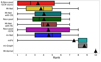
Figure 1: Boxplot of ranks of the algorithms across the 20 text datasets. The medians and means of the ranks are shown by the vertical lines and the black triangles respectively; whiskers extend to the minimum and maximum ranks.

Text Categorization

We evaluate the proposed approach on 20 text datasets (Zhou, Sun, and Li 2009) derived from the 20 Newsgroup corpus (details in supplementary).

Aside from the classical MIL models such as MI-Kernel, mi-Graph and mi-FV, we also consider the mi and MI-net models as baselines, as they are shown to outperform the classical models on these datasets in (Wang et al. 2018).

Figure 2: Predictions of voting probability from Deep Sets, DS-GCN, and B-DS-GCN for the 2016 US presidential election. A county is shown in red (or blue) if the majority votes in favor of republican (or democratic) party. The intensity of the red and blue dots indicates the percentage of the votes obtained by the republican and democratic parties respectively.

For this task, we use a residual architecture with pooling as the base model (details in supplementary). We conduct 10 fold cross-validation 10 times using the data-splits of (Zhou, Sun, and Li 2009). The obtained results are summarized in Table 2. The boxplot of the ranks of the algorithms across the 20 datasets is shown in Figure 1.

From Table 2 and Figure 1, we observe that all neural network based models outperform the classical MIL models on average in this task. In particular, MI-Net and MI-Net with DS algorithms show impressive performance. We also see that using the $k$-NN heuristic to construct $\mathcal{G}_{obs}$ does not work well for this task, as the Res+pool-GCN algorithm shows worse performance on average compared to the base model. The proposed B-Res+pool-GCN algorithm outperforms the base model considerably and achieves the best average and median ranks among all algorithms across the 20 datasets.

Electoral Results Prediction

In this task, our aim is to learn to predict the voting pattern of the US counties in the 2016 presidential election. The dataset is obtained from (Flaxman, Wang, and Smola 2015) (details in supplementary). In this dataset, people (instances) are associated with the socio-economical features from US census data and we construct the bags by randomly sampling 100 people from each county.

We consider an extreme data-scarce setting, where the data from only 2.5% of counties (amounting to approximately one county per state) are used for training. We conduct 100 trials where each trial consists of a random train-test split and random sampling of people to construct the bag feature matrix. $\mathcal{G}_{obs}$ is a $k$-NN graph constructed based on the locations of the centroids of the counties.

We choose Deep Sets (DS) (Zaheer et al. 2017) as a non-graph MIL baseline. Its GCN variant DS-GCN uses $\mathcal{G}_{obs}$ for graph convolution. In order to compute the distance matrix for the non-parametric graph inference step of the proposed Bayesian DS-GCN (B-DS-GCN) algorithm, we use the bag embeddings obtained from the DS-GCN (details in supplementary). We also compare our results with standard MIL baselines, such as MI-Kernel and mi-SVM.

Table 3: Average accuracy and ND (in %) of electoral results prediction reported with std. error over 100 trials.

Algorithm	MI-Kernel	mi-SVM	Deep Sets	DS-GCN	B-DS-GCN
Accuracy	63.45$\pm$6.10	72.17$\pm$9.10	73.22$\pm$3.22	74.05$\pm$4.56*	74.29$\pm$3.15*
ND	N/A	N/A	22.35$\pm$2.66	21.61$\pm$3.17	21.47$\pm$2.45

We conduct a Wilcoxon signed rank test to assess the statistical significance of the obtained results. For the BGCN (or GCN) variant of the base model, * indicates that the performance of the algorithm is significantly better at the 5% level compared to the base model. Similarly, ** for the BGCN (or GCN) variant refers to significantly better performance compared to both the base model and its GCN (or BGCN) variant. This procedure is followed in the next experiment as well.

Table 3 reports the classification accuracy (republican vs. democrat) and the Normalized Deviation (ND) of the predicted percentage of votes in each county. We observe that the DS-GCN outperforms Deep Sets, since the latter cannot incorporate spatial information. The proposed B-DS-GCN algorithm achieves the highest average accuracy and the lowest average ND. Figure 2 shows that compared to Deep Sets and DS-GCN, the predicted voting percentages from the proposed B-DS-GCN algorithm show greater agreement to the ground truth.

Rental Price Prediction

As the last task, we evaluate our model in a distribution regression setting to predict mean rental price in New York City neighborhoods. The dataset includes features of 50,000 rental properties in New York City along with their geographical locations. Each listing (instance) is described by a vector of features such as a text description, the number of bedrooms, bathrooms, etc. (detailed description and visualization in supplementary).

We follow the pre-processing steps described in (Valkanas, Regol, and Coates 2020) that include outlier removal, feature standardization, and removing listings with missing attributes. An observed graph ($\mathcal{G}_{obs}$) of 77 nodes is created using data from the official New York City neighborhood map. Each neighborhood is defined as a node in the graph and we connect nodes with edges based on whether the neighborhoods share a border. The bags are constructed by randomly sampling 25 listings from each neighborhood. For each bag, the label is the true mean of rent prices for all listings within that neighborhood.

We use Root Mean Squared Error (RMSE), Mean Absolute Error (MAE), and Mean Absolute Percentage Error (MAPE) of the predicted average rent as evaluation metrics. We repeat the experiment 100 times using a random 70%-30% train-test split of the bags and random sampling of the listings in those bags in each trial. We consider Deep Sets (DS) (Zaheer et al. 2017) and Set Transformer (ST) (Lee et al. 2019) as the two graph agnostic baselines for this regression task. Their GCN variants DS-GCN and ST-GCN and BGCN variants B-DS-GCN and B-ST-GCN are constructed as in the previous experiment (details in supplementary).

The results are summarized in Table 4. We observe that both DS-GCN and ST-GCN outperform their corresponding base models significantly, which shows that the utilization of spatial information encoded by $\mathcal{G}_{obs}$ is beneficial for the task. The proposed B-DS-GCN and B-ST-GCN provide further improvement in almost all cases. This suggests that beyond simple geographical proximity, the proposed approach is capable of learning more complex relationships among the neighborhoods influencing the mean rental prices.

Table 4: Average RMSE, MAE, and MAPE for rental price prediction reported with std. error over 100 trials.

Algorithm	RMSE	MAE	MAPE (%)
Deep Sets	86.37$\pm$20.41	65.19$\pm$15.72	2.24$\pm$0.36
DS-GCN	78.57$\pm$16.06*	59.21$\pm$10.20*	1.92$\pm$0.24*
B-DS-GCN	67.51$\pm$16.39**	47.24$\pm$10.21**	1.83$\pm$0.20**
Set Transformer	76.34$\pm$15.04	56.09$\pm$9.10	2.02$\pm$0.22
ST-GCN	71.86$\pm$14.65*	53.56$\pm$9.11*	1.81$\pm$0.22*
B-ST-GCN	69.44$\pm$16.23**	49.72$\pm$9.60**	1.83$\pm$0.22*

Table 5: Ablation study for rental price prediction: average RMSE, MAE, and MAPE with std. error over 100 trials.

	Algorithm	RMSE	MAE	MAPE (%)
DS	t. n. d.	75.26$\pm$16.99	54.48$\pm$12.01	2.03$\pm$0.25
	t. n. d. during training	68.15$\pm$16.77*	48.08$\pm$10.77*	1.85$\pm$0.22*
	transductive	67.51$\pm$16.39*	47.24$\pm$10.21*	1.83$\pm$0.20**
ST	t. n. d.	89.95$\pm$23.23	67.12$\pm$18.34	2.29$\pm$0.47
	t. n. d. during training	71.72$\pm$16.50*	51.66$\pm$10.23*	1.88$\pm$0.26*
	transductive	69.44$\pm$16.23**	49.72$\pm$9.60**	1.83$\pm$0.22**

We conduct an ablation study to determine if the transductive setting employed in this work is indeed beneficial. For both architectures, we consider a scenario with ‘test nodes disconnected’ (t. n. d.), which refers to the case where graph inference is carried out for the training nodes only, and disconnected test nodes are added to the graph of training nodes during testing. The other setting is ‘test nodes disconnected during training’, where the training is carried out based on the inferred graph of training nodes, but the learned model is evaluated on the inferred graph of both training and test set nodes. From the results in Table 5, we note that both conducting the non-parametric graph inference for training and test set nodes together and training the model in a transductive setting contribute positively to the outcome of this task.

Conclusion

In this paper, we have proposed a novel graph-based MIL method that is capable of addressing learning problems where there is relational information between the bags to be labeled. We employ a Bayesian graph neural network framework which allows a graph to be inferred from the data, so our method is also applicable to the traditional MIL setting where no graph is specified. The proposed methodology is generally applicable to diverse MIL problem settings, as it can incorporate various existing deep learning based MIL models to learn bag representations and aggregate them using a Bayesian GNN via end-to-end training. Empirical results demonstrate that the proposed method achieves performance comparable to the state-of-the-art on MIL benchmark datasets, and offers better performance in text categorization, electoral results prediction, and rental price regression. Some potential future research directions include adapting the methodology to the inductive setting by using inductive GNN variants (Hamilton, Ying, and Leskovec 2017) and improving the training efficiency of the overall architecture by using node or graph sampling (Chiang et al. 2019; Zeng et al. 2020).

References

- Andrews, Tsochantaridis, and Hofmann (2002) Andrews, S.; Tsochantaridis, I.; and Hofmann, T. 2002. Support vector machines for multiple-instance learning. In Proc. Adv. Neural Info. Process. Syst.
- Chiang et al. (2019) Chiang, W.-L.; Liu, X.; Si, S.; Li, Y.; Bengio, S.; and Hsieh, C.-J. 2019. Cluster-GCN: An efficient algorithm for training deep and large graph convolutional networks. In Proc. ACM SIGKDD Int. Conf. Knowl. Discov. and Data Mining.
- Deselaers and Ferrari (2010) Deselaers, T.; and Ferrari, V. 2010. A conditional random field for multiple-instance learning. In Proc. Int. Conf. Machine Learning.
- Dietterich, Lathrop, and Lozano-Pérez (1997) Dietterich, T. G.; Lathrop, R. H.; and Lozano-Pérez, T. 1997. Solving the multiple instance problem with axis-parallel rectangles. Artificial Intell., 89(1): 31–71.
- Elinas, Bonilla, and Tiao (2020) Elinas, P.; Bonilla, E. V.; and Tiao, L. C. 2020. Variational inference for graph convolutional networks in the absence of graph data and adversarial settings. In Proc. Adv. Neural Info. Process. Syst.
- Flaxman, Wang, and Smola (2015) Flaxman, S. R.; Wang, Y.-X.; and Smola, A. J. 2015. Who supported Obama in 2012? Ecological inference through distribution regression. In Proc. ACM SIGKDD Int. Conf. Knowl. Discov. and Data Mining.
- Gal and Ghahramani (2016) Gal, Y.; and Ghahramani, Z. 2016. Dropout as a Bayesian approximation: Representing model uncertainty in deep learning. In Proc. Int. Conf. Machine Learning.
- Gärtner et al. (2002) Gärtner, T.; Flach, P. A.; Kowalczyk, A.; and Smola, A. J. 2002. Multi-instance kernels. In Proc. Int. Conf. Machine Learning.
- Hamilton, Ying, and Leskovec (2017) Hamilton, W.; Ying, Z.; and Leskovec, J. 2017. Inductive representation learning on large graphs. In Proc. Adv. Neural Info. Process. Syst.
- Ilse, Tomczak, and Welling (2018) Ilse, M.; Tomczak, J.; and Welling, M. 2018. Attention-based deep multiple instance learning. In Proc. Int. Conf. Machine Learning.
- Jiang et al. (2019) Jiang, B.; Zhang, Z.; Tang, J.; and Luo, B. 2019. Graph optimized convolutional networks. arXiv e-prints : arXiv 1904.11883.
- Kalofolias (2016) Kalofolias, V. 2016. How to learn a graph from smooth signals. In Proc. Artificial Intell. and Statist.
- Kalofolias and Perraudin (2019) Kalofolias, V.; and Perraudin, N. 2019. Large scale graph learning from smooth signals. In Proc. Int. Conf. Learning Representations.
- Kipf and Welling (2017) Kipf, T.; and Welling, M. 2017. Semi-supervised classification with graph convolutional networks. In Proc. Int. Conf. Learning Representations.
- Lee et al. (2019) Lee, J.; Lee, Y.; Kim, J.; Kosiorek, A. R.; Choi, S.; and Teh, Y. W. 2019. Set transformer: A framework for attention-based permutation-invariant neural networks. In Proc. Int. Conf. Machine Learning.
- Liu, Wu, and Zhou (2012) Liu, G.; Wu, J.; and Zhou, Z.-H. 2012. Key instance detection in multi-instance learning. In Proc. Asian Conf. Machine Learning.
- Ma et al. (2019) Ma, J.; Tang, W.; Zhu, J.; and Mei, Q. 2019. A flexible generative framework for graph-based semi-supervised learning. In Proc. Adv. Neural Info. Process. Syst.
- Pal et al. (2020) Pal, S.; Malekmohammadi, S.; Regol, F.; Zhang, Y.; Xu, Y.; and Coates, M. 2020. Non-parametric graph learning for Bayesian graph neural networks. In Proc. Conf. Uncertainty Artificial Intell.
- Pathak et al. (2015) Pathak, D.; Shelhamer, E.; Long, J.; and Darrell, T. 2015. Fully convolutional multi-class multiple instance learning. In Workshop Track Proc. Int. Conf. Learning Representations.
- Quellec et al. (2017) Quellec, G.; Cazuguel, G.; Cochener, B.; and Lamard, M. 2017. Multiple-instance learning for medical image and video analysis. IEEE Rev. Biomed. Engineering, 10: 213–234.
- Ramon and De Raedt (2000) Ramon, J.; and De Raedt, L. 2000. Multi instance neural networks. In Proc. Workshop Attribute-Value and Relational Learning, Int. Conf. Machine Learning.
- Raykar et al. (2008) Raykar, V. C.; Krishnapuram, B.; Bi, J.; Dundar, M.; and Rao, R. B. 2008. Bayesian multiple instance learning: Automatic feature selection and inductive transfer. In Proc. Int. Conf. Machine Learning.
- Sun and Lam (2013) Sun, C.; and Lam, K.-M. 2013. Multiple-kernel, multiple-instance similarity features for efficient visual object detection. IEEE Tran. Image Process., 22(8): 3050–3061.
- Tu et al. (2019) Tu, M.; Huang, J.; He, X.; and Zhou, B. 2019. Multiple instance learning with graph neural networks. arXiv preprint: arXiv 1906.04881.
- Valkanas, Regol, and Coates (2020) Valkanas, A.; Regol, F.; and Coates, M. 2020. Learning from networks of distributions. In Proc. Asilomar Conf. Signals, Syst. and Comp.
- Wan et al. (2021) Wan, S.; Pan, S.; Yang, J.; and Gong, C. 2021. Contrastive and generative graph convolutional networks for graph-based semi-supervised learning. In Proc. AAAI Conf. Artificial Intell.
- Wang et al. (2018) Wang, X.; Yan, Y.; Tang, P.; Bai, X.; and Liu, W. 2018. Revisiting multiple instance neural networks. Pattern Recognition, 74: 15–24.
- Wei, Wu, and Zhou (2017) Wei, X.; Wu, J.; and Zhou, Z. 2017. Scalable algorithms for multi-instance learning. IEEE Trans. Neural Networks and Learning Syst., 28(4): 975–987.
- Yin et al. (2019) Yin, S.; Peng, Q.; Li, H.; Zhang, Z.; You, X.; Liu, H.; Fischer, K.; Furth, S. L.; Tasian, G. E.; and Fan, Y. 2019. Multi-instance deep learning with graph convolutional neural networks for diagnosis of kidney diseases using ultrasound imaging. In Proc. Uncertain. Safe Utilization Machine Learning Medical Imaging and Clinical Image-Based Procedures, 146–154.
- Zaheer et al. (2017) Zaheer, M.; Kottur, S.; Ravanbakhsh, S.; Póczos, B.; Salakhutdinov, R.; and Smola, A. J. 2017. Deep sets. In Proc. Adv. Neural Info. Process. Syst.
- Zeng et al. (2020) Zeng, H.; Zhou, H.; Srivastava, A.; Kannan, R.; and Prasanna, V. 2020. GraphSAINT: Graph sampling based inductive learning method. In Proc. Int. Conf. Learning Representations.
- Zhang et al. (2011) Zhang, D.; Liu, Y.; Si, L.; Zhang, J.; and Lawrence, R. D. 2011. Multiple instance learning on structured data. In Proc. Adv. Neural Info. Process. Syst.
- Zhang and Goldman (2001) Zhang, Q.; and Goldman, S. A. 2001. EM-DD: an improved multiple-instance learning technique. In Proc. Adv. Neural Info. Process. Syst.
- Zhang et al. (2019) Zhang, Y.; Pal, S.; Coates, M.; and Üstebay, D. 2019. Bayesian graph convolutional neural networks for semi-supervised classification. In Proc. AAAI Conf. Artificial Intell.
- Zhou, Sun, and Li (2009) Zhou, Z.-H.; Sun, Y.-Y.; and Li, Y.-F. 2009. Multi-instance learning by treating instances as non-i.i.d. samples. In Proc. Int. Conf. Machine Learning.