On Gauge Consistency In Gauge-Fixed Yang-Mills Theory

Abstract

We investigate BRST invariance in Landau gauge Yang-Mills theory with functional methods. To that end, we solve the coupled system of functional renormalisation group equations for the momentum-dependent ghost and gluon propagator, ghost-gluon, and three- and four-gluon vertex dressings. The equations for both, transverse and longitudinal correlation functions are solved self-consistently: all correlation functions are fed back into the loops. Additionally, we also use the Slavnov-Taylor identities for computing the longitudinal correlation functions on the basis of the above results. Then, the gauge consistency of the solutions is checked by comparing the respective longitudinal correlation functions. We find good agreement of these results, hinting at the gauge consistency of our setup.

I Introduction

Infrared QCD is a strongly correlated system that is governed by confinement and spontaneous chiral symmetry breaking, whose understanding and resolution require numerical non-perturbative first principle approaches. Functional diagrammatic approaches such as the functional renormalisation group (fRG) and Dyson-Schwinger equations (DSE), or $n$-particle irreducible approaches (nPI) potentially offer both, analytic access to the mechanisms behind the infrared dynamics of QCD as well as its quantitative numerical resolution. For recent reviews on fRG and DSE approaches to QCD see [1, 2].

The diagrammatic nature of functional approaches is best implemented within gauge-fixed QCD, for a recent discussion of gauge invariant alternatives see [2] and references therein. A specifically well-suited gauge fixing is the Landau gauge, in particular for numerical applications. The latter require truncations to the infinite hierarchy of coupled loop equations for correlation functions in functional approaches. Then, the strongly correlated nature of infrared QCD begs the question of whether the truncations commonly used for explicit numerical solutions transport the underlying gauge symmetry of QCD: are the correlation functions computed gauge consistent. Naturally, the gauge consistency of the correlation functions is essential for confinement, both its manifestation in gauge-fixed approaches as well as its understanding.

In the present work, we put forward a systematic approach towards the evaluation of the above question: First, one computes transverse and longitudinal correlation functions in QCD with functional approaches. Then, the gauge consistency of the results is tested by inserting them into the Slavnov-Taylor identities (STIs). The STIs encode the changes of gauge-fixed correlation functions under gauge or BRST-transformations.

The evaluation of the latter test comes with an intricacy. The STIs also constitute a set of functional relations for correlation functions. These relations can be derived from the BRST identity of the effective action, the BRST master equation, similarly to deriving functional relations from the fRG-flow of the effective action or the functional DSE for the latter. In the case of the STIs, longitudinal correlation functions are related to combinations of transverse and longitudinal correlation functions. In summary, fRG equations, DSEs, and STIs represent different resummation schemes for correlation functions. While their exact solutions agree, any approximations thereof will not coincide in general. To exemplify this situation, let us emphasise that one can easily guarantee the STIs for a finite set of correlation functions in a given order of the truncation if simply using the STIs for the computation of the longitudinal correlation functions. Evidently, this resolution of the STIs does not guarantee the gauge consistency of the transverse correlation functions. This is best seen in the Landau gauge, where the set of functional relations for transverse correlation functions is decoupled from the system of longitudinal ones. Instead, gauge consistency should rather be evaluated by the smallness of the deviations of correlation functions within all functional relations at hand: fRG flows, DSEs, STIs and $n$PI-relations. For a detailed discussion of these subtleties, see [2, 3].

In the present work, we study Landau gauge Yang-Mills theory within a systematic vertex expansion with the functional renormalisation group. Longitudinal correlation functions are also computed from their respective Slavnov-Taylor identities, which follow from the BRST master equation for the effective action. This task is facilitated with the code framework QMeS-Derivation [4, 5], that allows for the derivation of fRG and DSE equations as well as (m)STIs. We use an advanced truncation for these computations, even though fully quantitative computations are still more advanced, see in particular [6, 7]. The respective results are also compared with the corresponding lattice results. In Section III we discuss the consequences for the gauge consistency of the present results as well as extensions of the current computations. Section IV contains a brief conclusion to the present work. The Appendices Appendix A, Appendix B and Appendix C contain some technical details of the computation and the diagrammatic functional equations within the truncation used throughout this work are shown in Appendix D.

II Slavnov-Taylor Identities in Functional Approaches

We consider $SU(N_{c})$ Yang-Mills theory in Euclidean space-time within the Landau gauge. The explicit results are obtained in the physical (QCD) case $N_{c}=3$, but they readily extend to general $N_{c}$. The approximation used here carries the large $N_{c}$ scaling which is present in the dominant tensor structure, for a respective discussion see [8]. The gauge-fixed classical action, including the ghost term and BRST source terms, is given by

$$S= \,\int_{x}\Biggl{[}\frac{1}{4}F^{a}_{\mu\nu}F^{a}_{\mu\nu}+\partial_{\mu}\bar{c}^{a}D^{ab}_{\mu}c^{b}+B^{a}\partial_{\mu}A_{\mu}^{a}-\frac{\xi}{2}B^{a}B^{a}$$

$$-Q_{A,\mu}^{a}D^{ab}_{\mu}c^{b}-\frac{1}{2}gf^{abc}Q_{c}^{a}c^{b}c^{c}+Q_{\bar{c}}^{a}B^{a}\Biggr{]}\,,$$ (1)

where we have introduced the shorthand notation $\int_{x}=\int d^{4}x$. The covariant derivative $D$ in the adjoint representation and the field strength tensor are defined as,

$$D^{ab}_{\mu}c^{b}= \,\partial_{\mu}c^{a}+gf^{acb}A^{c}_{\mu}c^{b}\,,$$

$$F_{\mu\nu}^{a}= \,\partial_{\mu}A_{\nu}^{a}-\partial_{\nu}A_{\mu}^{a}+gf^{abc}A_{\mu}^{b}A_{\nu}^{c}\,,$$ (2)

and the Landau gauge is implemented with $\xi\rightarrow 0$. The action 1 depends on the superfield $\Phi$,

$$\Phi=(A_{\mu},c,\bar{c},B)\,,\qquad Q=(Q_{A},Q_{c},Q_{\bar{c}})\,,$$ (3)

and we have already introduced source terms the BRST transformations (Becchi, Rouet, Stora, Tyutin) [9, 10] of the fields $\delta_{\text{BRST}}\Phi_{a}=\mathfrak{s}\Phi_{a}\delta\lambda$ in a general covariant gauge, coupled to the currents $Q_{\Phi_{a}}$. The respective transformations are given by

$$\mathfrak{s}A_{\mu}^{a} =D^{ab}_{\mu}c^{b}\,,$$

$$\mathfrak{s}c^{a} =\frac{1}{2}gf^{abc}c^{b}c^{c}\,,$$

$$\mathfrak{s}\bar{c}^{a} =B^{a}\,,$$

$$\mathfrak{s}B^{a} =0\,,$$ (4)

with the Nakanishi-Lautrup field $B^{a}$. Evidently, we do not need $Q_{B}$, as the respective BRST transformation vanishes identically. Moreover, with $\mathfrak{s}^{2}=0$ these additional terms are also BRST invariant. Our general conventions and notation follows [4].

II.1 Functional Renormalisation Group

In the functional renormalisation group approach, an infrared cutoff is introduced by adding momentum-dependent mass terms $\Delta S_{k}$ to the classical action $S[\Phi,Q]$ defined in 1,

$$\Delta S_{k}=\int\left(\frac{1}{2}(R_{A})^{ab}_{\mu\nu}\,A^{a}_{\mu}A^{b}_{\nu}+(R_{c})^{ab}\,\bar{c}^{a}c^{b}\right)\,,$$ (5)

with the infrared cutoff scale $k$. The regulators $R=(R_{A},R_{c})$ suppress quantum fluctuations for momenta $p^{2}\lesssim k^{2}$ for the respective fields, and vanish for $p^{2}\gtrsim k^{2}$. The specific form of the regulators used in the present work can be found in Section B.3. The infrared regularised classical action $S+\Delta S_{k}$ is then used in the path integral representation of the generating functional $Z[J,Q]$. Here, the super-current $J$ includes currents for all component fields $J=(J_{A},J_{c},J_{\bar{c}},J_{B})$.

The functional flow equation is derived for the scale-dependent effective action

$$\Gamma_{k}[\Phi,Q]=\int J\cdot\Phi-\log Z[J,Q]-\Delta S_{k}[\Phi]\,,$$ (6)

the modified Legendre transform of the Schwinger functional $\log Z$. Its logarithmic scale derivative provides us with the one-loop exact fRG equation,

$$\partial_{t}\Gamma_{k}=\int_{x}\left[\frac{1}{2}(\dot{R}_{A})^{ab}_{\mu\nu}\,(G_{AA})_{\mu\nu}^{ab}-(\dot{R}_{c})^{ab}(G_{c\bar{c}})^{ab}\right](x,x)\,,$$ (7)

with $\dot{R}=\partial_{t}R$, the (negative) RG time $t=\ln(k/\Lambda)$, and the full ghost and gluon propagators

$$G_{AA}=\left[\frac{1}{\Gamma^{(2)}+R}\right]_{AA}\,,\qquad G_{c\bar{c}}=\left[\frac{1}{\Gamma^{(2)}+R}\right]_{c\bar{c}}\,.$$ (8)

Here, $\Lambda$ is a reference scale, typically chosen to be the initial cutoff scale deep in the ultraviolet (UV). If the initial scale is chosen sufficiently large, the effective action tends towards the local UV effective action $\Gamma_{\Lambda}$ that consists out of all UV-relevant terms. For Yang-Mills theory this UV effective action includes all terms in the classical action as well as a mass term for the gluon. The latter term originates in the breaking of gauge invariance via the regulator term for $k\neq 0$. In turn, for $k\to 0$, this breaking disappears and we are left with the full BRST invariant effective action. For a full derivation and further discussions, see e.g. [4, 11] and the QCD-related reviews [12, 13, 14, 15, 16, 17, 2].

At this point we would like to remark on some implicit assumptions within the derivation of the flow equation 7: it implies that the only $k$-dependence of the renormalised generating functional originates in the cutoff term. Then, in particular, the renormalisation procedure is assumed to be $k$-independent, for a detailed discussion see e.g. [14, 16]. While the self-consistency of this assumptions is readily shown for the wave function renormalisations and vertices, the absence of a mass renormalisation for the gluon is less trivial and potentially affects the underlying BRST invariance. This question is of utmost importance for the interpretation of Yang-Mills theory in the presence of the infrared cutoff term as a deformation of Yang-Mills theory, rather than a massive extension of Yang-Mills theory, for the Curci-Ferrari (CF) model see e.g. [18, 19, 20, 21, 22]. In the CF model, masses for ghost and gluons are part of the gauge fixing. In contrast, one may also simply add a gluonic mass term after the gauge fixing, and the two procedures agree in the Landau gauge. Note also, that the latter procedure is similar to adding the regulator term to the gauge-fixed action in the fRG approach, a subtle difference being the mass renormalisation and the related classical BRST symmetry.

Both procedures have to be contrasted to massive extensions of Yang-Mills theory, where the mass is added to the classical action without a gauge fixing, bound to introduce non-localities.

We close with the remark that the massless limit of massive extensions of Yang-Mills theory is an intricate one as it defines a flow in theory space. Instead, the removal of the momentum-local infrared regulator in Yang-Mills theory is smooth, as the cutoff term can be interpreted as the local deformation of Yang-Mills theory. Still, even for local deformations the correct description of the massless limit is intricate as we shall see later, see in particular Section II.4.

II.2 STI & mSTI

Classical BRST symmetry with the infinitesimal transformations 4 leads to symmetry identities on the quantum level, that can be formulated in terms of a master equation, see e.g. [23, 24],

$$\int_{x}\left(\frac{\delta\Gamma}{\delta Q_{A,\mu}^{a}}\frac{\delta\Gamma}{\delta A_{\mu}^{a}}+\frac{\delta\Gamma}{\delta Q_{c}^{a}}\frac{\delta\Gamma}{\delta c^{a}}+\frac{\delta\Gamma}{\delta Q_{\bar{c}}^{a}}\frac{\delta\Gamma}{\delta\bar{c}^{a}}\right)=0\,,$$ (9)

and integrating out the (Gaußian) Nakanishi-Lautrup field $B$ converts Equation 9 into

$$\int_{x}\left(\frac{\delta\Gamma}{\delta Q_{A,\mu}^{a}}\frac{\delta\Gamma}{\delta A_{\mu}^{a}}+\frac{\delta\Gamma}{\delta Q_{c}^{a}}\frac{\delta\Gamma}{\delta c^{a}}-\frac{1}{\xi}(\partial_{\nu}A^{a}_{\nu})\partial_{\mu}\frac{\delta\Gamma}{\delta Q_{A,\mu}^{a}}\right)=0\,.$$ (10)

In the derivation of 10 one also uses the fact that the anti-ghost field only appears linearly in the action.

Finally, the introduction of the cutoff term 5 leads to a modification of the symmetry identities 9 or 10, the modified Slavnov-Taylor identity (mSTI). It is derived similarly to the flow equation 7: there the right hand side can be interpreted as the equation which governs the violation of scale invariance. For the mSTI, the additional term in comparison to 9 or 10 originates from the lack of BRST invariance of the regulator term. As for the flow equation, it is a one-loop exact equation. In the presence of the Nakanishi-Lautrup field $B$, the mSTI takes the concise form,

$$\int_{x}\Gamma_{Q_{i}}\Gamma_{\Phi_{i}}=\int_{x,y}\,\left(R\,G\right)_{\Phi_{i}\Phi_{j}}\,\Gamma_{Q_{j}\Phi_{i}}$$ (11)

with the notation

$$\Gamma_{Q_{1}\cdots Q_{n}\Phi_{n+1}\cdots\Phi_{n+m}}=\frac{\delta\Gamma[\Phi,Q]}{\delta{Q_{1}}\cdots\delta{Q_{n}}\delta\Phi_{n+1}\cdots\delta{\Phi_{n+m}}}\,,$$ (12)

for mixed derivatives of the effective action with respect to BRST currents and fields. The integral $\int_{x,y}$ on the right-hand side of 11 constitutes a space-time trace of the product of operators $(R\,G)(x,y)$ and $\Gamma_{Q\Phi}(y,x)$. On both sides of 11, a sum over species of fields as well as internal and Lorentz indices is implied. For example, the left-hand side of 11 is simply that of 9, if re-instating all indices.

As already mentioned above, the right-hand side of 11 originates in the breaking of BRST invariance induced by the regulator term, similarly to the right-hand side of the flow equation, which manifests the breaking of scale invariance induced by the regulator term. We emphasise, that 11 is derived with the same implicit assumption of the independence of the UV renormalisation procedure of the cutoff term. We will discuss the self-consistency of this assumption in Section II.4.

For $k\rightarrow 0$ the mSTI reduces to the STI. Thus, satisfying the mSTI at all scales $k$, guarantees gauge invariance of observables at $k=0$. Modified Slavov-Taylor identities, Ward identities and Nielsen identities have been studied intensively in the fRG approach as they are key to quantitatively reliable approximations in gauge theories. For a partial use for momentum-dependent correlation functions in QCD see [6, 25], for a full derivation and further discussions in the present context, see e.g. [4, 11]. For generic fRG literature on modified symmetry identities see e.g. [26, 27, 28, 29, 30, 31, 32, 33, 34, 14, 35, 36, 37, 38, 39, 6, 40, 41, 25, 42, 43, 44, 45, 46], a complete list of references can be found in the recent review see [2].

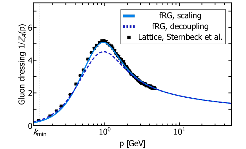
(a) Gluon dressing $1/Z_{A}(p)$.

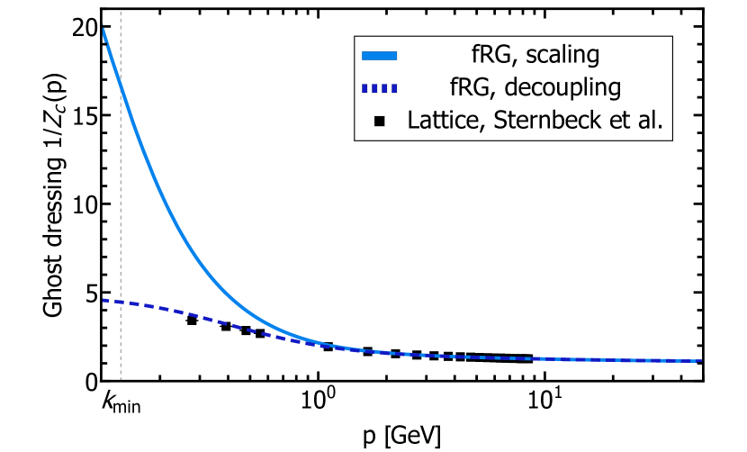
(b) Ghost dressing $1/Z_{c}(p)$.

Figure 1: Propagator dressings form the fRG for scaling (solid) and decoupling (dashed) solutions as a function of momentum $p$ in comparison to the lattice results (squares) of [47]. The global normalisation of the lattice results was fixed by our scaling solution, c.f. Section B.4.

II.3 Vertex Expansion and Truncations

We expand the effective action in terms of $\Phi$ and $Q$ vertices. At vanishing BRST current, $Q=0$, this entails,

$$\Gamma_{k}[\Phi,0]=\sum_{n=1}^{\infty}\int\frac{1}{n!}\Gamma_{\Phi_{1}\cdots\Phi_{n}}\Phi_{n}\dots\Phi_{1}\,,$$ (13)

with the superfield $\Phi$ introduced 3, the 1PI correlation functions $\Gamma_{\Phi_{1}\cdots\Phi_{n}}$, and the normalisation $\Gamma_{k}[0,0]=0$. The prefactor $1/n!$ is a vector-factorial, where each component corresponds to the factorial of the number of fields of the same species in the summand. Including BRST and mixed vertices is done analogously. Inserting the vertex expansion 13 into the fRG equation 7, one sees readily, that a full solution of the theory requires the complete set of 1PI correlation functions. Specifically, the flow of an $n$-point correlation function $\Gamma_{\Phi_{1}\cdots\Phi_{n}}$ depends on correlation functions $\Gamma_{\Phi_{1}\cdots\Phi_{m}}$ with $2\leq m\leq n+2$. This leads to an infinite tower of coupled integral-differential equations. For most practical purposes this tower has to be truncated. Similar considerations apply to all closed functional master equations and in particular to the set of DSEs, whose towers of coupled integral equations also satisfy $2\leq m\leq n+2$. For a complete survey on results for Landau gauge correlation functions we refer to the reviews [2, 48, 49, 50, 51, 52, 53, 22].

For this work, we restrict ourselves to the truncation shown in Figure 18 in the appendix. The gluon and ghost propagators are obtained from their respective two-point functions via 8. The two-point functions read

$$\Gamma_{AA,\mu\nu}^{ab}(p)= \,\Pi^{\perp}_{\mu\nu}(p)Z_{A}(p)p^{2}\delta^{ab}+\Pi^{\parallel}_{\mu\nu}(p)\Gamma_{AA}^{\parallel}(p)\delta^{ab}\,,$$

$$\Gamma_{\bar{c}c}^{ab}(p)= \,Z_{c}(p)p^{2}\delta^{ab}\,,$$ (14)

with the transverse and longitudinal projection operators,

$$\Pi^{\perp}_{\mu\nu}(p)=\,\left(\delta_{\mu\nu}-\frac{p_{\mu}p_{\nu}}{p^{2}}\right)\,,\qquad\Pi^{\parallel}_{\mu\nu}(p)=\,\frac{p_{\mu}p_{\nu}}{p^{2}}\,.$$ (15)

The ghost and gluon dressing functions obtained from our computation are depicted in Figure 1. The respective gluon propagator is shown in Figure 2. There, the present results are compared to lattice data. For recent results see in particular [6] (fRG) and [7, 54, 55, 56, 57] (DSE).

The longitudinal scalar part $\Gamma_{AA}^{\parallel}$ in 14 contains the gauge fixing part that diverges in the Landau gauge limit $\xi\to 0$ and a regular contribution, that originates from the breaking of BRST invariance for finite $k$ and vanishes in the limit $k\to 0$. For $k\neq 0$ we have

$$\Gamma_{AA}^{\parallel}(p)=\frac{1}{\xi}p^{2}+\Gamma_{AA,\textrm{reg}}^{\parallel}\,.$$ (16)

We remark that in the Landau gauge limit the gluon propagator is transverse and does not depend on $\Gamma_{AA,\textrm{reg}}^{\parallel}$, even though the latter contribution does not vanish. This is one of the properties that singles out the Landau gauge not only as the technically least difficult Lorenz gauge, but also suggests the best convergence of the results for correlation functions in a systematic vertex expansions: for any other choice of $\xi$ the regular part $\Gamma_{AA,\textrm{reg}}^{\parallel}$ feeds back into the dynamics of the system, even though its integrated impact has to vanish at vanishing cutoff scale. A more detailed discussion including the consistency of different functional relations (fRG, DSE, mSTI) is deferred to Section II.4.

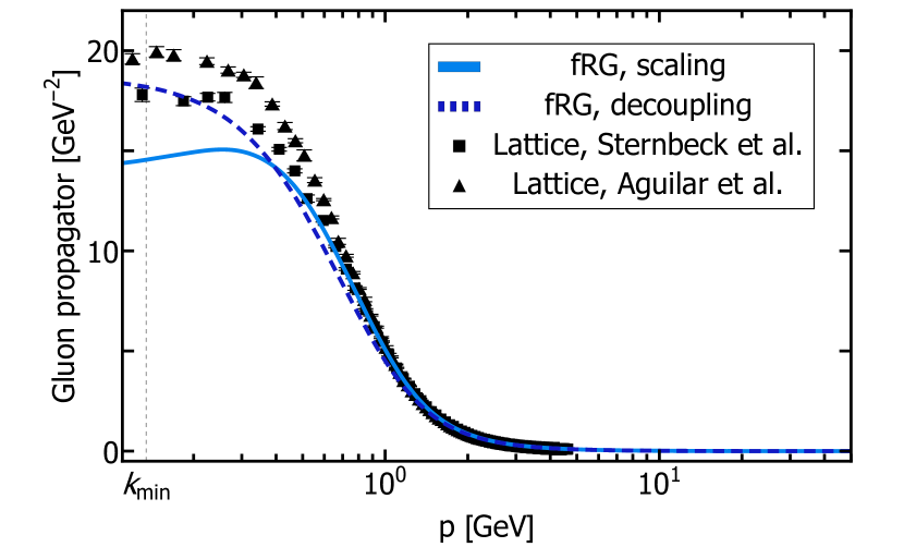
Figure 2: Scaling (solid) and decoupling (dashed) gluon propagator as a function of momentum $p$ in comparison to the lattice data (squares) from [47] and (triangles) from [58]. The global normalisation of the lattice data was fixed by our scaling solution, c.f. Section B.4.

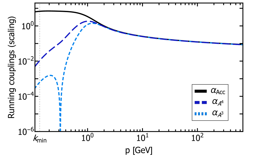
Figure 3: Running couplings as defined in 28 obtained from different Yang-Mills vertex dressings as a function of momentum $p$.

Utilising the projection operators 15, we can split correlation functions into their transverse and longitudinal parts,

$$\Gamma_{\Phi_{1}\cdots\Phi_{n}}= \,\Gamma_{\Phi_{1}\cdots\Phi_{n}}^{\perp}+\Gamma_{\Phi_{1}\cdots\Phi_{n}}^{\parallel}\,,$$ (17)

where $\Gamma_{\Phi_{1}\cdots\Phi_{n}}^{\perp}$ is the completely transverse part of the correlation function, structurally given by $\Gamma_{\Phi_{1}\cdots\Phi_{n}}^{\perp}=(\Pi^{\perp})^{n}\Gamma_{\Phi_{1}\cdots\Phi_{n}}$. The longitudinal part simply is the complement, and hence is built up from correlation functions with at least one longitudinal leg.

We will explain this splitting at the example of the ghost-gluon vertex. Its complete basis is spanned by only two tensor structures: the classical one, proportional to the anti-ghost momentum, and a longitudinal non-classical one, which is proportional to the gluon momentum,

$$\Gamma_{A\bar{c}c,\mu}^{abc}(p,q) =if^{abc}\Bigl{(}\lambda_{A\bar{c}c,\text{cl}}(p,q)q_{\mu}+\lambda_{A\bar{c}c,\text{ncl}}(p,q)p_{\mu}\Bigr{)}\,.$$ (18)

However, we can rewrite this in terms of the projection operator defined in 15, which is transverse in the gluon momentum $p$,

$$\Gamma_{A\bar{c}c,\mu}^{abc}(p,q)= \,if^{abc}\Bigl{(}\lambda_{A\bar{c}c}(p,q)\,\Pi^{\perp}_{\mu\nu}(p)q_{\nu}$$

$$\hskip 56.9055pt+\bar{\lambda}_{A\bar{c}c,1}(p,q)\,p_{\mu}\Bigr{)}\,,$$ (19)

with

$$\lambda_{A\bar{c}c}(p,q) =\lambda_{A\bar{c}c,\text{cl}}(p,q)\,,$$

$$\bar{\lambda}_{A\bar{c}c,1}(p,q) =\frac{p\cdot q}{p^{2}}\lambda_{A\bar{c}c,\text{cl}}(p,q)+\lambda_{A\bar{c}c,\text{ncl}}(p,q)\,.$$ (20)

The singularity of such a split with projection operators at $p=0$ is reflected in the prefactor $p\cdot q/p^{2}$ of the classical dressing in $\bar{\lambda}_{A\bar{c}c,1}(p,q)$. It is matched by the respective one in the transverse projection operator multiplying $\lambda_{A\bar{c}c}(p,q)$. Therefore, for non-singular dressings in 18 we only have a parameterisation singularity.

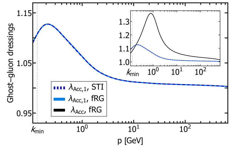
(a) Ghost-gluon vertex dressings.

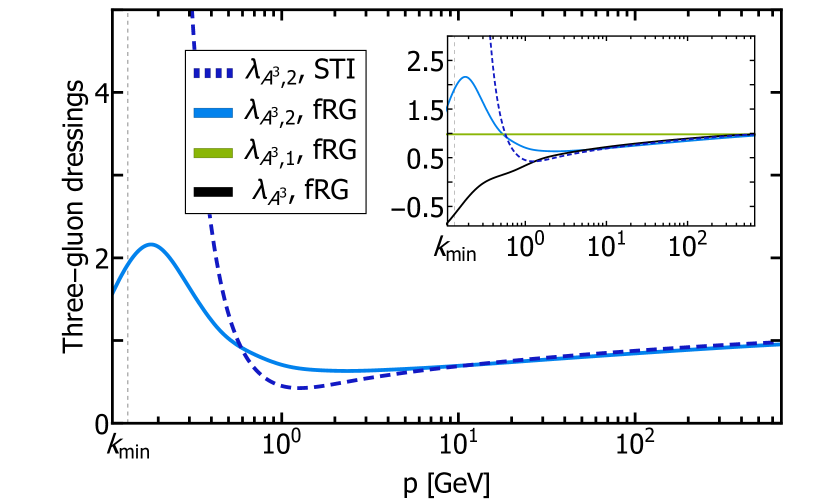
(b) Three-gluon vertex dressings.

Figure 4: Dressings of the three-point functions as a function of momentum $p$. Results from the fRG are shown as solid lines, while STI results are shown as dashed lines. The transverse component is black and the longitudinal ones are depicted in green and blue. Please note that the transverse components are only visible in the insets.

In the present work, we consider relations between the dressings at the symmetric point $p^{2}=q^{2}=-2p\cdot q$. In the ultraviolet limit, the non-classical dressing vanishes and we are left with the classical one. Hence, for the present purpose it is convenient to simply use the longitudinal projection of the classical tensor structure, $\Pi_{\mu\nu}^{\parallel}(p)q_{\nu}$, for the longitudinal part. This leads us to,

$$\Gamma_{A\bar{c}c,\mu}^{abc}(p,q)= \Bigl{(}\lambda_{A\bar{c}c}(p,q)\,\Pi^{\perp}_{\mu\nu}(p)$$

$$\hskip 14.22636pt+\lambda_{A\bar{c}c,1}(p,q)\,\Pi^{\parallel}_{\mu\nu}(p)\Bigr{)}\,\,if^{abc}q_{\nu}\,,$$ (21)

see also [6]. The number index in $\lambda_{A\bar{c}c,1}$ indicates the number of longitudinally projected gluons of the classical tensor structure of the vertex, and no index corresponds to the dressing of the fully transverse tensor structure. The dressing $\lambda_{A\bar{c}c,1}$ is given by

$$\lambda_{A\bar{c}c,1}(p,q)=\lambda_{A\bar{c}c,\text{cl}}(p,q)+\frac{p^{2}}{p\cdot q}\lambda_{A\bar{c}c,\text{ncl}}(p,q)\,.$$ (22)

We have in particular $\bar{\lambda}_{A\bar{c}c,1}(p,q)=-2\lambda_{A\bar{c}c,1}(p,q)$ at the symmetric point. Moreover, for all momenta except those with $p\cdot q=0$, the dressing in 22 has the ultraviolet limit $\lambda_{A\bar{c}c,1}\to\lambda_{A\bar{c}c,\textrm{cl}}$ which facilitates the following discussions. In contradistinction, we find $\bar{\lambda}_{A\bar{c}c,1}\to(p\cdot q)/p^{2}\lambda_{A\bar{c}c,\textrm{cl}}$. In conclusion, the transverse ghost-gluon dressing is equivalent to the classical one, whereas the longitudinal dressing is a combination of the classical and non-classical dressing. For a comparison of the ghost-gluon dressings in 21, see Figure 4(a) and Figure 13 in the Appendix B. For recent results see in particular [6] (fRG) and [7, 58, 59] (DSE).

We now proceed by parametrising the BRST and gluonic vertices in terms of transverse and longitudinal projections analogously to the parameterisation of the ghost-gluon vertex discussed above. With the anti-ghost shift symmetry of the effective action, we can relate the BRST vertices $\Gamma_{cQ_{A}}$ and $\Gamma_{AcQ_{A}}$ to the ghost two-point and the ghost-gluon vertex. A derivation thereof can be found in Section B.6 and we arrive at

$$\Gamma^{ab}_{c\,Q_{A},\mu}(p)= -iZ_{c}(p)p_{\mu}\delta^{ab}\,,$$

$$\Gamma^{abc}_{Ac\,Q_{A},\mu\nu}(p,q)= \,-f^{abc}\Bigr{(}\Pi^{\perp}_{\mu\nu}(p)\lambda_{A\bar{c}c}(p,-q-p)$$

$$\hskip 14.22636pt+\Pi^{\parallel}_{\mu\nu}(p)\lambda_{A\bar{c}c,1}(p,-q-p)\Bigl{)}\,.$$ (23)

Notably, these identities even hold diagramatically true for the flows of the dressings. The other BRST two-point function and vertex are parameterised as,

$$\Gamma^{ab}_{AQ_{\bar{c},}\mu}(p) =-ip_{\mu}\frac{1}{\xi}\delta^{ab}\,,$$

$$\Gamma_{cc\,Q_{c}}^{abc}(p,q) =-if^{abc}\lambda_{Q_{c}cc}(p,q)\,.$$ (24)

In the present work we approximate the three- and four-gluon vertices with their fully dressed classical tensor structures, noted as $\tau_{A^{3},\text{cl}}$ and $\tau_{A^{4},\text{cl}}$. The purely transverse parts are obtained by contracting the classical tensor structure with three and four transverse projection operators respectively. The complements now contain mixed vertices with longitudinal and transverse legs as well as a purely longitudinal part. The parts with at least three longitudinal legs do not contribute since they do not feed back into the diagrams and are therefore not included in our truncation. Thus we parameterise the gluonic vertices as,

$$\Gamma_{A^{3}}(p,q)= \left(\lambda_{A^{3}}\left(\Pi^{\perp}\right)^{3}+\lambda_{A^{3},1}\left(\Pi^{\perp}\right)^{2}\Pi^{\parallel}\right.$$

$$\left.+\lambda_{A^{3},2}\Pi^{\perp}\left(\Pi^{\parallel}\right)^{2}\right)\tau_{A^{3},\text{cl}}+\cdots\,$$

$$\Gamma_{A^{4}}(p,q,r)= \left(\lambda_{A^{4}}\left(\Pi^{\perp}\right)^{4}+\lambda_{A^{4},1}\left(\Pi^{\perp}\right)^{3}\Pi^{\parallel}\right.$$

$$\left.+\lambda_{A^{4},2}\left(\Pi^{\perp}\right)^{2}\left(\Pi^{\parallel}\right)^{2}\right)\tau_{A^{4},\text{cl}}+\cdots\,$$ (25)

where indices and momenta are dropped and the permutations are implicit for the sake of simplicity. The dots indicate terms proportional to $(\Pi^{\parallel})^{n}\tau_{A^{3},\text{cl}}$ and $(\Pi^{\parallel})^{n}\tau_{A^{4},\text{cl}}$ with $n\geq 3$, i.e. with at least $3$ longitudinally projected gluon legs, as well as further, non-classical, tensor structures. We emphasise that for $p\cdot q=0$ or $p\cdot r=0$ the parameterisation in II.3 may lead to parameterisation singularities for the dressings, that are then seen in the respective projections of the diagrams in the functional relations. For further details on the parameterisation, see Section B.1 and e.g. [59] for a similar parametrisation. The longitudinal four-gluon vertices are approximated by their STI-values, see 49. For a comparison of the dressings in II.3 see Figure 4(b) and Figure 5. For recent results see in particular [6] (fRG) and [60, 7, 54, 59] (DSE).

The remaining dressings are obtained from their respective fRG equations, that are depicted in Appendix D in Figure 18. They are evaluated at a symmetric point for three(four)-point functions,

$$p_{i}\cdot p_{j}=\begin{cases}\;\;\;\;p^{2}&\text{for $i=j$,}\\[10.0pt] -\frac{1}{n-1}p^{2}&\text{otherwise, where $n=3(4)$.}\end{cases}$$ (26)

For simplicity, the vertex dressings feeding back into the fRG equations are evaluated at the average momentum configuration $\lambda_{i}(\bar{p})$ with,

$$\bar{p}^{2}=\frac{1}{n}\sum_{i=1}^{n}p_{i}^{2}\,,$$ (27)

which has been shown to be a good approximation, see e.g. [61]. From the transverse dressings we can derive momentum dependent running couplings,

$$\alpha_{A\bar{c}c}(p) =\frac{1}{4\pi}\frac{\lambda_{A\bar{c}c}(p)^{2}}{Z_{A}(p)Z_{c}(p)^{2}}\,,$$

$$\alpha_{A^{3}}(p) =\frac{1}{4\pi}\frac{\lambda_{A^{3}}(p)^{2}}{Z_{A}(p)^{3}}\,,$$

$$\alpha_{A^{4}}(p) =\frac{1}{4\pi}\frac{\lambda_{A^{4}}(p)}{Z_{A}(p)^{2}}\,.$$ (28)

These vertex couplings are perturbatively two-loop degenerate (two-loop universality), leading to

$$\alpha_{A\bar{c}c}(p)\approx\alpha_{A^{3}}(p)\approx\alpha_{A^{4}}(p)\,,\quad\text{for}\quad p\gtrsim 5\,\text{GeV}.$$ (29)

This property is reflected well in our truncation, see Figure 3. We emphasise that 29 is non-trivial, as our initial condition only feature constant vertices. These initial conditions are chosen or tuned such that 29 is fulfilled. Satisfying 29 over several orders of magnitude is already a significant indication for gauge consistency. For a detailed discussion of this aspect see [6] and more information on the tuning procedure is given in Section III.1.

II.4 Functional Relations and Consistency Constraints

The computation of functional relations is facilitated in Landau gauge Yang-Mills theory, if contrasted with general covariant gauges: in the Landau gauge the set of all transverse functional relations is closed, i.e.

$$\Gamma_{(n)}^{\perp}=\text{funRel}^{\perp}_{(n)}[\{\Gamma_{(2\leq m\leq n+2)}^{\perp}\}]\,,$$ (30a)

where $$\{\Gamma_{(2\leq m\leq n+2)}^{\perp}\} m 2\leq m\leq n+2$$ indicates the set of all transverse -point correlation functions with . In contradistinction, the longitudinal correlation functions satisfy

$$\Gamma_{(n)}^{\parallel}=\text{funRel}^{\parallel}_{(n)}[\{\Gamma_{(2<m\leq n+2)}^{\parallel}\},\{\Gamma_{(2\leq m\leq n+1)}^{\perp}\}]\,.$$ (30b)

Note that the longitudinal two-point function $\Gamma_{(2)}^{\parallel}$ does not feed back into the longitudinal relations 30b and 31. Equation 30a follows from the fact that the gluon propagator $G_{A}$ as well as $(G\,\dot{R}\,G)_{AA}$ are transverse in the Landau gauge and so are all internal legs. Also, the propagator only depends on $\Gamma_{(2)}^{\perp}$. The structure 30 applies to fRG equations and DSEs, for more details see [3, 6, 2, 11].

The mSTIs in 11 involve longitudinal and transverse correlation functions. They are similar to 30b, reading

$$\Gamma_{(n)}^{\parallel}=\text{mSTI}_{(n)}[\{\Gamma_{(2<m\leq n+2)}^{\parallel}\},\{\Gamma_{(2\leq m\leq n+1)}^{\perp}\}]\,.$$ (31)

Note that 31 constitutes yet another tower of functional relations for longitudinal correlation functions. Naturally, as for truncated towers of fRG equations and DSEs, its solution for a given truncation will in general differ from both, the solution of the longitudinal fRG equations and the longitudinal DSEs (or any other tower of longitudinal functional relations). Moreover, for a finite set of longitudinal and transverse correlation functions, one may simply use the (m)STI for computing the longitudinal correlation functions. Such a scheme seemingly builds in gauge consistency by construction. Naturally, the longitudinal correlation functions will then in general not satisfy the respective fRG equations or DSEs. In conclusion, it is not the violation of the mSTI alone, which comprises the information about gauge consistency, but the combination of all functional relations.

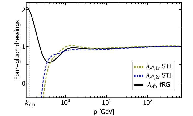
Figure 5: Dressings of the four-point function as a function of momentum $p$. The result from the fRG is shown as a solid line, while STI results are shown as dashed lines. The transverse component is black and the longitudinal ones are depicted in green and blue.

However, even though 31 is very similar to the fRG equations and DSEs for the longitudinal dressings, there is an important structural difference which is most apparent in the Landau gauge limit: while 30a and 30b only depend on the transverse part of the regulator, the mSTI 31 depends on the longitudinal part for regulators whose longitudinal part diverges with $1/\xi$. A natural class of regulators with this property is that of RG-adapted or spectrally adapted regulators, see [14, 62]. In this case, the regulators are proportional to the full dispersion of the respective field, which is detailed in Section B.3. This choice ensures, that the effective action in the presence of the regulator has the underlying RG-invariance of the full theory at vanishing regulator, hence the name RG-adapted. Specifically, the longitudinal part of the gluon regulator reads

$$(R_{A})^{\parallel,ab}_{\mu\nu}(p)= \,\delta^{ab}\Pi^{\parallel}_{\mu\nu}(p)\Gamma^{\parallel}_{AA}(p)\,r\left(\frac{p^{2}}{k^{2}}\right)\,.$$ (32)

The class of regulators with 32 leads to

$$\lim_{\xi\to 0}p_{\mu}(G_{AA}R_{A})_{\mu\nu}=p_{\nu}\frac{r_{A}}{1+r_{A}}(p^{2}/k^{2})\,,$$ (33)

and hence one of the internal lines in the mSTI diagrams has a longitudinal part. In turn, for gluon regulators with a regular longitudinal part we have

$$p_{\mu}(G_{AA}R_{A})_{\mu\nu}\propto\xi p_{\nu}\,,$$ (34)

and hence all internal lines are transverse in the Landau gauge. Then, the mSTI has the same structure as 30b in terms of contributing correlation functions.

Interestingly, the fRG equations and DSEs (in the presence of a regulator), 30, are the same in the Landau gauge limit for regulators with either 33 or 34. However, it can be shown, that the contributions of the longitudinal part of the propagator 33 do not cancel in the mSTI. In particular, the effective gluon mass $m_{k}^{2}$ from the STI only receives contributions from the longitudinal part of $(R_{k}G)_{AA}$. In conclusion, only for gluon regulators whose longitudinal part contains the gauge fixing term $1/\xi p^{2}r(p^{2}/k^{2})$, the effective mSTI gluon mass and that from the fRG flow equation or DSE agree, and the implicit assumption of $k$-independence of the renormalisation procedure is self-consistent. In short, only for RG-adapted regulators we do not implicitly introduce a gluon mass (counter) term on the level of the classical action.

This intricacy emphasises the importance of gauge consistency of the regularisation procedure. The comparison of functional mSTI and fRG/DSE always allows us to choose a longitudinal regulator $R_{A}^{\parallel}$ such that all functional relations are compatible. However, this also implies that gauge consistency of truncated fRG flows or DSEs should rather be checked with a set of correlation functions and not a single one.

Throughout this work we will use RG-adapted regulators 32, which are also gauge consistent, as discussed above. A more detailed study of this intricacy and the general regulator (shape) dependence is still under investigation and will be published elsewhere.

We conclude this section with two remarks. Firstly, for regular correlation functions, one can use the STIs for also extracting a part of the respective transverse correlation functions. Loosely speaking, regularity implies

$$|\partial_{p_{i}}\Gamma_{(n)}|<\infty\,,$$ (35)

in which case the longitudinal and transverse parts are linked. However, in the present case of Yang-Mills theories, it can be shown that regular correlation functions are at odds with confinement. In turn, in perturbation theory, one can show that the regularity assumption holds true. Indeed, it is also related to the identification of running couplings 28. This adds yet another layer of complexity to the current situation: for perturbative and semi-perturbative momenta regularity holds true and we should see the respective relations between longitudinal and transverse correlation functions.

In summary, this leaves us with the necessity as well as a large variety of non-trivial consistency checks. We also emphasise that great care is needed in the interpretation of violations of the mSTI or alternatively of other functional relations for longitudinal correlation functions within truncations.

II.5 Confinement

Confinement describes the effect that no coloured particles can be detected directly by experiments, i.e. the absence of coloured states from the physical asymptotic spectrum of our theory, and is in one-to-one correspondence to a dynamical mass gap $m_{\textrm{gap}}^{\textrm{\tiny YM}}$ in the physical spectrum of Yang-Mills theory. It is fundamentally linked to the non-Abelian gauge group of QCD, and hence it is most cleanly studied in Yang-Mills theory in the absence of dynamical quarks that complicate the matter.

In Landau gauge Yang-Mills theory confinement is in one-to-one correspondence to a mass gap (finite correlation length $\xi_{\textrm{conf}}$) in the gluon propagator, as has been shown in [63, 64]. There, it has been also shown that the confinement-deconfinement temperature $T_{\textrm{conf}}$ is proportional to the (inverse) screening length, $T_{\textrm{conf}}\propto 1/\xi_{\textrm{conf}}$. Moreover, it also sets the scale of the glueball spectrum, $m_{\textrm{glueball}}\propto 1/\xi_{\textrm{conf}}$, and in conclusion $m^{\textrm{\tiny YM}}_{\textrm{gap}}\propto 1/\xi_{\textrm{conf}}$. Finally, it also sets the saturation scale of the effective charge, see [65].

Figure 6: Effective gluon mass $m_{\perp}^{2}$, defined in 36, at $k=k_{\mathrm{min}}$ from different fRG solutions as a function of the difference $m_{\bot,\Lambda}^{2}-m_{\mathrm{ref}}^{2}$ of the mass parameters at the initial cutoff scale $\Lambda$. More details on the effective gluon mass at a finite cutoff scale are deferred to Section B.3. The reference mass $m_{\mathrm{ref}}^{2}$ indicates the initial mass of the extrapolated UV value for the mass parameter of the true scaling solution, see also Section B.3; and the light blue triangle indicates our approximate scaling solution. The black markers correspond to Higgs-type and the blue markers to confining solutions. The dark blue square is used as a representative decoupling solution. The black pentagon is used as a representative Higgs-type solution.

In conclusion, while the mass gap $1/\xi_{\textrm{conf}}$ in the Landau gauge gluon propagator is a property of a gauge-fixed correlation function, it is directly linked to the dynamical mass gap $m_{\textrm{gap}}^{\textrm{\tiny YM}}$ in Yang-Mills theory. At small momenta, the mass gap manifests itself as an effective gluon mass parameter $m_{\perp}^{2}$ in the gluon propagator or transverse gluon two-point function,

$$m_{\perp}^{2}=\Gamma_{AA}^{\perp}(p=0)\,,$$ (36)

see also 64. The effective gluon mass $m_{\perp}^{2}$ is bounded from below by the screening length $\xi_{\textrm{conf}}$ (subject to an appropriate normalisation of the gluon propagator).

Evidently, the dynamics of Yang-Mills theory for momenta below the confining mass gap is dominated by the infrared aspects of the gauge fixing at hand. Even if restricting ourselves to the Landau gauge, we may encounter different IR solutions, see e.g. [3]. An investigation of the different types of solutions within our set-up can be found in Section III.5. In the present fRG set-up the mass parameter 36 is approximated by its counterpart at the lowest infrared cutoff scale considered, $k_{\min}=135$ MeV. The full range of solutions in terms of the effective mass parameter $m^{2}_{\perp,k_{\min}}$ is depicted in Figure 6: right of the minimum the theory approaches massive Yang-Mills theory, while left of the minimum confining Yang-Mills theory is found. The Landau gauge solution found in lattice simulation is best approximated for effective gluon masses about the minimum. In the remainder of this section we discuss the different branches of the effective gluon mass curve depicted in Figure 6.

One possible mechanism for confinement has been proposed by Kugo and Ojima [66]. The Kugo-Ojima confinement scenario can generally be broken down into three criteria. First, if we have a global, non-perturbative BRST charge, i.e. unbroken BRST symmetry, it can be used to construct the physical state space $\mathcal{H}_{phys}$. Second, if the global colour charge is unbroken, $\mathcal{H}_{phys}$ only contains colourless states. And third, the cluster decomposition principle has to be violated in the total state space $\mathcal{H}$, but not in $\mathcal{H}_{phys}$.

For the latter, it has already been argued in [67] that this is indeed fulfilled in the covariant operator formulation of QCD. From the second criterion, we can deduce direct implications for our infrared (IR) Green’s functions. It can be shown that this requires an IR enhancement of the ghost propagator. This yields a unique IR renormalisation condition. We shall refer to this as the scaling solution. This enhancement is accompanied by a dynamical creation of an effective gluon mass,

$$\lim\limits_{p\rightarrow 0}Z_{c}(p^{2})\propto(p^{2})^{\kappa}\,,$$

$$\lim\limits_{p\rightarrow 0}Z_{A}(p^{2})\propto(p^{2})^{-2\kappa}\,,$$ (37)

with $1/2<\kappa<1$, see [68, 69] and the reviews [48, 49]. This scaling behaviour can be tuned in the present fRG set-up, and we approximate it by the leftmost gluon mass parameter in Figure 6, represented by the blue triangle. While only an approximation to full scaling even for $p\to 0$, this solution shows scaling for the physical momenta considered, $p\gtrsim k_{\textrm{min}}$. The scaling exponents obtained from our results can be found in 72.

The Kugo-Ojima confinement scenario rests upon at least one non-trivial assumption: the existence of a global BRST charge for the standard Landau gauge BRST symmetry with the local or infinitesimal BRST transformations 4, for a detailed discussion see also [3]. First of all, the BRST charge may not exist or may be broken. Second of all, specific realisations of the Landau gauge may include infrared modifications such as in the modified Gribov-Zwanziger scenario. For a review on the latter see [70], for recent progress within a BRST-invariant formulation see e.g. [71, 72, 73, 74, 75, 76].

All these scenarios are signalled by the absence of the Kugo-Ojima scaling: while the gluon propagator still exhibits a mass gap, it settles at a finite value in the infrared, which is well-described by an effective gluon mass in the infrared. We rush to add that there is no trace of this mass in the ultraviolet which is the qualitative difference to massive Yang-Mills theory. The respective ghost exhibits a finite infrared enhancement but shows no scaling. Still, for these infrared solutions of Yang-Mills theories in the Landau gauge the infrared dynamics is decoupled, and they have been called decoupling or massive solutions for the above reasons. In particular, they are realised within lattice simulations in the Landau gauge as well as in many functional implementations. An appealing scenario discussed in functional approaches is the dynamical emergence of the gluonic mass gap via the Schwinger mechanism [77, 78, 79, 80, 81], for more recent works see e.g. [82, 83, 84, 56], or gluon condensation, see [85]. In the present work we consider the decoupling solution with the smallest dynamically created effective gluon mass $m^{2}_{\perp,k_{\mathrm{min}}}$ indicated by the blue square data point in Figure 6. In the present approximation this solution resembles best that seen on the lattice.

Lastly, we consider solutions with an explicit effective gluon mass. This explicit mass is present in massive extensions of Yang-Mills theory as studied in e.g. [18, 19, 20, 21] in the Curci-Ferrari gauge (CF model), for a recent review see [22]. These works aim at modelling Yang-Mills theory as the CF model with a specific mass parameter, which allows to use perturbative expansion techniques. Alternatively, explicit mass solutions can be generated by a Higgs-type mechanism. In the approximation of the present paper these two physically distinct cases are not distinguished and we call them Higgs-type solutions, see also [6]. While this type of solution is realised for asymptotically large UV masses $m^{2}_{\bot,\Lambda}$ in massive extensions of Yang-Mills theory, the transition from the Higgs-type branch to the confining decoupling branch happens around the minimum in Figure 6, but is not determined yet. We remark, that the mass parameter used in the CF model for modelling Yang-Mills theory is also within this regime. It trivially equals that seen on the lattice as the CF mass is adjusted such that the lattice data are reproduced best.

The IR behaviour of the decoupling and Higgs-type solution is characterized by

$$\lim\limits_{p\rightarrow 0}Z_{c}(p^{2})\propto 1\,,$$

$$\lim\limits_{p\rightarrow 0}Z_{A}(p^{2})\propto(p^{2})^{-1}\,.$$ (38)

More details in general and on the investigation of the different solutions can be found in [49, 3, 6, 21].

We close this section with the discussion of a rather interesting aspect of the results depicted in Figure 6. They demonstrate a smooth deformation or tuning from the scaling solution towards decoupling solutions in a vertex expansion. The present approximation assumes regular vertices, i.e. the longitudinal ones are directly related to the transverse ones. With such longitudinal vertices, the STIs cannot hold true for small momenta as regular vertices entail a vanishing transverse gluon mass gap, which is at odds with smooth deformations. This suggests that also the vertices in the scaling solution exhibit not only the scaling irregularities but further ones, see e.g. [59].

III Numerical Results

In this work, we solve the transverse sector of Yang-Mills correlation functions self-consistently in the Landau gauge. Here, self-consistency refers to the fact that all correlation functions computed are fed back to the fRG loops. We also compute the longitudinal dressings and the BRST dressings both from the fRG and the mSTI. We proceed by comparing the results obtained with both approaches. All momentum-dependent correlation functions are evaluated at the symmetric point. As before, for a complete survey on results for Landau gauge correlation functions we refer to the reviews [2, 48, 49, 50, 51, 52, 53, 22].

III.1 Transverse correlation functions

As stated in Section II.4, the transverse sector of Yang-Mills theory is closed in Landau gauge. Thus, in a given approximation to the transverse sector, we deal with a closed and finite system of momentum-dependent self-consistent coupled differential equations. The mSTI for the gluon propagator, together with regularity, leads to a non-zero transverse gluon mass $m^{2}_{\perp,\Lambda}$ at the cutoff. Its exact value is uniquely fixed by demanding a scaling, decoupling or Higgs-type solution.

The constant initial values of the vertex dressings are chosen such that the respective momentum-dependent couplings are perturbatively degenerate at $k=k_{\mathrm{min}}$: they satisfy the two-loop exact relation from 29 for perturbative momenta, thus rendering only the initial value of the ghost-gluon dressing a free parameter. It is chosen to be $\lambda_{A\bar{c}c,\Lambda}(p)=1$ at the cutoff.

Although the initial gluon mass parameter as well as the initial vertex dressings are uniquely fixed by the two aforementioned conditions, their exact values are determined via a fine-tuning procedure: one chooses a set of initial conditions for the vertex dressings and varies the initial gluon mass parameter thereby obtaining the different types of solutions and finally, the scaling solution, see e.g. Figure 6. For the respective scaling solution the difference from the coupling relations 29 is used for retuning the initial vertex dressings. This process is iterated until the relations 29 are satisfied. The main difficulty in the selection or adaptation of the initial parameters after each step in the process is the fact, that the flow equations are a set of coupled differential equations. This means varying only one initial condition influences the outcome of the computation non-linearly, especially the scaling mass parameter is very sensitive to such a retuning. This also implies that the existence of a set of constant, i.e. momentum-independent, initial conditions leading to the momentum-dependent relations 29 within a truncation over several orders of magnitude is a highly non-trivial result. This has first been achieved in [6] within the fRG, for a respective DSE work see [7], for fRG results in full QCD see [25]. The initial conditions used for our approximation of the scaling solution can be found in Section B.2. The vertex dressings of the three(four)-point functions generally depend on two(three) momentum variables. To reduce the numerical effort we approximate the momentum dependencies of the dressings to one variable, which we chose to be the average momentum $\bar{p}$ at the symmetric point, see 27. The symbolic equations for these quantities can be found in figure Figure 18 in the appendix and were derived with QMeS-Derivation [4, 5]. More details on the projection procedure of the equations are given in Section B.1.

The results for the transverse correlation functions obtained from this setup are shown in Figure 1, Figure 2 and Figure 3. The vertex dressings are depicted in Figure 4 and Figure 5. We adapted our scales to that of the lattice data [47], and more details regarding the scale setting and global normalisation can be found in Section B.4.

The couplings are degenerate for scales $p\gtrsim 2$ GeV in agreement with the perturbative STIs. In this region, the correlation functions from the scaling and decoupling solution also agree very well with the lattice result. At smaller momenta, the results are not comparable due to the different gauge fixing procedures on the lattice and in functional computations, see e.g. [86, 87], as well as the increasing systematic error of the functional computations for momenta $p\ll 1$ GeV in the deep infrared. Beyond the deep infrared regime, we find that the scaling solution matches the lattice results at intermediate scales $p\approx 1\,$GeV much better than the decoupling solution obtained from the fRG, see Figure 1(a) (dressing) and Figure 2 (propagator). This is to be expected, as the approximation used here is more amiable to the scaling solution. In turn, the decoupling solutions in the present fRG approximation lack the mechanism of dynamical mass generation leading to the necessary irregularities in the vertices, see [6].

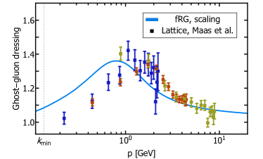
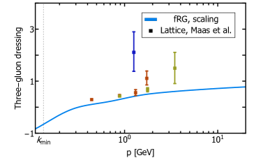
Figure 14: Transverse ghost-gluon and three-gluon dressings (blue lines) in comparison to $SU(2)$ lattice results [88, 89, 90] with $N=32^{4}$, $\beta=\{2.13,\,2.39,\,2.60\}$ and $a^{-1}=\{0.8\,\text{GeV},\,1.6\,\text{GeV},\,3.2\,\text{GeV}\}$ for the dark blue/rusty red/ocher points.

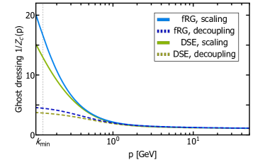
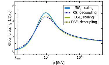
Figure 15: Ghost and gluon propagator dressings: Results from the fRG (blue) in comparison to the DSE [7] (green), for the scaling (solid) and decoupling (dashed) solution. The DSE dressings were rescaled such that they agree with the corresponding fRG dressings at $p=\Lambda=672.6\,$GeV.

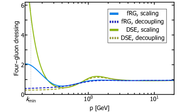
Figure 16: Gluon propagator and four-gluon dressing: Results from the fRG (blue) in comparison to the DSE [7] (green), for the scaling (solid) and decoupling (dashed) solution. The DSE dressings were rescaled such that they agree with the corresponding fRG dressings at $p=\Lambda=672.6\,$GeV.

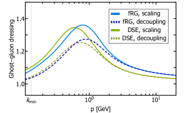
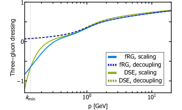
Figure 17: Transverse ghost-gluon and three-gluon dressings: Results from the fRG (blue) in comparison to the DSE [7] (green), for the scaling (solid) and decoupling (dashed) solution. The DSE dressings were rescaled such that they agree with the corresponding fRG dressings at $p=\Lambda=672.6\,$GeV.

A comparison of the transverse dressings from the fRG obtained from our setup to vertex dressings from lattice computations [88, 89, 90] and to DSE dressings from [7] are depicted in Appendix B in Figure 14, Figure 15, Figure 16 and Figure 17.

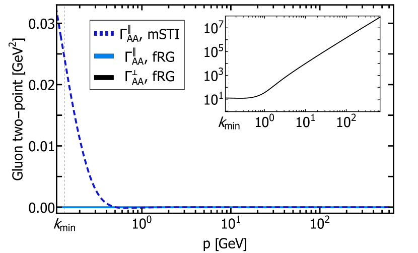
(a) Gluon two-point function.

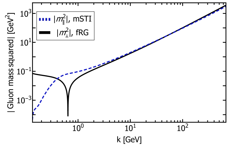
(b) Absolute value of effective gluon mass squared.

Figure 7: The gluon two-point function (7(a)) as a function of momentum $p$ and the corresponding effective mass (7(b)) as a function of RG-scale $k$. Results from the fRG are shown as solid lines, while mSTI results are shown as dashed lines. The transverse component is black and the longitudinal ones are depicted in blue. Please note that the transverse two-point function is only displayed in the inset.

III.2 Longitudinal & BRST correlation functions

The BRST symmetric Yang-Mills action additionally contains source terms $Q_{i}$ coupled to the respective BRST transformations of the fields. These vertices are fully dressed, see Section II.3, and this dressing carries the non-trivial deformation of the classical BRST transformations in the quantised theory. Then (quantum) BRST symmetry, and thus the mSTIs, relate the longitudinal parts of vertex functions to themselves and the transverse parts, see 31.

Evidently, for a self-consistent check of the (m)STIs we also need to compute the longitudinal and BRST dressings from the fRG. The symbolic equations were also derived using QMeS-Derivation and are depicted in Figure 18 in the Appendix D. Again, the average momentum approximation at the symmetric point 27 was used to simplify the momentum-dependence of the vertex dressings.

Diagrammatically, the fRG equations of the transverse and longitudinal quantities are identical, the vertices contributing in the diagrams are however different. An illustrative and important example for these differences is given by the transverse and longitudinal gluon mass. In Section C.1 we derive the transverse and longitudinal one-loop effective gluon mass from the fRG and mSTI.

As a first application we discuss the three-gluon dressing with one longitudinal leg. It vanishes at the symmetric point,

$$\lambda_{A^{3},1}\propto\mathcal{P}^{abc}_{A^{3},1,\mu\nu\rho}(p,q)\Gamma_{A^{3},\mu\nu\rho}^{abc}(p,q) =0\,,$$ (39)

rendering this dressing RG-invariant, $\dot{\lambda}_{A^{3},1}=0$. We are led to

$$\lambda_{A^{3},1,k}(p)\equiv\lambda_{A^{3},1,\Lambda}\equiv\lambda_{A^{3},\Lambda}\,.$$ (40)

The same holds true for the three-gluon dressing with three longitudinal legs.

We use the same initial values for the longitudinal dressings as for the transverse ones. As the longitudinal gluon two-point function does not feed back into the flows, its initial value is chosen such that $\Gamma^{\parallel}_{AA,k_{\mathrm{min}}}(p)=0$.

The fine-tuning procedure described in Section III.1 also applies to the longitudinal sector: the initial values of the longitudinal dressings and of the longitudinal gluon mass at the cutoff have to be tuned such that they satisfy the respective STIs perturbatively at $k_{\text{min}}$. In this work, we refrain from tuning the longitudinal sector and rather choose regular vertices, where the initial values of the respective longitudinal and transverse vertex dressings agree. We thus expect a small deviation of the STIs for perturbative momenta. This deviation is directly related to the functional nature of the the mSTIs and the fRG equations that are solved within a truncation.

Longitudinal fRG equations are coupled to the transverse sector and to themselves, see Section II.4. In contrast to those in the transverse sector, the equations decouple hierarchically due to the non-running of the three-gluon vertex dressing with one longitudinal leg. Hence we can solve them successively. The projection procedure for the derivation of longitudinal fRG equations can be found in Section B.1.

The longitudinal system is solved self-consistently, the input being the transverse dressings. Moreover, we compute the longitudinal four-gluon dressings from the STI 49 as these relations are computationally far simpler accessible. They are depicted in Figure 5. The results for the longitudinal fRG dressings are shown in Figure 4 and Figure 7. A discussion is postponed to Section III.4.

We also compute the BRST dressings from the fRG. Here, shift symmetry allows for the identification of the $Z_{cQ_{A}}$, $\lambda_{AcQ_{A}}$ and $\lambda_{AcQ_{A},1}$ with the ghost and transverse and longitudinal ghost-gluon dressing, see Section B.6, thus one only has to compute the remaining dressing, $\lambda_{Q_{c}cc}$. Furthermore, we show in Section III.3.2 that this dressing is also related to the longitudinal ghost-gluon dressing.

III.3 Modified Slavnov-Taylor Identitites

In this section we insert the fRG results into the (m)STI equations and recompute longitudinal correlation functions. Hence, we solve the STIs within our truncation, which offers a non-trivial check of gauge consistency of our solution. A discussion and comparison of the correlation functions obtained from the fRG and from the mSTI can be found in Section III.4 and a comparison of thereof for different types of solutions is given in Section III.5.

For the derivation procedure and the diagrammatic contributions, see Appendix C. All (m)STIs are evaluated at the symmetric point 26 and the dressings are computed on the average momentum configuration 27.

Numerically, it is not feasible to integrate the equations down to $k=0$, and we keep a small, yet finite, cutoff $k_{\text{min}}=0.135\,$GeV. Consequently, we do not check the gauge consistency of our results with the STIs but rather with the mSTIs at $k=k_{\text{min}}$. In the following we will refer to expressions of the general form

$$\textrm{STI $-$ Diagrams}\overset{!}{=}0\,,$$ (41)

as mSTIs. In 41, Diagrams stands for the one-loop diagrammatic corrections of the STI due to the BRST symmetry breaking cutoff terms 11. The symbolic equations are depicted in Appendix D in Figure 19.

As briefly discussed before, the mSTIs carry the underlying gauge invariance of the theory. Hence, the offer non-trivial gauge consistency checks of the correlation functions of a specific solution (e.g. scaling, decoupling or Higgs-type) of the theory obtained numerically within a truncation. Deviations of the mSTIs can be traced back to three sources: numerical precision, the truncation, and the chosen solution.

The first can be further split into infrared cutoff effects, that might break the mSTIs for momenta around the IR cutoff scale, $p\approx k_{\text{min}}$ and overall numerical precision. Accordingly, a quantitative check of the mSTIs is only possible at momentum scales, that are at least one order of magnitude larger than the cutoff $k_{\text{min}}$.

Truncation artefacts manifest themselves in a twofold way: effects related to dropped vertices and sub-leading tensor structures should only result in a deviation in the infrared and the semi-perturbative regime, $p\ll 5\,$GeV.

Nonetheless, even the most sophisticated truncation in the fRG does not lead to correlation functions that fully satisfy the mSTIs: both constitute different resummations and can only agree within approximations that lead to the same full resummations in both classes of functional equations. Thus, one expects an overall deviation of the mSTIs on all momentum scales. Lastly, deviations in the mSTIs might occur due to the chosen solution of Yang-Mills theory, i.e. the scaling, the decoupling or a Higgs-type solution. Generally, we expect the mSTIs to be best fulfilled by the true scaling solution. Moving away from that (along the x-axis in Figure 6) deviations of the mSTIs should occur at larger and larger momentum scales.

This entails, that an interpretation of the mSTI results is a difficult task as a clear disentanglement of all of the mentioned sources necessitates further computations of the different types of solutions within different truncations, and with different IR cutoffs and numerical precision.

III.3.1 Gluon Two-Point and Gluon Mass STI

The STI for the longitudinal gluon two-point function is simply given by vanishing quantum corrections of the longitudinal two-point function,

$$\Gamma^{\parallel}_{AA,\text{reg}}(p)=0\,,$$ (42)

where the full longitudinal gluon two-point function consists out of the loop contribution $\Gamma^{\parallel}_{AA,\text{reg}}$ and the gauge fixing, see 16. This also implies a vanishing longitudinal gluon mass,

$$m_{\parallel}^{2}=\Gamma^{\parallel}_{AA}(p=0)=0\,.$$ (43)

Both, the full longitudinal gluon two-point function $\Gamma^{\parallel}_{AA}(p)$ and the longitudinal gluon mass $m_{\parallel}^{2}$ are depicted in Figure 7. In Figure 8 we depict the the deviation of the two-point function mSTI as defined in 41, the cutoff dependence of transverse (fRG) and longitudinal (mSTI) masses is depicted in Figure 7. Technical details can be found in Section B.3. A discussion of these findings is deferred to Section III.4.

Figure 8: Absolute value of the gluon two-point mSTI as a function of momentum $p$ for different values of $k$.

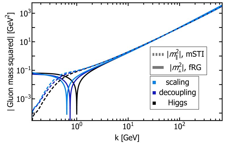
(a) Absolute value of individual contributions. fRG results are shown with solid lines and mSTI results with dashed lines.

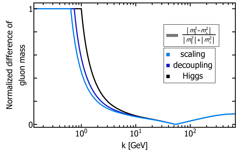
(b) Normalized difference.

Figure 9: Comparison of the flow of the effective transverse (fRG) and longitudinal gluon mass (mSTI) as a function of the cutoff scale $k$. The transverse part is taken from the fRG. The colors differentiate the different solutions (scaling, decoupling, Higgs-type).

III.3.2 Ghost-Gluon STI

The STI for the ghost-gluon vertex relates the longitudinal part of ghost-gluon vertex to the BRST projected vertex $Q_{c}cc$. In our truncation we are led to

$$2p_{\mu}\Gamma_{A\bar{c}c,\mu}(p,q)Z_{c}(p)+q^{2}\Gamma_{ccQ_{c}}(p,-p-q)Z_{c}(q)=0\,.$$ (44)

Thus we can derive the STI for the respective dressings at the symmetric point,

$$\lambda_{A\bar{c}c,1}(p)-\lambda_{Q_{c}cc}(p)=0\,.$$ (45)

A formulation of the ghost-gluon STI in terms of the classical and non-classical tensor basis is presented in Section C.2. The respective dressings are depicted in Figure 4 and Figure 13.

III.3.3 Three-Gluon STI

The STI for the three-gluon vertex with two longitudinal legs at the symmetric point is given by,

$$\lambda_{A^{3},2}(p)-\frac{Z_{A}(p)}{Z_{c}(p)}\lambda_{Q_{c}cc}(p)=0\,.$$ (46)

After applying the symmetric point ghost-gluon STI in our truncation, 45, and dividing by propagator dressings, one obtains the relation for the couplings,

$$\frac{\lambda^{2}_{A^{3},2}(p)}{4\pi Z^{3}_{A}(p)}=\frac{\lambda^{2}_{A\bar{c}c,1}(p)}{4\pi Z_{A}(p)Z^{2}_{c}(p)}\,.$$ (47)

Using the ghost-gluon STI to simplifly the equation is a valid approximation as is shown in Section III.4.3 and Figure 10. Assuming regularity, i.e. agreement of transverse and longitudinal projections of correlation functions (at least for large momenta), the above relation is similar to the well-known perturbative relation presented in 29.

The dressings of the different longitudinal and transverse projection of the classical tensor structure of the three gluon vertex are shown in Figure 4. We remark, that no STI is obtained for the projection with two transverse and one longitudinal leg at the symmetric point, since this projection renders zero.

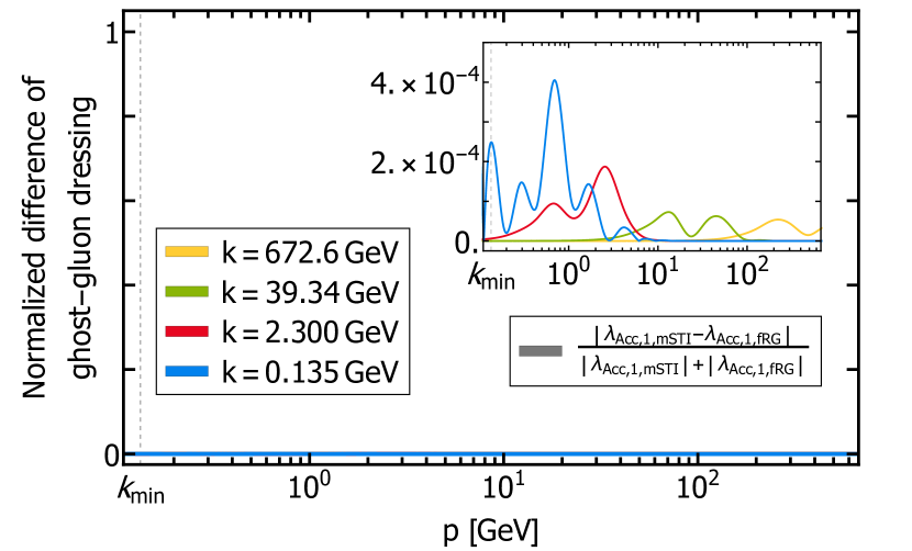
(a) Ghost-gluon vertex dressing. The result is numerically compatible with zero, which becomes evident in the inset.

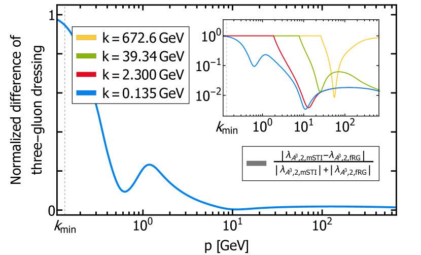
(b) Three-gluon vertex dressing. The difference gets maximal in the IR, a logarithmic version is shown in the inset.

Figure 10: Normalized difference of the longitudinal three-point dressings between the fRG and the mSTI at different RG-scales $k$ as a function of momentum $p$.

III.3.4 Four-Gluon STI

The four-gluon STI relates different longitudinal four-gluon dressings to longitudinal and transverse three-gluon and ghost-gluon dressings. We have again used the symmetric point ghost-gluon STI 45 and arrive at the four-gluon STIs at the symmetric point. The one for the four-gluon vertex with one longitudinal leg, $\lambda_{A^{4},1}(p)$, is given by,

$$\lambda_{A^{4},1}(p)-\frac{1}{Z_{c}(p)}\lambda_{A\bar{c}c}(\frac{\sqrt{10}}{3}p)\lambda_{A^{3}}(\frac{\sqrt{10}}{3}p)=0\,,$$ (48)

The STI for the four-gluon vertex with two longitudinal legs, $\lambda_{A^{4},2}(p)$, is given by,

$$\lambda_{A^{4},2}(p)-\frac{32}{33Z_{c}(p)}\lambda_{A\bar{c}c,1}\left(\frac{\sqrt{10}}{3}p\right)\lambda_{A^{3}}\left(\frac{\sqrt{10}}{3}p\right)$$

$$-\frac{1}{33Z_{c}(p)}\lambda_{A\bar{c}c}\left(\frac{\sqrt{10}}{3}p\right)\lambda_{A^{3},1}\left(\frac{\sqrt{10}}{3}p\right)=0\,,$$ (49)

It is worth mentioning that the momentum argument of the dressings in the STIs at the symmetric point are quite different from the ones usually present in the literature, as e.g. in 29. Using the STI for the three-gluon dressing, the STIs for the four-gluon dressing with one and two longitudinal legs are equivalent to the form in 29 assuming regularity of vertices for large momenta.

III.4 Discussion

We now compare the longitudinal results of different correlation functions obtained from the fRG and mSTI approach by studying the normalised difference of the respective quantities.

III.4.1 Longitudinal Gluon Mass

The longitudinal mSTI mass, $m^{2}_{\parallel}$, and the effective transverse fRG mass, $m^{2}_{\perp}$ exhibit the same running for large $k$ which is shown in Figure 7. This is in good agreement with the one-loop running, which is the same for both masses, for further details, see Section C.1. At about cutoff scales $k\approx 5\,$GeV, the two mass start deviating from each other. This is triggered by the difference in the IR of the longitudinal and transverse vertices, cf. Figure 4.

We remark, that the values of the longitudinal mSTI and transverse fRG masses are finite and approximately agree at $k_{\mathrm{min}}$, while the longitudinal fRG mass is zero. This is due to the regularity of the vertices in the present approximation at finite cutoff. In the scaling solution, irregular vertices emerge at $k\to 0$, while the decoupling solution does not incorporate the irregular vertices required for confinement in the current approximation. The STI, 43, however, renders the longitudinal gluon mass zero at $k=0$. Evidently, this deviation at least partially stems from our truncation in the vertex sector in the fRG equations, see also the discussion in Section III.4.2. To circumvent this discrepancy, we have extracted the longitudinal mSTI mass at $p=4\,k_{\textrm{min}}$, in order to avoid the influence of any IR cutoff effects that are present for $p\lesssim k_{\textrm{min}}$. For more details, see Section B.3.

III.4.2 Longitudinal Gluon Two-Point Function

The solution of the longitudinal two-point fRG equation constitutes the simplest case possible since it does not at all feed back into fRG diagrams in the Landau gauge. We also remark that the longitudinal propagator does feed back to the mSTI, but only its classical gauge fixing part. In summary this entails, that the longitudinal gluon two-point function is obtained by simply integrating the flow equation, and choosing the initial condition for $\Gamma^{\parallel}_{AA,\mu\nu,\text{reg},\Lambda}(p)$ such, that one obtains zero for the evaluated integral. This procedure not only solves the fRG equation but also satisfies the STI at $k_{\mathrm{min}}$, hence disregarding the small breaking of the STI for small momentum scales.

By comparing the longitudinal gluon two-point function from the fRG and from the mSTI, one can see that they do not agree well on all scales $k$, see Figure 7 and Figure 8. They are only identical at $k=k_{\mathrm{min}}$ for $p\gtrsim 0.5\,$GeV. For small momenta one can see a deviation of order $\mathcal{O}(10^{-2}\,\text{GeV}^{2})$. Albeit small, the deviation is qualitatively similar to the deviation in the three-gluon mSTI, Figure 10. Since the longitudinal three-gluon dressing enters the mSTI equation for the gluonic two-point function, but not vice versa, one can therefore conclude, that both deviations are due to the truncation of the fRG equation for the longitudinal three-gluon and four-gluon dressing.

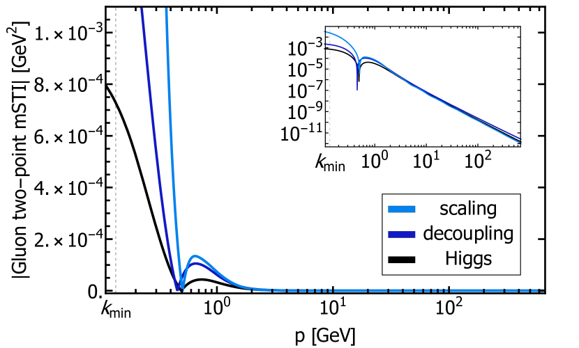
(a) Absolute value of gluon two-point STI. The inset shows a logarithmic scale.

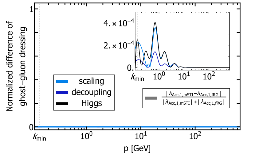
(b) Normalized difference of the ghost-gluon STI. The result is numerically compatible with zero, which is evident from the inset, where the full data range is displayed.

Figure 11: Results for the STI of the gluon two-point and the ghost-gluon vertex dressing as a function of momentum $p$. The colors differentiate IR scenarios.

III.4.3 Longitudinal Ghost-Gluon Dressing

In a general covariant gauge, only $\lambda_{A\bar{c}c}$ requires renormalisation. The non-classical dressing $\lambda_{A\bar{c}c,ncl}$ vanishes for large momenta. The non-classical dressing obtained from the fRG and mSTI is depicted in Figure 13.

We can see that our results fulfil this property perturbatively since the non-classical dressing is approximately zero for large momenta, $p\gg 5\,$GeV. In the infrared, it is however non-trivial. It is worth mentioning that the longitudinal and transverse ghost-gluon dressings do not agree well at any momentum scale $p$.

From Figure 4, Figure 10, and Figure 13 in the appendix, we can see that the mSTI and fRG dressing agree perfectly for all momenta $p$ implying that there is a non-trivial cancellation of diagrams within the two functional approaches. Indeed, Figure 10 merely depicts the numerical accuracy of our computation.

Generally, this non-trivial result implies BRST symmetry being conserved by the respective fRG computation and thus strongly hints at gauge consistency of our setup.

III.4.4 Longitudinal Three-Gluon Dressing

The results for the different three-gluon dressings are shown in Figure 4. As demonstrated in 39 the three-gluon dressing with one longitudinal leg, $\lambda_{A^{3},1}$, does not run. One can see that the dressing with two longitudinal legs from the fRG agrees with the transverse fRG dressing, $\lambda_{A^{3}}$, and the longitudinal STI dressing for large momenta $p\gg 5\,$GeV. The longitudinal STI dressing and the transverse fRG dressing however agree up to even smaller scales $p\gg 1.5\,$GeV.

In the infrared one can observe that the general behaviour of the longitudinal fRG and STI dressings agree. The STI dressing diverges for $p\rightarrow 0$ whereas the fRG dressing forms a maximum at $p\approx 0.2\,$GeV. The minimum of both dressings is given at approximately the same momentum, $p\approx 1\,$GeV.

In contrast to that, the transverse dressing gets smaller and even becomes negative for $p\rightarrow 0$. Thus we can observe a clear splitting between the transverse and longitudinal sector in both approaches which is due to the different contributions of longitudinal and transverse vertices in transverse and longitudinal functional equations.

The slight deviation in the UV can be explained by the logarithmic finetuning procedure: we have chosen the same initial values for the longitudinal and transverse dressings. The contributions on the level of correlation functions to the flows are however different. By choosing different (constant) initial values for the longitudinal dressings at the cutoff it is nevertheless possible to generate a better agreement of the dressings in the UV at $k=k_{\mathrm{min}}$.

As stated in the previous section, the three-gluon mSTI shows a deviation at $p\approx 5\,$GeV. This might be due to the fact that we did not include a full tensor basis of the gluonic sector and even approximated the longitudinal four-gluon dressings with their STI values in the fRG equation of the three-gluon vertex.

For momenta $p>5\,$GeV, the three-gluon mSTI is however fulfilled, where the small deviation for very large momenta stems from the tuning procedure, as described before.

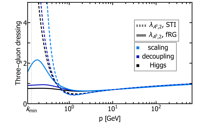
(a) Absolute value of individual contributions: fRG (solid lines), STI (dashed lines).

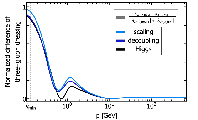
(b) Normalized difference.

Figure 12: Results for the longitudinal three-gluon dressing $\lambda_{A^{3},2}(p)$ as a function of the momentum $p$. The colors differentiate IR scenarios.

III.5 Discussion of Different Solutions

In this section, we present a comparison of the mSTIs for different types of solutions, i.e. the scaling, decoupling, and a Higgs-type solution, that are highlighted amongst the range of solutions in Figure 6.

Studying the normalized difference of the transverse andf longitudinal gluon mass, see Figure 9, where the longitudinal mass is obtained from the mSTI and the effective transverse mass from the fRG, one can see that all three solutions agree equally well up until $p\approx 20\,$GeV. There, the Higgs-type solution starts to deviate. It is expected that for a more massive Higgs-type solution, the deviation starts at an even larger momentum scale $p$. Vice versa, the scaling solution starts to deviate at a smaller scale than the decoupling solution.

The ghost-gluon mSTI is fulfilled for all three types of solutions, the small deviations shown in Figure 11 simply depict the numerical precision in the computation.

Generally, we do not expect the mSTIs to be fulfilled for scales $p\ll 1\,$GeV, since non-classical vertices and tensor structures that were not taken into account in our truncation, contribute significantly in this regime. We furthermore expect IR cutoff effects contributing below this scale, being within one order of magnitude of $k_{\mathrm{min}}$.

However, we can clearly see the expected divergence in the gluon two-point, Figure 11, and three-point mSTI, Figure 12, for momenta $p\ll 1\,$GeV.

Comparing the longitudinal three-gluon dressing $\lambda_{A^{3},2}$ from the fRG and from the STI for different types of solutions, one can see that the scaling solution yields the best qualitative agreement of the dressings.

IV Conclusion

We studied the gauge consistency of functional approaches to Yang-Mills within the Landau gauge. For this purpose, we resolved the transverse and longitudinal sector by solving the corresponding fRG flow equations for the dressings of transverse and longitudinal propagators and vertices in a sufficiently advanced truncation. To quantify the violation of gauge consistency in such a set-up, we also computed longitudinal dressings with the associated modified Slavnov-Taylor identities. The results agree within numerical accuracy for momentum scale $p\gtrsim 1\,\mathrm{GeV}$. We found that the agreement of STI dressings and fRG dressings differ for the solutions branches, i.e. for scaling, decoupling and Higgs type solutions: in general, the scaling solution shows the best agreement. In turn, the longitudinal fRG dressings for decoupling and Higgs-type solutions start to deviate from the ST dressings for successively larger momenta, the farer away they are from scaling. Interestingly, the longitudinal three-gluon vertex dressing is an exception, as there the deviation of fRG and STI dressings happens at roughly the same scale. This structure deserves further investigation, one of the reasons being that the STIs used in the present work are the standard Landau gauge STIs and the decoupling and Higgs-type solutions triggered here are effectively induced by an explicit mass parameter as in the Curci-Ferrari (CF) model. This suggests to repeat the present investigation on the basis of the CF BRST transformations.

In summary, these comparisons provide us with a tool to control the gauge consistency in truncations of the quantum effective action. In our opinion, the present level of gauge consistency supports the reliability of such truncations in applications of non-perturbative functional methods to Yang-Mills theory.

Monitoring the mSTIs in such a manner provides additional, much needed, guidance to improve on truncations. Alternatively, they can be used as constraints to determine correlation functions.

This work provides the foundation for an advanced study thereof in QCD, where the gauge consistency of the coupled self-consistent quark-gluon system poses an intricate problem. We hope to report on this in the near future.

Appendix A Numerical Implementation

The fRG and mSTI equations were derived using QMeS [4, 5], a Mathematica package for the derivation of symbolic functional equations. After projecting onto the respective tensor structures, the equations were traced with FormTracer [92, 93]. The resulting momentum-dependent integral-differential and integral equations were solved in Mathematica 12.0.

Appendix B Additional Details on the fRG Computation

B.1 Projecting onto Tensor Structures

On the level of two-point functions, we have two quantities that contribute to the transverse sector, the gluon and the ghost two-point function. Their tensor structures are,

$$\tau^{ab}_{AA,\mu\nu}(p) =\delta^{ab}\left(\Pi^{\perp}_{\mu\nu}(p)p^{2}+\Pi^{\parallel}_{\mu\nu}(p)p^{2}\right)\,,$$

$$\tau^{ab}_{c\bar{c}}(p) =-\delta^{ab}p^{2}\,.$$ (50)

For the derivation of their respective fRG equations we trace the diagrammatic equations with the projection operators,

$$\mathcal{P}^{ab}_{c\bar{c}}(p) =\tau_{c\bar{c}}^{ab}(p)\,,$$

$$\mathcal{P}^{\perp,ab}_{AA,\mu\nu}(p) =\Pi^{\perp}_{\mu\bar{\mu}}(p)\Pi^{\perp}_{\nu\bar{\nu}}(p)\tau^{ab}_{AA,\bar{\mu}\bar{\nu}}(p)\,,$$

$$\mathcal{P}^{\parallel,ab}_{AA,\mu\nu}(p) =\Pi^{\parallel}_{\mu\bar{\mu}}(p)\Pi^{\parallel}_{\nu\bar{\nu}}(p)\tau^{ab}_{AA,\bar{\mu}\bar{\nu}}(p)\,.$$ (51)

for the ghost and transverse gluon propagator dressing, and for the longitudinal gluon two-point respectively.

The tensor structures of the ghost-gluon vertex can be written as,

$$\tau^{abc}_{A\bar{c}c,\mu}(p,q) =if^{abc}\left(\Pi^{\perp}_{\mu\nu}(p)+\Pi^{\parallel}_{\mu\nu}(p)\right)q_{\nu}\,.$$ (52)

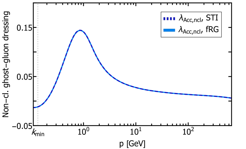
Figure 13: Non-classical ghost-gluon dressing from the fRG (solid blue) and STI (dashed dark blue).

The fRG equations for the transverse and longitidunal ghost-gluon dressing are obtained by contracting the equation from Figure 18 with,

$$\mathcal{P}^{abc}_{A\bar{c}c,\mu}(p,q) =\Pi^{\perp}_{\mu\bar{\mu}}(p)\tau^{abc}_{A\bar{c}c,\bar{\mu}}(p,q)\,,$$

$$\mathcal{P}^{\parallel,abc}_{A\bar{c}c,\mu}(p,q) =\Pi^{\parallel}_{\mu\bar{\mu}}(p)\tau^{abc}_{A\bar{c}c,\bar{\mu}}(p,q)\,.$$ (53)

From the longitudinal and transverse/classical ghost-gluon dressing one can compute the non-classical vertex dressing 20. The result is shown in Figure 13. One can see that it is approximately zero for perturbative momenta.

As a tensor basis for the three- and four-gluon vertex, we apply transverse and longitudinal projections of the classical tensor structures,

$$\tau_{A^{3},\text{cl},\mu\nu\rho}^{abc}(p,q)=-if^{abc}$$

$$\left(\delta_{\mu\nu}(p-q)_{\rho}+\delta_{\nu\rho}(2q+p)+\delta_{\rho\mu}(-2p-q)\right)\,,$$ (54)

and

$$\tau_{A^{4},\text{cl},\mu\nu\rho\sigma}^{abcd}(p,q,r) =f^{abe}f^{cde}\left(\delta_{\mu\rho}\delta_{\nu\sigma}-\delta_{\mu\sigma}\delta_{\nu\rho}\right)$$

$$+f^{ace}f^{bde}\left(\delta_{\mu\nu}\delta_{\rho\sigma}-\delta_{\mu\sigma}\delta_{\nu\rho}\right)$$

$$+f^{ade}f^{bce}\left(\delta_{\mu\nu}\delta_{\rho\sigma}-\delta_{\mu\rho}\delta_{\nu\sigma}\right)\,.$$ (55)

We obtain the transverse and longitudinal three- and four-gluon vertex dressings by contracting the full vertices with the transverse longitudinal projection operators 15 applied to the classical tensor structures. The resulting projection operators are,

$$\mathcal{P}^{abc}_{A^{3},\mu\nu\rho}(p,q)= \Pi^{\perp}_{\mu\bar{\mu}}(p)\Pi^{\perp}_{\nu\bar{\nu}}(q)\Pi^{\perp}_{\rho\bar{\rho}}(-p-q)$$

$$\tau_{A^{3},\text{cl},\bar{\mu}\bar{\nu}\bar{\rho}}^{abc}(p,q)\,,$$

$$\mathcal{P}^{abc}_{A^{3},1,\mu\nu\rho}(p,q)= \Pi^{\perp}_{\mu\bar{\mu}}(p)\Pi^{\perp}_{\nu\bar{\nu}}(q)\Pi^{\parallel}_{\rho\bar{\rho}}(-p-q)$$

$$\tau_{A^{3},\text{cl},\bar{\mu}\bar{\nu}\bar{\rho}}^{abc}(p,q)\,,$$

$$\mathcal{P}^{abc}_{A^{3},2,\mu\nu\rho}(p,q)= \Pi^{\perp}_{\mu\bar{\mu}}(p)\Pi^{\parallel}_{\nu\bar{\nu}}(q)\Pi^{\parallel}_{\rho\bar{\rho}}(-p-q)$$

$$\tau_{A^{3},\text{cl},\bar{\mu}\bar{\nu}\bar{\rho}}^{abc}(p,q)\,,$$ (56)

and,

$$\mathcal{P}^{abcd}_{A^{4},\mu\nu\rho\sigma}(p,q,r)=\Pi^{\perp}_{\mu\bar{\mu}}(p)\Pi^{\perp}_{\nu\bar{\nu}}(q)\Pi^{\perp}_{\rho\bar{\rho}}(r)$$

$$\Pi^{\perp}_{\sigma\bar{\sigma}}(-p-q-r)\tau_{A^{4},\text{cl},\bar{\mu}\bar{\nu}\bar{\rho}\bar{\sigma}}^{abcd}(p,q,r)\,,$$

$$\mathcal{P}^{abcd}_{A^{4},1,\mu\nu\rho\sigma}(p,q,r)=\Pi^{\perp}_{\mu\bar{\mu}}(p)\Pi^{\perp}_{\nu\bar{\nu}}(q)\Pi^{\perp}_{\rho\bar{\rho}}(r)$$

$$\Pi^{\parallel}_{\sigma\bar{\sigma}}(-p-q-r)\tau_{A^{4},\text{cl},\bar{\mu}\bar{\nu}\bar{\rho}\bar{\sigma}}^{abcd}(p,q,r)\,,$$

$$\mathcal{P}^{abcd}_{A^{4},2,\mu\nu\rho\sigma}(p,q,r)=\Pi^{\perp}_{\mu\bar{\mu}}(p)\Pi^{\perp}_{\nu\bar{\nu}}(q)\Pi^{\parallel}_{\rho\bar{\rho}}(r)$$

$$\Pi^{\parallel}_{\sigma\bar{\sigma}}(-p-q-r)\tau_{A^{4},\text{cl},\bar{\mu}\bar{\nu}\bar{\rho}\bar{\sigma}}^{abcd}(p,q,r)\,.$$ (57)

The tensor structures of the BRST-projected two-point vertices are given as,

$$\tau^{ab}_{AQ_{\bar{c}},\mu}(p)=-i\frac{p_{\mu}}{\xi}\delta^{ab}\,,$$

$$\tau^{ab}_{cQ_{A},\mu}(p)=-ip_{\mu}\delta^{ab}\,,$$ (58)

and of the BRST three-point functions as,

$$\tau^{abc}_{ccQ_{c}}(p,q)= -f^{abc}\,,$$

$$\tau^{abc}_{AcQ_{A},\mu\nu}(p,q)= -f^{abc}\left(\Pi^{\perp}_{\mu\nu}(p)+\Pi^{\parallel}_{\mu\nu}(p)\right)\,.$$ (59)

Analogously, we can construct the respective projection operators,

$$\mathcal{P}^{ab}_{AQ_{\bar{c}},\mu}(p)=\tau^{ab}_{AQ_{\bar{c}},\mu}(p)\,,$$

$$\mathcal{P}^{ab}_{cQ_{A},\mu}(p)=\tau^{ab}_{cQ_{A},\mu}(p)\,,$$ (60)

and,

$$\mathcal{P}^{abc}_{ccQ_{c}}(p,q)= \tau^{abc}_{ccQ_{c}}(p,q)\,,$$

$$\mathcal{P}^{abc}_{AcQ_{A},\mu\nu}(p,q)= \Pi^{\perp}_{\mu\bar{\mu}}(p)\tau^{abc}_{AcQ_{A},\bar{\mu}\nu}(p,q)\,,$$

$$\mathcal{P}^{abc}_{AcQ_{A},1,\mu\nu}(p,q)= \Pi^{\parallel}_{\mu\bar{\mu}}(p)\tau^{abc}_{AcQ_{A},\bar{\mu}\nu}(p,q)\,.$$ (61)

The relation between these tensor structures and the pure Yang-Mills ones is further elaborated in Section B.6.

B.2 Tuning of Initial Parameters

The constant initial conditions for the dressings and the transverse gluon mass at the UV cut-off scale $\Lambda=672.6\,\text{GeV}$ for our approximation of the scaling solution were chosen as,

$$\lambda_{A\bar{c}c,\Lambda} =\lambda_{A\bar{c}c,1,\Lambda}=\lambda_{Q_{c}cc,\Lambda}=1$$

$$\lambda_{A^{3},\Lambda} =\lambda_{A^{3},1,\Lambda}=\lambda_{A^{3},2,\Lambda}=0.981$$

$$\lambda_{A^{4},\Lambda} =0.981$$

$$m^{2}_{\perp,\Lambda} =-3708.5272\,\text{GeV}^{2}\,.$$ (62)

B.3 Regulators and Gluon Mass

The transverse gluon dressing $Z_{A}(p)$ contains the gluon mass gap and thus diverges below $\sim 1\,$GeV for $k\rightarrow 0$. For the numerical computations we parameterize the gluon two-point function as,

$$\Gamma^{ab}_{AA,\mu\nu}(p)= \,\Pi^{\perp}_{\mu\nu}(p)\,Z_{T}(p)\left(p^{2}+m_{T}^{2}\right)\,\delta^{ab}$$

$$\hskip 28.45274pt+\Pi^{\parallel}_{\mu\nu}(p)\Gamma^{\parallel}_{AA}(p)\,\delta^{ab}\,,$$ (63)

where the longitudinal part $\Gamma^{\parallel}_{AA}$ contains the gauge fixing term $p^{2}/\xi$. We obtain the effective transverse and longitudinal gluon mass from,

$$m_{\perp,k}^{2}=Z_{T}(0)\,m_{T}^{2}\,,\qquad m_{\parallel,k}^{2}=\Gamma^{\parallel}_{AA,k}(0)\,.$$ (64)

The longitudinal gluon mass from the mSTI however is extracted from,

$$m_{\parallel,k,\text{mSTI}}^{2}=\Gamma^{\parallel}_{AA,k,\text{mSTI}}(p=4k_{\mathrm{min}})\,,$$ (65)

where the minimal momentum was chosen sufficiently large to avoid any IR cutoff effects.

The effective parameter for the true scaling mass was extracted by extrapolation of $m^{2}_{\perp,\mathrm{kmin}}(m^{2}_{\perp,\Lambda})$. Since we are dealing with scaling, the relation between the effective mass and the UV mass parameter follows

$$m^{2}_{\perp,\mathrm{kmin}}=x_{0}\,(m^{2}_{\perp,\Lambda}-m^{2}_{\mathrm{ref}})^{\alpha}\,.$$ (66)

Fitting the six left most values, we obtain

$$x_{0} =1.08\cdot 10^{-4}$$

$$\alpha =-0.097$$

$$m^{2}_{\mathrm{ref}} =-0.00812\Lambda^{2}=1.15\,m^{2}_{\perp,\Lambda,\,\text{1-loop}}\,,$$ (67)

with the one-loop mass defined in 83.

For the ghost and gluon regulator we use respectively,

$$(R_{A})^{ab}_{\mu\nu}(p)= \,\delta^{ab}r(p^{2}/k^{2})$$

$$\left(\Pi^{\perp}_{\mu\nu}(p)\bar{Z}_{T}(p)\,p^{2}+\Pi^{\parallel}_{\mu\nu}(p)\Gamma^{\parallel}_{AA}(p)\right)\,,$$

$$(R_{c})^{ab}(p) =\delta^{ab}p^{2}Z_{c}(p)r(p^{2}/k^{2})\,,$$ (68)

where k is the RG scale and we parametrise the transverse gluon two-point as,

$$\Gamma_{AA,\mu\nu}^{\perp,ab}(p) =\Pi_{\mu\nu}^{\perp}(p)Z_{T}(p)(p^{2}+m_{T}^{2})\delta^{ab}$$ (69)

$$=\Pi_{\mu\nu}^{\perp}(p)\left(\bar{Z}_{T}(p)(p^{2}+\bar{m}_{T}^{2}+k^{2})-k^{2}\right)\delta^{ab}\,.$$

The dressing $\bar{Z}_{T}$ guarantees a well-defined regulator in the infrared. The shape function is defined as an exponential,

$$r(p^{2}/k^{2})=\frac{e^{-p^{2}/k^{2}}}{1-e^{-p^{2}/k^{2}}}\,.$$ (70)

B.4 Extraction of Scale

We set the momentum scale by positioning the maximum of the gluon dressing $1/Z_{A}(p)$ at the lattice scale $p\approx 0.955\,$GeV from [47].

When comparing our propagators and dressings to the aforementioned lattice results one also has to adjust the global normalisation, $Z_{\text{Lat}}^{-1}(p)\rightarrow yZ_{\text{Lat}}^{-1}(p)$. This is done via minimizing

$$N_{Z_{A}}(y)=\sum_{i}\frac{\Delta x_{i}}{\Delta E_{i}^{2}}\left[\left(Z_{A}^{-1}(p_{i})-yZ_{\text{Lat}}^{-1}(p_{i})\right)^{2}\right.$$

$$\left.+\left(\partial_{p}Z_{A}^{-1}(p_{i})-y\partial_{p}Z_{\text{Lat}}^{-1}(p_{i})\right)^{2}\right]$$ (71)

in the region $0.8\,$GeV$\,\leq p_{i}\leq 4\,$GeV, where the lattice input $\Delta x_{i}$ denotes the distances to the next point, $\Delta E_{i}^{2}$ the statistical error of that point and $Z_{\text{Lat}}^{-1}(p)$ is the gluon dressing obtained from the respective lattice computation [47] and [58]. The normalisation procedure for the ghost dressing is done analogously in the fitting range $1.5\,$GeV$\,\leq p_{i}\leq 6\,$GeV.

B.5 Scaling Exponents

The scaling exponents, c.f. 37, obtained from our transverse scaling results in the regime $0.135\,$GeV$\,\leq p\leq 0.471\,$GeV are

$$\kappa_{gl}=0.535$$

$$\kappa_{gh}=0.541$$ (72)

B.6 BRST Projected Vertices

The effective action exhibits shift symmetry in the anti-ghost. This symmetry leads to the identities,

$$\partial\cdot\frac{\delta\Gamma}{\delta Q_{A}} =\frac{\delta\Gamma}{\delta\bar{c}}\,,$$

$$\frac{\delta\Gamma}{\delta Q_{\bar{c}}} =\frac{1}{\xi}\partial\cdot A\,.$$ (73)

Fourier transforming both gives,

$$-iq_{\nu}\Gamma_{Q_{A},\nu}(q) =\Gamma_{\bar{c}}(q)\,,$$

$$\Gamma_{Q_{\bar{c}}}(-p) =\frac{1}{\xi}ip_{\mu}A_{\mu}(p)\,.$$ (74)

The first identity relates,

$$iq_{\nu}\Gamma^{adb}_{AcQ_{A},\mu\nu}(p,-p-q) =\Gamma^{abd}_{A\bar{c}c,\mu}(p,q)\,,$$

$$ip_{\mu}\Gamma^{ba}_{cQ_{A},\mu}(-p) =\Gamma^{ab}_{\bar{c}c}(p)\,.$$ (75)

Generally we can write down the full tensor basis,

$$\Gamma^{adb}_{AcQ_{A},\mu\nu}(p,-p-q)= f^{abd}\left(\delta_{\mu\nu}\lambda_{1}+p_{\mu}p_{\nu}\lambda_{2}+q_{\mu}q_{\nu}\lambda_{3}\right.$$

$$\left.+p_{\mu}q_{\nu}\lambda_{4}+q_{\mu}p_{\nu}\lambda_{5}\right)\,.$$ (76)

The shift symmetry identity 75 then relates,

$$\lambda_{A\bar{c}c}= \,\lambda_{1}+q^{2}\lambda_{3}+pq\lambda_{5}$$

$$\lambda_{A\bar{c}c,ncl}= \,pq\lambda_{2}+q^{2}\lambda_{4}$$

$$\lambda_{A\bar{c}c,\parallel}= \,\lambda_{1}+q^{2}\lambda_{3}+pq\lambda_{5}$$

$$-2pq\lambda_{2}-2q^{2}\lambda_{4}\,.$$ (77)

The diagrams contributing to the flow of the $AcQ_{A}$- and $cQ_{A}$-dressings are depicted in Figure 18. One can see that the identity 75 is already diagrammatically fulfilled for the fRG equations. Thus they are exact identities. Therefore applying them in the STIs is valid and the exactness of the identities guarantees gauge parameter independence of the three-gluon STI. However the STIs not only depend on these specific combinations of dressings, therefore a computation of all five from the fRG is nonetheless necessary.

We however simplify the approximation by identifying,

$$\lambda_{AcQ_{A},1}(p,-p-q) =\lambda_{A\bar{c}c,1}(p,q)\,,$$

$$\lambda_{AcQ_{A}}(p,-p-q) =\lambda_{A\bar{c}c}(p,q)\,,$$

$$Z_{cQ_{A}}(p) =Z_{c}(p)\,,$$ (78)

where the index $1$ indicates a longitudinally projected gluon. This approximation should not lead to qualitative differences.

Appendix C Additional Details on the mSTI

C.1 Longitudinal Gluon Two-Point Function and Gluon Mass

To obtain the mSTI of the longitudinal gluon two-point function one takes the functional derivatives $\delta^{2}/(\delta A_{\mu}^{a}\delta c^{b})$ of the mSTI 11 projects both sides of the equation with,

$$\mathcal{Q}^{ab}_{AA,\mu}=p_{\nu}\tau^{ab}_{AA,\nu\mu}(p)\,.$$ (79)

After normalisation, one obtains the STI

$$\Gamma^{\parallel}_{AA,\text{reg}}(p)=0\,.$$ (80)

We can compare the effective one-loop, transverse and longitudinal, mass running from the fRG with the one-loop longitudinal mass from the STI. The different diagrams contributing to the equations are depicted in Figure 18 and Figure 19. Inserting undressed propagators and vertices with a gauge coupling $g$ and the regulator shape function $r(q^{2})\equiv r(q^{2}/k^{2})$, see 70, one obtains for the effective transverse gluon mass from the fRG,

$$\dot{m}^{2}_{\perp,\text{1-loop}}=\int dz\,dq\, \frac{q^{3}\sqrt{1-z^{2}}}{4\pi^{3}}\frac{g^{2}q^{2}\dot{r}(q^{2})}{q^{4}(1+r(q^{2}))^{3}}$$

$$\left(3-9z^{2}+r(q^{2})(-7+z^{2})\right)$$ (81)

where $z=\frac{p\cdot q}{\left|p\right|\left|q\right|}$. Performing the loop integration, one arrives at the one-loop running,

$$\dot{m}^{2}_{\perp,\text{1-loop}}=k\partial_{k}m^{2}_{\perp}=-\frac{9g^{2}}{64\pi^{2}}k^{2}\,.$$ (82)

Solving the differential equation yields,

$$m^{2}_{\perp,\text{1-loop}}=-\frac{9g^{2}}{128\pi^{2}}k^{2}\,.$$ (83)

For the longitudinal gluon mass from the fRG one obtains,

$$\dot{m}^{2}_{\parallel,\text{1-loop}}=\int dzdq \frac{q^{3}\sqrt{1-z^{2}}}{4\pi^{3}}\frac{g^{2}q^{2}\dot{r}(q^{2})}{q^{4}(1+r(q^{2}))^{3}}$$

$$\left(2-9z^{2}+r(q^{2})(2+z^{2})\right)\,.$$ (84)

Even though the longitudinal vertices contribute differently, one arrives at the same one-loop running as for the effective transverse mass and thus the longitudinal mass is,

$$m^{2}_{\parallel,\text{1-loop}}=-\frac{9g^{2}}{128\pi^{2}}k^{2}\,.$$ (85)

For the derivation of the one-loop mass from the mSTI, one has to take the zero momentum limit $p\rightarrow 0$ of the equation for $\Gamma^{AA}_{\parallel}(p)$ with the rule of l’Hospital,

$$\lim\limits_{p\rightarrow 0}\frac{f(p)}{g(p)}=\lim\limits_{p\rightarrow 0}\frac{f^{\prime}(p)}{g^{\prime}(p)}\,.$$ (86)

One then obtains the equation,

$$m^{2}_{\parallel,\text{1-loop}}= \int dzdq\frac{q^{3}\sqrt{1-z^{2}}}{4\pi^{3}}\frac{g^{2}q^{2}r(q^{2})}{q^{4}(1+r(q^{2}))^{3}}$$

$$\left((-2+9z^{2})(1+r(q^{2}))+8q^{2}z^{2}\partial_{q}r(q^{2})\right)\,.$$ (87)

Integrating this, one arrives at the same one-loop mass as from the fRG,

$$m^{2}_{\parallel,\text{1-loop}}=-\frac{9g^{2}}{128\pi^{2}}k^{2}\,.$$ (88)

Although all three equations contain different contributions and diagrams, they yield the same effective gluonic mass at one-loop level.

C.2 Ghost-Gluon Vertex mSTI

We take the functional derivatives $\delta^{3}/(\delta\bar{c}^{a}\delta c^{b}\delta c^{c})$ of 11. To project onto the dressings we trace the equation with $f^{abc}$. Thus the projection operator is,

$$\mathcal{Q}^{abc}_{A\bar{c}c}(p,q)=p_{\mu}\tau^{abc}_{A\bar{c}c,\mu}(p,q)\,.$$ (89)

After normalisation, the STI for the non-classical ghost-gluon dressing at the symmetric point is given as,

$$\lambda_{Q_{c}cc}(p)-\lambda_{A\bar{c}c}(p)+2\lambda_{A\bar{c}c,noncl}(p)=0\,.$$ (90)

From this we can derive:

$$\lambda_{A\bar{c}c,ncl}(p) =\frac{1}{2}\left(\lambda_{A\bar{c}c}(p)-\lambda_{Q_{c}cc}(p)\right)\,,$$

$$\lambda_{A\bar{c}c}(p) =\lambda_{A\bar{c}c}(p)\,,$$

$$\lambda_{A\bar{c}c,1}(p) =\lambda_{A\bar{c}c}(p)-2\lambda_{A\bar{c}c,ncl}(p)=\lambda_{Q_{c}cc}(p)\,.$$ (91)

A comparison of the non-classical ghost-gluon dressing from the mSTI and from the fRG is shown in Figure 13.

C.3 Three-Gluon Vertex mSTI

One can derive the three-gluon mSTI by taking the functional derivatives $\frac{\delta^{3}}{\delta A_{\mu}^{a}\delta A_{\nu}^{b}\delta c^{c}}$. For the projection onto the mSTI for the three-gluon dressings with one and two longitudinal legs, $\lambda_{A^{3},1}(p)$ and $\lambda_{AAA,2}(p)$, one uses,

$$\mathcal{Q}^{abc}_{A^{3},1,\mu\nu}(p,q)= \,\Pi^{\perp}_{\mu\bar{\mu}}(p)\Pi^{\perp}_{\nu\bar{\nu}}(q)(-p-q)_{\bar{\rho}}$$

$$\tau^{abc}_{A^{3},cl,\bar{\mu}\bar{\nu}\bar{\rho}}(p,q)\,,$$

$$\mathcal{Q}^{abc}_{A^{3},2,\mu\nu}(p,q)= \,\Pi^{\perp}_{\mu\bar{\mu}}(p)\Pi^{\parallel}_{\nu\bar{\nu}}(q)(-p-q)_{\bar{\rho}}$$

$$\tau^{abc}_{A^{3},cl,\bar{\mu}\bar{\nu}\bar{\rho}}(p,q)\,.$$ (92)

Since the classical tensor structure has no overlap with the first projection operator, there exists no mSTI for $\lambda_{A^{3},1}(p)$ in our truncation, see also 39, for the equivalent case in the fRG equations.

C.4 Four-Gluon Vertex mSTI

We take the field derivatives $\frac{\delta^{3}}{\delta A^{a}_{\mu}(p4)A^{b}_{\nu}(p3)A^{c}_{\rho}(p2)}\frac{\delta}{\delta c^{d}(p1)}$ of 11. The projection operators to obtain mSTI equations for the longitudinal four-gluon dressings $\lambda_{A^{4},1}(p)$ and $\lambda_{A^{4},2}(p)$ are given as,

$$\mathcal{Q}^{abcd}_{A^{4},1,\mu\nu\rho}(p,q,r)=\Pi^{\perp}_{\mu\bar{\mu}}(p)\Pi^{\perp}_{\nu\bar{\nu}}(q)\Pi^{\perp}_{\rho\bar{\rho}}(r)$$

$$(-p-q-r)_{\bar{\sigma}}\tau^{abcd}_{A^{4},cl,\bar{\mu}\bar{\nu}\bar{\rho}\bar{\sigma}}(p,q,r)\,,$$

$$\mathcal{Q}^{abcd}_{A^{4},2,\mu\nu\rho}(p,q,r)=\Pi^{\perp}_{\mu\bar{\mu}}(p)\Pi^{\perp}_{\nu\bar{\nu}}(q)\Pi^{\parallel}_{\rho\bar{\rho}}(r)$$

$$(-p-q-r)_{\bar{\sigma}}\tau^{abcd}_{A^{4},cl,\bar{\mu}\bar{\nu}\bar{\rho}\bar{\sigma}}(p,q,r)\,.$$ (93)

Appendix D Diagrammatic mSTIs and fRG Equations

The diagrammatic fRG equations and mSTIs within the truncation that was used throughout this work are depicted in Figure 18 and Figure 19.

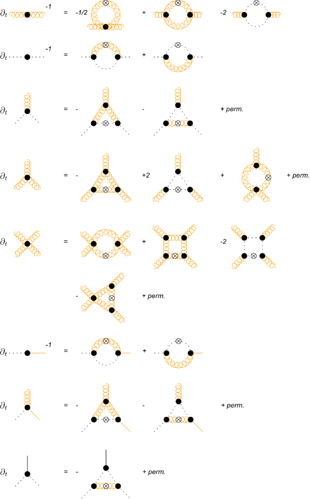
Figure 18: Diagrammatic representation of the flow equations of propagators and vertices. The dashed lines represent the fully dressed ghost, curly orange lines the fully dressed gluon, solid black lines to fully dressed $Q_{c}$ and solid orange lines to the fully dressed $Q_{A}$ BRST charge. The permutations include permutations of external legs as well as the position of the regulator derivative insertions which is indicated by the crossed circle. The power $-1$ indicates a full two-point function.

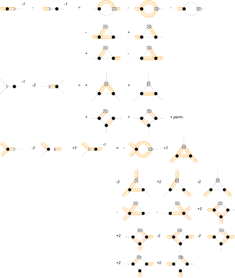
Figure 19: Diagrammatic representation of the modified Slavnov-Taylor identities for the longitudinal vertices. The dashed lines represent the fully dressed ghost, curly orange lines the fully dressed gluon. The black circles represent full vertices and the crossed square corresponds to a regulator and the triangle to a BRST vertex. The power $-1$ indicates a full two-point function. The permutations include permutations of external ghost legs.

References

- Fischer [2019] C. S. Fischer, QCD at finite temperature and chemical potential from Dyson–Schwinger equations, Prog. Part. Nucl. Phys. 105, 1 (2019), arXiv:1810.12938 [hep-ph] .
- Dupuis et al. [2021] N. Dupuis, L. Canet, A. Eichhorn, W. Metzner, J. M. Pawlowski, M. Tissier, and N. Wschebor, The nonperturbative functional renormalization group and its applications, Phys. Rept. 910, 1 (2021), arXiv:2006.04853 [cond-mat.stat-mech] .
- Fischer et al. [2009] C. S. Fischer, A. Maas, and J. M. Pawlowski, On the infrared behavior of Landau gauge Yang-Mills theory, Annals Phys. 324, 2408 (2009), arXiv:0810.1987 [hep-ph] .
- Pawlowski et al. [2021a] J. M. Pawlowski, C. S. Schneider, and N. Wink, QMeS-Derivation: Mathematica package for the symbolic derivation of functional equations, (2021a), arXiv:2102.01410 [hep-ph] .
- Pawlowski et al. [2021b] J. M. Pawlowski, C. S. Schneider, and N. Wink, QMeS-Derivation GitHub Repository (2021b), https://github.com/QMeS-toolbox/QMeS-Derivation.
- Cyrol et al. [2016a] A. K. Cyrol, L. Fister, M. Mitter, J. M. Pawlowski, and N. Strodthoff, Landau gauge Yang-Mills correlation functions, Phys. Rev. D 94, 054005 (2016a), arXiv:1605.01856 [hep-ph] .
- Huber [2020a] M. Q. Huber, Correlation functions of Landau gauge Yang-Mills theory, Phys. Rev. D 101, 114009 (2020a), arXiv:2003.13703 [hep-ph] .
- Corell et al. [2018] L. Corell, A. K. Cyrol, M. Mitter, J. M. Pawlowski, and N. Strodthoff, Correlation functions of three-dimensional Yang-Mills theory from the FRG, SciPost Phys. 5, 066 (2018), arXiv:1803.10092 [hep-ph] .
- Becchi et al. [1976] C. Becchi, A. Rouet, and R. Stora, Renormalization of Gauge Theories, Annals Phys. 98, 287 (1976).
- Tyutin [1975] I. V. Tyutin, Gauge Invariance in Field Theory and Statistical Physics in Operator Formalism, (1975), arXiv:0812.0580 [hep-th] .
- [11] J. M. Pawlowski, J. A. Bonnet, S. Rechenberger, M. Reichert, and N. Wink, -the functional renormalization group- & applications to gauge theories and gravity, (in preparation).
- Litim and Pawlowski [1998] D. F. Litim and J. M. Pawlowski, On gauge invariant Wilsonian flows, in Workshop on the Exact Renormalization Group (1998) pp. 168–185, arXiv:hep-th/9901063 .
- Berges et al. [2002] J. Berges, N. Tetradis, and C. Wetterich, Nonperturbative renormalization flow in quantum field theory and statistical physics, Phys. Rept. 363, 223 (2002), arXiv:hep-ph/0005122 .
- Pawlowski [2007] J. M. Pawlowski, Aspects of the functional renormalisation group, Annals Phys. 322, 2831 (2007), arXiv:hep-th/0512261 .
- Gies [2012] H. Gies, Introduction to the functional RG and applications to gauge theories, Lect. Notes Phys. 852, 287 (2012), arXiv:hep-ph/0611146 .
- Rosten [2012] O. J. Rosten, Fundamentals of the Exact Renormalization Group, Phys. Rept. 511, 177 (2012), arXiv:1003.1366 [hep-th] .
- Braun [2012] J. Braun, Fermion Interactions and Universal Behavior in Strongly Interacting Theories, J. Phys. G 39, 033001 (2012), arXiv:1108.4449 [hep-ph] .
- Tissier and Wschebor [2010] M. Tissier and N. Wschebor, Infrared propagators of Yang-Mills theory from perturbation theory, Phys. Rev. D 82, 101701 (2010), arXiv:1004.1607 [hep-ph] .
- Tissier and Wschebor [2011] M. Tissier and N. Wschebor, An Infrared Safe perturbative approach to Yang-Mills correlators, Phys. Rev. D 84, 045018 (2011), arXiv:1105.2475 [hep-th] .
- Serreau and Tissier [2012] J. Serreau and M. Tissier, Lifting the Gribov ambiguity in Yang-Mills theories, Phys. Lett. B 712, 97 (2012), arXiv:1202.3432 [hep-th] .
- Reinosa et al. [2017] U. Reinosa, J. Serreau, M. Tissier, and N. Wschebor, How nonperturbative is the infrared regime of Landau gauge Yang-Mills correlators?, Phys. Rev. D 96, 014005 (2017), arXiv:1703.04041 [hep-th] .
- Peláez et al. [2021] M. Peláez, U. Reinosa, J. Serreau, M. Tissier, and N. Wschebor, A window on infrared QCD with small expansion parameters, Rept. Prog. Phys. 84, 124202 (2021), arXiv:2106.04526 [hep-th] .
- Zinn-Justin [1975] J. Zinn-Justin, Renormalization of Gauge Theories, Lect. Notes Phys. 37, 1 (1975).
- Zinn-Justin [1999] J. Zinn-Justin, Renormalization of gauge theories and master equation, Mod. Phys. Lett. A 14, 1227 (1999), arXiv:hep-th/9906115 .
- Cyrol et al. [2018] A. K. Cyrol, M. Mitter, J. M. Pawlowski, and N. Strodthoff, Nonperturbative quark, gluon, and meson correlators of unquenched QCD, Phys. Rev. D 97, 054006 (2018), arXiv:1706.06326 [hep-ph] .
- Bonini et al. [1994] M. Bonini, M. D’Attanasio, and G. Marchesini, Renormalization group flow for SU(2) Yang-Mills theory and gauge invariance, Nucl. Phys. B 421, 429 (1994), arXiv:hep-th/9312114 .
- Ellwanger [1994] U. Ellwanger, Flow equations and BRS invariance for Yang-Mills theories, Phys. Lett. B 335, 364 (1994), arXiv:hep-th/9402077 .
- Becchi [1996] C. Becchi, On the construction of renormalized gauge theories using renormalization group techniques, (1996), arXiv:hep-th/9607188 .
- D’Attanasio and Morris [1996] M. D’Attanasio and T. R. Morris, Gauge invariance, the quantum action principle, and the renormalization group, Phys. Lett. B 378, 213 (1996), arXiv:hep-th/9602156 .
- Reuter and Wetterich [1997] M. Reuter and C. Wetterich, Gluon condensation in nonperturbative flow equations, Phys. Rev. D 56, 7893 (1997), arXiv:hep-th/9708051 .
- Freire et al. [2000] F. Freire, D. F. Litim, and J. M. Pawlowski, Gauge invariance and background field formalism in the exact renormalization group, Phys. Lett. B 495, 256 (2000), arXiv:hep-th/0009110 .
- Igarashi et al. [2000] Y. Igarashi, K. Itoh, and H. So, Exact symmetries realized on the renormalization group flow, Phys. Lett. B 479, 336 (2000), arXiv:hep-th/9912262 .
- Igarashi et al. [2001] Y. Igarashi, K. Itoh, and H. So, Regularized quantum master equation in the Wilsonian renormalization group, JHEP 10, 032, arXiv:hep-th/0109202 .
- Pawlowski [2003] J. M. Pawlowski, Geometrical effective action and Wilsonian flows, (2003), arXiv:hep-th/0310018 .
- Igarashi et al. [2010] Y. Igarashi, K. Itoh, and H. Sonoda, Realization of Symmetry in the ERG Approach to Quantum Field Theory, Prog. Theor. Phys. Suppl. 181, 1 (2010), arXiv:0909.0327 [hep-th] .
- Donkin and Pawlowski [2012] I. Donkin and J. M. Pawlowski, The phase diagram of quantum gravity from diffeomorphism-invariant RG-flows, (2012), arXiv:1203.4207 [hep-th] .
- Lavrov and Shapiro [2013] P. M. Lavrov and I. L. Shapiro, On the Functional Renormalization Group approach for Yang-Mills fields, JHEP 06, 086, arXiv:1212.2577 [hep-th] .
- Sonoda [2013] H. Sonoda, Gauge invariant composite operators of QED in the exact renormalization group formalism, J. Phys. A 47, 015401 (2013), arXiv:1309.3024 [hep-th] .
- Safari [2016] M. Safari, Splitting Ward identity, Eur. Phys. J. C 76, 201 (2016), arXiv:1508.06244 [hep-th] .
- Safari and Vacca [2016] M. Safari and G. P. Vacca, Covariant and background independent functional RG flow for the effective average action, JHEP 11, 139, arXiv:1607.07074 [hep-th] .
- Igarashi et al. [2016] Y. Igarashi, K. Itoh, and J. M. Pawlowski, Functional flows in QED and the modified Ward–Takahashi identity, J. Phys. A 49, 405401 (2016), arXiv:1604.08327 [hep-th] .
- Asnafi et al. [2019] S. Asnafi, H. Gies, and L. Zambelli, BRST invariant RG flows, Phys. Rev. D 99, 085009 (2019), arXiv:1811.03615 [hep-th] .
- Igarashi et al. [2019] Y. Igarashi, K. Itoh, and T. R. Morris, BRST in the exact renormalization group, PTEP 2019, 103B01 (2019), arXiv:1904.08231 [hep-th] .
- Barra et al. [2020] V. F. Barra, P. M. Lavrov, E. A. Dos Reis, T. de Paula Netto, and I. L. Shapiro, Functional renormalization group approach and gauge dependence in gravity theories, Phys. Rev. D 101, 065001 (2020), arXiv:1910.06068 [hep-th] .
- Lavrov [2020] P. M. Lavrov, BRST, Ward identities, gauge dependence and FRG, (2020), arXiv:2002.05997 [hep-th] .
- Pawlowski and Reichert [2021] J. M. Pawlowski and M. Reichert, Quantum Gravity: A Fluctuating Point of View, Front. in Phys. 8, 551848 (2021), arXiv:2007.10353 [hep-th] .
- Sternbeck et al. [2006] A. Sternbeck, E. M. Ilgenfritz, M. Muller-Preussker, A. Schiller, and I. L. Bogolubsky, Lattice study of the infrared behavior of QCD Green’s functions in Landau gauge, PoS LAT2006, 076 (2006), arXiv:hep-lat/0610053 .
- Alkofer and von Smekal [2001] R. Alkofer and L. von Smekal, The Infrared behavior of QCD Green’s functions: Confinement dynamical symmetry breaking, and hadrons as relativistic bound states, Phys. Rept. 353, 281 (2001), arXiv:hep-ph/0007355 .
- Fischer [2006] C. S. Fischer, Infrared properties of QCD from Dyson-Schwinger equations, J. Phys. G 32, R253 (2006), arXiv:hep-ph/0605173 .
- Binosi and Papavassiliou [2009] D. Binosi and J. Papavassiliou, Pinch Technique: Theory and Applications, Phys. Rept. 479, 1 (2009), arXiv:0909.2536 [hep-ph] .
- Maas [2013] A. Maas, Describing gauge bosons at zero and finite temperature, Phys. Rept. 524, 203 (2013), arXiv:1106.3942 [hep-ph] .
- Boucaud et al. [2012] P. Boucaud, J. P. Leroy, A. L. Yaouanc, J. Micheli, O. Pene, and J. Rodriguez-Quintero, The Infrared Behaviour of the Pure Yang-Mills Green Functions, Few Body Syst. 53, 387 (2012), arXiv:1109.1936 [hep-ph] .
- Huber [2020b] M. Q. Huber, Nonperturbative properties of Yang–Mills theories, Phys. Rept. 879, 1 (2020b), arXiv:1808.05227 [hep-ph] .
- Aguilar et al. [2021a] A. C. Aguilar, F. De Soto, M. N. Ferreira, J. Papavassiliou, and J. Rodríguez-Quintero, Infrared facets of the three-gluon vertex, Phys. Lett. B 818, 136352 (2021a), arXiv:2102.04959 [hep-ph] .
- Horak et al. [2021] J. Horak, J. Papavassiliou, J. M. Pawlowski, and N. Wink, Ghost spectral function from the spectral Dyson-Schwinger equation 10.1103/PhysRevD.104.074017 (2021), arXiv:2103.16175 [hep-th] .
- Aguilar et al. [2021b] A. C. Aguilar, M. N. Ferreira, and J. Papavassiliou, Exploring smoking-gun signals of the Schwinger mechanism in QCD, (2021b), arXiv:2111.09431 [hep-ph] .
- Horak et al. [2022a] J. Horak, J. M. Pawlowski, and N. Wink, On the complex structure of Yang-Mills theory, (2022a), arXiv:2202.09333 [hep-th] .
- Aguilar et al. [2021c] A. C. Aguilar, C. O. Ambrósio, F. De Soto, M. N. Ferreira, B. M. Oliveira, J. Papavassiliou, and J. Rodríguez-Quintero, Ghost dynamics in the soft gluon limit, Phys. Rev. D 104, 054028 (2021c), arXiv:2107.00768 [hep-ph] .
- Eichmann et al. [2021] G. Eichmann, J. M. Pawlowski, and J. a. M. Silva, Mass generation in Landau-gauge Yang-Mills theory, Phys. Rev. D 104, 114016 (2021), arXiv:2107.05352 [hep-ph] .
- Eichmann et al. [2014] G. Eichmann, R. Williams, R. Alkofer, and M. Vujinovic, Three-gluon vertex in Landau gauge, Phys. Rev. D 89, 105014 (2014), arXiv:1402.1365 [hep-ph] .
- Huber et al. [2015] M. Q. Huber, A. K. Cyrol, and L. von Smekal, On Dyson-Schwinger studies of Yang-Mills theory and the four-gluon vertex, Acta Phys. Polon. Supp. 8, 497 (2015), arXiv:1506.03908 [hep-ph] .
- Gies [2002] H. Gies, Running coupling in Yang-Mills theory: A flow equation study, Phys. Rev. D 66, 025006 (2002), arXiv:hep-th/0202207 .
- Braun et al. [2010] J. Braun, H. Gies, and J. M. Pawlowski, Quark Confinement from Color Confinement, Phys.Lett. B684, 262 (2010), arXiv:0708.2413 [hep-th] .
- Fister and Pawlowski [2013] L. Fister and J. M. Pawlowski, Confinement from Correlation Functions, Phys. Rev. D 88, 045010 (2013), arXiv:1301.4163 [hep-ph] .
- Aguilar et al. [2009] A. C. Aguilar, D. Binosi, J. Papavassiliou, and J. Rodriguez-Quintero, Non-perturbative comparison of QCD effective charges, Phys. Rev. D 80, 085018 (2009), arXiv:0906.2633 [hep-ph] .
- Kugo and Ojima [1979] T. Kugo and I. Ojima, Local Covariant Operator Formalism of Nonabelian Gauge Theories and Quark Confinement Problem, Prog. Theor. Phys. Suppl. 66, 1 (1979).
- Nakanishi and Ojima [1990] N. Nakanishi and I. Ojima, Covariant operator formalism of gauge theories and quantum gravity, Vol. 27 (1990).
- von Smekal et al. [1997] L. von Smekal, R. Alkofer, and A. Hauck, The Infrared behavior of gluon and ghost propagators in Landau gauge QCD, Phys. Rev. Lett. 79, 3591 (1997), arXiv:hep-ph/9705242 .
- von Smekal et al. [1998] L. von Smekal, A. Hauck, and R. Alkofer, A Solution to Coupled Dyson–Schwinger Equations for Gluons and Ghosts in Landau Gauge, Annals Phys. 267, 1 (1998), [Erratum: Annals Phys. 269, 182 (1998)], arXiv:hep-ph/9707327 .
- Vandersickel and Zwanziger [2012] N. Vandersickel and D. Zwanziger, The Gribov problem and QCD dynamics, Phys. Rept. 520, 175 (2012), arXiv:1202.1491 [hep-th] .
- Capri et al. [2015] M. A. L. Capri, D. Dudal, D. Fiorentini, M. S. Guimaraes, I. F. Justo, A. D. Pereira, B. W. Mintz, L. F. Palhares, R. F. Sobreiro, and S. P. Sorella, Exact nilpotent nonperturbative BRST symmetry for the Gribov-Zwanziger action in the linear covariant gauge, Phys. Rev. D 92, 045039 (2015), arXiv:1506.06995 [hep-th] .
- Pereira et al. [2016] A. D. Pereira, R. F. Sobreiro, and S. P. Sorella, Non-perturbative BRST quantization of Euclidean Yang–Mills theories in Curci–Ferrari gauges, Eur. Phys. J. C 76, 528 (2016), arXiv:1605.09747 [hep-th] .
- Capri et al. [2017] M. A. L. Capri, D. Fiorentini, A. D. Pereira, R. F. Sobreiro, S. P. Sorella, and R. C. Terin, Aspects of the refined Gribov-Zwanziger action in linear covariant gauges, Annals Phys. 376, 40 (2017), arXiv:1607.07912 [hep-th] .
- Capri et al. [2016] M. A. L. Capri, D. Fiorentini, M. S. Guimaraes, B. W. Mintz, L. F. Palhares, and S. P. Sorella, On the gauge-invariant operator in Euclidean Yang-Mills theories, Nucl. Part. Phys. Proc. 282-284, 163 (2016), arXiv:1608.06468 [hep-th] .
- Dudal and Vercauteren [2018] D. Dudal and D. Vercauteren, Gauge copies in the Landau–DeWitt gauge: A background invariant restriction, Phys. Lett. B 779, 275 (2018), arXiv:1711.10142 [hep-th] .
- Capri et al. [2021] M. A. L. Capri, S. P. Sorella, and R. C. Terin, All order renormalizable refined Gribov-Zwanziger model with BRST invariant fermionic horizon function in linear covariant gauges, Phys. Rev. D 104, 054048 (2021), arXiv:2107.08569 [hep-th] .
- Schwinger [1962a] J. S. Schwinger, Gauge Invariance and Mass, Phys. Rev. 125, 397 (1962a).
- Schwinger [1962b] J. S. Schwinger, Gauge Invariance and Mass. 2., Phys. Rev. 128, 2425 (1962b).
- Jackiw and Johnson [1973] R. Jackiw and K. Johnson, Dynamical Model of Spontaneously Broken Gauge Symmetries, Phys. Rev. D 8, 2386 (1973).
- Eichten and Feinberg [1974] E. Eichten and F. Feinberg, Dynamical Symmetry Breaking of Nonabelian Gauge Symmetries, Phys. Rev. D 10, 3254 (1974).
- Poggio et al. [1975] E. C. Poggio, E. Tomboulis, and S. H. H. Tye, Dynamical Symmetry Breaking in Nonabelian Field Theories, Phys. Rev. D 11, 2839 (1975).
- Cornwall [1982] J. M. Cornwall, Dynamical Mass Generation in Continuum QCD, Phys. Rev. D 26, 1453 (1982).
- Cornwall [1989] J. M. Cornwall, HOW d = 3 QCD RESEMBLES d = 4 QCD, Physica A 158, 97 (1989).
- Aguilar et al. [2012] A. C. Aguilar, D. Ibanez, V. Mathieu, and J. Papavassiliou, Massless bound-state excitations and the Schwinger mechanism in QCD, Phys. Rev. D 85, 014018 (2012), arXiv:1110.2633 [hep-ph] .
- Horak et al. [2022b] J. Horak, F. Ihssen, J. Papavassiliou, J. M. Pawlowski, A. Weber, and C. Wetterich, Gluon condensates and effective gluon mass, (2022b), arXiv:2201.09747 [hep-ph] .
- Maas [2020] A. Maas, Constraining the gauge-fixed Lagrangian in minimal Landau gauge, SciPost Phys. 8, 071 (2020), arXiv:1907.10435 [hep-lat] .
- Li et al. [2021] S. W. Li, P. Lowdon, O. Oliveira, and P. J. Silva, Non-perturbative BRST symmetry and the spectral structure of the ghost propagator, Phys. Lett. B 823, 136753 (2021), arXiv:2109.10942 [hep-th] .
- Cucchieri et al. [2006] A. Cucchieri, A. Maas, and T. Mendes, Exploratory study of three-point Green’s functions in Landau-gauge Yang-Mills theory, Phys. Rev. D 74, 014503 (2006), arXiv:hep-lat/0605011 .
- Cucchieri et al. [2008] A. Cucchieri, A. Maas, and T. Mendes, Three-point vertices in Landau-gauge Yang-Mills theory, Phys. Rev. D 77, 094510 (2008), arXiv:0803.1798 [hep-lat] .
- [90] A. Maas, (in preparation), .
- fQCD collaboration et al. [2022] fQCD collaboration, J. Braun, Y.-r. Chen, W.-j. Fu, F. Gao, F. Ihssen, A. Geissel, J. Horak, C. Huang, J. M. Pawlowski, F. Rennecke, F. Sattler, B. Schallmo, C. Schneider, Y.-y. Tan, S. Töpfel, R. Wen, J. Wessely, N. Wink, and S. Yin, (2022).
- Cyrol et al. [2017] A. K. Cyrol, M. Mitter, and N. Strodthoff, FormTracer - A Mathematica Tracing Package Using FORM, Comput. Phys. Commun. 219, 346 (2017), arXiv:1610.09331 [hep-ph] .
- Cyrol et al. [2016b] A. K. Cyrol, M. Mitter, J. M. Pawlowski, and N. Strodthoff, FormTracer GitHub Repository (2016b), https://github.com/FormTracer/FormTracer.