An Interpolating Particle Method for the Vlasov–Poisson Equation

Abstract

In this paper we present a novel particle method for the Vlasov–Poisson equation. Unlike in conventional particle methods, the particles are not interpreted as point charges, but as point values of the distribution function. In between the particles, the distribution function is reconstructed using mesh-free interpolation. Our numerical experiments confirm that this approach results in significantly increased accuracy and noise reduction. At the same time, many benefits of the conventional schemes are preserved.

1 Introduction

The Vlasov–Poisson system is a simplified model for the evolution of plasmas in their collisionless limit, as they occur in, for example, nuclear fusion devices. In dimensionless form this system is given by:

$$\partial_{t}f+v\cdot\partial_{x}f-E\cdot\partial_{v}f=0,$$ (1)

$$E\coloneqq-\nabla\varphi,$$ (2)

$$-\Delta\varphi=\rho,$$ (3)

$$\rho(t,x)\coloneqq 1-\int_{\mathbb{R}}f(t,x,v)\,{\mathrm{d}}v.$$ (4)

Here, $f=f(t,x,v)$ is the electron distribution function, i. e., $f(t,x,v)$ describes the probability density of electrons having velocity $v\in\mathbb{R}$ and location $x\in\mathbb{R}$ at time $t\in\mathbb{R}$. We will assume that $f$ is periodic in $x$ with period $L>0$, i. e., $f(t,x,v)=f(t,x+kL,v)$ for any $x\in\mathbb{R}$ and $k\in\mathbb{Z}$. Therefore it suffices to look at $x\in[0,L]$. We need to demand that $f$ is normalised such that:

$$\frac{1}{L}\int_{[0,L]}\int_{\mathbb{R}}f(t,x,v)\,{\mathrm{d}}v\,{\mathrm{d}}x=1.$$ (5)

Equation 4 defines the charge density $\rho$, were the additional ‘1’ stems from the assumption of a uniform ion-background and thus ensures overall neutrality

$$\int_{0}^{L}\rho(t,x)\,{\mathrm{d}}x=0.$$ (6)

Neglecting collisions and the magnetic field, the Vlasov equation (1) then describes the evolution of $f$ under the influence of the self-consistent electrical field $E=E(t,x)$, given in terms of the electric potential $\varphi=\varphi(t,x)$, which in turn is given as the solution of the Poisson equation (3).

Particle-in-Cell methods (PIC) are a long established tool to obtain numerical approximations to solutions of this system. However, it is well-known that these methods suffer from ‘numerical noise’ and have a low convergence order[1, 2]. For this reason there has been an increased interest in high-order grid-based methods[3, 4]. These methods often have good stability properties and generalise to arbitrary order. Unlike particle methods, however, they introduce numerical dissipation; especially when the true solution develops features that are smaller than the grid size. This is also the case for so-called remapped or remeshed particle methods: here the particles are periodically remapped onto a Cartesian grid to avoid the aforementioned ‘numerical noise’[5]. However, this remeshing effectively acts as a low-pass filter, smearing out features below the grid resolution.

Particle methods without remapping, on the other hand, are based on an analytic solution: particles simply follow the characteristic lines, and are thus free of numerical dissipation. It has recently been shown that the ‘numerical noise’ is actually the result of interpreting the particle field as a quadrature rule[6]. Instead of interpreting a particle field as a set of points with associated weights, it should be interpreted as a set of points with associated function values. Instead of regularising a quadrature rule, one should try to interpolate between the known function values. In this work we want to show that this in fact leads to particle methods that achieve accuracies comparable to grid-based methods, without the associated introduction of spurious numerical dissipation. Nonetheless, as our numerical experiments will show, aliasing effects limit the accuracy of these approaches, giving rise to phenomena which have not yet been reported for particle methods.

2 Related Literature and Methods

The Vlasov–Poisson–Maxwell equations were introduced by Vlasov in his 1938 seminal paper[7]. The Vlasov–Poisson system (1)–(4) results when magnetic effects are neglected. In 1945 Landau gave a first analysis of a linearisation of this system close to an equilibrium state[8]. Arsen’ev gave the first regularity and well-posedness analysis for the one-dimensional Vlasov–Poisson system[9, 10]. Ukai and Okabe extended the results to the two-dimensional case[11]. Pfaffelmoser gave an existence and uniqueness result for classical initial data in the three-dimensional case. Lions and Perthame gave an result for weak data [12, 13].

Mouhot and Villani extended the analysis done by Landau to the non-linear system in their seminal paper[14]. We refer to their work for more details; it also contains an extensive review of theory, bibliography and historic remarks.

A general overview of numerical methods for the Vlasov–Poisson equation is provided in the books by Birdsall, Langdon and Glassey[15, 16]. Filbet and Sonnendrücker compared different Eulerian approaches[3, 4].

Particle methods have their origins in fluid dynamics[17, 18, 19]. An introduction to particle methods and their application to the Vlasov–Poisson equation can be found in the articles by Raviart and Cottet[1, 20] as well as in Hockney’s book[21].

Particle-in-Cell methods (PIC) were originally developed by Evans and Harlow for applications in hydrodynamics[19]. A literature overview can be found in Hockney and Eastwood’s book[21]. Denavit suggested to use remeshing to reduce particle noise[22] and Wang, Miller, Colella, Myers and Straalen built conservative high order PIC methods with remeshing[5, 23]. Cottet and Raviart gave an analysis of the PIC method for the Vlasov–Poisson equation[24]. A more statistical approach to PIC and a combination with Monte-Carlo based methods is presented by Ameres in his recent PhD thesis[2]. Ameres also discusses particle noise and its influence on the convergence of (statistical) PIC methods.

Semi-Lagrangian schemes were proposed by Rossmanith and Seal, Sonnendrücker and Besse as well as Charles, Després and Mehrenberger[25, 26, 27]. An extension of semi-Lagrangian schemes to higher dimensions and comparisons to other approaches were presented by Cottet[28].

Related to the approach we propose, Russo and Strain suggested using interpolation for a purely Lagrangian scheme in the context of vortex methods[29]. However, unlike our scheme, their method requires the generation of a triangular mesh using the particle locations as mesh nodes in every time step. Triangulation is expensive and in particular the method does not scale well with higher dimensions. In contrast, our apprach is based on ideas from mesh-free methods.

A general overview of the reproducing kernel Hilbert space framework (RKHS) is given in the books by Wendland and Fasshauer[30, 31]. For brevity we will refer to methods using the RKHS framework as kernel-based methods. An analysis of the stability of kernel-based interpolation in Sobolev spaces can be found in the article by de Marchi and Schaback[32] as well as Rieger’s PhD-thesis[33]. The books of Fasshauer and Wendland also give an overview of efficient implementation of techniques for these methods.

Reproducing kernels are used in Eulerian-based approaches for transport equations where this idea was introduced amongst others by Schaback and Franke[34]. A kernel-based interpolation approach in the Semi-Lagrangian framework was proposed by Iske and Behrends[35]. This ansatz was further developed by several authors for both the linear transport equation and some non-linear equations like the shallow water equation[36, 37, 38, 39].

Finally we want to mention that the RKHS framework was already used in the context of SPH methods. Several authors worked in this context on the so-called RKHS particle method and also applied it to the Vlasov–Poisson equation[40].

3 Solution-structure of the Vlasov–Poisson Equation

While in reality the electric field $E(t,x)$ needs to be computed from the unknown function $f$ via (2)–(4), let us for the moment assume $E(t,x)$ was given for all times $t$. In this case (1) is a linear transport equation and can be written as

$$\partial_{t}f(t,z)+\left(a(t,z)\cdot\nabla_{z}\right)f(t,z)=0,$$

where $z\coloneqq\left(x,v\right)\in\mathbb{R}\times\mathbb{R}$, $t\geq 0$ and $a(t,z):=\left(v,-E(t,x)\right)$.

This equation can be solved using the method of characteristics. To this end, for each initial time $s$ and position $z$, we define the trajectory $\Phi(t;s,z)$ as the solution of the following initial value problem:

$$\frac{{\mathrm{d}}}{{\mathrm{d}}t}\Phi(t;s,z)=a\left(t,\Phi(t;s,z)\right),$$ (7)

$$\Phi(s;s,z)=z.$$ (8)

We will also use the notation $\Phi_{s}^{t}(z)\coloneqq\Phi(t;s,z)$. With these definitions it is a classical result that $\Phi_{s}^{t}$ is a well-defined diffeomorphism with inverse $\Phi_{t}^{s}=(\Phi_{s}^{t})^{-1}$. Intuitively, $\Phi_{s}^{t}(z)$ tells us where a ‘particle’ at location $z$ at time $s$ was or will be at a another time $t$.

Using the flow-map the solution of (1) can be written as

$$f(t,\Phi_{0}^{t}(z))=f_{0}(z).$$ (9)

Thus, if we track a finite number of ‘particles’ $z_{1},\dotsc,z_{N}$, using (7)–(8), we know the value of the solution $f$ at the current particle positions at any time $t\geq 0$, using (9). This is the motivation behind particle methods; they differ in the way how values of $f$ are obtained in between the particles.

In the one-dimensional case, for classical initial data satisfying a decay condition, Raviart and Cottet have proven, using the work of Ukai and Okabe[11], that (1)–(4) has a unique solution[20, Theorem 1]. Thus our initial assumption is justified in the sense that the electric field is indeed well-defined. In a numerical method, the electric field needs to be computed from the current approximation of $f$.

4 Interpolating Particle Methods

In this section we will first discuss the general structure of interpolating particle methods for the Vlasov–Poisson equation. To this end, we will first give a general algorithm, whose individual steps will be explained in detail in the subsequent subsections.

4.1 Overview

The general structure of interpolating particle methods is as follows:

1. Subdivide the computational domain into a Cartesian grid of widths $h_{x}$ and $h_{v}$. Take a sample $f_{i}\coloneqq f_{0}(x_{i},v_{i})$, $i=1,\ldots,N$ in each of the grid’s cells. These samples may—but do not need to be—taken at the respective cell centres.

2. Set $t=0$. Enter the time-step loop:

   1. Compute an interpolant $f_{h,\sigma}$ on the current set of particles $\bigl{(}x_{i}(t),v_{i}(t)\bigr{)}$ and function values $f_{i}$, $i=1,\ldots,N$.

   2. Compute the charge density:

      $$\rho_{h,\sigma}(t,x)\coloneqq 1-\int_{\mathbb{R}}f_{h,\sigma}(t,x,v)\,{\mathrm{d}}v.$$

   3. Solve the Poisson equation for the electric potential:

      $$-\Delta\varphi_{h,\sigma}=\rho_{h,\sigma},$$

      and define the approximate electric field as $E_{h,\sigma}(t,x)\coloneqq-\nabla\varphi_{h,\sigma}(t,x)$.

   4. Advance the following system of ODEs one step $\Delta t$ in time, using, e. g., the symplectic Euler method:

      $$\left\{\begin{aligned} \frac{{\mathrm{d}}x_{i}}{{\mathrm{d}}t}(t)&=v_{i}(t),\\ \frac{{\mathrm{d}}v_{i}}{{\mathrm{d}}t}(t)&=-E_{h,\sigma}\bigl{(}t,x_{i}(t)\bigr{)},\end{aligned}\qquad i=1,\dotsc,N.\right.$$

      Note: For higher order methods, one needs to repeat steps 2a–c for each stage of the Runge–Kutta method to avoid introducing splitting errors.

   5. Set $t\mapsto t+\Delta t$ and go to Item 2a.

On the one hand, this algorithm closely mirrors conventional blob-based methods. The key difference lies in Item 2a. In a conventional blob method one would chose some blob-function $\zeta_{\sigma}(x,v)$ of blob-size $\sigma>0$ and set $f_{h,\sigma}=h_{x}^{\mathrm{d}}h_{v}^{\mathrm{d}}\sum_{i=1}^{N}f_{i}\zeta_{\sigma}(x-x_{i},v-v_{i})$. The resulting approximation, however, will usually not interpolate the data and contain large errors. If, on the other hand, an appropriate interpolation scheme is employed, drastic improvements in accuracy can be achieved.

4.2 Construction of Interpolants

For any given particle field $(x_{i},v_{i})$ with associated data $f_{i}$, $i=1,\dotsc,N$, there are of course infinitely many possible interpolants. This gives us the freedom to request further conditions. In our case, we demand the following:

• Accuracy. The interpolant should converge to the true function $f$ at high order, i. e., fulfil error bounds of the shape $\mathcal{O}(h^{s})$, where $h\coloneqq\max\{h_{x},h_{v}\}$ is the particle spacing and $s>0$ is the (hopefully high) convergence order.

• Stability. The interpolant should react gracefully to disturbances in the data $(x_{i},v_{i})$ and $f_{i}$, $i=1,\dotsc,N$.

• Efficiency. Construction and evaluation of interpolants need to be carried out on computers in a fast manner and should require only little extra storage. In particular the algorithm should be easily parallelisable.

• Ease of integration. Given an interpolant, it must be possible to compute the charge density $\rho_{h,\sigma}$ both accurately and efficiently.

These constraints are fulfilled by piece-wise, tensorised kernel-interpolants, which we will describe in more detail.

4.2.1 Kernel-based Interpolants

For brevity, we will again use the abbreviation $z=(x,v)\in\mathbb{R}\times\mathbb{R}$ for coordinates in the phase space. Kernel-based interpolants are functions of the shape $f_{h,\sigma}(z)=\sum_{i=1}^{N}c_{i}k(z,z_{i})$, where $\mathsf{c}=(c_{1},\dotsc,c_{N})^{\top}\in\mathbb{R}^{N}$ is a coefficient vector, and $k(\cdot,\cdot)$ is a suitable kernel function. The coefficient vector needs to be chosen such that the interpolation conditions are fulfilled:

$$\forall i\in\{1,\dotsc,N\}:\quad f_{h,\sigma}(z_{i})=f_{i}\\ \iff\underbrace{\begin{pmatrix}k(z_{1},z_{1})&k(z_{1},z_{2})&\cdots&k(z_{1},z_{N})\\ k(z_{2},z_{1})&k(z_{2},z_{2})&\cdots&k(z_{2},z_{N})\\ \vdots&\vdots&\ddots&\vdots\\ k(z_{N},z_{1})&k(z_{N},z_{2})&\cdots&k(z_{N},z_{N})\end{pmatrix}}_{\eqqcolon\mathsf{K}}\underbrace{\begin{pmatrix}c_{1}\\ c_{2}\\ \vdots\\ c_{N}\end{pmatrix}}_{\eqqcolon\mathsf{c}}=\underbrace{\begin{pmatrix}f_{1}\\ f_{2}\\ \vdots\\ f_{N}\end{pmatrix}}_{\eqqcolon\mathsf{f}}.$$ (10)

For a given kernel-function $k$, the interpolation problem thus reduces to solving the linear system $\mathsf{Kc=f}$, which can be achieved using standard methods.

Classical choices of kernels are radial kernels, i. e.:

$$k(z,\tilde{z})=b\left(\frac{|z-\tilde{z}|}{\sigma}\right),$$ (11)

where $b:\mathbb{R}_{+}\to\mathbb{R}$ is called the radial basis function, and $\sigma>0$ is a scaling parameter which needs to be chosen depending on the problem, but independent of $h$ to ensure convergence. Typical choices for $b$ are Gaussians ($b(r)=\exp{(-r^{2})}$), or Wendland’s functions[30, Section 9.3], which are compactly supported piece–wise polynomials $b(r)=b^{W}_{d,n}(r)$, see Table 1. In RKHS literature other often used kernels include inverse multi–quadratics and thin–plate splines. An overview can be found in the books of Wendland and Fasshauer[30, 31]. The appropriate choice of kernel depends heavily on the expected solution space. These choices in particular guarantee that the kernel matrix $\mathsf{K}$ always is symmetric positive definite, such that the system (10) always has a unique solution and can be solved using the Cholesky decomposition.

Function	Formula
$b^{W}_{1,2}(r)$	$(1-r)_{+}^{5}(8r^{2}+5r+1)$
$b^{W}_{2,2}(r)$	$(1-r)_{+}^{6}(35r^{2}+18r+3)$
$b^{W}_{4,2}(r)$	$(1-r)_{+}^{7}(48r^{2}+21r+3)$

Table 1: Examples of Wendland’s radial basis functions $b^{W}_{d,n}\in C^{2n}$ where $d\in\mathbb{N}$ is the spatial dimension and $n\in\mathbb{N}$ the function’s order.[30, Section 9.3] (We deviate from Wendland’s notation, who uses $\varphi_{d,n}$ instead.) For brevity, we write $(1-r)_{+}\coloneqq\max\{0,1-r\}$.

Note that this approach greatly differs from conventional blob-methods. Superficially, they both use approximations of the shape $\sum_{i=1}^{N}c_{i}k(z,z_{i})$. However, in conventional methods the resulting approximations usually do not interpolate the function values $f_{i}$, the coefficient vector is fixed over time, the blob width $\sigma$ depends on $h$, and no linear system needs to be solved.

It can be shown that these interpolants have several beneficial mathematical properties, such as minimising the so-called native space norms[30, Chapter 10]. For the Wendland kernels the native spaces are isomorphic and norm-equivalent to Sobolev spaces, where the regularity of the Sobolev space depends on the order of the kernel. The norm-minimising property guarantees both accuracy and stability[30, Chapters 10–13]. While these interpolants are essentially ideal from the perspective of accuracy and stability, there are practical hurdles to their application in our context:

• Evaluation is costly when the number of particles $N$ is large. To evaluate $f_{h,\sigma}$ at a single location $z$, it is necessary to perform a summation over all points $z_{i}$, $i=1,\dotsc,N$.

• The kernel-matrices $\mathsf{K}$ are densely populated and tend to be extremely ill-conditioned. This excludes the use of iterative solvers. Especially for Gaussians the matrices quickly become singular within machine precision. This also excludes the use of ‘fast algorithms’ like multipole methods to speed up evaluation and to avoid explicitly storing $\mathsf{K}$.

• Integration along the $v$-direction is possible, but difficult.

The first two points are only problematic when using very fine discretisations with large numbers of particles $N$. This problem can be alleviated using piece-wise interpolants, as described in Section 4.2.3. Integration becomes significantly easier when one uses tensor–product kernels instead.

4.2.2 Tensorised Kernels

Using the Euclidean distance $|\cdot|$, a radial basis function $b$ can be turned into a kernel in arbitrary high spatial dimensions. An alternative approach is to use tensorised kernels, which result from multiplying low-dimensional kernels

$$k(z,\tilde{z})=k\bigl{(}(x,v),(\tilde{x},\tilde{v})\bigr{)}=b\left(\frac{|x-\tilde{x}|}{\sigma_{x}}\right)b\left(\frac{|v-\tilde{v}|}{\sigma_{v}}\right),$$ (12)

e. g., with $b(r)=b^{W}_{1,2}(r)$ from Table 1. Kernels of this form inherit most of the favourable properties of radial kernels. In particular, when choosing the same radial basis function $b$ as above, they also always result in symmetric positive definite kernel matrices $\mathsf{K}$. They give equally high asymptotic convergence orders, albeit with different error constants. The only potential drawback is that now for a single evaluation of $k$ multiple evaluations of $b$ are necessary, which is, however, only relevant if $b$ is expensive to evaluate.

The main benefit in our case is that such interpolants are significantly easier to integrate along a single coordinate axis. Assume we are given an interpolant $f_{h,\sigma}(z)=\sum_{i=1}^{N}c_{i}k(z,z_{i})$ with a tensorised kernel $k$. We then can compute the charge density $\rho_{h,\sigma}$ as follows:

$$\rho_{h,\sigma}(x)=1-\int_{-\infty}^{\infty}f_{h,\sigma}\,{\mathrm{d}}v=1-\sum_{i=1}^{N}c_{i}b\left(\frac{|x-x_{i}|}{\sigma_{x}}\right)\underbrace{\int_{-\infty}^{\infty}b\left(\frac{|v-v_{i}|}{\sigma_{v}}\right)\,{\mathrm{d}}v}_{\coloneqq\Lambda},$$ (13)

where the last integral is a constant that only depends on $b$ and $\sigma_{v}$. Once this constant has been computed, evaluation of $\rho_{h,\sigma}$ then reduces to computing the sum and the evaluation of $b$. In the case of Wendland’s functions, $b$ is a piece-wise polynomial and the integral can be easily evaluated analytically.

4.2.3 Piece-wise Interpolants

In case of the Vlasov–Poisson equation, only integrals along the $v$-direction of $f$ are taken. In particular, no derivatives or point evaluations of $f$ are required. It is thus not necessary to construct a globally smooth interpolant $f_{h,\sigma}$. This justifies the use of piece-wise interpolants: the computational domain is divided into a disjoint union of axis-aligned boxes, each of which containing only a small number of particles $N_{\mathrm{box}}$, where for each box we demand that $N_{\mathrm{min}}\leq N_{\mathrm{box}}\leq 2N_{\mathrm{min}}$ for a fixed, user-defined parameter $N_{\mathrm{min}}$. In our experience, chosing $50\leq N_{\mathrm{min}}\leq 200$ usually suffices for the one-dimensional case.

Then in each of these boxes a local, kernel-based interpolant is computed. This way, the size of the kernel-system (10) remains bounded: instead of solving one large system of dimension $\mathbb{R}^{N\times N}$, we now solve many small systems of maximal dimension $\mathbb{R}^{2N_{\mathrm{min}}\times 2N_{\mathrm{min}}}$. As $N_{\mathrm{min}}$ is a user-defined constant, the cost for solving this local system remains constant as well. Below we will describe a simple subdivision scheme motivated by $kd$-trees that guarantees $N_{\mathrm{min}}\leq N_{\mathrm{box}}\leq 2N_{\mathrm{min}}$. Thus, solving all of these local systems separately, one ends up with an overall optimal complexity of $\mathcal{O}(N)$.

Our subdivision is based on $kd$-trees using the so-called cyclic splitting rule. To this end, let $Z\subset\mathbb{R}^{D}$ with $D\in\mathbb{N}$ be a point cloud and let $B=\mathbb{R}^{D}$ denote the initial box. Set $n=1$ and fix a minimal number of points per box $N_{\mathrm{min}}\in\mathbb{N}$. The algorithm then proceeds as follows:

1. If $|Z|<2N_{\mathrm{min}}$ stop and return $B$ and $Z$.

2. Split the box $B$ into two: $B=B_{1}\cup B_{2}$, where

   $$\begin{split}B_{1}&=\{z\in B\,|\,z_{n}\leq\text{median $n$-coordinate of the set $Z$}\},\\ B_{2}&=B\setminus B_{1}.\end{split}$$ (14)

   Similarly, split the point cloud into two: $Z=Z_{1}\cup Z_{2}$, where $Z_{1}=Z\cap B_{1}$ and $Z_{2}=Z\cap B_{2}$.

3. If $n<D$ increase $n$ by 1, else set $n=1$.

4. Recursively apply this procedure on to $B_{1}$, $Z_{1}$ and $B_{2}$, $Z_{2}$.

For more details see Wendland’s monograph[30, Chapter 14.2]. Other spatial sub-division schemes are certainly possible, but we found this simple approach to deliver satisfactory results.

The integration of the resulting interpolant $f_{h,\sigma}$ along the $v$-axis gets only slightly more complicated. Suppose we are given a finite set of locations $x^{1},x^{2},x^{3},\dotsc,x^{N_{\rho}}$ at which we want to evaluate $\rho_{h,\sigma}=1-\int f\,{\mathrm{d}}v$. We use superscripts to distinguish these points from the particle locations $z_{i}=(x_{i},v_{i})$, $i=1,\dotsc,N$. This evaluation can be achieved using the following algorithm:

1. For $i=1,\dotsc,N_{\rho}$ set $\rho_{h,\sigma}^{i}\leftarrow 1$.

2. For each box $B$ of the piece-wise interpolant $f_{h,\sigma}$:

   1. Find the evaluation points $x^{i}$ with $\bigl{(}\{x^{i}\}\times\mathbb{R}\bigr{)}\cap B\neq\emptyset$.

   2. For each such point $x^{i}$ set:

      $$\rho_{h,\sigma}^{i}\leftarrow\rho_{h,\sigma}^{i}-\int_{v_{\mathrm{min}}(B)}^{v_{\mathrm{max}}(B)}f_{h,\sigma}(x^{i},v)\,{\mathrm{d}}v.$$ (15)

Here $v_{\mathrm{min}}(B)$ and $v_{\mathrm{max}}(B)$ denote the respective minimum and maximum $v$ coordinates of the axis-aligned box $B$. In the spirit of equation (13), the last integral can be evaluated exactly when using tensorised kernels and if the radial function $b$ can be integrated analytically. This is trivially the case for the piece-wise polynomial Wendland kernels $b=b^{W}_{1,n}$, $n\in\mathbb{N}$. Thus, in this case, integration can be carried out efficiently and exactly. We also remark that this algorithm can be efficiently parallelised.

In the remainder of the paper, when using piece-wise interpolants, we will refer to this as the piece-wise method or the PW method; in contrast, when using global kernel interpolants we will use the term ‘direct method’.

4.3 Computation of the Electric field

Given the numerical approximation $\rho_{h,\sigma}$, one needs to solve the Poisson equation with periodic boundary conditions to obtain $E_{h,\sigma}$, i. e., one has to solve:

$$-\Delta\varphi_{h,\sigma}=\rho_{h,\sigma}$$ (16)

$$\varphi_{h,\sigma}(0)=\varphi_{h,\sigma}(L)=0.$$ (17)

From this one can compute $E_{h,\sigma}=-\nabla_{x}\varphi_{h,\sigma}$. In this work we use a standard Galerkin method and periodic B-Splines on a uniform grid.

Alternatively it is possible to exploit the solution structure of $f_{h,\sigma}$ and $\rho_{h,\sigma}$, when using tensorised Wendland-kernels. For the one-dimensional Poisson equation with periodic boundary conditions the Green’s function $G(x,y)$ and it’s derivative $K(x,y)=\partial_{x}G(x,y)$ are explicitly known,[20] such that we can write

$$E_{h,\sigma}(x)=\int_{0}^{L}K(x,y)\rho_{h,\sigma}(y){\mathrm{d}}y.$$ (18)

Now, using (13), the above equation turns into

$$E_{h,\sigma}(x)=\int_{0}^{L}K(x,y){\mathrm{d}}y-\Lambda\sum_{i=1}^{N}c_{i}\int_{0}^{L}K(x,y)b\left(\frac{|x-x_{i}|}{\sigma_{x}}\right){\mathrm{d}}y.$$ (19)

Both integrals can be evaluated analytically. This would result in a speed-up and for a given approximation $f_{h,\sigma}$ give the exact solution of the electric field. However, our benchmarks showed that the interpolation process to obtain $f_{h,\sigma}$ takes several times more computation time than solving for the electric field $E_{h,\sigma}$, even when going to very high resolution in the numerical Poisson solver. We therefore decided against implementing equation (19).

4.4 Remarks on Computational Complexity and Feasibility

The computationally most expensive steps in both the direct and the piece-wise approaches is the solution of the kernel systems (10). When the Cholesky decomposition is used, this results in complexities of:

• $\mathcal{O}(\tfrac{1}{3}N^{3})$ operations for the direct approach, using the Cholesky decomposition on a single $\mathbb{R}^{N\times N}$ system.

• $\mathcal{O}(\tfrac{8}{3}NN_{\mathrm{min}}^{2})$, using the Cholesky decomposition on at most $N/N_{\mathrm{min}}$ systems of dimensions less or equal to $\mathbb{R}^{2N_{\mathrm{min}}\times 2N_{\mathrm{min}}}$.

One thus immediately sees that the direct approach quickly becomes infeasible, while the piece-wise approach achieves $\mathcal{O}(N)$ scaling, with the hidden constant scaling as $N_{\mathrm{\min}}^{2}$. As mentioned before, in one spatial dimension it suffices to chose $50\leq N_{\mathrm{min}}\leq 200$. Therefore, the constant $N_{\mathrm{min}}^{2}$ appears to be rather large.

One should keep in mind, however, that the bottleneck of many modern computer systems typically is not computational power, but memory bandwidth and latency. The solution of the linear systems for each box is a dense, local operation: highly optimised implementations are readily available and can make optimal use of the processor’s arithmetic units. For this reason, as our experiments will show, the performance difference compared to conventional PIC is not as dramatic as one might expect on first sight.

Nevertheless, we expect that in higher dimensions $N_{\mathrm{min}}$ will need to be chosen larger as well, thereby reducing the method’s efficiency. This problem can likely only be alleviated with suitable preconditioners and iterative methods – an ongoing research topic in the RKHS community.[31, Chapter 34] This method, in its current form, is best suited for lower dimensional problems.

5 Elements of a Convergence Analysis

In the following we will sketch a proof for the theoretic convergence order of our method. To this end we will restrict ourselves to the linear case, i. e., we assume that the electric field $E(t,x)$, and therefore the velocity field $a(t,\cdot)$ to be known at all times $t$. We will neglect the time-integration error when solving (7) and (8). In other words, we assume there is no error in the particle locations, such that all times $t$ the particle cloud carries the values of the exact solution: $f\bigl{(}t,z_{i}(t)\bigr{)}=f_{i}$, $i=1,\dotsc,N$.

Furthermore, we will restrict ourselves to radial instead of tensorised kernels. We expect similar results to hold for both radial and tensorised kernels and numerical experiments support this hypothesis as well. However, their respective native spaces would differ slightly, thus we would need to give a technical and lengthy derivation of the correct estimates.

We only consider the direct method. The related convergence result for the piecewise method can be proven analogously when interpreting the piecewise interpolant as a approximation of the global interpolant, thus having locally the same convergence order.

We assume we are given initial data $f_{0}:\mathbb{R}^{2}\rightarrow[0,+\infty)$ which is smooth enough and periodic in the first component with period $L>0$. Furthermore let $f_{0}$ satisfy

$$\exists v_{\mathrm{max}}>0:\ \forall x\in\mathbb{R},|v|\geq v_{\max}:\ f_{0}(x,v)=0$$ (20)

and

$$\frac{1}{L}\int_{0}^{L}\int_{-\infty}^{\infty}f_{0}(x,v){\mathrm{d}}v{\mathrm{d}}x=1.$$ (21)

Define $Q\coloneqq[0,L]\times[-v_{\mathrm{max}},v_{\mathrm{max}}]$ and fix a finite set of points $Z_{0}\subset Q$, $Z_{0}=\{z_{1},...,z_{N}\}$ with the respective function values $\mathsf{f}=(f_{1},\dotsc,f_{N})=(f_{0}(z_{1}),\dotsc,f_{0}(z_{N})\bigr{)}\in\mathbb{R}^{N}$. Fix a Wendland kernel $k(z,\tilde{z})=b^{W}_{2,n}(|z-\tilde{z}|/\sigma)$ of order $n\in\mathbb{N}$, $n>1$, and without loss of generality set the scaling parameter $\sigma=1$. We define the fill distance of the initial point cloud $Z_{0}$ as follows:

$$h\coloneqq h_{Z_{0},Q}\coloneqq\sup_{z\in Q}\inf_{z_{i}\in Z_{0}}|z-z_{i}|.$$ (22)

The numerical approximation $f_{h,\sigma}(t,z)$ of $f(t,z)$ is then defined for all times $t\geq 0$ analogous to (10), i. e., the time-dependent coefficients $\mathsf{c}(t)=\bigl{(}c_{1}(t),\dotsc,c_{N}(t)\bigr{)}\in\mathbb{R}^{N}$ are given as the solution of the linear system:

$$\mathsf{K}(t)\mathsf{c}(t)=\mathsf{f}$$ (23)

with time-dependent matrix entries $\mathsf{K}_{ij}(t)\coloneqq k\bigl{(}z_{i}(t),z_{j}(t)\bigr{)}$ and

$$f_{h,\sigma}(t,z)\coloneqq\sum_{i=1}^{N}c_{i}(t)k(z_{i}(t),z).$$ (24)

We then obtain the following result.

Theorem (Convergence linear case).

Let the above assumptions be fulfilled and let $T>0$. Let $m=n+1$. Then, for $h$ small emough and for all $t\in[0,T]$, the interpolant $f_{h,\sigma}$ satisfies the error bound

$$\|f(t,\cdot)-f_{h,\sigma}(t,\cdot)\|_{L^{p}(Q)}\leq C(T)h^{m-l(p)}\|f_{0}\|_{H^{m}(Q)},$$ (25)

where $C(T)>0$ depends on the problem and on discretisation parameters such as $v_{\mathrm{max}}$ and order $n$, but is independent of $h$. The constant $l\coloneqq l(p)$ is defined as

$$l(p)=\begin{cases}1-\frac{2}{p}&\text{if }2\leq p\leq\infty,\\ 0&\text{if }1\leq p\leq 2.\end{cases}$$

Proof.

Let $t\geq 0$ be a fixed time and the exact solution of (7)–(8) with the starting positions $Z(0)=Z_{0}$. Furthermore assume that the particle positions $Z(t)$ are mapped back to their periodically equivalent positions in $Q$ at time $t$, i. e., $Z(t)\subset Q$ without loss of generality.

From Section 3 we know that $f(t,\cdot)$ has the same regularity as $f_{0}$. Thus, using standard estimates we obtain the existence of a constant $C_{1}>0$ independent of $h$ such that:[30, Corollary 11.33]

$$\|f(t,\cdot)-f_{h,\sigma}(t,\cdot)\|_{L^{p}(Q)}\leq C_{1}h_{Z(t),Q}^{m-l(p)}\|f(t,\cdot)\|_{H^{m}(Q)}.$$ (26)

Using (9), and Hölder’s inequality one obtains

$$\|f(t,\cdot)\|_{H^{m}(Q)}=\|f_{0}\circ\Phi_{t}^{0}\|_{H^{m}(Q)}\leq\underbrace{\|\Phi_{t}^{0}\|_{H^{m}(Q)}}_{\eqqcolon C_{2}(t)}\|f_{0}\|_{H^{m}(Q)}.$$ (27)

The constant $C_{2}(t)$ depends on time $t$ and the problem, but is independent of $h$ and thus:

$$\|f(t,\cdot)-f_{h,\sigma}(t,\cdot)\|_{L^{p}(Q)}\leq C_{1}C_{2}(t)h_{Z(t),Q}^{m-l(p)}\|f_{0}\|_{H^{m}(Q)},$$ (28)

where $h_{Z(t),Q}$ is the fill distance of $Z(t)$.[20, section 1]

Finally, using that $\|\nabla\Phi_{0}^{t}\|_{L^{\infty}}$ is bounded for all finite $t$, one obtains

$$h_{Z(t),\Omega}\leq C_{3}(t)h,$$ (29)

where the constant $C_{3}(t)>0$ again depends on the problem and time $t$.[20, Lemma 3-5] Thus, letting:

$$C(T)\coloneqq\sup_{t\in[0,T]}C_{1}C_{2}(t)C_{3}(t)^{m-l(p)}$$

the result follows. This concludes the proof.

Our numerical experiments indicate that high orders of convergence are preserved in the non-linear setting. A complete proof is beyond the scope of this work.

6 Numerical results

We consider three standard benchmarks: weak linear Landau damping, two stream instability and bump on tail instability. For the interpolation step we used both the direct and piece-wise ansatz (PW), depending on the number of particles. Piece-wise interpolants tend to develop overshoots near the boundaries of the respective boxes, but can be efficiently computed for large numbers of particles. Direct kernel-interpolants use the entire set of particles at once and therefore do not suffer from this problem. This, however, comes at the price of an $O(N^{3})$ complexity and for this reason the direct approach does not scale well to large numbers of particles. We will carry out experiments using both approaches to assess whether the increased accuracy of the direct ansatz outweighs its cost.

Tensorised Wendland kernels were used for all interpolations, i. e., we used kernels of the shape:

$$k(z,\tilde{z})=b_{1,n}^{W}\left(\frac{|x-\tilde{x}|}{\sigma_{x}}\right)b_{1,n}^{W}\left(\frac{|v-\tilde{v}|}{\sigma_{v}}\right).$$

In the following we will only specify the order $n\in\mathbb{N}$ of the kernel in use.

Preliminary experiments have shown that for our test cases reasonable ranges for the scaling parameters are $0.5\leq\sigma_{x},\sigma_{v}\leq 6$. For the finest discretisations the resulting kernel matrices became too ill-conditioned even for direct linear solvers. For this reason we apply Tikhonov regularisation and solve the modified systems $\left(\mathsf{K}+\mu^{2}\mathsf{I}\right)\mathsf{c}=\mathsf{f}$ with regularisation parameter $\mu=10^{-6}$.

For the phase-space sub-division we use $N_{\mathrm{min}}\in[100,200]$. The Poisson solver is a standard Galerkin method using uses B-Splines of order 8 (degree 7) on a uniform grid with $\Delta x=\frac{L}{256}$. The high resolution of the Poisson solver was chosen such that we can neglect the influence of errors in the computation of the electric field $E_{h,\sigma}$ from $\rho_{h,\sigma}$. Furthermore note that the computation time of $E_{h,\sigma}$, even for this resolution, is neglible compared to the computation time of the interpolation step.

6.1 Weak Landau damping

The initial condition is

$$f_{0}(x,v):=\frac{1}{\sqrt{2\pi}}e^{-\frac{v^{2}}{2}}\big{(}1+\alpha\cos(kx)\big{)},\quad(x,v)\in[0,L]\times\mathbb{R}$$ (30)

with $k=0.5$, $\alpha=0.01$, $L=4\pi$. The velocity space is cut at $v_{\mathrm{max}}=6$. The initial state (30) is a small perturbation to the Maxwellian distribution

$$f_{M}(v)=\frac{1}{\sqrt{2\pi}}e^{-\frac{v^{2}}{2}},$$

which is a steady state solution of the Vlasov–Poisson equation (1). For the direct method we used $h_{x}=\frac{L}{32}$ and $h_{v}=\frac{v_{\max}}{32}$, while for the PW ansatz $h_{x}=\frac{L}{512}$ and $h_{v}=\frac{v_{\max}}{512}$ were used. The scaling parameters were chosen as $\sigma_{x}=3$, $\sigma_{v}=1$ for the direct method and $\sigma_{x}=6$, $\sigma_{v}=3$ for the PW method. We used order $n=2$ for both methods. For time-integration we used the classical Runge–Kutta method with $\Delta t=\frac{1}{8}$ for the direct method and a symplectic Euler scheme with $\Delta t=\frac{1}{16}$ for the PW method. We chose a low order time-integration method for the PW ansatz as the reconstructed solution is only piecewise continuous. Note that while larger time-steps would be possible due to the lack of a CFL-condition, we opted for smaller time-steps to better resolve the evolution of the electric field amplitude when plotting.

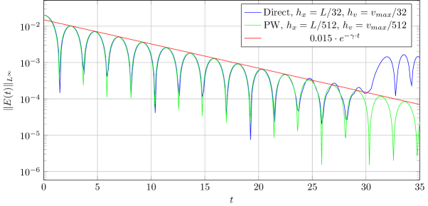
Figure 1: Electric field amplitude for the weak Landau damping benchmark. The direct method (blue graph) uses $h_{x}=\frac{L}{32}$, $h_{v}=\frac{v_{\max}}{32}$, $\Delta t=\frac{1}{8}$, fourth order classical Runge–Kutta method and kernels of order $n=2$. The PW method (green graph) uses $h_{x}=\frac{L}{512}$, $h_{v}=\frac{v_{\max}}{512}$, $\Delta t=\frac{1}{16}$, symplectic Euler method and also kernels of order $n=2$. Up to $t=25$ the numerical damping rate of both methods are in good agreement with the theoretical prediction. At $t\approx 29$ the recurrence effect sets in for the direct method, and between $t=24$ and $29$ the amplitude maxima are slightly overshooting their theoretical value. The PW method, on the other hand, reproduces the correct damping behaviour until $t=35$.

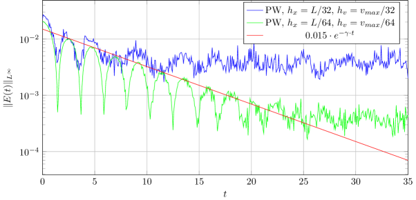
Figure 2: Amplitude of $E_{h,\sigma}$ when running PW method with low resolution, resolution and parameters as for the direct method above.

Figure 1 shows the evolution of the electric field amplitude over time. From theory and numerical experiments we know that the electric field will get damped periodically at rate $\gamma=0.153359$ and oscillation frequency $\omega=1.41566$[41]. Until $t\approx 25$ both methods are in good agreement with theory. At this point we observe a recurrence phenomenon for the direct approach: the electric field amplitude increases again and a new damping process begins. This is remarkable as recurrence has been known for grid-based solvers[42], but is has been claimed that particle methods do not suffer from this effect[43]. Conventional blob methods, however, become ‘noisy’ at this stage, and we believe that it is this noise that masks the recurrence[23, 5, 2].

The cause of this phenomenon can be seen in Figure 3, which shows the evolution of the difference between the numerical solution $f_{h,\sigma}$ and the Maxwellian distribution $f_{M}$. One can observe waves of increasing frequency entering the domain from $v\rightarrow\pm\infty$. Starting at $t=30$, unphysical artefacts appear in the plot of the direct method. At this point we can observe an aliasing effect: the high-frequency modes are not correctly captured by the low resolution of the direct method. The higher resolution of the PW method, however, can correctly reproduce $f$ for extended period of times.

In the limit $t\rightarrow+\infty$ and for the initial datum (30) the analytic solution $f(t,\cdot,\cdot)$ will weakly converge to a steady state but not in a strong sense[14]. The solution $f$ develops waves of increasing frequency and number with time and therefore develops a small scale structure. Thus the PW method will eventually suffer from recurrence as well.

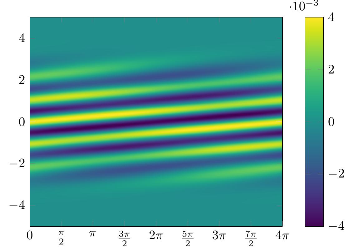
(a) Direct, $t=10$

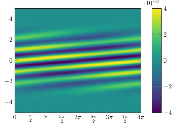
(b) PW, $t=10$

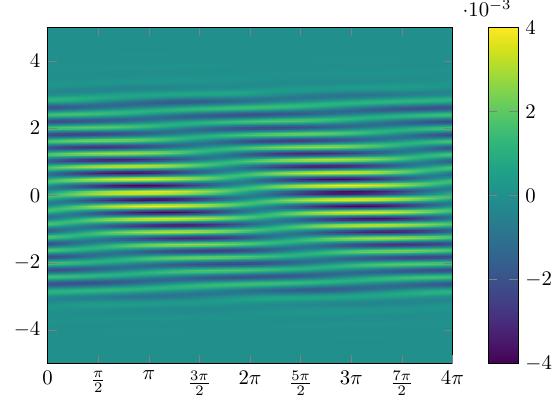
(c) Direct, $t=30$

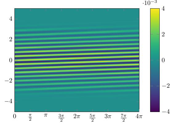
(d) PW, $t=30$

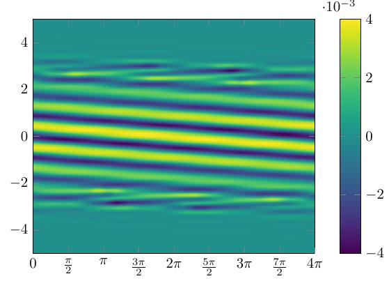
(e) Direct, $t=50$

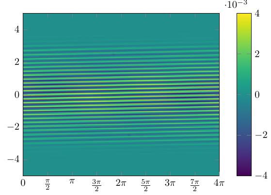
(f) PW, $t=50$

Figure 3: Difference between the numerical solution $f_{h,\sigma}$ and the Maxwellian equilibrium $f_{M}$ for the weak Landau damping benchmark. On the left-hand-side $f_{h,\sigma}$ is computed via the direct method and on the right-hand-side using the PW method. The resolutions are the same as in Figure 1. For $t\leq 30$ the number of waves is steadily increasing. For the lower resolution, starting at $t=30$, numerical artefacts can be observed. At $t=50$ aliasing occurs: the spatial resolution is insufficient to capture the highest frequencies. Therefore high frequencies appear as low ones. The high-resolution solution can resolve the solution correctly up to $t=50$.

In Figure 4 we display the results of running the PW method at low resolution; nameley the same number of particles and the same scaling parameters as for the direct method. Along the boundaries of the boxes $B$ one observes errors caused by the discontinuity of the PW approximations. This also leads to noisy results in the amplitude plot, Figure 2. Note however, that for a discontinuous function the $L^{\infty}$-norm is not suitable to analyse errors and therefore the noisy results in below figure are to be expected when using to low resolutions. Still even though there are strong errors along the boundaries of the cover boxes, the overall dynamic in $f$ is correctly captured to a similar extend as for the direct method. Especially one observes a similar wave-structure for $t=10,30$ and $50$ when comparing Figures 3(a) and 3(e) with Figures 4(b) and 4(d).

This leads to the conclusion that using the PW method starts to be reasonable when discontinuity errors are on the same level as the local interpolation errors, which can only be expected for high enough resolutions. When looking at Figure 2 we see that doubling the resolution from $h_{x}=L/32$ and $h_{v}=v_{\mathrm{max}}/32$ to $h_{x}=L/64$ and $h_{v}=v_{\mathrm{max}}/64$ already significantly lowers the errors in the amplitude plots, suggesting that the latter resolution is the lowest resolution to get reasonable results with PW methods for this set of parameters and this benchmark. This also the reason why we chose to run our tests for the PW method with $h_{x}=L/512$ and $h_{v}=v_{\mathrm{max}}/512$, i. e., a relatively high resolution. Note that the direct method can be run with lower resolution and still produce good results, however, takes significantly longer to run and uses significantly more resources. This is why we decided to run the test for the direct method in the relatively low resolution only. The performance and accuracy trade-off between the direct and PW method will be discussed in more detail later in Section 6.4 and Section 6.5.

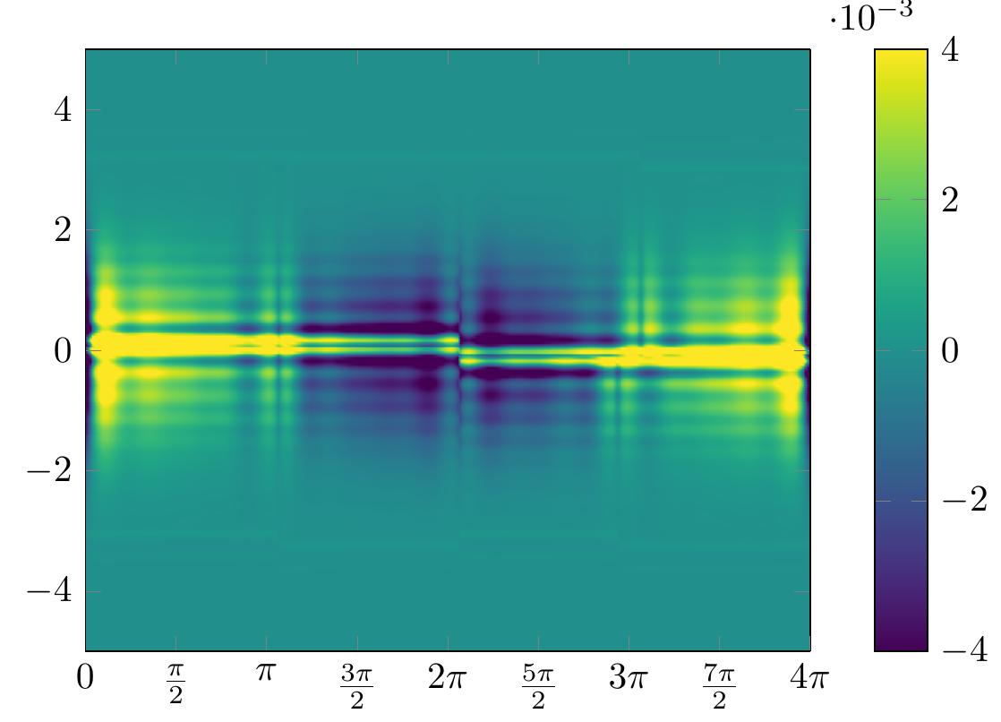
(a) $t=0$

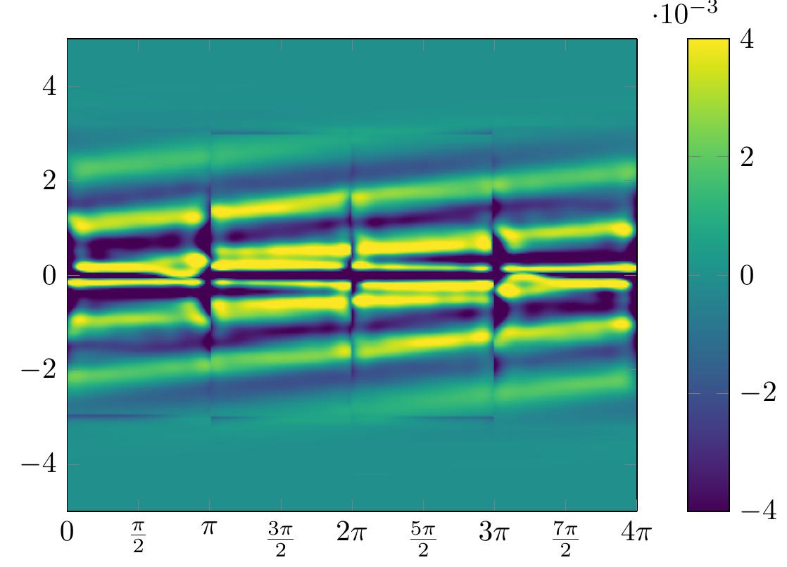
(b) $t=10$

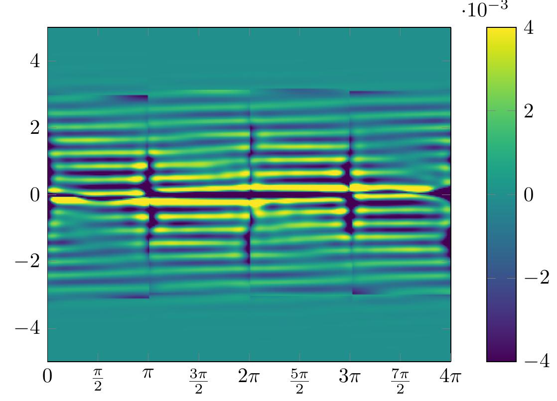
(c) $t=30$

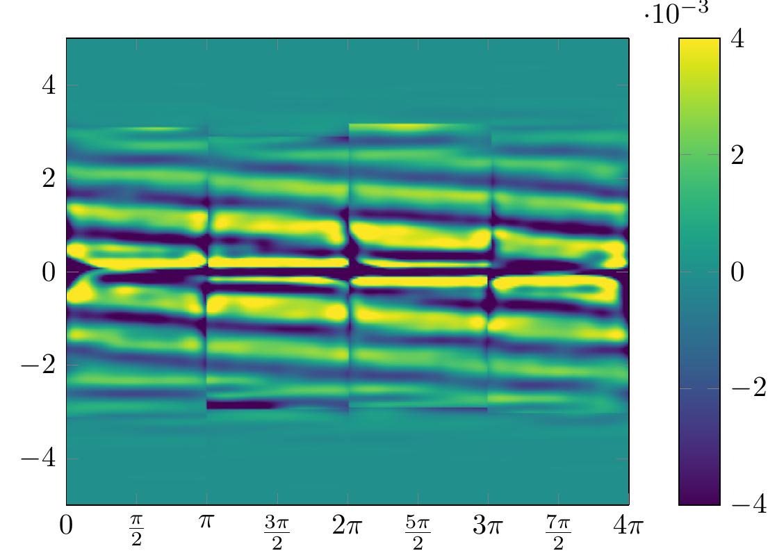
(d) $t=50$

Figure 4: Difference between $f_{h,\sigma}$ and $f_{M}$ for the weak Landau damping benchmark when using the PW method at a low resolution, equal to that of the direct method. One observes jumps in the errors along the boundaries of the boxes $B$ used in the sub-division of the phase space. However, the simulation still captures the correct global dynamic of $f$.

In figure 5 we compare the domain decomposition using the $kd$-tree for different times in the simulation using $h_{x}=\frac{L}{512}$ and $h_{x}=\frac{v_{\mathrm{max}}}{512}$. We notice that the decomposition essentially stays close to an uniform grid for both $t=0$ and $t=50$. The strongest adaptation can be observed where waves enter the domain, around $|v|\approx 3$.

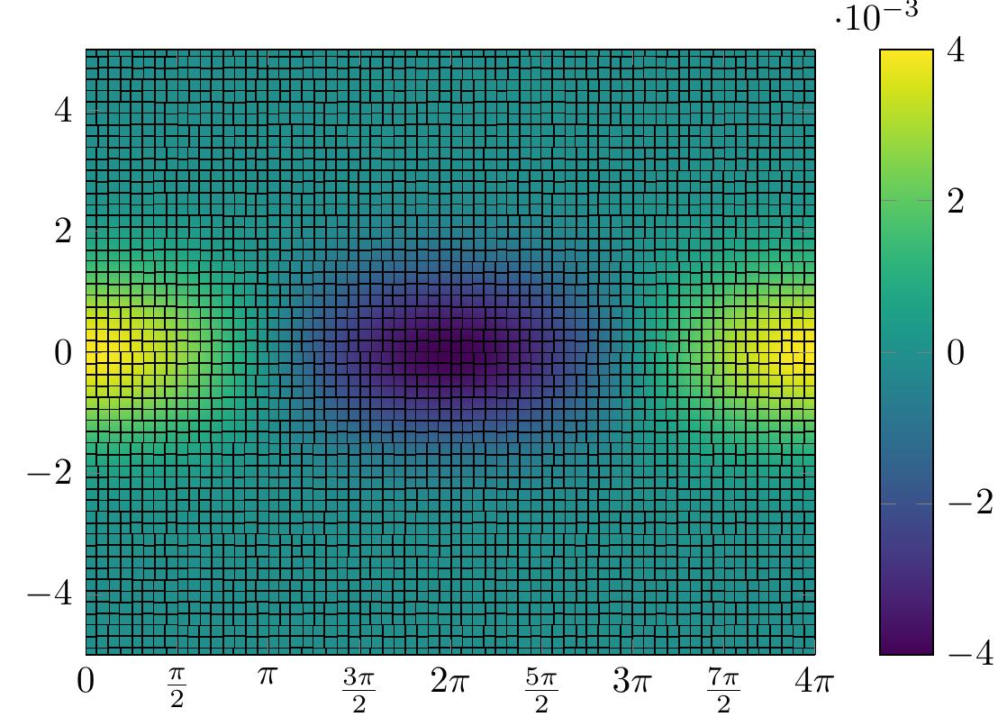
Figure 5: Comparison between domain decompositions for the PW method for $t=0$ and $t=50$ for the weak Landau damping benchmark using $h_{x}=\frac{L}{512}$ and $h_{x}=\frac{v_{\mathrm{max}}}{512}$.

6.2 Two stream instability

For our second benchmark we consider the initial condition

$$f_{0}(x,v)=\frac{1}{\sqrt{2\pi}}v^{2}e^{-\frac{v^{2}}{2}}\big{(}1+\alpha\cos(kx)\big{)},\quad(x,v)\in[0,L]\times\mathbb{R}$$ (31)

with $\alpha=0.01$, $k=0.5$, $L=4\pi$. We use $v_{\max}=8$ as cut-off in velocity-space. The two stream instability simulates two particle streams of same density but opposing velocities colliding with each other. The initial state is a slight perturbation of the instable equilibrium

$$f_{eq}(v)=\frac{1}{\sqrt{2\pi}}v^{2}e^{-\frac{v^{2}}{2}}.$$

We used $h_{x}=\frac{L}{64}$ and $h_{v}=\frac{v_{\max}}{128}$ for the direct method and $h_{x}=\frac{L}{512}$ and $h_{v}=\frac{v_{\max}}{1024}$ for the PW method. The scaling parameters were fixed as $\sigma_{x}=2$, $\sigma_{v}=1$ for the direct method and $\sigma_{x}=4$, $\sigma_{v}=2$ for the PW method. For both methods we used fourth order kernels. The time-steps are set to $\Delta t=\frac{1}{4}$ and $\Delta t=\frac{1}{32}$ with classical Runge-Kutta and symplectic Euler as time-integrators respectively.

The evolution of the electric field’s amplitude is depicted in Figure 6. Because the direct approach is limited to fairly small numbers of particles, i. e., coarse resolutions, it performs worse than the PW method. However, the direct method is still able to capture the dynamics of both $f$ and $E$ qualitatively correctly. The forming of the filaments introduces steep gradients. This results in overshoots in the numerical solution, as soon as these gradients can no longer be resolved by the fixed resolution.

This can cleary be observed in Figure 7 after $t\approx 30$ in the plots for the direct method. While the direct and PW methods, similar to grid-based methods, suffer from overshoots and thus do not provide good accuracy for extended times in turbulent simulations, they reproduce the fine details of $f$ better than Eulerian or PIC methods.

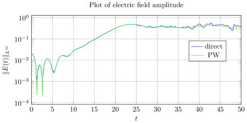
Figure 6: Electric field amplitude for the two stream instability. The direct method (blue) used $h_{x}=\frac{L}{64}$, $h_{v}=\frac{10}{128}$, $\Delta t=\frac{1}{4}$ and the classical Runge-Kutta method. The PW method (green) used $h_{x}=\frac{L}{512}$, $\frac{10}{1024}$, $\Delta t=\frac{1}{32}$ and the symplectic Euler method. Both the direct and PW method employed fourth order kernels. After an initial damping until $t\approx 5$ the mixing process starts dominating the dynamics. The electric field amplitude arrives at its maximum at approximately $t\approx 23$ and starts periodically oscillating afterwards. Until $t\approx 23$ the increase of amplitude is captured correctly by both methods. After $t\approx 25$ slight numerical artefacts appear in the solution computed with lower resolution.

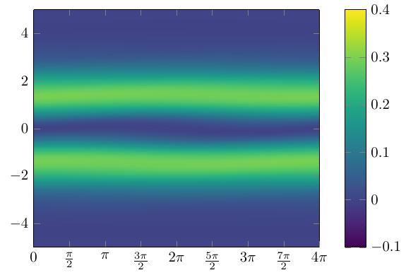
(a) Direct, $t=10$

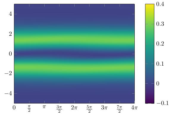
(b) PW, $t=10$

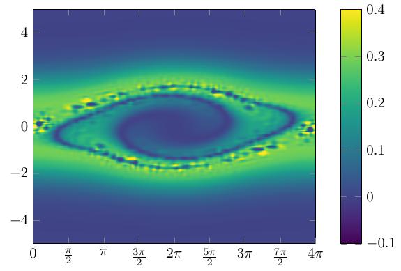
(c) Direct, $t=30$

(d) PW, $t=30$

(e) Direct, $t=50$

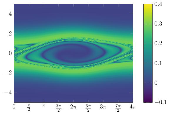
(f) PW, $t=50$

Figure 7: The distribution function $f_{h,\sigma}(t,x,v)$ for the two stream instability benchmark. The numerical solution computed using the direct method is on the left-hand side, the PW method on the right-hand side. The parameters were chosen as in Figure 6. At $t\approx 10$ the phase-space ‘vortex’ starts to form. After $t=30$ one can observe the ‘vortex’ rotation. With each rotation further filaments enter the ‘vortex’. It can also be observed that the filaments enter at $x=0$ or $x=4\pi$ and drift towards the center of the ‘vortex’. While both methods reproduce the dynamics of $f$ qualitatively correct, the errors made by the direct method are significantly higher. Both methods suffer from overshoots near filaments.

In Figure 8 we compare the domain decompositions of the PW scheme for different times $t$ using $h_{x}=\frac{L}{512}$ and $h_{x}=\frac{v_{\mathrm{max}}}{1024}$. At $t=0$ it is close to a uniform grid. This is expected due to the uniforml particle distribution at $t=0$. Later, at $t=50$ the particles are in more disarray and thus we observe some adaptation of the domain decomposition. However, the decompositions seem to be still close to an uniform grid, suggesting that the particle distribution is also still quasi-uniform. The strongest adaptations can be seen close to the filaments.

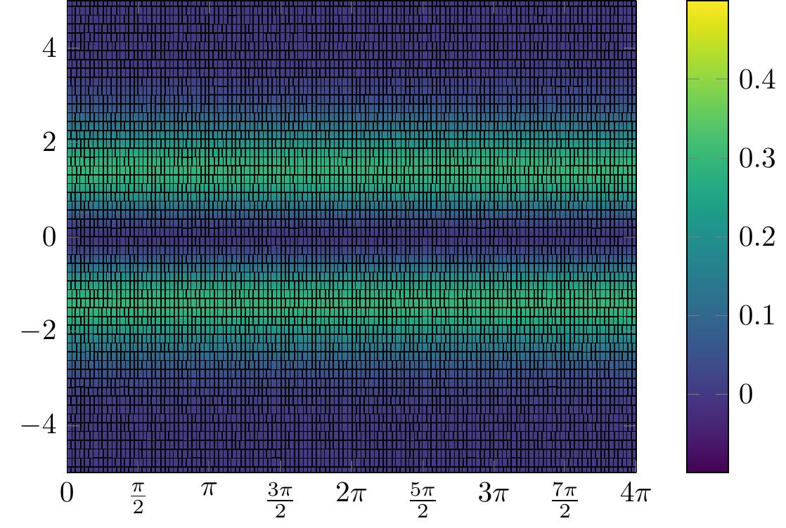
Figure 8: Comparison between domain decompositions for the PW method for $t=0$ and $t=50$ for the two stream benchmark using $h_{x}=\frac{L}{512}$ and $h_{x}=\frac{v_{\mathrm{max}}}{1024}$.

6.3 Bump on tail instability

The initial condition for our final benchmark, the bump on tail instability, is

$$f_{0}(x,v)=\frac{1}{\sqrt{2\pi}}\left(n_{p}\cdot e^{-\frac{v^{2}}{2}}+n_{b}\cdot e^{-\frac{1}{2}\frac{(v-v_{b})^{2}}{v_{t}^{2}}}\right)\left(1+\alpha\cos(kx)\right).$$ (32)

with $n_{p}=0.9$, $n_{b}=0.2$, $v_{b}=4.5$, $v_{t}=0.5$, $\alpha=0.04$, $k=0.3$, $L=\frac{2\pi}{0.3}$[41]. The cut-off in velocity space is set to $v_{\max}=10$. For this test case we only consider the PW method and are interested in both long- and short-term accuracy. We chose $h_{x}=\frac{L}{1024}$ and $h_{v}=\frac{v_{\max}}{512}$ as resolution and second order kernels. The scaling parameters were set to $\sigma_{x}=6$, $\sigma_{v}=3$. The time-step is set to $\Delta t=\frac{1}{16}$ and the symplectic Euler time integration method was used.

The bump on tail instability simulates the clash of a low density particle stream with Maxwellian velocity distribution around $v_{b}=4.5$ into resting particles, i. e., with Maxwellian velocity distribution around $0$. The equilibrium state

$$f_{eq}(v)=\frac{1}{\sqrt{2\pi}}\left(n_{p}\cdot e^{-\frac{v^{2}}{2}}+n_{b}\cdot e^{-\frac{1}{2}\frac{(v-v_{b})^{2}}{v_{t}^{2}}}\right)$$

gets slightly perturbed, whereby the mixing process is initiated. The resulting dynamics can be described as an overlapping of the effects of weak Landau damping and the two stream instability, i. e., an overlapping of mixing and damping processes. Which effect dominates, depends on the difference in density and the strength of the initial perturbation.

For the chosen set of parameters, the damping effect on electric field is small and only becomes apparent at large time intervals. Therefore the benchmark involves being able to simulate the correct behaviour for times $t\gg 100$. In Figure 10 one sees the long time damping, which is in good agreement with the results presented by Arber and Vann[41].

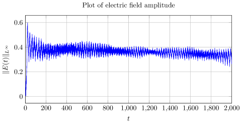
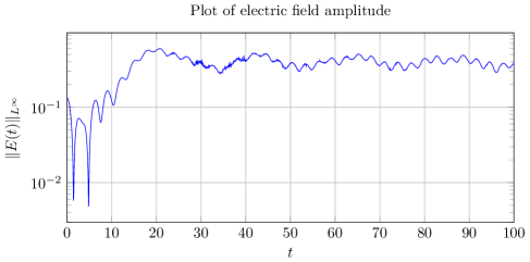
Figure 9: Amplitude of the electric field until $T=2000$ for the bump on tail instability benchmark. The simulation was run at resolution $h_{x}=\frac{L}{1024}$, $h_{v}=\frac{10}{512}$ and time step $\Delta t=\frac{1}{16}$ using the symplectic Euler method. After an initial increase of amplitude, several oscillation modes can be observed. In the long time limit $t\rightarrow 2000$ the amplitude gets gradually damped.

Figure 10: Amplitude of the electric field of the bump on tail instability until $T=50$ with simulation parameters as in figure Figure 10. After an initial damping until $t\approx 5$ the amplitude increases to reach its global maximum at $t\approx 20$. Then there are two dominating oscillation modes, a slow oscillation with period $\approx 22$ and another faster oscillation with period $\approx 2.5$. The first oscillation is caused by the mixing of the two particle streams, see Figure 6, the second oscillation is caused by a Landau damping effect, see Figure 1. Between $t=30$ and $t=40$ one can observe numerical noise. At this point the mixing of the two streams is causing steep gradients and thus overshoots in the numerical solution $f_{h,\sigma}$ which results in numerical errors when computing $E_{h,\sigma}$. After $t=50$, the amplitude is reproduced correctly again.

In Figure 10 we see an initial damping between $t=0$ and $t\approx 5$. On the one hand, after $t\approx 5$ a ‘vortex’ begins to form that will eventually dominate the dynamics for early times. The ‘vortex’ moves periodically in phase space along the $x$-axis. This can be seen in Figure 11. After $t\approx 20$ an increase in the number of filaments can be observed. This effect is similar to that of Figure 7 from the two stream instability simulation.

On the other hand, starting at $t\approx 20$ one can observe waves forming on the particle cluster centred at $v=0$. This is comparable to weak linear Landau damping, see Figure 3. Note, that compared to the previous two benchmarks, the perturbation strength $\alpha=0.04$ is significantly higher and thus the amplitudes of appearing waves are higher as well.

Similar to the two stream instability benchmark, we observe overshoots resulting in slight numerical noise in this simulation, see Figures 11(e) and 11(f). But in contrast to the two stream instability benchmark, the gradients do not get as steep and therefore the simulation stays stable even with fewer particles and for extended periods of time.

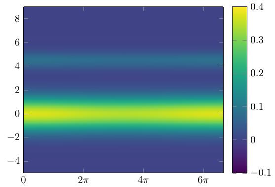
(a) $t=0$

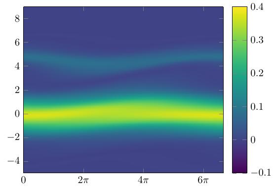
(b) $t=10$

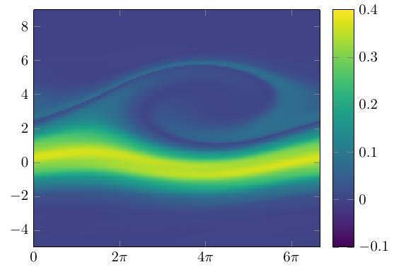
(c) $t=20$

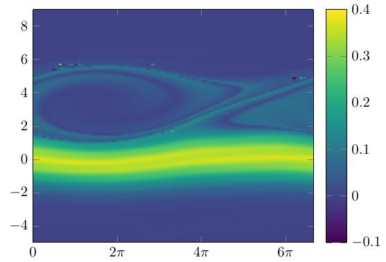
(d) $t=30$

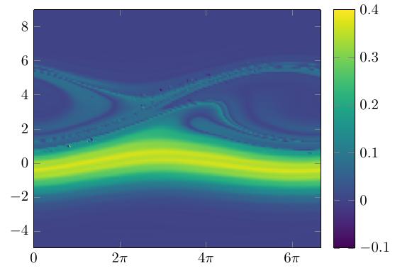
(e) $t=40$

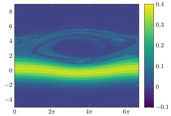
(f) $t=50$

Figure 11: Evolution of the distribution function $f_{h,\sigma}(t,x,v)$ until $T=50$ for the bump on tail instability. Computed using the PW method with the same parameters as in Figure 10. Beginning at $t\approx 10$ the phase-space ‘vortex’ starts to form and gets fully developed at $t\approx 20$. Afterwards it starts periodically moving along the x-axis with a period of $\approx 22$ which coincides with the slow oscillation in Figure 10. After $t=20$ the formation of so-called Langmuir waves on the bigger particle cluster can be observed. This coincides with the faster oscillations appearing in Figure 10 with period $\approx 2.5$.

6.4 Convergence study

In this section we investigate the convergence behaviour of the presented methods in the setting of the weak Landau damping benchmark, see Section 6.1. In particular we compare both the performance and accuracy of the direct and PW methods. We compute the errors for $f_{h,\sigma}$ with respect to a reference solution with $h_{x}=\tfrac{L}{4096}$, $h_{v}=\tfrac{v_{\mathrm{max}}}{4096}$ using the PW method and second order kernels. Note that we use the PW method for the reference solution as computation of a global interpolant in this resolution is not feasible from both memory usage and run-time perspective on the machine we used.

For all benchmarks we used the classical Runge–Kutta method with $\Delta t=\frac{1}{8}$ for the direct approach and the symplectic Euler time-integration scheme with $\Delta t=\frac{1}{16}$ for the PW approach. The minimal box-size for the PW method was set to $N_{\mathrm{min}}=100$.

The $L^{2}$- and $L^{\infty}$-errors for both schemes when using kernels of order $n=2$ are displayed in Figures 12 and 13. The corresponding results for kernels of order $n=4$ are given in Figures 14 and 15.

For all of these approaches, the error does not significantly grow with time $t$; no ‘noise’ becomes visibible. For the direct method the $L^{2}$ and $L^{\infty}$-errors are of similar magnitude. Surprisingly, this is also the case for the $PW$ method, albeit to a somewhat lesser extent. This lesser extent can be attributed to the fact that the discontinuities of the PW approach more strongly affect the $L^{\infty}$-norm than the $L^{2}$-norm.

For the direct method we observe a rapid decrase of the error with increasing resoltion. We empirically observe convergence rates of $\mathcal{O}(h^{5.5})$ and $\mathcal{O}(h^{7})$ in the $L^{2}$-norm for respectively $n=2$ and $n=4$, clearly exceeding the expected rates.

For the PW approach, convergence only starts later, at higher resolutions and does not reach the same rates as the direct method does. Here empirical convergence rates approach $\mathcal{O}(h^{3})$ and $\mathcal{O}(h^{4.5})$ in the $L^{2}$-norm respectively for orders $n=2$ and $n=4$; much closer to the expected rates.

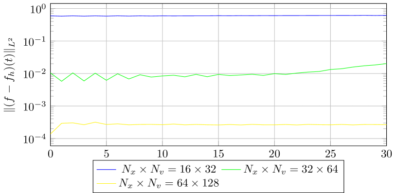
(a) Direct

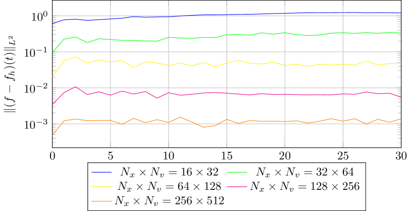
(b) PW

Figure 12: A comparison of $L^{2}$-errors for $f_{h,\sigma}$ in time using second order kernels and $\sigma_{x}=1$ and $\sigma_{v}=0.5$. Left the direct and on the right the PW approach was used. One observes a higher convergence order for the direct approach exceeding the theoretically predicted convergence order of $O(h^{3})$, while the observed convergence order for the PW method is slightly below the predicted convergence order.

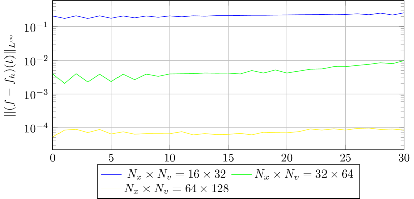
(a) Direct

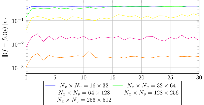
(b) PW

Figure 13: A comparison of $L^{\infty}$-errors for $f_{h,\sigma}$ in time using second order kernels and $\sigma_{x}=1$ and $\sigma_{v}=0.5$. Left the direct and on the right the PW approach was used. One observes a higher convergence order for the direct approach, however, both approaches exceed the theoretically predicted convergence order of $O(h^{2.5})$.

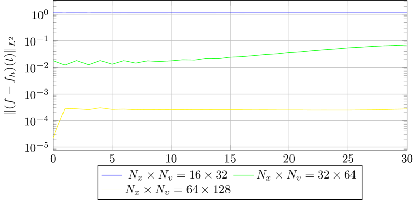
(a) Direct

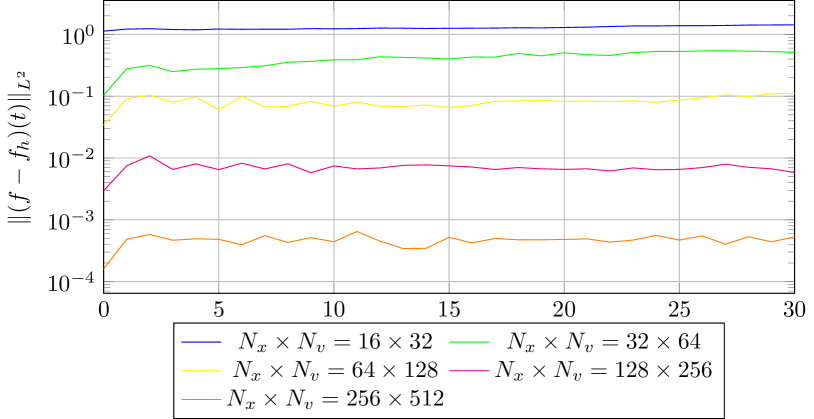
(b) PW

Figure 14: A comparison of $L^{2}$-errors for $f_{h,\sigma}$ in time using fourth order kernels and $\sigma_{x}=1$ and $\sigma_{v}=0.5$. Left the direct and on the right the PW approach was used. One observes a higher convergence order for the direct approach again exceeding the theoretically predicted convergence order of $O(h^{5})$. For the PW method one observes a slighlty lower convergence order than expected.

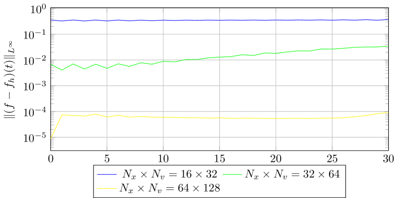
(a) Direct

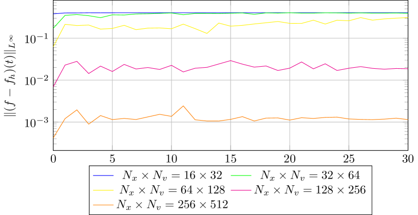
(b) PW

Figure 15: A comparison of $L^{\infty}$-errors for $f_{h,\sigma}$ in time using fourth order kernels and $\sigma_{x}=1$ and $\sigma_{v}=0.5$. Left the direct and on the right the PW approach was used. One observes a higher convergence order for the direct approach exceeding the theoretically predicted convergence order of $O(h^{4.5})$. For the PW method one observes a slighlty lower convergence order than expected.

6.5 Computational Efficiency

In Tables 2, 3, 4 and 5 we give the timings for a single time-step in the weak Landau damping test-case. The hardware hardware has the following specfications:

CPU	Intel(R) Xeon(R) E-2276M CPU @ 2.80GHz
	6 cores
RAM	32 GB DDR4 Synchronous 2667 MHz

For the direct approach only resulutions up to $h_{x}=L/64$, $h_{v}=v_{\mathrm{max}}/64$ were tested, due to memory constraints. When comparing the timings for a single time-step for the direct and PW methods, we observe that the PW method is always significantly faster. Even for low resolutions the PW method is still at least one order of magnitude faster than the direct method. Thus we conclude that from a performance perspective the PW method is indeed always the best choice. In particular, Tables 4 and 5 confirm that the PW method scales linearly in the number of particles.

Figures 12 and 15 show that for a given resolution, the direct method is up to two orders of magnitude more accurate than the PW method. However, this comparison is misleading: the PW requires higher resolutions to reach the same accuracy, but still needs significantly less computational time to do so.

Resolution	$t_{step}$ in s	$t_{total}$ in s
$h_{x}=L/16$, $h_{v}=v_{\mathrm{max}}/16$	$2.03\cdot 10^{-2}$	4.92
$h_{x}=L/32$, $h_{v}=v_{\mathrm{max}}/32$	$1.78\cdot 10^{-1}$	43.0
$h_{x}=L/64$, $h_{v}=v_{\mathrm{max}}/64$	5.62	1360

Table 2: Timings for the direct approach using second order kernels.

Resolution	$t_{step}$ in s	$t_{total}$ in s
$h_{x}=L/16$, $h_{v}=v_{\mathrm{max}}/16$	$2.43\cdot 10^{-2}$	5.89
$h_{x}=L/32$, $h_{v}=v_{\mathrm{max}}/32$	$2.54\cdot 10^{-1}$	61.5
$h_{x}=L/64$, $h_{v}=v_{\mathrm{max}}/64$	7.16	1730

Table 3: Timings for the direct approach using fourth order kernels.

Resolution	$t_{step}$ in s	$t_{total}$ in s
$h_{x}=L/16$, $h_{v}=v_{\mathrm{max}}/16$	$1.22\cdot 10^{-3}$	0.590
$h_{x}=L/32$, $h_{v}=v_{\mathrm{max}}/32$	$2.77\cdot 10^{-3}$	1.34
$h_{x}=L/64$, $h_{v}=v_{\mathrm{max}}/64$	$9.05\cdot 10^{-3}$	4.28
$h_{x}=L/128$, $h_{v}=v_{\mathrm{max}}/256$	$3.00\cdot 10^{-2}$	14.3
$h_{x}=L/256$, $h_{v}=v_{\mathrm{max}}/512$	$1.15\cdot 10^{-1}$	55.7

Table 4: Timings for the PW approach using second order kernels.

Resolution	$t_{step}$ in s	$t_{total}$ in s
$h_{x}=L/16$, $h_{v}=v_{\mathrm{max}}/16$	$2.29\cdot 10^{-3}$	1.11
$h_{x}=L/32$, $h_{v}=v_{\mathrm{max}}/32$	$5.94\cdot 10^{-3}$	2.88
$h_{x}=L/64$, $h_{v}=v_{\mathrm{max}}/64$	$1.90\cdot 10^{-2}$	9.18
$h_{x}=L/128$, $h_{v}=v_{\mathrm{max}}/256$	$6.45\cdot 10^{-2}$	31.2
$h_{x}=L/256$, $h_{v}=v_{\mathrm{max}}/512$	$2.55\cdot 10^{-1}$	123

Table 5: Timings for the PW approach using fourth order kernels.

Resolution	$t_{step}$ in s	$t_{total}$ in s
$h_{x}=L/16$, $h_{v}=v_{\mathrm{max}}/16$	$1.07\cdot 10^{-4}$	$2.57\cdot 10^{-2}$
$h_{x}=L/32$, $h_{v}=v_{\mathrm{max}}/32$	$1.63\cdot 10^{-4}$	$3.92\cdot 10^{-2}$
$h_{x}=L/64$, $h_{v}=v_{\mathrm{max}}/64$	$2.90\cdot 10^{-4}$	$6.94\cdot 10^{-2}$
$h_{x}=L/128$, $h_{v}=v_{\mathrm{max}}/256$	$9.37\cdot 10^{-4}$	$2.25\cdot 10^{-1}$
$h_{x}=L/256$, $h_{v}=v_{\mathrm{max}}/512$	$4.40\cdot 10^{-3}$	1.06

Table 6: Timings for a simple PIC method.

Finally we also compare the PW method with a simple PIC method. Our PIC code approximates the density $\rho(x)$ for $jh_{x}\leq x<(j+1)h_{x}$ by adding the masses of all particles in that $x$-range, and dividing the result by $h_{x}$. The electric potential $\varphi$ is approximated using a standard second-order finite-element method, time-integration uses the classical Runge–Kutta scheme with time-step $\Delta t=\frac{1}{8}$. Figures 16 and 17 show the resulting errors in the elictric field.

One observes that the PW method converges significantly faster in both the $L^{2}$ and $L^{\infty}$-norm. This is in particular the case for the finest resolutions. On the other hand, the simple PIC code is significantly faster for a given resolution, as can be seen by comparing Tables 5 and 6. However, the high $L^{\infty}$-errors for the PIC method suggest a strong level of numerical noise, which is much less present in the PW method. Here, especially in the $L^{2}$-sense, it is much less clear at which level of accuracy the PW method will begin to outperform the PIC method. On the other hand, it is clear that the PIC method will require significantly larger numbers of particles and thus imposes larger memory constraints on the machine.

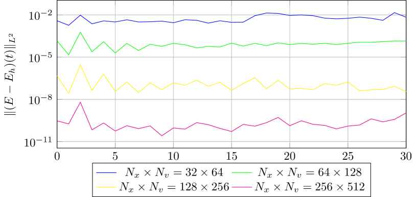
(a) PW, 4.order

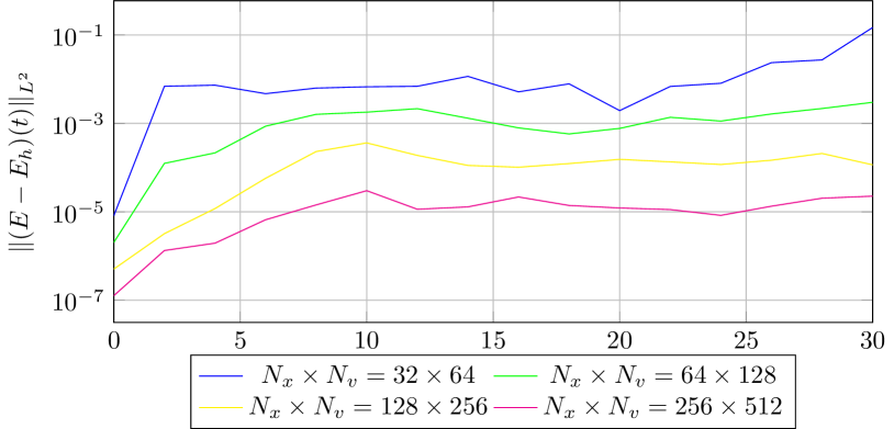
(b) PIC

Figure 16: A comparison of $L^{2}$-errors for the numerically computed electric field using on the one hand the PW method with fourth order kernels and $\sigma_{x}=1$, $\sigma_{v}=0.5$, and, on the other hand, a simple PIC method.

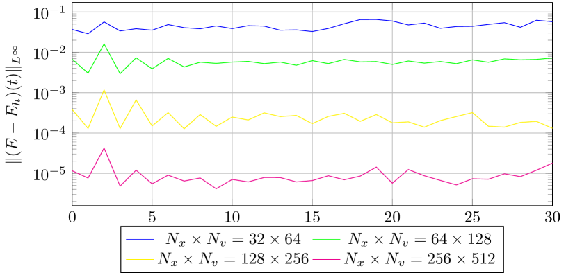
(a) PW, 4.order

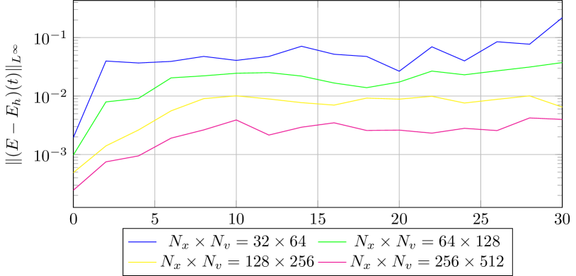
(b) PIC

Figure 17: A comparison of $L^{\infty}$-errors for the numerically computed electric field using on the one hand the PW method with fourth order kernels and $\sigma_{x}=1$, $\sigma_{v}=0.5$, and, on the other hand, a simple PIC method.

7 Conclusion

We have presented a particle method using meshfree interpolation of arbitrary high order and investigated numerically, whether the good convergence behaviour from RKHS theory carries over to the case of the fully non-linear Vlasov-Poisson equation in the $d=1$ case.

In contrast to conventional particle methods like PIC or SPH, our method does not need a remapping strategy to avoid numerical noise. Furthermore, as interpolation with Wendland kernels is stable with arbitrary high convergence order, our method needs significantly fewer particles to achieve the same accuracy as classical particle methods. The downside is that our method struggles with steep gradients, which naturally appear in solutions of the Vlasov–Poisson equation. To resolve them correctly, any interpolation method needs high resolution, irrespective of the convergence order of the method. Similar problems can be observed with higher order Eulerian Vlasov solvers. Steep gradients lead to overshoots. However, while negative values of $f$ do not make any physical sense, their effect on the quantities $\rho$ and $E$ seems to be limited.

The ill-conditioning of the kernel matrices is a well-known problem and its solution is an ongoing research topic in the RKHS community. This limits the particle numbers for the direct method. In case of the Vlasov–Poisson equation, however, this problem can to some extend be bypassed by using piece-wise interpolants instead. Our simulations have illustrated that this approach does in fact result in efficient Lagrangian schemes, albeit with convergence orders that are lower than those of the direct approach.

To summarise, at least in the one-dimensional case, the presented PW method offers a good compromise between the stability and high accuracy of purely Eulerian methods on the one hand and speed and hyperbolicity of classical particle methods on the other hand, while avoiding the inherent numerical noise of the latter.

It is unclear whether the piecewise approach is suitable for higher dimensions, for which we expect reduced efficiency as larger local systems need to be solved. On the other hand, we believe that the piece-wise approach could prove to be beneficial for stellar dynamics, where particles tend cluster more stronlgy, and could thus provide ‘auto-adaptation’. These points require further investigation.

References

- [1] P.A. Raviart “An analysis of particle methods” In Numerical Methods in Fluid Dynamics, 1985, pp. 243–324 DOI: 10.1007/BFb0074532
- [2] Jakob Ameres “Stochastic and Spectral Particle Methods for Plasma Physics”, 2018
- [3] F. Filbet and E. Sonnendrücker “Comparison of Eulerian Vlasov Solvers” In Computer Physics Communications 150.3, 2001, pp. 247–266 DOI: 10.1016/S0010-4655(02)00694-X
- [4] F. Filbet, E. Sonnendrücker and P. Bertrand “Conservative Numerical Schemes for the Vlasov Equation” In Journal of Computational Physics 172.1, 2001, pp. 166–187 DOI: 10.1006/jcph.2001.6818
- [5] B. Wang, G. H. Miller and P. Colella “A Particle-in-cell Method with Adaptive Phase-space Remapping for Kinetic Plasmas” In SIAM J. Sci. Comput. 33.6, 2011, pp. 3509–3537 DOI: 10.1137/100811805
- [6] Matthias Kirchhart and Christian Rieger “Discrete Projections: A Step Towards Particle Methods on Bounded Domains without Remeshing” In SIAM Journal on Scientific Computing 43.1, 2021, pp. A609–A635 DOI: 10.1137/19M1299864
- [7] A.A. Vlasov “On the vibrational properties of an electronic gas” In Zh. Eksp. Teor. Fi. 8, 291, 1938
- [8] L.D. Landau “On the Vibrations of the Electronic Plasma” In Collected Papers of L.D. Landau Pergamon, 1965, pp. 445–460 DOI: 10.1016/B978-0-08-010586-4.50066-3
- [9] A.A. Arsen’ev “Global existence of a weak solution of Vlasov’s system of equations” In USSR Computational Mathematics and Mathematical Physics 15.1, 1975, pp. 131–143 DOI: 10.1016/0041-5553(75)90141-X
- [10] A.A. Arsenev “Existence and uniqueness of the classical solution of Vlasov’s system of equations” In Zhurnal Vychislitelnoi Matematiki i Matematicheskoi Fiziki 15, 1975, pp. 1344–1349
- [11] S. Ukai and T. Okabe “On classical solutions in the large in time of two-dimensional Vlasov’s equation” In Osaka Journal of Mathematics 15.2, 1978, pp. 245–261
- [12] K. Pfaffelmoser “Global classical solutions of the Vlasov–Poisson system in three dimensions for general initial data” In Journal of Differential Equations 95.2, 1992, pp. 281–303 DOI: 10.1016/0022-0396(92)90033-J
- [13] P.L. Lions and B. Perthame “Propagation of moments and regularity for the 3-dimensional Vlasov–Poisson system” In Inventiones mathematicae 105.1, 1991, pp. 415–430 DOI: 10.1007/BF01232273
- [14] C. Mouhot and C. Villani “On Landau damping” In Acta Mathematica 207.1, 2011, pp. 29–201 DOI: 10.1007/s11511-011-0068-9
- [15] C.K. Birdsall and A.B. Langdon “Plasma Physics via Computer Simulation”, Series in Plasma Physics Taylor & Francis, 2004
- [16] R.T. Glassey “The Cauchy Problem in Kinetic Theory” Society for IndustrialApplied Mathematics, 1996 DOI: 10.1137/1.9781611971477
- [17] L. Rosenhead “The Formation of Vortices from a Surface of Discontinuity” In Proceedings of the Royal Society of London 142.832, 1931, pp. 170–192
- [18] F.H. Harlow “Hydrodynamic Problems involving large Fluid distortions” In Journal of the Association of computing machinery 4, 1954, pp. 137–142 DOI: 10.1145/320868.320871
- [19] M.W. Evans and F.H. Harlow “The Particle-In-Cell method for Hydrodynamic Calculations” In Report LA-2139, Los Alamos Scientific laboratory of the university of California, 1957
- [20] G.-H. Cottet and P.-A. Raviart “Particle Methods for the One-Dimensional Vlasov–Poisson Equations” In SIAM Journal on Numerical Analysis 21.1, 1984, pp. 52–76 DOI: 10.1137/0721003
- [21] R.W. Hockney and J.W. Eastwood “Computer Simulation Using Particles” CRC Press, 2021
- [22] J Denavit “Numerical simulation of plasmas with periodic smoothing in phase space” In Journal of Computational Physics 9.1, 1972, pp. 75–98 DOI: 10.1016/0021-9991(72)90037-X
- [23] A. Myers, P. Colella and B. Straalen “A 4th-Order Particle-in-Cell Method with Phase-Space Remapping for the Vlasov–Poisson Equation” In SIAM Journal on Scientific Computing 39.9, 2016, pp. B467–B485 DOI: 10.1137/16M105962X
- [24] G. H. Cottet and P. A. Raviart “On particle-in-cell methods for the Vlasov-Poisson equations” In Transport Theory and Statistical Physics 15.1-2 Taylor & Francis, 1986, pp. 1–31 DOI: 10.1080/00411458608210442
- [25] N. Besse and E. Sonnendrücker “Semi-Lagrangian schemes for the Vlasov equation on an unstructured mesh of phase space” In Journal of Computational Physics 191.2, 2003-11, pp. 341–376 DOI: 10.1016/S0021-9991(03)00318-8
- [26] F. Charles, B. Després and M. Mehrenberger “Enhanced Convergence Estimates for Semi-Lagrangian Schemes Application to the Vlasov–Poisson Equation” In SIAM Journal on Numerical Analysis 51.2, 2013, pp. 840–863 DOI: 10.1137/110851511
- [27] James A. Rossmanith and David C. Seal “A positivity-preserving high-order semi-Lagrangian discontinuous Galerkin scheme for the Vlasov–Poisson equations” In Journal of Computational Physics 230.16, 2011, pp. 6203–6232 DOI: 10.1016/j.jcp.2011.04.018
- [28] Georges-Henri Cottet “Semi-Lagrangian particle methods for high-dimensional Vlasov-Poisson systems” In Journal of Computational Physics 365 Elsevier, 2018, pp. 362 –375 DOI: 10.1016/j.jcp.2018.03.042
- [29] Giovanni Russo and John A. Strain “Fast Triangulated Vortex Methods for the 2D Euler Equations” In Journal of Computational Physics 111.2, 1994, pp. 291–323 DOI: 10.1006/jcph.1994.1065
- [30] H. Wendland “Scattered Data Approximation”, Cambridge Monographs on Applied and Computational Mathematics Cambridge University Press, 2004 DOI: 10.1017/CBO9780511617539
- [31] G.F. Fasshauer “Meshfree Approximation Methods with MATLAB” World Scientific Publishing Co., Inc., 2007
- [32] S. De Marchi and R. Schaback “Stability of kernel-based interpolation” In Advances in Computational Mathematics 32.2, 2010, pp. 155–161 DOI: 10.1007/s10444-008-9093-4
- [33] C. Rieger “Sampling Inequalities and Applications”, 2009
- [34] C. Franke and R. Schaback “Solving partial differential equations by collocation using radial basis functions” In Applied Mathematics and Computation 93.1, 1998, pp. 73–82 DOI: 10.1016/S0096-3003(97)10104-7
- [35] J. Behrens and A. Iske “Grid-free adaptive semi-Lagrangian advection using radial basis functions” In Computers & Mathematics with Applications 43.3, 2002, pp. 319–327 DOI: 10.1016/S0898-1221(01)00289-9
- [36] A. Iske “Radial basis functions: basics, advanced topics and meshfree methods for transport problems.” In Rendiconti del Seminario Matematico 61.3, 2003, pp. 247–285
- [37] D.P. Hunt “Mesh-free radial basis function methods for advection-dominated diffusion problems”, 2005
- [38] L. Bonaventura, A. Iske and E. Miglio “Kernel-based vector field reconstruction in computational fluid dynamic models” In International Journal for Numerical Methods in Fluids 66.6, 2011, pp. 714–729 DOI: 10.1002/fld.2279
- [39] V. Shankar and G. Wright “Mesh-free Semi-Lagrangian Methods for Transport on a Sphere Using Radial Basis Functions” In Journal of Computational Physics 366, 2018, pp. 170–190 DOI: 10.1016/j.jcp.2018.04.007
- [40] Wing Kam Liu, Sukky Jun and Yi Fei Zhang “Reproducing kernel particle methods” In International Journal for Numerical Methods in Fluids 20.8, 1995, pp. 1081–1106 DOI: 10.1002/fld.1650200824
- [41] T.D. Arber and R.G.L. Vann “A Critical Comparison of Eulerian-Grid-Based Vlasov Solvers” In Journal of Computational Physics 180.1, 2002, pp. 339–357 DOI: 10.1006/jcph.2002.7098
- [42] M. Mehrenberger, L. Navoret and N. Pham “Recurrence phenomenon for Vlasov–Poisson simulations on regular finite element mesh” In Communications in Computational Physics Global Science Press, 2020 DOI: 10.4208/cicp.OA-2019-0022
- [43] H. Abbasi, M.H. Jenab and H.H. Pajouh “Preventing the recurrence effect in the Vlasov simulation by randomizing phase-point velocities in phase space” In Phys. Rev. E 84 American Physical Society, 2011 DOI: 10.1103/PhysRevE.84.036702