The mass profile of NGC 3377 from a Bayesian approach

Abstract

The mass profile for the moderately bright elliptical NGC 3377 is studied through an spherical Jeans analysis, combined with a Bayesian approach. The prior distributions are generated from dark matter simulations and observational constraints. The observational data set consist of Gemini/GMOS long-slit observations aligned with the major and minor axes of the galaxy, and are supplemented with data from the literature for the diffuse stellar component, globular clusters and planetary nebulae. Although the galaxy is assumed to alternatively reside in central and satellite haloes, the comparison with literature results prefer the latter option. Several options of constant anisotropy are considered, as well as both NFW and Einasto mass profiles. The analysis points to an intermediate mass halo, presenting a virial mass around $(3.6\pm 0.6)\times 10^{11}\,{\rm M_{\odot}}$.

1 Introduction

In the current paradigm, it has been generally accepted that cold dark matter (CDM) is the dominant matter component in the Universe, playing a main role in the formation of galaxies (e.g. White & Frenk, 1991). The CDM is assumed to consist of classical, non-relativistic, and collisionless particles, that only interacts through gravity. From the hierarchical scenario, the mass growth of haloes is mainly produced by minor mergers, with a relative contribution of CMD diffuse accretion (Wang et al., 2011). Although its relevance in the evolution of the main halo, the fraction of CDM in subhaloes at $z=0$ is restricted to $\approx 0.1$, from both dark matter simulations (e.g. Springel et al., 2008; Dooley et al., 2014) and semi-analytical techniques (Jiang & van den Bosch, 2016).

There is a general consensus from numerical simulation studies that, once a halo is accreted by a more massive structure, it losses a considerable fraction of the initial mass (Gan et al., 2010; Drakos et al., 2020), but the magnitude of this process relative to artificial effects is still under debate (e.g. van den Bosch et al., 2018). During the first pericentric passage after accretion, subhaloes may lose $\approx 20-30$ per cent of its mass (Rhee et al., 2017), increasing for radial or tightly bound orbits, and for subhaloes with smaller concentration parameters (Ogiya et al., 2019). Although complete disruption of subhaloes is extremely rare, successive passages at the pericenter lead to $\approx 75$ per cent of mass loss after several Gyr from the infall (Niemiec et al., 2019), as well as changes in the baryonic component of the galaxy (Jaffé et al., 2016), and stripping of globular clusters, based on both numerical (e.g. Choksi & Gnedin, 2019; Ramos-Almendares et al., 2020) and observational studies (e.g. Peng et al., 2008; Liu et al., 2019). Moreover, the kinematics for the haloes associated to early-type galaxies (ETGs) point to diverse properties (Pulsoni et al., 2018), and some degree of kinematical complexity in central massive galaxies (Richtler et al., 2014; Hilker et al., 2018). Then, it is expected to find differences in the behaviour of the mass relations for central and satellite haloes (e.g. Lan et al., 2016; Niemiec et al., 2019), and further analysis of the latter ones is relevant to disentangling the effect of the environment in the evolution of the mass profile in satellite galaxies.

From the observational point of view, the measurement of the mass profiles in early-type galaxies based on kinematical tracers is challenging in several aspects. The axisymmetric analysis through integral-field-unit observations of the stellar component is public for a large sample of galaxies (e.g. Cappellari et al., 2006, 2013a), but restricted to galactocentric distances in the range of $\approx 1-2$ effective radii of the stellar component. With the exception of some peculiar cases (e.g. Lane et al., 2015), for larger distances the analysis is usually run through halo tracers, i.e. globular clusters (GCs) and planetary nebula (PNe). These studies assume spherical symmetry for the mass distribution, and involve hundreds of tracers (Napolitano et al., 2011; Schuberth et al., 2012; Richtler et al., 2015), restricting the analysis to massive galaxies, that typically present large populations of halo tracers (e.g. Cortesi et al., 2013; Harris et al., 2017). But satellite galaxies usually present rather poor halo populations, and the size of the samples is also restricted by observational constraints on the feasible signal-to-noise to be achieved in the observations. On the basis of different assumptions, a variety of mass estimators are used in these cases, with different degrees of uncertainties (Caso et al., 2014; Alabi et al., 2016; Ko et al., 2020).

The Leo I is a nearby group of galaxies, conformed by a main body, dominated by M 96, and the Leo triplet, which is about six degrees to the East. The M 96 subgroup contains seven bright galaxies, including NGC 3377, and a dwarf population (Müller et al., 2018). An initial photometric catalogue was built by Ferguson & Sandage (1990), and subsequently enlarged by other studies (e.g. Karachentsev et al., 2004; Cohen et al., 2018), including analysis of the velocity space to identify members and background objects (e.g. Trentham & Tully, 2002; Stierwalt et al., 2009). Flint et al. (2003) report a gap in the luminosity function of the group for intermediate brightness galaxies. One of its main features is the ‘Leo Ring’ (Schneider et al., 1983), an intergalactic HI complex that surrounds the galaxies NGC 3384 and M 105, and presents a stream that also connects it with M 96. Although, Watkins et al. (2014) indicate that interaction signatures in the central part of the M 96 subgroup are subtle for this type of environment, without a significant contribution of diffuse intragroup starlight. This points that encounters are relatively mild and infrequent. It seems a dynamically relaxed system, with bright galaxies more concentrated towards the centre of the group than the dwarf population (Karachentsev & Karachentseva, 2004).

The galaxy NGC 3377 is a moderately bright elliptical, with elongated morphology (E5-6 de Vaucouleurs et al., 1991) and kinematics up to the effective radius corresponding to a fast rotator (Emsellem et al., 2011). Coccato et al. (2009) concluded that the galaxy presents disc-like kinematics up to $\approx 70$ arcsec, with high values of velocity rotation and depressed velocity dispersion for both the stellar component and PNe populations along the semi-major axis, besides disky isophotes. For outer radii, the kinematical behaviour changes, pointing to a fading of the disc component. The photometric properties of the globular cluster system (GCS) were studied by Cho et al. (2012) and Caso et al. (2019), pointing to an old population, with bimodal colour distribution and an extension that agrees with the typical values found in galaxies with similar luminosity. The kinematics of the GCS were studied by Pota et al. (2013), who reported significant rotation in the red GCs, but no evidence for the blue ones. In the following we will assumed for NGC 3377 a distance of $10.6\pm 0.4$ Mpc (Tully et al., 2013).

The aim of this study is to constraint the mass profile of NGC 3377, providing an alternative procedure to mass estimators which could be useful in the analysis of intermediate-mass ellipticals. The paper is organised as follows. The observational and numerical dataset are described in Section 2. The procedure is described in Section 3 and the results are presented in Section 4. Section 5 is devoted to compare the results with mass estimations and several scaling relations from the literature. Finally, in Section 6 is presented a brief summary.

2 Observational and numerical data

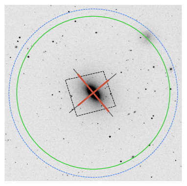
Figure 1: Image in the $R$ filter centred on NGC 3377, obtained through the ESO Digitized Sky Survey. The FOV is $16\times 16$ arcmin², and it follows the usual orientation (North is up, East to the left). The black dashed polygon represents the HST/ACS FOV. The thin grey lines correspond to the position and length of the long-slits observed through Gemini/GMOS-N, while the thick red ones highlight the radial range from which are measured the kinematical data. The green solid circle represents for comparison purposes the region containing the PNe from Coccato et al. (2009), and the blue dashed circle corresponds to GCs from Pota et al. (2013).

2.1 Surface brightness profile

For the surface brightness profile of NGC 3377, a Sérsic law (Sersic, 1968) is assumed, with the parameters fitted by Krajnović et al. (2013) to the $r$ filter, and converted to equivalent radius ($R_{\rm eq}$) with the axes ratio, $q_{\rm ab}=0.52$. The absorption in the $r$ filter is obtained from NED, and corresponds to $A_{r}=0.077$ mag, following the calibration by Schlafly & Finkbeiner (2011). In order to convert the units from mag arcsec^-2 to ${\rm L_{\odot}pc^{-2}}$, it is used $M_{r,\odot}=4.65$ mag (Willmer, 2018) for the absolute magnitude of the sun, and the distance already stated in Section 1. Hence, the expression results

$$I_{r}(R_{\rm eq})=I_{0}\,{\rm exp}\left[-\left(\frac{R_{\rm eq}}{R_{0}}\right)^{\frac{1}{n_{r}}}\right]$$ (1)

using the approximation of $b_{\rm n}$ from Ciotti (1991), with $n_{r}=5\pm 0.5$, $I_{0}=(1.184\pm 0.2)\times 10^{6}\,{\rm L_{\odot}pc^{-2}}$ and $R_{0}=0.023\pm 0.01$ pc. Further analysis in this paper requires to deproject the Sérsic law. Following the approximation from Prugniel & Simien (1997) and Lima Neto et al. (1999), see also Salinas et al. (2012), it results

$$\begin{split}j(x)&\simeq j_{1}\left(\frac{x}{R_{0}}\right)^{-p}{\rm exp}\left[-\left(\frac{x}{R_{0}}\right)^{\frac{1}{n_{r}}}\right],\\ j_{1}&=\frac{\Gamma(2n_{r})}{\Gamma\left[(3-p)n_{r}\right]}\frac{I_{0}}{R_{0}},\\ p&\simeq 1-\frac{1}{n_{r}}+\frac{0.05463}{n_{r}^{2}}\\ \end{split}$$ (2)

The stellar mass enclosed at a radius $x$ emerges from the integration of the previous expression and the mass-to-light ratio, which is assumed $M/L_{r}=3.55\pm 0.2$ by Cappellari et al. (2013b). For the cumulative luminosity, we follow Lima Neto et al. (1999),

$$\begin{split}L_{r}(x)&=L_{\rm tot}\frac{\gamma\left[(3-p)n_{r},(x/R_{0})^{\frac{1}{n_{r}}}\right]}{\Gamma\left[(3-p)n_{r}\right]},\\ L_{\rm tot}&=2\pi n_{r}\Gamma(2n_{r})I_{0}R_{0}^{2}\\ \end{split}$$ (3)

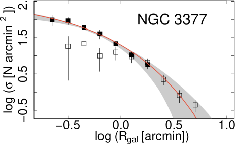
Figure 2: Projected radial distribution for the GCS of NGC 3377, corrected by completeness and contamination. The grey region represents the uncertainties in the Sérsic profile, and the red solid curve corresponds to the resulting fitting. The open symbols shows the projected density of the spectroscopically confirmed sample from Pota et al. (2013).

2.2 Globular clusters candidates

The photometric data set corresponds to a single field, centred on NGC 3377 (indicated with dashed lines in Fig. 1), and observed through the HST/ACS Wide Field Camera, during January 2006 (programme ID 10554). Both raw and processed images are available at the Mikulski Archive for Space Telescopes (MAST). These observations correspond to the filters $F475W$ and $F850LP$, commonly used in extragalactic GC studies, and the total exposure times are 1380 s and 3005 s, respectively. Its field-of-view (FOV) is $202\times 202$ arcsec².

In the following, the procedure for detecting and measuring the GC candidates is summarised. First, the diffuse galaxy light is subtracted in order to improve the detection of sources close to the galaxy centre in both filters. This is achieved by means of several tasks from iraf (version V2.16). First, elliptical isophotes are fitted to the galaxy in each filter using the task ELLIPSE. Bright stars and background galaxies on the field are masked to achieve a stable solution. The parameters ellipticity and position angle are simultaneously fitted for the inner $\approx 45$ arcsec. For larger galactocentric distances, the position angle is fixed to avoid fluctuations due to the low surface brightness level and the edges of the FOV. Then, this output is used to modelled the diffuse galaxy light with the task BMODEL, and finally subtracted to the original image. With the exception of some underlying features from the disk component in the inner 15 arcsec, the diffuse galaxy light is removed from the images. This procedure has proven to favour the detection of GC candidates in the inner regions of early-type galaxies in previous papers including ACS data (e.g. Caso et al., 2013, 2019; De Bórtoli et al., 2022). Afterwards, SExtractor (Bertin & Arnouts, 1996) is run in both filters to build up a preliminary catalogue of sources, assuming as a positive detection every group of at least three connected pixels with counts above the local sky level plus $3\sigma$. Although GCs at the assumed distance might be marginally resolved, from a typical effective radius of $\approx 3$ pc (e.g. Jordán et al., 2005; Brodie et al., 2011; Caso et al., 2014), and assuming low eccentricities (e.g. Harris, 2009), their full width at half-maximum (FWHM) should not exceed a few pixels. In order to reject extended sources, only those sources presenting FWHM smaller than 5 px and elongation smaller than 2 in both filters are selected, criteria also used in other studies with similar instrumental configuration and distances to the galaxies (e.g. Jordán et al., 2004, 2007). Aperture photometry is performed in both filters with an aperture radius of 5 px, and mean aperture corrections are calculated from the analysis of structural parameters of marginally resolved sources with ISHAPE (Larsen, 1999, see Caso et al. 2019 for further details). The photometry is calibrated to $g$ and $z$ filters, applying the zero-points from Sirianni et al. (2005), $ZP_{F475}=26.068$ and $ZP_{F850}=24.862$ mag. Then, the magnitudes are corrected by extinction, assuming the values from NED, $A_{g}=0.11$ mag and $A_{z}=0.04$ mag (Schlafly & Finkbeiner, 2011).

Finally, GC candidates are chosen from those sources with colours fulfilling $0.6<(g-z)_{0}<1.7$ mag, similar colour range than those assumed in previous GC studies using these bands (e.g. Jordán et al., 2005). Completeness functions for point-like sources are calculated from artificial stars in different galactocentric distances, to account for variations due to Poisson noise from the galaxy surface brigthness. Then, the faint limit for the photometric analysis is set at $z=24$ mag. This assures a high completeness level, and spans $\approx 95\%$ of the GCs, based on the GCs luminosity function from Cho et al. (2012). We refer to Caso et al. (2019) for further information about the calculus of the completeness correction for GC candidates in similar images.

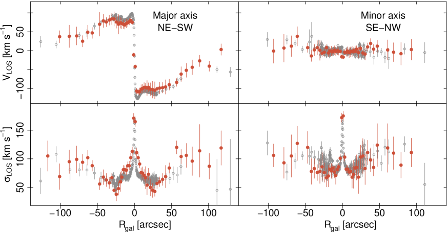
Figure 3: Long-slit stellar kinematics of NGC 3377, extracted along the photometric major (left-hand panels) and minor (right-hand panels) axes. The upper panels correspond to the velocity in the line-of-sight ($V_{\rm LOS}$), corrected by the systemic velocity of NGC 3377. The lower panels represent the velocity dispersions ($\sigma_{\rm LOS}$). For all panels, red filled circles indicate data presented in this paper, and grey open circles are from Coccato et al. (2009).

Figure 2 shows the radial distribution for the GCS of NGC 3377 as a function of the projected galactocentric distance ($R_{\rm gal}$), corrected by completeness and subtracted by contamination. The completeness corrections are obtained from completeness functions at four galactocentric ranges, to consider the changes on GCs detection as a consequence of the increasing noise close to the galaxy centre. The contamination is assumed $n_{\rm b}=1$ arcmin^-2, following Cho et al. (2012) for the same observations and photometric depth. The radial binning is constant on logarithmic scale, $log_{10}\Delta R{\rm{}_{gal}\,[arcsec]}=7$. A Sérsic profile (see Equation 1) is fitted for different bin breaks, slightly shifted to consider discreteness issues. The grey region in the figure represents the changes in the Sérsic profiles, while the red solid curve corresponds to the weighted mean of the parameters fitted in each individual run. These result $n_{\rm GCs}=3.1$, $I_{\rm 0,GCs}=3900$ arcmin^-2 and $R_{\rm 0,GCs}=0.0052$ arcmin. The open symbols double the projected density for the spectroscopically confirmed GCs brighter than $g^{\prime}=23$ mag, from Pota et al. (2013), for comparison purposes. This latter magnitude limit corresponds to the turn-over magnitude of the GCS, according to (Cho et al., 2012). For the outer region both profiles agree. The extension of the GC system (GCS) is assumed $7.5$ arcmin, that corresponds to the extension of the spectroscopic survey by Pota et al. (2013) and does not differ significantly from the extension of $6.2$ arcmin calculated by Caso et al. (2019). The numerical integration of this profile up to $7.5$ arcmin results $325\pm 30$ GCs, which doubles previous results from ACS studies (Cho et al., 2012).

2.3 Gemini/GMOS spectroscopy

Long-slit spectra of NGC 3377 has been observed with the Gemini Multi-Object Spectrograph (GMOS) mounted on Gemini North, during January/February in 2021 (GN-2020B-Q-401, PI Juan Pablo Caso). The aim of these observations was to complement data from the literature at large galactocentric distances (e.g. Coccato et al., 2009). Hence they were carried on relaxed observing conditions, with typical seeing of $\approx 2$ arcsec. The observations comprise two orientations, following the position angles for the photometric major and minor axes of the stellar component (PA$\approx 40\deg$ in the NE-SW direction, and PA$\approx 130\deg$ in the SE-NW direction, respectively, and represented with grey solid lines in Fig. 1). The observations are split in 16 exposures of 900 s each. The chosen grism is B600$\_$G5307, with a slit width of 1 arcsec, $2\times 2$ binning and central wavelengths in the range $5400-5550$ Å, to account for CCD gaps. The resulting spectral resolution is $\approx 6$ Å.

Both flatfields and CuAr lamps has been observed with each science image, to account for flexion effects. The standard reduction process is performed with the Gemini-GMOS routines in iraf (version V2.16). The two-dimensional spectra are spatially rebinned to achieve a $S/N\gtrsim 20$ at 5000 Å. Considering the typical seeing during the observations, the minimum spatial bin is set at 2 arcsec. The individual spectra are extracted in the wavelength range $4800-5800$ Å, that contains several absorption features typical of the spectra in elliptical galaxies (H$\beta$, Mgb, and Fe lines). The mean velocity and velocity dispersion in the line-of-sight are measured by means of the penalised Pixel Fitting code (ppxf, Cappellari & Emsellem, 2004; Cappellari, 2017). A subset of the MILES single stellar population models (Vazdekis et al., 2010) are selected as templates for ppxf fitting, considering old populations (8 and 10 Gyrs) and a wide range of metallicities (${\rm[Z/H]=}$ -1.31, -0.71, -0.4 and 0.0). The results for both slit orientations are listed in Table 2 at the Appendix. For the long-slit corresponding to the major axis of NGC 3377, kinematical measurements are obtained up to $\approx 2$ arcmin, and up to $\approx 1.6$ arcmin for the minor one. Both radial ranges are represented by red thick lines in Figure 1.

Figure 3 shows the velocity ($V_{\rm LOS}$) and velocity dispersion in the line-of-sight ($\sigma_{\rm LOS}$) as a function of $R_{\rm gal}$, expressed in arcsec, for the major (left-hand panels) and minor axes (right-hand panels). Filled red circles correspond to this paper. For comparison purposes, grey open symbols refer to the previous kinematical analysis performed by Coccato et al. (2009). The measurements from both datasets are in acceptable agreement, taking into account uncertainties and the differences in the spatial binwidth for the inner 30 arcsec. From a systemic $V_{\rm LOS}$ for NGC 3377 of $690\pm 5$ km s^-1 (Cappellari et al., 2011), the rotation velocity along the major axis achieves $\approx 100$ km s^-1 up to 40 arcsec from the galaxy centre, decreasing outwards. Besides, $\sigma_{\rm LOS}$ rapidly decreases from $\approx 180$ km s^-1 to a minimum of $\approx 60$ km s^-1 at 40 arcsec, to increase up to $\approx 100$ km s^-1 in the outskirts. On the contrary, along the minor axis $V_{\rm LOS}$ experiences a flatten distribution, and the profile of $\sigma_{\rm LOS}$ is soften. From these, Coccato et al. (2009) conclude that the galaxy presents a disc-like kinematics in the inner $\approx 60$ arcsec, with a larger contribution of the bulge, dynamically hotter, along the minor axis.

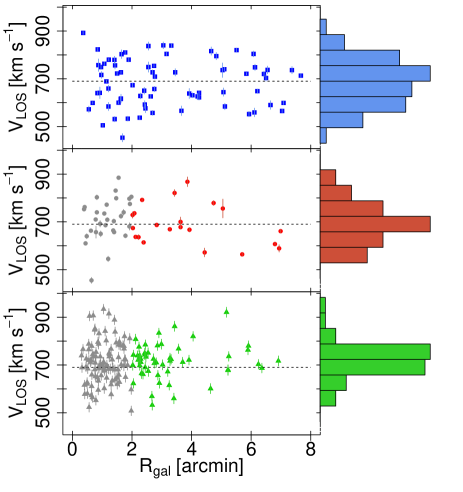
Figure 4: Velocity in the line-of-sight ($V_{\rm LOS}$) as a function of the galactocentric distance ($R_{\rm gal}$) for blue (upper panel) and red GCs (middle panel), and PNe (lower panel). The horizontal dashed line corresponds to the systemic $V_{\rm LOS}$ of NGC 3377. The objects in grey colour are not used in the present work due to signs of rotation.

2.4 Other kinematical sources

From the SLUGGS survey, Pota et al. (2013) present 126 spectroscopically confirmed GCs for NGC 3377. The sample spans up to $\approx 7.5$ arcmin from the galaxy centre (represented by the blue dashed circle in Fig. 1), and their uncertainties are typically ${\rm\approx 5-15\,km\,s^{-1}}$. The authors indicate that blue GCs do not present evidence of rotation, but red GCs are consistent with a rotation velocity $\approx 50-60$ km s^-1. For $R_{\rm gal}$ larger than 2 arcmin, the evidence for rotation becomes less accurate due to the size of the sample and the bias estimation presented for the method in their appendix. In this paper, the colour limit for blue and red GCs is assumed at $(g-i)=0.9$. The upper panel from Figure 4 shows the $V_{\rm LOS}$ for blue GCs as a function of $R_{\rm gal}$, while the middle panel is analogue for red GC. For the latter ones, only objects presenting $R_{\rm gal}>2$ arcmin are used in this study. Outlier objects are rejected iteratively, considering a $3\sigma$ criteria. Then, the final sample of GCs contains 93 objects, and its mean $V_{\rm LOS}$ results $685\pm 9$ km s^-1, which matches with the systemic $V_{\rm LOS}$ of NGC 3377. Following the adjusted Fisher-Pearson estimator for the kurtosis excess (Joanes & Gill, 1998), it results $-0.8\pm 0.4$. The uncertainty is approximated under the assumption of normality.

The planetary nebulae (PNe) in NGC 3377 have been studied by Coccato et al. (2009), resulting in a spectroscopically confirmed sample of 154 objects up to $\approx 6$ arcmin (represented by the green solid circle in Fig. 1). They also indicate evidence of rotation in the PNe population, with rotation velocity and kinematic position angle in agreement with the stellar population of the galaxy. For galactocentric distances larger than 2 arcmin, the mean velocity rotation seems to decrease to values consistent with zero in both the major and minor axes (see Figure 7 from Coccato et al., 2009). Then, those PNe presenting $R_{\rm gal}>2$ arcmin are selected for the present study. After the rejection of outliers, the sample consists of 53 objects with a mean $V_{\rm LOS}$ of $711\pm 14$ km s^-1. The kurtosis excess and its approximated uncertainty result $0.8\pm 0.6$. The mean $V_{\rm LOS}$ of the PNe differs from the systemic velocity of NGC 3377 in $\Delta V_{\rm LOS}=21\pm 15$ km s^-1, and in $\Delta V_{\rm LOS}=26\pm 17$ km s^-1 from the mean $V_{\rm LOS}$ of the CGs. A revision of both samples do not lead to any particular feature to explain this differences. In the range $2<R_{\rm gal}<2.5$ arcmin, 16 of 20 PNe present $V_{\rm LOS}$ larger than $690$ km s^-1, but the distribution of their position angles does not seem to follow the rotation of the inner disk. A thousand Monte-Carlo simulations are run, for normal samples with equal mean, dispersion in the range of $75-85$ km s^-1, and sizes corresponding to those of GCs and PNe samples used in the present work. Observational uncertainties are added to the objects, following the observed ones. It results in $\approx 12$ per cent of the cases presenting $\Delta V_{\rm LOS}>25$ km s^-1. Then, it cannot be concluded that the result implies some systematic difference between both samples.

2.5 Dark matter haloes from a numerical simulation

It is also used the cosmological dark matter simulation MDPL2, part of the Multidark project (Klypin et al., 2016, and publicly available through the official database of the project). This simulation spans a periodic cubic volume of $1\,h^{-1}\,{\rm Gpc}$ of size length. It contains $3840^{3}$ particles with mass of $1.51\times 10^{9}\,h^{-1}\,{\rm M_{\odot}}$ and it considers the cosmological parameters of Planck Collaboration et al. (2014). The dataset consists of the catalogue of dark matter haloes detected with the rockstar halo finder (Behroozi et al., 2013) in the snapshot that corresponds to the local Universe ($z=0$). Each halo is assumed to be the host of a unique galaxy, with the main halo hosting the central galaxy of each system, while the satellite haloes host the satellite galaxies.

In addition to the properties described in the catalogue, a luminosity in the $r$ band is assigned to each halo in a non parametric way, by means of a halo occupation distribution method (HOD Vale & Ostriker, 2006; Conroy et al., 2006). Under the assumption of a monotonic relation between the galaxy luminosities and the halo virial masses, the number density of haloes in a mass range match the number density of galaxies in the analogue luminosity range. While the first quantity is obtained from the simulation, the latter one follows the galaxy luminosity function (LF), described through a Schechter function (Schechter, 1976). The parameters of the LF correspond to the fits available in Lan et al. (2016), that discriminate between central and satellite galaxies. The $M_{r}$ magnitudes are assigned in decreasing order of luminosity, assuming a constant step of $0.01$ mag. Observational and numerical studies have pointed in the literature to an intrinsic scatter in the stellar-to-halo mass relation (SHMR, e.g. Erfanianfar et al., 2019; Legrand et al., 2019; Moster et al., 2010), that is usually represented by a log-normal distribution. Although the dependence with halo mass has been pointed by some authors (e.g. Matthee et al., 2017), in this work is assumed a constant scatter of $0.20$ following Girelli et al. (2020). Hence, the final $M_{r}$ magnitudes for the haloes account for this scatter through the latter expression. We are aware that inclusion of baryonic matter leads to some tension between cosmological simulations and observations from the Local Group in the low mass regime (Webb & Bovy, 2020, and references there in), but the expected mass for NGC 3377 is beyond this range.

Finally, the morphological type of the galaxy hosted in each halo is randomly selected between early and late type, on the bases of the red fraction of galaxies in different environments from McNaught-Roberts et al. (2014). To do so, a numerical density is calculated for each halo, $n_{\rm neig}$, defined as the number of neighbours closer than $8\,h$ Mpc that present luminosities brighter than $M_{r,{\rm lim}}=-20.1+5\,{\rm log_{10}}(h)$, i.e. $M_{r,{\rm lim}}=-21$ mag, due to completeness effects in the sample of McNaught-Roberts et al. (2014). Third-order polynomials are fitted to the fraction of red galaxies as a function of $M_{r}$ (see Figure 11 from McNaught-Roberts et al., 2014, and Figure 5 in this paper),

$$\begin{split}F_{\rm red}(x)&=44.5+7.48x+0.41x^{2}+0.01x^{3},\,{\rm for}\,\delta<0\\ &=44.1+7.26x+0.39x^{2}+0.01x^{3}\,{\rm for}\,0<\delta<4\\ &=45.9+7.41x+0.39x^{2}+0.01x^{3}\,{\rm for}\,\delta>4\\ \end{split}$$ (4)

with $x$ corresponding to the $M_{r}$ assigned to each halo, and $\delta$ to the environmental density, $n_{\rm neig},$ normalised by its mean value, $\delta=(n_{\rm neig}-\overline{n_{\rm neig}})/\overline{n_{\rm neig}}$

These polynomials and the previously derived numerical densities are used to separate the haloes hosting red and blue galaxies, as a proxy of early and late-type ones.

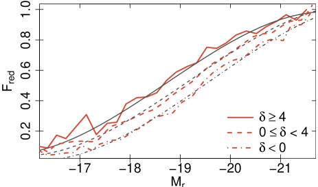
Figure 5: Fraction of red galaxies from McNaught-Roberts et al. (2014) as a function of $M_{r}$ (thick red lines) and third-order polynomials fitted to these relations (thin grey curves), for three different ranges of environmental density. The parameter $\delta$ corresponds to the normalised density of neighbours brighter than $M_{r,{\rm lim}}=-21$ mag (see text).

3 Dynamical modeling

3.1 Spherical Jeans analysis

Previous dynamical analysis up to the effective radius (Cappellari et al., 2013a, b) assumes axisymmetric models for NGC 3377, which is classified as a fast rotator at that radial range. In this case, we adopt a different scenario for the outskirts of the galaxy, based on both spectroscopical and photometrical data. In Section 2.3 it has been already noticed that the behaviour of $V_{\rm LOS}$ and $\sigma_{\rm LOS}$ along the major axis outwards 40 arcsec points to a decreasing contribution of the disc component. Arnold et al. (2014) analyse the two-dimensional photometry of NGC 3377, resulting in boxy isophotes and decreasing ellipticity outwards $\approx 30$ arcsec. The authors decompose the galaxy surface brightness profile into three components, pointing to an increasing contribution of the bulge for galactocentric distances larger than $\approx 30$ arcsec. Assuming constant velocity rotations for each component, it leads that the kinematics of the slow-rotating bulge dominates over the inner disk outwards $60-70$ arcsec. Then, we assume that outwards 60 arcsec of galactocentric distance, NGC 3377 behaves as a non-rotating systems with spherical symmetry, and the results from (Cappellari et al., 2013a, b) for the inner region are considered as constraints for the prior distribution (see Section 3.2.1). On the basis of the previous assumptions, the second-order velocity moments are related by the Jeans equation, (e.g. Łokas, 2002; Binney & Tremaine, 2008), resulting:

$$\frac{d\left[j(r){\sigma_{r}}^{2}(r)\right]}{dr}+\frac{2\beta}{r}j(r){\sigma^{2}_{r}}(r)=-j(r)\frac{GM(r)}{r^{2}}$$ (5)

with $j(r)$ as the three-dimensional density of the tracer population, $\beta$ is the anisotropy parameter, that accounts for possible departures from pure isotropy ($\beta>0$ for radial orbits, and $\beta<0$ for tangential ones), ${\sigma_{r}}^{2}(r)$ is the radial component of the velocity dispersion at the spatial galactocentric distance $r$, and $M(r)$ is the enclosed total mass. In the case of the fourth-order moments, additional assumptions are needed to constraint the solutions. Adopting a distribution function of the form $f(E,L)=f_{0}(E)L^{-2\beta}$, with constant anisotropy parameter, the ratio of the fourth-order moments are related with $\beta$, and the Jeans equations are reduced to a single one of the form (Łokas 2002, see also Richardson & Fairbairn 2013):

$$\frac{d\left[j(r)\overline{{V_{r}}^{4}}(r)\right]}{dr}+\frac{2\beta}{r}j(r)\overline{{V^{4}_{r}}}(r)=-3j(r)\sigma^{2}_{r}\frac{GM(r)}{r^{2}}$$ (6)

with $\overline{{V_{r}}^{4}}(r)$ the radial component of the fourth-order moment of the velocity. Then, the solution to previous equations, assuming constant $\beta$, reads:

$$j(r){\sigma_{r}}^{2}(r)=\int_{r}^{\infty}j(s)\frac{G\,M(s)}{s^{2}}\left(\frac{s}{r}\right)^{2\beta}ds$$ (7)

$$j(r)\overline{{V_{r}}^{4}}(r)=3\int_{r}^{\infty}j(s){\sigma_{r}}^{2}(s)\frac{G\,M(s)}{s^{2}}\left(\frac{s}{r}\right)^{2\beta}ds$$ (8)

From the observational perspective, the projections of the velocity moments represent more useful parameters, leading to direct comparison with measurable kinematics. The integration along the line-of-sight results:

$$\sigma_{\rm LOS}^{2}(R)=\frac{2}{n(R)}\int_{R}^{\infty}\left(1-\beta\frac{R^{2}}{r^{2}}\right)\frac{j\sigma_{r}^{2}rdr}{\sqrt{r^{2}-R^{2}}}$$ (9)

$$\overline{V_{\rm LOS}^{4}}(R)=\frac{2}{n(R)}\int_{R}^{\infty}\left[1-2\beta\frac{R^{2}}{r^{2}}+\frac{\beta(1+\beta)}{2}\frac{R^{4}}{r^{4}}\right]\frac{j\overline{V_{r}^{4}}rdr}{\sqrt{r^{2}-R^{2}}}$$ (10)

with $\sigma_{\rm LOS}(R)$ and $\overline{V_{\rm LOS}^{4}}(R)$ the second and fourth-order moments in the line-of-sight, respectively, $n(R)$ the projected density of the tracer population, and $R$ the projected radius. To simplify the previous expressions, it is avoided to make explicit the dependence on the three dimensional radius, $r$, of the stellar density and the moments of the velocity. Introducing Equation 7 into 9 and inverting the order of integration, it yields the integral solution

$$\sigma_{\rm LOS}^{2}(R)=\frac{2}{n(R)}\int_{R}^{\infty}K(R,r)j(r)M(r)\frac{dr}{r}$$ (11)

where the kernels $K(R,r)$ vary for different values of constant anisotropy, as indicated at the Appendix from Mamon & Łokas (2005). From Equations 7 and 8, Equation 10 results in a triple integral. Inverting the order of integration and rearranging the factors, it is obtained a solution of the form:

$$\begin{split}\overline{V_{\rm LOS}^{4}}(R)&=\frac{2}{I(R)}\int_{R}^{\infty}du\,G\,M(u)\,j(u)\,r^{2\beta-2}\\ &\int_{R}^{u}\,ds\frac{G\,M(s)}{s}s^{-2\beta}\,K^{4}({R,s})\\ \end{split}$$ (12)

with analogue kernels $K^{4}(R,s)$, presented at the Appendix A for constant anisotropy, ranging $-1/2\leq\beta\leq 1/2$.

3.2 Bayesian treatment

This work applies a Bayesian approach to estimate the mass profile of the galaxy. The components of the observational dataset $D$ have been already described in Section 2. It can be split in the density profiles of the tracer populations, $D_{\rm rad}=\{n_{\rm Gal},n_{\rm GCs}\}$, and the kinematical data, $D_{\rm kin}\,=\,\{{\rm Gal,GCs,PNe}\}$.

Several popular models used to describe dark matter haloes with spherical symmetry can be described by two parameters (e.g. Burkert, 1995; Navarro et al., 1997), typically a scale radius and a density or concentration parameter, for instance $r^{\prime},\rho^{\prime}$. Hence, the Bayesian analysis points to finding the probability $p\left(r^{\prime},\rho^{\prime}|D,I_{\rm prior}\right)$, with $I_{\rm prior}$ representing the information not included in the dataset that will mould the prior distribution. From the Bayes theorem,

$$p\left(r^{\prime},\rho^{\prime}|D,I_{\rm prior}\right)=\frac{p\left(r^{\prime},\rho^{\prime}|I_{\rm prior}\right)\,p\left(D|r^{\prime},\rho^{\prime},I_{\rm prior}\right)}{p\left(D|I_{\rm prior}\right)}$$ (13)

the probability $p\left(D|I_{\rm prior}\right)$ is considered as a normalisation factor, and its determination is avoided, while the factor $p\left(r^{\prime},\rho^{\prime}|I_{prior}\right)$ correspond to the prior distribution. The second factor in the equation can be factorised as

$$\begin{split}p\left(D_{\rm kin}|r^{\prime},\rho^{\prime},D_{\rm rad},I_{\rm prior}\right)&=p\left(Gal|r^{\prime},\rho^{\prime},D_{\rm rad},I_{\rm prior}\right){\bf\cdot}\\ &\quad p\left(GCs|r^{\prime},\rho^{\prime},D_{\rm rad},I_{\rm prior}\right){\bf\cdot}\\ &\quad p\left(PNe|r^{\prime},\rho^{\prime},D_{\rm rad},I_{\rm prior}\right)\end{split}$$ (14)

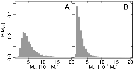
Figure 6: Distribution of virial masses ($M_{\rm vir}$)for dark matter haloes from the MDPL2 simulation, that results from the first constraint presented in Section 3.2.1, for central (case A, left panel) and satellite haloes (case B, right panel).

where $Gal$ represents the velocity dispersion profile of the stellar population of the galaxy, and its probability for a specific set of $r^{\prime},\rho^{\prime}$ is obtained through the $\chi^{2}$ distribution, from the expression

$$\chi^{2}=\sum_{j}\left(\frac{{\sigma^{\rm obs}_{\rm LOS,j}}-{\sigma^{\rm pred}_{\rm LOS,j}}}{{e\sigma^{\rm obs}_{\rm LOS,j}}}\right)^{2}$$ (15)

where ${\sigma^{\rm obs}_{\rm LOS,j}}$ represents the measurements of the velocity dispersion in the line-of-sight, already presented in Section 2.3, and ${e\sigma^{\rm obs}_{\rm LOS,j}}$ corresponds to the associated error. In the case of ${\sigma^{pred}_{\rm LOS,j}}$, it symbolises the value predicted by the model with parameters $r^{\prime},\rho^{\prime}$, and fixed anisotropy $\beta$. The sum is over the measurements at projected galactocentric distances ($R_{\rm gal}$) larger than 1 arcmin, for which rotation fades, and presenting ${e\sigma_{j}}^{\rm obs}$ smaller than 50 km s^-1.

The joint probability of the sample of GCs is obtained as the product of the individual probabilities for each object. These are obtained for each GC from the convolution of its observational $V_{\rm LOS}$ distribution, and the predicted one at the $R_{\rm gal}$. The first one is assumed as a Gaussian centred at the measured $V_{\rm LOS}$ with dispersion equal to the error of the measurement. The latter one is centred in the mean $V_{\rm LOS}$ of the sample, $685$ km s^-1, which agrees with the systemic velocity of the galaxy. It is expressed in terms of the Gauss-Hermite polynomials (van der Marel & Franx, 1993), with terms that characterise asymmetric deviations from the normal distribution vanishing based on the spherical symmetry,

$$f(w)=\frac{1}{\sqrt{2\pi}\sigma}{\rm exp}\left(-\frac{1}{2}w^{2}\right)\left[1+\frac{h_{4}}{\sqrt{24}}(4w^{4}-12w^{2}+3)\right]$$ (16)

plus higher-order terms which are assumed negligible in this approach, $w=(V_{\rm LOS}-V_{0})/\sigma_{\rm LOS}$ and $h_{4}$ is related with the fourth-order moment of the velocity in the line-of-sight by $h_{4}=(\overline{V_{\rm LOS}^{4}}/\sigma_{\rm LOS}^{4}-3)/(8\sqrt{6})$, with $\sigma_{\rm LOS}$ and $\overline{V_{\rm LOS}^{4}}$ arising from the Jeans analysis, for each pair of parameters $r^{\prime}$, $\rho^{\prime}$. The same treatment is applied to the PNe sample, but in this case the mean $V_{\rm LOS}$ from the sample results $711$ km s^-1.

3.2.1 Prior distribution

The information in $I_{\rm prior}$ is based on two constraints for the halo parameters. The first one is built from the haloes in the MDPL2 simulation with absolute magnitudes in the $r$ filter consistent with the brightness of NGC 3377. The total apparent magnitude in the $r$ band for the galaxy is obtained from the integration of the surface brightness profile derived by Krajnović et al. (2013), and the extinction correction from Section 2.1. It results $r=10.11\pm 0.08$ mag. From the previous magnitude and the distance already presented in Section 1 (that implies a distance modulus of $m-M=30.13\pm 0.08$ mag), results the distribution of absolute magnitudes ($M_{r}$), which is used to statistically select haloes from the MDPL2 simulation, based on their resulting $M_{r}$ from the HOD method. Two scenarios of prior distribution are considered, in case (A) only central haloes are used to build it, and in case (B) only satellite haloes are taken into account. In Figure 6 are shown the distribution of virial masses ($M_{\rm vir}$) built from the haloes in the MDPL2 simulation for both scenarios (central and satellite haloes), i.e. $p(M_{\rm vir}|I_{\rm prior})$, that emerges from the first constraint. The two panels present the cases (A) and (B), achieving the 95-percentile at $M_{\rm vir}$ values of $10^{12}$ and $6\times 10^{11}\,{\rm M_{\odot}}$, respectively. The restriction to satellites favours less massive haloes due to the differences in the luminosity functions for central and satellite galaxies from Lan et al. (2016). This is expected as a consequence of the mass loss in subhaloes beyond their accretion, caused by dynamical friction, tidal stripping and tidal heating processes (e.g. Gan et al., 2010). In this regard, Cora et al. (2018) indicated for haloes less massive than $\approx 10^{12}\,{\rm M_{\odot}}$, that central galaxies inhabit more massive haloes than satellites at fixed stellar mass.

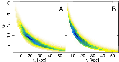
Figure 7: Prior distribution of the parameters describing the NFW profile, derived from both constraints in Section 3.2.1, for central haloes (case A, left panel) and satellite ones (case B, right panel). The colour gradient, from light yellow to dark blue, represents sets of parameters with increasing probability.

The second constraint comes from Cappellari et al. (2013a, b), who found for NGC 3377 dynamical and stellar mass-to-light ratios ($M/L_{r}$) corresponding to a dark matter fraction of $\approx 6\%$ up to $1\,R_{\rm eff}$, with errors for the fitted $M/L_{r}$ of $\approx 6\%$. Considering that both constraints apply on $M_{\rm vir}$, it results

$$p(r^{\prime},\rho^{\prime}|I_{\rm prior})=p(r^{\prime},\rho^{\prime}|M_{\rm vir})p(M_{\rm vir}|I_{\rm prior})$$ (17)

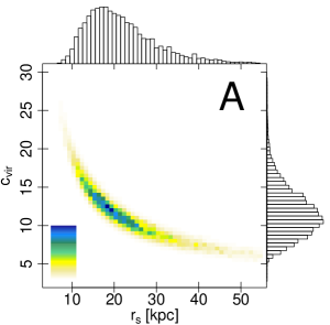
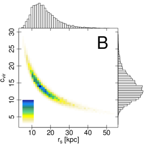
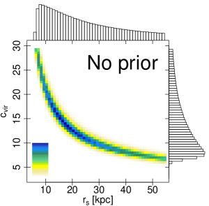
Figure 8: Colour map of the NFW profiles for the joint probability of the stellar population, GCs and PNe, when different anisotropy parameters are assumed for each tracer population ($\beta_{\rm GCs}=-0.5$, $\beta_{\rm stel}=0$ and $\beta_{\rm PNe}=0.5$). The NFW profile is described in terms of the concentration parameter ($c_{\rm vir}$) and its characteristic radius ($r_{\rm s}$). The colour gradient evolves from light yellow to dark blue, representing increasing joint probabilities. The three panels differ in the prior distribution, built from central haloes (case A, left panel), satellite haloes (case B, middle panel), and no prior (right panel). The side histograms correspond to the marginal distributions for $c_{\rm vir}$ and $r_{\rm s}$.

4 Results

In this Section are presented the results obtained from the analysis already described in Section 3, based on the observational dataset gather in this paper, and presented in Section 2. A cuspy mass distribution is assumed, applying both the NFW and Einasto models. Although core-like halo distributions accurately represent the mass profile in dwarf galaxies, it is not clear whether the haloes from galaxies in the mass range of NGC 3377 significantly deviate from the inner slopes represented by the assumed profiles (e.g. Del Popolo, 2016; Oh et al., 2015). Also the scenarios in which NGC 3377 behaves as a central or satellite halo are considered to define the prior distribution (see Section 3.2.1 for further details), as well as several cases of constant anisotropy ($\beta$).

4.1 The NFW profile

The NFW profile (Navarro et al., 1997), commonly used for modelling dark matter haloes, can be described by a characteristic radius ($r_{\rm s}$) and density ($\rho_{\rm s}$). The mass profile in terms of these two parameters is

$$M_{\rm NFW}(r)=4\pi\rho_{\rm s}r^{3}_{\rm s}\left[ln\left(1+r/r_{\rm s}\right)-\frac{r/r_{\rm s}}{1+r/r_{\rm s}}\right]$$ (18)

Following the definitions from Bullock et al. (2001), the concentration parameter is the ratio between the virial ($R_{\rm vir}$) and characteristic radii, $c_{\rm vir}=R_{\rm vir}/r_{\rm s}$, with $R_{\rm vir}$ the radius at which the mean density within it equals to $\Delta_{\rm vir}(\Omega_{\rm m})$ times the mean matter density ($\rho_{\rm m}$). For $\Omega_{\rm m}=0.307$ and the approximation from Bryan & Norman (1998), it results $\Delta_{\rm vir}\approx 333$. From the definition of the density parameter $\Omega_{\rm m}$, it results $\rho_{\rm m}=\Omega_{\rm m}\rho_{\rm crit}$, where the last factor corresponds to the critical density for a flat Universe, $\rho_{\rm crit}=3H^{2}_{0}/(8\pi G)$. Then, it leads to a relation involving $\rho_{\rm s}$ and $c_{\rm vir}$

$$\rho_{\rm s}=100\frac{H^{2}_{0}}{8\pi G}\frac{c^{3}_{\rm vir}}{ln(1+c_{\rm vir})-c_{\rm vir}/(1+c_{\rm vir})}$$ (19)

with $H_{0}=67.77$ km s^-1 Mpc^-1 and $G$ the gravitational constant. Then, the expression for the virial mass of a NFW halo directly arises, from these equations and the definition of $c_{\rm vir}$, $M_{\rm vir}=51.1H^{2}_{0}(c_{\rm vir}r_{\rm s})^{3}/G$

Hereafter, the parameters $r_{\rm s}$ and $c_{\rm vir}$ describes the NFW profile, instead of $\rho_{\rm s}$. In Figure 7 is shown the prior distribution derived from both restrictions on the $M_{\rm vir}$, presented in Section 3.2.1, and applied to the NFW parameters. The colour gradient ranges from light yellow to dark blue towards pairs of $(r_{\rm s},c_{\rm vir})$ with larger probability. The panels correspond to central and satellite haloes.

Table 1: Solutions for the kinematical analysis from the three sets of tracers, i.e. stellar population, GCs and PNe. For each parameter of the density distribution, the mode, mean and dispersion are indicated in three consecutive columns. Two anisotropy options are assumed, in the first one the isotropic case is applied for the three sets of tracers, and the second option considered different anisotropy parameters for each set (see text in Section 4.1). For each anisotropy option, the solutions listed in consecutive rows differ in the prior distribution, built from central haloes (case A), satellite haloes (case B), or no prior distribution (third row). In these latter cases, the large dispersion in the distribution of joint probabilities prevent us from indicating the modes of the parameters. The distribution parameters are $r_{\rm{\rm s}}$ and $c_{\rm vir}$ for the NFW profile, and $r_{-2}$ and $\rho_{-2}$ in the case of the Einasto profile. In this latter case, the third parameter is fixed at $n=8$ (further details in the text). For both density distributions, also the $M_{\rm vir}$ estimators are shown in the last three columns.

NFW profile
Prior	$r_{\rm s}{\rm[kpc]}$			$c_{\rm vir}$			$M_{\rm vir}{\rm[10^{11}\,M_{\odot}]}$
$\beta=0.0$
A	$18\pm 2.7$	$21.4\pm 2.5$	$8.3\pm 1.0$	$12.5\pm 1.5$	$12.2\pm 1.1$	$3.1\pm 0.2$	$4.1\pm 1.1$	$6.1\pm 1.1$	$2.6\pm 0.5$
B	$15\pm 2.5$	$18.0\pm 2.3$	$7.1\pm 1.0$	$13.5\pm 1.5$	$13.5\pm 1.0$	$3.5\pm 0.3$	$3.6\pm 0.9$	$4.9\pm 1.2$	$2.1\pm 0.5$
-	$-$	$24.1\pm 5.1$	$13.2\pm 1.5$	$-$	$13.7\pm 2.3$	$5.7\pm 0.7$	$-$	$6.3\pm 1.9$	$4.2\pm 1.3$
$\beta_{\rm GCs}=-0.5$, $\beta_{\rm stel}=0.0$, $\beta_{\rm PNe}=0.5$
A	$18\pm 3.1$	$22.1\pm 2.5$	$8.7\pm 1.1$	$12.5\pm 1.7$	$12.4\pm 1.2$	$3.1\pm 0.2$	$4.1\pm 1.0$	$5.8\pm 1.1$	$2.4\pm 0.5$
B	$14\pm 2.5$	$17.0\pm 2.3$	$6.9\pm 1.0$	$14.0\pm 1.4$	$13.5\pm 1.1$	$3.5\pm 0.3$	$3.6\pm 0.9$	$4.6\pm 1.1$	$2.0\pm 0.5$
-	$-$	$24.1\pm 5.4$	$13.2\pm 1.3$	$-$	$13.5\pm 2.6$	$5.6\pm 0.7$	$-$	$6.3\pm 1.7$	$4.1\pm 1.2$
Einasto profile
Prior	$r_{-2}{\rm[kpc]}$			$\rho_{-2}{\rm[10^{-3}\,M_{\odot}\,pc^{-3}]}$			$M_{\rm vir}{\rm[10^{11}\,M_{\odot}]}$
$\beta=0.0$
A	$17\pm 4.2$	$19.8\pm 2.8$	$9.0\pm 0.7$	$1.0\pm 0.2$	$1.3\pm 0.2$	$0.9\pm 0.1$	$4.4\pm 2.2$	$5.6\pm 2.0$	$2.1\pm 0.7$
B	$12\pm 3.5$	$16.6\pm 2.7$	$7.5\pm 0.8$	$1.8\pm 0.4$	$1.7\pm 0.2$	$1.1\pm 0.1$	$3.8\pm 1.6$	$4.7\pm 1.9$	$1.7\pm 0.7$
-	$-$	$17.7\pm 1.8$	$9.3\pm 1.4$	$-$	$2.2\pm 0.3$	$1.4\pm 0.1$	$-$	$7.1\pm 2.1$	$2.7\pm 0.5$
$\beta_{\rm GCs}=-0.5$, $\beta_{\rm stel}=0.0$, $\beta_{\rm PNe}=0.5$
A	$22\pm 4.1$	$19.5\pm 2.8$	$8.9\pm 0.7$	$0.6\pm 0.2$	$1.2\pm 0.2$	$0.9\pm 0.1$	$4.3\pm 1.9$	$5.1\pm 2.0$	$1.9\pm 0.8$
B	$12\pm 3.4$	$15.8\pm 2.8$	$7.5\pm 0.8$	$1.8\pm 0.3$	$1.5\pm 0.2$	$1.1\pm 0.1$	$3.3\pm 1.5$	$4.2\pm 1.9$	$1.5\pm 0.7$
-	$-$	$17.8\pm 2.0$	$9.9\pm 1.5$	$-$	$2.1\pm 0.4$	$1.4\pm 0.1$	$-$	$6.2\pm 2.0$	$2.5\pm 0.5$

Following Equation 13, the joint probability for each pair of parameters $(r_{\rm s},c_{\rm vir})$ results from the product of Equations 14 and 17, with the latter one changing for cases (A) and (B), and the former equation depending on the orbital anisotropy ($\beta$). Although more complex treatments for this parameter are derived in the literature (e.g. Mamon & Łokas, 2005), in this paper only solutions with constant anisotropy are considered. The degeneracy between solutions with different values of $\beta$ might be partially resolved analysing the kurtosis of the velocity distribution for the stellar component (Napolitano et al., 2009; Salinas et al., 2012) and the estimators from Section 2.4. The appendix C in Coccato et al. (2009) shows the distribution of $h4$ parameter for the major and minor axis of NGC 3377, the values are consistent with kurtosis $\approx 0$ between 60 and 120 arcsec, but the data points are scarce and the uncertainties are large. The $\beta$ parameter up to the effective radius for a sample of elongated ellipticals from the SAURON project (Cappellari et al., 2007) span from $\approx-0.2$ to $\approx+0.2$, with NGC 3377 being nearly isotropic (see their Table 2).

The first rows in Table 1 shows the mode, mean and dispersion for the distributions of $r_{\rm s}$ and $c_{\rm vir})$, for the isotropic case ($\beta=0$) and the three options regarding the prior distribution (i.e., central haloes, satellite haloes, and no prior). Also the parameters for the distribution of $M_{\rm vir}$ are indicated in the last three columns. In the cases of no prior distribution, the large dispersion in the distribution of joint probabilities prevent us from indicating the modes of the parameters. The uncertainties come from the parameters dispersion from 100 Monte-Carlo realisations on artificial samples, generated to represent the observational data set and its uncertainties (see Section 4.3). Also a set of mild constant anisotropies, ranging from $\beta=-0.5$ to $\beta=0.5$ have been used. These results are consistent, with modes and means pointing to more massive (modes of $M_{\rm vir}$ ranging from $3.4\pm 1.0$ to $6.1\pm 1.2\times 10^{11}\,{\rm M_{\odot}}$ for central haloes and from $2.9\pm 0.9$ to $5.4\pm 0.9\times 10^{11}\,{\rm M_{\odot}}$ for satellites) and less concentrated haloes (modes of $c_{\rm vir}$ ranging from $11\pm 2$ to $13\pm 1.5$ for central haloes). The prior distribution restricted to satellite haloes favours less massive haloes than that for central ones, reflecting the differences that arise from the first constraint in Section 3.2.1. The last fitting option for the NFW profile in Table 1 corresponds to solutions that account for different anisotropy parameters for each kinematical tracer. For the stellar population is assumed the isotropic case ($\beta_{\rm stel}=0.0$), which does not contradict the $h_{4}$ measurements at Appendix C from Coccato et al. (2009) and Table 2 in Cappellari et al. (2007). The GCs kinematical data is fitted considering $\beta_{\rm GCs}=-0.5$, and $\beta_{\rm PNe}=0.5$ is assumed for the PNe. These values are based on the kurtosis estimators from Section 2.4. In Figure 8 are shown the distributions of the parameters $(r_{\rm s},c_{\rm vir})$ for this latter case, with the prior distributions corresponding to central haloes (case A, left panel), satellite haloes (case B, middle panel), and without prior distribution (right panel). The grid of parameters is built with steps $\Delta c_{\rm vir}=0.5$ and $\Delta r_{\rm s}=1$ kpc, and represents a wide range of $M_{\rm vir}$. The colour gradient ranges from light yellow to dark blue towards halo parameters $(r_{\rm s},c_{\rm vir})$ with larger joint probability, according to both the fit of the dynamical tracers and the prior distributions (in the cases that applies). The side histograms in each case correspond to the marginal distributions for $c_{\rm vir}$ and $r_{\rm s}$.

4.2 The Einasto profile

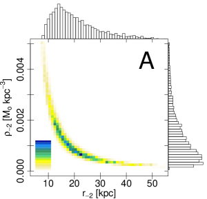
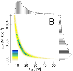
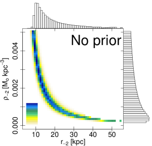
Figure 9: Colour map of the Einasto profiles for the joint probability of the stellar population, GCs and PNe, when different anisotropy parameters are assumed for each tracer population ($\beta_{\rm GCs}=-0.5$, $\beta_{\rm stel}=0$ and $\beta_{\rm PNe}=0.5$). The mass profile is described in terms of the characteristic radius ($r_{-2}$) and the mass density at this value ($\rho_{-2}$). The colour gradient represents increasing probability, from yellow to dark blue. The three panels differ in the prior distribution, built from central haloes (case A, left panel), satellite haloes (case B, middle panel), and no prior (right panel).

The Einasto profile (Einasto, 1965) has been useful to describe the density of dark matter haloes in numerical simulations, and its properties have been extensively analysed in the literature (e.g. Retana-Montenegro et al., 2012, and references there in). It possesses a power-law logarithmic slope, leading to the expression:

$$\rho_{\rm Ein}(r)=\rho_{-2}{\rm exp}\left\{-2n\left[\left(\frac{r}{r_{-2}}\right)^{1/n}-1\right]\right\}$$ (20)

with $r_{-2}$ acting as a characteristic radius where the density profile behaves as a power-law with exponent $-2$, $\rho_{-2}$ represents the density at this radius, and $n$ is a positive number reflecting the steepness of the power-law. The mass profile in terms of these parameters is

$$\begin{split}M_{\rm Ein}(r)&=M_{*}\gamma\left(3n,2n\sqrt[n]{\frac{r}{r_{-2}}}\right),\\ M_{*}&=4\pi\rho_{-2}r^{3}_{-2}n\frac{e^{2n}}{(2n)^{3n}}\\ \end{split}$$ (21)

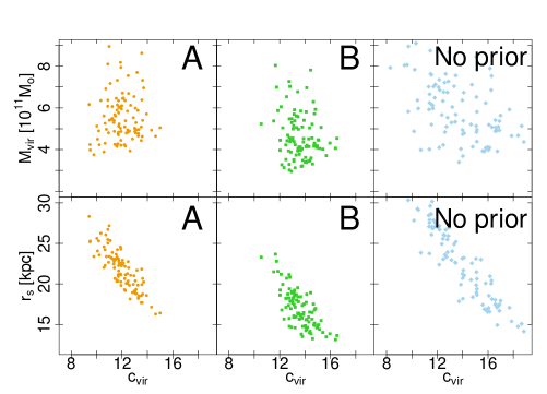
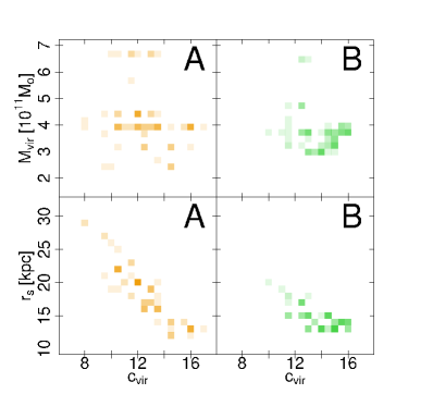
Figure 10: Left panels: Means of the distributions of parameters for the NFW profile, obtained in the same manner than those from the observational dataset, for 100 Monte-Carlo realisations when different anisotropy parameters are assumed for each tracer population ($\beta_{\rm GCs}=-0.5$, $\beta_{\rm stel}=0$ and $\beta_{\rm PNe}=0.5$). The three options differ in the prior distribution, assuming central haloes (case A), satellite haloes (case B), and no prior distribution. Right panels: Modes of the distributions of parameters from 100 Monte-Carlo realisations, obtained for the same anisotropy case and the NFW profile. The colour gradients, increasing from light to dark, represents more repeated sets of parameters. Only cases A and B are presented this time.

with $\gamma(a,x)$ corresponding to the lower incomplete gamma function. Its $R_{\rm vir}$ is derived from this latter expression and its definition, looking for the value $R_{\rm vir}$ that leads to a mean density in the halo that equals $333$ times the mean matter density ($\rho_{\rm m}$, see Section 4.1). Then, evaluating the previous equation at $R_{\rm vir}$ leads to the virial mass, $M_{\rm vir}$. Defining $\alpha=n^{-1}$, Gao et al. (2008) found that $\alpha$ is related with the halo mass and the redshift through the rms fluctuation of the density field $\sigma(M,z)$, varying very little for present day haloes with masses below $10^{13}\,{\rm M_{\odot}}$. A similar relation was fitted by Klypin et al. (2016) from the suite of Multidark cosmological simulations. From this latter relation, it is assumed $\alpha=0.125$ for the range of virial masses expected for NGC 3377, resulting in $n=8$. Then, the profile is described by only two free parameters, $r_{-2}$, and $\rho_{-2}$, for whom the prior distributions are built from the two constraints presented in Section 3.2.1, in the same manner than those for the NFW profile.

The lower half of Table 1 lists the mode, mean and dispersion for the free parameters of the Einasto profile, and for the $M_{\rm vir}$ distribution, when the prior distribution is derived from the central haloes population (case A) or from the satellite haloes one (case B), and also the results for no prior distribution at all (third row). In these latter cases, the large dispersion in the distribution of joint probabilities prevent us from indicating the modes of the parameters. The uncertainties are obtained from 100 Monte-Carlo realisations that reproduced the sizes and errors of the observational data set (see Section 4.3). In the first option, it is shown the isotropic case for the three tracer populations, although a larger set of anisotropy parameters (from $\beta=-0.5$ to 0.5) are considered. Increasing $\beta$ values result in more massive haloes (the mode of $M_{\rm vir}$ ranges from $4.3\pm 1.7$ to $7.8\pm 2.6\,{\rm M_{\odot}}$ for central haloes, and from $3.3\pm 1.5$ to $6.8\pm 2.4\,{\rm M_{\odot}}$ for satellites), with density profiles that steepen at larger radii (the mode of $r_{-2}$ ranges from $20\pm 4.0$ to $25\pm 4.5$ kpc for central haloes, and from $11\pm 3.4$ to $22\pm 4$ kpc for satellites). This behaviour is similar to that derived from NFW profiles in the previous section. Also a solution with different choices of $\beta$ parameters for each tracer population (i.e. $\beta_{\rm stel}=0.0$ for the stellar population, $\beta_{\rm GCs}=-0.5$ for the GCs, and $\beta_{\rm PNe}=0.5$ for the PNe) is applied, analogue to the NFW analysis. As expected, in all cases the prior distribution derived from satellite haloes leads to lighter haloes. The distributions of the parameters $(r_{-2},\rho_{-2})$ for the latter anisotropy case are shown in Figure 9. The three panels represent the results when the prior distributions correspond to cases (A) and (B), as well as the results whether no prior distribution is applied. For this profile, the steps of the grid of parameters are $\Delta r_{-2}=1$ kpc and $\Delta\rho_{-2}=10^{-4}\,{\rm M_{\odot}\,pc^{-3}}$. The colour gradient ranges from light yellow to dark blue towards halo parameters $(r_{-2},\rho_{-2})$ with larger joint probability. The side histograms in each case correspond to the marginal distributions for $r_{-2}$ and $\rho_{-2}$.

4.3 Testing the procedure

In order to test the accuracy of the procedure, 100 Monte-Carlo realisations are generated for each option of mass profile (i.e., NFW or Einasto), $\beta$ parameter, and prior distribution. In each case, the parameters that describe the respective mass profile of the haloes are assumed as those listed in Table 1. The size and galactocentric ranges of the artificial samples match those from the observational ones. Random velocity uncertainties are added to the simulated $V_{\rm LOS}$, following the percentile distribution of the velocity errors from the observational data set.

Once the artificial sample is generated, the procedure described in Section 3 is applied in the same manner than for the observational data set. In each step, the mode, mean and dispersion for the distribution of parameters of the mass profile, and the $M_{\rm vir}$ distribution are recorded. The results show a good agreement with the underlying set of parameters. In the left panels of Figure 10, the mean for the distributions of parameters in the case of different anisotropy parameter for each tracer population are plotted for the NFW profile, and the three options of prior distribution. When prior distributions are avoided, the 100 realisations leads to more dispersed results. After rejecting outliers, the 90-percentile of the mean values in cases (A) and (B) differs from the original parameters in less than 4 kpc for $r_{\rm s}$, 1.6 for $c_{\rm vir}$, and $1.7\times 10^{11}$ ${\rm M_{\odot}}$ for $M_{\rm vir}$, if NFW profiles are assumed. For the Einasto profiles, the 90-percentiles of the mean values are achieved at 5 kpc for $r_{-2}$, $3.8\times 10^{-4}\,{\rm M_{\odot}\,pc^{-3}}$, and $3\times 10^{11}\,{\rm M_{\odot}}$ for $M_{\rm vir}$. In the right panels of Figure 10 are plotted the distributions of modes for the NFW profile and the case of different anisotropy parameter for each tracer population. The colour gradients, increasing from light to dark, represent more repeated sets of parameters. Only cases A and B are showed this time. In comparison with the means of the parameters, the modes are typically more disperse, due to discreteness effects from the grid. For each parameter, the dispersion from these 100 realisations are used to estimate the uncertainties of the results listed in Table 1.

5 Comparison with the literature

Regarding the M 96 subgroup, it seems to be a moderately massive group of galaxies, with $M_{\rm vir}\approx 7\times 10^{12}\,{\rm M_{\odot}}$ (Karachentsev & Karachentseva, 2004), which implies a virial radius of $\approx 500$ kpc for a NFW profile. The mean harmonic distance for the galaxies is $\approx 190$ kpc, similar to the most probable $R_{\rm vir}$ for NGC 3377. From the radial velocities measured for a small sample of GCs, Bergond et al. (2006) obtained for NGC 3379, the other moderately bright elliptical, a velocity dispersion which is consistent with a halo presenting $M_{\rm vir}\approx 6\times 10^{11}\,{\rm M_{\odot}}$, which implies $R_{\rm vir}\approx 220$ kpc. The projected distance from NGC 3379 and M 96 to NGC 3377 are $\approx 1.4$ deg and $\approx 2.2$ deg, respectively, corresponding to $\approx 260$ kpc and $\approx 400$ kpc at NGC 3377 distance. From the mean distances calculated by NED, the difference in distances between NGC 3377 and these two galaxies are $\approx 100$ kpc and $\approx 300$ kpc for NGC 3379 and M 96, respectively. Tully et al. (2013) limited the distance estimators to surface brightness fluctuations, Cepheids and tip of the red-giant branch, leading to differences in distance of $\approx 600$ and $\approx 100$ kpc for NGC 3379 and M 96, respectively, which are lower than the fiducial 10 per-cent uncertainty for distance estimators. Although it is possible that NGC 3377 behaves as a main halo, the most probable scenario is that it belongs to the M 96 subgroup. Then, the solutions that correspond to case (B) in Table 1 are preferred. From these, the anisotropy parameters $\beta\pm 0.5$ hardly provide compatible results with the observational constraints for both GCs and PNe at the same time. For the remaining cases, the isotropic and that with different anisotropies for each kinematical tracers, the most probable haloes from the NFW profile are similar, and the weighted mean of their most probable virial masses leads to $(3.6\pm 0.6)\times 10^{11}\,{\rm M_{\odot}}$. Although the modes of the $M_{\rm vir}$ distributions for both anisotropy parameters differ in the case of the Einasto profile, their variation are enclosed by the uncertainties. The weighted mean results $(3.5\pm 1.1)\times 10^{11}{\rm M_{\odot}}$, in agreement with that derived from the NFW profile.

From Chandra observations, Kim & Fabbiano (2015) measure for the hot gas in NGC 3377 a temperature of ${T_{\rm GAS}}\approx 0.2$ keV and a luminosity in the range $0.3-8$ keV of ${L_{\rm X,GAS}}\approx 10^{38}\,{\rm ergs^{-1}}$. The relation derived by Forbes et al. (2017) for the ${L_{\rm X,GAS}}$ leads to a total mass up to five effective radii of ${M_{\rm tot}(<5\,R_{\rm eff})}$ $\approx(0.5-1)\times 10^{11}\,{\rm M_{\odot}}$. Similar results are obtained from the scaling relations fitted by Babyk et al. (2018) for ${L_{\rm X,GAS}}$ and ${T_{\rm GAS}}$. If the most probable parameters from Table 1 are used to calculate ${M_{\rm tot}(<5\,R_{\rm eff})}$, the results agrees with the ranges derived from the X-ray observations. These also agrees with the estimations up to $5\,{R_{\rm eff}}$ from Alabi et al. (2016).

From the $(B-V)$ colours and $K$ magnitudes from NED for the probable members of the M 96 subgroup, the relations derived by Bell et al. (2003) leads to stellar masses in the range $M_{\star}=(1.5-6)\times 10^{10}\,{\rm M_{\odot}}$, with $M_{\star}=2\times 10^{10}\,{\rm M_{\odot}}$ for NGC 3377. From the SHMR derived by Girelli et al. (2020), the cumulative virial mass is about $(5-8)\times$ $10^{12}\,{\rm M_{\odot}}$, in agreement with the estimation from Karachentsev & Karachentseva (2004). From this expression, the virial mass of NGC 3377 is $(6\pm 3)\times 10^{11}$ ${\rm M_{\odot}}$.

Hudson et al. (2014) analyse a compilation of galaxies with available information about the size of their GCS. From a SHMR derived from weak lensing analysis, they estimate halo masses and define a mean ratio between the mass enclosed in GCs and the halo mass, $\eta_{\rm M}={M_{\rm GCS}/M_{\rm vir}}$. This parameter seems to be independent on both the stellar and halo masses of the galaxy, and it results $\eta_{\rm M}\approx 4\times 10^{-5}$ with a large dispersion. From a different approach, Forbes et al. (2016) arrive to $\eta_{\rm M}\approx 3.4$ $\times 10^{-5}$, which is also in agreement with the results from Harris et al. (2017), ${\rm log}\eta_{\rm M}=-4.54\pm 0.28$, for a sample that spans from ultra diffuse galaxies to galaxy clusters. Considering for NGC 3377 the absolute magnitude $M_{V}=-19.84$ and Equation 2 from Harris et al. (2017), the mean mass of its GCs is $1.8_{-0.6}^{+1}\times 10^{5}\,{\rm M_{\odot}}$. Hence, the size of the GCS derived in Section 2.2 implies that $M_{\rm GCS}=(5.9\pm 2)$ $\times 10^{7}\,{\rm M_{\odot}}$. Finally, from the ratio $\eta_{\rm M}$ derived by Harris et al. (2017), it results $M_{\rm vir}=(2\pm 1.5)\times 10^{12}\,{\rm M_{\odot}}$. This estimation is larger than those derived in this paper, and is comparable with the virial mass calculated for the entire M 96 subgroup by Karachentsev & Karachentseva (2004). However, the scatter in the parameters propagate to the virial mass estimation, leading to large uncertainties. Moreover, the ratio $\eta_{\rm M}$ might present differences between central and satellite galaxies, considering the substantial mass loss for subhaloes reported in numerical studies (e.g. Gan et al., 2010; Ramos et al., 2015; Cora et al., 2018).

Hence, the comparison with results and scaling relations from the literature are in agreement with the results from this paper, assuming NGC 3377 as a satellite galaxy in the M 96 group. From this scenario, the isotropic case and that with different anisotropies (i.e. $\beta_{\rm GCs}=-0.5$, $\beta_{\rm stel}=0$ and $\beta_{\rm PNe}=0.5$) are both plausible and lead to similar results.

6 Summary

The aim of this paper was to provide an alternative method to measure virial masses and the most likely parameters of the mass profile for intermediate mass galaxies, that usually present reduced populations of kinematical tracers. Besides the standard use of mass estimators, an accurate analysis of the mass profiles in these galaxies might provide clues about the mass accretion processes that lead to the current mass distribution function in the nearby Universe. This is particularly relevant for satellite galaxies in dense environments, that have experienced a considerable mass loss from the moment of infall. The implementation of Bayesian statistics based on prior distributions built from dark matter simulations have proven to be useful to constraint the parameters of the mass profile. Comparing with typical spherical Jeans analysis for kinematical tracers, the second change is the use of the Gauss-Hermite series of the velocity distribution in the line-of-sight. This was motivated in the reduced size of the samples and their disperse spatial distribution, that prevented from grouping them in ranges of galactocentric distance to estimate velocity dispersions in the line-of-sight.

Observations of NGC 3377 in two broad bands were downloaded from the HST/ACS archive, and their photometry was performed to measure GC candidates and obtain the radial profile of its GCS. Besides, Gemini/GMOS long-slit spectroscopic observations for two orientations aligned with the major and minor axes of NGC 3377 were reduced. The velocities and dispersions in the line-of-sight of the diffuse stellar population were measured at different galactocentric distances, through a dedicated algorithm. These observational data set was supplemented with kinematical data available from the literature for the diffuse stellar population and halo tracers, like globular clusters and planetary nebulae. Several options of constant anisotropy were considered. Both NFW and Einasto profiles provide consistent results for the mass profile of NGC 3377. From a comprehensive analysis of the observational evidence, the solution involving satellite galaxies was preferred, resulting in a virial mass of $(3.6\pm 0.6)\times 10^{11}\,{\rm M_{\odot}}$. Finally, the comparison with independent measurements and scaling relations from the literature shows a good agreement.

Data Availability

The kinematical data reduced in this paper is presented in Table 2 at the Appendix. Data from other sources are available in the corresponding electronic versions of the papers, Coccato et al. (2009) for the kinematics of the diffuse stellar population and the planetary nebulae, and Pota et al. (2013) for the GCs from the SLUGGS survey. The MDPL2 simulation is publicly available at the official database of the Multidark project (https://www.cosmosim.org/). The reduced images from ACS/HST for NGC 3377 can be downloaded from the MAST archive.

Appendix A Definition of the kernel

In Section 3.1 it was stated that the expression for $\overline{V_{\rm LOS}^{4}}$ can be easily reduced to a double integral in the cases of constant anisotropy analysed in this paper, assuming a kernel $K^{4}(R,s)$ which comes from:

$$K^{4}(R,s)=s^{2\beta-1}\int_{R}^{s}\left[1-2\beta\frac{R^{2}}{r^{2}}+\frac{\beta(1+\beta)}{2}\frac{R^{4}}{r^{4}}\right]\frac{3\,r^{-2\beta+1}}{\sqrt{r^{2}-R^{2}}}dr$$ (22)

In the isotropic case ($\beta=0$), it results

$$K_{iso}^{4}(R,s)=3\,\sqrt{1-\frac{R^{2}}{s^{2}}}$$ (23)

For the specific values, $\beta=1/2,-1/2$, the expressions are

$$K_{+1/2}^{4}(R,s)=\frac{3}{2}\bigg{[}2\,{\rm tanh^{-1}}\sqrt{1-\frac{R^{2}}{s^{2}}}+\sqrt{1-\frac{R^{2}}{s^{2}}}\left(\frac{1}{4}\frac{R^{2}}{s^{2}}-\frac{3}{2}\right)\bigg{]}\\$$ (24)

$$K_{-1/2}^{4}(R,s)=\frac{3}{2}\bigg{[}3\frac{R^{2}}{s^{2}}\,{\rm tanh^{-1}}\sqrt{1-\frac{R^{2}}{s^{2}}}+\sqrt{1-\frac{R^{2}}{s^{2}}}\left(1-\frac{1}{4}\frac{R^{2}}{s^{2}}\right)\bigg{]}\\$$ (25)

Finally, for the stationary case with intermediate values of anisotropy, $-1/2<\beta<1/2$ and $\beta\not=0$,

$$\begin{aligned} K_{est}^{4}(R,s)=&\frac{3}{2}\left(\frac{s}{R}\right)^{2\beta-1}\bigg{\{}\left(\frac{R}{s}\right)^{2\beta-1}\sqrt{1-\frac{R^{2}}{s^{2}}}\bigg{[}\frac{\beta}{2}\frac{R^{2}}{s^{2}}-\frac{1}{(\beta-0.5)}\bigg{]}+\\ &\bigg{[}1-I\left(\frac{R^{2}}{s^{2}};\beta+0.5,0.5\right)\bigg{]}B(\beta-0.5,0.5)\left(\frac{\beta^{2}}{2}-2\beta+\frac{15}{8}\right)\bigg{\}}\end{aligned}$$

where $B(a,b)=\int_{0}^{1}t^{a-1}\,(1-t)^{b-1}\,dt$ is the beta function, $B_{sup}(x;a,b)=\int_{x}^{1}t^{a-1}\,(1-t)^{b-1}\,dt$ represents the incomplete beta function, and $I(x;a,b)$ is the regularized incomplete beta function, derived from the previous ones by the relation $I(x;a,b)=B_{sup}(x;a,b)/B(a,b)$.

Appendix B Kinematics of NGC 3377

Table 2: Kinematical data from the analysis of the GMOS long-slit data, measured through ppxf.

Major axis				Minor axis
$R_{\rm gal}$	$\Delta R_{\rm gal}$	$V_{\rm LOS}$	$\sigma_{\rm LOS}$	$R_{\rm gal}$	$\Delta R_{\rm gal}$	$V_{\rm LOS}$	$\sigma_{\rm LOS}$
arcsec	arcsec	${\rm km\,s^{-1}}$	${\rm km\,s^{-1}}$	arcsec	arcsec	${\rm km\,s^{-1}}$	${\rm km\,s^{-1}}$
-117	18	$875\pm 13$	$105\pm 27$	–	–	–	–
-101	14	$727\pm 16$	$69\pm 23$	–	–	–	–
-88	12	$728\pm 30$	$95\pm 21$	–	–	–	–
-78	8	$729\pm 24$	$99\pm 24$	-93	16	$689\pm 32$	$106\pm 20$
-70	8	$715\pm 15$	$94\pm 14$	-79	12	$697\pm 37$	$93\pm 27$
-63	6	$739\pm 19$	$102\pm 13$	-69	8	$702\pm 28$	$105\pm 37$
-57	6	$737\pm 15$	$88\pm 10$	-61	8	$728\pm 26$	$127\pm 30$
-47	6	$760\pm 32$	$56\pm 10$	-47	6	$698\pm 13$	$120\pm 28$
-42	4	$769\pm 18$	$68\pm 13$	-42	4	$676\pm 15$	$78\pm 23$
-38	4	$766\pm 13$	$63\pm 12$	-38	4	$692\pm 16$	$83\pm 17$
-34	4	$771\pm 14$	$58\pm 10$	-34	4	$698\pm 19$	$76\pm 14$
-30.5	3	$774\pm 15$	$67\pm 8$	-30.5	3	$691\pm 27$	$78\pm 21$
-27.5	3	$774\pm 19$	$45\pm 7$	-27.5	3	$683\pm 9$	$86\pm 25$
-24.5	3	$766\pm 16.5$	$38\pm 12$	-24.5	3	$686\pm 11$	$76\pm 17$
-21.5	3	$760\pm 26$	$48\pm 12$	-21.5	3	$698\pm 8$	$67\pm 16$
-19	2	$764\pm 15$	$60\pm 17$	-19	2	$684\pm 10$	$70\pm 19$
-17	2	$762\pm 14$	$68\pm 11$	-17	2	$689\pm 13$	$82\pm 10$
-15	2	$760\pm 12$	$81\pm 8$	-15	2	$689\pm 13$	$79\pm 13$
-13	2	$758\pm 11$	$81\pm 7$	-13	2	$687\pm 12$	$84\pm 8$
-11	2	$762\pm 12$	$80\pm 8$	-11	2	$691\pm 12$	$77\pm 11$
-9	2	$764\pm 10$	$88\pm 7$	-9	2	$688\pm 11$	$71\pm 15$
-7	2	$767\pm 9$	$88\pm 8$	-7	2	$690\pm 11$	$81\pm 8$
-5	2	$770\pm 7$	$102\pm 8$	-5	2	$688\pm 10$	$86\pm 7$
-3	2	$765\pm 7$	$113\pm 8$	-3	2	$688\pm 8$	$101\pm 7$
-1	2	$679\pm 5$	$171\pm 9$	-1	2	$674\pm 5$	$172\pm 8$
1	2	$648\pm 5$	$165\pm 9$	1	2	$673\pm 5$	$175\pm 8$
3	2	$583\pm 7$	$111\pm 7$	3	2	$686\pm 8$	$103\pm 7$
5	2	$581\pm 8$	$102\pm 7$	5	2	$686\pm 11$	$82\pm 8$
7	2	$582\pm 10$	$91\pm 7$	7	2	$689\pm 12$	$82\pm 7$
9	2	$588\pm 12$	$76\pm 9$	9	2	$685\pm 14$	$77\pm 7$
11	2	$590\pm 11$	$75\pm 11$	11	2	$687\pm 13$	$78\pm 8$
13	2	$593\pm 13$	$71\pm 11$	13	2	$688\pm 14$	$68\pm 19$
15	2	$593\pm 11$	$67\pm 20$	15	2	$690\pm 8$	$73\pm 25$
17	2	$591\pm 20$	$54\pm 17$	17	2	$688\pm 15$	$84\pm 10$
19	2	$593\pm 12$	$73\pm 11$	19	2	$694\pm 9$	$85\pm 22$
21.5	3	$588\pm 17$	$50\pm 15$	21.5	3	$685\pm 14$	$68\pm 28$
24.5	3	$587\pm 23$	$45\pm 13$	24.5	3	$696\pm 7$	$103\pm 21$
27.5	3	$585\pm 23$	$43\pm 9$	27.5	3	$684\pm 8$	$105\pm 31$
30.5	3	$589\pm 10$	$57\pm 9$	30.5	3	$681\pm 16$	$83\pm 28$
34	4	$591\pm 16$	$60\pm 9$	34	4	$700\pm 11$	$111\pm 22$
38	4	$592\pm 14$	$64\pm 11$	38	4	$709\pm 13$	$98\pm 21$
42	4	$594\pm 19$	$69\pm 20$	42	4	$694\pm 13$	$85\pm 15$
47	6	$600\pm 15$	$84\pm 9$	47	6	$702\pm 16$	$124\pm 37$
57	6	$606\pm 11$	$120\pm 12$	61	8	$692\pm 27$	$119\pm 42$
63	6	$628\pm 20$	$104\pm 13$	69	8	$686\pm 25$	$110\pm 29$
70	8	$638\pm 19$	$106\pm 21$	79	12	$682\pm 30$	$89\pm 23$
78	8	$646\pm 20$	$96\pm 25$	93	16	$693\pm 28$	$111\pm 25$
88	12	$663\pm 15$	$114\pm 46$	–	–	–	–
101	14	$649\pm 14$	$87\pm 23$	–	–	–	–
117	18	$693\pm 15$	$119\pm 30$	–	–	–	–

References

- Alabi et al. (2016) Alabi A. B., et al., 2016, MNRAS, 460, 3838
- Arnold et al. (2014) Arnold J. A., et al., 2014, ApJ, 791, 80
- Babyk et al. (2018) Babyk I. V., McNamara B. R., Nulsen P. E. J., Hogan M. T., Vantyghem A. N., Russell H. R., Pulido F. A., Edge A. C., 2018, ApJ, 857, 32
- Behroozi et al. (2013) Behroozi P. S., Wechsler R. H., Wu H.-Y., 2013, ApJ, 762, 109
- Bell et al. (2003) Bell E. F., McIntosh D. H., Katz N., Weinberg M. D., 2003, ApJS, 149, 289
- Bergond et al. (2006) Bergond G., Zepf S. E., Romanowsky A. J., Sharples R. M., Rhode K. L., 2006, A&A, 448, 155
- Bertin & Arnouts (1996) Bertin E., Arnouts S., 1996, A&AS, 117, 393
- Binney & Tremaine (2008) Binney J., Tremaine S., 2008, Galactic Dynamics: Second Edition
- Brodie et al. (2011) Brodie J. P., Romanowsky A. J., Strader J., Forbes D. A., 2011, AJ, 142, 199
- Bryan & Norman (1998) Bryan G. L., Norman M. L., 1998, ApJ, 495, 80
- Bullock et al. (2001) Bullock J. S., Kolatt T. S., Sigad Y., Somerville R. S., Kravtsov A. V., Klypin A. A., Primack J. R., Dekel A., 2001, MNRAS, 321, 559
- Burkert (1995) Burkert A., 1995, ApJ, 447, L25
- Cappellari (2017) Cappellari M., 2017, MNRAS, 466, 798
- Cappellari & Emsellem (2004) Cappellari M., Emsellem E., 2004, PASP, 116, 138
- Cappellari et al. (2006) Cappellari M., et al., 2006, MNRAS, 366, 1126
- Cappellari et al. (2007) Cappellari M., et al., 2007, MNRAS, 379, 418
- Cappellari et al. (2011) Cappellari M., et al., 2011, MNRAS, 413, 813
- Cappellari et al. (2013a) Cappellari M., et al., 2013a, MNRAS, 432, 1709
- Cappellari et al. (2013b) Cappellari M., et al., 2013b, MNRAS, 432, 1862
- Caso et al. (2013) Caso J. P., Bassino L. P., Richtler T., Smith Castelli A. V., Faifer F. R., 2013, MNRAS, 430, 1088
- Caso et al. (2014) Caso J. P., Bassino L. P., Richtler T., Calderón J. P., Smith Castelli A. V., 2014, MNRAS, 442, 891
- Caso et al. (2019) Caso J. P., De Bórtoli B. J., Ennis A. I., Bassino L. P., 2019, MNRAS, 488, 4504
- Cho et al. (2012) Cho J., Sharples R. M., Blakeslee J. P., Zepf S. E., Kundu A., Kim H.-S., Yoon S.-J., 2012, MNRAS, 422, 3591
- Choksi & Gnedin (2019) Choksi N., Gnedin O. Y., 2019, MNRAS, 488, 5409
- Ciotti (1991) Ciotti L., 1991, A&A, 249, 99
- Coccato et al. (2009) Coccato L., et al., 2009, MNRAS, 394, 1249
- Cohen et al. (2018) Cohen Y., et al., 2018, ApJ, 868, 96
- Conroy et al. (2006) Conroy C., Wechsler R. H., Kravtsov A. V., 2006, ApJ, 647, 201
- Cora et al. (2018) Cora S. A., et al., 2018, MNRAS, 479, 2
- Cortesi et al. (2013) Cortesi A., et al., 2013, A&A, 549, A115
- De Bórtoli et al. (2022) De Bórtoli B. J., Caso J. P., Ennis A. I., Bassino L. P., 2022, MNRAS, in press
- Del Popolo (2016) Del Popolo A., 2016, Ap&SS, 361, 222
- Dooley et al. (2014) Dooley G. A., Griffen B. F., Zukin P., Ji A. P., Vogelsberger M., Hernquist L. E., Frebel A., 2014, ApJ, 786, 50
- Drakos et al. (2020) Drakos N. E., Taylor J. E., Benson A. J., 2020, MNRAS, 494, 378
- Einasto (1965) Einasto J., 1965, Tr. Astrofizicheskogo Inst. Alma-Ata, 5, 87
- Emsellem et al. (2011) Emsellem E., et al., 2011, MNRAS, 414, 888
- Erfanianfar et al. (2019) Erfanianfar G., et al., 2019, A&A, 631, A175
- Ferguson & Sandage (1990) Ferguson H. C., Sandage A., 1990, AJ, 100, 1
- Flint et al. (2003) Flint K., Bolte M., Mendes de Oliveira C., 2003, Ap&SS, 285, 191
- Forbes et al. (2016) Forbes D. A., Alabi A., Romanowsky A. J., Brodie J. P., Strader J., Usher C., Pota V., 2016, MNRAS, 458, L44
- Forbes et al. (2017) Forbes D. A., Alabi A., Romanowsky A. J., Kim D.-W., Brodie J. P., Fabbiano G., 2017, MNRAS, 464, L26
- Gan et al. (2010) Gan J., Kang X., van den Bosch F. C., Hou J., 2010, MNRAS, 408, 2201
- Gao et al. (2008) Gao L., Navarro J. F., Cole S., Frenk C. S., White S. D. M., Springel V., Jenkins A., Neto A. F., 2008, MNRAS, 387, 536
- Girelli et al. (2020) Girelli G., Pozzetti L., Bolzonella M., Giocoli C., Marulli F., Baldi M., 2020, A&A, 634, A135
- Harris (2009) Harris W. E., 2009, ApJ, 699, 254
- Harris et al. (2017) Harris W. E., Blakeslee J. P., Harris G. L. H., 2017, ApJ, 836, 67
- Hilker et al. (2018) Hilker M., Richtler T., Barbosa C. E., Arnaboldi M., Coccato L., Mendes de Oliveira C., 2018, A&A, 619, A70
- Hudson et al. (2014) Hudson M. J., Harris G. L., Harris W. E., 2014, ApJ, 787, L5
- Jaffé et al. (2016) Jaffé Y. L., et al., 2016, MNRAS, 461, 1202
- Jiang & van den Bosch (2016) Jiang F., van den Bosch F. C., 2016, MNRAS, 458, 2848
- Joanes & Gill (1998) Joanes D. N., Gill C. A., 1998, JRStatSoc SD, 47, 183
- Jordán et al. (2004) Jordán A., et al., 2004, ApJS, 154, 509
- Jordán et al. (2005) Jordán A., et al., 2005, ApJ, 634, 1002
- Jordán et al. (2007) Jordán A., et al., 2007, ApJs, 171, 101
- Karachentsev & Karachentseva (2004) Karachentsev I. D., Karachentseva V. E., 2004, Astron. Rep., 48, 267
- Karachentsev et al. (2004) Karachentsev I. D., Karachentseva V. E., Huchtmeier W. K., Makarov D. I., 2004, AJ, 127, 2031
- Kim & Fabbiano (2015) Kim D.-W., Fabbiano G., 2015, ApJ, 812, 127
- Klypin et al. (2016) Klypin A., Yepes G., Gottlöber S., Prada F., Heß S., 2016, MNRAS, 457, 4340
- Ko et al. (2020) Ko Y., Lee M. G., Park H. S., Sohn J., Lim S., Hwang N., Park B.-G., 2020, ApJ, 903, 110
- Krajnović et al. (2013) Krajnović D., et al., 2013, MNRAS, 432, 1768
- Lan et al. (2016) Lan T.-W., Ménard B., Mo H., 2016, MNRAS, 459, 3998
- Lane et al. (2015) Lane R. R., Salinas R., Richtler T., 2015, A&A, 574, A93
- Larsen (1999) Larsen S. S., 1999, A&AS, 139, 393
- Legrand et al. (2019) Legrand L., et al., 2019, MNRAS, 486, 5468
- Lima Neto et al. (1999) Lima Neto G. B., Gerbal D., Márquez I., 1999, MNRAS, 309, 481
- Liu et al. (2019) Liu Y., Peng E. W., Jordán A., Blakeslee J. P., Côté P., Ferrarese L., Puzia T. H., 2019, ApJ, 875, 156
- Łokas (2002) Łokas E. L., 2002, MNRAS, 333, 697
- Mamon & Łokas (2005) Mamon G. A., Łokas E. L., 2005, MNRAS, 363, 705
- Matthee et al. (2017) Matthee J., Schaye J., Crain R. A., Schaller M., Bower R., Theuns T., 2017, MNRAS, 465, 2381
- McNaught-Roberts et al. (2014) McNaught-Roberts T., et al., 2014, MNRAS, 445, 2125
- Moster et al. (2010) Moster B. P., Somerville R. S., Maulbetsch C., van den Bosch F. C., Macciò A. V., Naab T., Oser L., 2010, ApJ, 710, 903
- Müller et al. (2018) Müller O., Jerjen H., Binggeli B., 2018, A&A, 615, A105
- Napolitano et al. (2009) Napolitano N. R., et al., 2009, MNRAS, 393, 329
- Napolitano et al. (2011) Napolitano N. R., et al., 2011, MNRAS, 411, 2035
- Navarro et al. (1997) Navarro J. F., Frenk C. S., White S. D. M., 1997, ApJ, 490, 493
- Niemiec et al. (2019) Niemiec A., Jullo E., Giocoli C., Limousin M., Jauzac M., 2019, MNRAS, 487, 653
- Ogiya et al. (2019) Ogiya G., van den Bosch F. C., Hahn O., Green S. B., Miller T. B., Burkert A., 2019, MNRAS, 485, 189
- Oh et al. (2015) Oh S.-H., et al., 2015, AJ, 149, 180
- Peng et al. (2008) Peng E. W., et al., 2008, ApJ, 681, 197
- Planck Collaboration et al. (2014) Planck Collaboration et al., 2014, A&A, 571, A16
- Pota et al. (2013) Pota V., et al., 2013, MNRAS, 428, 389
- Prugniel & Simien (1997) Prugniel P., Simien F., 1997, A&A, 321, 111
- Pulsoni et al. (2018) Pulsoni C., et al., 2018, A&A, 618, A94
- Ramos-Almendares et al. (2020) Ramos-Almendares F., Sales L. V., Abadi M. G., Doppel J. E., Muriel H., Peng E. W., 2020, MNRAS, 493, 5357
- Ramos et al. (2015) Ramos F., Coenda V., Muriel H., Abadi M., 2015, ApJ, 806, 242
- Retana-Montenegro et al. (2012) Retana-Montenegro E., van Hese E., Gentile G., Baes M., Frutos-Alfaro F., 2012, A&A, 540, A70
- Rhee et al. (2017) Rhee J., Smith R., Choi H., Yi S. K., Jaffé Y., Candlish G., Sánchez-Jánssen R., 2017, ApJ, 843, 128
- Richardson & Fairbairn (2013) Richardson T., Fairbairn M., 2013, MNRAS, 432, 3361
- Richtler et al. (2014) Richtler T., Hilker M., Kumar B., Bassino L. P., Gómez M., Dirsch B., 2014, A&A, 569, A41
- Richtler et al. (2015) Richtler T., Salinas R., Lane R. R., Hilker M., Schirmer M., 2015, A&A, 574, A21
- Salinas et al. (2012) Salinas R., Richtler T., Bassino L. P., Romanowsky A. J., Schuberth Y., 2012, A&A, 538, A87
- Schechter (1976) Schechter P., 1976, ApJ, 203, 297
- Schlafly & Finkbeiner (2011) Schlafly E. F., Finkbeiner D. P., 2011, ApJ, 737, 103
- Schneider et al. (1983) Schneider S. E., Helou G., Salpeter E. E., Terzian Y., 1983, ApJ, 273, L1
- Schuberth et al. (2012) Schuberth Y., Richtler T., Hilker M., Salinas R., Dirsch B., Larsen S. S., 2012, A&A, 544, A115
- Sersic (1968) Sersic J. L., 1968, Atlas de galaxias australes
- Sirianni et al. (2005) Sirianni M., et al., 2005, PASP, 117, 1049
- Springel et al. (2008) Springel V., et al., 2008, MNRAS, 391, 1685
- Stierwalt et al. (2009) Stierwalt S., Haynes M. P., Giovanelli R., Kent B. R., Martin A. M., Saintonge A., Karachentsev I. D., Karachentseva V. E., 2009, AJ, 138, 338
- Trentham & Tully (2002) Trentham N., Tully R. B., 2002, MNRAS, 335, 712
- Tully et al. (2013) Tully R. B., et al., 2013, AJ, 146, 86
- Vale & Ostriker (2006) Vale A., Ostriker J. P., 2006, MNRAS, 371, 1173
- Vazdekis et al. (2010) Vazdekis A., Sánchez-Blázquez P., Falcón-Barroso J., Cenarro A. J., Beasley M. A., Cardiel N., Gorgas J., Peletier R. F., 2010, MNRAS, 404, 1639
- Wang et al. (2011) Wang J., et al., 2011, MNRAS, 413, 1373
- Watkins et al. (2014) Watkins A. E., Mihos J. C., Harding P., Feldmeier J. J., 2014, ApJ, 791, 38
- Webb & Bovy (2020) Webb J. J., Bovy J., 2020, MNRAS, 499, 116
- White & Frenk (1991) White S. D. M., Frenk C. S., 1991, ApJ, 379, 52
- Willmer (2018) Willmer C. N. A., 2018, ApJS, 236, 47
- de Vaucouleurs et al. (1991) de Vaucouleurs G., de Vaucouleurs A., Corwin Herold G. J., Buta R. J., Paturel G., Fouque P., 1991, Third Reference Catalogue of Bright Galaxies
- van den Bosch et al. (2018) van den Bosch F. C., Ogiya G., Hahn O., Burkert A., 2018, MNRAS, 474, 3043
- van der Marel & Franx (1993) van der Marel R. P., Franx M., 1993, ApJ, 407, 525