A policy gradient approach for optimization of smooth risk measures

Abstract

We propose policy gradient algorithms for solving a risk-sensitive reinforcement learning (RL) problem in on-policy as well as off-policy settings. We consider episodic Markov decision processes, and model the risk using the broad class of smooth risk measures of the cumulative discounted reward. We propose two template policy gradient algorithms that optimize a smooth risk measure in on-policy and off-policy RL settings, respectively. We derive non-asymptotic bounds that quantify the rate of convergence of our proposed algorithms to a stationary point of the smooth risk measure. As special cases, we establish that our algorithms apply to optimization of mean-variance and distortion risk measures, respectively.

1 Introduction

Risk-sensitive reinforcement learning (RL) has received a lot of attention recently in the literature, and a few representative works are Tamar et al. [2012], Prashanth [2014], Tamar et al. [2015b], Borkar and Jain [2010], Chow et al. [2017], Prashanth and Ghavamzadeh [2016], Borkar [2010], Prashanth et al. [2016], Huang and Haskell [2017]. Mean-variance tradeoff Markowitz [1952], value at risk (VaR), conditional value at risk (CVaR) Rockafellar and Uryasev [2000], spectral risk measure Acerbi [2002], distortion risk measure Denneberg [1990], a risk measure based on cumulative prospect theory (CPT) Tversky and Kahneman [1992] are some of the popular risk measures considered in the literature.

Policy gradients form a popular solution approach for traditional risk-neutral RL. The idea here is to consider a parameterized set of policies, usually in a continuous space, and perform a random search using stochastic gradient ascent to find a ‘good-enough’ policy that optimizes a certain performance criterion. Several risk-sensitive RL algorithms employ this approach to find policies that are risk-optimal, see Prashanth and Fu [2022] for a detailed survey of some of the recent developments in this research direction.

In this paper, we consider the problem of optimizing an abstract smooth risk measure (SRM) in a risk-sensitive RL context. SRMs constitute a broad class of risk measures that includes mean-variance risk measure (MVRM) and distortion risk measure (DRM). Mean-variance tradeoff is a well-known risk measure that is closely related to exponential cost risk measure – a connection that can be seen using a Taylor series expansion (cf. Prashanth and Ghavamzadeh [2016]). Next, DRM is an expectation w.r.t. a distorted distribution that is arrived at using a distortion function that alters the underlying cumulative distribution function (CDF). Popular risk measures like VaR and CVaR can be seen as special cases of DRM using appropriate distortion functions. However, VaR is not a popular objective for risk-sensitive optimization since it is not coherent, while CVaR, though coherent, is not preferable, as it considers all rewards below VaR equally, while ignoring all those beyond VaR. A DRM is preferable as it prioritizes all rewards appropriately, rather than assigning equal weight or selectively focusing on a fraction using a tail-based risk measure like CVaR.

We employ the policy gradient approach for solving a risk-sensitive Markov decision process (MDP), with an SRM as the objective. The goal in our formulation is to find a policy that maximizes the SRM of the cumulative reward in an episodic MDP. We propose a template policy gradient algorithm to solve this problem for an abstract SRM. The template algorithm has the following crucial components: a risk estimation scheme and a gradient estimation scheme. The risk estimation scheme for an abstract SRM is assumed to guarantee a $O(\nicefrac{{1}}{{m}})$ mean-square error (MSE), where $m$ is the number of episodes. With an expected value objective in a risk-neutral setting, this MSE requirement is natural. For the case of MVRM and DRMs, we manifest such a bound for natural estimators. We would like to add that, unlike expected value where a sample mean was a good estimator, estimating a DRM is more challenging since the episodes are obtained using the CDF of the cumulative reward, while DRM is an expectation with a distorted distribution implying an estimate of the underlying CDF is necessary, or a sample mean is not sufficient for DRM estimation.

For the purpose of gradient estimation, we employ the smoothed functional (SF) approach. This scheme falls under the realm of simultaneous perturbation methods Bhatnagar et al. [2013], which estimate the gradient of a function given noisy observations. Simultaneous perturbation methods in general, and SF methods in particular, are efficient and easy to implement as they require only two function measurements for estimating the gradient, irrespective of the parameter dimension. The choice of the SF scheme for estimating the gradient of an abstract SRM is not arbitrary. For some risk measures, it is not possible to employ the likelihood ratio method to arrive at a policy gradient theorem. This is true for the mean variance risk measure, as shown in Prashanth and Ghavamzadeh [2016]. This is also unlike the classic expected value objective, for which one could use the policy gradient theorem to arrive at a gradient estimation scheme based on the likelihood ratio method.

We now summarize our contributions. First, we propose two template policy gradient algorithms with an SRM as the objective. The first algorithm operates in an on-policy RL setting, while the second caters to the off-policy RL setting. Second, we derive non-asymptotic bounds that quantify the rate of convergence of our proposed algorithms to a stationary point of an SRM. As special cases, we establish that our algorithms and associated theoretical guarantees apply to optimization of mean-variance and distortion risk measures, respectively, in a risk-sensitive RL context. To the best of our knowledge, policy gradient algorithm with non-asymptotic convergence guarantees are not available in the literature for SRMs in general, and for the special cases of mean-variance risk measure and DRMs in particular. Our non-asymptotic bound for the template algorithm can be used as a blackbox to characterize the convergence rate for SRMs beyond mean-variance and DRM. In particular, one can arrive at a $O(1/\epsilon^{2})$ bound on the number of iterations for convergence to an $\epsilon$-stationary point of the SRM, provided one verifies the necessary assumptions that guarantee smoothness of SRM and a MSE bound on the SRM estimators.

Related work. In Tamar et al. [2015a], the authors propose a policy gradient algorithm for an abstract coherent risk measure, and derive a policy gradient theorem using the dual representation of a coherent risk measure. Their estimation scheme requires solving a convex optimization problem. Also, they establish asymptotic consistency of their proposed gradient estimate. In contrast, our estimation scheme is computationally inexpensive, and our theoretical guarantees are non-asymptotic in nature. In Prashanth and Fu [2022], the authors survey policy gradient algorithms for optimizing different risk measures in a constrained as well as an unconstrained RL setting. They provide a non-asymptotic bound of $O(1/N^{1/3})$ for an abstract smooth risk measure, assuming a gradient oracle that satisfies certain bias-variance conditions. In contrast, we provide concrete gradient estimation schemes in a risk-sensitive RL setting, and more importantly, we derive an improved non-asymptotic bound of order $O(1/\sqrt{N})$. In Prashanth et al. [2016] the authors consider a CPT-based objective in an RL setting, and they employ simultaneous perturbation stochastic approximation (SPSA) method for the gradient estimation, and provide asymptotic convergence guarantees for their algorithm. The optimization of a DRM is closely related to that of CPT. Under general conditions on the policy parameterization, which are usually employed in the analysis of policy gradient algorithms, we show that DRM is smooth, in turn leading a non-asymptotic bound of $O(1/\sqrt{N})$. This is unlike Prashanth et al. [2016], where the authors provide asymptotic guarantees assuming the policy parameterization ensures that the CPT-value is three times continuously differentiable — a condition that is hard to verify in practice. In a non-RL context, the authors in Glynn et al. [2021] study the sensitivity of DRM using an estimator that is based on the generalized likelihood ratio method, and establish a central limit theorem for their gradient estimator. In Holland and Mehdi Haress [2022], the authors analyze the optimization of spectral risk measures in an empirical risk minimization framework that assumes convex losses.

The rest of the paper is organized as follows: Section 2 provides the preliminaries for a risk-sensitive episodic problem. Section 3 introduces our proposed policy gradient template for smooth risk measures. Section 4 presents the non-asymptotic bounds for our proposed algorithms. Section 5 outlines the application of our algorithms to two prominent examples of SRM, namely, DRM and MVRM. Finally, Section 6 provides the concluding remarks.

2 Preliminaries

We consider an MDP with a state space $\mathscr{S}$ and an action space $\mathscr{A}$. We assume that $\mathscr{S}$ and $\mathscr{A}$ are finite spaces. Let $r:\mathscr{S}\times\mathscr{A}\times\mathscr{S}\to[-r_{\textrm{max}},r_{\textrm{max}}],r_{\textrm{max}}\in\mathbb{R}^{+}$ be the single stage scalar reward, and $p:\mathscr{S}\times\mathscr{S}\times\mathscr{A}\to[0,1]$ be the transition probability function. We consider episodic problems, where each episode starts at a fixed state $S_{0}$ and terminates at a special zero reward absorbing state $0$. The action selection is based on parameterized stochastic policies $\{\pi_{\theta}:\mathscr{S}\times\mathscr{A}\times\mathbb{R}^{d}\to[0,1],\theta\in\mathbb{R}^{d}\}$. We make the following assumptions on the parameterized policies $\{\pi_{\theta},\theta\in\mathbb{R}^{d}\}$:

(A1).

The policies $\{\pi_{\theta},\theta\in\mathbb{R}^{d}\}$ are proper, i.e.,
$\exists M>0:\max\limits_{s\in\mathscr{S}}\mathbb{P}\left(S_{M}\neq 0|S_{0}=s,\pi_{\theta}\right)<1,\forall\theta\in\mathbb{R}^{d}$.

(A2).

$\exists M_{d},M_{h}>0:\forall\theta\in\mathbb{R}^{d},\forall a\in\mathscr{A},s\in\mathscr{S}$, $\left\lVert\nabla\log\pi_{\theta}(a\mid s)\right\lVert\leq M_{d}$, and $\left\lVert\nabla^{2}\log\pi_{\theta}(a\mid s)\right\lVert\leq M_{h}$, where $\lVert\cdot\rVert$ is the $d$-dimensional Euclidean norm when the operand is a vector, and the operator norm when the operand is a matrix.

Assumption (A1) is commonly used in the analysis of episodic MDPs (cf. Bertsekas and Tsitsiklis [1996]). An assumption like (A2) is common for analyzing policy gradient algorithms (cf. Zhang et al. [2020], Papini et al. [2018]). To illustrate the plausibility of (A2), let us examine a policy that follows Gibbs distribution, i.e., $\pi_{\theta}(a|s)=\nicefrac{{exp(h(s,a,\theta))}}{{\sum_{b\in\mathscr{A}}exp(h(s,b,\theta))}}$, where $h:\mathscr{S}\times\mathscr{A}\times\mathbb{R}^{d}\to\mathbb{R}$ is a user defined function. We can see that,

$$\nabla\log\pi_{\theta}(a|s)=\nabla h(s,a,\theta)-\sum_{b\in\mathscr{A}}\pi_{\theta}(b|s)\nabla h(s,b,\theta);$$

$$\nabla^{2}\log\pi_{\theta}(a|s)=\nabla^{2}h(s,a,\theta)$$

$$+\left(\sum_{b\in\mathscr{A}}\pi_{\theta}(b|s)\nabla h(s,b,\theta)\right)\!\left(\sum_{b\in\mathscr{A}}\pi_{\theta}(b|s)\nabla h(s,b,\theta)\right)^{\top}$$

$$-\sum_{b\in\mathscr{A}}\pi_{\theta}(b|s)\left(\nabla^{2}h(s,b,\theta)+\nabla h(s,b,\theta)\nabla h(s,b,\theta)^{\top}\right).$$

If we choose linear policy class, i.e., $h(s,a,\theta)=\phi(s,a)^{\top}\theta$, with bounded features, i.e., $\left\lVert\phi(s,a)\right\rVert\leq M$, then $\left\lVert\nabla\log\pi_{\theta}(a|s)\right\rVert\leq\lvert\mathscr{A}\rvert M$, and $\left\lVert\nabla^{2}\log\pi_{\theta}(a|s)\right\rVert\leq\lvert\mathscr{A}\rvert M^{2}+\lvert\mathscr{A}\rvert^{2}M^{2}$. Since we consider finite state-action spaces, it is easy to arrive at constants $M_{d}$ and $M_{h}$ that ensure (A2) holds.

We denote by $S_{t}$ and $A_{t}$, the state and the action at time $t\in\{0,1,\cdots\}$ respectively. The cumulative discounted reward $R^{\theta}$, which is a random variable, is defined as follows:

$$R^{\theta}=\sum\limits_{t=0}^{T-1}\gamma^{t}r(S_{t},A_{t},S_{t+1}),\forall\theta\in\mathbb{R}^{d},$$ (1)

where $A_{t}\sim\pi_{\theta}(\cdot,S_{t})$, $S_{t+1}\sim p(\cdot,S_{t},A_{t})$, $\gamma\in(0,1)$ is the discount factor, and $T$ is the random length of an episode. We can see that $\forall\theta\in\mathbb{R}^{d},\lvert R^{\theta}\rvert<\frac{r_{\textrm{max}}}{1-\gamma}=M_{r}$ a.s. From (A1), we infer that $\mathbb{E}[T]<\infty$. This fact in conjunction with $T\geq 0$ implies the following bound:

$$\exists M_{e}>0:T\leq M_{e}<\infty\textrm{ a.s}.$$ (2)

On-policy learning is a scheme where a policy parameter $\theta$ is optimized using the data collected by the same policy $\pi_{\theta}$. In contrast, off-policy learning is a scheme where we optimize $\theta$ using data collected by a different behavior policy $b$.

In an off-policy setting, we collect episodes from $b$ and estimate the values of $\pi_{\theta}$, using importance sampling ratios. We require the behavior policy $b$ to be proper, i.e.,

(A3).

$\exists M>0:\;\max_{s\in\mathscr{S}}\mathbb{P}\left(S_{M}\neq 0\mid S_{0}=s,b\right)<1$.

We also assume that the target policy $\pi_{\theta}$ is absolutely continuous w.r.t. the behavior policy $b$, i.e.,

(A4).

$\forall\theta\in\!\mathbb{R}^{d},b(a|s)\!=\!0\Rightarrow\pi_{\theta}(a|s)\!=\!0,\forall a\in\mathscr{A},\forall s\in\mathscr{S}$.

Assumption (A4) is standard in an off-policy RL setting (cf. Sutton et al. [2009]).

The cumulative discounted reward $R^{b}$, which is a random variable, is defined as follows:

$$R^{b}=\sum\limits_{t=0}^{T-1}\gamma^{t}r(S_{t},A_{t},S_{t+1}),$$ (3)

where $A_{t}\sim b(\cdot,S_{t})$, $S_{t+1}\sim p(\cdot,S_{t},A_{t})$, $\gamma\in(0,1)$, and $T$ is the random length of an episode. As before, (A3) implies $\mathbb{E}[T]<\infty$, and the following bound:

$$\exists M_{e}>0:T\leq M_{e}<\infty,\textrm{ a.s}.$$ (4)

The importance sampling ratio $\psi^{\theta}$ is defined by

$$\psi^{\theta}=\prod\limits_{t=0}^{T-1}\frac{\pi_{\theta}(A_{t}\mid S_{t})}{b(A_{t}\mid S_{t})}.$$ (5)

From (A2) and (A4), we obtain $\forall\theta\in\mathbb{R}^{d},\pi_{\theta}(a|s)>0$ and $b(a|s)>0$, $\forall a\in\mathscr{A},\textrm{ and }\forall s\in\mathscr{S}$. This fact in conjunction with (4) implies the following bound for $\psi^{\theta}$:

$$\exists M_{s}>0:\forall\theta\in\mathbb{R}^{d},\psi^{\theta}\leq M_{s},\textrm{ a.s}.$$ (6)

The cumulative discounted reward is a random variable as there is randomness in state transition as modeled by the transition probability function as well as in the action selection in the case of stochastic policies. We consider a smooth risk measure $\rho$ as an objective function, which provides a numerical value that represents certain aspects of this random variable.

Definition 1.

A risk measure is smooth if it satisfies the following condition: There exists a positive constant $L_{\rho^{\prime}}$ such that,

$$\forall\theta_{1},\theta_{2}\in\mathbb{R}^{d},\left\lVert\nabla\rho(\theta_{1})-\nabla\rho(\theta_{2})\right\rVert\leq L_{\rho^{\prime}}\left\lVert\theta_{1}\!-\!\theta_{2}\right\rVert.$$ (7)

Under relatively general conditions, DRM and MVRM can be considered as instances of smooth risk measures. We establish this fact in Section 5.

Our goal is to find a policy parameter $\theta^{*}$ that maximizes the objective function $\rho$, i.e,

$$\theta^{*}\in\textrm{arg}\!\max_{\theta\in\mathbb{R}^{d}}\rho(\theta).$$ (8)

3 Policy gradient template

We propose two policy gradient algorithms for optimizing a smooth risk measure. The first algorithm operates in an on-policy RL setting, and Algorithm 1 presents the pseudocode. The second algorithm caters to an off-policy RL setting, with a pseudocode that follows the template in Algorithm 1 with variations in estimation. There are two crucial ingredients in each of these policy gradient algorithms:

1. Risk estimation: This refers to the problem of estimating the value of a smooth risk measure for a given policy parameter, say $\theta$. In an on-policy setting, the estimation scheme has access to a mini-batch of episodes from the policy $\pi_{\theta}$ itself. On the other hand, in an off-policy setting, the estimation scheme has to use the episodes simulated using a behavior policy.

2. Gradient estimation: This refers to the estimation of the policy gradient $\nabla\rho(\theta)$ for a given parameter $\theta$. Such an estimate would be used to perform stochastic gradient ascent in the policy parameter.

The estimation scheme is specific to the risk measure considered. For the theoretical guarantees in the next section, we require the following bound on the estimate $\hat{\rho}_{m}(\theta)$ of the risk $\rho(\theta)$, given $m$ episodes: For some positive constant $C_{1}$,

$$\mathbb{E}\left[\left\lvert\hat{\rho}_{m}(\theta)-\rho(\theta)\right\rvert^{2}\right]\leq\frac{C_{1}}{m}.$$ (9)

The condition above relates to the mean-square error of the risk estimator, and the rate of $O(\nicefrac{{1}}{{m}})$ is natural, considering such a bound is reasonable even for the case of an expected value objective. For the two applications with mean-variance and distortion risk measures, we shall establish later that the estimators of these risk measures satisfy the condition specified above.

For handling the problem of gradient estimation, both algorithms use an SF-based estimation scheme. The choice of this gradient estimation scheme is not arbitrary. The application of the likelihood ratio method to derive a policy gradient theorem is not viable for certain risk measures. This limitation is evident in the case of the mean-variance risk measure, as demonstrated in [Prashanth and Ghavamzadeh, 2016, Lemma 1]. Specifically, when considering the policy gradient expression for the squared value $\mathbb{E}\left[(R^{\theta})^{2}\right]$, it incorporates the gradient of the value function at each state of the MDP. Consequently, this inclusion presents challenges in accurately estimating the gradient. In the aforementioned reference, the authors employed SPSA, a popular simultaneous perturbation method to workaround the policy gradient expression. In our work, we use SF, which also falls under the realm of simultaneous perturbation methods for gradient estimation. Moreover, unlike Prashanth and Ghavamzadeh [2016], we consider a broad class of smooth risk measures, and more importantly, we establish non-asymptotic bounds that quantify the rate of convergence of our proposed SF-based policy gradient algorithms.

The SF-based gradient estimation is a zeroth-order gradient estimation scheme, where the gradient is estimated from perturbed function values (cf. Nesterov and Spokoiny [2017], Bhatnagar et al. [2013], Shamir [2017]). The SF method forms a smoothed version of the objective function $\rho(\cdot)$ as $\rho_{\mu}(\cdot)$ and uses the gradient $\nabla\rho_{\mu}$ as an approximation for $\nabla\rho$. The smoothed functional $\rho_{\mu}(\theta)$ is defined as

$$\rho_{\mu}(\theta)=\mathbb{E}_{u\in\mathbb{B}^{d}}\left[\rho({\theta+\mu u})\right],$$ (10)

where $u$ is sampled uniformly at random from the unit ball $\mathbb{B}^{d}=\{x\in\mathbb{R}^{d}\mid\lVert x\rVert\leq 1\}$, and $\mu\in(0,1]$ is the smoothing parameter. From [Flaxman et al., 2005, Lemma 2.1], we obtain the following expression for the gradient of $\rho_{\mu}(\theta)$.

$$\nabla\rho_{\mu}(\theta)=\mathbb{E}_{v\in\mathbb{S}^{d-1}}\left[\frac{d}{\mu}\rho({\theta+\mu v})v\right],$$ (11)

where $v$ is sampled uniformly at random from the unit sphere $\mathbb{S}^{d-1}=\{x\in\mathbb{R}^{d}\mid\lVert x\rVert=1\}$. In a deterministic optimization setting with perfect measurements of $\rho(\cdot)$, the gradient $\nabla\rho_{\mu}(\theta)$ is estimated as follows:

$$\widehat{\nabla}_{\mu,n}\rho(\theta)=\frac{d}{n}\sum\limits_{i=1}^{n}\frac{\rho({\theta+\mu v_{i}})-\rho({\theta-\mu v_{i}})}{2\mu}v_{i},$$ (12)

where $\forall i,v_{i}$ is sampled uniformly at random from $\mathbb{S}^{d-1}$. The gradient estimate is averaged over $n$ unit vectors to reduce the variance. Using the proof technique from Vijayan and Prashanth [2021], we show that $\widehat{\nabla}_{\mu,n}\rho(\theta)$ is an unbiased estimator of $\nabla\rho_{\mu}(\theta)$, see Appendix A for the details.

In a typical RL setting, we may not have direct measurements of $\rho(\cdot)$, which need to be estimated using sample episodes. Let $\hat{\rho}_{m}(\cdot)$ be the estimator for $\rho(\cdot)$, then we use a gradient estimator as given below:

$$\widehat{\nabla}_{\mu,n}\hat{\rho}_{m}(\theta)=\frac{d}{n}\sum\limits_{i=1}^{n}\frac{\hat{\rho}_{m}({\theta+\mu v_{i}})-\hat{\rho}_{m}({\theta-\mu v_{i}})}{2\mu}v_{i}.$$ (13)

We solve (8) using the following update iteration:

$$\theta_{k+1}=\theta_{k}+\alpha\widehat{\nabla}_{\mu,n}\hat{\rho}_{m}({\theta_{k}}),$$ (14)

where $\theta_{0}$ is set arbitrarily, and $\alpha$ is the step-size.

We consider two algorithms, both armed with a risk estimator $\hat{\rho}_{m}(\cdot)$ and a risk gradient estimate using SF. In our first algorithm OnP-SF, $\hat{\rho}_{m}(\cdot)$ uses an on-policy evaluation. Algorithm 1 presents the pseudocode of OnP-SF.

Algorithm 1 OnP-SF

1:  Input: Parameterized form of the policy $\pi$, iteration limit $N$, step-size $\alpha$, perturbation parameter $\mu$, and batch sizes $m$ and $n$;

2:  Initialize: Target policy parameter $\theta_{0}\in\mathbb{R}^{d}$, and the discount factor $\gamma\in(0,1)$;

3:  for $k=0,\ldots,N-1$  do

4:     for $i=1,\ldots,n$  do

5:        Get $[v_{i}^{1},\ldots,v_{i}^{d}]\in\mathbb{S}^{d-1}$;

6:        Generate $m$ episodes each using $\pi_{(\theta_{k}\pm\mu v_{i})}$;

7:        Estimate $\hat{\rho}_{m}({\theta_{k}\pm\mu v_{i})}$;

8:     end for

9:     Use (13) to estimate $\widehat{\nabla}_{\mu,n}\hat{\rho}_{m}({\theta_{k}})$;

10:     Use (14) to calculate $\theta_{k+1}$;

11:  end for

12:  Output: Policy $\theta_{R}$, where $R\sim\mathcal{U}\{0,N-1\}$

Each iteration of OnP-SF requires $2mn$ episodes corresponding to $2n$ perturbed policies. In some practical applications, it may not be feasible to generate system trajectories corresponding to different perturbed policies. In our second algorithm OffP-SF, we overcome the aforementioned problem by performing the off-policy evaluation. Using the off-policy setting, the number of episodes needed in each iteration of our algorithm can be reduced to $m$. The pseudocode of OffP-SF is similar to Algorithm 1 with the following deviations: The estimate $\hat{\rho}_{m}({\theta_{k}\pm\mu v_{i})}$ in step 7 is performed in a off-policy fashion, and for this purpose $m$ episodes are generated only once using the behavior policy. In contrast, step 6 in Algorithm 1 requires simulation of $m$ episodes in each iteration using the current policy parameter $\pi_{\theta_{k}\pm\mu v_{i}}$.

4 Main results

Our non-asymptotic analysis establishes a bound on the number of iterations of our proposed algorithms to find an $\epsilon$-stationary point of the smooth risk measure, which is defined below.

Definition 2 ($\epsilon$-stationary point).

Fix $\epsilon>0$. Let $\theta_{R}$ be the random output of an algorithm. Then, $\theta_{R}$ is called an $\epsilon$-stationary point of problem (8), if $\mathbb{E}\left[\left\|\nabla\rho\left(\theta_{R}\right)\right\rVert^{2}\right]\leq\epsilon$, where the expectation is over $R$.

For a non-convex objective function, it is common in optimization literature to establish a convergence rate result to an $\epsilon$-stationary point. Such a convergence notion is used in the analysis of policy gradient algorithms as well, cf. Papini et al. [2018], Shen et al. [2019], Zhang et al. [2020].

4.1 Bounds for OnP-SF/OffP-SF

We make the following assumptions for the sake of analysis.

(A5).

$\forall\theta\in\mathbb{R}^{d}$, $\hat{\rho}_{m}(\theta)$ and $\rho(\theta)$ are bounded.

(A6).

$\forall\theta\in\mathbb{R}^{d}$, $\mathbb{E}\left[\left\lvert\hat{\rho}_{m}(\theta)-\rho(\theta)\right\rvert^{2}\right]\leq\frac{C_{1}}{m}$.

(A7).

$\forall\theta_{1},\theta_{2}\in\mathbb{R}^{d}$, $\left\lvert\rho(\theta_{1})-\rho(\theta_{2})\right\rvert\leq L_{\rho}\left\lVert\theta_{1}-\theta_{2}\right\rVert$.

(A8).

$\forall\theta_{1},\theta_{2}\in\mathbb{R}^{d}$, $\left\lVert\nabla\rho(\theta_{1})-\nabla\rho(\theta_{2})\right\rVert\leq L_{\rho^{\prime}}\left\lVert\theta_{1}\!-\!\theta_{2}\right\rVert$.

We present bounds for an iterate $\theta_{R}$ that is chosen uniformly at random from $\{\theta_{0},\cdots,\theta_{N-1}\}$. The bound that we present below applies to the template algorithm for on-policy as well as off-policy RL settings. Moreover, the bound below is for a general step-size, smoothing parameter and batch size parameters. Subsequently, we specialize this result to arrive at a $O(\nicefrac{{1}}{{\sqrt{N}}})$ bound on $\mathbb{E}\left[\left\|\nabla\rho\left(\theta_{R}\right)\right\rVert^{2}\right]$. The proofs can be found in Appendix A or in the complete version of this paper accessible through Vijayan and Prashanth [2023b].

Proposition 1.

(OnP-SF/OffP-SF) Assume (A5)-(A8). Let $\{\theta_{i},i=0,\cdots,N-1\}$ be the policy parameters generated by OnP-SF/OffP-SF, and let $\theta_{R}$ be chosen uniformly at random from this set. Let $\rho^{*}=\max_{\theta\in\mathbb{R}^{d}}\rho(\theta)$. Then

$$\mathbb{E}\left[\left\lVert\nabla\rho(\theta_{R})\right\rVert^{2}\right]\leq\frac{2\left(\rho^{*}-\rho(\theta_{0})\right)}{N\alpha}+\mu^{2}d^{2}L_{\rho^{\prime}}^{2}$$

$$+L_{\rho^{\prime}}\alpha\left(\frac{2d^{2}L_{\rho}^{2}}{n}+\frac{d^{2}C_{1}}{\mu^{2}mn}\right)+\frac{4d^{2}L_{\rho}^{2}}{n}+\frac{d^{2}C_{1}}{\mu^{2}mn},$$ (15)

where $L_{\rho},L_{\rho}^{\prime}$, and $C_{1}$ are as in (A5)-(A8).

A straightforward specialization of the bound in (1) with specific choices for the step-size $\alpha$, smoothing parameter $\mu$, and batch sizes $m$ and $n$ leads to following bounds for OnP-SF and OffP-SF algorithms, respectively.

Theorem 1.

(OnP-SF) Set $\alpha=\frac{1}{\sqrt{N}}$, $\mu=\frac{1}{\sqrt[4]{N}}$, $n=\sqrt{N}$, and $m=\sqrt{N}$. Then, under the conditions of Proposition 1, we have

$$\mathbb{E}\left[\left\lVert\nabla\rho(\theta_{R})\right\rVert^{2}\right]\leq\frac{2\left(\rho^{*}-\rho(\theta_{0})\right)}{\sqrt{N}}+\frac{2d^{2}L_{\rho}^{2}L_{\rho^{\prime}}}{N\sqrt{N}}$$

$$\quad+\frac{4d^{2}L_{\rho}^{2}+d^{2}C_{1}L_{\rho^{\prime}}}{N}+\frac{d^{2}C_{1}+d^{2}L_{\rho^{\prime}}^{2}}{\sqrt{N}}.$$

Theorem 2.

(OffP-SF) Set $\alpha=\frac{1}{\sqrt{N}}$, $\mu=\frac{1}{\sqrt[4]{N}}$, $n=N$, and $m=C_{2}>0$. Then, under the conditions of Proposition 1, we have

$$\mathbb{E}\left[\left\lVert\nabla\rho(\theta_{R})\right\rVert^{2}\right]\leq\frac{2\left(\rho^{*}-\rho(\theta_{0})\right)}{\sqrt{N}}+\frac{2d^{2}L_{\rho}^{2}L_{\rho^{\prime}}}{N\sqrt{N}}$$

$$\quad+\frac{C_{2}4d^{2}L_{\rho}^{2}+d^{2}C_{1}L_{\rho^{\prime}}}{C_{2}N}+\frac{d^{2}C_{1}+C_{2}d^{2}L_{\rho^{\prime}}^{2}}{C_{2}\sqrt{N}}.$$

Remark 1.

The results above show that after $N$ iterations of (14), OnP-SF/OffP-SF return an iterate that satisfies $\mathbb{E}\!\left[\left\lVert\nabla\rho(\theta_{R})\right\rVert^{2}\right]=O\left(\nicefrac{{1}}{{\sqrt{N}}}\right)$. To put it differently, to find an $\epsilon$-stationary point of the smooth risk measure objective, an order $O(\nicefrac{{1}}{{\epsilon^{2}}})$ iterations of OnP-SF/OffP-SF are enough.

Remark 2.

The bounds obtained for OnP-SF and OffP-SF are $O(\nicefrac{{1}}{{\sqrt{N}}})$, but with different choices for the parameters $\alpha,\mu,n,m$. One could vary the parameters $n,m$ for OnP-SF such that their product remains $N$, and still obtain the $O(\nicefrac{{1}}{{\sqrt{N}}})$ bound. The implication is that OnP-SF requires $\Theta(N)$ episodes to achieve the aforementioned rate. On the other hand, one can choose a constant batch size in OffP-SF and increase the parameter $n$ to be $\Theta(N)$ to arrive at a overall convergence rate of $O(\nicefrac{{1}}{{\sqrt{N}}})$. In the off-policy setting, with a fixed dataset, one could increase the parameter $n$ for higher averaging in the gradient estimate, and such a scheme would not entail simulation of additional episodes.

Remark 3.

Typical results in risk-sensitive RL literature are produces asymptotic in nature. An exception is a result from Prashanth and Fu [2022], where non-asymptotic bounds of $O\left(\nicefrac{{1}}{{N^{1/3}}}\right)$ are presented. In contrast, we derive $O(\nicefrac{{1}}{{\sqrt{N}}})$ bounds for SRMs.

5 Applications

Under relatively general conditions, DRM and MVRM can be considered as instances of smooth risk measures. We describe these risk measures in the following sections.

5.1 Distortion risk measures (DRM)

The DRM of $R^{\theta}$, defined in (1) is the expected value of $R^{\theta}$ under a distortion of the CDF $F_{R^{\theta}}$, attained using a given distortion function $g(\cdot)$. We denote by $\rho_{g}(\theta)$ the DRM of $R^{\theta}$, and is defined as follows:

$$\rho_{g}(\theta)\!=\!\!\int_{-M_{r}}^{0}\!\!\!\!(g(1\!-\!F_{R^{\theta}}(x))\!-\!1)dx+\!\!\int_{0}^{M_{r}}\!\!\!\!g(1\!-\!F_{R^{\theta}}(x))dx.$$ (16)

The distortion function $g:[0,1]\to[0,1]$ is non-decreasing, with $g(0)=0$ and $g(1)=1$. We can see that $\rho_{g}(\theta)\!=\!\mathbb{E}[R^{\theta}]$, if $g(\cdot)$ is the identity function. A few examples of $g(\cdot)$ are available in Table 1 and their plots are in Figure 1.

Table 1: Examples of distortion functions

Dual-power function	$g(s)=1-(1-s)^{r}$, $r\geq 2$
Quadratic function	$g(s)=(1+r)s-rs^{2}$, $0\leq r\leq 1$
Exponential function	$g(s)=\frac{1-\exp(-rs)}{1-\exp(-r)}$, $r>0$
Square-root function	$g(s)=\frac{\sqrt{1+rs}-1}{\sqrt{1+r}-1}$, $r>0$
Logarithmic function	$g(s)=\frac{\log(1+rs)}{\log(1+r)}$, $r>0$

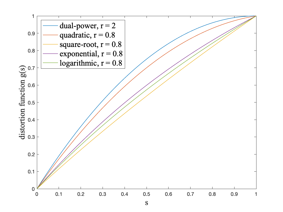
Figure 1: Examples of distortion functions

The limit of the integration in 16, $M_{r}=\frac{r_{\textrm{max}}}{1-\gamma}$ or any problem specific upper bound for $\left\lvert R^{\theta}\right\rvert$. As $g(\cdot)\in[0,1]$, we can infer the following bound on $\rho_{g}(\cdot)$:

$$\left\lvert\rho_{g}(\cdot)\right\rvert\leq 2M_{r}.$$ (17)

The inequality in (17) partially satisfies the conditions specified by (A5) for the DRM.

Recall that the optimization problem in (8) is solved using stochastic gradient algorithm, and for each update iteration, we require estimates of $\rho_{g}(\cdot)$. In the following sections, we describe our algorithms that estimate DRM in on-policy and off-policy RL settings, respectively.

5.1.1 On-policy DRM estimation

We generate $m$ episodes using the policy $\pi_{\theta}$, and estimate the CDF $F_{R^{\theta}}(\cdot)$ using sample averages. We denote by $R^{\theta}_{i}$ the cumulative reward of the episode $i$. We form the estimate $G^{m}_{R^{\theta}}(\cdot)$ of $F_{R^{\theta}}(\cdot)$ as follows:

$$G^{m}_{R^{\theta}}(x)=\frac{1}{m}\sum\limits_{i=1}^{m}\mathds{1}\{R^{\theta}_{i}\leq x\}.$$ (18)

Now, we form an estimate $\hat{\rho}_{g}^{G}(\theta)$ of $\rho_{g}(\theta)$ as follows:

$$\hat{\rho}_{g}^{G}(\theta)\!=\!\!\!\int_{-M_{r}}^{0}\!\!\!\!\!(g(1\!-\!G^{m}_{R^{\theta}}(x))\!-\!1)dx+\!\!\int_{0}^{M_{r}}\!\!\!\!\!g(1\!-\!G^{m}_{R^{\theta}}(x))dx.$$ (19)

Comparing (19) with (16), it is apparent that we have used the empirical distribution function $G^{m}_{R^{\theta}}$ in place of the true CDF $F_{R^{\theta}}$. Similar to $\rho_{g}(\cdot)$, we can infer the following bound on $\hat{\rho}_{g}^{G}(\cdot)$:

$$\left\lvert\hat{\rho}_{g}^{G}(\cdot)\right\rvert\leq 2M_{r}.$$ (20)

The inequality in (20) along with (17) satisfies the conditions specified by (A5) for the DRM in an on-policy RL setting.

We simplify (19) in terms of order statistics as follows:

$$\hat{\rho}_{g}^{G}(\theta)=\sum\limits_{i=1}^{m}{R^{\theta}_{(i)}}\left(g\left(1\!-\!\frac{i\!-\!1}{m}\right)\!-\!g\left(1\!-\!\frac{i}{m}\right)\right),$$ (21)

where $R^{\theta}_{(i)}$ is the $i^{th}$ smallest order statistic of the samples $\{R^{\theta}_{1},\cdots R^{\theta}_{m}\}$. The reader is referred to Lemma 13 in Appendix B for the proof. If we choose the distortion function as the identity function, then the estimator in (21) is merely the sample mean.

We make the following assumptions to ensure the Lipschitzness, and smoothness of the DRM $\rho_{g}$.

(A9).

$\exists M_{g^{\prime}},M_{g^{\prime\prime}}>0:\forall t\in(0,1)$, $\lvert g^{\prime}(t)\rvert\leq M_{g^{\prime}}$, and $\lvert g^{\prime\prime}(t)\rvert\leq M_{g^{\prime\prime}}$.

The assumption (A9) helps us establish that the distortion functions and its derivative are Lipschitz continuous. A few examples of distortion functions, which satisfy (A9) are given in Table 1.

A critical requirement for establishing convergence guarantee is a bound on the MSE of the risk estimation scheme, as given in (A6). The result below shows that this MSE requirement is met by the DRM estimator (19). The proof can be found in Appendix B.

Lemma 1.

Assume (A1)-(A2) and (A9). Then,

$$\mathbb{E}\left[\left\lvert\rho_{g}(\theta)-\hat{\rho}_{g}^{G}(\theta)\right\rvert^{2}\right]\leq\frac{16M_{r}^{2}M_{g^{\prime}}^{2}}{m}.$$

5.1.2 Off-policy DRM estimation

We generate $m$ episodes using the policy $b$ to estimate the CDF $F_{R^{\theta}}(\cdot)$ using importance sampling. We denote by $R^{b}_{i}$ the cumulative reward, and $\psi^{\theta}_{i}$ the importance sampling ratio of the episode $i$. We form the estimate $H^{m}_{R^{\theta}}(\cdot)$ of $F_{R^{\theta}}(\cdot)$ as follows:

$$H^{m}_{R^{\theta}}(x) =\min\{\hat{H}^{m}_{R^{\theta}}(x),1\},\textrm{ where}$$ (22)

$$\hat{H}^{m}_{R^{\theta}}(x) =\frac{1}{m}\sum\limits_{i=1}^{m}\mathds{1}\{R^{b}_{i}\leq x\}\psi^{\theta}_{i}.$$ (23)

In the above, $\hat{H}^{m}_{R^{\theta}}(x)$ is an empirical estimate of $F_{R^{\theta}}(x)$ as $F_{R^{\theta}}(x)=\mathbb{E}\left[\mathds{1}\{R^{b}\leq x\}\psi^{\theta}\right]$. Because of the importance sampling ratio, $\hat{H}^{m}_{R^{\theta}}(x)$ can get a value above $1$. Since we are estimating a CDF, we restrict $\hat{H}^{m}_{R^{\theta}}(x)$ to $H^{m}_{R^{\theta}}(x)$.

Now we form an estimate $\hat{\rho}_{g}^{H}(\theta)$ of $\rho_{g}(\theta)$ as

$$\hat{\rho}_{g}^{H}(\theta)\!=\!\!\!\int\nolimits_{-M_{r}}^{0}\!\!\!\!\!(g(1\!-\!H^{m}_{R^{\theta}}(x))\!-\!1)dx+\!\!\!\int\nolimits_{0}^{M_{r}}\!\!\!\!\!g(1\!-\!H^{m}_{R^{\theta}}(x))dx.$$ (24)

Similar to $\rho_{g}(\cdot)$, we can infer the following bound on $\hat{\rho}_{g}^{H}(\cdot)$:

$$\left\lvert\hat{\rho}_{g}^{H}(\cdot)\right\rvert\leq 2M_{r}.$$ (25)

The inequality in (25) along with (17) satisfies the conditions specified by (A5) for the DRM in an off-policy RL setting.

We can simplify (24) in terms of order statistics as

$$\hat{\rho}_{g}^{H}(\theta) =R^{b}_{(1)}+\sum_{i=2}^{m}{R^{b}_{(i)}}g\left(1\!-\!\min\left\{1,\frac{1}{m}\sum_{k=1}^{i-1}\psi^{\theta}_{(k)}\right\}\right)$$

$$-\sum_{i=1}^{m-1}{R^{b}_{(i)}}g\left(1\!-\!\min\left\{1,\frac{1}{m}\sum_{k=1}^{i}\psi^{\theta}_{(k)}\right\}\right),$$ (26)

where $R^{b}_{(i)}$ is the $i^{th}$ smallest order statistic of the samples $\{R^{b}_{1},\cdots R^{b}_{m}\}$, and $\psi^{\theta}_{(i)}$ is the importance sampling ratio of $R^{b}_{(i)}$. The reader is referred to Lemma 14 in Appendix B for the proof.

A result in the spirit of Lemma 1 for the off-policy setting is given below. The result below shows that the MSE requirement in (A6) is met by the DRM estimator (24). The proof can be found in Appendix B.

Lemma 2.

Assume (A1)-(A4) and (A9). Then,

$$\mathbb{E}\left[\left\lvert\rho_{g}(\theta)-\hat{\rho}_{g}^{H}(\theta)\right\rvert^{2}\right]\leq\frac{16M_{r}^{2}M_{g^{\prime}}^{2}M_{s}^{2}}{m}.$$

5.1.3 Convergence analysis

First we show that the assumptions (A7)-(A8) are satisfied for the DRM using the results from the following lemma (see Appendix B for the proof).

Lemma 3.

$\forall\theta_{1},\theta_{2}\in\mathbb{R}^{d}$,

$$\left\lvert\rho_{g}(\theta_{1})-\rho_{g}(\theta_{2})\right\rvert\leq L_{\rho}\left\lVert\theta_{1}\!-\!\theta_{2}\right\rVert;L_{\rho}=2M_{r}M_{g^{\prime}}M_{e}M_{d},$$

$$\left\lVert\nabla\rho_{g}(\theta_{1})-\nabla\rho_{g}(\theta_{2})\right\rVert\leq L_{\rho^{\prime}}\left\lVert\theta_{1}-\theta_{2}\right\rVert;$$

$$\qquad L_{\rho^{\prime}}=2M_{r}M_{e}\left(M_{h}M_{g^{\prime}}+M_{e}M_{d}^{2}(M_{g^{\prime}}+M_{g^{\prime\prime}})\right).$$

The main result that establishes a non-asymptotic bound for Algorithm 1 with DRM as the risk measure is given below.

Corollary 1.

(DRM-OnP-SF) Assume (A1)-(A2) and (A9). Then, under the conditions of Theorem 1, we have

$$\mathbb{E}\left[\left\lVert\nabla\rho_{g}(\theta_{R})\right\rVert^{2}\right]\leq\frac{2\left(\rho_{g}^{*}-\rho_{g}(\theta_{0})\right)}{\sqrt{N}}+\frac{2d^{2}L_{\rho}^{2}L_{\rho^{\prime}}}{N\sqrt{N}}$$

$$\quad+\frac{4d^{2}L_{\rho}^{2}+d^{2}C_{1}L_{\rho^{\prime}}}{N}+\frac{d^{2}C_{1}+d^{2}L_{\rho^{\prime}}^{2}}{\sqrt{N}}.$$

In the above, $\rho_{g}^{*}\!=\!\max_{\theta\in\mathbb{R}^{d}}\rho_{g}(\theta)$. The constants $C_{1},L_{\rho}$, and $L_{\rho^{\prime}}$ are as in Lemmas 1 and 3, respectively.

Proof.

Lemma 1 implies (A6) holds for DRM estimator. Lemma 3 implies the conditions in (A7) and (A8) hold for DRM. From (17) and (20), we can see that the conditions in (A5) is satisfied for DRM. The main claim now follows by an application of Theorem 1. ∎

For the off-policy case, a non-asymptotic bound can be inferred from Theorem 2 in a similar fashion as the on-policy case, with Lemma 2 in place of Lemma 1, and (25) in place of (20).

Corollary 2.

(DRM-OffP-SF) Assume (A1)-(A9). Then, under the conditions of Theorem 2, we have

$$\mathbb{E}\left[\left\lVert\nabla\rho_{g}(\theta_{R})\right\rVert^{2}\right]\leq\frac{2\left(\rho_{g}^{*}-\rho_{g}(\theta_{0})\right)}{\sqrt{N}}+\frac{2d^{2}L_{\rho}^{2}L_{\rho^{\prime}}}{N\sqrt{N}}$$

$$\quad+\frac{C_{2}4d^{2}L_{\rho}^{2}+d^{2}C_{1}L_{\rho^{\prime}}}{C_{2}N}+\frac{d^{2}C_{1}+C_{2}d^{2}L_{\rho^{\prime}}^{2}}{C_{2}\sqrt{N}}.$$

In the above, $\rho_{g}^{*},L_{\rho}$, and $L_{\rho^{\prime}}$ are as in Corollary 1. The constant $C_{1}$ is as in Lemma 2.

Remark 4.

If we choose the distortion function as the identity function, then the estimator in (16) is merely the sample mean, and we recover the guarantees for a risk-neutral policy gradient algorithm. In particular, our bounds match the guarantees given by Vijayan and Prashanth [2021], which employs an SF-based gradient estimation scheme in a risk-neutral setting, and establishes consistency with the bounds of the REINFORCE style policy gradient algorithm.

5.2 Mean-variance risk measure (MVRM)

The MVRM $\rho_{\lambda}(\theta)$ of $R^{\theta}$, defined in (1), is given by

$$\rho_{\lambda}(\theta)=J(\theta)-\lambda V(\theta),\textrm{ where}$$

$$J(\theta)=\mathbb{E}\left[R^{\theta}\right];\;V(\theta)=\mathbb{E}\left[\left(R^{\theta}\right)^{2}\right]-J(\theta)^{2}.$$ (27)

In the above, $J(\theta)$ is the value function, which is the objective in a risk-neutral RL setting. Further, $V(\theta)$ is the variance of the cumulative reward, and $\lambda$ is a scalar that is used to tradeoff between mean and variance. A popular risk measure in control literature is exponential utility, where the objective is $-\frac{1}{\lambda}\log\mathbb{E}[e^{-\lambda R^{\theta}}]$, with $R^{\theta}$ denoting the cumulative reward. Using a first-order Taylor expansion, it is apparent that

$$-\frac{1}{\lambda}\log\mathbb{E}[e^{-\lambda R^{\theta}}]=\mathbb{E}[R^{\theta}]-\frac{\lambda}{2}\text{Var}[R^{\theta}]+O(\lambda^{2}).$$

Thus, the MVRM risk measure defined above can be seen as an approximation to the exponential utility risk measure. Optimizing the latter risk measure in an RL context is challenging, and to the best of our knowledge, there is no RL algorithm with a compact parameterization for this problem. Instead of using a parameterized family of policies, the authors in Prashanth and Fu [2022] adopt a different approach by treating the policy as a probability vector over all states and actions. Further, they introduce a two timescale tabular algorithm using Q-values within the context of an average-cost MDP setting (see Section 7.1 of Prashanth and Fu [2022] for the details). In contrast, we present a policy gradient algorithm for MVRM with a provable bound on the rate for stationary convergence.

It is easy to see that $\left\lvert J(\theta)\right\rvert\leq M_{r}$ and $V(\theta)\leq M_{r}^{2}$. Hence we could infer the following bound on $\rho_{\lambda}(\cdot)$:

$$\left\lvert\rho_{\lambda}(\cdot)\right\rvert\leq M_{r}(1+\lambda M_{r}).$$ (28)

The inequality in (28) partially satisfies the conditions specified by (A5) for the MVRM.

Next, we describe the estimation of the MVRM in on-policy and off-policy settings, respectively.

5.2.1 On-policy MVRM estimation

We generate $m$ episodes using the policy $\pi_{\theta}$, and estimate $J(\theta)$ and $V(\theta)$ using sample averages. We denote by $R^{\theta}_{i}$ the cumulative reward of the episode $i$. The estimators $\hat{J}_{m}^{\pi}$ of $J(\theta)$ and $\widehat{V}_{m}^{\pi}$ of $V(\theta)$ is defined as follows:

$$\hat{J}_{m}^{\pi}(\theta)=\frac{1}{m}\sum\limits_{i=1}^{m}R^{\theta}_{i};$$ (29)

$$\widehat{V}_{m}^{\pi}(\theta)=\frac{1}{m-1}\sum\limits_{i=1}^{m}\left(R^{\theta}_{i}-\hat{J}_{m}^{\pi}\right)^{2}.$$ (30)

Using Theorem 2-3 in [Mood et al., 1974, chapter V1], we can see that the above estimates are unbiased.

Using (29) and (30), we estimate $\rho_{\lambda}(\theta)$ as follows:

$$\hat{\rho}_{\lambda}^{\pi}(\theta)=\hat{J}_{m}^{\pi}(\theta)-\lambda\widehat{V}_{m}^{\pi}(\theta).$$ (31)

We can see that $\left\lvert\hat{J}_{m}^{\pi}(\cdot)\right\rvert\leq M_{r}$ and $\widehat{V}_{m}^{\pi}(\cdot)\leq 8M_{r}^{2}$. Hence we could infer the following bound on $\hat{\rho}_{\lambda}^{\pi}(\cdot)$:

$$\left\lvert\hat{\rho}_{\lambda}^{\pi}(\cdot)\right\rvert\leq M_{r}(1+8\lambda M_{r}).$$ (32)

The inequality in (32) along with (28) satisfies the conditions specified by (A5) for the MVRM in an on-policy RL setting.

The result below for the mean-variance estimator (31) satisfies an MSE bound of order $O(1/m)$, in turn verify (A6). The proof can be found in Appendix C.

Lemma 4.

Assume (A1)-(A2), and let $m>2$. Then

$$\mathbb{E}\left[\left\lvert\hat{\rho}_{\lambda}^{\pi}(\theta)-\rho_{\lambda}(\theta)\right\rvert^{2}\right]\leq\frac{8M_{r}^{2}+32\lambda^{2}M_{r}^{4}}{m}.$$

5.2.2 Off-policy MVRM estimation

We generate $m$ episodes using the policy $b$ to estimate $J(\theta)$ using importance sampling. We denote by $R^{b}_{i}$ the cumulative reward, and $\psi^{\theta}_{i}$ the importance sampling ratio of the episode $i$. Since $J(\theta)=\mathbb{E}\left[R^{b}\psi^{\theta}\right]$, we estimate it using sample average as follows:

$$\hat{J}_{m}^{b}(\theta)=\frac{1}{m}\sum\limits_{i=1}^{m}R^{b}_{i}\psi^{\theta}_{i};$$ (33)

$$\widehat{V}_{m}^{b}(\theta)=\frac{1}{m-1}\sum\limits_{i=1}^{m}\left(R^{b}_{i}\psi^{\theta}_{i}-\hat{J}_{m}^{b}\right)^{2}.$$ (34)

As in the on-policy setting, these estimates are unbiased.

Now using (33) and (34), we estimate $\rho_{\lambda}(\theta)$ as follows:

$$\hat{\rho}_{\lambda}^{b}(\theta)=\hat{J}_{m}^{b}(\theta)-\lambda\widehat{V}_{m}^{b}(\theta).$$ (35)

Similar to on-policy case, we can see that $\left\lvert\hat{J}_{m}^{b}(\cdot)\right\rvert\leq M_{r}M_{s}$ and $\widehat{V}_{m}^{b}(\cdot)\leq 8M_{r}^{2}M_{s}^{2}$. Hence we could infer the following bound on $\hat{\rho}_{\lambda}^{b}(\cdot)$:

$$\left\lvert\hat{\rho}_{\lambda}^{b}(\cdot)\right\rvert\leq M_{r}M_{s}(1+8\lambda M_{r}M_{s}).$$ (36)

The inequality in (36) along with (28) satisfies the conditions specified by (A5) for the MVRM in an off-policy RL setting.

A result in the spirit of Lemma 4 for the off-policy setting is given below. The result below for the mean-variance estimator (35) satisfies an MSE bound of order $O(1/m)$, in turn verify (A6). The proof can be found in Appendix C.

Lemma 5.

Assume (A1)-(A4), and let $m>2$. Then

$$\mathbb{E}\left[\left\lvert\hat{\rho}_{\lambda}^{b}(\theta)-\rho_{\lambda}(\theta)\right\rvert^{2}\right]\leq\frac{8M_{r}^{2}M_{s}^{2}+32\lambda^{2}M_{r}^{4}M_{s}^{4}}{m}.$$

5.2.3 Convergence analysis

We specialize the result in Proposition 1 to MVRM. Though MVRM is previously analyzed in Tamar et al. [2012], Prashanth and Ghavamzadeh [2013], they only provide asymptotic convergence results. In the following lemma, we show that the assumptions (A7)-(A8) are satisfied for the MVRM. The proof can be found in Appendix C.

Lemma 6.

$\forall\theta_{1},\theta_{2}\in\mathbb{R}^{d}$,

$$\left\lvert\rho_{\lambda}(\theta_{1})-\rho_{\lambda}(\theta_{1})\right\rvert\leq L_{\rho}\left\lVert\theta_{1}-\theta_{2}\right\rVert;$$

$$\qquad L_{\rho}=M_{r}M_{e}M_{d}+3\lambda M_{r}^{2}M_{e}M_{d},\textrm{ and}$$

$$\left\lVert\nabla\rho_{\lambda}(\theta_{1})-\nabla\rho_{\lambda}(\theta_{1})\right\rVert\leq L_{\rho^{\prime}}\left\lVert\theta_{1}-\theta_{2}\right\rVert;$$

$$\qquad L_{\rho^{\prime}}=M_{r}M_{e}\left(M_{h}+M_{e}M_{d}^{2}\right)$$

$$\qquad\qquad+\lambda M_{r}^{2}M_{e}\left(3M_{h}+5M_{e}M_{d}^{2}\right).$$

Corollary 3.

(MVRM-OnP-SF) Assume (A1)-(A2). Let the batch size $m=\sqrt{N}>2$. Then, under the conditions of Theorem 1, we have

$$\mathbb{E}\left[\left\lVert\nabla\rho_{\lambda}(\theta_{R})\right\rVert^{2}\right]\leq\frac{2\left(\rho_{\lambda}^{*}-\rho_{\lambda}(\theta_{0})\right)}{\sqrt{N}}+\frac{2d^{2}L_{\rho}^{2}L_{\rho^{\prime}}}{N\sqrt{N}}$$

$$\quad+\frac{4d^{2}L_{\rho}^{2}+d^{2}C_{1}L_{\rho^{\prime}}}{N}+\frac{d^{2}C_{1}+d^{2}L_{\rho^{\prime}}^{2}}{\sqrt{N}}.$$

In the above, $\rho_{\lambda}^{*}\!=\!\max_{\theta\in\mathbb{R}^{d}}\rho_{\lambda}(\theta)$. The constants $C_{1},L_{\rho}$, and $L_{\rho^{\prime}}$ are as in Lemmas 4 and 6, respectively.

Proof.

Lemma 4 implies (A6) holds for MVRM estimator. Lemma 6 implies the conditions in (A7) and (A8) hold for MVRM. From (28) and (32), we can see that the conditions in (A5) is satisfied for MVRM. The main claim now follows by an application of Theorem 1. ∎

The bound for the off-policy variant follows by using Lemma 5 in place of Lemma 4, and (36) in place of (32).

Corollary 4.

(MVRM-OffP-SF) Assume (A1)-(A4). Let $C_{2}>2$. Then, under the conditions of Theorem 2, we have

$$\mathbb{E}\left[\left\lVert\nabla\rho_{\lambda}(\theta_{R})\right\rVert^{2}\right]\leq\frac{2\left(\rho_{\lambda}^{*}-\rho_{\lambda}(\theta_{0})\right)}{\sqrt{N}}+\frac{2d^{2}L_{\rho}^{2}L_{\rho^{\prime}}}{N\sqrt{N}}$$

$$\quad+\frac{C_{2}4d^{2}L_{\rho}^{2}+d^{2}C_{1}L_{\rho^{\prime}}}{C_{2}N}+\frac{d^{2}C_{1}+C_{2}d^{2}L_{\rho^{\prime}}^{2}}{C_{2}\sqrt{N}}.$$

In the above, $\rho_{\lambda}^{*},L_{\rho}$, and $L_{\rho^{\prime}}$ are as in Corollary 3. The constant $C_{1}$ is as in Lemma 5.

6 Conclusions

We proposed two policy gradient algorithms that cater to the broad class of smooth risk measures. Both algorithms employed an SF-based gradient estimation scheme, and were shown to work in on-policy as well as off-policy RL settings. We derived non-asymptotic bounds that quantify the rate of convergence to our proposed algorithms to a stationary point of the smooth risk measure. As special cases, we showed that our theory and algorithms apply to optimization of MVRM and DRM, respectively. To the best of our knowledge, policy gradient algorithms with non-asymptotic convergence guarantees are not available in the literature for smooth risk measures in general, and the special cases of DRM and MVRM, in particular.

As future work, it would be interesting to investigate the convergence properties of non-smooth risk measures such as CVaR and CPT. While CVaR can be expressed as a DRM, its distortion function is not smooth, and CPT has a similar distortion function that is also non-smooth. To develop policy gradient algorithms, one could explore the possibility of using smooth approximations of these distortion functions and analyze their convergence properties.

Appendix A Results for the policy gradient template

A.1 Results with true objective function $\rho(\cdot)$

The following lemmas establish some results related to the SF-based gradient estimate.

Lemma 7.

$\mathbb{E}\left[\widehat{\nabla}_{\mu,n}\rho(\theta)\mid\theta\right]=\nabla\rho_{\mu}(\theta)$.

Proof.

We follow the technique from Shamir [2017]. Since $v_{1:n}$ are i.i.d r.v.s, and have symmetric distribution around the origin, we obtain

$$\mathbb{E}\left[\widehat{\nabla}_{\mu,n}\rho(\theta)\mid\theta\right] =\mathbb{E}_{v_{1:n}}\left[\widehat{\nabla}_{\mu,n}\rho(\theta)\right]=\frac{d}{2\mu n}\sum_{i=1}^{n}\mathbb{E}_{v}\left[\left(\rho({\theta+\mu v})-\rho({\theta-\mu v})\right)v\right]$$

$$=\frac{d}{2\mu}\left(\mathbb{E}_{v}\left[\rho({\theta+\mu v})v\right]+\mathbb{E}_{v}\left[\rho({\theta+\mu(-v)})(-v)\right]\right)=\frac{d}{\mu}\mathbb{E}_{v}\left[\rho({\theta+\mu v})v\right]=\nabla\rho_{\mu}(\theta),$$

where last equality follows from [Flaxman et al., 2005, Lemma 2.1]. ∎

Lemma 8.

Suppose $\forall\theta_{1},\theta_{2}\in\mathbb{R}^{d}$, $\left\lVert\nabla\rho(\theta_{1})-\nabla\rho(\theta_{2})\right\rVert\leq L_{\rho^{\prime}}\left\lVert\theta_{1}-\theta_{2}\right\rVert$. Then $\left\lVert\nabla\rho_{\mu}(\theta)-\nabla\rho(\theta)\right\rVert\leq\frac{\mu dL_{\rho^{\prime}}}{2}$.

Proof.

The result follows from [Gao et al., 2018, Proposition 7.5]. ∎

Lemma 9.

Suppose $\forall\theta\in\mathbb{R}^{d}$, $\rho(\theta)$ is bounded and $\forall\theta_{1},\theta_{2}\in\mathbb{R}^{d}$, $\left\lvert\rho(\theta_{1})-\rho(\theta_{2})\right\rvert\leq L_{\rho}\left\lVert\theta_{1}-\theta_{2}\right\rVert$. Then $\mathbb{E}\left[\left\lVert\widehat{\nabla}_{\mu,n}\rho(\theta)\right\rVert^{2}\right]\leq\frac{d^{2}L_{\rho}^{2}}{n}$.

Proof.

Since $\forall v\in\mathbb{S}^{d-1},\;\lVert v\rVert=1$, from (12), we have

$$\mathbb{E}_{v_{1:n}}\left[\left\lVert\widehat{\nabla}_{\mu,n}\rho(\theta)\right\rVert^{2}\right] \stackrel{{\scriptstyle(a)}}{{\leq}}\frac{d^{2}}{4\mu^{2}n^{2}}\sum_{i=1}^{n}\mathbb{E}_{v}\left[\left\lVert\left(\rho({\theta+\mu v})-\rho({\theta-\mu v})\right)v\right\rVert^{2}\right]$$

$$\leq\frac{d^{2}}{4\mu^{2}n}\mathbb{E}_{v}\left[\left\lVert\left(\rho({\theta+\mu v})-\rho({\theta-\mu v})\right)\right\rVert^{2}\lVert v\rVert^{2}\right]$$

$$\leq\frac{d^{2}L_{\rho}^{2}}{n}\left\lVert v\right\rVert^{4}=\frac{d^{2}L_{\rho}^{2}}{n},$$

where $(a)$ follows from the fact that $v_{1:n}$ are i.i.d mean zero r.v.s, and $\rho(\cdot)$ is bounded. Finally,

$$\mathbb{E}\left[\left\lVert\widehat{\nabla}_{\mu,n}\rho(\theta)\right\rVert^{2}\right]=\mathbb{E}\left[\mathbb{E}_{v_{1:n}}\left[\left\lVert\widehat{\nabla}_{\mu,n}\rho(\theta)\right\rVert^{2}\right]\right]\leq\frac{d^{2}L_{\rho}^{2}}{n}.$$

∎

A.2 Results with approximate objective function $\hat{\rho}_{m}(\cdot)$

The following lemmas establish bounds for the bias and variance of the gradient estimate in (13).

Lemma 10.

Suppose $\forall\theta\in\mathbb{R}^{d}$, $\rho(\theta)$ and $\hat{\rho}_{m}(\theta)$ are bounded, and $\mathbb{E}\left[\left\lvert\rho(\theta)-\hat{\rho}_{m}(\theta)\right\rvert^{2}\right]\leq\frac{C_{1}}{m}$. Then

$$\mathbb{E}\left[\left\lVert\frac{d}{n}\sum\limits_{i=1}^{n}\frac{\hat{\rho}_{m}({\theta\pm\mu v_{i}})-\rho({\theta\pm\mu v_{i}})}{2\mu}v_{i}\right\rVert^{2}\right]\leq\frac{d^{2}C_{1}}{4\mu^{2}mn}.$$

Proof.

Notice that

$$\mathbb{E}\left[\left\lVert\frac{d}{n}\sum_{i=1}^{n}\frac{\hat{\rho}_{m}({\theta\pm\mu v_{i}})-\rho({\theta\pm\mu v_{i}})}{2\mu}v_{i}\right\rVert^{2}\right]\leq\frac{d^{2}}{4n^{2}\mu^{2}}\mathbb{E}\left[\mathbb{E}_{v_{1:n}}\left\lVert\sum_{i=1}^{n}\left(\hat{\rho}_{m}({\theta\pm\mu v_{i}})-\rho({\theta\pm\mu v_{i}})\right)v_{i}\right\rVert^{2}\right]$$

$$\stackrel{{\scriptstyle(a)}}{{\leq}}\frac{d^{2}n}{4\mu^{2}n^{2}}\mathbb{E}\left[\mathbb{E}_{v}\left[\left\lVert\hat{\rho}_{m}({\theta\pm\mu v})-\rho({\theta\pm\mu v})v\right\rVert^{2}\right]\right]$$

$$\stackrel{{\scriptstyle(b)}}{{\leq}}\frac{d^{2}}{4\mu^{2}n}\mathbb{E}\left[\mathbb{E}_{v}\left[\left(\hat{\rho}_{m}({\theta\pm\mu v})-\rho({\theta\pm\mu v})\right)^{2}\right]\right]$$

$$=\frac{d^{2}}{4\mu^{2}n}\mathbb{E}\left[\left(\hat{\rho}_{m}({\theta\pm\mu v})-\rho({\theta\pm\mu v})\right)^{2}\right]\leq\frac{d^{2}C_{1}}{4\mu^{2}mn},$$

where $(a)$ follows from the fact that $v_{1:n}$ are i.i.d mean zero r.v.s, and $\hat{\rho}_{m}(\cdot)$ and $\rho(\cdot)$ are bounded, and $(b)$ follows since $\lVert v\rVert=1$. ∎

Lemma 11.

$\mathbb{E}\left[\left\lVert\widehat{\nabla}_{\mu,n}\hat{\rho}_{m}({\theta})-\nabla\rho(\theta)\right\rVert^{2}\right]\leq\frac{4d^{2}L_{\rho}^{2}}{n}+\mu^{2}d^{2}L_{\rho^{\prime}}^{2}+\frac{d^{2}C_{1}}{\mu^{2}mn}$

Proof.

Notice that

$$\widehat{\nabla}_{\mu,n}\hat{\rho}_{m}({\theta})=\frac{d}{n}\sum_{i=1}^{n}\frac{\hat{\rho}_{m}({\theta+\mu v_{i}})-\hat{\rho}_{m}({\theta-\mu v_{i}})}{2\mu}v_{i}$$

$$=\frac{d}{n}\sum_{i=1}^{n}\frac{\rho({\theta+\mu v_{i}})-\rho({\theta-\mu v_{i}})}{2\mu}v_{i}+\frac{d}{n}\sum_{i=1}^{n}\frac{\hat{\rho}_{m}({\theta+\mu v_{i}})-\rho({\theta+\mu v_{i}})}{2\mu}v_{i}+\frac{d}{n}\sum_{i=1}^{n}\frac{\rho({\theta-\mu v_{i}})-\hat{\rho}_{m}({\theta-\mu v_{i}})}{2\mu}v_{i}$$

$$=\widehat{\nabla}_{\mu,n}\rho({\theta})+\frac{d}{n}\sum_{i=1}^{n}\frac{\hat{\rho}_{m}({\theta+\mu v_{i}})-\rho({\theta+\mu v_{i}})}{2\mu}v_{i}+\frac{d}{n}\sum_{i=1}^{n}\frac{\rho({\theta-\mu v_{i}})-\hat{\rho}_{m}({\theta-\mu v_{i}})}{2\mu}v_{i}.$$ (37)

From (37) and Lemma 10, we obtain

$$\mathbb{E}\left[\left\lVert\widehat{\nabla}_{\mu,n}\hat{\rho}_{m}({\theta})-\nabla\rho(\theta)\right\rVert^{2}\right]\leq 2\mathbb{E}\left[\left\lVert\widehat{\nabla}_{\mu,n}\rho({\theta})-\nabla\rho_{g}(\theta)\right\rVert^{2}\right]+\frac{d^{2}C_{1}}{\mu^{2}mn}$$

$$\stackrel{{\scriptstyle(a)}}{{\leq}}4\mathbb{E}\left[\left\lVert\widehat{\nabla}_{\mu,n}\rho({\theta})-\mathbb{E}\left[\widehat{\nabla}_{\mu,n}\rho(\theta)\mid\theta\right]\right\rVert^{2}\right]+4\mathbb{E}\left[\left\lVert\nabla\rho_{\mu}(\theta)-\nabla\rho(\theta)\right\rVert^{2}\right]+\frac{d^{2}C_{1}}{\mu^{2}mn}$$

$$\stackrel{{\scriptstyle(b)}}{{\leq}}4\mathbb{E}\left[\left\lVert\widehat{\nabla}_{\mu,n}\rho_{g}({\theta})\right\rVert^{2}\right]+\mu^{2}d^{2}L_{\rho^{\prime}}^{2}+\frac{d^{2}C_{1}}{\mu^{2}mn}$$

$$\stackrel{{\scriptstyle(c)}}{{\leq}}\frac{4d^{2}L_{\rho}^{2}}{n}+\mu^{2}d^{2}L_{\rho^{\prime}}^{2}+\frac{d^{2}C_{1}}{\mu^{2}mn},$$

where $(a)$ follows from Lemma 7, $(b)$ follows from Lemma 8 and since $\mathbb{E}[\lVert X-E[X\mid Y]\rVert^{2}]\leq\mathbb{E}[\lVert X\rVert^{2}]$, and $(c)$ follows from Lemma 9. ∎

Lemma 12.

$\mathbb{E}\left[\left\lVert\widehat{\nabla}_{\mu,n}\hat{\rho}_{m}({\theta})\right\rVert^{2}\right]\leq\frac{2d^{2}L_{\rho}^{2}}{n}+\frac{d^{2}C_{1}}{\mu^{2}mn}$.

Proof.

Using (37) and Lemma 10, we obtain

$$\mathbb{E}\left[\left\lVert\widehat{\nabla}_{\mu,n}\hat{\rho}_{m}({\theta})\right\rVert^{2}\right] \leq 2\mathbb{E}\left[\left\lVert\widehat{\nabla}_{\mu,n}\rho({\theta})\right\rVert^{2}\right]+\frac{d^{2}C_{1}}{\mu^{2}mn}\leq\frac{2d^{2}L_{\rho}^{2}}{n}+\frac{d^{2}C_{1}}{\mu^{2}mn},$$

where the last inequality follows from Lemma 9. ∎

A.3 Proof of Proposition 1

Using the fundamental theorem of calculus, we obtain

$$\rho(\theta_{k})-\rho(\theta_{k+1})=\langle\nabla\rho(\theta_{k}),\theta_{k}-\theta_{k+1}\rangle+\int_{0}^{1}\left\langle\nabla\rho(\theta_{k+1}+\tau(\theta_{k}-\theta_{k+1}))-\nabla\rho(\theta_{k}),\theta_{k}-\theta_{k+1}\right\rangle d\tau$$

$$\leq\langle\nabla\rho(\theta_{k}),\theta_{k}-\theta_{k+1}\rangle+\int_{0}^{1}\left\lVert\nabla\rho(\theta_{k+1}+\tau(\theta_{k}-\theta_{k+1}))-\nabla\rho(\theta_{k})\right\rVert\left\lVert\theta_{k}-\theta_{k+1}\right\rVert d\tau$$

$$\stackrel{{\scriptstyle(a)}}{{\leq}}\left\langle\nabla\rho(\theta_{k}),\theta_{k}-\theta_{k+1}\right\rangle+L_{\rho^{\prime}}\left\lVert\theta_{k}-\theta_{k+1}\right\rVert^{2}\int_{0}^{1}(1-\tau)d\tau$$

$$=\left\langle\nabla\rho(\theta_{k}),\theta_{k}-\theta_{k+1}\right\rangle+\frac{L_{\rho^{\prime}}}{2}\left\lVert\theta_{k}-\theta_{k+1}\right\rVert^{2}$$

$$=\alpha\left\langle\nabla\rho(\theta_{k}),-\widehat{\nabla}_{\mu,n}\hat{\rho}_{m}(\theta_{k})\right\rangle+\frac{L_{\rho^{\prime}}}{2}\alpha^{2}\left\lVert\widehat{\nabla}_{\mu,n}\hat{\rho}_{m}(\theta_{k})\right\rVert^{2}$$

$$=\alpha\left\langle\nabla\rho(\theta_{k}),\nabla\rho(\theta_{k})-\widehat{\nabla}_{\mu,n}\hat{\rho}_{m}(\theta_{k})\right\rangle-\alpha\left\lVert\nabla\rho(\theta_{k})\right\rVert^{2}+\frac{L_{\rho^{\prime}}}{2}\alpha^{2}\left\lVert\widehat{\nabla}_{\mu,n}\hat{\rho}_{m}(\theta_{k})\right\rVert^{2}$$

$$\stackrel{{\scriptstyle(b)}}{{\leq}}\frac{\alpha}{2}\left\lVert\nabla\rho(\theta_{k})\right\rVert^{2}+\frac{\alpha}{2}\left\lVert\nabla\rho(\theta_{k})-\widehat{\nabla}_{\mu,n}\hat{\rho}_{m}(\theta_{k})\right\rVert^{2}-\alpha\left\lVert\nabla\rho(\theta_{k})\right\rVert^{2}+\frac{L_{\rho^{\prime}}}{2}\alpha^{2}\left\lVert\widehat{\nabla}_{\mu,n}\hat{\rho}_{m}(\theta_{k})\right\rVert^{2}$$

$$=\frac{\alpha}{2}\left\lVert\nabla\rho(\theta_{k})-\widehat{\nabla}_{\mu,n}\hat{\rho}_{m}(\theta_{k})\right\rVert^{2}-\frac{\alpha}{2}\left\lVert\nabla\rho(\theta_{k})\right\rVert^{2}+\frac{L_{\rho^{\prime}}}{2}\alpha^{2}\left\lVert\widehat{\nabla}_{\mu,n}\hat{\rho}_{m}(\theta_{k})\right\rVert^{2}.$$ (38)

In the above the step $(a)$ follows since $\rho(\cdot)$ is smooth and the step $(b)$ follows from $2\langle a,b\rangle\leq\lVert a\rVert^{2}+\|b\rVert^{2}$. Rearranging and taking expectations on both sides of (38), we obtain

$$\alpha\mathbb{E}\left[\left\lVert\nabla\rho(\theta_{k})\right\rVert^{2}\right]$$

$$\leq 2\mathbb{E}\left[\rho(\theta_{k+1})-\rho(\theta_{k})\right]+L_{\rho^{\prime}}\alpha^{2}\mathbb{E}\left[\left\lVert\widehat{\nabla}_{\mu,n}\hat{\rho}_{m}(\theta_{k})\right\rVert^{2}\right]+\alpha\mathbb{E}\left[\left\lVert\nabla\rho(\theta_{k})-\widehat{\nabla}_{\mu,n}\hat{\rho}_{m}(\theta_{k})\right\rVert^{2}\right]$$

$$\leq 2\mathbb{E}\left[\rho(\theta_{k+1})-\rho(\theta_{k})\right]+L_{\rho^{\prime}}\alpha^{2}\left(\frac{2d^{2}L_{\rho}^{2}}{n}+\frac{d^{2}C_{1}}{\mu^{2}mn}\right)+\alpha\left(\frac{4d^{2}L_{\rho}^{2}}{n}+\mu^{2}d^{2}L_{\rho^{\prime}}^{2}+\frac{d^{2}C_{1}}{\mu^{2}mn}\right)$$ (39)

where the last inequality follows from lemmas 11-12.

Summing up (39) from $k=0,\cdots,N-1$, we obtain

$$\alpha\sum\limits_{k=0}^{N-1}\mathbb{E}\left[\left\lVert\nabla\rho(\theta_{k})\right\rVert^{2}\right]\leq 2\mathbb{E}\left[\rho(\theta_{N})-\rho(\theta_{0})\right]+NL_{\rho^{\prime}}\alpha^{2}\left(\frac{2d^{2}L_{\rho}^{2}}{n}+\frac{d^{2}C_{1}}{\mu^{2}mn}\right)+N\alpha\left(\frac{4d^{2}L_{\rho}^{2}}{n}+\mu^{2}d^{2}L_{\rho^{\prime}}^{2}+\frac{d^{2}C_{1}}{\mu^{2}mn}\right).$$

Since $\theta_{R}$ is chosen uniformly at random from the policy iterates $\{\theta_{0},\cdots,\theta_{N-1}\}$, we obtain

$$\mathbb{E}\left[\left\lVert\nabla\rho(\theta_{R})\right\rVert^{2}\right] =\frac{1}{N}\sum\limits_{k=0}^{N-1}\mathbb{E}\left[\left\lVert\nabla\rho(\theta_{k})\right\rVert^{2}\right]$$

$$\leq\frac{2\left(\rho^{*}-\rho(\theta_{0})\right)}{N\alpha}+L_{\rho^{\prime}}\alpha\left(\frac{2d^{2}L_{\rho}^{2}}{n}+\frac{d^{2}C_{1}}{\mu^{2}mn}\right)+\frac{4d^{2}L_{\rho}^{2}}{n}+\mu^{2}d^{2}L_{\rho^{\prime}}^{2}+\frac{d^{2}C_{1}}{\mu^{2}mn}.$$

∎

Appendix B DRM

B.1 Estimating DRM using Order statistics

The following lemma estimates the DRM in an on-policy RL setting.

Lemma 13.

$\hat{\rho}_{g}^{G}(\theta)=\sum\limits_{i=1}^{m}{R^{\theta}_{(i)}}\left(g\left(1-\frac{i-1}{m}\right)-g\left(1-\frac{i}{m}\right)\right)$.

Proof.

Our proof follows the technique from Kim [2010]. We rewrite (18) as

$$G^{m}_{R^{\theta}}(x)=\begin{cases}0,&\textrm{if }x<R^{\theta}_{(1)}\\ \frac{i}{m},&\textrm{if }R^{\theta}_{(i)}\leq x<R^{\theta}_{(i+1)},i\in\{1,\!\cdots\!,m-1\}\\ 1,&\textrm{if }x\geq R^{\theta}_{(m)},\\ \end{cases}$$ (40)

where $R^{\theta}_{(i)}$ is the $i^{th}$ smallest order statistic from the samples $R^{\theta}_{1},\cdots R^{\theta}_{m}$.

We assume without loss of generality that $R^{\theta}_{(j)}<0<R^{\theta}_{(j+1)}$, and obtain,

$$\hat{\rho}_{g}^{G}(\theta)=\int\limits_{-M_{r}}^{0}(g(1-G^{m}_{R^{\theta}}(x))-1)dx+\int\limits_{0}^{M_{r}}g(1-G^{m}_{R^{\theta}}(x))dx$$

$$=\int\limits_{-M_{r}}^{R^{\theta}_{(1)}}(g(1-G^{m}_{R^{\theta}}(x))-1)dx+\sum_{i=2}^{j}\int\limits_{R^{\theta}_{(i-1)}}^{R^{\theta}_{(i)}}(g(1-G^{m}_{R^{\theta}}(x))-1)dx+\int\limits_{R^{\theta}_{(j)}}^{0}(g(1-G^{m}_{R^{\theta}}(x))-1)dx$$

$$\quad+\int\limits_{0}^{R^{\theta}_{(j+1)}}g(1-G^{m}_{R^{\theta}}(x))dx+\sum_{i=j+1}^{m-1}\int\limits_{R^{\theta}_{(i)}}^{R^{\theta}_{(i+1)}}g(1-G^{m}_{R^{\theta}}(x))dx+\int\limits_{R^{\theta}_{(m)}}^{M_{r}}g(1-G^{m}_{R^{\theta}}(x))dx$$

$$=\sum_{i=2}^{j}\int\limits_{R^{\theta}_{(i-1)}}^{R^{\theta}_{(i)}}\left(g\left(1-\frac{i-1}{m}\right)-1\right)dx+\int\limits_{R^{\theta}_{(j)}}^{0}\left(g\left(1-\frac{j}{m}\right)-1\right)dx+\int\limits_{0}^{R^{\theta}_{(j+1)}}g\left(1-\frac{j}{m}\right)dx$$

$$\quad+\sum_{i=j+1}^{m-1}\int\limits_{R^{\theta}_{(i)}}^{R^{\theta}_{(i+1)}}g\left(1-\frac{i}{m}\right)dx$$

$$=\sum_{i=2}^{j}\left({R^{\theta}_{(i)}}-{R^{\theta}_{(i-1)}}\right)\left(g\left(1-\frac{i-1}{m}\right)-1\right)-{R^{\theta}_{(j)}}\left(g\left(1-\frac{j}{m}\right)-1\right)+{R^{\theta}_{(j+1)}}g\left(1-\frac{j}{m}\right)$$

$$\quad+\sum_{i=j+1}^{m-1}\left({R^{\theta}_{(i+1)}}-{R^{\theta}_{(i)}}\right)g\left(1\!-\!\frac{i}{m}\right)$$

$$=\sum_{i=2}^{j}\left({R^{\theta}_{(i)}}-{R^{\theta}_{(i-1)}}\right)g\left(1-\frac{i-1}{m}\right)+{R^{\theta}_{(1)}}+\sum_{i=j}^{m-1}\left({R^{\theta}_{(i+1)}}-{R^{\theta}_{(i)}}\right)g\left(1-\frac{i}{m}\right)$$

$$=\sum_{i=1}^{m}{R^{\theta}_{(i)}}g\left(1-\frac{i-1}{m}\right)-\sum_{i=1}^{m-1}{R^{\theta}_{(i)}}g\left(1-\frac{i}{m}\right)$$

$$=\sum_{i=1}^{m}{R^{\theta}_{(i)}}\left(g\left(1-\frac{i-1}{m}\right)-g\left(1-\frac{i}{m}\right)\right).$$

∎

The following lemma estimates the DRM in an off-policy RL setting.

Lemma 14.

$\hat{\rho}_{g}^{H}(\theta)=R^{b}_{(1)}+\sum\limits_{i=2}^{m}{R^{b}_{(i)}}g\left(1-\min\left\{1,\frac{1}{m}\sum\limits_{k=1}^{i-1}\psi^{\theta}_{(k)}\right\}\right)-\sum\limits_{i=1}^{m-1}{R^{b}_{(i)}}g\left(1-\min\left\{1,\frac{1}{m}\sum\limits_{k=1}^{i}\psi^{\theta}_{(k)}\right\}\right)$.

Proof.

We rewrite (22) as

$$H^{m}_{R^{\theta}}(x)=\begin{cases}0,&\textrm{if }x<R^{b}_{(1)}\\ min\{1,\frac{1}{m}\sum\limits_{j=1}^{i}\psi^{\theta}_{(j)}\},&\textrm{if }R^{b}_{(i)}\leq x<R^{\theta}_{(i+1)},i\in\{1,\!\cdots\!,m-1\}\\ 1,&\textrm{if }x\geq R^{b}_{(m)},\\ \end{cases}$$ (41)

where $R^{b}_{(i)}$ is the $i^{th}$ smallest order statistic from the samples $R^{b}_{1},\cdots R^{b}_{m}$, and $\psi^{\theta}_{(i)}$ is the importance sampling ratio of $R^{b}_{(i)}$.

We assume without loss of generality that $R^{b}_{(j)}<0<R^{b}_{(j+1)}$, and obtain,

$$\hat{\rho}_{g}^{H}(\theta)=\int\limits_{-M_{r}}^{0}(g(1-H^{m}_{R^{\theta}}(x))-1)dx+\int\limits_{0}^{M_{r}}g(1-H^{m}_{R^{\theta}}(x))dx$$

$$=\int\limits_{-M_{r}}^{R^{b}_{(1)}}(g(1-H^{m}_{R^{\theta}}(x))-1)dx+\sum_{i=2}^{j}\int\limits_{R^{b}_{(i-1)}}^{R^{b}_{(i)}}(g(1-H^{m}_{R^{\theta}}(x))-1)dx+\int\limits_{R^{b}_{(j)}}^{0}(g(1-H^{m}_{R^{\theta}}(x))-1)dx$$

$$\quad+\int\limits_{0}^{R^{b}_{(j+1)}}g(1-H^{m}_{R^{\theta}}(x))dx+\sum_{i=j+1}^{m-1}\int\limits_{R^{b}_{(i)}}^{R^{b}_{(i+1)}}g(1-H^{m}_{R^{\theta}}(x))dx+\int\limits_{R^{b}_{(m)}}^{M_{r}}g(1-H^{m}_{R^{\theta}}(x))dx$$

$$=\sum_{i=2}^{j}\int\limits_{R^{b}_{(i-1)}}^{R^{b}_{(i)}}\left(g\left(1-min\left\{1,\frac{1}{m}\sum_{k=1}^{i-1}\psi^{\theta}_{(k)}\right\}\right)-1\right)dx+\int\limits_{R^{b}_{(j)}}^{0}\left(g\left(1-min\left\{1,\frac{1}{m}\sum_{k=1}^{j}\psi^{\theta}_{(k)}\right\}\right)-1\right)dx$$

$$\quad+\int\limits_{0}^{R^{b}_{(j+1)}}g\left(1-\min\left\{1,\frac{1}{m}\sum_{k=1}^{j}\psi^{\theta}_{(k)}\right\}\right)dx+\sum_{i=j+1}^{m-1}\int\limits_{R^{b}_{(i)}}^{R^{b}_{(i+1)}}g\left(1-\min\left\{1,\frac{1}{m}\sum_{k=1}^{i}\psi^{\theta}_{(k)}\right\}\right)dx$$

$$=\sum_{i=2}^{j}\left({R^{b}_{(i)}}-{R^{b}_{(i-1)}}\right)\left(g\left(1-\min\left\{1,\frac{1}{m}\sum_{k=1}^{i-1}\psi^{\theta}_{(k)}\right\}\right)-1\right)-{R^{b}_{(j)}}\left(g\left(1-\min\left\{1,\frac{1}{m}\sum_{k=1}^{j}\psi^{\theta}_{(k)}\right\}\right)-1\right)$$

$$\quad+{R^{b}_{(j+1)}}g\left(1-\min\left\{1,\frac{1}{m}\sum_{k=1}^{j}\psi^{\theta}_{(k)}\right\}\right)+\sum_{i=j+1}^{m-1}\left({R^{b}_{(i+1)}}-{R^{b}_{(i)}}\right)g\left(1-\min\left\{1,\frac{1}{m}\sum_{k=1}^{i}\psi^{\theta}_{(k)}\right\}\right)$$

$$=\sum_{i=2}^{j}\left({R^{b}_{(i)}}-{R^{b}_{(i-1)}}\right)g\left(1-\min\left\{1,\frac{1}{m}\sum_{k=1}^{i-1}\psi^{\theta}_{(k)}\right\}\right)+{R^{b}_{(1)}}$$

$$\quad+\sum_{i=j}^{m-1}\left({R^{b}_{(i+1)}}-{R^{b}_{(i)}}\right)g\left(1-\min\left\{1,\frac{1}{m}\sum_{k=1}^{i}\psi^{\theta}_{(k)}\right\}\right)$$

$$=R^{b}_{(1)}+\sum_{i=2}^{m}{R^{b}_{(i)}}g\left(1-\min\left\{1,\frac{1}{m}\sum_{k=1}^{i-1}\psi^{\theta}_{(k)}\right\}\right)-\sum_{i=1}^{m-1}{R^{b}_{(i)}}g\left(1-\min\left\{1,\frac{1}{m}\sum_{k=1}^{i}\psi^{\theta}_{(k)}\right\}\right).$$

∎

B.2 The estimation error of the DRM

In the following lemma, we bound the estimation error of the DRM in an on-policy RL setting.

Proof.

(Lemma 1) Since $\forall x\in(-M_{r},M_{r}),\left\lvert\mathds{1}\{R^{\theta}\leq x\}\right\rvert\leq 1$ a.s., using Hoeffding’s inequality, we obtain $\forall x\in(-M_{r},M_{r})$,

$$\mathbb{P}\left(\left\lvert G^{m}_{R^{\theta}}(x)-F_{R^{\theta}}(x)\right\rvert>\epsilon\right)\leq 2\exp\left(-\frac{m\epsilon^{2}}{2}\right),\textrm{ and}$$

$$\mathbb{E}\left[\left\lvert G^{m}_{R^{\theta}}(x)-F_{R^{\theta}}(x)\right\rvert^{2}\right]=\int_{0}^{\infty}\mathbb{P}\left(\left\lvert G^{m}_{R^{\theta}}(x)-F_{R^{\theta}}(x)\right\rvert>\sqrt{\epsilon}\right)d\epsilon\leq\int_{0}^{\infty}2\exp\left(-\frac{m\epsilon}{2}\right)d\epsilon=\frac{4}{m}.$$ (42)

Now,

$$\mathbb{E}\left[\left\lvert\rho_{g}(\theta)-\hat{\rho}_{g}^{G}(\theta)\right\rvert^{2}\right]=\mathbb{E}\left[\left\lvert\int_{-M_{r}}^{M_{r}}(g(1-F_{R^{\theta}}(x))-g(1-G^{m}_{R^{\theta}}(x)))dx\right\rvert^{2}\right]$$

$$\stackrel{{\scriptstyle(a)}}{{\leq}}2M_{r}\mathbb{E}\left[\int_{-M_{r}}^{M_{r}}\left\lvert(g(1-F_{R^{\theta}}(x))-g(1-G^{m}_{R^{\theta}}(x)))\right\rvert^{2}dx\right]$$

$$\stackrel{{\scriptstyle(b)}}{{\leq}}2M_{r}\int_{-M_{r}}^{M_{r}}\mathbb{E}\left[\left\lvert(g(1-F_{R^{\theta}}(x))-g(1-G^{m}_{R^{\theta}}(x)))\right\rvert^{2}\right]dx$$

$$\stackrel{{\scriptstyle(c)}}{{\leq}}2M_{r}M_{g^{\prime}}^{2}\!\int_{-M_{r}}^{M_{r}}\mathbb{E}\left[\left\lvert G^{m}_{R^{\theta}}(x)-F_{R^{\theta}}(x)\right\rvert^{2}\right]dx$$

$$\stackrel{{\scriptstyle(d)}}{{\leq}}2M_{r}M_{g^{\prime}}^{2}\int_{-M_{r}}^{M_{r}}\frac{4}{m}dx=\frac{16M_{r}^{2}M_{g^{\prime}}^{2}}{m},$$ (43)

where $(a)$ follows from the Cauchy-Schwarz inequality, $(b)$ follows from the Fubini’s theorem, $(c)$ follows from Lemma 15, and $(d)$ follows from (42). ∎

In the following lemma, we bound the estimation error of the DRM in an off-policy RL setting.

Proof.

(Lemma 2) We use parallel arguments to the proof of Lemma 1.

From (6), we obtain $\forall x\in(-M_{r},M_{r})$, $\left\lvert\mathds{1}\{R^{\theta}\leq x\}\psi^{\theta}\right\rvert\leq M_{s}$ a.s. From Hoeffding inequality, we obtain $\forall x\in(-M_{r},M_{r})$,

$$\mathbb{P}\left(\left\lvert\hat{H}^{m}_{R^{\theta}}(x)-F_{R^{\theta}}(x)\right\rvert>\epsilon\right)\leq 2\exp\left(-\frac{m\epsilon^{2}}{2M_{s}^{2}}\right).$$ (44)

From (22) and (23), we observe that $\mathbb{P}\left(\left\lvert H^{m}_{R^{\theta}}(x)-F_{R^{\theta}}(x)\right\rvert>\epsilon\right)\leq\mathbb{P}\left(\left\lvert\hat{H}^{m}_{R^{\theta}}(x)-F_{R^{\theta}}(x)\right\rvert>\epsilon\right)$. Hence, we obtain $\forall x\in(-M_{r},M_{r})$,

$$\mathbb{P}\left(\left\lvert H^{m}_{R^{\theta}}(x)-F_{R^{\theta}}(x)\right\rvert>\epsilon\right)\leq 2\exp\left(-\frac{m\epsilon^{2}}{2M_{s}^{2}}\right).$$ (45)

Using similar arguments as in (42) along with (45), we obtain $\forall x\in[-M_{r},M_{r}]$,

$$\mathbb{E}\left[\left\lvert H^{m}_{R^{\theta}}(x)-F_{R^{\theta}}(x)\right\rvert^{2}\right]\leq\frac{4M_{s}^{2}}{m},\forall x.$$ (46)

Using similar arguments as in (43) along with (46), we obtain

$$\mathbb{E}\left[\left\lvert\rho_{g}(\theta)-\hat{\rho}_{g}^{H}(\theta)\right\rvert^{2}\right]=\frac{16M_{r}^{2}M_{g^{\prime}}^{2}M_{s}^{2}}{m}.$$

∎

B.3 Lipschitz properties of the DRM and its gradient

B.3.1 Results related to the distortion function

The following lemma establishes Lipschitzness of the $g(\cdot)$, and $g^{\prime}(\cdot)$. We require this result to establish the smoothness of the DRM.

Lemma 15.

$\forall t,t^{\prime}\in(0,1)$,$\left\lvert g(t)-g(t^{\prime})\right\rvert\leq M_{g^{\prime}}\left\lvert t-t^{\prime}\right\rvert$, and $\left\lvert g^{\prime}(t)-g^{\prime}(t^{\prime})\right\rvert\leq M_{g^{\prime\prime}}\left\lvert t-t^{\prime}\right\rvert$.

Proof.

Using mean value theorem, we obtain $g(t)-g(t^{\prime})=g^{\prime}(\tilde{t})(t-t^{\prime})$, where $\tilde{t}\!\in\!(t,t^{\prime})$. From (A9), we obtain $\left\lvert g^{\prime}(\tilde{t})\right\rvert\leq M_{g^{\prime}},\forall\tilde{t}\in(0,1)$. Hence, $\left\lvert g(t)-g(t^{\prime})\right\rvert\leq M_{g^{\prime}}\left\lvert t-t^{\prime}\right\rvert\;\forall t,t^{\prime}\in(0,1)$.

Similarly, we have $g^{\prime}(t)-g^{\prime}(t^{\prime})=g^{\prime\prime}(\tilde{t})(t-t^{\prime})$, where $\tilde{t}\in(t,t^{\prime})$. From (A9), we obtain $\left\lvert g^{\prime\prime}(\tilde{t})\right\rvert\leq M_{g^{\prime\prime}},\forall\tilde{t}\in(0,1)$. Hence, $\left\lvert g^{\prime}(t)-g^{\prime}(t^{\prime})\right\rvert\leq M_{g^{\prime\prime}}\left\lvert t-t^{\prime}\right\rvert\;\forall t,t^{\prime}\in(0,1)$. ∎

B.3.2 Lipschitz properties of the CDF

The following two lemmas establish an upper bound for the gradient and the Hessian of the CDF. These lemmas are similar to lemmas in Vijayan and Prashanth [2023a]. For the sake of completeness, we provide the detailed proof.

Lemma 16.

$\forall x\in(-M_{r},M_{r})$,

$$\nabla F_{R^{\theta}}(x)=\mathbb{E}\left[\mathds{1}\{R^{\theta}\leq x\}\sum\limits_{t=0}^{T-1}\nabla\log\pi_{\theta}(A_{t}|S_{t})\right],\textrm{ and}$$

$$\nabla^{2}F_{R^{\theta}}(x)=\mathbb{E}\left[\mathds{1}\{R^{\theta}\leq x\}\left(\sum_{t=0}^{T-1}\nabla^{2}\log\pi_{\theta}(A_{t}|S_{t})+\left[\sum_{t=0}^{T-1}\nabla\log\pi_{\theta}(A_{t}|S_{t})\right]\left[\sum_{t=0}^{T-1}\nabla\log\pi_{\theta}(A_{t}|S_{t})\right]^{T}\right)\right].$$

Proof.

Let $\Omega$ denote the set of all sample episodes. For any episode $\omega\in\Omega$, we denote by $T(\omega)$, its length, and $S_{t}(\omega)$ and $A_{t}(\omega)$, the state and action at time $t\in\{0,1,2,\cdots\}$ respectively.
Let $R(\omega)=\sum\limits_{t=0}^{T(\omega)-1}\gamma^{t}r(S_{t}(\omega),A_{t}(\omega),S_{t+1}(\omega))$ be the cumulative discounted reward of the episode $\omega$, and let
$\mathbb{P}_{\theta}(\omega)=\prod\limits_{t=0}^{T(\omega)-1}\pi_{\theta}(A_{t}(\omega)|S_{t}(\omega))p(S_{t+1}(\omega),S_{t}(\omega),A_{t}(\omega))$.
From $\frac{\nabla\mathbb{P}_{\theta}(\omega)}{\mathbb{P}_{\theta}(\omega)}=\sum\limits_{t=0}^{T(\omega)-1}\nabla\log\pi_{\theta}(A_{t}(\omega)|S_{t}(\omega))$, we obtain

$$\nabla F_{R^{\theta}}(x) =\nabla\mathbb{E}\!\left[\mathds{1}\{R^{\theta}\leq x\}\right]=\nabla\sum_{\omega\in\Omega}\mathds{1}\{R(\omega)\leq x\}\mathbb{P}_{\theta}(\omega)$$

$$\stackrel{{\scriptstyle(a)}}{{=}}\sum_{\omega\in\Omega}\nabla\left(\mathds{1}\{R(\omega)\leq x\}\mathbb{P}_{\theta}(\omega)\right)$$

$$\stackrel{{\scriptstyle(b)}}{{=}}\sum_{\omega\in\Omega}\mathds{1}\{R(\omega)\leq x\}\nabla\mathbb{P}_{\theta}(\omega)$$

$$=\sum_{\omega\in\Omega}\mathds{1}\{R(\omega)\leq x\}\frac{\nabla\mathbb{P}_{\theta}(\omega)}{\mathbb{P}_{\theta}(\omega)}\mathbb{P}_{\theta}(\omega)$$

$$=\sum_{\omega\in\Omega}\mathds{1}\{R(\omega)\leq x\}\sum_{t=0}^{T(\omega)-1}\nabla\log\pi_{\theta}(A_{t}(\omega)|S_{t}(\omega))\mathbb{P}_{\theta}(\omega)$$

$$=\mathbb{E}\left[\mathds{1}\{R^{\theta}\leq x\}\sum_{t=0}^{T-1}\nabla\log\pi_{\theta}(A_{t}|S_{t})\right].$$

In the above, the equality in $(a)$ follows by an application of the dominated convergence theorem to interchange the differentiation and the expectation operation. The aforementioned application is allowed since (i) $\Omega$ is finite and the underlying measure is bounded, as we consider an MDP where the state and actions spaces are finite, and the policies are proper, (ii) $\nabla\log\pi_{\theta}(A_{t}|S_{t})$ is bounded from (A2). The equality in $(b)$ follows, since for a given episode $\omega$, the cumulative reward $R(\omega)$ does not depend on $\theta$.

Similarly,
from $\frac{\nabla^{2}\mathbb{P}_{\theta}(\omega)}{\mathbb{P}_{\theta}(\omega)}=\sum\limits_{t=0}^{T(\omega)-1}\nabla^{2}\log\pi_{\theta}(A_{t}(\omega)|S_{t}(\omega))+\left[\sum\limits_{t=0}^{T(\omega)-1}\nabla\log\pi_{\theta}(A_{t}(\omega)|S_{t}(\omega))\right]\left[\sum\limits_{t=0}^{T(\omega)-1}\nabla\log\pi_{\theta}(A_{t}(\omega)|S_{t}(\omega))\right]^{T}$, we obtain

$$\nabla^{2}F_{R^{\theta}}(x)=\mathbb{E}\left[\mathds{1}\{R^{\theta}\leq x\}\left(\sum_{t=0}^{T-1}\!\nabla^{2}\log\pi_{\theta}(A_{t}|S_{t})+\left[\sum_{t=0}^{T-1}\nabla\log\pi_{\theta}(A_{t}|S_{t})\right]\left[\sum_{t=0}^{T-1}\nabla\log\pi_{\theta}(A_{t}|S_{t})\right]^{T}\right)\right].$$

∎

Lemma 17.

$\forall x\in(-M_{r},M_{r}),\left\lVert\nabla F_{R^{\theta}}(x)\right\rVert\leq M_{e}M_{d}$, and $\left\lVert\nabla^{2}F_{R^{\theta}}(x)\right\rVert\leq M_{e}M_{h}+M_{e}^{2}M_{d}^{2}$.

Proof.

From (A2) and (2), for any $x\in(-M_{r},M_{r})$, we have

$$\left\lVert\mathds{1}\{R^{\theta}\leq x\}\sum_{t=0}^{T-1}\!\nabla\log\pi_{\theta}(A_{t}\mid S_{t})\right\rVert\leq M_{e}M_{d}\textrm{ a.s},$$ (47)

and

$$\left\lVert\mathds{1}\{R^{\theta}\leq x\}\left(\sum_{t=0}^{T-1}\nabla^{2}\log\pi_{\theta}(A_{t}|S_{t})+\left[\sum_{t=0}^{T-1}\nabla\log\pi_{\theta}(A_{t}|S_{t})\right]\left[\sum_{t=0}^{T-1}\nabla\log\pi_{\theta}(A_{t}|S_{t})\right]^{T}\right)\right\rVert\leq M_{e}M_{h}+M_{e}^{2}M_{d}^{2}\textrm{ a.s}.$$ (48)

From Lemma 16, for any $x\in(-M_{r},M_{r})$, we have

$$\left\lVert\nabla F_{R^{\theta}}(x)\right\rVert \leq\mathbb{E}\left[\left\lVert\mathds{1}\{R^{\theta}\leq x\}\sum_{t=0}^{T-1}\nabla\log\pi_{\theta}(A_{t}|S_{t})\right\rVert\right]\leq M_{e}M_{d},$$ (49)

and

$$\left\lVert\nabla^{2}F_{R^{\theta}}(x)\right\rVert \leq\mathbb{E}\left[\left\lVert\mathds{1}\{R^{\theta}\leq x\}\left(\sum_{t=0}^{T-1}\nabla^{2}\log\pi_{\theta}(A_{t}|S_{t})+\left[\sum_{t=0}^{T-1}\nabla\log\pi_{\theta}(A_{t}|S_{t})\right]\left[\sum_{t=0}^{T-1}\nabla\log\pi_{\theta}(A_{t}|S_{t})\right]^{T}\right)\right\rVert\right]$$

$$\leq M_{e}M_{h}+M_{e}^{2}M_{d}^{2},$$ (50)

where these inequalities follow from (47), (48), and the assumption that the state and action spaces are finite. ∎

The following lemma establishes Lipschitzness of the CDF and its gradient.

Lemma 18.

$\forall x\in(-M_{r},M_{r})$,

$$\left\lvert F_{R^{\theta_{1}}}(x)-F_{R^{\theta_{2}}}(x)\right\rvert\leq M_{e}M_{d}\left\lVert\theta_{1}-\theta_{2}\right\rVert,\textrm{ and}$$

$$\left\lVert\nabla F_{R^{\theta_{1}}}(x)-\nabla F_{R^{\theta_{2}}}(x)\right\rVert\leq(M_{e}M_{h}+M_{e}^{2}M_{d}^{2})\left\lVert\theta_{1}-\theta_{2}\right\rVert.$$

Proof.

The result follows by Lemma 17 and Lemma 1.2.2 in Nesterov [2004]. ∎

B.3.3 Gradient of the DRM

The following lemma derives an expression for the gradient of the DRM. This lemma is similar to Theorem 1 in Vijayan and Prashanth [2023a]. For the sake of completeness, we provide detailed proof.

Lemma 19.

$\nabla\rho_{g}(\theta)\!=\!-\int_{-M_{r}}^{M_{r}}g^{\prime}(1-F_{R^{\theta}}(x))\nabla F_{R^{\theta}}(x)dx$.

Proof.

Notice that

$$\nabla\rho_{g}(\theta) =\nabla\int_{-M_{r}}^{0}\left(g(1-F_{R^{\theta}}(x))-1\right)dx+\nabla\int_{0}^{M_{r}}g(1-F_{R^{\theta}}(x))dx$$

$$\stackrel{{\scriptstyle(a)}}{{=}}\int_{-M_{r}}^{0}\nabla\left(g(1-F_{R^{\theta}}(x))-1\right)dx+\int_{0}^{M_{r}}\nabla g(1-F_{R^{\theta}}(x))dx$$

$$=-\int_{-M_{r}}^{M_{r}}g^{\prime}(1-F_{R^{\theta}}(x))\nabla F_{R^{\theta}}(x)dx.$$

In the above, $(a)$ follows by an application of the dominated convergence theorem to interchange the differentiation and the integration operation. The aforementioned application is allowed since (i) $\rho_{g}(\theta)$ is finite for any $\theta\in\mathbb{R}^{d}$; (ii) $\lvert g^{\prime}(\cdot)\rvert\leq M_{g^{\prime}}$ from (A9), and $\nabla F_{R^{\theta}}(\cdot)$ is bounded from (49). The bounds on $g^{\prime}$ and $\nabla F_{R^{\theta}}$ imply
$\int_{-M_{r}}^{M_{r}}\left\lVert g^{\prime}(1-F_{R^{\theta}}(x))\nabla F_{R^{\theta}}(x)\right\rVert dx\leq 2M_{r}M_{g^{\prime}}M_{e}M_{d}$. ∎

B.3.4 Lipschitz properties of the DRM and its gradient

The following two lemmas establish the Lipschitzness of the DRM and its gradient.

Proof.

(Lemma 3)

$$\left\lvert\rho_{g}(\theta_{1})-\rho_{g}(\theta_{2})\right\rvert \leq\int_{-M_{r}}^{M_{r}}\left\lvert g(1-F_{R^{\theta_{1}}}(x))-g(1-F_{R^{\theta_{2}}}(x))\right\rvert dx$$

$$\stackrel{{\scriptstyle(a)}}{{\leq}}M_{g^{\prime}}\int_{-M_{r}}^{M_{r}}\left\lvert F_{R^{\theta_{1}}}(x)-F_{R^{\theta_{2}}}(x)\right\rvert dx$$

$$\stackrel{{\scriptstyle(b)}}{{\leq}}2M_{r}M_{g^{\prime}}M_{e}M_{d}\left\lVert\theta_{1}-\theta_{2}\right\rVert,$$

where $(a)$ follows from Lemma 15 and $(b)$ follows from Lemma 18. The result follows since $L_{\rho}=2M_{r}M_{g^{\prime}}M_{e}M_{d}$.

From Lemma 19, we obtain

$$\left\lVert\nabla\rho_{g}(\theta_{1})-\nabla\rho_{g}(\theta_{2})\right\rVert$$

$$\leq\int_{-M_{r}}^{M_{r}}\left\lVert g^{\prime}(1-F_{R^{\theta_{1}}}(x))\nabla F_{R^{\theta_{1}}}(x)-g^{\prime}(1-F_{R^{\theta_{2}}}(x))\nabla F_{R^{\theta_{2}}}(x)\right\rVert dx$$

$$\leq\int_{-M_{r}}^{M_{r}}\left\lVert g^{\prime}(1-F_{R^{\theta_{1}}}(x))\nabla F_{R^{\theta_{1}}}(x)\right.-g^{\prime}(1-F_{R^{\theta_{1}}}(x))\nabla F_{R^{\theta_{2}}}(x)+g^{\prime}(1-F_{R^{\theta_{1}}}(x))\nabla F_{R^{\theta_{2}}}(x)$$

$$\quad\left.-g^{\prime}(1-F_{R^{\theta_{2}}}(x))\nabla F_{R^{\theta_{2}}}(x)\right\rVert dx$$

$$\leq\int_{-M_{r}}^{M_{r}}\left\lvert g^{\prime}(1-F_{R^{\theta_{1}}}(x))\right\rvert\left\lVert\nabla F_{R^{\theta_{1}}}(x)-\nabla F_{R^{\theta_{2}}}(x)\right\rVert+\left\lVert\nabla F_{R^{\theta_{2}}}(x)\right\rVert\left\lvert g^{\prime}(1-F_{R^{\theta_{1}}}(x))-g^{\prime}(1-F_{R^{\theta_{2}}}(x))\right\rvert dx$$

$$\stackrel{{\scriptstyle(a)}}{{\leq}}\int_{-M_{r}}^{M_{r}}M_{g^{\prime}}\left\lVert\nabla F_{R^{\theta_{1}}}(x)-\nabla F_{R^{\theta_{2}}}(x)\right\rVert+M_{e}M_{d}M_{g^{\prime\prime}}\left\lvert F_{R^{\theta_{1}}}(x)-F_{R^{\theta_{2}}}(x)\right\rvert dx$$

$$\stackrel{{\scriptstyle(b)}}{{\leq}}\int_{-M_{r}}^{M_{r}}M_{g^{\prime}}(M_{e}M_{h}+M_{e}^{2}M_{d}^{2})\left\lVert\theta_{1}-\theta_{2}\right\rVert+M_{e}^{2}M_{d}^{2}M_{g^{\prime\prime}}\left\lVert\theta_{1}-\theta_{2}\right\rVert dx$$

$$\leq 2M_{r}M_{e}\left(M_{h}M_{g^{\prime}}+M_{e}M_{d}^{2}(M_{g^{\prime}}+M_{g^{\prime\prime}})\right)\left\lVert\theta_{1}-\theta_{2}\right\rVert,$$

where $(a)$ follows from (A9), and Lemmas 15, 17, and $(b)$ follows from Lemma 18. The result follows since $L_{\rho^{\prime}}=2M_{r}M_{e}\left(M_{h}M_{g^{\prime}}+M_{e}M_{d}^{2}(M_{g^{\prime}}+M_{g^{\prime\prime}})\right)$. ∎

Appendix C Mean-variance risk measure

C.1 The estimation error of the MVRM

In the following lemma, we bound the estimation error of the MVRM in an on-policy RL setting.

Proof.

(Lemma 4) From (5.2) and (31), we obtain

$$\mathbb{E}\left[\left\lvert\hat{\rho}_{\lambda}^{\pi}(\theta)-\rho_{\lambda}(\theta)\right\rvert^{2}\right] \leq 2\mathbb{E}\left[\left\lvert\hat{J}_{m}^{\pi}(\theta)-J(\theta)\right\rvert^{2}\right]+2\lambda^{2}\mathbb{E}\left[\left\lvert V(\theta)-\widehat{V}_{m}^{\pi}(\theta)\right\rvert^{2}\right]$$

$$\leq\frac{8M_{r}^{2}}{m}+\frac{32\lambda^{2}M_{r}^{4}}{m}=\frac{8M_{r}^{2}+32\lambda^{2}M_{r}^{4}}{m},$$ (51)

where the last inequality follows from Theorem 2-3 [Mood et al., 1974, chapter V1] in conjunction with the fact $\left\lvert R^{\theta}\right\rvert\leq M_{r}$ and $m>2$. ∎

In the following lemma, we bound the estimation error of the MVRM in an off-policy RL setting.

Proof.

(Lemma 5) From (5.2) and (35), we obtain

$$\mathbb{E}\left[\left\lvert\hat{\rho}_{\lambda}^{b}(\theta)-\rho_{\lambda}(\theta)\right\rvert^{2}\right] \leq 2\mathbb{E}\left[\left\lvert\hat{J}_{m}^{b}(\theta)-J(\theta)\right\rvert^{2}\right]+2\lambda^{2}\mathbb{E}\left[\left\lvert V(\theta)-\widehat{V}_{m}^{b}(\theta)\right\rvert^{2}\right]$$

$$\leq\frac{8M_{r}^{2}M_{s}^{2}}{m}+\frac{32\lambda^{2}M_{r}^{4}M_{s}^{4}}{m}=\frac{8M_{r}^{2}M_{s}^{2}+32\lambda^{2}M_{r}^{4}M_{s}^{4}}{m},$$ (52)

where the last inequality follows from Theorem 2-3 [Mood et al., 1974, chapter V1] in conjunction with the fact $\left\lvert R^{b}\psi_{\theta}\right\rvert\leq M_{r}M_{s}$, and $m>2$. ∎

C.2 Lipschitz properties of the MVRM and its gradient

Proof.

(Lemma 6) Let $\Omega$ denote the set of all sample episodes. For any episode $\omega\in\Omega$, we denote by $T(\omega)$, its length, and $S_{t}(\omega)$ and $A_{t}(\omega)$, the state and action at time $t\in\{0,1,2,\cdots\}$ respectively.

Let $R(\omega)=\sum\limits_{t=0}^{T(\omega)-1}\gamma^{t}r(S_{t}(\omega),A_{t}(\omega),S_{t+1}(\omega))$ be the cumulative discounted reward of the episode $\omega$, and let
$\mathbb{P}_{\theta}(\omega)=\prod\limits_{t=0}^{T(\omega)-1}\pi_{\theta}(A_{t}(\omega)|S_{t}(\omega))p(S_{t+1}(\omega),S_{t}(\omega),A_{t}(\omega))$.
From $\frac{\nabla\mathbb{P}_{\theta}(\omega)}{\mathbb{P}_{\theta}(\omega)}=\sum\limits_{t=0}^{T(\omega)-1}\!\nabla\log\pi_{\theta}(A_{t}(\omega)|S_{t}(\omega))$, we obtain

$$\nabla J(\theta) =\nabla\mathbb{E}\left[R^{\theta}\right]=\nabla\sum_{\omega\in\Omega}R(\omega)\mathbb{P}_{\theta}(\omega)$$

$$\stackrel{{\scriptstyle(a)}}{{=}}\sum_{\omega\in\Omega}\nabla\left(R(\omega)\mathbb{P}_{\theta}(\omega)\right)$$

$$\stackrel{{\scriptstyle(b)}}{{=}}\sum_{\omega\in\Omega}R(\omega)\nabla\mathbb{P}_{\theta}(\omega)$$

$$=\sum_{\omega\in\Omega}R(\omega)\frac{\nabla\mathbb{P}_{\theta}(\omega)}{\mathbb{P}_{\theta}(\omega)}\mathbb{P}_{\theta}(\omega)$$ (53)

$$=\sum_{\omega\in\Omega}R(\omega)\sum_{t=0}^{T(\omega)-1}\nabla\log\pi_{\theta}(A_{t}(\omega)|S_{t}(\omega))\mathbb{P}_{\theta}(\omega)$$

$$=\mathbb{E}\left[R^{\theta}\sum_{t=0}^{T-1}\nabla\log\pi_{\theta}(A_{t}|S_{t})\right].$$ (54)

In the above, $(a)$ follows by an application of the dominated convergence theorem to interchange the differentiation and the expectation operation. The aforementioned application is allowed since (i) $\Omega$ is finite and the underlying measure is bounded, as we consider an MDP where the state and actions spaces are finite, and the policies are proper, (ii) $\nabla\log\pi_{\theta}(A_{t}|S_{t})$ is bounded from (A2). The step $(b)$ follows, since for a given episode $\omega$, the cumulative reward $R(\omega)$ does not depend on $\theta$.

Similarly,
from $\frac{\nabla^{2}\mathbb{P}_{\theta}(\omega)}{\mathbb{P}_{\theta}(\omega)}=\sum\limits_{t=0}^{T(\omega)-1}\nabla^{2}\log\pi_{\theta}(A_{t}(\omega)|S_{t}(\omega))+\left[\sum\limits_{t=0}^{T(\omega)-1}\nabla\log\pi_{\theta}(A_{t}(\omega)|S_{t}(\omega))\right]\left[\sum\limits_{t=0}^{T(\omega)-1}\nabla\log\pi_{\theta}(A_{t}(\omega)|S_{t}(\omega))\right]^{T}$, we obtain

$$\nabla^{2}J(\theta)=\mathbb{E}\left[R^{\theta}\left(\sum_{t=0}^{T-1}\nabla^{2}\log\pi_{\theta}(A_{t}|S_{t})+\left[\sum_{t=0}^{T-1}\nabla\log\pi_{\theta}(A_{t}|S_{t})\right]\left[\sum_{t=0}^{T-1}\nabla\log\pi_{\theta}(A_{t}|S_{t})\right]^{T}\right)\right].$$ (55)

Similarly,

$$\nabla\mathbb{E}\left[\left(R^{\theta}\right)^{2}\right] =\nabla\sum_{\omega\in\Omega}R(\omega)^{2}\mathbb{P}_{\theta}(\omega)$$

$$=\sum_{\omega\in\Omega}\nabla\left(R(\omega)^{2}\mathbb{P}_{\theta}(\omega)\right)$$ (56)

$$=\sum_{\omega\in\Omega}R(\omega)^{2}\nabla\mathbb{P}_{\theta}(\omega)$$

$$=\sum_{\omega\in\Omega}R(\omega)^{2}\frac{\nabla\mathbb{P}_{\theta}(\omega)}{\mathbb{P}_{\theta}(\omega)}\mathbb{P}_{\theta}(\omega)$$ (57)

$$=\sum_{\omega\in\Omega}R(\omega)^{2}\sum_{t=0}^{T(\omega)-1}\nabla\log\pi_{\theta}(A_{t}(\omega)|S_{t}(\omega))\mathbb{P}_{\theta}(\omega)$$

$$=\mathbb{E}\left[\left(R^{\theta}\right)^{2}\sum_{t=0}^{T-1}\nabla\log\pi_{\theta}(A_{t}|S_{t})\right],$$ (58)

and

$$\nabla^{2}\mathbb{E}\left[\left(R^{\theta}\right)^{2}\right]=\mathbb{E}\left[\left(R^{\theta}\right)^{2}\left(\sum_{t=0}^{T-1}\!\nabla^{2}\log\pi_{\theta}(A_{t}|S_{t})+\left[\sum_{t=0}^{T-1}\!\nabla\log\pi_{\theta}(A_{t}|S_{t})\right]\left[\sum_{t=0}^{T-1}\!\nabla\log\pi_{\theta}(A_{t}|S_{t})\right]^{T}\right)\right].$$ (59)

From (C.2)-(55), we obtain

$$\left\lVert\nabla J(\theta)\right\rVert \leq\mathbb{E}\left[\left\lVert R^{\theta}\sum_{t=0}^{T-1}\nabla\log\pi_{\theta}(A_{t}|S_{t})\right\rVert\right]\leq M_{r}E\left[\left\lVert\sum_{t=0}^{T-1}\nabla\log\pi_{\theta}(A_{t}|S_{t})\right\rVert\right]\leq M_{r}M_{e}M_{d},$$ (60)

and

$$\left\lVert\nabla^{2}J(\theta)\right\rVert \leq\mathbb{E}\left[\left\lVert R^{\theta}\left(\sum_{t=0}^{T-1}\nabla^{2}\log\pi_{\theta}(A_{t}|S_{t})+\left[\sum_{t=0}^{T-1}\nabla\log\pi_{\theta}(A_{t}|S_{t})\right]\left[\sum_{t=0}^{T-1}\nabla\log\pi_{\theta}(A_{t}|S_{t})\right]^{T}\right)\right\rVert\right]$$

$$\leq M_{r}\mathbb{E}\left[\left\lVert\sum_{t=0}^{T-1}\nabla^{2}\log\pi_{\theta}(A_{t}|S_{t})\right\rVert+\left\lVert\sum_{t=0}^{T-1}\nabla\log\pi_{\theta}(A_{t}|S_{t})\right\rVert^{2}\right]$$

$$\leq M_{r}\left(M_{e}M_{h}+M_{e}^{2}M_{d}^{2}\right).$$ (61)

Hence from (C.2) and Lemma 1.2.2 in Nesterov [2004], we obtain

$$\left\lVert\nabla J(\theta_{1})-\nabla J(\theta_{2})\right\rVert \leq M_{r}\left(M_{e}M_{h}+M_{e}^{2}M_{d}^{2}\right)\left\lVert\theta_{1}-\theta_{2}\right\rVert$$ (62)

Similarly, from (C.2)-(59), we obtain

$$\left\lVert\nabla\mathbb{E}\left[\left(R^{\theta}\right)^{2}\right]\right\rVert \leq M_{r}^{2}\mathbb{E}\left[\left\lVert\sum_{t=0}^{T-1}\nabla\log\pi_{\theta}(A_{t}|S_{t})\right\rVert\right]\leq M_{r}^{2}M_{e}M_{d},$$ (63)

and

$$\left\lVert\nabla^{2}\mathbb{E}\left[\left(R^{\theta}\right)^{2}\right]\right\rVert\leq M_{r}^{2}\mathbb{E}\left[\left\rVert\sum_{t=0}^{T-1}\nabla^{2}\log\pi_{\theta}(A_{t}|S_{t})\right\rVert+\left\lVert\sum_{t=0}^{T-1}\nabla\log\pi_{\theta}(A_{t}|S_{t})\right\rVert^{2}\right]\leq M_{r}^{2}\left(M_{e}M_{h}+M_{e}^{2}M_{d}^{2}\right).$$ (64)

Now,

$$\left\lVert\nabla^{2}V(\theta)\right\rVert =\left\lVert\nabla^{2}\left(\mathbb{E}\left[\left(R^{\theta}\right)^{2}\right]-J(\theta)^{2}\right)\right\rVert$$

$$=\left\lVert\nabla^{2}\mathbb{E}\left[\left(R^{\theta}\right)^{2}\right]-2J(\theta)\nabla^{2}J(\theta)-2\nabla J(\theta)\nabla J(\theta)^{\top}\right\rVert$$

$$\leq\left\lVert\nabla^{2}\mathbb{E}\left[\left(R^{\theta}\right)^{2}\right]\right\rVert+2\left\lvert J(\theta)\right\rvert\left\lVert\nabla^{2}J(\theta)\right\rVert+2\left\lVert\nabla J(\theta)\right\rVert^{2}$$

$$\leq 3M_{r}^{2}M_{e}M_{h}+5M_{r}^{2}M_{e}^{2}M_{d}^{2}.$$ (65)

Hence, from (C.2) and Lemma 1.2.2 in Nesterov [2004], we obtain

$$\left\lVert\nabla V(\theta_{1})-\nabla V(\theta_{2})\right\rVert \leq\lambda\left(3M_{r}^{2}M_{e}M_{h}+5M_{r}^{2}M_{e}^{2}M_{d}^{2}\right)\left\lVert\theta_{1}-\theta_{2}\right\rVert$$ (66)

Now,

$$\left\lVert\nabla\rho_{\lambda}(\theta)\right\rVert =\left\lVert\nabla J(\theta)-\lambda\nabla V(\theta)\right\rVert$$

$$\leq\left\lVert\nabla J(\theta)\right\rVert+\lambda\left\lVert\nabla\mathbb{E}\left[\left(R^{\theta}\right)^{2}\right]\right\rVert+2\lambda\left\lvert J(\theta)\right\rvert\left\lVert\nabla J(\theta)\right\rVert$$

$$\leq M_{r}M_{e}M_{d}+3\lambda M_{r}^{2}M_{e}M_{d}.$$ (67)

Hence, from (C.2) and Lemma 1.2.2 in Nesterov [2004], we obtain

$$\left\lvert\rho_{\lambda}(\theta_{1})-\rho_{\lambda}(\theta_{1})\right\rvert \leq\left(M_{r}M_{e}M_{d}+3\lambda M_{r}^{2}M_{e}M_{d}\right)\left\lVert\theta_{1}-\theta_{2}\right\rVert.$$ (68)

From (62) and (66), we obtain

$$\left\lVert\nabla\rho_{\lambda}(\theta_{1})-\nabla\rho_{\lambda}(\theta_{1})\right\rVert \leq\left\lVert\nabla J(\theta_{1})-\nabla J(\theta_{2})\right\rVert+\lambda\left\lVert\nabla V(\theta_{2})-\nabla V(\theta_{1})\right\rVert$$

$$\leq\left(M_{r}M_{e}\left(M_{h}+M_{e}M_{d}^{2}\right)+\lambda M_{r}^{2}M_{e}\left(3M_{h}+5M_{e}M_{d}^{2}\right)\right)\left\lVert\theta_{1}-\theta_{2}\right\rVert.$$ (69)

∎

References

- Acerbi [2002] C. Acerbi. Spectral measures of risk: A coherent representation of subjective risk aversion. Journal of Banking & Finance, 26(7):1505–1518, 2002.
- Artzner et al. [1999] P. Artzner, F. Delbaen, J. Eber, and D. Heath. Coherent measures of risk. Mathematical Finance, 9(3):203–228, 1999.
- Bertsekas and Tsitsiklis [1996] D. P. Bertsekas and J. N. Tsitsiklis. Neuro-Dynamic Programming. Athena Scientific, 1st edition, 1996.
- Bhatnagar et al. [2013] S. Bhatnagar, H. Prasad, and L. A. Prashanth. Stochastic recursive algorithms for optimization. simultaneous perturbation methods. Lecture Notes in Control and Inform. Sci., 434, 2013.
- Borkar [2010] V. S. Borkar. Learning algorithms for risk-sensitive control. In Proceedings of the 19th International Symposium on Mathematical Theory of Networks and Systems–MTNS, volume 5, 2010.
- Borkar and Jain [2010] V. S. Borkar and R. Jain. Risk-constrained Markov decision processes. In IEEE Conference on Decision and Control, pages 2664–2669, 2010.
- Chow et al. [2017] Y. Chow, M. Ghavamzadeh, L. Janson, and M. Pavone. Risk-constrained reinforcement learning with percentile risk criteria. J. Mach. Learn. Res., 18(1):6070–6120, 2017.
- Denneberg [1990] D. Denneberg. Distorted probabilities and insurance premiums. Methods of Operations Research, 63(3):3–5, 1990.
- Flaxman et al. [2005] A. D. Flaxman, A. T. Kalai, and H. B. McMahan. Online convex optimization in the bandit setting: Gradient descent without a gradient. In ACM-SIAM Symposium on Discrete Algorithms, pages 385–394, 2005.
- Gao et al. [2018] X. Gao, B. Jiang, and S. Zhang. On the information-adaptive variants of the admm: An iteration complexity perspective. J. Sci. Comput., 76(1):327–363, 2018.
- Glynn et al. [2021] P. Glynn, Y. Peng, M. Fu, and J. Hu. Computing sensitivities for distortion risk measures. INFORMS J. Comp., 2021.
- Holland and Mehdi Haress [2022] M. J. Holland and E. Mehdi Haress. Spectral risk-based learning using unbounded losses. In Proceedings of The 25th International Conference on Artificial Intelligence and Statistics, volume 151 of Proceedings of Machine Learning Research, pages 1871–1886, 2022.
- Huang and Haskell [2017] W. Huang and W. B. Haskell. Risk-aware Q-learning for Markov decision processes. In 2017 IEEE 56th Annual Conference on Decision and Control (CDC), pages 4928–4933. IEEE, 2017.
- Kim [2010] J. Kim. Bias correction for estimated distortion risk measure using the bootstrap. Insur.: Math. Econ., 47:198–205, 2010.
- Markowitz [1952] H. Markowitz. Portfolio selection. The Journal of Finance, 7(1):77–91, 1952.
- Mood et al. [1974] A. M. Mood, , F. A. Graybill, and D. C. Boes. Introduction to the Theory of Statistics. McGraw Hill, 3rd edition, 1974.
- Nesterov and Spokoiny [2017] Y. Nesterov and V. Spokoiny. Random gradient-free minimization of convex functions. Found. Comut. Math., 17:527– 566, 2017.
- Nesterov [2004] Y. E. Nesterov. Introductory Lectures on Convex Optimization - A Basic Course, volume 87 of Applied Optimization. 2004.
- Papini et al. [2018] M. Papini, D. Binaghi, G. Canonaco, M. Pirotta, and M. Restelli. Stochastic variance-reduced policy gradient. In ICML, 2018.
- Prashanth [2014] L. A. Prashanth. Policy gradients for CVaR-constrained MDPs. In Algorithmic Learning Theory (ALT), pages 155–169, 2014.
- Prashanth and Ghavamzadeh [2016] L. A. Prashanth and M. Ghavamzadeh. Variance-constrained actor-critic algorithms for discounted and average reward MDPs. Machine Learning, 105(3):367–417, Dec 2016.
- Prashanth and Fu [2022] L.A. Prashanth and M. Fu. Risk-sensitive reinforcement learning via policy gradient search. Foundations and Trends in Machine Learning, 15(5):537–693, 2022.
- Prashanth and Ghavamzadeh [2013] L.A. Prashanth and M. Ghavamzadeh. Actor-critic algorithms for risk-sensitive mdps. In Adv. Neural Inf. Process. Syst., volume 26, 2013.
- Prashanth et al. [2016] L.A. Prashanth, C. Jie, M. Fu, S. Marcus, and C. Szepesvari. Cumulative prospect theory meets reinforcement learning: Prediction and control. In ICML, volume 48, pages 1406–1415, 2016.
- Rockafellar and Uryasev [2000] R. T. Rockafellar and S. Uryasev. Optimization of conditional value-at-risk. Journal of risk, 2:21–42, 2000.
- Shamir [2017] O. Shamir. An optimal algorithm for bandit and zero-order convex optimization with two-point feedback. J. Mach. Learn. Res., 18(1):1703–1713, 2017.
- Shen et al. [2019] Z. Shen, A. Ribeiro, H. Hassani, H. Qian, and C. Mi. Hessian aided policy gradient. In ICML, pages 5729–5738, 2019.
- Sutton et al. [2009] R. S. Sutton, H. Maei, and C. Szepesvári. A convergent o(n) temporal-difference algorithm for off-policy learning with linear function approximation. In Adv. Neural Inf. Process. Syst., volume 21, 2009.
- Tamar et al. [2012] A. Tamar, D. D. Castro, and S. Mannor. Policy gradients with variance related risk criteria. In Proceedings of the Twenty-Ninth International Conference on Machine Learning, pages 387–396, 2012.
- Tamar et al. [2015a] A. Tamar, Y. Chow, M. Ghavamzadeh, and S. Mannor. Policy gradient for coherent risk measures. In Adv. Neural Inf. Process. Syst., 2015a.
- Tamar et al. [2015b] A. Tamar, Y. Chow, M. Ghavamzadeh, and S. Mannor. Policy gradient for coherent risk measures. In Advances in Neural Information Processing Systems, volume 28, pages 1468–1476, 2015b.
- Tversky and Kahneman [1992] A. Tversky and D. Kahneman. Advances in prospect theory: Cumulative representation of uncertainty. J. Risk Uncertain., 5, 1992.
- Vijayan and Prashanth [2021] N. Vijayan and L.A. Prashanth. Smoothed functional-based gradient algorithms for off-policy reinforcement learning: A non-asymptotic viewpoint. Systems & Control Letters, 155:104988, 2021. ISSN 0167-6911.
- Vijayan and Prashanth [2023a] N. Vijayan and L.A. Prashanth. Policy gradient methods for distortion risk measures. arXiv preprint arXiv:2107.04422, 2023a.
- Vijayan and Prashanth [2023b] N. Vijayan and L.A. Prashanth. A policy gradient approach for optimization of smooth risk measures. arXiv preprint arXiv:2202.11046, 2023b.
- Zhang et al. [2020] K. Zhang, A. Koppel, H. Zhu, and T. Basar. Global convergence of policy gradient methods to (almost) locally optimal policies. SIAM J. Control. Optim., 58(6):3586–3612, 2020.