3D ToF LiDAR in Mobile Robotics: A Review

Abstract

In the past ten years, the use of 3D Time-of-Flight (ToF) LiDARs in mobile robotics has grown rapidly. Based on our accumulation of relevant research, this article systematically reviews and analyzes the use 3D ToF LiDARs in research and industrial applications. The former includes object detection, robot localization, long-term autonomy, LiDAR data processing under adverse weather conditions, and sensor fusion. The latter encompasses service robots, assisted and autonomous driving, and recent applications performed in response to public health crises. We hope that our efforts can effectively provide readers with relevant references and promote the deployment of existing mature technologies in real-world systems.

I Introduction

LiDAR stands for Light Detection And Ranging, and as its name suggests, it is a technology (or equipment) that uses pulsed light, typically emitted by a laser, to measure distances. Historically, there have been several waves of research on how mobile robots could perceive the outside world: sonars, planar laser rangefinders, passive and active visual sensors, and today’s millimeter wave radars and 3D LiDARs. Among them, the two-dimensional LiDAR, thanks to its ability to provide accurate geometric representation of the environment, has significantly influenced efficiency of mobile robots, by enabling robust and accurate metric localisation and mapping (i.e. SLAM) [probabilistic_robotics].

Today, standing on the shoulders of giants, researchers have the opportunity to explore and study more challenging issues in more complex environments. In the past ten years, 3D LiDAR has received more and more attention, which can be seen from the number of relevant papers published, the amount of capital investment and the number of industry players involved (see Fig. 1). Compared with classic 2D LiDARs, modern 3D LiDARs not only add a extra spatial dimension by increasing the number of scanning layers, but also achieve wider fields of view and range. For example, the latest off-the-shelf product, e.g. Velodyne Alpha Prime, can achieve 360-degree scanning and a measurement range of up to 300 meters. As a consequence, 3D LiDAR has been used as an important part of perception systems in mobile robotics (see Fig. 2).

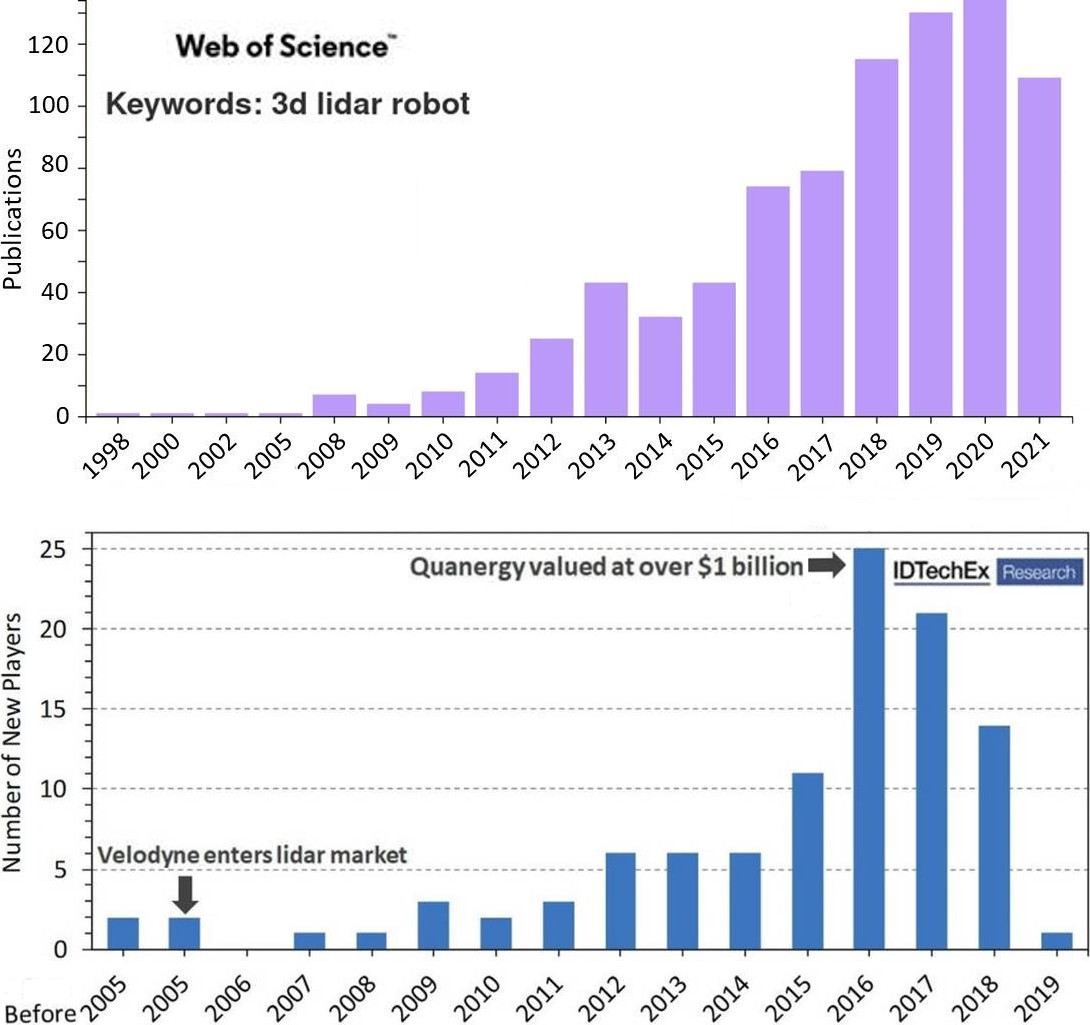
Figure 1: Upper: the results of the number of relevant papers per year searched on the Web of Science with ”3D lidar robot” as the keyword. Lower: new LiDAR manufacturers per year through 2019 [idtechex].

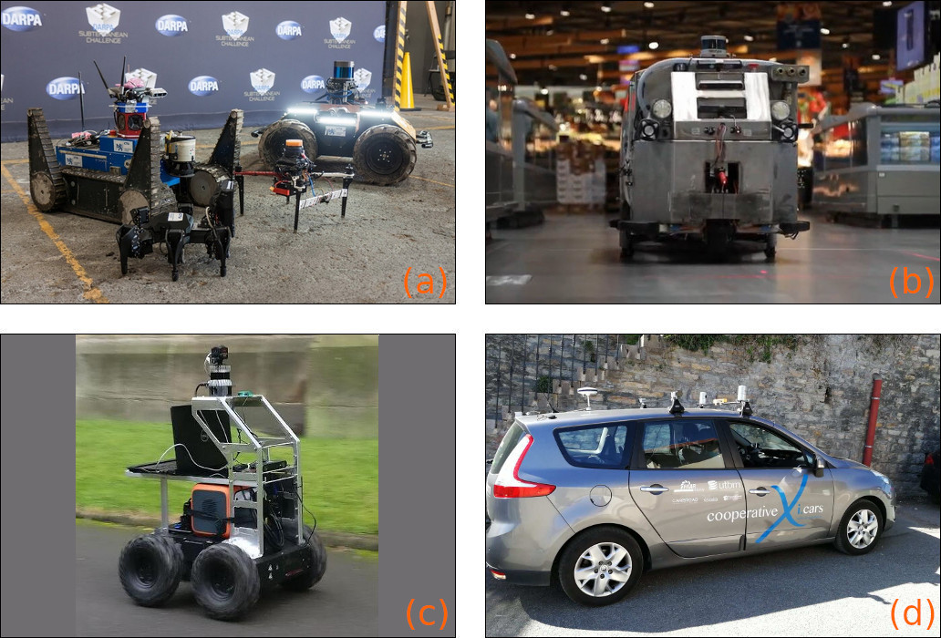
Figure 2: Various LiDARs used in our projects. (a) A RoboSense RS-LiDAR-32 3D LiDAR used by the CTU-CRAS team in the DARPA Sub-T Challenge [DARPA1]. (b) A professional cleaning robot equipped with a Velodyne VLP-16 3D LiDAR [zhimon20jist]. (c) An Ouster OS1-64 3D LiDAR installed on the top of a field robot [ls21iros]. (d) An autonomous car equipped with two Velodyne HDL-32E 3D LiDARs [yz20iros].

This article aims to provide readers with information on the timeliness of 3D time-of-flight (ToF) LiDAR applications in mobile robotics, to classify and analyze research in related fields, and ultimately to provide guidance for deployment of 3D LiDARs in robotic applications. In order to provide a deeper insight in the referenced methods, this article is primarily based on hand-on experience obtained when using 3D LiDARs in the projects we participated in. Therefore, the research axis listed in the following is neither exclusive nor exhaustive. The contributions of this review include:

• An extensive literature survey of 3D LiDAR in the field of mobile robots, focusing primarily on topics related to perception while providing less detailed information to other relevant research (e.g. target tracking, SLAM, etc.).

• A new publicly available benchmark suite for point cloud segmentation, which is based on open source code and open datasets.

The remainder of our review is organized as follows. Section II introduces background knowledge in order to make following this article easier. Section III lists the research that we have focused on in recent years, including object detection, robot localization, long-term robot autonomy, LiDAR data processing under adverse weather conditions, as well as sensor fusion. Section LABEL:sec:applications introduces application areas, including service robots, autonomous driving, and current anti-epidemic deployments. Section LABEL:sec:perspectives provides a vision for future research and development. Section LABEL:sec:conclusions summarizes the full text.

II Preliminaries

II-A Ranging Principle

As mentioned earlier, LiDAR is a surveying method that measures distance to a target by illuminating the target with pulsed laser light and measuring the reflected pulses with a sensor. Fig. 3 shows the working principle of ToF LiDAR. Specifically, the laser transmitter first emits pulsed laser light in a given direction, and when the laser beam encounters an obstacle, it will reflect or diffuse depending on the material on the surface of the object. After the laser detector receives the echo signal, it can determine the distance between the sensor and the object by measuring the time it takes for the laser beam to reach the object from the sensor and then back again. This measurement mechanism can be formulated as:

$$r=\frac{c\cdot\Delta t}{2n}$$ (1)

where $c$ is the speed of light, which is a universal physical constant; $n$ is the refractive index of the propagation medium, which is 1 for air; $\Delta T$ is the time difference between transmitting and receiving laser pulses.

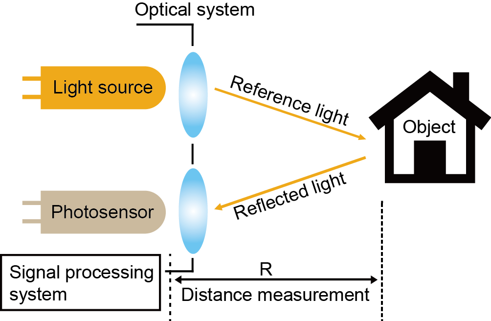
Figure 3: Schematic diagram of the imaging principle of ToF LiDAR.

The reception of a laser beam is not as straightforward as its emission (see Fig. 4). The received laser power function is described by the backscattering coefficient, which can be formulated as [Rasshofer2011]:

$$P_{R}=C\frac{\beta}{R^{2}}\exp\left(-2\int_{r=0}^{R}\alpha(r)dr\right)$$ (2)

where $P_{R}$ is the power of a received laser return at distance $R$; $C$ is the constant related to the light speed, laser transmit power, laser detector’s optical aperture area, and overall system efficiency; $\beta$ is the reflection efficiency of the object surface; $\alpha$ is the extinction coefficient of the LiDAR signal. The advanced signal processing system is required to detect the true return signal in low SNR (Signal-to-Noise Ratio). A typical final stage of the processing pipeline is adaptive thresholding, which takes into account the current background noise [Ogawa2016].

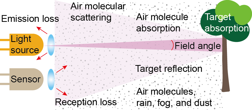
Figure 4: Difficult laser return journey.

II-B Physical Structure

The 3D ToF LiDAR on the market today can be divided into four categories (see Fig. 5) according to the different physical structure of its scanning system, including mechanical rotation, Micro-Electro-Mechanical Systems (MEMS), flash, and Optical Phased Array (OPA), of which the latter three are also called solid-state LiDAR. The mechanical rotation system utilizes a motor to rotate the mirror of the laser beam to obtain a large horizontal Field of View (FoV). By stacking transmitters in the vertical direction or an embedded oscillating lens, lasers in the vertical FoV are generated. MEMS LiDAR uses the electromagnetic force to rotate a micro mirror integrated in the chip to generate dense points at high frequencies in a specific field. It is even possible to control the circuit to generate dense points concentrated in certain specific areas. Flash LiDAR instantly illuminates the scene through the lens. A photodiode array (similar to CMOS) is used to receive the reflected signal to generate a set of 3D points recorded by each pixel. OPA LiDAR realizes scanning in different directions by changing the phase difference of each unit of the laser source array. This type is still in the experimental stage so far. Table I summarizes the advantages and disadvantages of different scanning systems for mass-produced LiDARs. For a detailed physical comparison of different LiDARs, please refer to [you20spm].

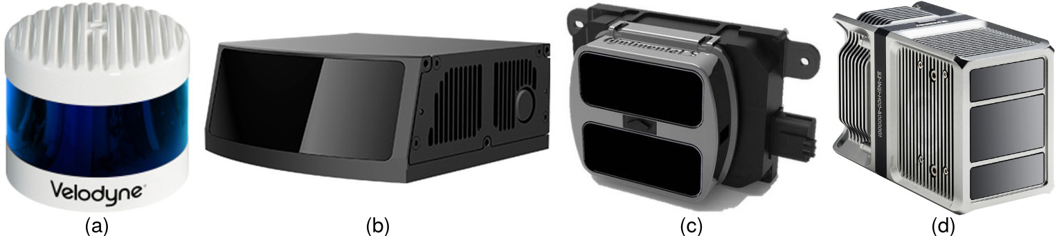
Figure 5: Example products of different types of 3D ToF LiDAR on the market. (a) Velodyne Alpha Prime spanning LiDAR. (b) Robosense M1 MEMS LiDAR. (c) Continental HFL110 3D Flash LiDAR. (d) Quanergy S3-2 OPA LiDAR.

TABLE I: Pros and cons of different categories of 3D ToF LiDAR

Structure	Pros	Cons
Spinning	High technology maturity	Limited life (by wear)
	Up to 360${}^{\circ}$ of horizontal FoV	Large size and high cost
MEMS	Near solid-state structure	Limited detection range
	Small size and low cost	Limited FoV
Flash	Solid-state structure	Low detection range
	Very small size and low cost	Low FoV

For the popular mechanical LiDAR, achieving a higher number of scanning layers needs to stack laser transceiver modules, which means the increasing of both the cost and the difficulty of manufacture. Thus, although the mechanical LiDARs are widely used due to their high technological maturity and 360 degree of horizontal FoV, industry and academia are increasingly investing in MEMS LiDAR, especially in the application and mass production in the field of autonomous driving. However, the small reflection mirror and light receiving aperture limit the detection range of MEMS LiDAR, and transceiver modules and scanning modules still need to be further improved. Flash LiDAR detects the whole area with a single diffused laser, which makes it difficult to achieve a large detection range due to the limitation of laser emission power on human eye safety. Therefore, it is usually used in mid-distance or indoor scenes.

II-C Physical Characteristics

An important specification of LiDAR is the ability to provide fast data collection and high-precision distance measurement. In addition, mechanical rotation-based devices, which are widely used in mobile robotics, can also provide large-scale scans, with up to 360 degrees of horizontal FoV and a measurement distance of tens to hundreds of meters. Furthermore, LiDARs are robust to lighting variations, which makes them more suitable for long-term robot autonomy compared to passive visual sensors. However, the data provided by LiDAR come in a form of a sparse set of points, making objects difficult to identify due to the lack of easy-to-interpret features such as color and texture. This situation usually becomes more serious as the measurement distance increases, because the sensory data becomes sparser with distance. Another limitation of LiDAR is its sensitivity to certain adverse weather conditions. Water droplets in the air have a dual effect on the sensor. First, small droplets in the atmosphere absorb or scatter the near-infrared laser, resulting in an increase in the extinction coefficient $\alpha$ (c.f. Eq. 2). Second, wet surfaces of obstacles lead to weaker reflectivity $\beta$ [Lekner1988]. These factors cause the received laser power to be low, making it impossible to perform the signal processing steps required to detect distant objects. In addition, raindrops and snowflakes near the laser transmitter cause noise and result in false detections [sac2022george]. Table II gives an overview of the performance of commonly used sensors for machine (exteroceptive) perception.

TABLE II: Overview of the performance of commonly used sensors for machine (external) perception

Sensor	LiDAR	Radar	Ultrasonic	Camera
Detection range	$\star\star\star$	$\star\star\star$	$\star$	$\star\star$
Ranging accuracy	$\star\star\star$	$\star\star$	$\star\star$	$\star$
Resolution	$\star\star$	$\star$	$\star$	$\star\star\star$
Horizontal FoV	$\star\star\star$	$\star\star$	$\star$	$\star\star$
Vertical FoV	$\star\star$	$\star$	$\star$	$\star\star$
Color information	$\star\star$	$\star$	$\star$	$\star\star\star$
Lighting robustness	$\star\star\star$	$\star\star\star$	$\star\star\star$	$\star$
Weather robustness	$\star\star$	$\star\star\star$	$\star\star\star$	$\star$

II-D Data Representation and Processing

LiDAR’s knowledge to its surroundings can be represented by a set of points in three-dimensional coordinate space:

$$P=\{p_{i}~{}|~{}p_{i}=(x_{i},y_{i},z_{i})\in\mathbb{R}^{3},i=1,\ldots,I\}$$ (3)

while each point corresponds to a processed laser beam reflection. Conventionally, this set of points is called a point cloud. According to different characteristics of the hardware, additional features might be included, such as intensity and the laser ring number. A point cloud processing library widely used in the field of mobile robotics and autonomous driving is the PCL (Point Cloud Library) [pcl]. This library is open-source, written in C++, based on traditional computer vision algorithms (in contrast to deep neural networks) including feature estimation, surface reconstruction, 3D registration, model fitting, and segmentation. PCD (Point Cloud Data) file format is the point cloud data storage format officially supported by PCL.

Another way to represent and process LiDAR data is inseparable from the well-known Robot Operating System (ROS) [ros]. ROS has become the de facto standard platform for development of software in robotics, and today increasing numbers of researchers and industries develop autonomous driving software based on it. The LiDAR data is usually represented by PointCloud2 ROS message, and can be easily saved and shared via rosbag [yz17iros, yz19auro, yz20iros]. Data processing can be completely handed over to PCL due to the close family relationship between ROS and PCL. In addition, other representations such as binary file (e.g. .bin) [KITTI, oxford-dataset, KAIST, cadcd] and xml file [nuScenes] are also common.

III Research axes

Table III provides the full taxonomic axes from the literature, that will be presented in detail in the following subsections.

TABLE III: Summary of the taxonomic axes

Paper	Axes	Method	Intensity	Ring	3D ToF LiDAR	Usage${}^{1}$	Dataset	OS${}^{2}$
Yan et al. [zhimon20jist]	detection	clustering+SVM${}^{3}$	✓	$\times$	Velodyne VLP-16	combined	FLOBOT	✓
Yan et al. [yz17iros]	detection	clustering+SVM	✓	$\times$	Velodyne VLP-16	alone	L-CAS	✓
Yang et al. [yang21itsc]	detection	online RF${}^{4}$	✓	$\times$	Velodyne HDL-64E	combined	KITTI	✓
Kidono et al. [kidono11iv]	detection	clustering+SVM	✓	$\times$	Velodyne HDL-64E	alone	private	$\times$
Dewan et al. [dewan16icra]	detection	motion curve	$\times$	$\times$	Velodyne HDL-64E	alone	KITTI	$\times$
Zhou and Tuzel [VoxelNet]	detection	DL${}^{5}$	✓	$\times$	Velodyne HDL-64E	alone	KITTI	$\times$
Ali et al. [YOLO3D]	detection	DL	$\times$	$\times$	Velodyne HDL-64E	alone	KITTI	$\times$
N-Serment et al. [navarro-serment09fsr]	detection	tracking+SVM	$\times$	$\times$	unknown	alone	private	$\times$
Häselich et al. [haselich14iros]	detection	clustering+SVM	$\times$	$\times$	Velodyne HDL-64E	alone	Freiburg+private	$\times$
Li et al. [li16its]	detection	clustering+SVM	$\times$	$\times$	Velodyne HDL-64E	alone	private	$\times$
Wang and Posner [wang15rss]	detection	SW${}^{6}$+SVM	✓	$\times$	Velodyne HDL-64E	alone	KITTI	$\times$
Spinello et al. [spinello11icra]	detection	clustering+AB${}^{7}$	$\times$	$\times$	Velodyne HDL-64E	alone	Freiburg	$\times$
Deuge et al. [deuge13acra]	detection	clustering+SVM	✓	$\times$	Velodyne HDL-64E	alone	Sydney Urban	$\times$
Teichman and Thrun [teichman12ijrr]	detection	clustering+EM${}^{8}$	$\times$	$\times$	Velodyne HDL-64E	alone	Stanford	$\times$
Dequaire et al. [dequaire17ijrr]	detection	DL	$\times$	$\times$	Velodyne HDL-64E	alone	Oxford	$\times$
Sualeh and Kim [sualeh19sensor]	detection	clustering+TM${}^{9}$	$\times$	$\times$	Velodyne HDL-64E	alone	KITTI	$\times$
Qi et al. [qi21cvpr]	detection	DL	✓	$\times$	unkown	alone	Waymo	$\times$
Yan et al. [yz18iros]	detection	clustering+SVM	✓	$\times$	Velodyne VLP-16	combined	L-CAS MS	✓
Sun et al. [ls20icra]	localization	DL	$\times$	$\times$	Velodyne HDL-32E	alone	NCLT	$\times$
Wang et al. [wang2020pointloc]	localization	DL	$\times$	$\times$	Velodyne HDL-32E	alone	Oxford	$\times$
Dubé et al. [dube2017segmatch]	localization	RF+NN${}^{10}$	$\times$	$\times$	Velodyne HDL-64E	alone	KITTI	✓
Dubé et al. [segmap2018]	localization	DL+NN	$\times$	$\times$	Velodyne HDL-64E	alone	KITTI+private	✓
Tinchev et al. [tinchev2019learning]	localization	DL	$\times$	$\times$	Velodyne 64, 32, 16	alone	KITTI+private	$\times$
Kong et al. [kong2020semantic]	localization	DL+NN	$\times$	$\times$	Velodyne HDL-64E	alone	KITTI	✓
He et al. [he2016m2dp]	localization	heuristic	$\times$	✓	Velodyne HDL-64E	alone	KITTI+others	✓
Kim and Kim [kim2018scan]	localization	heuristic	$\times$	✓	Velodyne 64,32,16	alone	KITTI+others	✓
Cop et al. [cop2018delight]	localization	heuristic	✓	$\times$	Velodyne VLP-16	alone	private	$\times$
Kim et al. [kim20191]	localization	DL	$\times$	✓	Velodyne HDL-32E	alone	NCLT, Oxford	✓
Chen et al. [chen2020overlapnet]	localization	DL	✓	$\times$	Velodyne HDL-64E	alone	KITTI, Ford	✓
Uy and Lee [angelina2018pointnetvlad]	localization	DL	$\times$	$\times$	Velodyne HDL-64E	alone	Oxford+private	✓
Liu et al. [liu2019lpd]	localization	DL	$\times$	$\times$	Velodyne HDL-64E	alone	Oxford+private	✓
Kucner et al. [kucnerconditional]	long-term	grid-based	$\times$	$\times$	Velodyne HDL-64E	alone	private	$\times$
Pomerleau et al. [pomerleau2014long]	long-term	heuristic	$\times$	$\times$	Velodyne HDL-32E	alone	private	$\times$
Sun et al. [ls18icra]	long-term	DL	$\times$	$\times$	Velodyne VLP-16	combined	L-CAS	$\times$
Sun et al. [ls18ral]	long-term	DL	$\times$	$\times$	Velodyne HDL-32E	alone	private	$\times$
Vintr et al. [vintr19ecmr]	long-term	benchmarking	✓	$\times$	Velodyne VLP-16	alone	L-CAS	$\times$
Vintr et al. [vintr19icra]	long-term	hypertime	✓	$\times$	Velodyne VLP-16	alone	L-CAS	$\times$
Vintr et al. [vintr20iros]	long-term	benchmarking	✓	$\times$	Velodyne HDL-32E	alone	private	$\times$
Broughton et al. [broughton2020learning]	long-term	DL+SVM	$\times$	$\times$	Velodyne VLP-16	combined	private	$\times$
Rasshofer et al. [Rasshofer2011]	weather	physical model	✓	$\times$	unknown	alone	private	$\times$
Roy et al. [roy2020physical]	weather	physical model	✓	$\times$	unknown	alone	private	$\times$
Yang et al. [yang20iros]	weather	GPR${}^{11}$+DL	✓	$\times$	Velodyne VLP-32C	alone	private	✓
Hahner et al. [hahner2021fog]	weather	physical model	✓	$\times$	Velodyne 64, 32	alone	DENSE/STF	✓
Charron et al. [8575761]	weather	distance-based	$\times$	$\times$	Velodyne VLP-32C	alone	CADC	✓
Heinzler et al. [heinzler2020cnn]	weather	DL	✓	$\times$	Velodyne VLP-32C	alone	DENSE/STF	✓
JI-IL et al. [park2020fast]	weather	intensity-based	✓	$\times$	Ouster OS-1 64	alone	private	$\times$
Kurup et al. [kurup2021dsor]	weather	distance-based	$\times$	$\times$	unkown	alone	WADS	✓

${}^{1}$Can be used alone or need to be fused with other modal sensors. ${}^{2}$Open Source. ${}^{3}$Support Vector Machine. ${}^{4}$Random Forest. ${}^{5}$Deep Learning.
${}^{6}$Sliding Window. ${}^{7}$AdaBoost. ${}^{8}$Expectation Maximization. ${}^{9}$Template Matching. ${}^{10}$Nearest Neighbor. ${}^{11}$Gaussian Process Regression.