An accelerated proximal gradient method for multiobjective optimization

Abstract

This paper presents an accelerated proximal gradient method for multiobjective optimization, in which each objective function is the sum of a continuously differentiable, convex function and a closed, proper, convex function. Extending first-order methods for multiobjective problems without scalarization has been widely studied, but providing accelerated methods with accurate proofs of convergence rates remains an open problem. Our proposed method is a multiobjective generalization of the accelerated proximal gradient method, also known as the Fast Iterative Shrinkage-Thresholding Algorithm (FISTA), for scalar optimization. The key to this successful extension is solving a subproblem with terms exclusive to the multiobjective case. This approach allows us to demonstrate the global convergence rate of the proposed method ($O(1/k^{2})$), using a merit function to measure the complexity. Furthermore, we present an efficient way to solve the subproblem via its dual representation, and we confirm the validity of the proposed method through some numerical experiments.

1 Introduction

Multiobjective optimization consists in minimizing (or maximizing) more than one objective function at once under possible constraints. In general, there is no single point that minimizes all objective functions simultaneously, so the concept of Pareto optimality becomes essential. We call a point Pareto optimal if there is no other point with the same or smaller objective function values and with at least one objective function value being strictly smaller.

One of the most popular strategies for solving multiobjective optimization problems is the scalarization approach [23, 24, 46]. It converts the original multiobjective problem into another, which has a parametrized scalar-valued objective function. If each objective function in the multiobjective optimization problem is convex, the converted single objective optimization problems typically become convex optimization. However, it can be challenging to choose the appropriate parameters (or weights) in advance. For example, Marler and Arora [30] discussed such difficulties in the weighted sum method. Another approach, which does not use scalarization, is based on metaheuristics [22] but lacks a theoretical proof of convergence to Pareto solutions.

To overcome those drawbacks, many descent algorithms for multiobjective optimization problems have been developed recently [21]. These algorithms decrease all objective functions at each iteration, offer the advantages of not requiring a priori parameter selection, and provide convergence guarantees under reasonable assumptions. For instance, Fliege and Svaiter [18] proposed the steepest descent method for differentiable multiobjective optimization problems. Other examples include the projected gradient [20, 26, 47], Newton’s [17, 25], trust-region [12], and conjugate gradient methods [29]. Descent methods for infinite-dimensional vector optimization problems have also been studied, including the proximal point [7] and the inertial forward-backward methods [5]. Among these, methods that use only the first-order derivatives of the objective functions, such as the steepest descent and the projected gradient methods, are called first-order methods. Another well-known multiobjective first-order method is the proximal gradient [40], which works for composite problems, i.e., with each objective being the sum of a differentiable function and a convex but not necessarily differentiable one. This algorithm, as well as the steepest descent, is known to converge to Pareto solutions with rate $O(1/k)$ [19, 41].

On the other hand, there are many studies related to the acceleration of single-objective first-order methods. After being established by Nesterov [34], researchers developed various accelerated schemes. In particular, the Fast Iterative Shrinkage-Thresholding Algorithm (FISTA) [3], an accelerated version of the proximal gradient method, has contributed to a wide range of research fields, including image and signal processing. These methods may increase the objective function values in some iterations, but overall they are known to converge faster than the original descent methods, both theoretically and experimentally.

However, in the multiobjective case, the studies associated with accelerated algorithms are still insufficient [16, 44]. In 2020, El Moudden and El Mouatasim [16] proposed an accelerated diagonal steepest descent method for multiobjective optimization, a natural extension of Nesterov’s accelerated method for single-objective problems. They proved the global convergence rate of the algorithm ($O(1/k^{2})$) under the assumption that the sequence of the Lagrange multipliers of the subproblems is eventually fixed. Nevertheless, this assumption is restrictive because it indicates that the approach is essentially the same as the (single-objective) Nesterov’s method, only applied to the minimization of a weighted sum of the objective functions.

Here, we propose a genuine accelerated proximal gradient method for multiobjective optimization. As it is usual, in each iteration, we solve a convex (scalar-valued) subproblem. While the accelerated and non-accelerated algorithms solve the same subproblem in the single-objective case, the subproblem of our accelerated method has terms that are not included in the non-accelerated version. However, we can ignore these terms in the single-objective case, and thus we can regard our proposed method as a generalization of FISTA. Moreover, under more natural assumptions, we prove the proposed method’s global convergence rate ($O(1/k^{2})$) by using a merit function [42] to measure the complexity.

Furthermore, having the practical computational efficiency in mind, we derive a dual of the subproblem, which is convex and differentiable. Such a dual problem turns out to be easier to solve than the original one, especially when the number of objective functions is smaller than the dimension of the decision variables. We can also reconstruct the original subproblem’s solution directly from the dual optimum. In addition, we implement the whole algorithm using this dual problem and confirm its effectiveness with numerical experiments.

The outline of this paper is as follows. In Section 2, we introduce some notations and concepts used in this paper. Section 3 recalls the proximal gradient method for multiobjective optimization proposed in [40]. We present the proposed accelerated proximal gradient method for multiobjective optimization in Section 4 and analyze its $O(1/k^{2})$ convergence rate in Section 5. Moreover, Section 6 introduces an efficient way to solve the subproblem via its dual form. Finally, we report some numerical results for test problems in Section 7, demonstrating that the proposed method is faster than the one without acceleration.

2 Preliminaries

All over this work, for any natural number $d$, $\mathbf{R}^{d}$ denotes the $d$-dimensional real space, $\mathbf{R}_{\mathord{+}}^{d}\subseteq\mathbf{R}^{d}$ designates the nonnegative orthant of $\mathbf{R}^{d}$, i.e.,$\mathbf{R}_{\mathord{+}}^{d}\coloneqq\left\{v\in\mathbf{R}^{d}\mathrel{}\middle|\mathrel{}v_{i}\geq 0,i=1,\dots,d\right\}$, and $\Delta^{d}$ represents the standard simplex in $\mathbf{R}^{d}$ given by

$$\Delta^{d}\coloneqq\left\{\lambda\in\mathbf{R}_{\mathord{+}}^{d}\mathrel{}\middle|\mathrel{}\sum_{i=1}^{d}\lambda_{i}=1\right\}.$$

Then, we can consider the partial orders induced by $\mathbf{R}_{\mathord{+}}^{d}$: for all $v^{1},v^{2}\in\mathbf{R}^{d}$, $v^{1}\leq v^{2}$ (alternatively, $v^{2}\geq v^{1}$) if $v^{2}-v^{1}\in\mathbf{R}_{\mathord{+}}^{d}$ and $v^{1}<v^{2}$ (alternatively, $v^{2}>v^{1}$) if $v^{2}-v^{1}\in\operatorname{int}\mathbf{R}_{\mathord{+}}^{d}$. In other words, $v^{1}\leq v^{2}$ and $v^{1}<v^{2}$ stand for $v^{1}_{i}\leq v^{2}_{i}$ and $v^{1}_{i}<v^{2}_{i}$ for all $i=1,\dots,d$, respectively. Moreover, let $\left\langle\cdot,\cdot\right\rangle$ be the Euclidean inner product in $\mathbf{R}^{d}$, i.e., $\left\langle u,v\right\rangle\coloneqq\sum_{i=1}^{d}{u_{i}v_{i}}$, and let $\left\lVert\cdot\right\rVert$ be the Euclidean norm, i.e., $\left\lVert u\right\rVert\coloneqq\sqrt{\left\langle u,u\right\rangle}$. Furthermore, we define the $\ell_{1}$-norm and the $\ell_{\infty}$-norm by $\left\lVert u\right\rVert_{1}\coloneqq\sum_{i=1}^{d}\left\lvert u_{i}\right\rvert$ and $\left\lVert u\right\rVert_{\infty}\coloneqq\max_{i=1,\dots,d}\left\lvert u_{i}\right\rvert$, respectively. We now recall the obvious equality related to norm and inner product:

$$\lVert b-a\rVert^{2}+2\langle b-a,a-c\rangle=\lVert b-c\rVert^{2}-\lVert a-c\rVert^{2}\quad\text{for all~{}$a,b,c\in\mathbf{R}^{n}$}.$$

On the other hand, for a closed, proper and convex function $h\colon\mathbf{R}^{n}\to\mathbf{R}\cup\left\{+\infty\right\}$, we call $\eta\in\mathbf{R}^{n}$ a subgradient of $h$ at $x\in\mathbf{R}^{n}$ if

$$h(y)\geq h(x)+\left\langle\eta,y-x\right\rangle\quad\text{for all~{}$y\in\mathbf{R}^{n}$},$$

and we write $\partial h(x)$ the subdifferential of $h$ at $x$, i.e., the set of all subgradients of $h$ at $x$. In addition, the subdifferential for a vector-valued function is the direct product of the subdifferentials of each component. We also define the Moreau envelope or Moreau-Yosida regularization [33, 45] of $h$ by

$$\operatorname{\mathcal{M}}_{h}(x)\coloneqq\min_{y\in\mathbf{R}^{n}}\left[h(y)+\frac{1}{2}\left\lVert x-y\right\rVert^{2}\right].$$

The minimization problem in Section 2 has a unique solution because of the strong convexity of its objective function. We call this solution the proximal operator and write it as

$$\operatorname{\mathbf{prox}}_{h}(x)\coloneqq\operatorname*{argmin}_{y\in\mathbf{R}^{n}}\left[h(y)+\frac{1}{2}\left\lVert x-y\right\rVert^{2}\right].$$

Remark 2.1.

1. [2, Theorem 6.24] If $h$ is the indicator function of a nonempty set $S\subseteq\mathbf{R}^{n}$, i.e.,

   $$\operatorname{\chi}_{S}(x)=\begin{dcases}0,&x\in S,\\ +\infty,&x\notin S,\end{dcases}$$

   then the proximal operator reduces to the projection onto $S$.

2. [2, Theorem 6.42] The proximal operator of a closed, proper, and convex function $h$ is non-expansive, i.e., $\left\lVert\operatorname{\mathbf{prox}}_{h}(x)-\operatorname{\mathbf{prox}}_{h}(y)\right\rVert\leq\left\lVert x-y\right\rVert$. In other words, $\operatorname{\mathbf{prox}}_{h}$ is $1$-Lipschitz continuous.

3. [2, Theorem 6.60] Even if a closed, proper, and convex function $h$ is non-differentiable, its Moreau envelope $\operatorname{\mathcal{M}}_{h}$ has a $1$-Lipschitz continuous gradient as follows: $\nabla\operatorname{\mathcal{M}}_{h}(x)=x-\operatorname{\mathbf{prox}}_{h}(x)$.

We now focus on the following multiobjective optimization problem:

$$\min_{x\in\mathbf{R}^{n}}\quad F(x)$$

with a vector-valued function $F\colon\mathbf{R}^{n}\to(\mathbf{R}\cup\{+\infty\})^{m}$ with $F\coloneqq(F_{1},\dots,F_{m})^{\top}$. We assume that each component $F_{i}\colon\mathbf{R}^{n}\to\mathbf{R}\cup\{+\infty\}$ is defined by $F_{i}(x)\coloneqq f_{i}(x)+g_{i}(x)$ for all $i=1,\dots,m$ with convex and continuously differentiable functions $f_{i}\colon\mathbf{R}^{n}\to\mathbf{R},i=1,\dots,m$ and closed, proper and convex functions $g_{i}\colon\mathbf{R}^{n}\to\mathbf{R}\cup\left\{+\infty\right\},i=1,\dots,m$. We also suppose that each $\nabla f_{i}$ is Lipschitz continuous with constant $L_{i}>0$ and define $L\coloneqq\max_{i=1,\dots,m}{L_{i}}$. From the so-called descent lemma [4, Proposition A.24], we have $f_{i}(p)-f_{i}(q)\leq\left\langle\nabla f_{i}(q),p-q\right\rangle+(L/2)\left\lVert p-q\right\rVert^{2}$ for all $p,q\in\mathbf{R}^{n}$ and $i=1,\dots,m$, which gives

$$F_{i}(p)-F_{i}(r) =f_{i}(p)-f_{i}(q)+g_{i}(p)+f_{i}(q)-F_{i}(r)$$

$$\leq\left\langle\nabla f_{i}(q),p-q\right\rangle+g_{i}(p)+f_{i}(q)-F_{i}(r)+\frac{L}{2}\left\lVert p-q\right\rVert^{2}$$

for all $p,q,r\in\mathbf{R}^{n}$ and $i=1,\dots,m$.

Now, we introduce some concepts used in the multiobjective optimization problem Section 2. Recall that

$$X^{\ast}\coloneqq\left\{x^{\ast}\in\mathbf{R}^{n}\mathrel{}\middle|\mathrel{}\text{There does not exist~{}$x\in\mathbf{R}^{n}$ such that~{}$F(x)<F(x^{\ast})$}\right\}$$

is the set of weakly Pareto optimal points for Section 2. We also define the effective domain of $F$ by $\operatorname{dom}F\coloneqq\left\{x\in\mathbf{R}^{n}\mathrel{}\middle|\mathrel{}F_{i}(x)<+\infty\text{ for all }i=1,\dots,m\right\}$, and we write the level set of $F$ on $c\in\mathbf{R}^{m}$ as

$$\mathcal{L}_{F}(c)\coloneqq\left\{x\in\mathbf{R}^{n}\mathrel{}\middle|\mathrel{}F(x)\leq c\right\}.$$

In addition, we express the image of $A\subseteq\mathbf{R}^{n}$ and the inverse image of $B\subseteq(\mathbf{R}\cup\left\{+\infty\right\})^{m}$ under $F$ as $F(A)\coloneqq\left\{F(x)\in\mathbf{R}^{m}\mathrel{}\middle|\mathrel{}x\in A\right\}\quad\text{and}\quad F^{-1}(B)\coloneqq\left\{x\in\mathbf{R}^{n}\mathrel{}\middle|\mathrel{}F(x)\in B\right\}$, respectively.

Finally, let us recall the merit function $u_{0}\colon\mathbf{R}^{n}\to\mathbf{R}\cup\left\{+\infty\right\}$ proposed in [42]:

$$u_{0}(x)\coloneqq\sup_{z\in\mathbf{R}^{n}}\min_{i=1,\dots,m}[F_{i}(x)-F_{i}(z)],$$

which returns zero at optimal solutions and strictly positive values otherwise. The following theorem shows that $u_{0}$ is a merit function in the Pareto sense.

Theorem 2.1.

[42, Theorem 3.1] Let $u_{0}$ be defined by Section 2. Then, we get $u_{0}(x)\geq 0$ for all $x\in\mathbf{R}^{n}$. Moreover, $x\in\mathbf{R}^{n}$ is weakly Pareto optimal for Section 2 if and only if $u_{0}(x)=0$.

Note that when $m=1$, we have $u_{0}(x)=F_{1}(x)-F_{1}^{\ast}$, where $F_{1}^{\ast}$ is the optimal objective value. This is clearly a merit function for scalar-valued optimization.

3 Proximal gradient methods for multiobjective optimization

Let us now recall the proximal gradient method for Section 2, an extension of the classical proximal gradient method, proposed by Tanabe, Fukuda, and Yamashita [40]. We explain how to generate the sequence of iterates, and afterward, we show the algorithm and its convergence rate.

For given $x\in\operatorname{dom}F$ and $\ell>0$, we consider the following minimization problem:

$$\min_{z\in\mathbf{R}^{n}}\quad\varphi_{\ell}(z;x),$$

where $\varphi_{\ell}(z;x)\coloneqq\max_{i=1,\dots,m}[\left\langle\nabla f_{i}(x),z-x\right\rangle+g_{i}(z)-g_{i}(x)]+(\ell/2)\lVert z-x\rVert^{2}$. The convexity of $g_{i}$ implies that $z\mapsto\varphi_{\ell}(z;x)$ is strongly convex, so the problem Section 3 always has a unique solution. Let us write such a solution as $p_{\ell}(x)$ and let $\theta_{\ell}(x)$ be its optimal function value, i.e.,

$$p_{\ell}(x)\coloneqq\operatorname*{argmin}_{z\in\mathbf{R}^{n}}{\varphi_{\ell}(z;x)}\quad\text{and}\quad\theta_{\ell}(x)\coloneqq\min_{z\in\mathbf{R}^{n}}\varphi_{\ell}(z;x).$$

The following proposition shows that $p_{\ell}(x)$ and $\theta_{\ell}(x)$ helps to characterize the weak Pareto optimality of Section 2.

Proposition 3.1.

Let $p_{\ell}$ and $\theta_{\ell}$ be defined by Section 3. Then, the statements below hold.

1. The following three conditions are equivalent: (a) $x$is weakly Pareto optimal; (b) $p_{\ell}(x)=x$; (c) $\theta_{\ell}(x)=0$.

2. The mappings $p_{\ell}$ and $\theta_{\ell}$ are both continuous.

Proof.

It is clear from [40, Lemma 3.2] and the convexity of $f_{i}$. ∎

From Proposition 3.1, we can treat $\left\lVert p_{\ell}(x)-x\right\rVert_{\infty}<\varepsilon$ for some $\varepsilon>0$ as a stopping criteria. Moreover, if $\ell>L/2$ then we have $F_{i}(p_{\ell}(x))\leq F_{i}(x)$ for all $x\in\operatorname{dom}F$ and $i=1,\dots,m$ [41]. Now, we state below the proximal gradient method for Section 2.

Algorithm 1 Proximal gradient method for multiobjective optimization [40]

1:$x^{0}\in\operatorname{dom}F$, $\ell>L/2$, $\varepsilon>0$

2:$x^{\ast}$: A weakly Pareto optimal point

3:$k\leftarrow 0$

4:loop

5:     $x^{k+1}\leftarrow p_{\ell}(x^{k})$, where $p_{\ell}$ is defined by Section 3

6:     if $\left\lVert x^{k+1}-x^{k}\right\rVert_{\infty}\geq\varepsilon$ then return $x^{k+1}$

7:     end if

8:     $k\leftarrow k+1$

9:end loop

When $\ell\geq L$, Algorithm 1 is known to generate $\{x^{k}\}$ such that $\{u_{0}(x^{k})\}$ converges to zero with rate $O(1/k)$ under the following assumption. Note that this assumption is not particularly strong, as suggested in [41, Remark 5.2].

Assumption 3.1.

[41, Assumption 5.1] Let $X^{\ast}$ and $\mathcal{L}_{F}$ be defined by Sections 2 and 2, respectively. Then, for all $x\in\mathcal{L}_{F}(F(x^{0}))$, there exists $x^{\ast}\in X^{\ast}$ such that $F(x^{\ast})\leq F(x)$ and

$$R\coloneqq\sup_{F^{\ast}\in F(X^{\ast}\cap\mathcal{L}_{F}(F(x^{0})))}\inf_{z\in F^{-1}(\left\{F^{\ast}\right\})}\left\lVert z-x^{0}\right\rVert^{2}<+\infty.$$

Theorem 3.1.

[41, Theorem 5.2] Assume that $\ell\geq L$. Then, under Assumption 3.1, Algorithm 1 generates a sequence $\{x^{k}\}$ such that $u_{0}(x^{k})\leq(\ell R)/(2k)$ for all $k\geq 1$.

At the end of this section, we note some remarks about Algorithm 1.

Remark 3.1.

1. Since $x\in\operatorname{dom}F$ implies $p_{\ell}(x)\in\operatorname{dom}F$, Algorithm 1 is well-defined.

2. If $g_{i}=0$, Algorithm 1 corresponds to the steepest descent method [18]:

   $$x^{k+1}\coloneqq\min_{z\in\mathbf{R}^{n}}\left[\max_{i=1,\dots,m}\left\langle\nabla f_{i}(x^{k}),z-x^{k}\right\rangle+\frac{\ell}{2}\left\lVert z-x^{k}\right\rVert^{2}\right].$$

   On the other hand, when $f_{i}=0$, it matches the proximal point method [7]:

   $$x^{k+1}\coloneqq\min_{z\in\mathbf{R}^{n}}\left\{\max_{i=1,\dots,m}\left[g_{i}(z)-g_{i}(x)\right]+\frac{\ell}{2}\left\lVert z-x^{k}\right\rVert^{2}\right\}.$$

   Furthermore, when $g_{i}$ is the indicator function Remark 2.1 (i) of a convex set $S\subseteq\mathbf{R}^{n}$, it coincides with the projected gradient method [26]:

   $$x^{k+1}\coloneqq\min_{z\in S-x^{k}}\left[\max_{i=1,\dots,m}\left\langle\nabla f_{i}(x^{k}),z-x^{k}\right\rangle+\frac{\ell}{2}\left\lVert z-x^{k}\right\rVert^{2}\right].$$

3. When it is difficult to estimate the Lipschitz constant $L$, we can set the initial value of $\ell$ appropriately. Then, at each iteration we increase $\ell$ by multiplying it with some prespecified scalar, until $F_{i}(p_{\ell}(x^{k}))-F_{i}(x^{k})\leq\theta_{\ell}(x^{k})$ is satisfied for all $i=1,\dots,m$. If $L$ is finite, the number of times that $\ell$ is increased is at most a constant.

4 An accelerated proximal gradient method for multiobjective optimization

This section proposes an accelerated version of the proximal gradient method for multiobjective optimization. Similarly to the non-accelerated version given in the last section, a subproblem is considered in each iteration. More specifically, the proposed method solves the following subproblem for given $x\in\operatorname{dom}F$, $y\in\mathbf{R}^{n}$, and $\ell\geq L$:

$$\min_{z\in\mathbf{R}^{n}}\quad\varphi^{\mathrm{acc}}_{\ell}(z;x,y),$$

where

$$\varphi^{\mathrm{acc}}_{\ell}(z;x,y)\coloneqq\max_{i=1,\dots,m}\left[\langle\nabla f_{i}(y),z-y\rangle+g_{i}(z)+f_{i}(y)-F_{i}(x)\right]+\frac{\ell}{2}\lVert z-y\rVert^{2}.$$

Note that when $y=x$, Section 4 is reduced to the subproblem Section 3 of the proximal gradient method. Note also that when $m=1$, the subproblem becomes

$$\min_{z\in\mathbf{R}^{n}}\quad\left\langle\nabla f_{1}(y),z-y\right\rangle+g_{1}(z)+\frac{\ell}{2}\lVert z-y\rVert^{2},$$

which is the subproblem of the single-objective FISTA [3]. The distinctive feature of our proposal Section 4 is the term $f_{i}(y)-F_{i}(x)$, whereas the easy analogy from the single-objective subproblem Section 4 is

$$\min_{z\in\mathbf{R}^{n}}\quad\max_{i=1,\dots,m}\left[\langle\nabla f_{i}(y),z-y\rangle+g_{i}(z)\right]+\frac{\ell}{2}\lVert z-y\rVert^{2}.$$

By putting such a term, the inside of the $\max$ operator approximates $F_{i}(z)-F_{i}(x)$ rather than $F_{i}(z)-F_{i}(y)$. This is a negligible difference in the single-objective case, but deeply affects the proof in the multi-objective case.

Since $g_{i}$ is convex for all $i=1,\dots,m$, $z\mapsto\varphi^{\mathrm{acc}}_{\ell}(z;x,y)$ is strongly convex. Thus, the subproblem Section 4 has a unique optimal solution $p^{\mathrm{acc}}_{\ell}(x,y)$ and takes the optimal function value $\theta^{\mathrm{acc}}_{\ell}(x,y)$, i.e.,

$$p^{\mathrm{acc}}_{\ell}(x,y)\coloneqq\operatorname*{argmin}_{z\in\mathbf{R}^{n}}\varphi^{\mathrm{acc}}_{\ell}(z;x,y)\quad\text{and}\quad\theta^{\mathrm{acc}}_{\ell}(x,y)\coloneqq\min_{z\in\mathbf{R}^{n}}\varphi^{\mathrm{acc}}_{\ell}(z;x,y).$$

Moreover, the optimality condition of Section 4 implies that for all $x\in\operatorname{dom}F$ and $y\in\mathbf{R}^{n}$ there exists $\eta(x,y)\in\partial g(p^{\mathrm{acc}}_{\ell}(x,y))$ and a Lagrange multiplier $\lambda(x,y)\in\mathbf{R}^{m}$ such that

$$\sum_{i=1}^{m}\lambda_{i}(x,y)\left[\nabla f_{i}(y)+\eta_{i}(x,y)\right]=-\ell\left[p^{\mathrm{acc}}_{\ell}(x,y)-y\right]$$ (1a)

$$\lambda(x,y)\in\Delta^{m},\quad\lambda_{j}(x,y)=0\quad\text{for all~{}$j\notin\mathcal{I}(x,y)$},$$ (1b)

where $\Delta^{m}$ denotes the standard simplex Section 2 and

$$\mathcal{I}(x,y)\coloneqq\operatorname*{argmax}_{i=1,\dots,m}\left[\langle\nabla f_{i}(y),p^{\mathrm{acc}}_{\ell}(x,y)-y\rangle+g_{i}(p^{\mathrm{acc}}_{\ell}(x,y))+f_{i}(y)-F_{i}(x)\right].$$

Now, we introduce a relation useful for the subsequent analysis.

Lemma 4.1.

Let $p^{\mathrm{acc}}_{\ell}$ and $\theta^{\mathrm{acc}}_{\ell}$ be defined by Section 4. Then, we have

$$-\frac{\ell}{2}\left[\lVert p^{\mathrm{acc}}_{\ell}(x,y)-z\rVert^{2}-\lVert y-z\rVert^{2}\right]$$ (2)

$$\geq\theta^{\mathrm{acc}}_{\ell}(x,y)+\sum_{i=1}^{m}\lambda_{i}(x,y)\left[\langle\nabla f_{i}(y),y-z\rangle-g_{i}(z)-f_{i}(y)+F_{i}(x)\right]$$ (3)

for all $x,z\in\operatorname{dom}F$ and $y\in\mathbf{R}^{n}$.

Proof.

Let $x,z\in\operatorname{dom}F$ and $y\in\mathbf{R}^{n}$. From 1a and the definition Section 2 of the subgradient, we get

$$-\ell\langle p^{\mathrm{acc}}_{\ell}(x,y)-y,p^{\mathrm{acc}}_{\ell}(x,y)-z\rangle$$ (4)

$$\geq{} \sum_{i=1}^{m}\lambda_{i}(x,y)\left[\langle\nabla f_{i}(y),p^{\mathrm{acc}}_{\ell}(x,y)-z\rangle+g_{i}(p^{\mathrm{acc}}_{\ell}(x,y))-g_{i}(z)\right]$$ (5)

$$={} \sum_{i=1}^{m}\lambda_{i}(x,y)\left[\langle\nabla f_{i}(y),p^{\mathrm{acc}}_{\ell}(x,y)-y\rangle+g_{i}(p^{\mathrm{acc}}_{\ell}(x,y))+f_{i}(y)-F_{i}(x)\right]$$ (6)

$$+\sum_{i=1}^{m}\lambda_{i}(x,y)\left[\langle\nabla f_{i}(y),y-z\rangle-g_{i}(z)-f_{i}(y)+F_{i}(x)\right]$$ (7)

$$={} \max_{i=1,\dots,m}\left[\langle\nabla f_{i}(y),p^{\mathrm{acc}}_{\ell}(x,y)-y\rangle+g_{i}(p^{\mathrm{acc}}_{\ell}(x,y))+f_{i}(y)-F_{i}(x)\right]$$ (8)

$$+\sum_{i=1}^{m}\lambda_{i}(x,y)\left[\langle\nabla f_{i}(y),y-z\rangle-g_{i}(z)-f_{i}(y)+F_{i}(x)\right],$$ (9)

where the second equality comes from 1b and 4. Adding $(\ell/2)\lVert p^{\mathrm{acc}}_{\ell}(x,y)-y\rVert^{2}$ to both sides and the definition Section 4 of $p^{\mathrm{acc}}_{\ell}$ and $\theta^{\mathrm{acc}}_{\ell}$ lead to

$$-\frac{\ell}{2}\left[2\langle p^{\mathrm{acc}}_{\ell}(x,y)-y,p^{\mathrm{acc}}_{\ell}(x,y)-z\rangle-\lVert p^{\mathrm{acc}}_{\ell}(x,y)-y\rVert^{2}\right]$$ (10)

$$\geq\theta^{\mathrm{acc}}_{\ell}(x,y)+\sum_{i=1}^{m}\lambda_{i}(x,y)\left[\langle\nabla f_{i}(y),y-z\rangle-g_{i}(z)-f_{i}(y)+F_{i}(x)\right].$$ (11)

The left-hand side of this inequality is equal to $-(\ell/2)[2\langle p^{\mathrm{acc}}_{\ell}(x,y)-y,y-z\rangle+\lVert p^{\mathrm{acc}}_{\ell}(x,y)-y\rVert^{2}]$. Hence, applying Section 2 with $(a,b,c)\coloneqq(y,z,p^{\mathrm{acc}}_{\ell}(x,y))$, we get the desired inequality. ∎

We also note that by taking $z=y$ in the objective function of Section 4, we have

$$\theta^{\mathrm{acc}}_{\ell}(x,y)\leq\varphi^{\mathrm{acc}}_{\ell}(y;x,y)=\max_{i=1,\dots,m}\left\{F_{i}(y)-F_{i}(x)\right\}$$

for all $x\in\operatorname{dom}F$ and $y\in\mathbf{R}^{n}$. Moreover, from Section 2 with $p=z,q=y,r=x$, and the fact that $\ell\geq L$, it follows that

$$\theta^{\mathrm{acc}}_{\ell}(x,y)\geq\max_{i=1,\dots,m}\left\{F_{i}(p^{\mathrm{acc}}_{\ell}(x,y))-F_{i}(x)\right\}$$

for all $x\in\operatorname{dom}F$ and $y\in\mathbf{R}^{n}$. We now characterize weak Pareto optimality in terms of the mappings $p^{\mathrm{acc}}_{\ell}$ and $\theta^{\mathrm{acc}}_{\ell}$, similarly to Proposition 3.1 for the proximal gradient method.

Proposition 4.1.

Let $p^{\mathrm{acc}}_{\ell}(x,y)$ and $\theta^{\mathrm{acc}}_{\ell}(x,y)$ be defined by Section 4. Then, the statements below hold.

1. The following three conditions are equivalent: (a) $y\in\mathbf{R}^{n}$is weakly Pareto optimal for Section 2; (b) $p^{\mathrm{acc}}_{\ell}(x,y)=y$for some $x\in\mathbf{R}^{n}$; (c) $\theta^{\mathrm{acc}}_{\ell}(x,y)=\max_{i=1,\dots,m}[F_{i}(y)-F_{i}(x)]$for some $x\in\mathbf{R}^{n}$.

2. The mappings $p^{\mathrm{acc}}_{\ell}$ and $\theta^{\mathrm{acc}}_{\ell}$ are locally Hölder continuous with exponent $1/2$ and locally Lipschitz continuous, respectively, i.e., for any bounded set $W\subseteq\mathbf{R}^{n}$, there exists $M_{p}>0$ and $M_{\theta}>0$ such that

   $$\lVert p^{\mathrm{acc}}_{\ell}(\hat{x},\hat{y})-p^{\mathrm{acc}}_{\ell}(\check{x},\check{y})\rVert \leq M_{p}\lVert(\hat{x},\hat{y})-(\check{x},\check{y})\rVert^{1/2},$$ (12)

   $$\lvert\theta^{\mathrm{acc}}_{\ell}(\hat{x},\hat{y})-\theta^{\mathrm{acc}}_{\ell}(\check{x},\check{y})\rvert \leq M_{\theta}\lVert(\hat{x},\hat{y})-(\check{x},\check{y})\rVert$$ (13)

   for all $\hat{x},\hat{y},\check{x},\check{y}\in W$.

Proof.

?? : From Section 4 and the fact that $\theta^{\mathrm{acc}}_{\ell}(x,y)=\varphi^{\mathrm{acc}}_{\ell}(p^{\mathrm{acc}}_{\ell}(x,y);x,y)$, the equivalence between (b) and (c) is apparent. Now, let us show that (a) and (b) are equivalent. When $y$ is weakly Pareto optimal, we can immediately see from Proposition 3.1 that $p^{\mathrm{acc}}_{\ell}(x,y)=p_{\ell}(y)=y$ by letting $x=y$. Conversely, suppose that $p^{\mathrm{acc}}_{\ell}(x,y)=y$ for some $x\in\mathbf{R}^{n}$. Let $z\in\mathbf{R}^{n}$ and $\alpha\in(0,1)$. The optimality of $p^{\mathrm{acc}}_{\ell}(x,y)=y$ for Section 4 gives

$$\max_{i=1,\dots,m}\left[F_{i}(y)-F_{i}(x)\right]\leq\varphi^{\mathrm{acc}}_{\ell}(y+\alpha(z-y);x,y)\\ =\max_{i=1,\dots,m}\left[\left\langle\nabla f_{i}(y),\alpha(z-y)\right\rangle+g_{i}(y+\alpha(z-y))+f_{i}(y)-F_{i}(x)\right]\\ +\frac{\ell}{2}\left\lVert\alpha(z-y)\right\rVert^{2}.$$ (14)

Thus, from the convexity of $f_{i}$, we get

$$\max_{i=1,\dots,m}\left[F_{i}(y)-F_{i}(x)\right]\leq\max_{i=1,\dots,m}\left[F_{i}(y+\alpha(z-y))-F_{i}(x)\right]+\frac{\ell}{2}\left\lVert\alpha(z-y)\right\rVert^{2}.$$

Moreover, the convexity of $F_{i}$ yields

$$\max_{i=1,\dots,m}\left[F_{i}(y)-F_{i}(x)\right]\\ \begin{aligned} &\leq\max_{i=1,\dots,m}\left[\alpha F_{i}(z)+(1-\alpha)F_{i}(y)-F_{i}(x)\right]+\frac{\ell}{2}\left\lVert\alpha(z-y)\right\rVert^{2}\\ &\leq\alpha\max_{i=1,\dots,m}\left[F_{i}(z)-F_{i}(y)\right]+\max_{i=1,\dots,m}\left\{F_{i}(y)-F_{i}(x)\right\}+\frac{\ell}{2}\left\lVert\alpha(z-y)\right\rVert^{2}.\end{aligned}$$ (15)

Therefore, we get

$$\max_{i=1,\dots,m}[F_{i}(z)-F_{i}(y)]\geq-\frac{\ell\alpha}{2}\left\lVert z-y\right\rVert^{2}.$$

Taking $\alpha\searrow 0$, we obtain $\max_{i=1,\dots,m}[F_{i}(z)-F_{i}(y)]\geq 0$, which implies the weak Pareto optimality of $y$.

?? : Take $\hat{x},\hat{y},\check{x},\check{y}\in W$. Adding the two inequalities of Lemma 4.1 with $(x,y,z)\coloneqq(\hat{x},\hat{y},p^{\mathrm{acc}}_{\ell}(\check{x},\check{y})),(\check{x},\check{y},p^{\mathrm{acc}}_{\ell}(\hat{x},\hat{y}))$ gives

$$-\ell\lVert p^{\mathrm{acc}}_{\ell}(\hat{x},\hat{y})-p^{\mathrm{acc}}_{\ell}(\check{x},\check{y})\rVert^{2}+\frac{\ell}{2}\lVert p^{\mathrm{acc}}_{\ell}(\check{x},\check{y})-\hat{y}\rVert^{2}+\frac{\ell}{2}\lVert p^{\mathrm{acc}}_{\ell}(\hat{x},\hat{y})-\check{y}\rVert^{2}$$ (16)

$$\geq{} \theta^{\mathrm{acc}}_{\ell}(\hat{x},\hat{y})+\theta^{\mathrm{acc}}_{\ell}(\check{x},\check{y})$$ (17)

$$+\sum_{i=1}^{m}\lambda_{i}(\hat{x},\hat{y})\left[\langle\nabla f_{i}(\hat{y}),\hat{y}-p^{\mathrm{acc}}_{\ell}(\check{x},\check{y})\rangle-g_{i}(p^{\mathrm{acc}}_{\ell}(\check{x},\check{y}))-f_{i}(\hat{y})+F_{i}(\hat{x})\right]$$ (18)

$$+\sum_{i=1}^{m}\lambda_{i}(\check{x},\check{y})\left[\langle\nabla f_{i}(\check{y}),\check{y}-p^{\mathrm{acc}}_{\ell}(\hat{x},\hat{y})\rangle-g_{i}(p^{\mathrm{acc}}_{\ell}(\hat{x},\hat{y}))-f_{i}(\check{y})+F_{i}(\check{x})\right].$$ (19)

From the definition Section 4 of $p^{\mathrm{acc}}_{\ell}$ and $\theta^{\mathrm{acc}}_{\ell}$ and 1b, we have

$$-\ell\left\lVert p^{\mathrm{acc}}_{\ell}(\hat{x},\hat{y})-p^{\mathrm{acc}}_{\ell}(\check{x},\check{y})\right\rVert^{2}$$ (20)

$$\geq{} \sum_{i=1}^{m}\lambda_{i}(\check{x},\check{y})\left[\langle\nabla f_{i}(\hat{y}),p^{\mathrm{acc}}_{\ell}(\hat{x},\hat{y})-\hat{y}\rangle+g_{i}(p^{\mathrm{acc}}_{\ell}(\hat{x},\hat{y}))+f_{i}(\hat{y})-F_{i}(\hat{x})\right]$$ (21)

$$+\sum_{i=1}^{m}\lambda_{i}(\hat{x},\hat{y})\left[\langle\nabla f_{i}(\check{y}),p^{\mathrm{acc}}_{\ell}(\check{x},\check{y})-\check{y}\rangle+g_{i}(p^{\mathrm{acc}}_{\ell}(\check{x},\check{y}))+f_{i}(\check{y})-F_{i}(\check{x})\right]$$ (22)

$$+\sum_{i=1}^{m}\lambda_{i}(\hat{x},\hat{y})\left[\langle\nabla f_{i}(\hat{y}),\hat{y}-p^{\mathrm{acc}}_{\ell}(\check{x},\check{y})\rangle-g_{i}(p^{\mathrm{acc}}_{\ell}(\check{x},\check{y}))-f_{i}(\hat{y})+F_{i}(\hat{x})\right]$$ (23)

$$+\sum_{i=1}^{m}\lambda_{i}(\check{x},\check{y})\left[\langle\nabla f_{i}(\check{y}),\check{y}-p^{\mathrm{acc}}_{\ell}(\hat{x},\hat{y})\rangle-g_{i}(p^{\mathrm{acc}}_{\ell}(\hat{x},\hat{y}))-f_{i}(\check{y})+F_{i}(\check{x})\right]$$ (24)

$$-\frac{\ell}{2}\begin{multlined}\Big{[}\lVert p^{\mathrm{acc}}_{\ell}(\hat{x},\hat{y})-\check{y}\rVert^{2}-\lVert p^{\mathrm{acc}}_{\ell}(\hat{x},\hat{y})-\hat{y}\rVert^{2}\\ +\lVert p^{\mathrm{acc}}_{\ell}(\check{x},\check{y})-\hat{y}\rVert^{2}-\lVert p^{\mathrm{acc}}_{\ell}(\check{x},\check{y})-\check{y}\rVert^{2}\Big{]}\end{multlined}\Big{[}\lVert p^{\mathrm{acc}}_{\ell}(\hat{x},\hat{y})-\check{y}\rVert^{2}-\lVert p^{\mathrm{acc}}_{\ell}(\hat{x},\hat{y})-\hat{y}\rVert^{2}\\ +\lVert p^{\mathrm{acc}}_{\ell}(\check{x},\check{y})-\hat{y}\rVert^{2}-\lVert p^{\mathrm{acc}}_{\ell}(\check{x},\check{y})-\check{y}\rVert^{2}\Big{]}$$ (27)

$$={} \sum_{i=1}^{m}\lambda_{i}(\hat{x},\hat{y})\begin{multlined}\end{multlined}$$ (29)

$$+\sum_{i=1}^{m}\lambda_{i}(\check{x},\check{y})\begin{multlined}\end{multlined}$$ (31)

$$-\ell\langle p^{\mathrm{acc}}_{\ell}(\hat{x},\hat{y})-p^{\mathrm{acc}}_{\ell}(\check{x},\check{y}),\hat{y}-\check{y}\rangle.$$ (32)

Thus, 1b and Cauchy-Schwarz inequalities applied in each inner product that appears in the right-hand side of the above expression imply

$$-\ell\left\lVert p^{\mathrm{acc}}_{\ell}(\hat{x},\hat{y})-p^{\mathrm{acc}}_{\ell}(\check{x},\check{y})\right\rVert^{2}$$ (33)

$$\geq{} -2\max_{i=1,\dots,m}\lVert\nabla f_{i}(\hat{y})\rVert\lVert\hat{y}-\check{y}\rVert$$ (34)

$$-\Big{[}\lVert\hat{y}-p^{\mathrm{acc}}_{\ell}(\hat{x},\hat{y})\rVert+\lVert\check{y}-p^{\mathrm{acc}}_{\ell}(\check{x},\check{y})\rVert\Big{]}\max_{i=1,\dots,m}\lVert\nabla f_{i}(\hat{y})-\nabla f_{i}(\check{y})\rVert$$ (35)

$$-2\max_{i=1,\dots,m}\lvert f_{i}(\hat{y})-f_{i}(\check{y})\rvert-2\max_{i=1,\dots,m}\lvert F_{i}(\hat{x})-F_{i}(\check{x})\rvert$$ (36)

$$-\ell\lVert p^{\mathrm{acc}}_{\ell}(\hat{x},\hat{y})-p^{\mathrm{acc}}_{\ell}(\check{x},\check{y})\rVert\lVert\hat{y}-\check{y}\rVert.$$ (37)

Let us now show that each term of the right-hand side of the above inequality is bounded by a positive constant multiple of $-\lVert\hat{x}-\check{x}\rVert$ or $-\lVert\hat{y}-\check{y}\rVert$. The first term is direct because the boundedness of $W$ implies $\max_{i=1,\dots,m}\lVert\nabla f_{i}(\hat{y})\rVert<+\infty$. Since $W$ is bounded and the objective function of Section 4 is strongly convex, $p^{\mathrm{acc}}_{\ell}(x,y)$ also belongs to some bounded set for all $x,y\in W$, thus $\lVert\hat{y}-p^{\mathrm{acc}}_{\ell}(\hat{x},\hat{y})\rVert<+\infty$ and $\lVert\check{y}-p^{\mathrm{acc}}_{\ell}(\check{x},\check{y})\rVert<+\infty$. Thus, the Lipschitz continuity of $\nabla f_{i}$ shows such a boundedness of the second term. Moreover, the locally Lipschitz continuity of $f_{i}$ and $F_{i}$ derived by the continuous differentiability of $f_{i}$ and convexity $F_{i}$ lead to the similar property for the third and fourth terms. Hence, $p^{\mathrm{acc}}_{\ell}$ is Hölder continuous with exponent $1/2$ on $W$.

On the other hand, the definition Section 4 of $p^{\mathrm{acc}}_{\ell}$ and $\theta^{\mathrm{acc}}_{\ell}$ gives

$$\theta^{\mathrm{acc}}_{\ell}(\hat{x},\hat{y})-\theta^{\mathrm{acc}}_{\ell}(\check{x},\check{y})\leq\varphi^{\mathrm{acc}}_{\ell}(p^{\mathrm{acc}}_{\ell}(\check{x},\check{y});\hat{x},\hat{y})-\varphi^{\mathrm{acc}}_{\ell}(p^{\mathrm{acc}}_{\ell}(\check{x},\check{y});\check{x},\check{y})$$ (38)

$$={} \max_{i=1,\dots,m}[\langle\nabla f_{i}(\hat{y}),p^{\mathrm{acc}}_{\ell}(\check{x},\check{y})-\hat{y}\rangle+g_{i}(p^{\mathrm{acc}}_{\ell}(\check{x},\check{y}))+f_{i}(\hat{y})-F_{i}(\hat{x})]$$ (39)

$$-\max_{i=1,\dots,m}[\langle\nabla f_{i}(\check{y}),p^{\mathrm{acc}}_{\ell}(\check{x},\check{y})-\check{y}\rangle+g_{i}(p^{\mathrm{acc}}_{\ell}(\check{x},\check{y}))+f_{i}(\check{y})-F_{i}(\check{x})]$$ (40)

$$+\frac{\ell}{2}\Big{[}\lVert p^{\mathrm{acc}}_{\ell}(\check{x},\check{y})-\hat{y}\rVert^{2}-\lVert p^{\mathrm{acc}}_{\ell}(\check{x},\check{y})-\check{y}\rVert^{2}\Big{]}$$ (41)

$$\leq{} \max_{i=1,\dots,m}\begin{multlined}\end{multlined}$$ (43)

$$+\frac{\ell}{2}\langle 2p^{\mathrm{acc}}_{\ell}(\check{x},\check{y})-\hat{y}-\check{y},\check{y}-\hat{y}\rangle$$ (44)

$$\leq{} \max_{i=1,\dots,m}\lVert\nabla f_{i}(\check{y})\rVert\lVert\hat{y}-\check{y}\rVert+\lVert\hat{y}-p^{\mathrm{acc}}_{\ell}(\check{x},\check{y})\rVert\max_{i=1,\dots,m}\lVert\nabla f_{i}(\hat{y})-\nabla f_{i}(\check{y})\rVert$$ (45)

$$+\max_{i=1,\dots,m}\lvert f_{i}(\hat{y})-f_{i}(\check{y})\rvert+\max_{i=1,\dots,m}\lvert F_{i}(\hat{x})-F_{i}(\check{x})\rvert$$ (46)

$$+\frac{\ell}{2}\lVert 2p^{\mathrm{acc}}_{\ell}(\check{x},\check{y})-\hat{y}-\check{y}\rVert\lVert\hat{y}-\check{y}\rVert,$$ (47)

where the second inequality follows from the relation $\max_{i=1,\dots,m}a_{i}-\max_{i=1,\dots,m}b_{i}\leq\max_{i=1,\dots,m}(a_{i}-b_{i})$ for all $a,b\in\mathbf{R}^{m}$, and the third inequality comes from 1b and Cauchy-Schwarz inequalites. Since the above inequality holds even if we interchange $(\hat{x},\hat{y})$ and $(\check{x},\check{y})$, we can show the Lipschitz continuity of $\theta^{\mathrm{acc}}_{\ell}$ on $W$ in the same way as in the previous paragraph. ∎

Note that the Hölder exponent $1/2$ mentioned in Proposition 4.1 (ii) is optimal, i.e., for some $F_{i}$, $p^{\mathrm{acc}}_{\ell}$ is not Hölder continuous with exponent $\alpha>1/2$. In fact, this result was also proved for multiobjective steepest direction in [39].

Proposition 4.1 suggests that we can use $\left\lVert p^{\mathrm{acc}}_{\ell}(x,y)-y\right\rVert_{\infty}<\varepsilon$ for some $\varepsilon>0$ as a stopping criteria. Now, we state below the proposed algorithm.

Algorithm 2 Accelerated proximal gradient method for multiobjective optimization

1:Set $x^{0}=y^{1}\in\operatorname{dom}F,\ell\geq L,\varepsilon>0$.

2:$x^{\ast}$: A weakly Pareto optimal point

3:$k\leftarrow 1$

4:$t_{1}\leftarrow 1$

5:loop

6:     $x^{k}\leftarrow p^{\mathrm{acc}}_{\ell}(x^{k-1},y^{k})$ , where $p^{\mathrm{acc}}_{\ell}$ is defined by Section 4

7:     if $\left\lVert x^{k}-y^{k}\right\rVert_{\infty}<\varepsilon$ then

8:         return $x^{k}$

9:     end if

10:     $t_{k+1}\leftarrow\sqrt{t_{k}^{2}+1/4}+1/2$

11:     $\gamma_{k}\leftarrow(t_{k}-1)/t_{k+1}$

12:     $y^{k+1}\leftarrow x^{k}+\gamma_{k}(x^{k}-x^{k-1})$

13:     $k\leftarrow k+1$

14:end loop

We show below some properties of $\left\{t_{k}\right\}$ and $\left\{\gamma_{k}\right\}$, related to stepsizes.

Lemma 4.2.

Let $\left\{t_{k}\right\}$ and $\left\{\gamma_{k}\right\}$ be defined by 4, 10 and 11 in Algorithm 2. Then, the following inequalities hold for all $k\geq 1$:
(i) $t_{k+1}\geq t_{k}+1/2$and $t_{k}\geq(k+1)/2$; (ii) $t_{k}^{2}-t_{k+1}^{2}+t_{k+1}=0$; (iii) $1-\gamma_{k}^{2}\geq\dfrac{1}{t_{k}}$.

Proof.

?? : From the definition of $\left\{t_{k}\right\}$, we have

$$t_{k+1}=\sqrt{t_{k}^{2}+\frac{1}{4}}+\frac{1}{2}\geq t_{k}+\frac{1}{2}.$$

Applying the above inequality recursively, we obtain

$$t_{k}\geq t_{1}+\frac{k-1}{2}=\frac{k+1}{2}.$$

?? : An easy computation shows that

$$t_{k}^{2}-t_{k+1}^{2}+t_{k+1} =t_{k}^{2}-\left[\sqrt{t_{k}^{2}+\frac{1}{4}}+\frac{1}{2}\right]^{2}+\sqrt{t_{k}^{2}+\frac{1}{4}}+\frac{1}{2}=0.$$ (48)

?? : ?? of this lemma implies that $t_{k+1}>t_{k}\geq 1$. Thus, the definition of $\gamma_{k}$ leads to

$$1-\gamma_{k}^{2}=1-\left(\frac{t_{k}-1}{t_{k+1}}\right)^{2}\geq 1-\left(\frac{t_{k}-1}{t_{k}}\right)^{2}=\frac{2t_{k}-1}{t_{k}^{2}}\geq\frac{2t_{k}-t_{k}}{t_{k}^{2}}=\frac{1}{t_{k}}.$$

∎

We end this section by noting some remarks about the proposed algorithm.

Remark 4.1.

1. When $m=1$, we can remove the term $f_{i}(y)-F_{i}(x)$ from the subproblem Section 4, so Algorithm 2 corresponds to the Fast Iterative Shrinkage-Thresholding Algorithm (FISTA) [3] for single-objective optimization.

2. Algorithm 2 produces two sequences $x^{k}$ and $y^{k}$, in a similar way to the single-objective FISTA. In particular, the stopping condition (Step 7), the momentum update (Steps 10 and 11), and the update of the iterate (Step 12) are actually equivalent to the single-objective case.

3. Since $x\in\operatorname{dom}F$ implies $p^{\mathrm{acc}}_{\ell}(x,y)\in\operatorname{dom}F$, every $x^{k}$ computed by the above algorithm is in $\operatorname{dom}F$. However, $y^{k}$ is not necessarily in $\operatorname{dom}F$.

4. Since $y^{1}=x^{0}$, it follows from Section 4 that $\theta^{\mathrm{acc}}_{\ell}(x^{0},y^{1})\leq 0$, but the inequality $\theta^{\mathrm{acc}}_{\ell}(x^{k-1},y^{k})\leq 0$ does not necessarily hold for $k\geq 2$.

5. Like Remark 3.1 (ii), Algorithm 2 induces the accelerated versions of first-order algorithms such as the steepest descent [18], proximal point [7], and projected gradient methods [26].

6. Like Remark 3.1 (iii), even if it is difficult to estimate $L$, we can update the constant $\ell$ to satisfy $F_{i}(p^{\mathrm{acc}}_{\ell}(x^{k-1},y^{k}))-F_{i}(x^{k-1})\leq\theta^{\mathrm{acc}}_{\ell}(x^{k-1},y^{k})$ for all $i=1,\dots,m$ in each iteration by a finite number of backtracking steps. Moreover, we can restrict the assumption of $\nabla f_{i}$’s Lipschitz continuity on the level set $\mathcal{L}_{F}(F(x^{0}))$ without affecting the analysis in the subsequent sections.

5 Convergence rate

This section shows that Algorithm 2 has a convergence rate of $O(1/k^{2})$ under the same assumptions used in the complexity analysis of Algorithm 1. As it is expected, this rate is better than the one obtained for Algorithm 1.

Let us first define some functions below, that will be useful for our complexity analysis. For $k\geq 0$, let $\sigma_{k}\colon\mathbf{R}^{n}\to\mathbf{R}\cup\left\{-\infty\right\}$ and $\rho_{k}\colon\mathbf{R}^{n}\to\mathbf{R}$ be defined by

$$\begin{gathered}\sigma_{k}(z)\coloneqq\min_{i=1,\dots,m}\left[F_{i}(x^{k})-F_{i}(z)\right],\\ \rho_{k}(z)\coloneqq\left\lVert t_{k+1}x^{k+1}-(t_{k+1}-1)x^{k}-z\right\rVert^{2},\end{gathered}$$

respectively. We present a lemma on $\sigma_{k}$ that will be helpful in the subsequent discussions.

Lemma 5.1.

Let $\{x^{k}\}$ and $\{y^{k}\}$ be sequences generated by Algorithm 2. Then, the following inequalities hold for all $z\in\mathbf{R}^{n}$ and $k\geq 0$:

$$\begin{multlined}\sigma_{k+1}(z)\leq-\frac{\ell}{2}\left[2\left\langle x^{k+1}-y^{k+1},y^{k+1}-z\right\rangle+\left\lVert x^{k+1}-y^{k+1}\right\rVert^{2}\right]\\ -\frac{\ell-L}{2}\left\lVert x^{k+1}-y^{k+1}\right\rVert^{2},\end{multlined}\sigma_{k+1}(z)\leq-\frac{\ell}{2}\left[2\left\langle x^{k+1}-y^{k+1},y^{k+1}-z\right\rangle+\left\lVert x^{k+1}-y^{k+1}\right\rVert^{2}\right]\\ -\frac{\ell-L}{2}\left\lVert x^{k+1}-y^{k+1}\right\rVert^{2},$$ (51)

$$\begin{multlined}\sigma_{k}(z)-\sigma_{k+1}(z)\geq\frac{\ell}{2}\left[2\left\langle x^{k+1}-y^{k+1},y^{k+1}-x^{k}\right\rangle+\left\lVert x^{k+1}-y^{k+1}\right\rVert^{2}\right]\\ +\frac{\ell-L}{2}\left\lVert x^{k+1}-y^{k+1}\right\rVert^{2}.\end{multlined}\sigma_{k}(z)-\sigma_{k+1}(z)\geq\frac{\ell}{2}\left[2\left\langle x^{k+1}-y^{k+1},y^{k+1}-x^{k}\right\rangle+\left\lVert x^{k+1}-y^{k+1}\right\rVert^{2}\right]\\ +\frac{\ell-L}{2}\left\lVert x^{k+1}-y^{k+1}\right\rVert^{2}.$$ (54)

Proof.

Suppose that $z\in\mathbf{R}^{n}$ and $k\geq 0$. Recall that there exist $\eta(x^{k},y^{k+1})\in\partial g(x^{k+1})$ and a Lagrange multiplier $\lambda(x^{k},y^{k+1})\in\mathbf{R}^{m}$ that satisfy the KKT condition 1 for the subproblem Section 4. From the definition Section 5 of $\sigma_{k+1}$, we get

$$\sigma_{k+1}(z)=\min_{i=1,\dots,m}\left[F_{i}(x^{k+1})-F_{i}(z)\right]\leq\sum_{i=1}^{m}\lambda_{i}(x^{k},y^{k+1})\left[F_{i}(x^{k+1})-F_{i}(z)\right].$$

where the inequality follows from 1b. Taking $p=x^{k+1},q=y^{k+1}$, and $r=z$ in Section 2, we have

$$\sigma_{k+1}(z)\leq\sum_{i=1}^{m}\lambda_{i}(x^{k},y^{k+1})\left[\left\langle\nabla f_{i}(y^{k+1}),x^{k+1}-y^{k+1}\right\rangle+g_{i}(x^{k+1})\right.\\ \left.+f_{i}(y^{k+1})-F_{i}(z)\right]+\frac{L}{2}\left\lVert x^{k+1}-y^{k+1}\right\rVert^{2}.$$ (55)

Hence, the convexity of $f_{i}$ and $g_{i}$ yields

$$\sigma_{k+1}(z)$$ (56)

$$\begin{multlined}\leq\sum_{i=1}^{m}\lambda_{i}(x^{k},y^{k+1})\left[\left\langle\nabla f_{i}(y^{k+1}),x^{k+1}-y^{k+1}\right\rangle+\left\langle\nabla f_{i}(y^{k+1}),y^{k+1}-z\right\rangle\right.\\ +\left.\left\langle\eta_{i}(x^{k},y^{k+1}),x^{k+1}-z\right\rangle\right]+\frac{L}{2}\left\lVert x^{k+1}-y^{k+1}\right\rVert^{2}\end{multlined}\leq\sum_{i=1}^{m}\lambda_{i}(x^{k},y^{k+1})\left[\left\langle\nabla f_{i}(y^{k+1}),x^{k+1}-y^{k+1}\right\rangle+\left\langle\nabla f_{i}(y^{k+1}),y^{k+1}-z\right\rangle\right.\\ +\left.\left\langle\eta_{i}(x^{k},y^{k+1}),x^{k+1}-z\right\rangle\right]+\frac{L}{2}\left\lVert x^{k+1}-y^{k+1}\right\rVert^{2}$$ (59)

$$=\sum_{i=1}^{m}\lambda_{i}(x^{k},y^{k+1})\left\langle\nabla f_{i}(y^{k+1})+\eta_{i}(x^{k},y^{k+1}),x^{k+1}-z\right\rangle+\frac{L}{2}\left\lVert x^{k+1}-y^{k+1}\right\rVert^{2}.$$ (60)

Using 1a with $x=x^{k}$ and $y=y^{k+1}$ and from the fact that $x^{k+1}=p^{\mathrm{acc}}_{\ell}(x^{k},y^{k+1})$ (see 6 of Algorithm 2), we obtain

$$\sigma_{k+1}(z)\leq-\ell\left\langle x^{k+1}-y^{k+1},x^{k+1}-z\right\rangle+\frac{L}{2}\left\lVert x^{k+1}-y^{k+1}\right\rVert^{2}.$$

Moreover, simple calculations show that

$$\sigma_{k+1}(z)$$ (61)

$$\leq-\frac{\ell}{2}\left[2\left\langle x^{k+1}-y^{k+1},x^{k+1}-z\right\rangle-\left\lVert x^{k+1}-y^{k+1}\right\rVert^{2}\right]-\frac{\ell-L}{2}\left\lVert x^{k+1}-y^{k+1}\right\rVert^{2}$$ (62)

$$=-\frac{\ell}{2}\left[2\left\langle x^{k+1}-y^{k+1},y^{k+1}-z\right\rangle+\left\lVert x^{k+1}-y^{k+1}\right\rVert^{2}\right]-\frac{\ell-L}{2}\left\lVert x^{k+1}-y^{k+1}\right\rVert^{2},$$ (63)

which completes the proof of 51.

Now, let us show inequality 54. Again from the definition Section 5 of $\sigma_{k}$, we obtain

$$\sigma_{k}(z)-\sigma_{k+1}(z)$$

$$=\min_{i=1,\dots,m}\left[F_{i}(x^{k})-F_{i}(z)\right]-\min_{i=1,\dots,m}\left[F_{i}(x^{k+1})-F_{i}(z)\right]$$

$$\geq-\max_{i=1,\dots,m}\left[F_{i}(x^{k+1})-F_{i}(x^{k})\right],$$

where the inequality holds because

$$\min_{i=1,\dots,m}\left(u_{i}+v_{i}\right)-\min_{i=1,\dots,m}u_{i}\geq\min_{i=1,\dots,m}v_{i}\quad\text{for all~{}$u,v\in\mathbf{R}^{m}$}.$$

Letting $p=x^{k+1},q=y^{k+1}$, and $r=x^{k}$ in Section 2, we have

$$\sigma_{k}(z)-\sigma_{k+1}(z)$$ (64)

$$\begin{multlined}\geq-\max_{i=1,\dots,m}\left[\left\langle\nabla f_{i}(y^{k+1}),x^{k+1}-y^{k+1}\right\rangle+g_{i}(x^{k+1})+f_{i}(y^{k+1})\right.\\ -\left.F_{i}(x^{k})\right]-\frac{L}{2}\left\lVert x^{k+1}-y^{k+1}\right\rVert^{2}\end{multlined}\geq-\max_{i=1,\dots,m}\left[\left\langle\nabla f_{i}(y^{k+1}),x^{k+1}-y^{k+1}\right\rangle+g_{i}(x^{k+1})+f_{i}(y^{k+1})\right.\\ -\left.F_{i}(x^{k})\right]-\frac{L}{2}\left\lVert x^{k+1}-y^{k+1}\right\rVert^{2}$$ (67)

$$\begin{multlined}=-\sum_{i=1}^{m}\lambda_{i}(x^{k},y^{k+1})\left[\left\langle\nabla f_{i}(y^{k+1}),x^{k+1}-y^{k+1}\right\rangle+g_{i}(x^{k+1})\right.\\ +\left.f_{i}(y^{k+1})-F_{i}(x^{k})\right]-\frac{L}{2}\left\lVert x^{k+1}-y^{k+1}\right\rVert^{2}\end{multlined}=-\sum_{i=1}^{m}\lambda_{i}(x^{k},y^{k+1})\left[\left\langle\nabla f_{i}(y^{k+1}),x^{k+1}-y^{k+1}\right\rangle+g_{i}(x^{k+1})\right.\\ +\left.f_{i}(y^{k+1})-F_{i}(x^{k})\right]-\frac{L}{2}\left\lVert x^{k+1}-y^{k+1}\right\rVert^{2}$$ (70)

$$\begin{multlined}=-\sum_{i=1}^{m}\lambda_{i}(x^{k},y^{k+1})\left[\left\langle\nabla f_{i}(y^{k+1}),x^{k}-y^{k+1}\right\rangle+f_{i}(y^{k+1})-f_{i}(x^{k})\right]\\ -\sum_{i=1}^{m}\lambda_{i}(x^{k},y^{k+1})\left[\left\langle\nabla f_{i}(y^{k+1}),x^{k+1}-x^{k}\right\rangle+g_{i}(x^{k+1})-g_{i}(x^{k})\right]\\ -\frac{L}{2}\left\lVert x^{k+1}-y^{k+1}\right\rVert^{2},\end{multlined}=-\sum_{i=1}^{m}\lambda_{i}(x^{k},y^{k+1})\left[\left\langle\nabla f_{i}(y^{k+1}),x^{k}-y^{k+1}\right\rangle+f_{i}(y^{k+1})-f_{i}(x^{k})\right]\\ -\sum_{i=1}^{m}\lambda_{i}(x^{k},y^{k+1})\left[\left\langle\nabla f_{i}(y^{k+1}),x^{k+1}-x^{k}\right\rangle+g_{i}(x^{k+1})-g_{i}(x^{k})\right]\\ -\frac{L}{2}\left\lVert x^{k+1}-y^{k+1}\right\rVert^{2},$$ (74)

where the first equality comes from 1b, and the second one follows by taking $x^{k+1}-y^{k+1}=(x^{k}-y^{k+1})+(x^{k+1}-x^{k})$. From the convexity of $f_{i}$, the first term of the above expression is nonnegative. Moreover, the convexity of $g_{i}$ shows that

$$\sigma_{k}(z)-\sigma_{k+1}(z)\\ \geq-\sum_{i=1}^{m}{\lambda_{i}(x^{k},y^{k+1})\left\langle\nabla f_{i}(y^{k+1})+\eta_{i}(x^{k},y^{k+1}),x^{k+1}-x^{k}\right\rangle}-\frac{L}{2}\left\lVert x^{k+1}-y^{k+1}\right\rVert^{2}.$$ (75)

Thus, 1a with $(x,y)=(x^{k},y^{k+1})$ and direct calculations prove that

$$\sigma_{k}(z)-\sigma_{k+1}(z)$$ (76)

$$\geq\ell\left\langle x^{k+1}-y^{k+1},x^{k+1}-x^{k}\right\rangle-\frac{L}{2}\left\lVert x^{k+1}-y^{k+1}\right\rVert^{2}$$ (77)

$$=\frac{\ell}{2}\left[2\left\langle x^{k+1}-y^{k+1},x^{k+1}-x^{k}\right\rangle-\left\lVert x^{k+1}-y^{k+1}\right\rVert^{2}\right]+\frac{\ell-L}{2}\left\lVert x^{k+1}-y^{k+1}\right\rVert^{2}$$ (78)

$$=\frac{\ell}{2}\left[2\left\langle x^{k+1}-y^{k+1},y^{k+1}-x^{k}\right\rangle+\left\lVert x^{k+1}-y^{k+1}\right\rVert^{2}\right]+\frac{\ell-L}{2}\left\lVert x^{k+1}-y^{k+1}\right\rVert^{2}.$$ (79)

∎

We can also show the following corollary of Lemma 5.1 54.

Corollary 5.1.

Let $\{x^{k}\}$ and $\{y^{k}\}$ be sequences generated by Algorithm 2. Then, we have

$$\sigma_{k_{1}}(z)-\sigma_{k_{2}}(z)\\ \geq\frac{\ell}{2}\left[\left\lVert x^{k_{2}}-x^{k_{2}-1}\right\rVert^{2}-\left\lVert x^{k_{1}}-x^{k_{1}-1}\right\rVert^{2}+\sum_{k=k_{1}}^{k_{2}-1}\frac{1}{t_{k}}\left\lVert x^{k}-x^{k-1}\right\rVert^{2}\right]$$ (80)

for any $k_{2}\geq k_{1}\geq 1$.

Proof.

Let $k\geq 1$. Since $\ell\geq L$, Lemma 5.1 54 implies

$$\sigma_{k}(z)-\sigma_{k+1}(z) \geq\frac{\ell}{2}\left[2\left\langle x^{k+1}-y^{k+1},y^{k+1}-x^{k}\right\rangle+\left\lVert x^{k+1}-y^{k+1}\right\rVert^{2}\right]$$ (81)

$$=\frac{\ell}{2}\left[\left\lVert x^{k+1}-x^{k}\right\rVert^{2}-\left\lVert y^{k+1}-x^{k}\right\rVert^{2}\right],$$ (82)

where the equality holds from Section 2 with $(a,b,c)=(y^{k+1},x^{k+1},x^{k})$. Hence, the definition of $y^{k+1}$ given in 12 of Algorithm 2 yields

$$\sigma_{k}(z)-\sigma_{k+1}(z)\geq\frac{\ell}{2}\left[\left\lVert x^{k+1}-x^{k}\right\rVert^{2}-\gamma_{k}^{2}\left\lVert x^{k}-x^{k-1}\right\rVert^{2}\right].$$

Applying this inequality repeatedly, we have

$$\sigma_{k_{1}}(z)-\sigma_{k_{2}}(z)\\ \geq\frac{\ell}{2}\left[\left\lVert x^{k_{2}}-x^{k_{2}-1}\right\rVert^{2}-\left\lVert x^{k_{1}}-x^{k_{1}-1}\right\rVert^{2}+\sum_{k=k_{1}}^{k_{2}-1}\left(1-\gamma_{k}^{2}\right)\left\lVert x^{k}-x^{k-1}\right\rVert^{2}\right].$$ (83)

Using (iii), we get the desired inequality. ∎

Before analyzing the convergence rate of Algorithm 2, we show that the objective function values at $x^{k}$ for any $k\geq 0$ never exceed the ones at the initial point, that is, $\{x^{k}\}$ belongs to the level set $\mathcal{L}_{F}(F(x^{0}))$ (see Section 2 for the definition of $\mathcal{L}_{F}$). However, note that Algorithm 2 does not guarantee the monotonically decreasing property $F(x^{k+1})\leq F(x^{k})$.

Theorem 5.1.

Algorithm 2 generates a sequence $\{x^{k}\}$ such that

$$F_{i}(x^{k})\leq F_{i}(x^{0})\quad\text{for all~{}$i=1,\dots,m,k\geq 0$}.$$

Proof.

Let $i=1,\dots,m$ and $p\geq 1$. Then, we have

$$F_{i}(x^{p})-F_{i}(x^{p+1})\geq-\max_{i=1,\dots,m}\left[F_{i}(x^{p+1})-F_{i}(x^{p})\right].$$

Noting that the right-hand side of the above inequality is the same as Section 5, with similar arguments used in the proof of 54 in Lemma 5.1, we obtain

$$F_{i}(x^{p})-F_{i}(x^{p+1})\geq\frac{\ell}{2}\left[2\left\langle x^{p+1}-y^{p+1},y^{p+1}-x^{p}\right\rangle+\left\lVert x^{p+1}-y^{p+1}\right\rVert^{2}\right]\\ +\frac{\ell-L}{2}\left\lVert x^{p+1}-y^{p+1}\right\rVert^{2}.$$ (84)

Note that this inequality also holds for $p=0$. Again, in the same way as in the proof of Corollary 5.1, we get

$$F_{i}(x^{1})-F_{i}(x^{k})\geq\frac{\ell}{2}\left[\left\lVert x^{k}-x^{k-1}\right\rVert^{2}-\left\lVert x^{1}-x^{0}\right\rVert^{2}+\sum_{p=1}^{k-1}\frac{1}{t_{p}}\left\lVert x^{p}-x^{p-1}\right\rVert^{2}\right].$$

Since $t_{1}=1$, the above inequality reduces to

$$F_{i}(x^{1})-F_{i}(x^{k})\geq\frac{\ell}{2}\left[\left\lVert x^{k}-x^{k-1}\right\rVert^{2}+\sum_{p=2}^{k-1}\frac{1}{t_{p}}\left\lVert x^{p}-x^{p-1}\right\rVert^{2}\right]\geq 0.$$

Moreover, 84 with $p=0$ and the fact that $y^{1}=x^{0}$ imply $F_{i}(x^{1})\leq F_{i}(x^{0})$, so we can conclude that $F_{i}(x^{k})\leq F_{i}(x^{0})$. ∎

The following result provides the fundamental relation for our convergence rate analysis.

Lemma 5.2.

Let $\{x^{k}\}$ and $\{y^{k}\}$ be sequences generated by Algorithm 2. Also, let $\sigma_{k}$ and $\rho_{k}$ be defined by Section 5. Then, we have

$$t_{k+1}^{2}\sigma_{k+1}(z)+\frac{\ell}{2}\rho_{k}(z)+\frac{\ell-L}{2}\sum_{p=1}^{k}t_{p+1}^{2}\left\lVert x^{p+1}-y^{p+1}\right\rVert^{2}\leq\frac{\ell}{2}\left\lVert x^{0}-z\right\rVert^{2}$$

for all $k\geq 0$ and $z\in\mathbf{R}^{n}$.

Proof.

Let $p\geq 1$ and $z\in\mathbf{R}^{n}$. Recall from Lemma 5.1 that

$$\begin{multlined}-\sigma_{p+1}(z)\geq\frac{\ell}{2}\left[2\left\langle x^{p+1}-y^{p+1},y^{p+1}-z\right\rangle+\left\lVert x^{p+1}-y^{p+1}\right\rVert^{2}\right]\\ +\frac{\ell-L}{2}\left\lVert x^{p+1}-y^{p+1}\right\rVert^{2},\end{multlined}-\sigma_{p+1}(z)\geq\frac{\ell}{2}\left[2\left\langle x^{p+1}-y^{p+1},y^{p+1}-z\right\rangle+\left\lVert x^{p+1}-y^{p+1}\right\rVert^{2}\right]\\ +\frac{\ell-L}{2}\left\lVert x^{p+1}-y^{p+1}\right\rVert^{2},$$ (87)

$$\begin{multlined}\sigma_{p}(z)-\sigma_{p+1}(z)\geq\frac{\ell}{2}\left[2\left\langle x^{p+1}-y^{p+1},y^{p+1}-x^{p}\right\rangle+\left\lVert x^{p+1}-y^{p+1}\right\rVert^{2}\right]\\ +\frac{\ell-L}{2}\left\lVert x^{p+1}-y^{p+1}\right\rVert^{2}.\end{multlined}\sigma_{p}(z)-\sigma_{p+1}(z)\geq\frac{\ell}{2}\left[2\left\langle x^{p+1}-y^{p+1},y^{p+1}-x^{p}\right\rangle+\left\lVert x^{p+1}-y^{p+1}\right\rVert^{2}\right]\\ +\frac{\ell-L}{2}\left\lVert x^{p+1}-y^{p+1}\right\rVert^{2}.$$ (90)

To get a relation between $\sigma_{p}(z)$ and $\sigma_{p+1}(z)$, we multiply the second inequality above by $(t_{p+1}-1)$ and add it to the first one:

$$(t_{p+1}-1)\sigma_{p}(z)-t_{p+1}\sigma_{p+1}(z)\\ \geq\frac{\ell}{2}\left[t_{p+1}\left\lVert x^{p+1}-y^{p+1}\right\rVert^{2}+2\left\langle x^{p+1}-y^{p+1},t_{p+1}y^{p+1}-(t_{p+1}-1)x^{p}-z\right\rangle\right]\\ +\frac{\ell-L}{2}t_{p+1}\left\lVert x^{p+1}-y^{p+1}\right\rVert^{2}.$$ (91)

Multiplying this inequality by $t_{p+1}$ and using the relation $t_{p}^{2}=t_{p+1}^{2}-t_{p+1}$ (cf. (ii)), we get

$$t_{p}^{2}\sigma_{p}(z)-t_{p+1}^{2}\sigma_{p+1}(z)\\ \geq\frac{\ell}{2}\left[\left\lVert t_{p+1}(x^{p+1}-y^{p+1})\right\rVert^{2}+2t_{p+1}\left\langle x^{p+1}-y^{p+1},t_{p+1}y^{p+1}-(t_{p+1}-1)x^{p}-z\right\rangle\right]\\ +\frac{\ell-L}{2}t_{p+1}^{2}\left\lVert x^{p+1}-y^{p+1}\right\rVert^{2}.$$ (92)

Applying Section 2 with $(a,b,c)=\left(t_{p+1}y^{p+1},t_{p+1}x^{p+1},(t_{p+1}-1)x^{p}+z\right)$ to the right-hand side of the last inequality, we get

$$t_{p}^{2}\sigma_{p+1}(z)-t_{p+1}^{2}\sigma_{p}(z)\\ \geq\frac{\ell}{2}\left[\left\lVert t_{p+1}x^{p+1}-(t_{p+1}-1)x^{p}-z\right\rVert^{2}-\left\lVert t_{p+1}y^{p+1}-(t_{p+1}-1)x^{p}-z\right\rVert^{2}\right]\\ +\frac{\ell-L}{2}t_{p+1}^{2}\left\lVert x^{p+1}-y^{p+1}\right\rVert^{2}.$$ (93)

Recall that $\rho_{p}(z)\coloneqq\left\lVert t_{p+1}x^{p+1}-(t_{p+1}-1)x^{p}-z\right\rVert^{2}$. Then, from the definition of $y^{p}$ defined in 12 of Algorithm 2, we get

$$t_{p}^{2}\sigma_{p}(z)-t_{p+1}^{2}\sigma_{p+1}(z)\geq\frac{\ell}{2}\left[\rho_{p}(z)-\rho_{p-1}(z)\right]+\frac{\ell-L}{2}t_{p+1}^{2}\left\lVert x^{p+1}-y^{p+1}\right\rVert^{2}.$$

Now, let $k\geq 0$. Adding the above inequality from $p=0$ to $p=k$ and using $t_{1}=1$ and $\rho_{0}(z)=\left\lVert x^{1}-z\right\rVert^{2}$, we have

$$\sigma_{1}(z)-t_{k+1}^{2}\sigma_{k+1}(z)\geq\frac{\ell}{2}\left[\rho_{k}(z)-\left\lVert x^{1}-z\right\rVert^{2}\right]+\frac{\ell-L}{2}\sum_{p=1}^{k}t_{k+1}^{2}\left\lVert x^{k+1}-y^{k+1}\right\rVert^{2}.$$

Lemma 4.2 51 with $k=0$ and $y^{1}=x^{0}$ lead to

$$\sigma_{1}(z) \leq-\frac{\ell}{2}\left[\left\lVert x^{1}-z\right\rVert^{2}-\left\lVert x^{0}-z\right\rVert^{2}\right]-\frac{\ell-L}{2}\left\lVert x^{1}-y^{1}\right\rVert^{2}$$ (94)

$$\leq-\frac{\ell}{2}\left[\left\lVert x^{1}-z\right\rVert^{2}-\left\lVert x^{0}-z\right\rVert^{2}\right],$$ (95)

where the second inequality follows since $\ell\geq L$. From the above two inequalities, we can derive the desired inequality. ∎

Finally, using Lemma 5.2, we can evaluate the convergence rate of Algorithm 2 with the following theorem.

Theorem 5.2.

Under Assumption 3.1, Algorithm 2 generates a sequence $\{x^{k}\}$ such that

$$u_{0}(x^{k})\leq\frac{2\ell R}{(k+1)^{2}},$$

where $R\geq 0$ is given in Assumption 3.1, and $u_{0}$ is a merit function defined by Section 2.

Proof.

Let $k\geq 0$. Since $\rho_{k}(z)\geq 0$, Lemma 5.2 gives

$$t_{k+1}^{2}\sigma_{k+1}(z)\leq\frac{\ell}{2}\left\lVert x^{0}-z\right\rVert^{2}.$$

It follows from (i) that

$$\sigma_{k+1}(z)\leq\frac{2\ell}{(k+2)^{2}}\left\lVert x^{0}-z\right\rVert^{2}.$$

With similar arguments used in the proof of Theorem 3.1 (see [41, Theorem 5.2]), we get the desired inequality. ∎

We end this section by showing that the global convergence of Algorithm 2, in terms of weak Pareto optimality, is also guaranteed by using the above compexity result.

Corollary 5.2.

Suppose that Assumption 3.1 holds. Then, every accumulation point of the sequence $\{x^{k}\}$ generated by Algorithm 2 is weakly Pareto optimal for Section 2. In particular, if the level set $\mathcal{L}_{F}(F(x^{0}))$ is bounded, then $\{x^{k}\}$ has accumulation points, and they are all weakly Pareto optimal.

Moreover, if each $F_{i}$ is strictly convex, then the accumulation points are Pareto optimum, i.e., there does not exist any points with the same or smaller objective function values and with at least one objective function value being strictly smaller.

Proof.

The first claim is clear from the lower-semicontinuity of $F_{i}$ for all $i=1,\dots,m$ as well as Theorems 2.1 and 5.2, and the second one is easy since Theorem 5.1 holds. The third is also obvious from the relationship between weak Pareto and Pareto optimalities [40, Lemma 2.2]. ∎

6 Efficient computation of the subproblem via its dual

In the previous section, we proved global convergence and complexity results of Algorithm 2. Now, we want to show how practical is the proposed method. In particular, we now discuss a way of computing the subproblem Section 4. First, define

$$\psi_{i}(z;x,y)\coloneqq\left\langle\nabla f_{i}(y),z-y\right\rangle+g_{i}(z)+f_{i}(y)-F_{i}(x)+\frac{\ell}{2}\left\lVert z-y\right\rVert^{2}$$

for all $i=1,\dots,m$. Then, fixing some $\ell\geq L$, we can rewrite the objective function $\varphi^{\mathrm{acc}}_{\ell}(z;x,y)$ of Section 4 as

$$\varphi^{\mathrm{acc}}_{\ell}(z;x,y)=\max_{i=1,\dots,m}\psi_{i}(z;x,y).$$

Recall that $\Delta^{m}\subseteq\mathbf{R}^{m}$ represents the standard simplex Section 2. Since $\max_{i=1,\dots,m}q_{i}=\max_{\lambda\in\Delta^{m}}\sum_{i=1}^{m}\lambda_{i}q_{i}$ for any $q\in\mathbf{R}^{m}$, we get

$$\varphi^{\mathrm{acc}}_{\ell}(z;x,y)=\max_{\lambda\in\Delta^{m}}\sum_{i=1}^{m}\lambda_{i}\psi_{i}(z;x,y).$$

Then, the subproblem Section 4 reduces to the following minimax problem:

$$\min_{z\in\mathbf{R}^{n}}\max_{\lambda\in\Delta^{m}}\quad\sum_{i=1}^{m}\lambda_{i}\psi_{i}(z;x,y).$$

We can see that $\mathbf{R}^{n}$ is convex, $\Delta^{m}$ is compact and convex, and $\sum_{i=1}^{m}\lambda_{i}\psi_{i}(z;x,y)$ is convex for $z$ and concave for $\lambda$. Therefore, Sion’s minimax theorem [37] shows that the above problem is equivalent to

$$\max_{\lambda\in\Delta^{m}}\min_{z\in\mathbf{R}^{n}}\quad\sum_{i=1}^{m}\lambda_{i}\psi_{i}(z;x,y).$$

The definition Section 6 of $\psi_{i}$ yields

$$\min_{z\in\mathbf{R}^{n}}\sum_{i=1}^{m}\lambda_{i}\psi_{i}(z;x,y)={} \min_{z\in\mathbf{R}^{n}}\left[\sum_{i=1}^{m}\lambda_{i}g_{i}(z)+\frac{\ell}{2}\left\lVert z-y+\frac{1}{\ell}\sum_{i=1}^{m}\lambda_{i}\nabla f_{i}(y)\right\rVert^{2}\right]$$ (96)

$$-\frac{1}{2\ell}\left\lVert\sum_{i=1}^{m}\lambda_{i}\nabla f_{i}(y)\right\rVert^{2}+\sum_{i=1}^{m}\lambda_{i}\left\{f_{i}(y)-F_{i}(x)\right\}$$ (97)

$$={} \ell\operatorname{\mathcal{M}}_{\frac{1}{\ell}\sum\limits_{i=1}^{m}\lambda_{i}g_{i}}\left(y-\frac{1}{\ell}\sum_{i=1}^{m}\lambda_{i}\nabla f_{i}(y)\right)$$ (98)

$$-\frac{1}{2\ell}\left\lVert\sum_{i=1}^{m}\lambda_{i}\nabla f_{i}(y)\right\rVert^{2}+\sum_{i=1}^{m}\lambda_{i}\left\{f_{i}(y)-F_{i}(x)\right\},$$ (99)

where $\operatorname{\mathcal{M}}$ is the Moreau envelope Section 2. Based on the discussion above, we obtain the dual problem of Section 4 as follows:

$$\max_{\lambda\in\mathbf{R}^{m}} \omega(\lambda)$$

$$\mathrm{s.t.} \lambda\geq 0\quad\text{and}\quad\sum_{i=1}^{m}\lambda_{i}=1,$$

where

$$\omega(\lambda)\coloneqq{} \ell\operatorname{\mathcal{M}}_{\frac{1}{\ell}\sum\limits_{i=1}^{m}\lambda_{i}g_{i}}\left(y-\frac{1}{\ell}\sum_{i=1}^{m}\lambda_{i}\nabla f_{i}(y)\right)$$

$$-\frac{1}{2\ell}\left\lVert\sum_{i=1}^{m}\lambda_{i}\nabla f_{i}(y)\right\rVert^{2}+\sum_{i=1}^{m}\lambda_{i}\left[f_{i}(y)-F_{i}(x)\right].$$

If we can find the global optimal solution $\lambda^{\ast}$ of this dual problem Section 6, we can construct the optimal solution $z^{\ast}$ of the original subproblem Section 4 as

$$z^{\ast}=\operatorname{\mathbf{prox}}_{\frac{1}{\ell}\sum\limits_{i=1}^{m}\lambda_{i}^{\ast}g_{i}}\left(y-\frac{1}{\ell}\sum_{i=1}^{m}\lambda_{i}^{\ast}\nabla f_{i}(y)\right),$$

where $\operatorname{\mathbf{prox}}$ denotes the proximal operator Section 2. This is because the equivalence between Sections 6 and 6 induces

$$\sum_{i=1}^{m}\lambda^{\ast}_{i}\psi_{i}(z^{\ast};x,y)=\max_{\lambda\in\Delta^{n}}\min_{z\in\mathbf{R}^{n}}\sum_{i=1}^{m}\lambda_{i}\psi_{i}(z;x,y)=\min_{z\in\mathbf{R}^{n}}\max_{\lambda\in\Delta^{n}}\sum_{i=1}^{m}\lambda_{i}\psi_{i}(z;x,y),$$

which means that $z^{\ast}$ attains the minimum in Section 6. Since $\sum_{i=1}^{m}\lambda_{i}\psi_{i}(z;x,y)$ is concave for $\lambda$, it is clear that $\omega(\lambda)=\min_{z\in\mathbf{R}^{n}}\lambda_{i}\psi_{i}(z;x,y)$ is concave. Furthermore, $\omega$ is differentiable, as the following theorem shows.

Theorem 6.1.

The function $\omega\colon\mathbf{R}^{m}\to\mathbf{R}$ defined by Section 6 is continuously differentiable at every $\lambda\in\mathbf{R}^{m}$ and

$$\nabla\omega(\lambda)=g\left(\operatorname{\mathbf{prox}}_{\frac{1}{\ell}\sum\limits_{i=1}^{m}\lambda_{i}g_{i}}\left(y-\frac{1}{\ell}\sum_{i=1}^{m}\lambda_{i}\nabla f_{i}(y)\right)\right)\\ +J_{f}(y)\left(\operatorname{\mathbf{prox}}_{\frac{1}{\ell}\sum\limits_{i=1}^{m}\lambda_{i}g_{i}}\left(y-\frac{1}{\ell}\sum_{i=1}^{m}\lambda_{i}\nabla f_{i}(y)\right)-y\right)+f(y)-F(x),$$ (100)

where $\operatorname{\mathbf{prox}}$ is the proximal operator Section 2, and $J_{f}(y)$ is the Jacobian matrix at $y$ given by

$$J_{f}(y)\coloneqq\left(\nabla f_{1}(y),\dots,\nabla f_{m}(y)\right)^{\top}.$$

Proof.

Define

$$h(z,\lambda)\coloneqq\sum_{i=1}^{m}\lambda_{i}g_{i}(z)+\frac{\ell}{2}\left\lVert z-y+\frac{1}{\ell}\sum_{i=1}^{m}\lambda_{i}\nabla f_{i}(y)\right\rVert^{2}.$$

Clearly, $h$ is continuous on $\mathbf{R}^{n}\times\mathbf{R}^{m}$. Moreover, $h_{z}(\cdot)\coloneqq h(z,\cdot)$ is continuously differentiable and

$$\nabla_{\lambda}h_{z}(\lambda)=g(z)+J_{f}(y)\left(z-y+\frac{1}{\ell}\sum_{i=1}^{m}\lambda_{i}\nabla f_{i}(y)\right).$$

Furthermore,

$$\operatorname{\mathbf{prox}}_{\frac{1}{\ell}\sum\limits_{i=1}^{m}\lambda_{i}g_{i}}\left(y-\frac{1}{\ell}\sum_{i=1}^{m}\lambda_{i}\nabla f_{i}(y)\right)=\operatorname*{argmin}_{z\in\mathbf{R}^{n}}h(z,\lambda)$$

is also continuous at every $\lambda\in\mathbf{R}^{m}$ (cf. [36, Theorem 2.26 and Exercise 7.38]). Therefore, the well-known result in first order differentiability analysis of the optimal value function [6, Theorem 4.13] gives

$$\nabla_{\lambda}\left[\ell\operatorname{\mathcal{M}}_{\frac{1}{\ell}\sum\limits_{i=1}^{m}\lambda_{i}g_{i}}\left(y-\frac{1}{\ell}\sum_{i=1}^{m}\lambda_{i}\nabla f_{i}(y)\right)\right]$$ (101)

$$={} g\left(\operatorname{\mathbf{prox}}_{\frac{1}{\ell}\sum\limits_{i=1}^{m}\lambda_{i}g_{i}}\left(y-\frac{1}{\ell}\sum_{i=1}^{m}\lambda_{i}\nabla f_{i}(y)\right)\right)$$ (102)

$$+J_{f}(y)\left(\operatorname{\mathbf{prox}}_{\frac{1}{\ell}\sum\limits_{i=1}^{m}\lambda_{i}g_{i}}\left(y-\frac{1}{\ell}\sum_{i=1}^{m}\lambda_{i}\nabla f_{i}(y)\right)-y+\frac{1}{\ell}\sum_{i=1}^{m}\lambda_{i}\nabla f_{i}(y)\right).$$ (103)

On the other hand, we have

$$\nabla_{\lambda}\left[-\frac{1}{2\ell}\left\lVert\sum_{i=1}^{m}\lambda_{i}\nabla f_{i}(y)\right\rVert^{2}+\sum_{i=1}^{m}\lambda_{i}\left\{f_{i}(y)-F_{i}(x)\right\}\right]$$ (104)

$$=-\frac{1}{\ell}J_{f}(y)\sum_{i=1}^{m}\lambda_{i}\nabla f_{i}(y)+f(y)-F(x).$$ (105)

Adding the above two equalities, we get the desired result. ∎

This theorem shows that the dual problem Section 6 is an $m$-dimensional differentiable convex optimization problem. Hence, if we can compute the proximal operator of $\sum_{i=1}^{m}\lambda_{i}g_{i}$ quickly, then we can solve Section 6 using convex optimization techniques such as the interior point method [9]. In addition, for cases where $n\gg m$, the computational cost is much lower than solving the subproblem Section 4 directly. In particular, when $m=2$, eliminating a variable with $\lambda_{2}=1-\lambda_{1}$ reduces Section 6 to a one-dimensional optimization that can be solved quickly using, for example, Brent’s method [10]. Note, for example, that if $g_{i}(x)=g_{1}(x)$ for all $i=1,\dots,m$, or if $g_{i}(x)=g_{i}(x_{I_{i}})$ and the index sets $I_{i}$ do not overlap each other, then we can evaluate the proximal operator of $\sum_{i=1}^{m}\lambda_{i}g_{i}$ from the proximal operator of each $g_{i}$. Furthermore, even if there is an overlap, we can compute such a proximal operator immediately for special functions, for example, $m=2,g_{1}(x)=\left\lVert x\right\rVert_{1},g_{2}(x)=\left\lVert x\right\rVert_{2}^{2}$ ($\lambda_{1}g_{1}(x)+\lambda_{2}g_{2}(x)$ is the elastic net [50] when $\lambda_{1}>0$ and $\lambda_{2}>0$. The elastic net has a proximal operator in closed-form [35, Section 6.5.3]).

7 Numerical experiments

This section illustrates the proposed method’s performance compared to the proximal gradient method without acceleration (Algorithm 1), and the algorithm below.

Algorithm 3 Accelerated proximal gradient method for multiobjective optimization (without $f_{i}(y)-F_{i}(x)$)

1:Set $x^{0}=y^{1}\in\operatorname{dom}F,\ell\geq L,\varepsilon>0$.

2:$x^{\ast}$: A weakly Pareto optimal point

3:$k\leftarrow 1$

4:$t_{1}\leftarrow 1$

5:loop

6:     $x^{k}\leftarrow$ the optimal solution of Section 4

7:     if $\left\lVert x^{k}-y^{k}\right\rVert_{\infty}<\varepsilon$ then

8:         return $x^{k}$

9:     end if

10:     $t_{k+1}\leftarrow\sqrt{t_{k}^{2}+1/4}+1/2$

11:     $\gamma_{k}\leftarrow(t_{k}-1)/t_{k+1}$

12:     $y^{k+1}\leftarrow x^{k}+\gamma_{k}(x^{k}-x^{k-1})$

13:     $k\leftarrow k+1$

14:end loop

Unlike the proposed Algorithm 2, Algorithm 3 does not include the term $f_{i}(y)-F_{i}(x)$, which was the key to the proof of Theorem 5.2, in the subproblem solved in Step 6. Therefore, the convergence rate of Algorithm 3 is still theoretically unknown. However, since it is the easiest algorithm to conceive from the scalar optimization FISTA, and Algorithm 3 is consistent with [16] when $g=0$, we use it as a comparison in the numerical experiments.

7.1 Test problems

We generate a new list of convex multiobjective optimization test problems by processing the problem list of [31] based on the following three criteria:

• Extracting convex problems: Since our proposed method is designed for convex problems, we selected only the convex problems from the original problem list.

• Dealing with various dimensions of $n$: For some problems, we enhance the variety by using different values of $n$.

• Including $g$: The original test problems include both constrained and unconstrained problems. For constrained problems, we set $g_{i}$ as the indicator function Remark 2.1 (i) corresponding to the constraint for every $i=1,\dots,m$. For unconstrained problems, we consider two types: $g_{i}=0$ and $g_{i}=\lVert x-i+1\rVert_{1}/[(i-1)n]$ (i.e. using $\ell_{1}$-norm) for each $i=1,\dots,m$.

Based on this, the new list is given in Table 1.

Table 1: List of test problems

Problem name	$m$	$n$	$g_{i}$
JOS1 [27]	$2$	$5,10,20,50,100,200,500,1000$	$0$ or $\ell_{1}$
ZDT1 [48]	$2$	$5,10,20,50,100,200,500,1000$	indicator function
SD [38]	$2$	$4$	indicator function
TOI4 [43]	$2$	$4$	$0$ or $\ell_{1}$
TRIDIA [43]	$3$	$3$	$0$ or $\ell_{1}$
FDS [17]	$3$	$5,10,20,50,100$	$0$ or $\ell_{1}$
LFR1 [32]	$4$	$30,100,1000$	$0$ or $\ell_{1}$

7.2 Experimental settings

The experiments are carried out on a machine with $2.4$ GHz Intel Xeon Silver 4210R CPU and $64$ GB memory, implementing all codes in Python 3.9.5. In all algorithms, we convert the subproblem into its dual as discussed in Section 6 and solve it using the trust-region interior point method [11] with the scientific library SciPy. The stopping tolerance for solving the subproblem is $10^{-11}$, except for the difficult problem TRIDIA where we use $10^{-6}$. Also, we use backtracking procedure to determine a parameter $\ell$, where the initial value of $\ell$ is $1$ and the constant multiplied to $\ell$ is $2$. We set the general stopping criteria as $\varepsilon={10}^{-5}$ for each experiment. Moreover, we choose 100 initial points, commonly for both algorithms, uniformly, and randomly between the bounds given in [31]. The source code used here is available at https://github.com/zalgo3/zfista.

7.3 Evaluation metrics

We use the following metrics to assess the algorithms’ performance:

• The number of iterations: The number of iterations required to satisfy the stopping criteria.

• Time: The time needed to meet the stopping criteria.

• Purity [1]: The ratio of the solutions obtained by a given solver within the approximated Pareto frontier. Let $PF_{p,s}$ be the set of function values of the solutions obtained by solver $s\in\mathcal{S}$ for problem $p\in\mathcal{P}$ that are not dominated by other solutions, and let $PF_{p}$ be the set of $\bigcup_{s\in\mathcal{S}}PF_{p,s}$ that are not dominated by other solutions. The purity is defined by $\lvert PF_{p,s}\cap PF_{p}\rvert/\lvert PF_{p}\rvert$.

• Hypervolume [49]: The sum of the volumes of the hyperrectangles where the line segment connecting the reference point and each point of $PF_{p,s}$ forms a diagonal. We set as the reference point the maximum value of each objective function in $PF_{p}$.

• Spread metrics ($\Gamma$ and $\Delta$) [14]: The metric representing how well-distributed the obtained Pareto frontier is. Let $PF_{p,s}\cap PF_{p}$ be formed by $F^{1},\dots,F^{N}$. Assume that $F_{j}^{a_{j}^{i}}\leq F_{j}^{a_{j}^{i+1}}$ for some $\{a^{i}_{j}\}\subseteq\{1,\dots,m\}$ and for each $i=1,\dots,N,j=1,\dots,m$. Moreover, set $F_{j}^{a_{j}^{0}}$ and $F_{j}^{a_{j}^{N+1}}$ as the points in $PF_{p}$ where $F_{j}$ is largest and smallest, respectively. When $N\geq 2$, the spread metrics $\Gamma$ and $\Delta$ are defined by

  $$\Gamma_{p,s}\coloneqq\max_{j=1,\dots,m}\max_{i=0,\dots,N}\delta_{i,j}$$

  and

  $$\Delta_{p,s}\coloneqq\max_{j=1,\dots,m}\frac{\delta_{0,j}+\delta_{N,j}+\sum_{i=1}^{N}\lvert\delta_{i,j}-\bar{\delta}_{j}\rvert}{\delta_{0,j}+\delta_{N,j}+(N-1)\bar{\delta}_{j}},$$

  where $\delta_{i,j}\coloneqq F_{j}^{a_{j}^{i+1}}-F_{j}^{a_{j}^{i}}$ and $\bar{\delta}_{j}\coloneqq\sum_{i=1}^{N}\delta_{i,j}/N$. On the other hand when $N\leq 1$, we define $\Gamma_{p,s}=\Delta_{p,s}=\infty$.

We also obtained performance profiles [15] for each of the evaluation metrics to provide a comprehensive comparison of the algorithms. Suppose that a metric $t_{p,s}$ is defined for a solver $s\in\mathcal{S}$ and a problem $p\in\mathcal{P}$. We assume that the smaller $t_{p,s}$ is, the better. The performance profile $R_{s}(\tau)$ of a solver $s\in\mathcal{S}$ is defined as

$$R_{s}(\tau)\coloneqq\frac{1}{\lvert\mathcal{P}\rvert}\left\lvert p\in\mathcal{P}\mid r_{p,s}\leq\tau\right\rvert,$$

where $r_{p,s}$ is the performance ratio given by $r_{p,s}\coloneqq t_{p,s}/\min_{s\in\mathcal{S}}t_{p,s}$. Note that for hypervolume and spread metrics, we took the reciprocal when calculating the performance ratio, as larger metric values correspond to better performance for them.

7.4 Results of the experiments

Let us first illustrate the behaviour of the algorithms. For this, we take the problem JOS1 [27] with $n=50$ and $g_{i}$ as the $\ell_{1}$-norm. In Figure 2, we plot the objective function values for $k=0$ (i.e., at the initial points), $k=10$, and the terminal points of each algorithm, respectively. The set of terminal points are in fact the Pareto solutions obtained. Here, “Normal”, “Accelerated”, and “Accelerated (without $f_{i}(y)-F_{i}(x)$)” means, respectively, Algorithm 1, Algorithm 2 and Algorithm 3. As we can see, all the algorithms were able to find a wide range of Pareto solutions in this case. However, the objective function values at $k=10$ are smaller when using the accelerated Algorithm 2 and Algorithm 3. Moreover, from Figure 2, we see that Algorithm 2 and Algorithm 3 converge faster than the non-accelerated Algorithm 1, despite oscillations. In this example, we can also see that Algorithm 2 were faster and obtained a more uniform Pareto frontier than Algorithm 3.

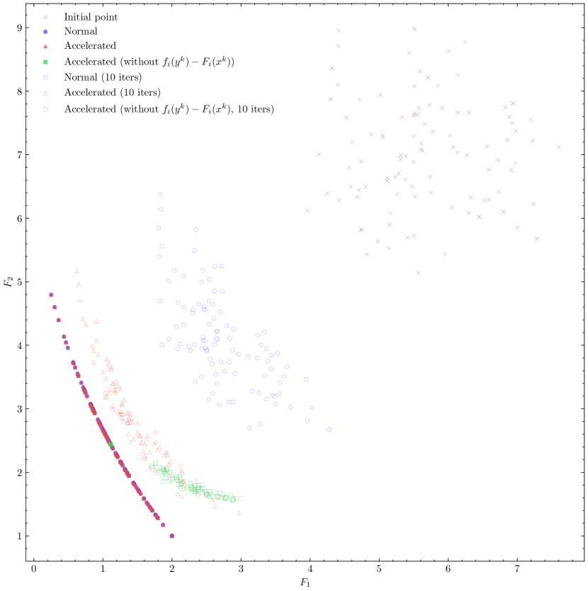
Figure 1: Objective function values for problem JOS1 with $n=50$, and $\ell_{1}$ norm for $g_{i}$

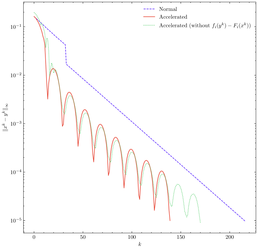
Figure 2: An example of $\left\{\left\lVert x^{k}-y^{k}\right\rVert_{\infty}\right\}$ for problem JOS1 with $n=50$, and $\ell_{1}$ norm for $g_{i}$

We now check the performance of the algorithms. As we explained in Section 7.2, for each problem of Table 1, we run the algorithms with $100$ different initial points. Table 2 shows the average of the computational time and iteration counts for each problem. For problems with different values of $n$, we just show the smallest and the biggest $n$ for convenience. From the table, it is possible to see that acceleration is in general more efficient in terms of time. In fact, by checking the performance profiles given in Figure 4 and Figure 4, we observe that our proposed Algorithm 2 performs better in terms of time and iteration counts. It is interesting to see from Table 2, however, that there are cases where Algorithm 2 does not perform well.

Table 2: Average computational costs

Problem	$n$	$g_{i}$	Total time (s)			Iteration counts
			Alg. 1	Alg. 2	Alg. 3	Alg. 1	Alg. 2	Alg. 3
JOS1	$5$	$0$	$0.032$	$0.029$	$0.027$	$23.82$	$27.89$	$27.89$
JOS1	$5$	$\ell_{1}$	$0.783$	$0.355$	$0.336$	$22.20$	$21.26$	$28.09$
JOS1	$1000$	$0$	$3.674$	$0.260$	$0.207$	$3203.05$	$155.00$	$155.00$
JOS1	$1000$	$\ell_{1}$	$183.957$	$47.913$	$46.197$	$2901.50$	$732.72$	$644.11$
ZDT1	$5$	ind.	$0.743$	$0.279$	$0.234$	$38.81$	$11.03$	$8.87$
ZDT1	$1000$	ind.	$1.738$	$0.840$	$0.634$	$32.68$	$14.30$	$9.986$
SD	$4$	ind.	$1.063$	$0.806$	$1.026$	$36.58$	$33.02$	$32.94$
TOI	$4$	$0$	$0.013$	$0.018$	$0.015$	$3.95$	$4.57$	$5.18$
TOI	$4$	$\ell_{1}$	$1.109$	$0.841$	$1.035$	$20.95$	$18.41$	$22.90$
TRIDIA	$3$	$0$	$94.447$	$0.981$	$5.842$	$3177.21$	$6.35$	$172.89$
TRIDIA	$3$	$\ell_{1}$	$79.562$	$3.892$	$78.616$	$1348.16$	$25.80$	$860.90$
FDS	$5$	$0$	$22.897$	$12.719$	$14.433$	$286.4$	$152.35$	$170.83$
FDS	$5$	$\ell_{1}$	$16.611$	$12.150$	$1330.424$	$127.48$	$91.39$	$13178.25$
FDS	$100$	$0$	$3805.058$	$4007.926$	$3607.842$	$644.45$	$117.27$	$158.72$
FDS	$100$	$\ell_{1}$	$4773.474$	$5412.802$	$5880.479$	$767.81$	$177.37$	$474.55$
LFR1	$30$	$0$	$4.904$	$8.335$	$4.362$	$9.18$	$11.67$	$6.69$
LFR1	$30$	$\ell_{1}$	$10.337$	$10.184$	$160.399$	$8.91$	$11.4$	$1224.37$
LFR1	$1000$	$0$	$10.928$	$13.804$	$10.916$	$8.54$	$10.07$	$8.36$
LFR1	$1000$	$\ell_{1}$	$26.669$	$31.038$	$26.566$	$8.55$	$10.31$	$8.56$

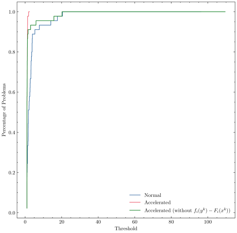
Figure 3: Performance profile:
computational time

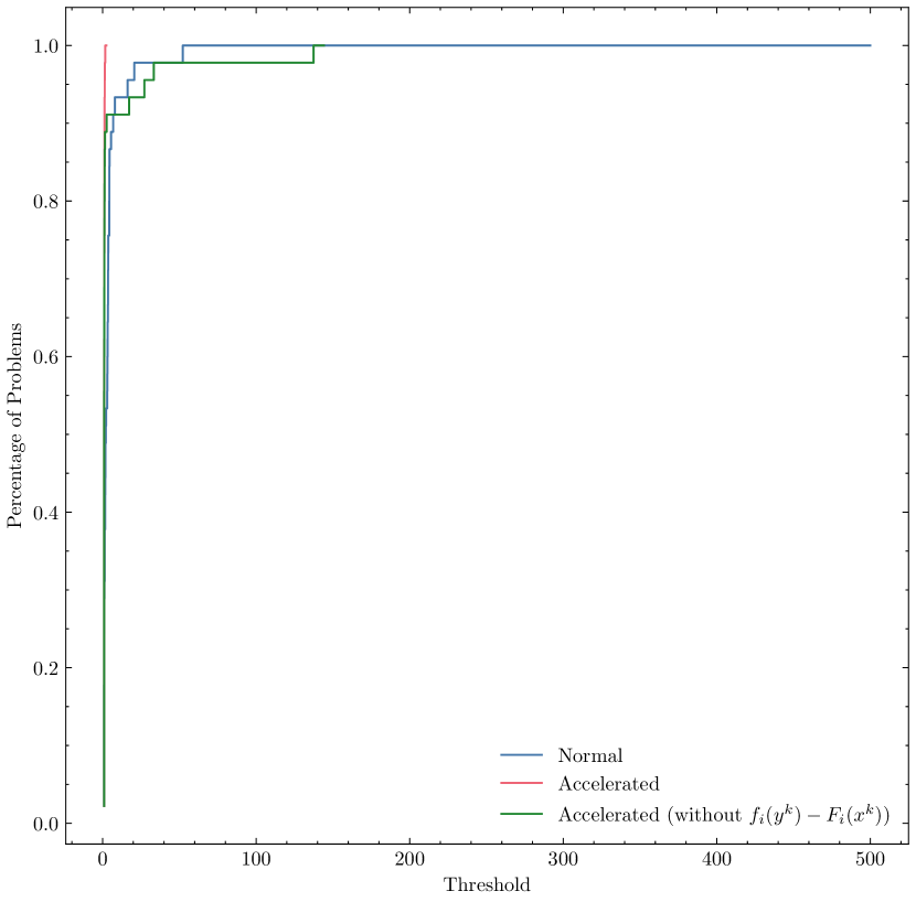
Figure 4: Performance profile:
iteration counts

Besides the performance, it is usually important to see how good the Pareto frontier is. Thus, once again we show performance profiles, this time for purity (Figure 6), hypervolume (Figure 6), spread metric $\Gamma$ (Figure 8) and spread metric $\Delta$ (Figure 8). Clearly, our proposed Algorithm 2 outperforms the other two algorithms, obtaining better Pareto frontiers. We can thus conclude that at least among the test problems considered, Algorithm 2 seem promising both in terms of performance and uniform Pareto frontiers.

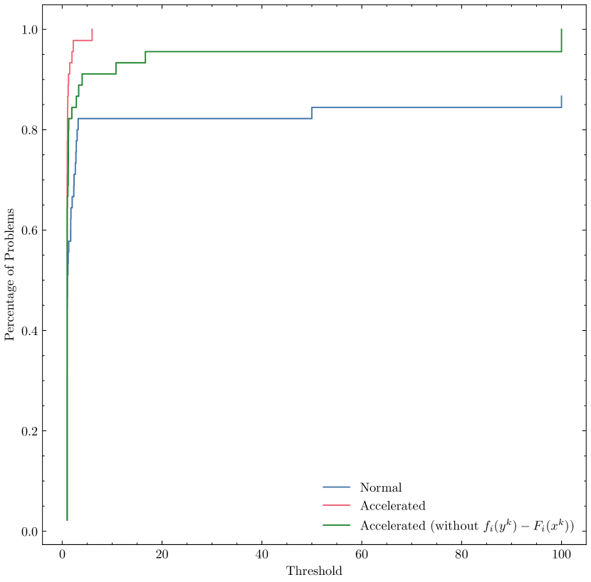
Figure 5: Performance profile:
purity

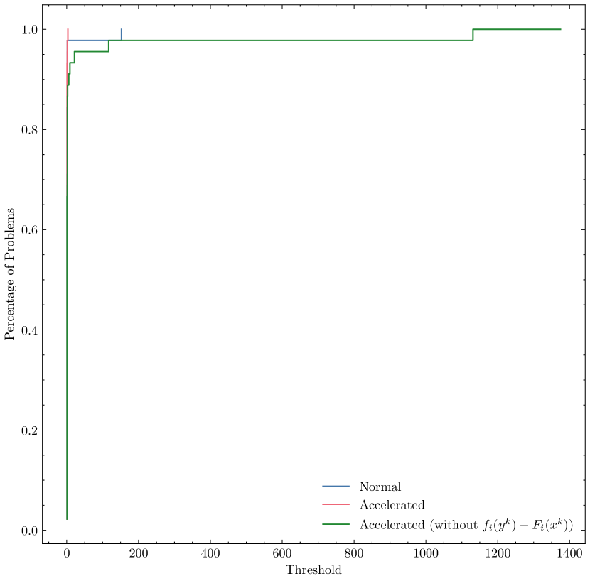
Figure 6: Performance profile: hypervolume

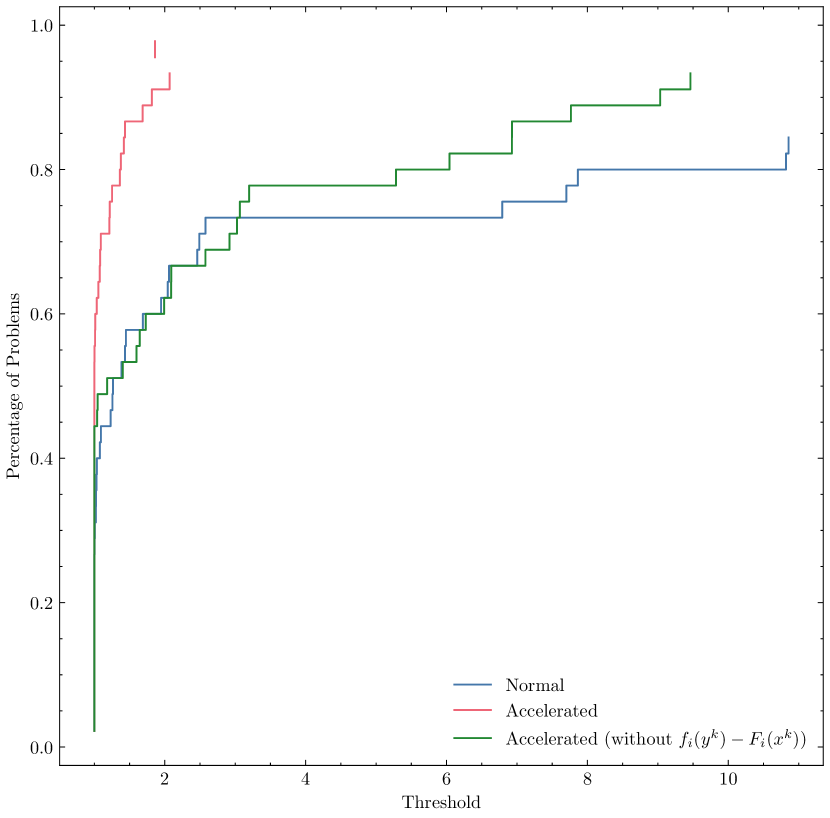
Figure 7: Performance profile:
spread metrics ($\Gamma$)

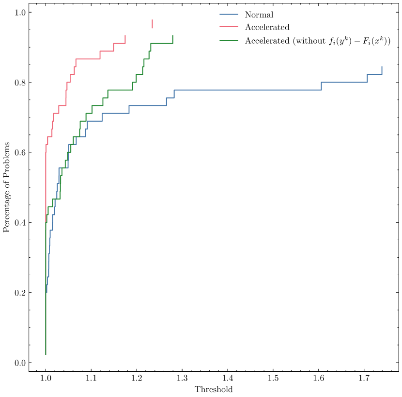
Figure 8: Performance profile:
spread metrics ($\Delta$)

8 Conclusion

By putting information of the previous points into the subproblem, we have successfully accelerated the proximal gradient method for multiobjective optimization and proved its convergence rate under natural assumptions, which was an open problem. Moreover, we showed an efficient way of computing the subproblem via its dual. As the experiments suggested, the proposed methods are also effective from the numerical point of view.

This paper shows the convergence rate for the sequence of the merit function values and the classical global convergence concerning accumulation points but does not provide the global convergence of the sequence of iterates itself. For single-objective optimization, by changing the update rule for the parameter $t_{k}$, Chambolle and Dossal have proposed a variant with the iterates’ global convergence [13]. In the multi-objective optimization problem, it may also be possible to modify the algorithm similarly and obtain the global convergence of iterates. Moreover, since many schemes for single-objective optimization had been developed, following the idea of Nesterov’s acceleration technique, this paper may also contribute to the development of various multiobjective optimization methods. Extensions to vector optimization and its generalization, the vector optimization problem with variable domination structure [8, 28], may also be worth considering. Such extensions will be subjects of future works.

References

• [1] Bandyopadhyay, S., Pal, S. and Aruna, B.: Multiobjective GAs, quantitative indices, and pattern classification, IEEE Transactions on Systems, Man and Cybernetics, Part B (Cybernetics), Vol. 34 (2004), 2088–2099.
• [2] Beck, A.: First-Order Methods in Optimization, Society for Industrial and Applied Mathematics, Philadelphia, Pennsylvania, USA, 2017.
• [3] Beck, A. and Teboulle, M.: A fast iterative shrinkage-thresholding algorithm for linear inverse problems, SIAM Journal on Imaging Sciences, Vol. 2 (2009), 183–202.
• [4] Bertsekas, D. P.: Nonlinear Programming, Athena Scientific, Belmont, Massachusetts, second edition, 1999.
• [5] Boţ, R. I. and Grad, S. M.: Inertial forward-backward methods for solving vector optimization problems, Optimization, Vol. 67 (2018), 959–974.
• [6] Bonnans, J. F. and Shapiro, A.: Perturbation Analysis of Optimization Problems, Springer New York, New York, NY, USA, 2000.
• [7] Bonnel, H., Iusem, A. N. and Svaiter, B. F.: Proximal methods in vector optimization, SIAM Journal on Optimization, Vol. 15 (2005), 953–970.
• [8] Bouza, G. and Tammer, C.: A steepest descent-like method for vector optimization problems with variable domination structure, Journal of Nonlinear and Variational Analysis, Vol. 6 (2022), 605–618.
• [9] Boyd, S. and Vandenberghe, L.: Convex Optimization, Cambridge University Press, Cambridge, England, 2004.
• [10] Brent, R. P.: Algorithms for Minimization without Derivatives, Prentice-Hall, New Jersey, 1973.
• [11] Byrd, R. H., Hribar, M. E. and Nocedal, J.: An interior point algorithm for large-scale nonlinear programming, SIAM Journal on Optimization, Vol. 9 (1999), 877–900.
• [12] Carrizo, G. A., Lotito, P. A. and Maciel, M. C.: Trust region globalization strategy for the nonconvex unconstrained multiobjective optimization problem, Mathematical Programming, Vol. 159 (2016), 339–369.
• [13] Chambolle, A. and Dossal, C.: On the convergence of the iterates of the “Fast Iterative Shrinkage/Thresholding Algorithm”, Journal of Optimization Theory and Applications, Vol. 166 (2015), 968–982.
• [14] Custódio, A. L., Madeira, J. F., Vaz, A. I. and Vicente, L. N.: Direct multisearch for multiobjective optimization, SIAM Journal on Optimization, Vol. 21 (2011), 1109–1140.
• [15] Dolan, E. D. and Moré, J. J.: Benchmarking optimization software with performance profiles, Mathematical Programming, Series B, Vol. 91 (2002), 201–213.
• [16] El Moudden, M. and El Mouatasim, A.: Accelerated diagonal steepest descent method for unconstrained multiobjective optimization, Journal of Optimization Theory and Applications, Vol. 188 (2021), 220–242.
• [17] Fliege, J., Graña Drummond, L. M. and Svaiter, B. F.: Newton’s method for multiobjective optimization, SIAM Journal on Optimization, Vol. 20 (2009), 602–626.
• [18] Fliege, J. and Svaiter, B. F.: Steepest descent methods for multicriteria optimization, Mathematical Methods of Operations Research, Vol. 51 (2000), 479–494.
• [19] Fliege, J., Vaz, A. I. F. and Vicente, L. N.: Complexity of gradient descent for multiobjective optimization, Optimization Methods and Software, Vol. 34 (2019), 949–959.
• [20] Fukuda, E. H. and Graña Drummond, L. M.: Inexact projected gradient method for vector optimization, Computational Optimization and Applications, Vol. 54 (2013), 473–493.
• [21] Fukuda, E. H. and Graña Drummond, L. M.: A survey on multiobjective descemt methods, Pesquisa Operacional, Vol. 34 (2014), 585–620.
• [22] Gandibleux, X., Sevaux, M., Sörensen, K. and T’kindt, V.: Metaheuristics for Multiobjective Optimisation, Vol. 535 of Lecture Notes in Economics and Mathematical Systems, Springer Berlin Heidelberg, Berlin, Heidelberg, 2004.
• [23] Gass, S. and Saaty, T.: The computational algorithm for the parametric objective function, Naval Research Logistics Quarterly, Vol. 2 (1955), 39–45.
• [24] Geoffrion, A. M.: Proper efficiency and the theory of vector maximization, Journal of Mathematical Analysis and Applications, Vol. 22 (1968), 618–630.
• [25] Gonçalves, M. L. N., Lima, F. S. and Prudente, L. F.: Globally convergent Newton-type methods for multiobjective optimization, Computational Optimization and Applications, Vol. 83 (2022), 403–434.
• [26] Graña Drummond, L. M. and Iusem, A. N.: A projected gradient method for vector optimization problems, Computational Optimization and Applications, Vol. 28 (2004), 5–29.
• [27] Jin, Y., Olhofer, M. and Sendhoff, B.: Dynamic weighted aggregation for evolutionary multi-objective optimization: Why does it work and how?, in Proceedings of the 3rd Annual Conference on Genetic and Evolutionary Computation, GECCO’01, San Francisco, CA, USA, 2001, Morgan Kaufmann Publishers Inc.
• [28] Köbis, E., Köbis, M. A. and Tammer, C.: A first bibliography on set and vector optimization problems with respect to variable domination structures, Journal of Nonlinear and Variational Analysis, Vol. 6 (2022), 725–735.
• [29] Lucambio Pérez, L. R. and Prudente, L. F.: Nonlinear conjugate gradient methods for vector optimization, SIAM Journal on Optimization, Vol. 28 (2018), 2690–2720.
• [30] Marler, R. T. and Arora, J. S.: The weighted sum method for multi-objective optimization: New insights, Structural and Multidisciplinary Optimization, Vol. 41 (2010), 853–862.
• [31] Mita, K., Fukuda, E. H. and Yamashita, N.: Nonmonotone line searches for unconstrained multiobjective optimization problems, Journal of Global Optimization, Vol. 75 (2019), 63–90.
• [32] Moré, J. J., Garbow, B. S. and Hillstrom, K. E.: Testing unconstrained optimization software, ACM Transactions on Mathematical Software, Vol. 7 (1981), 17–41.
• [33] Moreau, J.-J.: Proximité et dualité dans un espace hilbertien, Bulletin de la Société Mathématique de France, Vol. 93 (1965), 273–299.
• [34] Nesterov, Y.: A method for solving the convex programming problem with convergence rate $O(1/k^{2})$, Doklady Akademii Nauk SSSR, Vol. 269 (1983), 543–547.
• [35] Parikh, N. and Boyd, S.: Proximal Algorithms, Vol. 1, Now Publishers, Inc., Boston - Delft, 2014.
• [36] Rockafellar, R. T. and Wets, R. J. B.: Variational Analysis, Vol. 317 of Grundlehren der mathematischen Wissenschaften, Springer Berlin Heidelberg, Berlin, Heidelberg, 1998.
• [37] Sion, M.: On general minimax theorems, Pacific Journal of Mathematics, Vol. 8 (1958), 171–176.
• [38] Stadler, W. and Dauer, J.: Multicriteria optimization in engineering: a tutorial and survey, in Kamat, M. P. ed., Progress in Aeronautics and Astronautics: Structural Optimization: Status and Promise, Vol. 150, Washington DC, 1992, American Institute of Aeronautics and Astronautics.
• [39] Svaiter, B. F.: The multiobjective steepest descent direction is not Lipschitz continuous, but is Hölder continuous, Operations Research Letters, Vol. 46 (2018), 430–433.
• [40] Tanabe, H., Fukuda, E. H. and Yamashita, N.: Proximal gradient methods for multiobjective optimization and their applications, Computational Optimization and Applications, Vol. 72 (2019), 339–361.
• [41] Tanabe, H., Fukuda, E. H. and Yamashita, N.: Convergence rates analysis of a multiobjective proximal gradient method, Optimization Letters, Vol. 17 (2023), 333–350.
• [42] Tanabe, H., Fukuda, E. H. and Yamashita, N.: New merit functions for multiobjective optimization and their properties, arXiv:2010.09333, 2023.
• [43] Toint, P. L.: Test problems for partially separable optimization and results for the routine PSPMIN, Namur Report, 1983.
• [44] Wang, X., Wang, Y. and Wang, G.: An accelerated augmented lagrangian method for multi-criteria optimization problem, Journal of Industrial and Management Optimization, Vol. 16 (2020), 1–9.
• [45] Yosida, K.: Functional Analysis, Vol. 123 of Classics in Mathematics, Springer Berlin Heidelberg, Berlin, Heidelberg, sixth edition, 1995.
• [46] Zadeh, L. A.: Optimality and non-scalar-valued performance criteria, IEEE Transactions on Automatic Control, Vol. 8 (1963), 59–60.
• [47] Zhao, X., Jolaoso, L. O., Shehu, Y. and Yao, J.-C.: Convergence of a nonmonotone projected gradient method for nonconvex multiobjective optimization, Journal of Nonlinear and Variational Analysis, Vol. 5 (2021), 441–457.
• [48] Zitzler, E., Deb, K. and Thiele, L.: Comparison of multiobjective evolutionary algorithms: empirical results, Evolutionary Computation, Vol. 8 (2000), 173–195.
• [49] Zitzler, E., Technische, E. and Zürich, H.: Evolutionary Algorithms for Multiobjective Optimization: Methods and Applications, Phd thesis, Swiss Federal Institute of Technology Zurich, 1999.
• [50] Zou, H. and Hastie, T.: Regularization and variable selection via the elastic net, Journal of the Royal Statistical Society: Series B (Statistical Methodology), Vol. 67 (2005), 301–320.