Applying Grover’s Algorithm to Hash Functions:
A Software Perspective

Abstract

Quantum software frameworks provide software engineers with the tools to study quantum algorithms as applied to practical problems. We implement classical hash functions MD5, SHA-1, SHA-2, and SHA-3 as quantum oracles to study the computational resource requirements of conducting a preimage attack with Grover’s Algorithm. We introduce an improvement to the SHA-3 oracle that reduces the number of logical qubits required in the Keccak block permutation by 40%.

1 Introduction

Consider the following scenario. On a certain banking website, customers log in by entering their username and password. Before being sent to the server for authentication, the password is salted (random data is appended) and then passed through a cryptographic hash function.

Suppose an attacker gains access to the plaintext hash and salt. With conventional (classical) computers, the only way to recover the original password is with guess-and-check, a.k.a. brute-force. Assuming an 8-character password consisting of random characters, the attacker would have to check approximately $2^{64}=1.8\times 10^{19}$ combinations. At a rate of 1 billion checks per second, it would take on-average 292 years to find the password, at which point it is probably useless.

But what if the attacker had access to a powerful quantum computer? With Grover’s Algorithm, the password could be found directly in $\sqrt{2^{64}}=4.3\times 10^{9}$ iterations [1]. Assuming the same rate of 1 billion iterations per second, this could be accomplished in a matter of seconds. The attacker could then log in and steal the customer’s funds before the breach is detected. Fortunately in this scenario, today’s quantum computers are not capable of performing computations of this scale. However, it is critically important to understand precisely what computational resources would be required for such an attack.

The objective of this research was to study the computational cost of conducting a preimage attack on MD5, SHA-1, SHA-2, and SHA-3 with Grover’s Algorithm. We used Microsoft’s Quantum Development Kit (QDK) to implement each hash function as a quantum oracle, validate the implementations through simulation, and then estimate the quantum hardware requirements to apply Grover’s Algorithm.

1.1 Background

Grover’s Algorithm can reverse a black-box function implemented as a quantum oracle in $\mathrm{O}(\sqrt{N})$ iterations with $\mathrm{O}(\log_{2}{N})$ qubits, with $N$ being the number of possible input combinations to the function [1]. In this context, the quantum oracle phase-flips a target qubit when the desired output is produced (e.g., when the password is correct). Grover’s Algorithm searches for the input(s) that cause the phase-flip to occur.

The steps of the algorithm are given below. Assume $n$ is the number of input bits, $N=2^{n}$, and $k$ is the number of “correct” input combinations or search targets.

1. Allocate $n$ input qubits and 1 target qubit.

   $$\ket{\mathrm{I},\mathrm{T}}=\ket{0^{\otimes n},0}$$

2. Apply H to each input qubit.

   $$\ket{\mathrm{I},\mathrm{T}}=\frac{1}{\sqrt{N}}\sum_{i=0}^{N-1}\ket{i}\otimes\ket{0}$$

3. Apply X to the target qubit.

   $$\ket{\mathrm{I},\mathrm{T}}=\frac{1}{\sqrt{N}}\sum_{i=0}^{N-1}\ket{i}\otimes\ket{1}$$

4. Do the following $\left\lfloor\frac{\pi}{4}\sqrt{\frac{N}{k}}\right\rfloor$ times:

   1. Apply the oracle.

   2. Apply H to each input qubit.

   3. Apply Z to the target qubit, zero-controlled on all input qubits.

   4. Apply H to each input qubit.

5. Measure the input qubits. The result will be a value that produces the desired output with probability approaching 1 for large $N$. Check the outcome and repeat if the search failed.

Fig. 1 shows the circuit diagram for Grover’s Algorithm. Note how the oracle is constructed such that any operations applied in computing the black-box function are reversed.

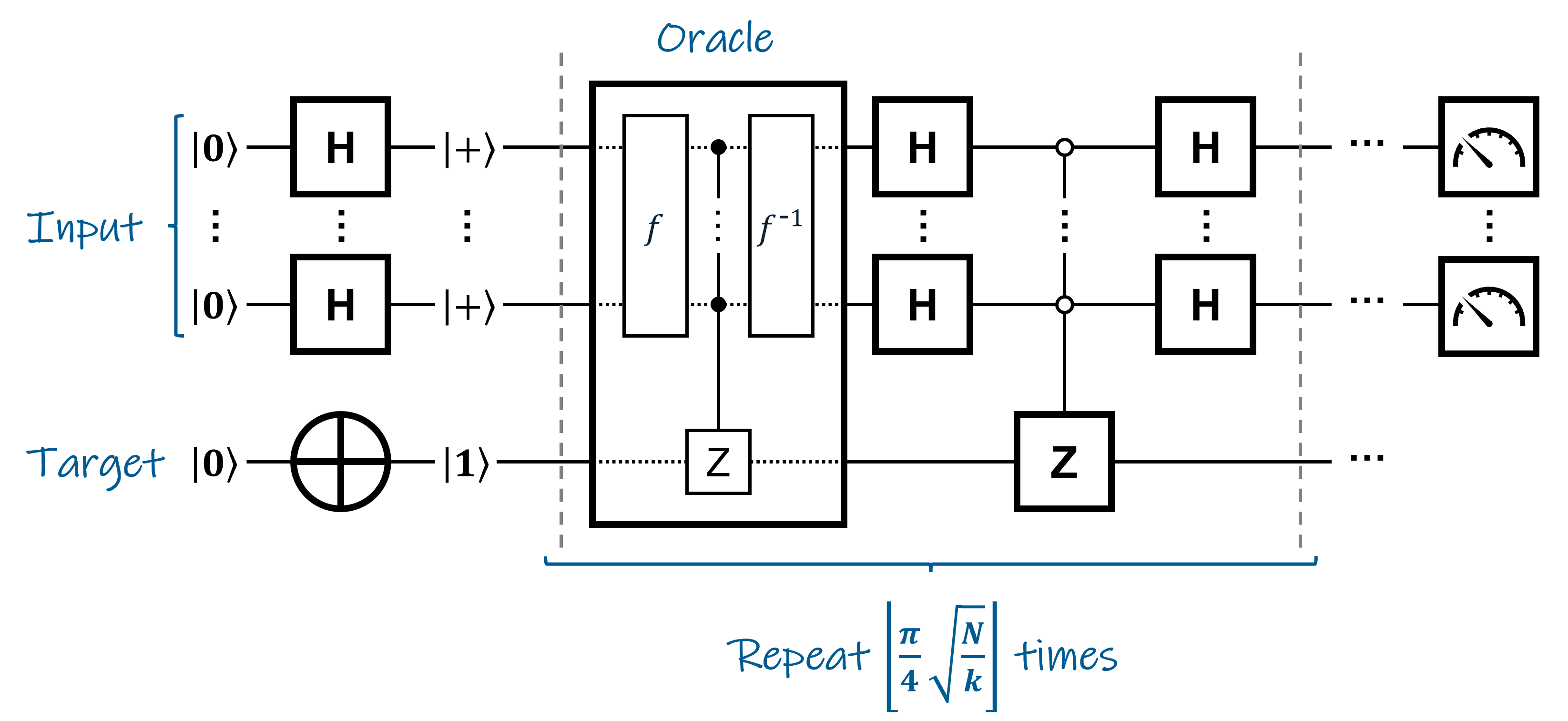
Figure 1: Grover’s Algorithm

The challenge in applying Grover’s Algorithm to a hash function lies in translating the classical algorithm into a quantum one. Referring again to Fig. 1, the $f$ and $f^{-1}$ in the oracle are not given – they must be designed using quantum computing primitives. Section 2 details how MD5, SHA-1, SHA-2, and SHA-3 can be translated into quantum oracles so the quantum preimage attack can be conducted.

1.2 Related Work

The most relevant paper to this work is “Estimating the cost of generic quantum pre-image attacks on SHA-2 and SHA-3” (2016), where Amy et al. analyze the computational resources required to run Grover’s Algorithm on SHA-256 and SHA3-256, assuming a surface code based quantum computer [2]. They provide oracle implementations for the hash functions and make precise, educated estimates on the number of logical qubits and surface code cycles that would be needed. There are three important ways in which our work differs from theirs:

1. Our analysis includes the entire SHA-2 and SHA-3 families, as well as MD5 and SHA-1.

2. We fully implement the preimage attack as a quantum software program and use a resource estimator to generate the cost metrics. This approach has benefits and limitations, as discussed in Section 5.

3. We introduce an improvement to the SHA-3 implementation that reduces the number of logical qubits required.

Our research is an example of a “practicality assessment” of a quantum computing application. Rather than introduce a novel quantum algorithm, a practicality assessment seeks to precisely understand the computational requirements of applying an existing algorithm, with all the implementation details laid bare. A similar approach is taken by Joe Clapis in his report, “A Quantum Dot Plot Generation Algorithm for Pairwise Sequence Alignment” [3]. In that work, he finds that the Quantum Pairwise Sequence Alignment algorithm proposed by Prousalis and Konfaos [4] relies on a black-box operation that overwhelms the rest of the algorithm in terms of computational complexity when a practical implementation is attempted. Such insights are critical as quantum computers become advanced enough to solve real-world problems.

2 Approach

The entirety of this work was conducted using Microsoft’s QDK, with the majority of the code written in Q#, Microsoft’s programming language for quantum computing [5]. The QDK provides built-in simulation and estimation capabilities that allowed us to validate the correctness of the program before obtaining resource requirement metrics. Of particular use was the Toffoli simulator, which can simulate large numbers of qubits but only allows X and controlled X gates. (It essentially treats the qubits as classical bits.) This allowed us to fully test any operation that was derived from a classical function.

The procedure we followed consists of three steps:

1. Implement the hash function as a quantum operation in Q#.

2. Validate the correctness of the program using the Toffoli simulator.

3. Estimate the computational resources required to conduct a preimage attack with Grover’s Algorithm.

The first step is the most challenging, since quantum and classical computing occupy two completely different paradigms. It is oftentimes inefficient or even impossible to translate a classical function directly into a quantum one. For example, since measurement destroys superposition, you cannot “set” or “clear” a qubit like you can a classical bit. This is particularly relevant in managing working memory because any operations performed on temporary qubits must be reversed before they can be reused; you can’t just set them to zero directly. You also cannot create an independent copy of a qubit (no-cloning theorem [6]), something that is trivial and highly useful in classical programming.

The remainder of this section describes each hash function studied and highlights the key differences in their classical and quantum implementations.

2.1 MD5

The high-level designs of MD5, SHA-1, and SHA-2 are very similar to each other. They are all built using a Merkle–Damgård construction, and therefore contain the following elements [7][8]:

• The input message is padded using a special function that extends its length to be a multiple of a certain number (e.g. 512). A property of the padding function is that it encodes the original input length.

• The message is broken up into fixed-length blocks or chunks that are processed one at a time.

• The chunks are processed with a one-way compression function that mixes two fixed-length inputs into an output of length equal to one of the inputs. Specifically, each chunk is mixed with the output of processing the previous chunk. (There is an initialization vector to mix with the first chunk.)

In the case of MD5, SHA-1, and SHA-2, the compression functions are composed of computational iterations that include nonlinear Boolean functions, arithmetic addition, and bitwise rotation. They all follow the same basic pattern but differ in the specific operations employed. In MD5, there is a 128-bit state that is initialized to a fixed value and updated after each chunk is processed. The compression function applied to the chunks consists of 64 iterations that transform a copy of the 128-bit state broken into four 32-bit working registers, $a$, $b$, $c$, and $d$. After the iterations are complete, the registers are recombined, and the result is added to the original state before proceeding to the next chunk.

Fig. 2 illustrates the computation involved in a single MD5 iteration. In the diagram, the plus sign means arithmetic addition and the clockwise arrow means bitwise left-rotate. $W_{i}$ is a 32-bit word in the message block determined by the iteration index. $K_{i}$ and $s_{i}$ are predetermined constants. $F_{i}$ is one of four nonlinear Boolean functions that are each used for 16 of the 64 iterations per chunk. All values are modulus 32-bit and little-endian. Note how the names of the working registers are shuffled after each iteration. See IETF RFC 1321 for the full MD5 specification [9].

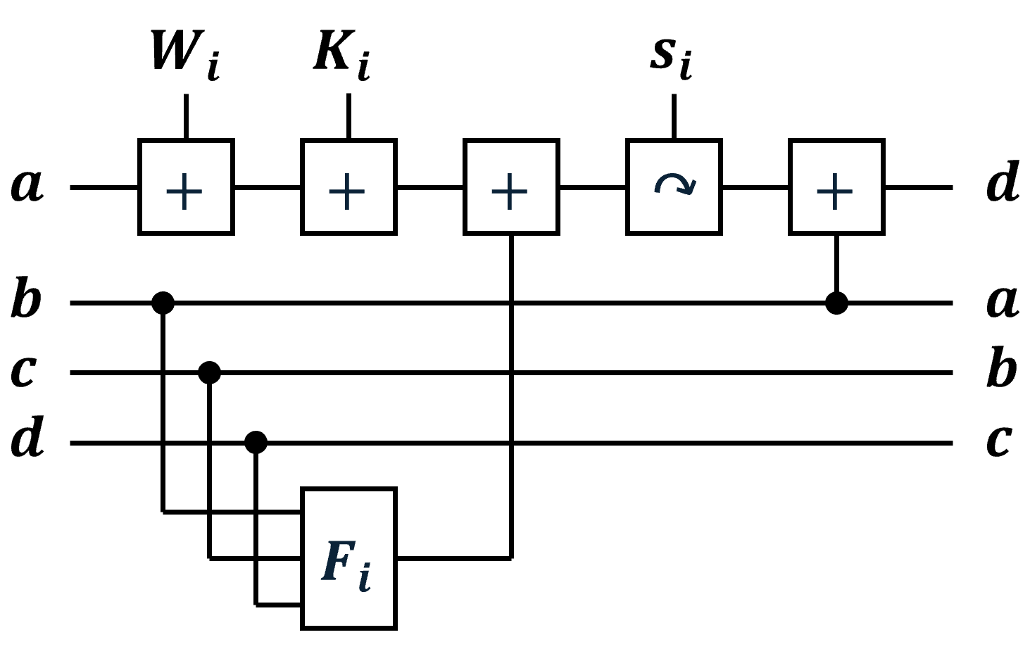
Figure 2: Single MD5 Iteration

The main considerations when creating a quantum version of a classical algorithm are (1) how the individual operations translate, (2) how to minimize the number of qubits required, and (3) how to ensure that the entire design is reversible, i.e., it supports the adjoint functor in Q#. For example, MD5 uses many arithmetic additions. Q# offers a library function implementing an in-place quantum ripple carry adder, which can be used to handle addition between two qubit registers. However, this cannot be used to add a constant ($K_{i}$) directly. Instead, it must first be encoded in a temporary qubit register using an in-place XOR, and then added normally. Once the addition is done, the temporary register must be returned to zero by applying the XOR again so the qubits can be de-allocated. This entire process is reversible, so it can be used in the overall design.

Fig. 3 shows the strategy we employed for implementing MD5 in quantum software. Here, all values are little-endian encoded in 32-qubit registers. The plus sign means in-place arithmetic addition of two qubit registers. The clockwise arrow is a re-indexing of the qubit register which has the effect of a bitwise left-rotate. $W_{i}$ is a 32-qubit segment of the message block determined by the iteration index. $K_{i}$ and $s_{i}$ are the same as before. Quantum versions of $F_{i}$ perform the Boolean functions in-place, so that the output is stored in $c$ or $d$. $F_{i}$ is reversed after the result is added to $a$ to preserve the contents of the working registers.

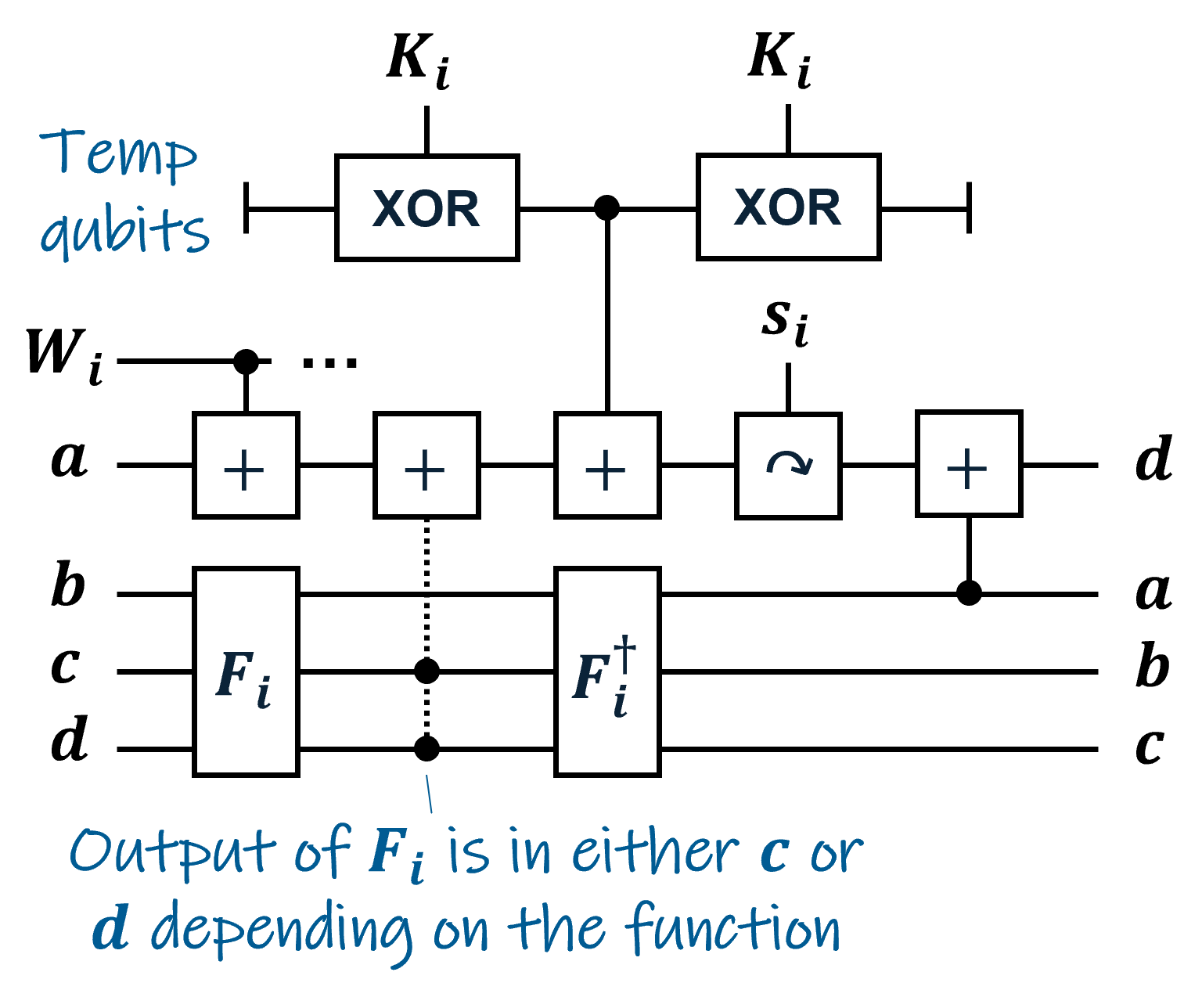
Figure 3: Quantum Version of MD5 Iteration

One complication of the quantum implementation of MD5 is that, classically, the working registers are reset after each chunk is processed and their contents are added to the state. This would prevent Grover’s algorithm from being applied because (1) directly resetting a qubit involves measuring it, which would destroy any superposition, and (2) the contents of the working registers are needed for the entire design to be reversible. Thus, 128 workspace qubits are needed per chunk if the adjoint functor is to be supported. This is not so surprising when considering that hash algorithms are designed to be one-way, and so additional state information is needed to reverse them directly. That is, you (obviously) cannot directly reverse a hash algorithm given only the output – otherwise that would defeat the entire purpose!

2.2 SHA-1

SHA-1 is very similar in structure to MD5, except the state is 160 bits instead of 128, so it uses five 32-bit working registers when processing each chunk. Also, each chunk is extended to 2560 bits (eighty 32-bit words) by mixing the original message block in a deterministic fashion. The SHA-1 compression function uses 80 iterations instead of 64, where a single iteration is as illustrated by Fig. 4. See IETF RFC 3174 for the full specification of SHA-1 [11].

The Boolean functions and constants are distinct from MD5, but the general pattern is the same. The working registers are shuffled in a different order, with the additions performed on $e$ instead of $a$. Register $b$ is also bitwise left-rotated by 10 each iteration.

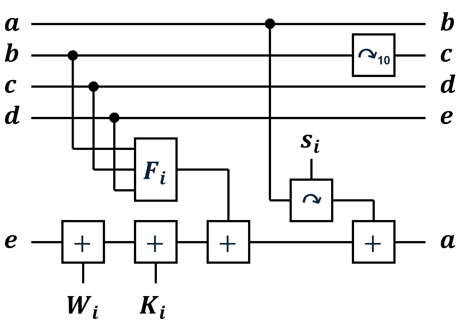
Figure 4: Single SHA-1 Iteration

Fig. 5 shows how we implemented a SHA-1 iteration with similar strategies to MD5. Just as before, each horizontal line represents a little-endian value encoded in a 32-qubit register. (Note that the left-rotated version of $a$ added to $e$ does not count as additional qubits since it is just a re-indexing of the register.) Thus, 160 qubits are required for the working registers, plus 32 temporary qubits to add the constant $K_{i}$ to $e$. $W_{i}$ comes from the 80-word message schedule generated from the message block before the iterations begin. We again have the unfortunate situation that the 160 workspace qubits must be preserved after each chunk is processed to make the entire design reversible.

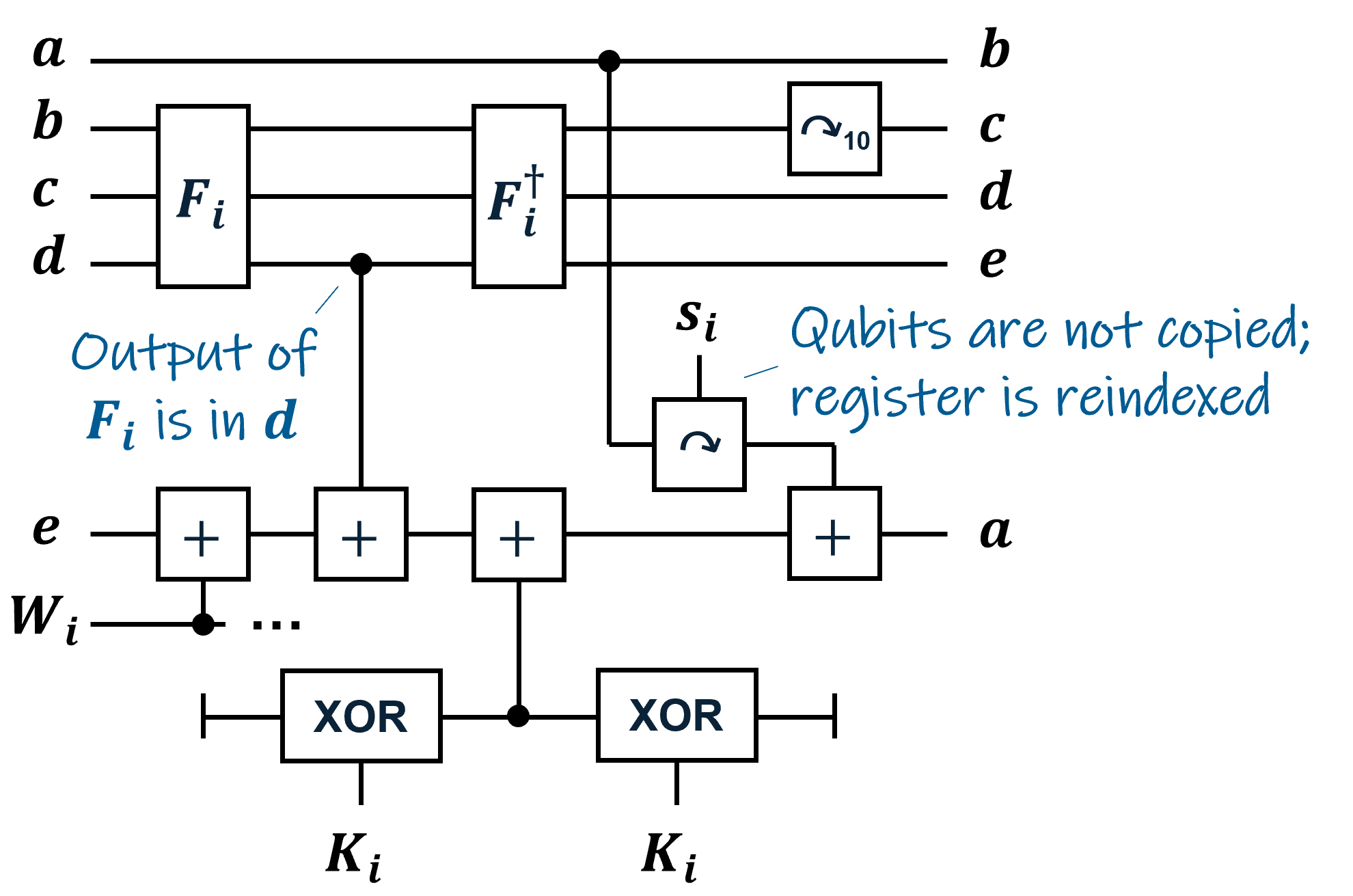
Figure 5: Quantum Version of SHA-1 Iteration

2.3 SHA-2

SHA-2 is the latest hash algorithm standard utilizing a Merkle–Damgård construction. The NIST specification lists six functions that vary in strength and output size: SHA-224, SHA-256, SHA-384, SHA-512, SHA-512/224, and SHA-512/256 [12]. The important difference between these is that SHA-224 and SHA-256 uses 32-bit words and 512-bit chunks, while the others use 64-bit words and 1024-bit chunks. The state consists of eight words, so it’s either 256 or 512 bits depending on the word length. The compression function performs 64 iterations on eight working registers as shown in Fig. 6.

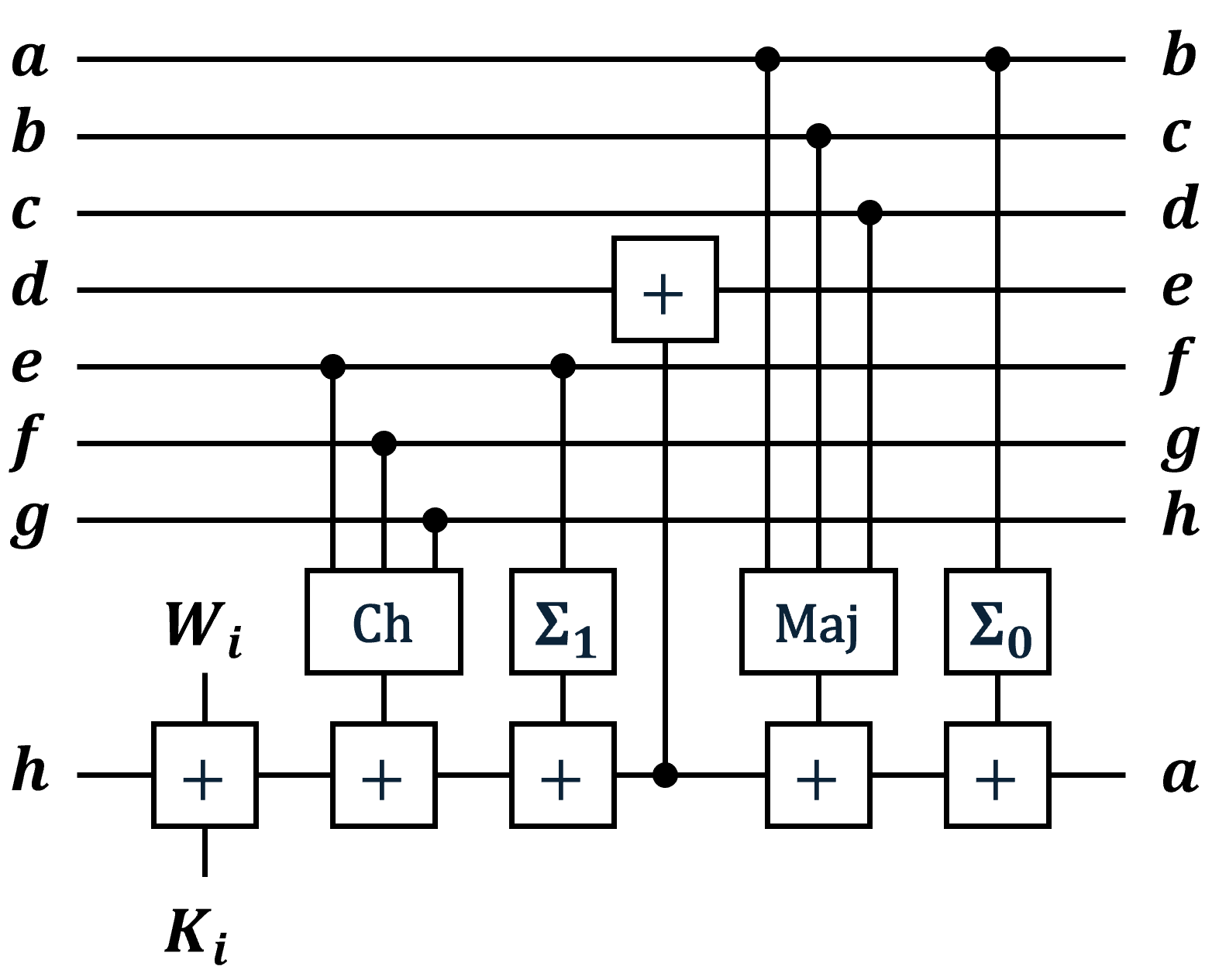
Figure 6: Single SHA-2 Iteration

Here, $W_{i}$ again comes from a message schedule generated by extending the 16-word chunk into 64 words. (The steps to generate the message schedule are slightly more complex than SHA-1, but the effect is similar.) “Ch” is short for bitwise choice. In this case, each bit of the output follows $f$ if $e$ is 1, and $g$ if $e$ is 0. “Maj” is short for bitwise majority, where each bit of the output follows whatever value occurs most frequently on the inputs. $\Sigma_{1}$ and $\Sigma_{0}$ involve XORing together bitwise rotated copies of the input. Note an intermediate value is added to $d$ partway through the iteration.

SHA-2 is a little tricker to implement in quantum software because all these functions must be performed in-place and then reversed, as shown in Fig. 7. The main thing to notice in the figure is the use of temporary qubits for the $\Sigma$ functions. This is because they cannot be computed in-place and so a register is needed to store the result. Fortunately, the same qubits can be recycled for constant addition and both $\Sigma$ functions, so only one extra word is needed.

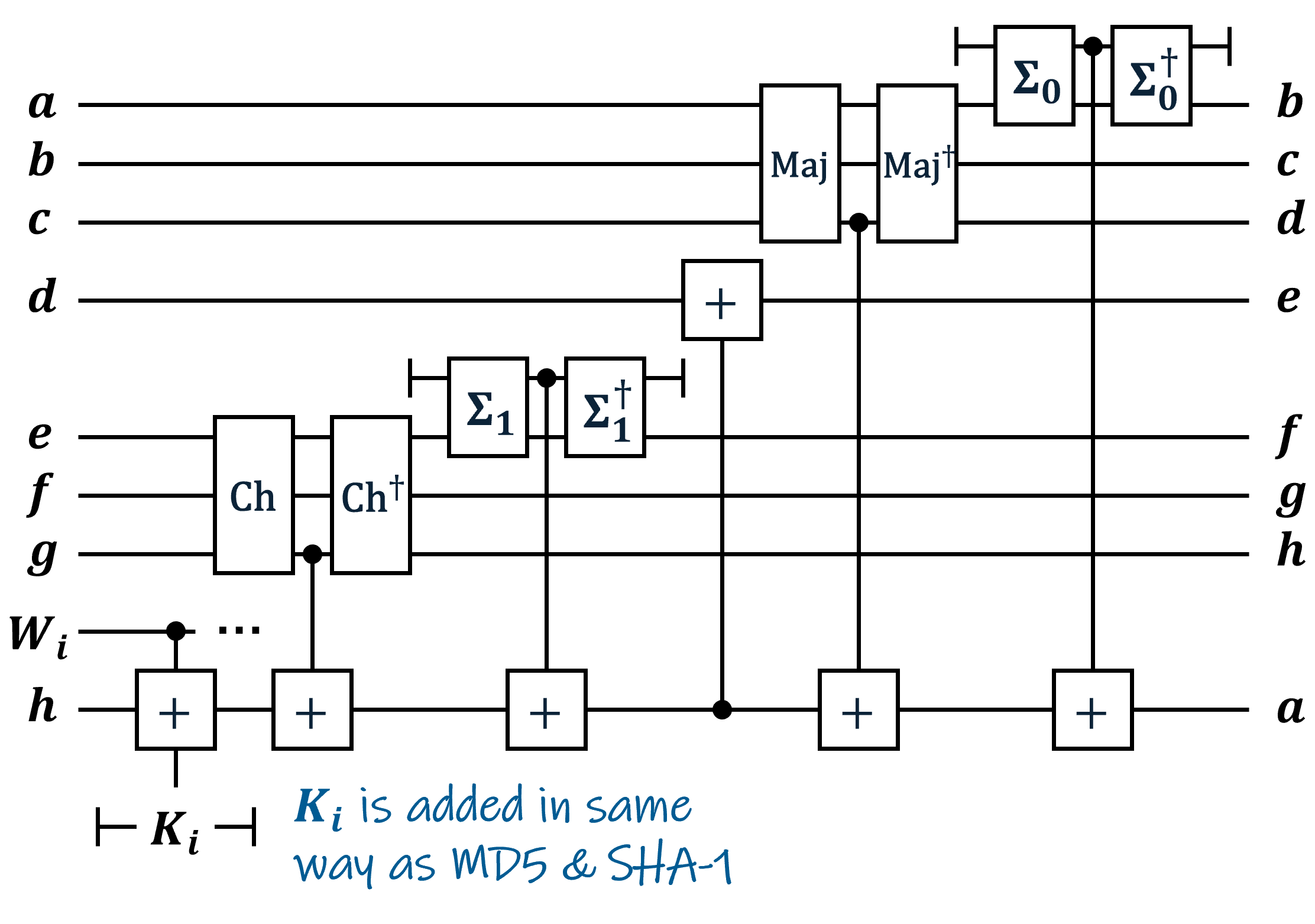
Figure 7: Single SHA-2 Iteration

Architecturally, the Merkle–Damgård-based functions lend themselves well to quantum implementation. However, the addition operation prevalent throughout these is relatively expensive in computational cost. (In contrast to a classical computer, there is no dedicated ALU to perform the addition; each plus block represents a string of quantum gates implementing a ripple-carry adder.) The situation is opposite for SHA-3 – the hash function is architecturally complex and difficult to implement, but it does not rely on arithmetic addition.

2.4 SHA-3

SHA-3 was designed to be an effective, unique alternative to provide resiliency in the case of a catastrophic vulnerability being discovered in SHA-2. It is based on a cryptographic primitive called Keccak, which utilizes a sponge construction to process the input message and generate the output digest [13]. The high-level steps of Keccak are:

1. Pad the input message so its length is divisible by a fixed value $r$ (the bitrate) and the final byte is a specified suffix.

2. Break the input into chunks of length $r$.

3. Allocate a state register initialized to all zeros (for SHA-3 this is 1600 bits).

4. “Absorb” phase. For each chunk:

   1. XOR the chunk with the first $r$ bits of the state.

   2. Apply a complex function to the state called the block permutation.

5. “Squeeze” phase. While more output is desired:

   1. Append the first $r$ bits of the state to the output.

   2. Apply the block permutation.

The SHA-3 NIST specification defines drop-in replacements for SHA-2 functions with the same level of security: SHA3-224, SHA3-256, SHA3-384, and SHA3-512 [14]. It also introduces two functions with variable-length output, SHAKE128 and SHAKE256. These all follow the above steps, but with different values for the padding suffix and bitrate. (Note that a lower bitrate or $r$ value means a higher level of security since it results in more permutations.)

For SHA-3, the devil is in the details of the block permutation. First, the 1600-bit state register is mapped to a 5x5x64 array, and then five functions are applied in succession: $\theta$, $\rho$, $\pi$, $\chi$, and $\iota$. These are composed of only XOR, AND, and NOT gates, plus permutations of the bits in the array, so they are relatively straightforward to implement on a classical computer. Importantly, they are all invertible, i.e., for each function, another function exists that maps the output of the original to the corresponding input, for all such input/output pairs. This is not just theoretical – the Keccak authors provide C++ implementations of the inverse functions in the KeccakTools GitHub repository.

Amy et al. showed how the block permutation could be performed in-place on a quantum computer [2]. Since $\rho$ and $\pi$ only consist of permutations or rotations, they could be implemented by reordering the state array (no quantum gates required). And $\iota$ simply XORs the first lane of the state array with a constant that depends on the round, which we have seen before. However, $\theta$ and $\chi$ are trickier; the former involves computing the parities of each column in the state array, and the latter is a non-linear function utilizing AND and NOT. Amy et al. mapped the classical steps of these functions directly to quantum gates, so that the output would be constructed in a new 1600-qubit register. Then, they applied the inverse function with the input/output registers swapped, transforming the original input register to all $\ket{0}$’s so those qubits could be released (de-allocated). Fig. 8 illustrates the authors’ strategy for computing the Keccak block permutation in-place in a quantum context.

Figure 8: In-Place Keccak Block Permutation Using Inverse Functions

While the entire block permutation is computed in-place with the above approach, $\theta$ and $\chi$ individually are not. That is, the two functions store the result in an output register, rather than modifying the input register. When implementing these in Q#, it was discovered that $\theta$ and $\chi$ could themselves be computed in-place, requiring fewer qubits and gates than allocating an output register and computing the inverse. For both functions, a working memory of 320 qubits is used to store intermediate values necessary to transform the input, and then a modified version of the inverse function is used to recompute those intermediate values so the ancillary qubits can be released. This modified inverse is denoted by $\theta^{-1^{\prime}}$ in Fig 9; the modified inverse for $\chi$ is not shown. Using the method below, the block permutation can be performed with only 1920 logical qubits, instead of the 3200 required by Amy’s approach, without increasing the gate depth.

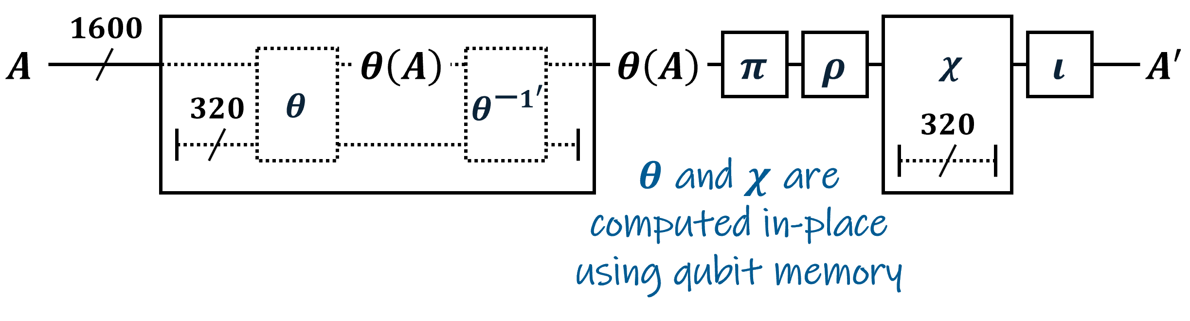
Figure 9: Qubit-Efficient Keccak Block Permutation

Listing 1 shows the Q# implementation of the in-place theta function. Note that the modified inverse is built-in so that the ancilla qubits can be scoped to the single operation (they are allocated and de-allocated within it). The code is based on the Keccak team’s classical implementation of the inverse theta function, and uses the following custom operations:

• ArrayAsWords: Breaks up a flat array into an array of words with specified length.

• Xor: Applies CNOT to each pair of qubits in the parallel array arguments.

• RightRotate: Shifts an array to the right in a circular manner by a specified amount. I.e., elements that “fall off” the right are “fed into” the left.

Listing 1: In-Place Theta Function

⬇

operation Theta (lanes : Qubit[][][]) : Unit

is Adj + Ctl {

use temp = Qubit[320];

// Compute column parities

let cols = ArrayAsWords(64, temp);

for x in 0 .. 4 {

for y in 0 .. 4 {

Xor(lanes[(x+4) % 5][y], cols[x]);

Xor(

RightRotate(lanes[(x+1) % 5][y], 1),

cols[x]

);

}

}

// Xor parities into the state array

for x in 0 ..4 {

for y in 0 .. 4 {

Xor(cols[x], lanes[x][y]);

}

}

// Return temp qubits to |0>

let inversePositions = [

0xDE26BC4D789AF134L,

0x09AF135E26BC4D78L,

0xEBC4D789AF135E26L,

0x7135E26BC4D789AFL,

0xCD789AF135E26BC4L

];

for z in 0 .. 63 {

for xOff in 0 .. 4 {

if (

(inversePositions[xOff] >>> z &&& 1L)

!= 0L

) {

for x in 0 .. 4 {

for y in 0 .. 4 {

let C = lanes[(x+5-xOff) % 5][y];

Xor(RightRotate(C, z), cols[x]);

}

}

}

}

}

}

Listing 2 shows the Q# implementation of the in-place chi function. Again, the KeccakTools repository was referenced, and it uses the following additional custom operations:

1. Not: Applies X to each qubit in the array.

2. And: Applies CCNOT to each triple in the parallel array arguments.

Listing 2: In-Place Chi Function

⬇

operation Chi (lanes : Qubit[][][]) : Unit

is Adj + Ctl {

for y in 0 .. 4 {

use temp = Qubit[320];

let rows = ArrayAsWords(64, temp);

// Copy rows

for x in 0 .. 4 {

Xor(lanes[x][y], rows[x]);

}

for x in 0 .. 4 {

// lanes[x][y] = ~rows[x+1] & rows[x+2]

within {

Not(rows[(x+1) % 5]);

}

apply {

And(

rows[(x+1) % 5],

rows[(x+2) % 5],

lanes[x][y]

);

}

}

// Return temp qubits to |0>

for x in 0 .. 2 .. 6 {

within {

Not(lanes[(x+1) % 5][y]);

}

apply {

And(

lanes[(x+1) % 5][y],

rows[(x+2) % 5],

rows[x % 5]

);

}

Xor(lanes[x % 5][y], rows[x % 5]);

}

// Compute rows[3] directly

within {

Not(lanes[1][y]);

And(lanes[1][y], lanes[2][y], rows[0]);

Xor(lanes[0][y], rows[0]);

Not(lanes[4][y]);

}

apply {

And(lanes[4][y], rows[0], rows[3]);

}

Xor(lanes[3][y], rows[3]);

}

}

3 Results

When characterizing a quantum program, the most relevant costs are (1) qubit width, because it must not exceed the number of qubits supported by the hardware, and (2) gate depth, because it corresponds to the amount of time the system state must remain coherent (i.e., no errors) before the result is measured. There are other factors to consider, such as the types and quantities of gates, but from a software perspective, the time complexity of the algorithm is exhibited in the gate depth, and the space complexity is seen in the width. Thus, by varying a parameter and estimating these metrics, we can see its effect on the computational complexity of a quantum program.

3.1 Computational Complexity of Grover’s Algorithm

Table 1 lists the depth and width for different search space sizes when applying Grover’s algorithm to MD5 with a single search target. (Recall the search space is the possible combinations of the input message, and the number of search targets is how many of those combinations are expected to map to a specified output.) Notice that the width remains constant – this is because the input is padded to a multiple of 512 inside the hash function, so the total number of qubits required is the same for the values listed.

Table 1: Cost of MD5 Preimage for Various Search Space Sizes

# of Input Qubits	Depth	Width
8	1,882,132	801
16	20,708,556	801
24	466,092,196	801
32	7,461,175,528	801

Fig. 10 is a plot of the data on a log scale. It includes an exponential regression that shows the gate depth increases proportional to $2^{0.5n}$, with $n$ being the number of qubits in the search space. This is consistent with the theoretical time complexity of Grover’s algorithm.

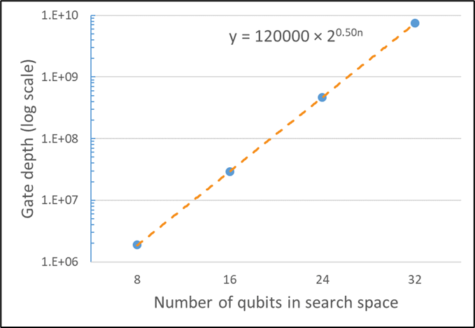
Figure 10: Gate Depth over Search Space Size for MD5 Preimage

Table 2 lists the results of a similar analysis, but this time varying the number of search targets instead of the size of the search space. (In this case, the search space was held constant at 16 qubits.) Fig. 11 plots the data with a power regression confirming that the gate depth falls off proportional to $\frac{1}{\sqrt{k}}$, with $k$ being the number of search targets. Again, this matches the expected time complexity.

Table 2: Cost of MD5 Preimage for Various Numbers of Search Targets

# of Search Targets	Depth	Width
1	29,252,464	801
2	20,708,556	801
3	16,943,444	801
4	14,626,452	801
5	13,033,520	801

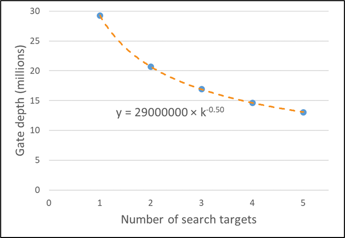
Figure 11: Gate Depth over Search Space Size for MD5 Preimage

While these are not actionable results in and of themselves, they serve as a “sanity check” that Grover’s algorithm was implemented correctly, and that the underlying methods used are sound.

3.2 Differences Between Hash Functions

The main result of this study is the data in Table 3, which lists the required gate depth and qubit width to conduct a preimage attack on each of the hash functions implemented. The number of qubits in the search space was kept constant at 16, with only one search target.

Table 3: Cost of Preimage For Various Hash Functions

Hash Function	Depth	Width
MD5	29,252,464	801
SHA-1	36,475,332	2913
SHA-224	38,953,918	2593
SHA-256	38,953,918	2593
SHA-384	99,089,086	6209
SHA-512	99,089,086	6209
SHA-512/224	99,089,086	6209
SHA-512/256	99,089,086	6209
SHA3-224	1,131,675	2161
SHA3-256	1,131,675	2193
SHA3-384	1,131,675	2193
SHA3-512	1,505,375	2449
SHAKE128-256	1,131,675	2193
SHAKE256-512	1,505,375	2449

Fig. 12 compares the gate depth of each function. Note the log scale. Clearly, the computational cost of a quantum attack against SHA-3 is much lower than that of MD5, SHA-1, and SHA-2. This is largely due to the fact that SHA-3 utilizes operations and permutations that translate more naturally to a quantum context, while the others rely primarily on arithmetic addition which is expensive on a quantum computer.

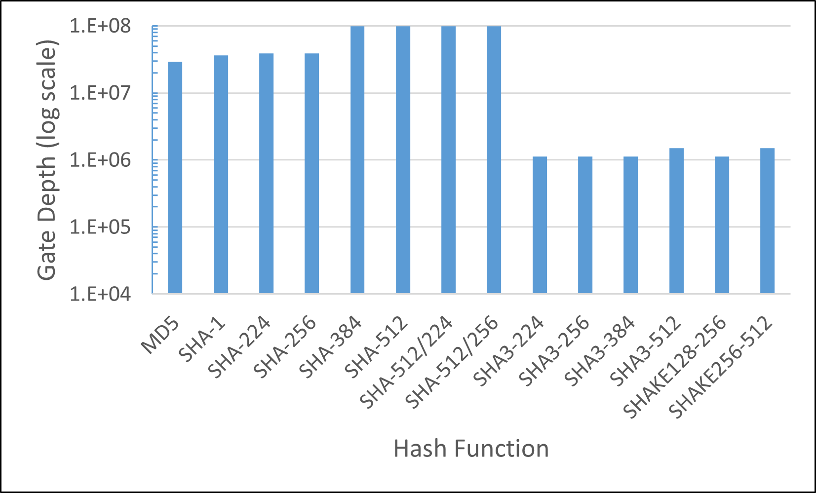
Figure 12: Gate Depth for Preimage of Various Hash Functions

The picture in Fig. 13 is a little different. When it comes to the number of qubits required, SHA-3 is comparable in cost to SHA-2 functions with a 256-bit state, but those with a 512-bit state are much more expensive. This suggests that, for example, SHA-512/256 is more quantum-resistant than SHA-256 and SHA3-256.

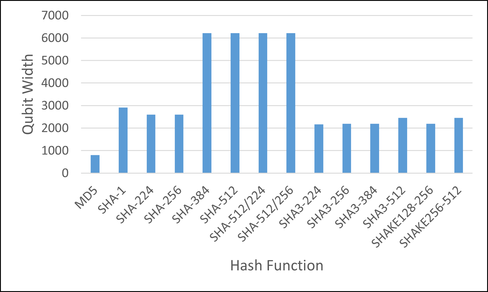
Figure 13: Qubit Width for Preimage of Various Hash Functions

4 Discussion

The results obtained show important differences in the computational costs associated with each hash function. Of particular interest is how SHA-3, a more recently developed algorithm, is cheaper to preimage on a quantum computer than the others (expect for MD5 in terms of qubit width). However, it should be noted that the quantum implementations of the hash functions used here are not guaranteed to be optimal. We directly translated the classical steps into quantum instructions, but new methods for creating more cost-efficient quantum oracles could be devised in the future.

The extent of the findings is also qualified by the limitations in the underlying quantum computing hardware, as well as some practical considerations when it comes to conducting preimage attacks against hash functions. These are discussed below.

4.1 Hardware Limitations

This paper takes a relatively abstract view of quantum computing, essentially at the level of quantum software. While Q# provides a simulator and resource estimator, support for running on a real live quantum computer is limited. And so, we do not consider computational costs associated with the underlying quantum hardware. The most important of these is quantum error correction.

On real quantum computers, the qubits are subjected to environmental noise that degrades or destroys their state over time. To perform useful computation, any errors that were introduced by noise must be fixed using quantum error correction (QEC). In a nutshell, QEC uses error codes to reduce the likelihood of error by introducing additional qubits. For example, a QEC scheme might use eight physical qubits to compose a single “logical” qubit, whose error rate is brought down to an acceptable level. Obviously, performing the error correction algorithm introduces additional costs in terms of both qubits and gates. These costs are so prohibitive to current-generation quantum computers that they are hard-pressed to maintain even a single logical qubit for practical applications. This means that any quantum program relying on error-free qubits (such as the ones discussed in this report), cannot be run at all in the near term, and will have large overhead costs associated with QEC into the future.

Another important hardware-related cost is introduced by the qubit topology. There are multiple approaches to how a qubit is physically realized in quantum hardware, and how they are arranged in space. For example, the qubits may be laid out in a 2D grid, and controlled gates such as CNOT can only be applied to adjacent qubits [16]. In that case, SWAP gates would be required to position the desired states in the appropriate location before each CNOT. To put it plainly, this becomes a total mess – you need optimization algorithms to minimize the number of SWAPs, and it may significantly increase the level of computational complexity. It remains to be seen what quantum hardware approach will be most successful, so for now it suffices to mention that this is likely to be a factor in any physical implementation of a quantum algorithm.

4.2 Practical Considerations of Preimage Attacks

When talking about a preimage attack against a cryptographic hash algorithm, typically no knowledge of the original input is assumed. That is, you are given a hash output and asked to find at least one corresponding input of any length. Assuming a theoretically perfect hash function, given any distinct input, there is an equal chance ($\frac{1}{2^{l}}$) of getting any of the possible $l$-bit outputs. Thus, the probability of getting a specific output after $n$ guesses follows a binomial distribution, $P(n)=1-(1-\frac{1}{2}^{l})^{n}$. Setting $n=2^{l}$ gives a probability of

$$P(2^{l})=1-(1-\frac{1}{2^{l}})^{2^{l}}\approx 1-\frac{1}{e}\textrm{ for large }l$$

That is, the probability that a preimage attack succeeds with $2^{l}$ guesses and no prior knowledge is about 63.2%. Of course, in a classical context, if you do not find a match you can just keep guessing and expect to find one eventually.

Now, consider Grover’s algorithm. It is not guess-and-check. Rather, it finds the matching input directly using amplitude amplification. However, the number of search targets must be specified. This is a problem because hash functions are not one-to-one; more than one distinct input can map to the same output. In other words, the number of search targets is not known in advance (although it follows a binomial probability distribution).

The software program we developed for this research supports simple strategies for trying Grover’s algorithm with different numbers of search targets. However, they were not used when estimating computational resources; one search target was assumed. This is because the search space was so small ($2^{16}$) that the probability of a collision existing is near zero. (There are more sophisticated methods of dealing with an unknown number of search targets; Boyer et al. lay out one such strategy in “Tight bounds on quantum searching” [18].)

In practice, and particularly for the current officially approved functions (SHA-2 and SHA-3), a search space of sufficient size to contain a collision with non-negligible probability is too big to search, even for Grover’s algorithm. Consider SHA-256. The search space would have to be somewhere near 256 bits before it is likely to contain a collision. But the gate depth of Grover’s algorithm applied to SHA-256 is $\mathrm{O}(2^{\frac{l}{2}})$, or $\mathrm{O}(2^{128})$. Even supposing one trillion operations per second, this would still take around $10^{19}$ years.

A more realistic situation is where the input length is known in advance, or it is at least limited in length. Suppose you intercept the SHA-256 hash of a password that you happen to know is 12 characters long (96 bits). Recovering the password is $\mathrm{O}(2^{96})$ using guess-and-check and $\mathrm{O}(2^{48})$ with Grover’s algorithm on a quantum computer. Assuming one billion operations per second, that is the difference between quadrillions of years and a few days. In scenarios like this, you are searching for exactly one target, and so the results shown in Section 3 are applicable.

5 Conclusion

This work provides an example of analyzing quantum algorithms through software. We used Microsoft’s QDK to study the practicality of quantum preimage attacks on classical hash functions. This involved implementing the hash functions as quantum oracles in Q#, validating their correctness using the Toffoli simulator, and then applying the built-in resource estimator to obtain computational complexity metrics. Through this process, we reduced the number of logical qubits required for the SHA-3 oracle by 40% compared to Amy et al.’s implementation. And our analysis concluded that the 512-bit state variants of SHA-2 are the most quantum-resistant out of the hash functions studied.

The advantage of this approach is that the algorithm must be explicitly expressed as a software program, so it leaves very little room for false assumptions about its actual behavior and complexity. Also, once the program is written and validated, the resource estimation can be performed automatically, rather than manually on paper. As quantum software frameworks like the QDK improve, the metrics reported can be more precise and tailored to the specific hardware platform the program is expected to run on. For example, IBM’s Qiskit platform allows the user to run quantum code on real quantum computers or perform simulations that introduce realistic errors [19].

5.1 Future Work

Here, we were limited to providing grounded estimates in terms of logical qubits with the QDK, since the width and depth of the programs written for this research were much too large to run on today’s NISQ-era devices. It must be emphasized that major blocking challenges exist in creating scalable, error-corrected quantum computers. Nevertheless, this type of analysis is critical in understanding the practical considerations when applying a quantum algorithm to a real-world problem, so that we can prepare appropriately for the threats and opportunities that advances in quantum computing technology will bring.

The logical next step would be to expand the library of classical functions implemented in quantum software so that Grover’s Algorithm can be applied. For example, Jaques et al. provide oracle implementations for AES-128, -192, and -256 in their paper, “Implementing Grover Oracles for Quantum Key Search on AES and LowMC” [20]. We could also improve the confidence and precision of our study by reproducing the implementations in other quantum software frameworks, such as Qiskit, and comparing the results of various resource estimation tools.

Going further, the approach we took can be replicated for other quantum algorithms. A standard library of common quantum applications implemented with multiple software frameworks could provide clear and precise benchmarks for quantum computers. The Standards and Performance Metrics Technical Advisory Committee of the Quantum Economic Development Consortium recently published a study in this vein where they developed and proposed application-oriented performance benchmarks and open-sourced their code [21]. By providing actual quantum programs to run, different quantum computers can be compared fairly, and the practicality of running an algorithm on various quantum systems can be studied in detail.

References

- Grover [1996] Lov K. Grover. A fast quantum mechanical algorithm for database search. In Proceedings of the Twenty-Eighth Annual ACM Symposium on Theory of Computing, STOC ’96, page 212–219, New York, NY, USA, 1996. Association for Computing Machinery. ISBN 0897917855. doi: 10.1145/237814.237866.
- Amy et al. [2016] Matthew Amy, Olivia Di Matteo, Vlad Gheorghiu, Michele Mosca, Alex Parent, and John Schanck. Estimating the cost of generic quantum pre-image attacks on sha-2 and sha-3, 2016. URL https://arxiv.org/abs/1603.09383.
- Clapis [2021] Joseph Clapis. A quantum dot plot generation algorithm for pairwise sequence alignment. Technical report, MITRE, 2021. URL https://arxiv.org/abs/2107.11346.
- Prousalis and Konofaos [2019] Konstantinos Prousalis and Nikos Konofaos. quantum pattern recognition method for improving pairwise sequence alignment. Scientific Reports, 9(1):7226, May 2019. URL https://www.nature.com/articles/s41598-019-43697-3.
- Svore et al. [2018] Krysta Svore, Martin Roetteler, Alan Geller, Matthias Troyer, John Azariah, Christopher Granade, Bettina Heim, Vadym Kliuchnikov, Mariia Mykhailova, and Andres Paz. Q#. Proceedings of the Real World Domain Specific Languages Workshop 2018 on - RWDSL2018, 2018. doi: 10.1145/3183895.3183901.
- Wootters and Zurek [1982] William K Wootters and Wojciech H Zurek. A single quantum cannot be cloned. Nature, 299(5886):802–803, 1982. URL https://www.nature.com/articles/299802a0.
- Merkle [1990] Ralph C. Merkle. A certified digital signature. In Gilles Brassard, editor, Advances in Cryptology — CRYPTO’ 89 Proceedings, pages 218–238, New York, NY, 1990. Springer New York. ISBN 978-0-387-34805-6. URL https://link.springer.com/chapter/10.1007/0-387-34805-0_21.
- Damgård [1990] Ivan Bjerre Damgård. A design principle for hash functions. In Gilles Brassard, editor, Advances in Cryptology — CRYPTO’ 89 Proceedings, pages 416–427, New York, NY, 1990. Springer New York. ISBN 978-0-387-34805-6. URL https://link.springer.com/chapter/10.1007/0-387-34805-0_39.
- Rivest [1992] Ronald L. Rivest. The md5 message-digest algorithm. RFC 1321, April 1992. URL https://doi.org/10.17487/RFC1321.
- Takahashi et al. [2009] Yasuhiro Takahashi, Seiichiro Tani, and Noboru Kunihiro. Quantum addition circuits and unbounded fan-out, 2009. URL https://arxiv.org/abs/0910.2530.
- 3rd and Jones [2001] Donald E. Eastlake 3rd and Paul Jones. Us secure hash algorithm 1 (sha1). RFC 3174, September 2001. URL https://doi.org/10.17487/RFC3174.
- of Standards and Technology [2015a] National Institute of Standards and Technology. Secure hash standard (shs). Technical Report FIPS 180-4, U.S. Department of Commerce, Washington, D.C., 2015a. URL https://doi.org/10.6028/NIST.FIPS.180-4.
- G. Bertoni and Assche [2007] M. Peeters G. Bertoni, J. Daemen and G. Van Assche. Sponge functions. In Ecrypt Hash Workshop, 2007. URL https://keccak.team/files/SpongeFunctions.pdf.
- of Standards and Technology [2015b] National Institute of Standards and Technology. Sha-3 standard: Permutation-based hash and extendable-output functions. Technical Report FIPS 202, U.S. Department of Commerce, Washington, D.C., 2015b. URL https://doi.org/10.6028/NIST.FIPS.202.
- National Academies of Sciences, Engineering, and Medicine [2019] National Academies of Sciences, Engineering, and Medicine. Quantum Computing: Progress and Prospects. The National Academies Press, Washington, DC, 2019. ISBN 978-0-309-47969-1. doi: 10.17226/25196.
- Kitaev [2003] A.Yu. Kitaev. Fault-tolerant quantum computation by anyons. Annals of Physics, 303(1):2–30, Jan 2003. ISSN 0003-4916. doi: 10.1016/s0003-4916(02)00018-0.
- Brassard et al. [1998] Gilles Brassard, Peter HØyer, and Alain Tapp. Quantum cryptanalysis of hash and claw-free functions. Lecture Notes in Computer Science, page 163–169, 1998. ISSN 1611-3349. doi: 10.1007/bfb0054319.
- Boyer et al. [1998] Michel Boyer, Gilles Brassard, Peter Høyer, and Alain Tapp. Tight bounds on quantum searching. Fortschritte der Physik, 46(4-5):493–505, Jun 1998. ISSN 1521-3978. doi: 10.1002/(sici)1521-3978(199806)46:4/5<493::aid-prop493>3.0.co;2-p.
- Anis et al. [2021] MD Sajid Anis et al. Qiskit: An open-source framework for quantum computing, 2021. URL https://doi.org/10.5281/zenodo.2573505.
- Jaques et al. [2020] Samuel Jaques, Michael Naehrig, Martin Roetteler, and Fernando Virdia. Implementing grover oracles for quantum key search on aes and lowmc. In 39th Annual International Conference on the Theory and Applications of Cryptographic Techniques, Zagreb, Croatia, May 10–14, 2020, Proceedings, volume 12105 of Lecture Notes in Computer Science. Springer, 2020. doi: 10.1007/978-3-030-45724-2_10. URL https://dx.doi.org/10.1007/978-3-030-45724-2_10.
- Lubinski et al. [2021] Thomas Lubinski, Sonika Johri, Paul Varosy, Jeremiah Coleman, Luning Zhao, Jason Necaise, Charles H. Baldwin, Karl Mayer, and Timothy Proctor. Application-oriented performance benchmarks for quantum computing, 2021. URL https://doi.org/10.48550/arXiv.2110.03137.