Photoinduced Prethermalization Phenomena in Correlated Metals

Abstract

We study prethermalization phenomena in weakly interacting Hubbard systems after electric-field pump pulses with finite duration. We treat the Hubbard interaction $U$ up to second order, applying the prethermalization paradigm for time-dependent interaction protocols, and the electric field strength beyond linear order. A scaling behavior with pulse duration is observed for the absorbed energy as well as individual prethermalized momentum occupation numbers, which we attribute to the leading quadratic orders in interaction and electric field. We show that a pronounced non-thermal momentum distribution can be created with pump pulses of suitable resonance frequencies, and discuss how to distinguish them from thermal states.

Marc Alexander, Marcus Kollar

Theoretical Physics III, Center for Electronic Correlations and Magnetism, Institute of Physics, University of Augsburg, 86135 Augsburg, Germany

1 Introduction

1.1 Photoexcitation of correlated electrons

Using pump-prope spectroscopy it is possible to observe the excitation and relaxation of interacting electron systems in real time, while potentially creating states or phases that do not occur in equilibrium [1, 2, 3]. Typically three stages are involved in this procedure [4]: an initial laser pulse which excites the electronic system, followed by its relaxation due to the scattering of electrons, and finally a transfer of energy to lattice degrees of freedom [5]. The photoexcited state may involve nonequilibrium steady states such as periodically driven Floquet states [6, 7, 8, 9, 10, 11], the dynamical generation of interactions [12, 13], or states at effectively negative temperature [14]. Its relaxation may pass through prethermal stages [15, 16, 17, 18] or be influenced by nonthermal fixed points [19] or dynamical critical points [20], while control of the final relaxation process is possible with coherent phonons [21, 22]. In this work we study the prethermal state for a single correlated band of photoexcited interacting electrons [23, 4]; a multiband case was recently discussed in Refs. [24, 25]. For a single band we study a Hubbard model with a general time dependence,

$$\hat{H}(t) =\sum_{ij\sigma}t_{ij}(t)\hat{c}^{\dagger}_{i\sigma}\hat{c}^{\phantom{\dagger}}_{j\sigma}+U\sum_{i}\hat{n}^{\phantom{\dagger}}_{i\uparrow}\hat{n}^{\phantom{\dagger}}_{i\downarrow}\,,$$ (1)

in terms of the usual fermionic creation, annihilation, and number operators for an electron at lattice site $\bm{R}_{i}$ with spin $\sigma$. Here the hopping amplitude $t_{ij}$ is the Fourier transform of the dispersion $\epsilon_{\bm{k}}$, and the Coulomb repulsion appears only in the Hubbard interaction $U$. For weak time-dependent interactions $U(t)$ such models exhibit prethermalization, i.e., on intermediate time scales a metastable state is attained in which quasiparticles are formed, the scattering of which then subsequently leads to thermalization [26, 27, 28, 29, 30]. As an application, the prethermalization regime can be used to limit the heating of periodically driven systems [8, 9, 11]. Here we study the characteristic features of field-induced prethermalized states for time-dependent but sufficiently weak interactions $U$ $>$ $0$. Our main result is that for a wave train containing $m$ pulses with frequency $\omega_{\text{pump}}$ $=$ $2\pi/T$ and electric field amplitude $E_{\text{ext}}$, the momentum occupation attains a prethermalization plateau after the pulse according to

$$\lim\limits_{m\to\infty}\frac{\langle\hat{n}_{{\bm{k}}\sigma}\rangle_{t>mT}-\langle\hat{n}_{{\bm{k}}\sigma}\rangle_{{{0}}}}{mT} =e^{2}a^{2}\,s\,\frac{\tilde{n}_{{\bm{k}}\sigma}^{(2)}(\omega_{\text{pump}})}{|\omega_{\text{pump}}+4\pi\text{i}\sigma(\omega_{\text{pump}})|^{2}}\,E_{\text{ext}}^{2}\,U^{2}\,,$$ (2)

for a Hubbard model with diagonal field direction on a hypercubic lattice with lattice constant $a$ as defined below in (8); we set $\hbar$ $=$ $1$. This scaling limit for long pump pulses involves a function $\tilde{n}_{{\bm{k}}\sigma}^{(2)}(\omega)$ which is given in Section 2.3 and depends functionally on the dispersion, while $s$ is a numerical prefactor of order unity depending on the specific envelope, e.g., $s$ $=$ $1/4$ for our pulse shape (7). Pumping with enveloped electric field pulses offers more flexibility than interaction protocols or continuous driving for the engineering of nontrivial metastable states. The denominator in (2) is due to an additional internal field generated in the sample by the external electric field [31] and helps to induce the prethermal state when the pump frequency is close to the resulting interaction-dependent resonance frequency.

The paper is organized as follows. In Section 1.2 we formulate a general weak-coupling approach for electric fields of arbitrary strength and use it in Section 1.3 to obtain the conductivity in lowest order. In Section 2.1 we discuss the time evolution during and after the field pulse in the prethermalization regime. The observed scaling with the pulse duration is explained in Section 2.2 for the absorbed energy and in Section 2.3 for individual momentum occupation numbers. In Section 2.4 we discuss the possibility of distinguishing the prethermal from the thermal state by optical spectroscopy and conclude in Section 3.

In a gauge with zero electric potential, the electric field enters only into the hopping amplitudes according to the Peierls substitution [32],

$$\bm{E}(\bm{r},t) =-\frac{1}{c}\frac{\partial\bm{A}(\bm{r},t)}{\partial t}\,,~{}~{}~{}~{}t_{ij}(t)=t_{ij}\,\text{e}^{-\tfrac{\text{i}e}{{\hbar}c}\int_{\bm{R}_{i}}^{\bm{R}_{j}}\!\text{d}\bm{r}\cdot\bm{A}(\bm{r},t)}~{}\to~{}t_{ij}\,\text{e}^{-\tfrac{\text{i}e}{{\hbar}c}({\bm{R}_{i}}-{\bm{R}_{j}})\cdot\bm{A}(t)}\,,$$ (3)

where in the last step the dipole approximation for the long-wavelength limit was used, so that within the sample the field $\bm{E}(t)$ $=$ $-\partial_{t}\bm{A}(t)/c$, $\bm{A}(t)$ $=$ $A(t)\hat{\bm{a}}$, is approximately homogeneous along a unit vector $\hat{\bm{a}}$, and the magnetic field vanishes. The electric field then enters only into the dispersion through $\delta\hat{H}_{0}(t)$,

$$\hat{H}_{0}+\delta\hat{H}_{0}(t) =\sum_{{\bm{k}}\sigma}\epsilon_{{\bm{k}}-\frac{e}{c}\bm{A}(t)}\,\hat{n}_{{\bm{k}}\sigma}\,.$$ (4)

Apart from the momentum occupation we will study in particular the current in the direction of $\hat{\bm{a}}$ and the change of the kinetic energy due to the field pulse, starting from the initial interacting ground state at time $t_{\text{ini}}$ $=$ $0$,

$$j(t) =\Big{\langle}{-{\frac{c}{{V}}}}\frac{\partial\hat{H}(t)}{\partial A(t)}\Big{\rangle}_{t}\,,~{}~{}~{}~{}\Delta E_{\text{kin}}(t)=\langle\hat{H}_{0}+\delta\hat{H}_{0}(t)\rangle_{t}-\langle\hat{H}_{0}\rangle_{{{0}}}\,,$$ (5)

where $V$ is the volume. However, the electric field in the Hamiltonian is not the same as the external field impinging on the sample. According to Ref. [31], in addition to the latter the field which is created in the sample due to Maxwell’s equations should also be taken into account. The total vector potential $\bm{A}(\bm{r},t)$ $=$ $\bm{A}_{\text{ext}}(\bm{r},t)$ $+$ $\bm{A}_{\text{sys}}(\bm{r},t)$ thus contains an internal part that obeys $(\partial_{t}^{2}-c^{2}\nabla^{2})\bm{A}_{\text{sys}}(\bm{r},t)=4\pi c\,\bm{j}_{\text{sys}}(\bm{r},t)$. For our case without spatial dependence this means $\partial_{t}^{2}\bm{A}_{\text{sys}}(t)/(4\pi c)$ $=$ $\bm{j}_{\text{sys}}(t)$ $=$ $j(t)\hat{\bm{a}}$, where the quantum-mechanical expectation value is identified with the classical current. In terms of the linear-response conductivity $\sigma(\omega)$ for the internal electric field, the conductivity for the external field is then obtained from the partial Fourier transform of the current $j(t)$ in the field direction as

$$j(\omega) =E_{\text{ext}}(\omega)\sigma_{\text{ext}}(\omega)=E(\omega)\sigma(\omega)\,,~{}~{}~{}~{}\sigma_{\text{ext}}(\omega)=\frac{\sigma(\omega)}{\epsilon(\omega)}\,,~{}~{}~{}~{}\epsilon(\omega)=1+\text{i}\frac{4\pi}{\omega}\sigma(\omega)\,,$$ (6)

via $j(\omega)$ $=$ $\text{i}\omega E_{\text{sys}}(\omega)/(4\pi)$ and $E_{\text{ext}}(\omega)$ $=$ $E(\omega)-E_{\text{sys}}(\omega)$. The total internal field $E(\omega)$ in the Hamiltonian (3) thus equals $E(\omega)$ $=$ $E_{\text{ext}}(\omega)/\epsilon(\omega)$ in linear order in the field.

For our present study, we will start from a given internal field pulse and obtain the response of the interacting system to all orders in the field, but perturbatively in the interaction. For the relation between internal and external field, however, only the linear-response connection (6) will be used, for which the required conductivity is obtained perturbatively in the interaction in subsection 1.3. A more realistic nonlinear description of the relation between internal and external field is beyond the scope of the present work.

We assume a pulse for which the Hamiltonian is the same before and after the pulse, which is appropriate for a metallic system even if the external field were to have different vector potentials before and after the pulse. Specifically, we consider a (real-valued) enveloped field pulse for the internal electric field with frequency $\omega_{\text{pump}}$ $=$ $2\pi/T$ acting from time $t_{\text{ini}}$ $=$ $0$ to $t_{\text{fin}}$ $=$ $mT$, i.e., a wave train over an integer number $m$ of periods, shown in Figure 1,

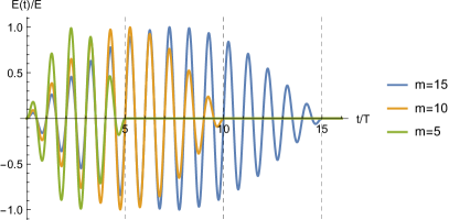
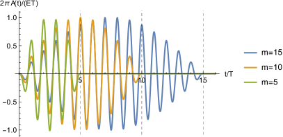
Figure 1: Normalized dimensionless electric field (left) and vector potential (right).

$$E(t) =-\frac{1}{c}\frac{\partial A(t)}{\partial t}=E\sin\left(\frac{2\pi t}{T}\right)\sin\left(\frac{\pi t}{mT}\right)=\sum_{j=1}^{4}E_{j}\,\text{e}^{\text{i}t\omega_{j}}\,,~{}~{}~{}~{}E_{\text{ext}}(t)=\sum_{j=1}^{4}E_{\text{ext},j}\,\text{e}^{\text{i}t\omega_{j}}\,,$$ (7)

where $E_{1+2j}$ $=$ $E_{2+2j}$ $=$ $(-1)^{1+j}E/4$ and $\omega_{1+2j}$ $=$ $-\omega_{2+2j}$ $=$ $[1+(-1)^{j}/(2m)]\,\omega_{\text{pump}}$ for $j$ $=$ $0,1$. The Fourier components $E_{j}$ of the internal field at frequency $\omega_{j}$ translate into corresponding components $E_{\text{ext},j}$ $=$ $\epsilon(\omega_{j})E_{j}$ for the external field according to (6).

To illustrate our general results such as (2), we will perform explicit evaluations following Ref. [23], i.e., using next-neighbor hopping $t_{ij}$ $=$ $t^{*}/2\sqrt{d}$ for a hypercubic lattice in the limit of infinite dimensions $d$ and assuming a diagonal field direction, $\hat{\bm{a}}$ $=$ $(1,1,\ldots,1)$. This limit of high dimensions [33] corresponds to dynamical mean-field theory, which describes three-dimensional correlated electron materials in equilibrium [34, 35] and nonequilibrium [4] well in general. The diagonal field direction is representative for the high-dimensional limit, as it does not require further scalings with powers of $d$ that would be needed, e.g., for a bond direction. The diagonal field direction also leads to technical simplifications, as the kinetic energy, the cosine and sine dispersions, density of states and joint density of states take the following form in the limit of large $d$,

$$\hat{H}_{0}+\delta\hat{H}_{0}(t) =\hat{H}_{0}\cos A(t)+\hat{\bar{H}}_{0}\sin A(t)\,,~{}~{}~{}~{}\hat{H}_{0}=\sum_{{\bm{k}}\sigma}\epsilon_{\bm{k}}\,\hat{n}_{{\bm{k}}\sigma}\,,~{}~{}~{}~{}\hat{\bar{H}}_{0}=\sum_{{\bm{k}}\sigma}\bar{\epsilon}_{\bm{k}}\,\hat{n}_{{\bm{k}}\sigma}\,,$$ (8a)

$$\epsilon_{\bm{k}} =-\frac{t^{*}}{\sqrt{d}}\sum\limits_{j=1}^{d}\cos(k_{j}a)\,,~{}~{}~{}~{}\bar{\epsilon}_{\bm{k}}=-\frac{t^{*}}{\sqrt{d}}\sum\limits_{j=1}^{d}\sin(k_{j}a)\,,$$ (8b)

$$\rho(\epsilon) =\frac{1}{L}\sum_{\bm{k}}\delta(\epsilon-\epsilon_{\bm{k}})=\frac{\text{e}^{-\epsilon^{2}/{t^{*}}^{2}}}{\sqrt{\pi}t^{*}}\,,~{}~{}~{}~{}\rho(\epsilon,\bar{\epsilon})=\frac{1}{L}\sum_{\bm{k}}\delta(\epsilon-\epsilon_{\bm{k}})\delta(\bar{\epsilon}-\bar{\epsilon}_{\bm{k}})=\frac{\text{e}^{-(\epsilon^{2}+\bar{\epsilon}^{2})/{t^{*}}^{2}}}{\pi{t^{*}}^{2}}\,,$$ (8c)

for $L$ lattice sites. Here we set $\hbar$, $c$, $a$ to unity. We also set $t^{*}$ $=$ $1$ and consider only a half-filled band, with uncorrelated kinetic energy $E_{\text{kin}}^{(0)}(0)$ $=$ $-\frac{1}{2\sqrt{\pi}}$ $\simeq$ $-0.282$. Our units are thus $\hbar/t^{*}$ for time, $t^{*}/\hbar$ for frequency, $\hbar c/(ea)$ for $A(t)$, $t^{*}/(ea)$ for $E(t)$, $t^{*}/(a^{2}\hbar)$ for $j(t)$, $e^{2}t^{*}/(\hbar^{2}a)$ for $\sigma(t)$, and $e^{2}/(\hbar a)$ for $\sigma(\omega)$. The term $\sigma(\omega)/\omega$ in (6) requires us to fix the scale $\hbar c/(at^{*})$; we estimate $a\cdot|E_{\text{kin}}^{(0)}(0)|$ $\simeq$ $4$ Å $\cdot$ eV to be a representative value and use this in explicit calculations involving $\sigma_{\text{ext}}(\omega)$. Evaluations for this setup can be performed efficiently using integration techniques described in the Appendix. In the following we will refer to the interacting model (1) and (8) simply as the Hubbard model with diagonal field direction. We will denote $\hat{n}_{{\bm{k}}\sigma}$ as $\hat{n}_{\epsilon\bar{\epsilon}\sigma}$ when it depends only on $\epsilon_{\bm{k}}$ and $\bar{\epsilon}_{\bm{k}}$.

1.2 Weak-coupling theory

For the initial and time-evolved states of an interacting Hamiltonian we use a perturbative formulation which is also useful for prethermalization phenomena after general interaction protocols $U(t)$ as discussed separately elsewhere [36]. For a general time-dependent Hamiltonian $\hat{H}(t)$ $=$ $\hat{H}_{0}(t)$ $+$ $g\hat{V}(t)$, an operator $\hat{A}$ evolved in the interaction picture reads

$$\hat{S}^{\dagger}(t)\hat{A}_{I}({t})\hat{S}(t)=\sum\limits_{n=0}^{\infty}(ig)^{n}\!\int_{0}^{t}\!\text{d}t_{1}\ldots\!\int_{0}^{t_{n-1}}\!\text{d}t_{n}\big{[}\hat{V}_{I}(t_{n}),\ldots\big{[}\hat{V}_{I}(t_{1}),\hat{A}_{I}({t})\big{]}\ldots\big{]}\,,$$ (9)

with the interaction picture propagator $\hat{S}(t)$ $=$ $\hat{U}^{\dagger}_{0}(t)\hat{U}(t)$, defined in terms of the propagators $\hat{U}_{0}(t)$ and $\hat{U}(t)$ of $\hat{H}_{0}(t)$ and $\hat{H}_{0}(t)$ $+$ $g\hat{V}(t)$, respectively, and $\hat{O}_{I}(t)$ $=$ $\hat{U}^{\dagger}_{0}(t)\hat{O}(t)\hat{U}_{0}(t)$ for any Schrödinger operator $\hat{O}(t)$.

For our Hamiltonian (4), the initial interacting ground state of $\hat{H}(0)$ $=$ $\hat{H}_{0}$ $+$ $g\hat{V}$ (where $g$ $=$ $U$ and $\hat{V}$ $=$ $\sum_{i}\hat{n}^{\phantom{\dagger}}_{i\uparrow}\hat{n}^{\phantom{\dagger}}_{i\downarrow}$) at $t$ $=$ $0$ is time-evolved with the additional kinetic energy term $\delta\hat{H}_{0}(t)$, which vanishes before and after the electric field pulse. We consider an auxiliary Hamiltonian in which the interaction term is switched on adiabatically for negative times, so as to generate the interacting initial state from the corresponding noninteracting eigenstate $|\Psi(t=-\infty)\rangle$ $=$ $|\Psi_{0}\rangle$ with $\hat{H}_{0}|\Psi_{0}\rangle$ $=$ $E_{0}|\Psi_{0}\rangle$ and expectation values $\langle\cdots\rangle_{(0)}$; by contrast expectation values in the initial interacting eigenstate are denoted by $\langle\cdots\rangle_{t=0}$ $=$ $\langle\cdots\rangle_{{{0}}}$. Namely we set

$$\hat{H}(t)=\hat{H}_{0}+\delta\hat{H}_{0}(t)+g\,f(t)\,\hat{V}\,,~{}~{}~{}~{}f(t)=\begin{cases}\text{e}^{\delta t}&\text{if~{}}t<0,\\ 1&\text{if~{}}t\geq 0,\end{cases}~{}~{}~{}~{}\delta\to 0^{+}\,.$$ (10)

Here $\hat{H}_{0}+\delta\hat{H}_{0}(t)$ has the same set of eigenstates $\{|\Psi_{l}\rangle\}$ as $\hat{H}_{0}$. The noninteracting propagator for $t$ $\geq$ $0$ is therefore simply $\hat{U}_{0}(t)$ $=$ $\exp(-\text{i}\int_{0}^{t}\text{d}\tau\,[\hat{H}_{0}+\delta\hat{H}_{0}(\tau)])$. Expanding in the interaction strength $g$ we have for any observable $\hat{A}$,

$$\langle\hat{A}\rangle_{t} =\langle\hat{A}\rangle_{(0)}+g\Delta A^{(1)}(t)+O(g^{2})\,,$$ (11a)

$$\Delta A^{(1)}(t) =\text{i}\int_{-\infty}^{t}\!\text{d}t_{1}\,f(t_{1})\langle\big{[}\hat{V}_{I}(t_{1}),\hat{A}_{I}({t})\big{]}\rangle_{(0)}=\sum_{l}V_{0l}\,A_{l0}\,\varphi_{l}^{(1)}(t)+\text{c.c.}\,,$$ (11b)

$$\varphi_{l}^{(1)}(t) =\text{i}\int_{-\infty}^{t}\!\text{d}t_{1}\,f(t_{1})\text{e}^{\text{i}\int_{t_{1}}^{t}\!\text{d}\tau\,\Delta E_{l}+\delta e_{l}(\tau)}=-\frac{1}{\Delta E_{l}}+\text{i}\int_{0}^{t}\!\text{d}t_{1}\,\text{e}^{\,i(t-t_{1})\Delta E_{l}}\big{(}\text{e}^{\text{i}\int_{t_{1}}^{t}\!\text{d}\tau\,\delta e_{l}(\tau)}-1\big{)}\,,$$ (11c)

where we used the abbreviations $\langle\Psi_{l}|\hat{A}|\Psi_{m}\rangle$ $=$ $A_{lm}$, $\Delta E_{l}$ $=$ $E_{l}-E_{0}$, $\delta\hat{H}_{0}(t)|\Psi_{l}\rangle$ $=$ $\delta E_{l}(t)|\Psi_{l}\rangle$, $\delta e_{l}(t)$ $=$ $\delta E_{l}(t)-\delta E_{0}(t)$. We label observables that commute with $\hat{H}_{0}$ as second-order observables $\hat{a}$ (because the first-order term vanishes for them), otherwise as first-order observables $\hat{A}$. For a second-order observable we have

$$\langle\hat{a}\rangle_{t} =\langle\hat{a}\rangle_{(0)}+g^{2}\Delta a^{(2)}(t)+O(g^{3})\,,$$ (12a)

$$\Delta a^{(2)}(t) =-\int_{-\infty}^{t}\!\text{d}t_{1}\int_{-\infty}^{t_{1}}\!\text{d}t_{2}\,f(t_{1})f(t_{2})\langle\big{[}\hat{V}_{I}(t_{2}),\big{[}\hat{V}_{I}(t_{1}),\hat{a}\big{]}\big{]}\rangle_{0}=\sum_{l}|V_{0l}|^{2}\Delta a_{l}\varphi_{l}^{(2)}(t)\,,$$ (12b)

$$\varphi_{l}^{(2)}(t) =\int_{-\infty}^{t}\!\text{d}t_{1}\int_{-\infty}^{t_{1}}\!\text{d}t_{2}\,f(t_{1})f(t_{2})\text{e}^{\text{i}\int_{t_{2}}^{t_{1}}\!\text{d}\tau\,\Delta E_{l}+\delta e_{l}(\tau)}+\text{c.c.}$$

$$=\frac{1}{\Delta E_{l}^{2}}-2\,\text{Re}\int_{0}^{t}\!\text{d}t_{1}\int_{0}^{t_{1}}\!\text{d}t_{2}\,\exp\Big{(}\text{i}\int_{t_{2}}^{t_{1}}\!\text{d}t^{\prime}\,(\Delta E_{l}+\delta e_{l}(t^{\prime}))\Big{)}\frac{\delta e_{l}(t_{2})}{\Delta E_{l}}\,,$$ (12c)

where $\hat{a}|\Psi_{l}\rangle=a_{l}|\Psi_{l}\rangle$, and $\Delta a_{l}=a_{l}-a_{0}$. Without electric field, $\delta e_{l}(t)=0$, both (11) and (12) reduce to the standard perturbative result for the interacting ground state.

1.3 Relation between internal and external field in linear response

As discussed in the first subsection, below we will use a given internal field pulse (7), which is related to the external field pulse according to (6) in linear order in the field. We therefore use the expressions of the previous subsection to obtain the conductivity in second order in the interaction. Expanding to $O(A^{2})$ with $\bm{A}(t)$ $=$ $A(t)\hat{\bm{a}}$ gives (with $\hbar$, $c$, $a$ set to unity)

$$\!\!\!\!\!\!\!\!\hat{j}(t)=-\frac{1}{{L}}\frac{\partial\hat{H}(t)}{\partial A(t)}=e\hat{H}_{0}^{(1)}-{e^{2}}A(t)\hat{H}_{0}^{(2)}+O(A^{2})\,,\;\hat{H}_{0}^{(n)}={\frac{1}{L}}\sum_{k\sigma}\epsilon^{(n)}_{{\bm{k}}}\hat{n}_{{\bm{k}}\sigma}\,,\;\epsilon^{(n)}_{{\bm{k}}}=\frac{\partial^{n}\epsilon_{{\bm{k}}+\hat{\bm{a}}{x}}}{\partial x^{n}}\Big{|}_{x=0}\,.\!\!\!$$ (13)

For a field that is zero before $t_{\text{ini}}$ $=$ $0$, the linear-response result for the current, $j(t)$ $=$ $\langle\hat{j}\rangle_{t}$, then comprises the usual diamagnetic and paramagnetic contribution to the conductivity,

$$j(t) =\int_{0}^{t}\!\text{d}\tau\,E(\tau)\sigma(t,\tau)+O(E^{2})\,,~{}~{}\sigma(t,\tau)=\sigma^{\text{dia}}(t)+\sigma^{\text{pm}}(t,\tau)\,,$$ (14a)

$$\sigma^{\text{dia}}(t) ={e^{2}}\,\langle\hat{H}_{0}^{(2)}\rangle_{t}\,,~{}~{}\sigma^{\text{pm}}(t,\tau)=\text{i}{e^{2}}\int_{0}^{t}\!\text{d}\tau^{\prime}\,\langle[\hat{H}_{0}^{(1)}(\tau^{\prime}),\hat{H}_{0}^{(1)}(t)]\rangle_{{{0}}}\,.$$ (14b)

where the time dependences of $\hat{H}_{0}^{(1)}$ are in the Heisenberg picture of the Hamiltonian without field. If that Hamiltonian is time-independent this simplifies to $\sigma^{\text{dia}}(t)$ $\to$ $\sigma^{\text{dia}}$, $\sigma^{\text{pm}}(t,\tau)$ $\to$ $\sigma^{\text{pm}}(t-\tau)$, and $j(\omega)$ $=$ $E(\omega)\sigma(\omega)$. For the interacting Hamiltonian $\hat{H}(0)$ $=$ $\hat{H}_{0}$ $+$ $g\hat{V}$ we use (12) to find in the leading orders in $g$ that

$$\sigma^{\text{dia}} =\sigma^{\text{dia},(0)}+g^{2}\sigma^{\text{dia},(2)}+O(g^{3})\,,~{}~{}\sigma^{\text{dia},(0)}={e^{2}}\,\langle\hat{H}_{0}^{(2)}\rangle_{0}\,,~{}~{}\sigma^{\text{dia},(2)}={e^{2}}\sum_{l}|V_{0l}|^{2}\frac{\Delta E_{l}^{(2)}}{\Delta E_{l}^{2}}\,,\!\!$$ (15a)

$$\!\!\!\!\!\!\sigma^{\text{pm}}(t-\tau) =g^{2}\sigma^{\text{pm},(2)}(t-\tau)+O(g^{3})\,,~{}\sigma^{\text{pm},(2)}(t)={e^{2}}\sum_{l}|V_{0l}|^{2}2(\Delta E^{(1)}_{l})^{2}\,\frac{\cos(\Delta E_{l}t)-1}{\Delta E_{l}^{3}}\,.$$ (15b)

with $\hat{H}_{0}^{(n)}|\Psi_{l}\rangle=E_{l}^{(n)}|\Psi_{l}\rangle$ and $E_{l}^{(n)}-E_{0}^{(n)}=\Delta E_{l}^{(n)}$, and the constant $\sigma^{\text{dia}}$ leading to the familiar Drude peak in the partial Fourier transform, $\sigma^{\text{dia}}(\omega)$ $=$ $\text{i}\sigma^{\text{dia}}/(\omega+\text{i}\delta)$, $\delta$ $\to$ $0^{+}$.

We evaluate these expressions for the Hubbard model with diagonal field direction (8), using weight functions $a_{n}(b)$ to represent Gaussian integrals as described in (43) of the Appendix. For coupling $g$ $=$ $U$ and with ${e^{2}}$ $=$ $1$, $t^{*}$ $=$ $1$, we have $\hat{H}_{0}^{(2)}=-\hat{H}_{0}$ and $\hat{H}_{0}^{(1)}=\hat{\bar{H}}_{0}$, leading to

$$\sigma(\omega) =\text{i}\frac{\sigma^{\text{dia},(0)}+U^{2}\sigma^{\text{dia},(2)}}{\omega+\text{i}\delta}+U^{2}\sigma^{\text{pm}(2)}(\omega)+O(U^{3})\,,$$ (16a)

$$\sigma^{\text{dia},(0)} =\frac{1}{2\sqrt{\pi}}\simeq 0.282\,,~{}~{}~{}~{}\sigma^{\text{dia},(2)}=-\int_{\frac{1}{4}}^{1}\!\text{d}b\,\frac{a_{4}(b)}{2\sqrt{\pi^{3}b^{3}}}\simeq-0.0659\,,$$ (16b)

$$\sigma^{\text{pm},(2)}(\omega) =\int_{\frac{1}{4}}^{1}\!\text{d}b\,\frac{2a_{4}(b)}{\sqrt{b\pi^{3}}}\bigg{(}\frac{-\text{i}}{\omega+\text{i}\delta}+\sqrt{\pi b}\,\text{e}^{-\omega^{2}b}+2\text{i}\sqrt{b}\,\text{D}_{+}(\sqrt{b}\omega)\bigg{)}\,,$$ (16c)

in terms of the Dawson function $\text{D}_{+}(x)$ $=$ $\text{e}^{-x^{2}}\int_{0}^{x}\!\text{d}t\,\text{e}^{t^{2}}$ and the weight function $a_{4}(b)$ of (47). The corresponding optical conductivity $\sigma_{\text{ext}}(\omega)$ for the external field is then calculated by inserting this result into (6) and is shown in Figure 2 with parameters as given below (8).

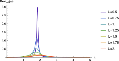
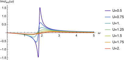
Figure 2: Optical conductivity $\sigma_{\text{ext}}$ with respect to the external field according to (6) for the Hubbard model with diagonal field direction (8), as given in (16). Here $\sigma_{\text{ext}}$ is in units of $e^{2}/(\hbar a)$ and $\omega$ in units of $t^{*}/\hbar$, and we have chosen $a\cdot|E_{\text{kin}}^{(0)}(0)|$ $=$ $4$ Å $\cdot$ eV, see remarks below (8).

In its denominator we keep $\epsilon(\omega)$ as a series in $U$ and do not expand it into the numerator. Similar to the result for the absorbed power [31], this denominator suppresses the zero-frequency pole for finite $U$ and turns it into a resonance at $\omega_{*}$, which approaches $\omega_{*}$ $=$ $\sqrt{2\sqrt{\pi}}$ $\simeq$ $1.88$ (in units of $t^{*}$ $=$ $1$) in the noninteracting limit.

2 Nonperturbative effects of a pump pulse with finite duration

2.1 Pulse-induced transient states and prethermalization

We consider the enveloped pump pulse $E(t)$ of (7), which is shown in Figure 1 together with its vector potential $A(t)$. For simplicity we will focus on the effect of this given internal field $E(t)$ on an interacting system, as the relation to the external field $E_{\text{ext}}(t)$ also involves the interaction according to (6)-(7). Because the momentum occupation numbers $\langle\hat{n}_{{\bm{k}}\sigma}\rangle_{t}$ are second-order observables we expand the observables $j(t)$ and $E_{\text{kin}}(t)$ of (5) by means of (12), $E_{\text{kin}}(t)$ $=$ $E_{\text{kin}}^{(0)}+g^{2}E_{\text{kin}}^{(2)}(t)+O(g^{3})$, $j(t)$ $=$ $j^{(0)}(t)+g^{2}j^{(2)}(t)+O(g^{3})$. For the Hubbard model with diagonal field direction (8) the time-dependent zeroth-order terms of kinetic energy and current are depicted in Figure 3. After the pulse they have returned to their initial values as the momentum occupation numbers remain constant in the noninteracting case. In the presence of interactions, the electric field induces changes that are depicted in Figure 4, in which the change in the double occupation, $\Delta D(t)$ $=$ $\langle\hat{n}^{\phantom{\dagger}}_{i\uparrow}\hat{n}^{\phantom{\dagger}}_{i\downarrow}\rangle_{t}$ $-$ $\langle\hat{n}^{\phantom{\dagger}}_{i\uparrow}\hat{n}^{\phantom{\dagger}}_{i\downarrow}\rangle_{0}$, a first-order observable, is also plotted. The averaged quantities follow the electric field amplitude closely. Individual momentum occupation numbers are not gauge independent during the pulse [4]; for our gauge they show slowly varying behavior with slight modulations during one period $T$. We further note that even for the very strong fields $E\geq 1$ considered here, the approximate field dependence is linear in $E$ for $j^{(2)}(t)$ and quadratic for $D^{(1)}(t)$ and $E_{\text{kin}}^{(2)}(t)$, which will be further studied in the next subsection. At the end of the field pulse these quantities undergo a further relaxation. As a first-order observable the double occupation relaxes to its value prior to the pulse, while the current relaxes to zero as it is a first-order observable in the electric field. The kinetic energy and the momentum occupation numbers are second-order observables in interaction strength and in the electric field and as such relax to a finite value on a time-scale on the order of $1/t_{*}$ $\equiv$ $1$. At second order in the interaction this is the prethermalization regime during which quasiparticles are formed, analogous to the case of time-dependent interaction protocols [15, 26, 16], and the kinetic energy and double occupation are already thermalized on this time scale. Further relaxation of individual momentum occupation numbers is expected due to the scattering of quasiparticles, but which we do not consider here.

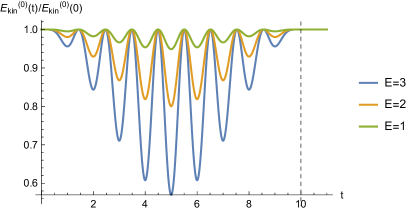
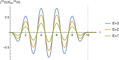
Figure 3: Normalized kinetic energy (left) and current (right) for the noninteracting ($U$ $=$ $0$) Hubbard model with diagonal field direction (8) subjected to the pump pulse (7) with $T$ $=$ $2$, $m$ $=$ $5$. Here the units are $\hbar/t^{*}$ for time, $t^{*}/(a^{2}\hbar)$ for current, $t_{*}$ for energy, and $t^{*}/(ea)$ for electric field, see remarks below (8).

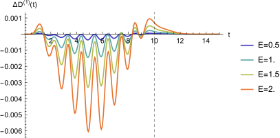
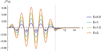
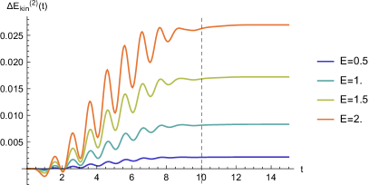
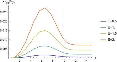
Figure 4: Leading contributions (in order $U^{n}$ as indicated by the upper index ⁽ⁿ⁾) to the change in double occupation (top left), current (top right), kinetic energy (bottom left) and momentum occupation number with $\epsilon_{\bm{k}}$ $=$ $\bar{\epsilon}_{\bm{k}}$ $=$ $0$ (bottom right) for the Hubbard model with diagonal field direction (8) subjected to the pump pulse (7) with $T$ $=$ $2$, $m$ $=$ $5$. Here the units are $\hbar/t^{*}$ for time, $t^{*}/(a^{2}\hbar)$ for current, $t_{*}$ for energy, and $t^{*}/(ea)$ for electric field, see remarks below (8).

2.2 Scaling behavior of the absorbed energy

From Figures 3 and 4 it is apparent that the electronic response scales approximately with the field amplitude, as we now analyze in further detail. Since the double occupation eventually returns to its initial value, the change in kinetic energy corresponds to the absorbed electric field energy. Its leading term in the electric field, $\Delta E_{\text{kin}}^{(2)}(t)$ $=$ $E^{2}\Delta E_{\text{kin}}^{(2,2)}(t)+O(E^{3})$ has a long-time limit that exhibits an approximate linear scaling with the pulse duration $t_{\text{fin}}$ $=$ $mT$ as shown in Figure 5.

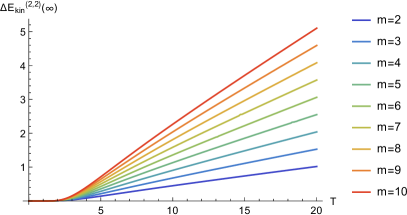
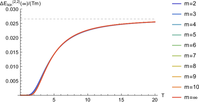
Figure 5: Prethermalization plateau of the kinetic energy (in order $U^{2}E^{2}$) for the Hubbard model with diagonal field direction (8) subjected to the pump pulse (7), unscaled (left) and scaled by pulse duration (right) for varying number of pulse oscillations $m$ and periods $T$. The limit of long pulse durations ($m$ $=$ $\infty$) corresponds to (21). Here the units are $\hbar/t^{*}$ for time, $t_{*}$ for energy, and $t^{*}/(ea)$ for electric field, see remarks below (8).

All the plotted prethermalization plateaus $\Delta E_{\text{kin}}^{(2,2)}(\infty)/mT$ collapse quite well onto a single curve, which should thus be described by the absorbed energy in the limit $m\to\infty$ of long pulse durations, which we now calculate. In leading order in the field we obtain for the absorbed field energy,

$$\delta\hat{H}_{0}(t) =-\frac{{e}}{c}A(t)\hat{H}_{0}^{(1)}+O(A^{2})\,,$$ (17a)

$$\Delta\langle\hat{H}\rangle_{t} =\frac{-1}{c^{2}}\int_{0}^{t}\!\text{d}t_{1}\int_{0}^{t_{1}}\!\text{d}t_{2}\,A(t_{1})A(t_{2})\,\langle{e^{2}}\,\big{[}\hat{H}_{0}^{(1)}(t_{2}),\big{[}\hat{H}_{0}^{(1)}(t_{1}),\hat{H}\big{]}\big{]}\rangle_{{{0}}}+O(A^{3})\,,$$ (17b)

for a general interaction, in which we recognize the expectation value as $\partial^{2}\sigma^{\text{pm}}(t)/\partial t^{2}|_{t=t_{1}-t_{2}}$, involving the paramagnetic conductivity of (14); as in that equation, the time dependences of $\hat{H}_{0}^{(1)}$ in (17) are in the Heisenberg picture of the Hamiltonian without field. To establish the approximate scaling with the pulse duration, we use a Fourier representation and consider only times $t$ after the end of the pulse,

$$\Delta\langle\hat{H}\rangle_{t>t_{\text{fin}}} =\int\!\text{d}\omega\,\frac{\omega^{2}\,\text{Re}\{\sigma^{\text{pm}}(\omega)\}}{c^{2}\pi}\int_{0}^{t_{\text{fin}}}\!\text{d}t_{1}\int_{0}^{t_{1}}\!\text{d}t_{2}\,A(t_{1})A(t_{2})\text{e}^{\text{i}(t_{1}-t_{2})(\omega+\text{i}\delta)}+O(A^{3})\,,$$ (18)

in which real part of the partial Fourier transform $\sigma^{\text{pm}}(\omega)$ appears since $\sigma^{\text{pm}}(t)$ is real and symmetric. For any (real-valued) electric field pulse that can be decomposed as $E(t)$ $=$ $\sum_{j}E_{j}\text{e}^{\text{i}t\omega_{j}}$ as in (7), we obtain in leading order in the pulse duration $t_{\text{fin}}$ that

$$\frac{1}{c^{2}}\int_{0}^{t_{\text{fin}}}\!\text{d}t_{1}\int_{0}^{t_{1}}\!\text{d}t_{2}\,A(t_{1})A(t_{2})\text{e}^{\text{i}(t_{1}-t_{2})(\omega+\text{i}\delta)}=\sum_{j}\frac{|E_{j}|^{2}}{\omega_{j}^{2}}\frac{\text{i}t_{\text{fin}}}{\omega+\text{i}\delta-\omega_{j}}+O(t_{\text{fin}}^{0})$$ (19)

Performing the limit $\delta$ $\to$ $0^{+}$ and collecting the delta contributions $(\omega+\text{i}\delta-\omega_{j})^{-1}\to-\text{i}\pi\delta(\omega-\omega_{j})$ gives us the following general result for the scaled long-time limit of the absorbed energy,

$$\lim\limits_{t_{\text{fin}}\to\infty}\frac{\Delta\langle\hat{H}\rangle_{t>t_{\text{fin}}}}{t_{\text{fin}}} =\sum_{j}|E_{j}|^{2}\,\text{Re}\{\sigma^{\text{pm}}(\omega_{j})\}+O(E^{3})\,.$$ (20)

This result for the absorbed power is still independent of the interaction. For the wave train (7) with $m$ pulses of period $T$ $=$ $2\pi/\omega_{\text{pump}}$ and in leading order in the interaction it becomes

$$\lim\limits_{m\to\infty}\frac{\Delta\langle\hat{H}\rangle_{t>mT}}{mT}=\frac{1}{4}\,E^{2}\,U^{2}\,\text{Re}\{\sigma^{\text{pm},(2)}(\omega_{\text{pump}})\}+O(E^{3}U^{2})+O(E^{2}U^{3})\,,$$ (21)

where the numerical prefactor is particular to our specific pulse shape. In Figure 5 this expression is plotted with the label $m$ $=$ $\infty$ and calculated from the paramagnetic conductivity in (16c) for the Hubbard model with diagonal field direction (8). We conclude that for sufficiently long pulses, the absorbed power is well approximated by the leading orders in field and interaction for all periods $T$. Relations similar to (20)-(21) between the absorbed power and the conductivity for essentially continuous pulses were also discussed in [31]. In the limit of long pulse durations we can replace the internal field amplitude $E$ in (21) by $E_{\text{ext}}(\omega_{\text{pump}})/\epsilon(\omega_{\text{pump}})$ to obtain the dependence on the external field, as further discussed in the next subsection.

2.3 Scaling behavior of the momentum distribution

As the kinetic energy already thermalizes at the prethermal stage, its plateau corresponds to the energy absorbed from the pump pulse. Nevertheless the prethermal state differs from the eventual thermal state in its momentum occupation numbers of individual modes, as we now discuss. For them we also observe scaling behavior, as shown for one momentum in Figure 6,

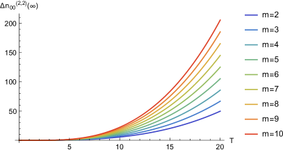
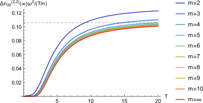
Figure 6: Prethermalization plateau of the momentum occupation (in order $U^{2}E^{2}$) with $\epsilon_{\bm{k}}$ $=$ $\bar{\epsilon}_{\bm{k}}$ $=$ $0$ for the Hubbard model with diagonal field direction (8) subjected to the pump pulse (7), unscaled (left) and scaled by pulse duration (right) for varying number of pulse oscillations $m$ and periods $T$. The limit of long pulse durations ($m$ $=$ $\infty$) corresponds to (28). Here the units are $\hbar/t^{*}$ for time, $t_{*}$ for energy, and $t^{*}/(ea)$ for electric field, see remarks below (8).

again with better scaling as the number of periods increases. To obtain the leading term for the change in momentum occupation we use, similar to (17),

$$\Delta\langle\hat{n}_{{\bm{k}}\sigma}\rangle_{t} =\frac{-1}{c^{2}}\int_{0}^{t}\!\text{d}t_{1}\int_{0}^{t_{1}}\!\text{d}t_{2}\,A(t_{1})A(t_{2})\langle{e^{2}}\big{[}\hat{H}_{0}^{(1)}(t_{2}),\big{[}\hat{H}_{0}^{(1)}(t_{1}),\hat{n}_{{\bm{k}}\sigma}(t)\big{]}\big{]}\rangle_{{{0}}}+O(A^{3})\,.$$ (22)

For a single mode we proceed differently than for the energy. We first obtain a result that holds independent of the interaction under the assumption that we may treat the Heisenberg operator $\hat{n}_{{\bm{k}}\sigma}(t)$ as commuting with the Hamiltonian $\hat{H}$ in the long-time limit. Then the dependence on $t_{1}$ and $t_{2}$ in the above double commutator reduces to a time difference,

$$\langle\big{[}\hat{H}_{0}^{(1)}(t_{2}),\big{[}\hat{H}_{0}^{(1)}(t_{1}),\hat{n}_{{\bm{k}}\sigma}(t)\big{]}\big{]}\rangle_{{{0}}}\stackrel{{\scriptstyle~{}t\to\infty~{}}}{{=}}\langle\big{[}\hat{H}_{0}^{(1)},\big{[}\hat{H}_{0}^{(1)}(t_{1}-t_{2}),\hat{n}_{{\bm{k}}\sigma}(t)\big{]}\big{]}\rangle_{{{0}}}\,,$$ (23)

because the initial state is an eigenstate of the Hamiltonian $\hat{H}$ occurring in the Heisenberg propagators. In terms of the Fourier components of the field pulse $E(t)$ $=$ $\sum_{j}E_{j}\text{e}^{\text{i}t\omega_{j}}$ we find

$$\lim\limits_{t_{\text{fin}}\to\infty}\frac{\Delta\langle\hat{n}_{{\bm{k}}\sigma}\rangle_{t>t_{\text{fin}}}}{t_{\text{fin}}} =\sum_{j}|E_{j}|^{2}\frac{\tilde{n}_{{\bm{k}}\sigma}(\omega_{j})}{\omega_{j}^{2}}+O(E^{3})\,,$$ (24a)

$$\tilde{n}_{{\bm{k}}\sigma}(\omega) =-\frac{{e^{2}}}{2}\lim\limits_{t\to\infty}\int_{-\infty}^{\infty}\!\text{d}\tau\,\text{e}^{-\text{i}\tau\omega}\langle\big{[}\hat{H}_{0}^{(1)},\big{[}\hat{H}_{0}^{(1)}(\tau),\hat{n}_{{\bm{k}}\sigma}(t)\big{]}\big{]}\rangle_{{{0}}}\,.$$ (24b)

which is still nonperturbative in the interaction. The steady-state momentum distribution difference thus scales linear with pulse duration, in analogy to (20) for the absorbed energy, assuming that the limit in (24b) exists. It remains to evaluate it for weak interaction, for which we use the approach of Section 1.2 on (17). Its inner commutator may be written

$$\big{[}\hat{H}_{0}^{(1)}(t_{1}),\hat{n}_{{\bm{k}}\sigma}(t)\big{]} =\text{i}g\int_{-\infty}^{t_{1}}\!\text{d}\tau_{1}\,f(\tau_{1})\big{[}\big{[}\hat{V}_{I}(\tau_{1}),\hat{H}_{0}^{(1)}\big{]},\hat{n}_{{\bm{k}}\sigma}\big{]}+\text{i}g\int_{-\infty}^{t}\!\text{d}\tau\,f(\tau)\big{[}\hat{H}_{0}^{(1)},\big{[}\hat{V}_{I}(\tau),\hat{n}_{{\bm{k}}\sigma}\big{]}\big{]}+O(g^{2})$$

$$=\text{i}g\int_{t_{1}}^{t}\!\text{d}\tau\,\big{[}\hat{H}_{0}^{(1)},\big{[}\hat{V}_{I}(\tau),\hat{n}_{{\bm{k}}\sigma}\big{]}\big{]}+O(g^{2})\,,$$ (25)

by reordering the first commutator and combining the time integrations. The outer commutator then becomes

$$\langle\big{[}\hat{H}_{0}^{(1)}(t_{2}), \big{[}\hat{H}_{0}^{(1)}(t_{1}),\hat{n}_{{\bm{k}}\sigma}(t)\big{]}\big{]}\rangle_{{{0}}}$$

$$=\text{i}g\int_{-\infty}^{t_{2}}\!\text{d}\tau_{2}\,f(\tau_{2})\langle\big{[}\big{[}\hat{V}_{I}(\tau_{2}),\hat{H}_{0}^{(1)}\big{]},\big{[}\hat{H}_{0}^{(1)}(t_{1}),\hat{n}_{{\bm{k}}\sigma}(t)\big{]}\big{]}\rangle_{(0)}+O(g^{3})$$

$$=-g^{2}\int_{t_{1}}^{t}\!\text{d}\tau\int_{-\infty}^{t_{2}}\!\text{d}\tau_{2}\,f(\tau_{2})\langle\big{[}\big{[}\hat{V}_{I}(\tau_{2}),\hat{H}_{0}^{(1)}\big{]},\big{[}\hat{H}_{0}^{(1)},\big{[}\hat{V}_{I}(\tau),\hat{n}_{{\bm{k}}\sigma}\big{]}\big{]}\big{]}\rangle_{(0)}+O(g^{3})$$

$$=-g^{2}\sum_{l}(\text{e}^{\text{i}(t_{1}-t_{2})\Delta E_{l}}-\text{e}^{\text{i}(t-t_{2})\Delta E_{l}})\,|V_{0l}|^{2}\,\frac{(\Delta E^{(1)}_{l})^{2}}{\Delta E_{l}^{2}}\Delta n_{{\bm{k}},l}+\text{c.c.}+O(g^{3})\,,$$ (26)

where we inserted the noninteracting eigenstates in the last step, with $\Delta n_{{\bm{k}},l}$ $=$ $\langle\Psi_{l}|\hat{n}_{{\bm{k}}\sigma}|\Psi_{l}\rangle$ $-$ $\langle\Psi_{0}|\hat{n}_{{\bm{k}}\sigma}|\Psi_{0}\rangle$. For a closely spaced band of energies $\Delta E_{l}$ we may assume that the second exponential factor drops out for large times $t$. To second order in the interaction we find

$$\tilde{n}_{{\bm{k}}\sigma}(\omega) =g^{2}\tilde{n}^{(2)}_{{\bm{k}}\sigma}(\omega)+O(g^{3})\,,$$ (27a)

$$\tilde{n}_{{\bm{k}}\sigma}^{(2)}(\omega) =\frac{{e^{2}}}{2}\int_{-\infty}^{\infty}\!\text{d}\tau\,\text{e}^{-\text{i}\tau\omega}\Big{(}\sum_{l}\frac{\text{e}^{\text{i}\tau\Delta E_{l}}}{\Delta E_{l}^{2}}|V_{0l}|^{2}(\Delta E^{(1)}_{l})^{2}\Delta n_{{\bm{k}},l}+\text{c.c.}\Big{)}\,,$$ (27b)

which we further evaluate for the Hubbard model with diagonal field direction,

$$\tilde{n}_{{\bm{k}}\sigma}^{(2)}(\omega) =\Theta(|\omega|-\epsilon_{{\bm{k}}\sigma})\,\Big{(}\frac{3}{2}+\bar{\epsilon}_{\bm{k}}^{2}\Big{)}\int_{\frac{1}{3}}^{1}\!\text{d}b\,a_{3}(b)\,\Big{(}1-\frac{\epsilon_{\bm{k}}}{|\omega|}\Big{)}^{2}\,\frac{\text{e}^{-b\omega^{2}}}{\sqrt{\pi}}\,.$$ (28)

Finally we insert the enveloped field pulse (7) with pump frequency $\omega_{\text{pump}}$ $=$ $2\pi/T$, yielding

$$\lim\limits_{m\to\infty}\frac{\Delta\langle\hat{n}_{{\bm{k}}\sigma}\rangle_{t>mT}}{mT} =\frac{E^{2}U^{2}\tilde{n}^{(2)}_{{\bm{k}}\sigma}(\omega_{\text{pump}})}{4\omega_{\text{pump}}^{2}}+O(U^{3}E^{2})+O(U^{2}E^{3})$$

$$=\frac{E_{\text{ext}}^{2}U^{2}\tilde{n}^{(2)}_{{\bm{k}}\sigma}(\omega_{\text{pump}})}{4|\omega_{\text{pump}}+4\pi\text{i}\sigma(\omega_{\text{pump}})|^{2}}+O(U^{3}E^{2})+O(U^{2}E^{3})\,.$$ (29)

This prethermal state is plotted in Figure 6 based on (28), showing that the scaling is well attained already for rather small $m$. In general, two factors contribute to the prethermalization plateau of the momentum occupation numbers, which are shown in Figure 7

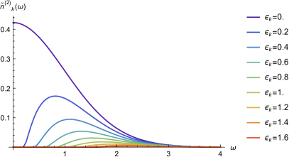
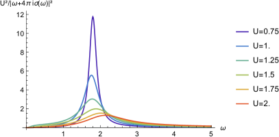
Figure 7: Contributions to the scaled prethermal plateau of $\Delta\langle\hat{n}_{{\bm{k}}\sigma}\rangle_{t>t_{\text{fin}}}/t_{\text{fin}}$ in both second order in the electric field amplitude and interaction with $\bar{\epsilon}_{\bm{k}}$ $=$ $0$ and several $\epsilon_{\bm{k}}$ for the Hubbard model with diagonal field direction (8) subjected to the pump pulse (7) in the limit of long pulse durations $t_{\text{fin}}$, as obtained from the ${\bm{k}}$-dependent factor $\tilde{n}_{{\bm{k}}}^{(2)}(\omega)$ of (27) (left) and the $U$-dependent factor in (29) (right). Here the units are $t^{*}/\hbar$ for frequency, $e^{2}/(\hbar a)$ for $\sigma(\omega)$, $t_{*}$ for energy, $t^{*}/(ea)$ for electric field, and we have chosen $a\cdot|E_{\text{kin}}^{(0)}(0)|$ $=$ $4$ Å $\cdot$ eV, see remarks below (8).

with parameters as given below (8). While the precise response depends on the momentum, the strongest effect will always occur for pump frequencies near the resonance ($\omega_{*}$ $\simeq$ $1.88$). Since the resonance peak becomes larger for small $U$, we conclude that long-lived prethermalization plateaus can be excited by electric fields. Inversely, the value of $U$ could be estimated in principle by locating the resonance frequency for a known band structure. The result (29) corresponds to (2) in the introduction. There, the prefactor $s$ $=$ $1/4$ was split off, which depends on the shape of the envelope. For example, an increase to the maximum amplitude $E$ of the pulse that is steeper than in (7) would result in a larger $s$, which nevertheless remains on the order of unity.

2.4 Prethermal vs. thermal steady states

The prethermalization plateaus (29) for the momentum occupation numbers are proportional to $E^{2}U^{2}$, i.e., they occur in second order in the field and interaction, while in lower orders the momentum occupation always relaxes back to its initial distribution after the pulse. The prethermal value of $n_{{\bm{k}}\sigma}$ could be observed on the one hand by a momentum-resolved probe, such as time-resolved angle-resolved photoemission spectroscopy, as individual momentum occupation numbers, especially close to the Fermi surface, relax rather slowly to their prethermal value and will subsequently exhibit further relaxation to the thermal state. Using optical spectroscopy, on the other hand, it is more difficult to distinguish the prethermalization plateau from the thermal state, i.e., through the time dependence of the conductivity as derived below. This difficulty stems from the fast relaxation of the kinetic energy on the prethermalization time scale $1/t_{*}$, as seen in Figure 4, and it also undergoes no further relaxation since it has then already attained its thermal value in order $U^{2}$. To understand this more quantitatively, we consider the conductivity $\sigma^{\text{pp}}(t,\tau)$ for a probe pulse in linear response when the system is subjected to the pump pulse. For this ‘pump-probe conductivity’ we thus have

$$\sigma^{\text{pp}}(t,\tau) =\sigma^{\text{probe,dia}}(t)+\sigma^{\text{probe,pm}}(t)\,,$$ (30a)

$$\sigma^{\text{pp,dia}}(t) ={e^{2}}\,\langle\hat{H}_{0}^{(2)}\rangle_{t}\,,~{}~{}~{}~{}\sigma^{\text{pp,pm}}(t,\tau)={e^{2}}\,\text{i}\int_{\tau}^{t}\!\text{d}\tau^{\prime}\,\langle\big{[}\hat{H}_{0}^{(1)}(\tau^{\prime}),\hat{H}_{0}^{(1)}(t)\big{]}\rangle_{0}\,.$$ (30b)

Here the Heisenberg operators evolve with the operator $\hat{H}+\delta\hat{H}_{0}(t)$ which describes the pump pulse as given given earlier. After the pulse the diamagnetic contribution $\sigma^{\text{pp}}(t,\tau)$ relaxes similar to the kinetic energy as described above, so that it remains to evaluate the paramagnetic contribution using (11),

$$\langle\big{[}\hat{H}_{0}^{(1)}(\tau^{\prime}),\hat{H}_{0}^{(1)}(t)\big{]}\rangle_{{{0}}} =g^{2}\sum_{l}|V_{0l}|^{2}\big{(}E_{l}^{(1)}\big{)}^{2}\int_{-\infty}^{t}\!\text{d}t_{1}\int_{-\infty}^{\tau^{\prime}}\!\text{d}\tau_{1}\,f(t_{1})f(\tau_{1})\text{e}^{\text{i}\int_{\tau_{1}}^{t_{1}}\!\text{d}t^{\prime}\,(\Delta E_{l}+\delta e_{l}(t^{\prime}))}-\text{c.c.}+O(g^{3})$$

$$=g^{2}\sum_{l}|V_{0l}|^{2}\big{(}E_{l}^{(1)}\big{)}^{2}\text{e}^{\text{i}(t-\tau^{\prime})\Delta E_{l}}\varphi_{l}^{(1)}(t)^{*}\varphi_{l}^{(1)}(\tau^{\prime})-\text{c.c.}+O(g^{3})\,.$$ (31)

We consider $t$ $>$ $t_{\text{fin}}$ and for simplicity assume that pump and probe pulse do not overlap, so that only $\tau$ $>$ $t_{\text{fin}}$ contributes and the upper limit of the integrals can be replaced by $t_{\text{fin}}$,

$$\varphi_{l}^{(1)}(t)=\frac{-1}{\Delta E_{l}}+\text{i}\text{e}^{\text{i}t\Delta E_{l}}h_{l}\,,~{}~{}~{}~{}h_{l}=-\int_{0}^{t_{\text{fin}}}\!\text{d}t_{1}\,\frac{\text{e}^{-\text{i}t_{1}\Delta E_{l}}}{\Delta E_{l}}\text{e}^{\text{i}\int_{t_{1}}^{t_{\text{fin}}}\!\text{d}t^{\prime}\delta e_{l}(t^{\prime})}\delta e_{l}(t_{1})\,,$$ (32)

$$\text{Re}\,\varphi_{l}^{(1)}(t)^{*}\,\text{i}\int_{\tau}^{t}\!\text{d}\tau^{\prime}\text{e}^{\text{i}(t-\tau^{\prime})\Delta E_{l}}\varphi_{l}^{(1)}(\tau^{\prime})=\text{Re}\,\frac{\text{e}^{\text{i}(t-\tau)\Delta E_{l}}-1}{\Delta E_{l}^{3}}+\frac{\text{e}^{\text{i}(t-\tau)\Delta E_{l}}-1}{\Delta E_{l}^{2}}\text{e}^{-\text{i}t\Delta E_{l}}ih_{l}^{*}+\frac{t-\tau}{\Delta E_{l}}\text{e}^{\text{i}t\Delta E_{l}}h_{l}\,.$$ (33)

Here the first term gives the paramagnetic conductivity in equilibrium, while the other terms lead to the transient part of the paramagnetic pump-probe conductivity, which we denote by

$$\Delta\sigma^{\text{pp,pm},(2)}(t,\tau)={e^{2}}\, \int_{0}^{t_{\text{fin}}}\!\text{d}t_{1}\sum_{l}|V_{0l}|^{2}\frac{\big{(}\Delta E_{l}^{(1)}\big{)}^{2}}{\Delta E_{l}^{2}}$$

$$~{}~{}~{}~{}~{}~{}\times\text{e}^{\text{i}\int_{t_{1}}^{t_{\text{fin}}}\!\text{d}t^{\prime}\delta e_{l}(t^{\prime})}\delta e_{l}(t_{1})\Big{(}\text{i}\frac{\text{e}^{\text{i}\tau\Delta E_{l}}-\text{e}^{\text{i}t\Delta E_{l}}}{\Delta E_{l}}-\text{e}^{\text{i}t\Delta E_{l}}(t-\tau)\Big{)}+\text{c.c.}\,.$$ (34)

Since each term contains a factor $\text{e}^{\text{i}t\Delta E_{l}}$ or $\text{e}^{\text{i}\tau\Delta E_{l}}$ this contribution is suppressed for $t$ $>$ $\tau\to\infty$ when integrated over the band energies $E_{l}$. For examples, for the Hubbard model with diagonal field direction $\Delta\sigma^{\text{pp,pm},(2)}(t,\tau)\to 0$ vanishes proportional to a Gaussian $\sim\text{e}^{-\tau^{2}/4}$. As a consequence, the pump-probe conductivity as an integrated quantity is not well-suited to observe the prethermal state, as discussed above.

3 Conclusion

Prethermalized states can in general be generated by time-dependent switching or driving protocols of the interaction or an external field. Here we focused on enveloped electric field pulses which add a time-dependent modulation to the kinetic energy. After the pulse the electronic system relaxes to a prethermal steady state on short timescales $\sim$ $\hbar/bandwidth$. Even for strong fields this behavior is well-described in the leading quadratic orders of interaction and field strength. The response to the pump field will be enhanced for pump pulses near an interaction-dependent resonance frequency which develops due to the field response inside the sample. On the other hand, the details of the pulse shape are found to be less important, as they are merely enter the prefactor $s$ in the leading-order result (2). From an analysis of the real-time conductivity we concluded that momentum-resolved probe techniques are typically necessary to distinguish the prethermal from the thermal state. Our explicit evaluations were performed for a Hubbard model with diagonal field direction in high dimensions, but could be extended to other Hubbard-type systems. For example, the effect of features in the band dispersion or of band degeneracies would be of particular interest. Our general perturbative approach may also be useful to provide input into effective models for later relaxation stages as well as in other contexts.

Acknowledgments

This work was supported in part by Deutsche Forschungsgemeinschaft under project number 107745057 (TRR 80).

Appendix

In this appendix we provide technical details of the evaluations for the Hubbard model with diagonal field direction (8) for the perturbative approach of Section 1.2. The vector potential effectively enters in time arguments of the form $\tau_{1}$ $=$ $\int\text{d}\tau\,\cos A(\tau)$ and $\tau_{2}$ $=$ $\int\text{d}\tau\,\sin A(\tau)$, so that we need to evaluate the following expectation values in the noninteracting ground state $|\Psi_{0}\rangle$

$$\langle\big{[}\hat{D},\big{[}\hat{D}_{I}(\tau_{1},\tau_{2}),\hat{n}_{{\bm{k}}\sigma}\big{]}\big{]}\rangle_{(0)} =2\,\text{Re}\sum_{l}|D_{0l}|^{2}\Delta n_{{\bm{k}},l}\text{e}^{\text{i}\tau_{1}\Delta E_{l}+\text{i}\tau_{2}\Delta\bar{E}_{m}}$$

$$=2\,\text{Re}\sum_{i,\lambda=\pm}\lambda f^{\lambda}_{{\bm{k}}\sigma}(\bm{R}_{i},\tau_{1},\tau_{2})F^{-\lambda}_{\sigma}(\bm{R}_{i},\tau_{1},\tau_{2})\prod\limits_{\lambda^{\prime}=\pm}F^{\lambda^{\prime}}_{\bar{\sigma}}(\bm{R}_{i},\tau_{1},\tau_{2})\,,$$ (35)

$$\text{i}\langle\big{[}\hat{D},\hat{D}_{I}(\tau_{1},\tau_{2})\big{]}\rangle_{(0)} =2\,\text{Re}\sum_{l}|D_{0l}|^{2}\,\text{i}\,\text{e}^{\text{i}\tau_{1}\Delta E_{l}+\text{i}\tau_{2}\Delta\bar{E}_{m}}$$

$$=\,\text{Re}\,\text{i}\sum_{i}\prod\limits_{\lambda=\pm}F^{\lambda}_{\bar{\sigma}}(\bm{R}_{i},\tau_{1},\tau_{2})F^{\lambda}_{\sigma}(\bm{R}_{i},\tau_{1},\tau_{2})\,,$$ (36)

in terms of $D_{nm}$ $=$ $\langle\Psi_{n}|\hat{n}^{\phantom{\dagger}}_{i\uparrow}\hat{n}^{\phantom{\dagger}}_{i\downarrow}|\Psi_{m}\rangle$, $\delta\hat{\bar{H}}_{0}|\Psi_{l}\rangle$ $=$ $\bar{E}_{l}|\Psi_{l}\rangle$ $\Delta\bar{E}_{l}$ $=$ $\bar{E}_{l}-\bar{E}_{0}$, and the functions ($\lambda$ $=$ $\pm$)

$$f^{\lambda}_{{\bm{k}}\sigma}(\bm{R}_{i},\tau_{1},\tau_{2})=\text{e}^{-\text{i}(\bm{R}_{i}\cdot{\bm{k}}+\tau_{1}\epsilon_{{\bm{k}}}+\tau_{2}\bar{\epsilon}_{{\bm{k}}})}\langle\delta_{\lambda+}+\lambda\hat{n}_{{\bm{k}}\sigma}\rangle_{(0)}\,,~{}~{}~{}~{}~{}~{}F^{\lambda}_{\sigma}(\bm{R}_{i},\tau_{1},\tau_{2})=\frac{1}{L}\sum_{{\bm{k}}}f^{\lambda}_{{\bm{k}}\sigma}(\bm{R}_{i},\tau_{1},\tau_{2})\,.$$ (37)

In the limit of high dimensions only the local term $\bm{R}_{i}$ $=$ $\bm{0}$ contributes, leading to integrals over the density of states (8c),

$$F^{\lambda}_{\sigma}(\tau_{1},\tau_{2}) =\int\text{d}\epsilon\int\text{d}\bar{\epsilon}\,\rho(\epsilon,\bar{\epsilon})\,\text{e}^{-\lambda\text{i}(\tau_{1}\epsilon+\tau_{2}\bar{\epsilon})}\langle\delta_{\lambda+}+\lambda\hat{n}_{\epsilon\bar{\epsilon}\sigma}\rangle_{(0)}$$

$$=F(\tau_{1},\tau_{2}) =\int_{0}^{\infty}\text{d}\epsilon\frac{\text{e}^{-\epsilon^{2}+\text{i}\epsilon\tau_{1}}}{\sqrt{\pi}}\,\int_{-\infty}^{\infty}\text{d}\bar{\epsilon}\frac{\text{e}^{-\bar{\epsilon}^{2}+\text{i}\bar{\epsilon}\tau_{2}}}{\sqrt{\pi}}\,,$$ (38)

where the second line, independent of $\lambda$ and $\sigma$, applies for the paramagnetic ground state of the half-filled band. For the expectation values

$$D^{(1)}(t)=\sum_{l}|D_{0l}|^{2}\varphi_{l}^{(1)}(t)+\text{c.c.}\,,~{}~{}~{}~{}n_{{\bm{k}}\sigma}^{(2)}(t)=\sum_{l}|D_{0l}|^{2}\Delta n_{{\bm{k}},l}\varphi_{l}^{(2)}(t)\,,$$ (39)

we require $\varphi^{(1)}_{l}(t)$ and $\varphi^{(2)}_{l}(t)$ from (11c) and (12b), which involve $\delta e_{l}(t_{2})$ $=$ $\Delta E_{l}\,(\cos A(t_{2})-1)+\Delta\bar{E}_{l}\,\sin A(t_{2})$. We are left with powers of $\Delta E_{l}$ and $\Delta\bar{E}_{l}$, which we rewrite as

$$(\Delta E_{l})^{n_{1}}(\Delta\bar{E}_{l})^{n_{2}}\text{e}^{\text{i}\tau_{1}\Delta E_{l}+\text{i}\tau_{2}\Delta\bar{E}_{l}}=\Big{(}\frac{\partial}{\partial\,\text{i}\tau_{1}}\Big{)}^{n_{1}}\,\Big{(}\frac{\partial}{\partial\,\text{i}\tau_{2}}\Big{)}^{n_{2}}\,\text{e}^{\text{i}\tau_{1}\Delta E_{l}+\text{i}\tau_{2}\Delta\bar{E}_{l}}\,,$$ (40)

with exponents $n_{1}\in\{-2,-1,0,1\}$ and $n_{2}\in\{0,1,2\}$. Then the sum over states can be performed, resulting again integrals $F(\tau_{1},\tau_{2})$ over the density of states. Its differentiation is straightforward, while for positive exponents the integrations (with appropriate integration limits) are best simplified by another transformation. Consider first the functions appearing in $D^{(1)}(t)$,

$$F(\tau_{1},\tau_{2})^{m} =\bigg{(}\int_{-\infty}^{\infty}\text{d}\bar{\epsilon}\frac{\text{e}^{-\bar{\epsilon}^{2}+\text{i}\bar{\epsilon}\tau_{2}}}{\sqrt{\pi}}\bigg{)}^{m}\int_{0}^{\infty}\text{d}\epsilon_{1}\ldots\int_{0}^{\infty}\text{d}\epsilon_{m}\frac{\text{e}^{-\sum_{l=1}^{m}\epsilon_{l}^{2}+\text{i}\epsilon_{l}\tau_{1}}}{\sqrt{\pi^{m}}}$$ (41)

$$=\text{e}^{-\frac{m\tau_{2}^{2}}{4}}\int_{0}^{\infty}\text{d}\epsilon_{0}\,\frac{\text{e}^{\text{i}\tau_{1}\epsilon_{0}}}{\sqrt{\pi^{m}}}\int_{0}^{\infty}\text{d}\epsilon_{1}\ldots\int_{0}^{\infty}\text{d}\epsilon_{m}\,\delta(\epsilon_{0}-\sum_{l=1}^{m}\epsilon_{l})\text{e}^{-\sum_{l=1}^{m}\epsilon_{l}^{2}}\,,$$ (42)

which can be expressed in terms of a weight function

$$a_{n}(b) =\int_{0}^{\infty}\text{d}x_{1}\ldots\int_{0}^{\infty}\text{d}x_{n}\,\delta(1-\sum_{i=1}^{n}x_{i})\delta(b-\sum_{j=1}^{n}x_{j}^{2})\,.$$ (43)

Integrating $m-1$ times we obtain

$$\Big{(}\frac{\partial}{\partial\,\text{i}\tau_{1}}\Big{)}^{1-m}\,F(\tau_{1},\tau_{2})^{m} =\text{e}^{-\frac{m\tau_{2}^{2}}{4}}\int_{0}^{\infty}\text{d}b\int_{0}^{\infty}\text{d}\epsilon_{0}\,\frac{\text{e}^{\text{i}\tau_{1}\epsilon_{0}-b\epsilon_{0}^{2}}}{\sqrt{\pi^{m}}}a_{m}(b)\,,$$ (44)

$$\Big{(}\frac{\partial}{\partial\,\text{i}\tau_{1}}\Big{)}^{1-m}\,F(\tau_{1},\tau_{2})^{m} =\text{e}^{-\frac{m\tau_{2}^{2}}{4}}\int_{\frac{1}{m}}^{1}\text{d}b\,\frac{a_{m}(b)}{\sqrt{b\pi^{m}}}\Big{(}\frac{\sqrt{\pi}}{2}\text{e}^{-\frac{\tau_{1}^{2}}{4b}}+\text{i}\,\text{D}_{+}(\tfrac{\tau_{1}}{2\sqrt{b}})\Big{)}\,,$$ (45)

where the Dawson function $\text{D}_{+}(x)$ was defined in (16c). We need only the cases $n$ $=$ $3,4$, for which [36]

$$a_{3}(b) =\begin{cases}\dfrac{\pi}{\sqrt{3}}&\text{if~{}}\frac{1}{3}\leq b\leq\frac{1}{2},\\[4.30554pt] \dfrac{\pi}{\sqrt{3}}-\sqrt{3}\arccos\dfrac{1}{\sqrt{6b-2}}&\text{if~{}}\frac{1}{2}\leq b\leq 1,\\[4.30554pt] 0&\text{otherwise,}\end{cases}$$ (46)

$$a_{4}(b) =\begin{cases}\pi\sqrt{b-\frac{1}{4}}&\text{if~{}}\frac{1}{4}<b<\frac{1}{3},\\ \dfrac{\pi}{\sqrt{3}}-\pi\sqrt{b-\frac{1}{4}}&\text{if~{}}\frac{1}{3}<b<\frac{1}{2},\\ \sqrt{3}\,\arcsin\dfrac{1}{\sqrt{6b-2}}+3\sqrt{b-\frac{1}{4}}\,\arcsin\dfrac{\sqrt{1-6b+8b^{2}}}{3b-1}-\dfrac{\pi}{2\sqrt{3}}-\pi\sqrt{b-\frac{1}{4}}&\text{if~{}}\frac{1}{2}<b<1,\\ 0&\text{otherwise.}\end{cases}\!\!\!\!\!\!$$ (47)

Integrations are thus avoided for ${m-1+n_{1}\geq 0}$ with $m\in\{3,4\}$, except for one final numerical integration over $b$. For $n_{{\bm{k}}\sigma}^{(2)}(t)$, on the other hand, an integration over $\epsilon_{0}$ also remains. In this case we need (for $\epsilon>0$)

$$\text{e}^{\text{i}\tau_{1}\epsilon}F(\tau_{1},\tau_{2})^{3} =\text{e}^{-\frac{3\tau_{2}^{2}}{4}}\int_{\epsilon}^{\infty}\text{d}\epsilon_{0}\,\frac{\text{e}^{\text{i}\tau_{1}\epsilon}}{\sqrt{\pi^{3}}}\int_{0}^{\infty}\text{d}\epsilon_{1}\int_{0}^{\infty}\text{d}\epsilon_{2}\int_{0}^{\infty}\text{d}\epsilon_{3}\,\delta(\epsilon_{0}-\epsilon-\epsilon_{1}-\epsilon_{2}-\epsilon_{3})\text{e}^{-\epsilon_{1}^{2}-\epsilon_{2}^{2}-\epsilon_{3}^{2}}$$

$$=\text{e}^{-\frac{3\tau_{2}^{2}}{4}}\int_{\epsilon}^{\infty}\text{d}\epsilon_{0}\,\epsilon_{0}^{2}\int_{0}^{\infty}\text{d}b\,\frac{\text{e}^{\text{i}\tau_{1}\epsilon-b\epsilon_{0}^{2}}}{\sqrt{\pi^{3}}}\,a_{3}\Big{(}\frac{b\epsilon_{0}^{2}}{(\epsilon_{0}-\epsilon)^{2}}\Big{)}\,.$$ (48)

Integrating twice and rearranging the integrals we arrive at

$$\Big{(}\frac{\partial}{\partial\,\text{i}\tau_{1}}\Big{)}^{-2}\,\text{e}^{\text{i}\tau_{1}\epsilon}F(\tau_{1},\tau_{2})^{3}=\text{e}^{-\frac{3\tau_{2}^{2}}{4}}\int_{\frac{1}{3}}^{1}\text{d}b\,a_{3}(b)\int_{\epsilon}^{\infty}\frac{\text{d}\epsilon_{0}}{\epsilon_{0}^{2}}\,(\epsilon_{0}-\epsilon)^{2}\,\frac{\text{e}^{\text{i}\tau_{1}\epsilon_{0}-b\epsilon_{0}^{2}}}{\sqrt{\pi^{3}}}\,,$$ (49)

which can be differentiated analytically with respect to $\tau_{1}$ and $\tau_{2}$ as needed, leaving numerical integrations over $b$, $t_{1}$, and $t_{2}$. In the limit $\epsilon\to 0$, we recover the previous result. For $\epsilon$ $>$ $0$ we integrate numerically over $\epsilon_{0}$ as well.

References

- [1] D. N. Basov, R. D. Averitt, D. Hsieh, Nature Materials 2017, 16 1077.
- [2] Y. Wang, M. Claassen, C. D. Pemmaraju, C. Jia, B. Moritz, T. P. Devereaux, Nature Rev. Materials 2018, 3 312.
- [3] A. de la Torre, D. M. Kennes, M. Claassen, S. Gerber, J. W. McIver, M. A. Sentef, Rev. Mod. Phys. 2021, 93 041002.
- [4] H. Aoki, N. Tsuji, M. Eckstein, M. Kollar, T. Oka, P. Werner, Rev. Mod. Phys. 2014, 86 779.
- [5] K. Yonemitsu, K. Nasu, J. Phys. Soc. Jpn. 2006, 75 011008.
- [6] Y. H. Wang, H. Steinberg, P. Jarillo-Herrero, N. Gedik, Science 2013, 342 453.
- [7] M. Bukov, L. D’Alessio, A. Polkovnikov, Adv. Phys. 2015, 64 139.
- [8] E. Canovi, M. Kollar, M. Eckstein, Phys. Rev. E 2016, 93 012130.
- [9] A. Herrmann, Y. Murakami, M. Eckstein, P. Werner, EPL 2017, 120 57001.
- [10] H. Hübener, M. A. Sentef, U. De Giovannini, A. F. Kemper, A. Rubio, Nature Communications 2017, 8 13940.
- [11] J. Tindall, F. Schlawin, M. A. Sentef, D. Jaksch, Phys. Rev. B 2021, 103 035146.
- [12] J. H. Mentink, K. Balzer, M. Eckstein, Nature Communications 2015, 6 6708.
- [13] R. V. Mikhaylovskiy, E. Hendry, A. Secchi, J. H. Mentink, M. Eckstein, A. Wu, R. V. Pisarev, V. V. Kruglyak, M. I. Katsnelson, T. Rasing, A. V. Kimel, Nature Communications 2015, 6 8190.
- [14] S. Braun, J. P. Ronzheimer, M. Schreiber, S. S. Hodgman, T. Rom, I. Bloch, U. Schneider, Science 2013, 339 52.
- [15] J. Berges, Nonequilibrium quantum fields: from cold atoms to cosmology, Oxford University Press, 2016.
- [16] M. Moeckel, S. Kehrein, Phys. Rev. Lett. 2008, 100 175702.
- [17] M. Eckstein, M. Kollar, P. Werner, Phys. Rev. Lett. 2009, 103 056403.
- [18] B. Bertini, F. H. Essler, S. Groha, N. J. Robinson, Phys. Rev. Lett. 2015, 115 180601.
- [19] J. Berges, A. Rothkopf, J. Schmidt, Phys. Rev. Lett. 2008, 101 041603.
- [20] M. Heyl, Rep. Prog. Phys. 2018, 81 054001.
- [21] H. J. Zeiger, J. Vidal, T. K. Cheng, E. P. Ippen, G. Dresselhaus, M. S. Dresselhaus, Phys. Rev. B 1992, 45 768.
- [22] L. Yang, G. Rohde, T. Rohwer, A. Stange, K. Hanff, C. Sohrt, L. Rettig, R. Cortés, F. Chen, D. Feng, T. Wolf, B. Kamble, I. Eremin, T. Popmintchev, M. Murnane, H. Kapteyn, L. Kipp, J. Fink, M. Bauer, U. Bovensiepen, K. Rossnagel, Phys. Rev. Lett. 2014, 112 207001.
- [23] V. Turkowski, J. K. Freericks, Phys. Rev. B 2005, 71 085104.
- [24] J. Li, M. Eckstein, Phys. Rev. B 2021, 103 045133.
- [25] M. Schüler, J. A. Marks, Y. Murakami, C. Jia, T. P. Devereaux, Phys. Rev. B 2021, 103 155409.
- [26] L. Erdős, M. Salmhofer, H.-T. Yau, J. Stat. Phys. 2004, 116 367.
- [27] F. Schmitt, P. S. Kirchmann, U. Bovensiepen, R. G. Moore, L. Rettig, M. Krenz, J.-H. Chu, N. Ru, L. Perfetti, D. H. Lu, M. Wolf, I. R. Fisher, Z.-X. Shen, Science 2008, 321 1649.
- [28] M. Wais, M. Eckstein, R. Fischer, P. Werner, M. Battiato, K. Held, Phys. Rev. B 2018, 98 134312.
- [29] T. Mori, T. N. Ikeda, E. Kaminishi, M. Ueda, J. Phys. B: At. Mol. Opt. Phys. 2018, 51 112001.
- [30] A. Picano, J. Li, M. Eckstein, Phys. Rev. B 2021, 104 085108.
- [31] J. Skolimowski, A. Amaricci, M. Fabrizio, Phys. Rev. B 2020, 101 121104.
- [32] D. J. Scalapino, S. R. White, S. Zhang, Phys. Rev. B 1993, 47 7995.
- [33] W. Metzner, D. Vollhardt, Phys. Rev. Lett. 1989, 62 324.
- [34] A. Georges, G. Kotliar, W. Krauth, M. J. Rozenberg, Rev. Mod. Phys. 1996, 68 13.
- [35] G. Kotliar, S. Y. Savrasov, K. Haule, V. S. Oudovenko, O. Parcollet, C. A. Marianetti, Rev. Mod. Phys. 2006, 78 865.
- [36] M. Alexander, M. Kollar, (unpublished).