Impact of Atrial Fibrillation on Left Atrium Haemodynamics: A Computational Fluid Dynamics Study

Abstract

We analyse the haemodynamics of the left atrium, highlighting differences between healthy individuals and patients affected by atrial fibrillation. The computational study is based on patient-specific geometries of the left atria to simulate blood flow dynamics. We design a novel procedure to compute the boundary data for the 3D haemodynamic simulations, which are particularly useful in absence of data from clinical measurements. With this aim, we introduce a parametric definition of atrial displacement, and we use a closed-loop lumped parameter model of the whole cardiovascular circulation conveniently tuned on the basis of the patient’s characteristics. We evaluate several fluid dynamics indicators for atrial haemodynamics, validating our numerical results in terms of clinical measurements; we investigate the impact of geometric and clinical characteristics on the risk of thrombosis. To highlight the correlation of thrombus formation with atrial fibrillation, according to medical evidence, we propose a novel indicator: age stasis. It arises from the combination of Eulerian and Lagrangian quantities. This indicator identifies regions where slow flow cannot properly rinse the chamber, accumulating stale blood particles, and creating optimal conditions for clots formation.

1 Introduction

Atrial fibrillation (AF) is the most common cardiac electric dysfunction worldwide [1]. The irregular electrical impulses of this pathology cause a reduced atrial contraction and thus a smaller blood ejection. According to the European Society of Cardiology (ESC), in 2016, 7.6 million people aged 65 and over were affected by AF in the European Union. Figures would increase up to 14.4 million within 2060 [1].

In terms of pathology severity, AF is divided into three categories: paroxysmal AF is an episode that typically self-terminates within seven days; persistent AF requires termination by pharmacological or direct-current electric cardioversion; permanent AF is irreversible to sinus rhythm [2, 3, 4]. Persistent AF can cause long-term remodeling of the atrial chambers, increasing atrial volume and causing thrombogenic formation in the Left Atrial Appendage (LAA) [5, 6]. Two centuries ago, “Virchow’s triad” was defined to denote the three main factors contributing to the risk of thrombosis: endothelial injuries, hypercoagulability, and blood stasis [7]. The correlation between these elements and AF is nowadays established [5, 8].

In this paper, we investigate the effects of AF on instantaneous cardiac haemodynamics. Cardiac blood flow analysis is commonly assessed using both imaging and experimental techniques. For example, 4D flow MRI [9], one of the most advanced imaging techniques, allows the detection of a time-dependent blood flow fields [10], the estimation of haemodynamic parameters such as flow stasis, mean velocity [11], and particle tracking. However, the resolution provided by 4D flow MRI might not be enough to accurately catch the complexity of cardiac flows and their transitional effects: the formation of shear layers, small vortices, and their interactions [12, 13, 14, 15, 16]. For this reason, in-silico simulations of the heart, often combined with medical images, stand as a valuable tool for a more accurate description of blood flows, using haemodynamic indicators as the wall shear stress (WSS) [17, 18, 19, 20].

Literature abounds with CFD studies of human atria under AF, both for idealized [21, 22] and patient-specific geometries [23, 24, 25, 26, 27, 28, 29, 30]. Concerning the numerical approach, in [24], CFD simulations were performed without the application of a turbulence model; in [25, 26], the LA haemodynamics is modelled via the Navier-Stokes (NS) equations in Arbitrary Lagrangian-Eulerian (ALE) formulation; the Variational Multiscale Large Eddy Simulation (VMS-LES) method [31] is used to account for possible transitional-to-turbulent flows. Moreover, a comparison is made considering the differences derived from applying or not an LES model in AF conditions in [19]. They numerically demonstrated that the absence of a turbulence model is acceptable in AF conditions.

Due to the relevance of LAA in thrombus formation, many studies investigate how the geometrical morphology of this region of the LA affects blood flow [32, 33, 34, 35, 36, 37, 38]. These works suggest the existence of a strong correlation between LAA morphology and thromboembolic risk; moreover, AF aggravates this danger.

In this paper, we consider patient-specific geometries of the LA and we carry out CFD simulations that provide a complete characterisation of blood flow under physiological and pathological conditions. In particular, the atrial geometries we have available [39, 40] are scanned at the end of diastole only [41]. Thus, we cannot derive any clinical information in terms of boundary pressures, flowrates, and displacement. Thus, a 0D closed-loop circulation model [42] serves as input to prescribe boundary conditions to the 3D CFD problem, by employing a “one-way” 3D-0D coupling scheme. More precisely, we customize the closed-loop circulation model with the available patient-specific data to get transient data that we prescribe on the boundary of the CFD domain. Specifically, to simulate AF conditions, we conveniently tune the circulation model as explained in [43]. Thus, the proposed procedure allows to carry out numerical simulations also when time dependent patient-specific data are not available. Moreover, since fluxes and displacement are coming from the same circulation model, the mass conservation property of the 0D closed-loop model is naturally encoded in the 3D boundary conditions. This guarantees to satisfy the compatibility condition of the NS equations [44] that are required for the well-posedness of the problem. On the contrary, fluxes and displacements obtained from measurements not related to the same patient would not guarantee this property, thus affecting the meaningfulness of the corresponding numerical solution.

Contextually, we tune additional model parameters to account for the volumetric constraints given by the patient-specific atrial geometries. We also used this calibration process to obtain meaningful Left Atrial Ejection Fractions (LAEF). Similarly to [45, 46], we use a parametric displacement combined with patient-specific geometries to fill the lack of information on the chamber displacement. Starting from the analytical formulation in [45], that prescribed a movement directed towards the centre of mass of LA, we modify it to capture a more realistic displacement of the LAA and to match the volume variations with the physiological or pathological values of the Left Atrial Appendage Ejection Fraction (LAAEF) [47]. We generate a displacement field that embodies patient-specific constraints to obtain a more physiological motion of the atrial chamber and of its auricle. We believe that this is essential to estimate the risk of thrombosis in the LA, considering that LAA is the area where thrombi formation begins [5]. Furthermore, a parametric displacement allows us to simulate different levels of severity of AF according to the clinical situation of the patients by conveniently changing the parameters involved in the displacement definition. However, this model relies on a number of assumptions that we cannot entirely validate by carrying out a direct comparison between our displacement and some in-vivo recordings, since kinematic data are not available. Thus, in order to assess the correctness of our numerical results, we compare a numbers of in-silico values with biomarkers available in literature that are acquired in healthy and pathological patients. We show that the computed values always lie in the given ranges. Furthermore, we highlight that the methodology we employ aims to carry out LA haemodynamic simulations in both physiologic and AF conditions, overcoming the problem of missing data, and with a contained computational cost.

In many works on atrial haemodynamic simulations, the effects of the mitral valve (MV) are mimicked by employing switching boundary conditions [25, 26, 22, 24]. Differently, in this paper, we model the effect of the MV on the fluid flow through the Resistive Immersed Implicit Surface (RIIS) method [48, 18, 49]. Furthermore, we prescribe valvular opening and closing times that are consistent with clinical findings, overcoming the classical oversimplification of an instantaneous switch of the valvular status [25, 26, 22, 24]. To the best of our knowledge, the only work in the literature that simulates left atrial haemodynamics considering the presence of MV is [50], where a fluid-structure interaction model is employed to perform an advanced analysis of the valvular motion.

Finally, we analyze some haemodynamic indicators both from Eulerian and Lagrangian perspectives. The Eulerian indicators are directly derived from the results of the NS simulations. Differently, the Lagrangian ones are obtained by simulating the red blood cells motion in the atrial chamber. We consider particles like tracers (their presence does not influence the blood flow) [17], and, taking advantage of the kinetic theory development for particles transport [51], we derive some Lagrangian fields as mean age and washout of the blood [52]. The combination of these two approaches has been successfully applied in the literature to analyse blood flow in ventricles [17, 53]. In this paper, for the first time, we propose a new hybrid indicator, that we call age stasis, which is defined as the product between a Lagrangian term and an Eulerian one. It detects regions with high thrombotic risk, where stagnant flow and high blood mean age subsist at the same time. As a matter of fact, the coexistence of these two situations denotes a high risk of blood clots formation. Furthermore, we derive a dimensionless indicator that estimates the percentage of volume associated with a higher risk and exploring its correlation with the AF pathology. This allows to carry out comparisons among different patients in terms of a single, synthetic indicator.

This paper is organised as follows: we present the mathematical models and methods in Section 2. Finally, in Section 3, we present the numerical results of both the $0D-$model and CFD simulation. In particular, in Section 3.4, we propose our haemodynamic indicator. The discussion of the results is reported in Section 4. Eventually, conclusions are drawn in Section 5.

2 Methods

In this section, we introduce the methods we employ to carry out CFD simulations. Particularly, in Section 2.1, we introduce the mathematical models and numerical methods. Section 2.2 is devoted to the description of boundary conditions obtained via the lumped-parameter circulation model and the parametrization of the atrial displacement. Section 2.3 concerns the setup of the CFD simulations.

2.1 Mathematical models and numerical methods for left atrial haemodynamics

This section introduces the mathematical models to describe the fluid dynamics in LA. To carry out the simulations, we use the medical images that were obtained by [41]. The derived endocardial geometries are openly accessible from the supplementary material of [39, 40]. Data are scanned at the time of end diastole only. Thus, we do not have any knowledge in terms of displacement field, boundary flowrates and boundary pressures.

Let $\Omega_{t}$ be the fluid domain at a specific time instant $t\in(0,T)$ (current configuration) and let $\partial\Omega_{t}$ be its boundary, being $T$ the final time. To take into account the moving reference framework, we employ the ALE formulation [54]. Let $\widehat{\Omega}\subset\mathbb{R}^{3}$ be the LA domain in its reference configuration, as displayed in Figure 1. We define the ALE map $\boldsymbol{\mathcal{A}}_{t}$, which associates at each point of the reference configuration $\widehat{\boldsymbol{x}}$ the corresponding point in the actual one $\boldsymbol{x}$, such that $\boldsymbol{\mathcal{A}}_{t}:\widehat{\Omega}\rightarrow\Omega_{t}$ and $\boldsymbol{x}=\boldsymbol{\mathcal{A}}_{t}(\widehat{\boldsymbol{x}})=\widehat{\boldsymbol{x}}+\widehat{\boldsymbol{d}}(\widehat{\boldsymbol{x}},t)$, being $\widehat{\boldsymbol{d}}$ the displacement with respect to the reference configuration.

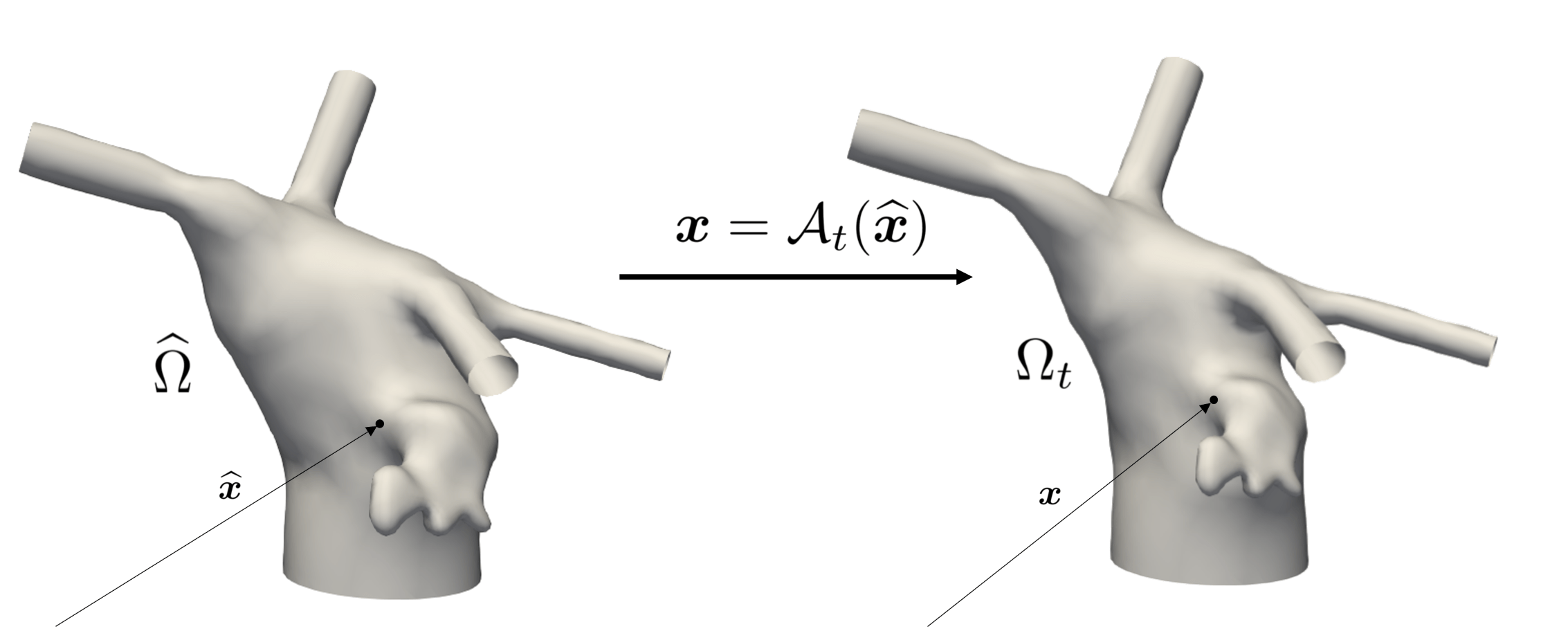
Figure 1: Left atrial domain in reference configuration $\widehat{\Omega}$ (left), in current configuration $\Omega_{t}$ (right), and the ALE map $\boldsymbol{x}=\boldsymbol{\mathcal{A}}_{t}(\widehat{\boldsymbol{x}})$.

As shown in Figure 2, we split the boundary as $\partial\Omega_{t}=\Gamma_{t}^{\mathrm{W}}\cup\Gamma^{\mathrm{MV}}\cup\Big{(}\bigcup_{j=1}^{4}\Gamma^{\mathrm{PV}_{j}}\Big{)}$, being $\Gamma_{t}^{\mathrm{W}}$ the endocardial wall, $\Gamma^{\mathrm{PV}_{j}}$ the $j$-th pulmonary vein inlet section, with $j=1,\dots,4$, and $\Gamma^{\mathrm{MV}}$ the outlet section downstream of the MV. For the sake of simplicity, we consider the inlet and outlet sections to be fixed, neglecting hence the time dependency in the notation.

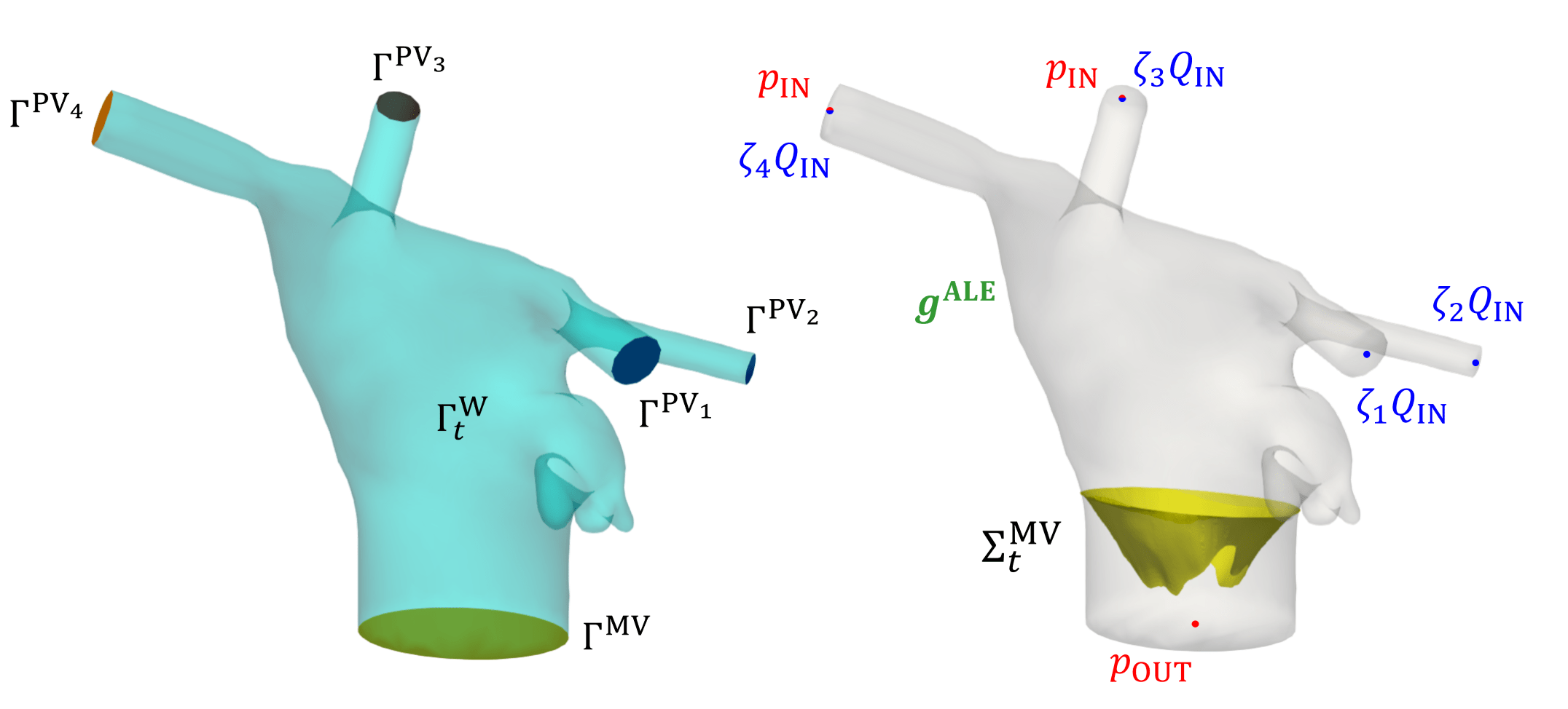
Figure 2: LA domain with details on the boundaries (left), and with the representation of the MV surface $\Sigma^{\mathrm{MV}}_{t}$ and of the boundary data that we prescribe (right).

Should we know a boundary velocity $\boldsymbol{g}^{\mathrm{ALE}}:\partial\Omega_{t}\times(0,T)\rightarrow\mathbb{R}^{3}$, we recover the ALE velocity $\boldsymbol{u}^{\mathrm{ALE}}:\Omega_{t}\times(0,T)\rightarrow\mathbb{R}^{3}$ by means of the following harmonic extension problem:

$$\begin{cases}-\Delta\boldsymbol{u}^{\mathrm{ALE}}=\boldsymbol{0}&\mathrm{in}\;\Omega_{t}\times(0,T),\\ \boldsymbol{u}^{\mathrm{ALE}}=\boldsymbol{g}^{\mathrm{ALE}}&\mathrm{on}\;\partial\Omega_{t}\times(0,T),\\ \end{cases}$$ (1)

which allows regaining displacement as: $\boldsymbol{d}(\boldsymbol{x},t)=\int_{0}^{t}\boldsymbol{u}^{\mathrm{ALE}}(\boldsymbol{x},\tau)d\tau$.

In the heart chambers, it is assumed that blood behaves as a Newtonian, incompressible, and homogeneous fluid [55, 56]. Under this assumption, the Cauchy’s stress tensor is defined as $\boldsymbol{\sigma}(\boldsymbol{u},p)=-p\mathbf{I}+\mu\left(\nabla\boldsymbol{u}+(\nabla\boldsymbol{u})^{\top}\right)$, where $\boldsymbol{u}:\Omega_{t}\times(0,T)\rightarrow\mathbb{R}^{3}$ is the fluid velocity field, $p:\Omega_{t}\times(0,T)\rightarrow\mathbb{R}$ the pressure field and $\mu$ the dynamic viscosity. Then, the fluid dynamics equations read:

$$\begin{cases}\rho\left(\dfrac{\widehat{\partial}\boldsymbol{u}}{\widehat{\partial}t}+((\boldsymbol{u}-\boldsymbol{u}^{\mathrm{ALE}})\cdot\nabla)\boldsymbol{u}\right)-\nabla\cdot\boldsymbol{\sigma}(\boldsymbol{u},p)+\dfrac{R}{\varepsilon}\delta_{\varepsilon}^{\Sigma}(\varphi)(\boldsymbol{u}-\boldsymbol{u}_{\Sigma})=\boldsymbol{0}&\mathrm{in}\;\Omega_{t}\times(0,T),\\ \nabla\cdot\boldsymbol{u}=0&\mathrm{in}\;\Omega_{t}\times(0,T).\end{cases}$$ (2)

To account for the presence of the MV in the fluid, in Equation 2, we use the Resistive Immersed Implicit Surface (RIIS) method, proposed by [48] for the simulation of the aortic valve, and extended to the ALE case in [18]. With the RIIS method, we identify the MV as an immersed surface described by the level set function $\varphi:\Omega_{t}\rightarrow\mathbb{R}$ as $\Sigma^{\mathrm{MV}}_{t}=\{\boldsymbol{x}\in\Omega_{t}:\;\varphi(\boldsymbol{x})=0\}$. Moreover, $\varepsilon$ is a parameter representing the half-thickness of the MV leaflets, $R$ the valve resistance, and $\delta^{\Sigma}_{\varepsilon}$ is the smooth Dirac delta function defined as in [48]. The valve velocity is set to be null, using the quasi-static approximation $(\boldsymbol{u}_{\Sigma}=\boldsymbol{0})$ [18, 49].

2.1.1 Boundary and initial conditions

We apply a nonhomogeneous Dirichlet no-slip condition $\boldsymbol{u}=\boldsymbol{g}^{\mathrm{ALE}}$ on the endocardial wall $\Gamma_{t}^{\mathrm{W}}$; the boundary datum $\boldsymbol{g}^{\mathrm{ALE}}$ is obtained as presented in Section 2.2. On the MV section $\Gamma^{\mathrm{MV}}$, we impose an outflow Neumann boundary condition considering as mean stress value $p_{\mathrm{OUT}}$. We consider heartbeat and diastole duration $T_{\mathrm{HB}}$ and $T_{\mathrm{d}}$, respectively.

Regarding the inlet sections $\Gamma^{\mathrm{PV}}_{j}$, we use a Dirichlet boundary condition for all veins in the diastolic phase $(0,T_{\mathrm{d}}]$, imposing an inlet flux $Q_{\mathrm{IN}}$. However, in principle, this would be a defective condition, since it prescribes only one scalar function through the section and not the overall velocity field [55]. A possible way to fill this gap is to prescribe a parabolic velocity profile to complete the information. In the systolic phase of the heartbeat $(T_{\mathrm{d}},T_{\mathrm{HB}}]$, the closed MV would not allow a correct estimate of the atrial pressure without imposition of a Neumann condition on some veins. For this reason, we switch the boundary conditions in two inlet sections, by prescribing the mean pressure value $p_{\mathrm{IN}}$, as done in [55]. For the switching BCs, following arguments of [57], we set the same pressures in vessels of the same size. Thus, we choose the two veins being characterized by the most similar cross-section areas. Moreover, to (weakly) penalise the reverse flow, we introduce backflow stabilization in all the Neumann boundaries to avoid numerical instabilities [58].

We denote by $\tilde{R}_{j}$ the radius of the $j-$th inlet section; $r(\boldsymbol{x})=|\boldsymbol{x}|_{2}$ is the radial coordinate of the point $\boldsymbol{x}\in\Gamma^{\mathrm{PV}_{j}}$, $|\cdot|_{2}:\mathbb{R}^{3}\rightarrow\mathbb{R}$ being the Euclidean norm. To distribute the inlet flow in veins having different cross sections, we introduce a flow repartition factor associated with the $j$–th vein. We compute it proportionally to the inlet area as:

$$\zeta_{j}=\dfrac{|\Gamma^{\mathrm{PV}_{j}}|}{\sum_{k=1}^{4}|\Gamma^{\mathrm{PV}_{k}}|}.$$ (3)

The way we compute the boundary conditions $Q_{\mathrm{IN}}$, $p_{\mathrm{IN}}$, $p_{\mathrm{OUT}}$ and $\boldsymbol{g}^{\mathrm{ALE}}$ is discussed in Section 2.2.

Moreover, we consider a null initial condition $\boldsymbol{u}(\boldsymbol{x},0)=\boldsymbol{0}$. The NS-ALE-RIIS equations with the boundary and initial conditions to simulate the LA haemodynamics read:

for every $t>0$, find $\boldsymbol{u}:\Omega_{t}\times(0,T)\rightarrow\mathbb{R}^{3}$ and $p:\Omega_{t}\times(0,T)\rightarrow\mathbb{R}$:

$$\begin{cases}\rho\left(\dfrac{\widehat{\partial}\boldsymbol{u}}{\widehat{\partial}t}+((\boldsymbol{u}-\boldsymbol{u}^{\mathrm{ALE}})\cdot\nabla)\boldsymbol{u}\right)-\nabla\cdot\boldsymbol{\sigma}(\boldsymbol{u},p)+\dfrac{R}{\varepsilon}\delta_{\varepsilon}^{\Sigma}(\varphi)\boldsymbol{u}=\boldsymbol{0}&\mathrm{in}\;\Omega_{t}\times(0,T_{\mathrm{HB}}],\\ \nabla\cdot\boldsymbol{u}=0&\mathrm{in}\;\Omega_{t}\times(0,T_{\mathrm{HB}}],\\ \boldsymbol{u}=\boldsymbol{g}^{\mathrm{ALE}}&\mathrm{on}\;\Gamma^{\mathrm{W}}_{t}\times(0,T_{\mathrm{HB}}],\\ \boldsymbol{u}=-2\zeta_{k}\dfrac{Q_{\mathrm{IN}}}{|\Gamma^{\mathrm{PV}_{k}}|}\Big{(}1-\dfrac{r^{2}}{\tilde{R}_{k}^{2}}\Big{)}\boldsymbol{n}_{k}&\mathrm{on}\;\Gamma^{\mathrm{PV}_{k}}\times(0,T_{\mathrm{HB}}],\\ \boldsymbol{u}=-2\zeta_{j}\dfrac{Q_{\mathrm{IN}}}{|\Gamma^{\mathrm{PV}_{j}}|}\Big{(}1-\dfrac{r^{2}}{\tilde{R}_{j}^{2}}\Big{)}\boldsymbol{n}_{j}&\mathrm{on}\;\Gamma^{\mathrm{PV}_{j}}\times(0,T_{\mathrm{d}}],\\ \boldsymbol{\sigma}(\boldsymbol{u},p)\boldsymbol{n}_{j}=-p_{\mathrm{IN}}\boldsymbol{n}_{j}+\rho[(\boldsymbol{u}-\boldsymbol{u}^{\mathrm{ALE}})\cdot\boldsymbol{n}_{j}]_{-}(\boldsymbol{u}-\boldsymbol{u}^{\mathrm{ALE}})&\mathrm{on}\;\Gamma^{\mathrm{PV}_{j}}\times(T_{\mathrm{d}},T_{\mathrm{HB}}],\\ \boldsymbol{\sigma}(\boldsymbol{u},p)\boldsymbol{n}=-p_{\mathrm{OUT}}\boldsymbol{n}+\rho[(\boldsymbol{u}-\boldsymbol{u}^{\mathrm{ALE}})\cdot\boldsymbol{n}]_{-}(\boldsymbol{u}-\boldsymbol{u}^{\mathrm{ALE}})&\mathrm{on}\;\Gamma^{\mathrm{MV}}\times(0,T_{\mathrm{HB}}],\\ \boldsymbol{u}=\boldsymbol{0}&\mathrm{in}\;\Omega_{0}\times\{0\},\end{cases}$$ (4)

where $k=1,2$ and $j=3,4$, and $\boldsymbol{n}$ and $\boldsymbol{n}_{j}$ are the outgoing normals of sections $\Gamma^{\mathrm{MV}}$ and $\Gamma^{\mathrm{PV}_{j}}$, respectively.

2.1.2 Space and time discretizations

Concerning the numerical approximation of Equation 4, we employ the Finite Element (FE) method for spatial discretization. We use the VMS-LES method [59, 31] to obtain a stable formulation of the NS equations discretised with FE (inf-sup condition), to stabilise the advection-dominated regime, and to account for the transitional-nearly turbulent flow according to the LES paradigm [20, 45, 46]. As discussed in the literature, the usage of LES methods [17, 19], such as the VMS-LES, become significant in cardiac applications even in presence of a transitional flow regime [45]. Concerning time discretization, we partition the time domain into $N_{t}$ time steps of equal size $\Delta t$, and we use the Backward Differentiation Formula (BDF) method of order 1. The treatment of nonlinear terms is semi-implicit with an extrapolation of the velocity field by means of the Newton-Gregory backward polynomials of first order. For more details on this method, refer to [31]. The extension of the VMS-LES method for the NS-ALE-RIIS equations can be found in [60]. Analogously, a FE discretization is used to solve the lifting problem in Equation 1 at each time step.

2.2 Boundary conditions depending on circulation

Since we do not have dynamic data, but only static acquisitions of the atria at the end of diastole, we cannot recover the atrial displacement, nor the pressures and fluxes to be prescribed at the boundary. For this reason, we propose a computational procedure aimed at finding these missing data starting from a 0D circulation model and a parametric definition of the boundary displacement. This is a general procedure that can be employed when the data required to perform CFD simulations are not completely available. As we show in Section 2.3, by means of this procedure we can simulate physiological and pathological scenarios on the same LA geometry, simply by acting on the 0D circulation model.

2.2.1 Lumped-parameter model

The mathematical model that we use to derive the boundary conditions is a lumped-parameter model proposed in [42]. It consists of a closed-loop 0D model, where geometrical reduction allows to represent the complete circulation in a synthetic way, considering only time-dependent variables such as pressures, fluxes, and volumes. The model describes the complete cardiovascular system, considering a subdivision into three main compartments: pulmonary, systemic, and cardiac circulation. The first two compartments are modelled through RLC circuit elements, while each cardiac chamber is represented by a capacitor with time-varying capacitance, called elastance. The heart valves are modeled via non-ideal diodes.

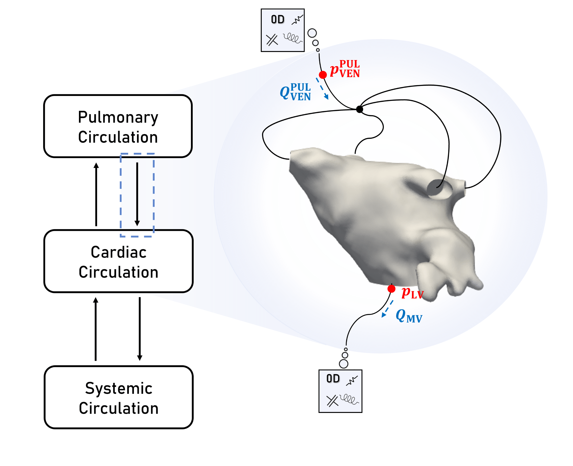
Figure 3: Relation between 0D variables and 3D domain in terms of boundary conditions that are prescribed to the 3D CFD problem. The coupling among the two models is enforced between the pulmonary and cardiac circulation. We highlight the left ventricular pressure $p_{\mathrm{LV}}$, mitral flux $Q_{\mathrm{MV}}$, pulmonary venous pressure $p_{\mathrm{VEN}}^{\mathrm{PUL}}$ and pulmonary venous flux $Q_{\mathrm{VEN}}^{\mathrm{PUL}}$.

We use the 0D model to calculate the fluid properties that serve as boundary conditions for the 3D fluid dynamics problem, as shown in Figure 3. The outlet pressure corresponds to the left ventricular pressure $p_{\mathrm{OUT}}=p_{\mathrm{LV}}$; the inlet pressure corresponds to the pulmonary venous pressure $p_{\mathrm{IN}}=p^{\mathrm{PUL}}_{\mathrm{VEN}}$. Concerning the Dirichlet inlet condition, we use the pulmonary veins flow rate $Q_{\mathrm{IN}}=Q^{\mathrm{PUL}}_{\mathrm{VEN}}$. We first carry out a fully 0D simulation, then, once the 0D solution becomes periodic, we use pressures and flowrates transient to set the boundary conditions to the 3D CFD problem. Our approach can be regarded as a geometric multiscale problem, solved via a splitting algorithm [61].

Moreover, the lumped-parameter model provides as output the volume of LA $V_{\mathrm{LA}}^{\mathrm{0D}}$, which is used to calibrate the displacement model, as we discuss in Section 2.2.3.

2.2.2 Accounting for AF in the lumped-parameter circulation model

The circulation model introduced in [42] is tuned to model a healthy individual; for this reason, we calibrate the parameters to simulate the AF pathology correctly. To the best of our knowledge, the only existing work in which a lumped-parameter model is used to simulate the AF pathology is [43]. The variations we use in this work are resumed in Figure 4. We underline that the ones applied to passive and active elastances of the right ventricle are introduced by us to fit the correct 3D volumes of real patients, while all the others are also employed in [43].

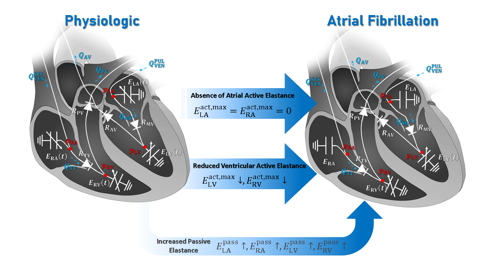
Figure 4: 0D lumped parameter Model changes to simulate an AF pathology. On the left, the original circulation model, on the right the model with null atrial active elastances.The two corrections (increased passive elastance and reduced $E_{\mathrm{RV}}^{\mathrm{act,max}}$) are necessary to fit the 3D patient-specific volumes. Variables names are coherent with model presented in [42].

To model the motion of the cardiac chambers, we use time-dependent elastances defined as [42]. Each elastance can vary in the following prescribed range:

$$E_{j}(t)\in[E_{j}^{\mathrm{pass}},E_{j}^{\mathrm{pass}}+E_{j}^{\mathrm{act,max}}],\qquad j\in\{\mathrm{RA},\mathrm{LA},\mathrm{RV},\mathrm{LV}\},$$

being $E_{j}^{\mathrm{pass}}$, $E_{j}^{\mathrm{act,max}}$ the passive and active elastances, respectively .

The effect of AF on the mechanical response of the cardiac tissue can be modelled by taking the active elastances equal to zero for both the atria, simulating hence the absence of the “atrial kick” [2, 4], i.e. $E_{\mathrm{LA}}^{\mathrm{act,max}}=E_{\mathrm{RA}}^{\mathrm{act,max}}=0$. In AF, this choice implies a constant value for the elastances of the two chambers, namely:

$$E_{\mathrm{LA}}(t)=E_{\mathrm{LA}}^{\mathrm{pass}},\qquad E_{\mathrm{RA}}(t)=E_{\mathrm{RA}}^{\mathrm{pass}}\qquad\forall t\in(0,T).$$

Under pathological transmission of the electric signal, we model the loss of ventricular contractility, reducing the active component of elastances in the ventricles.

To simulate the AF geometries, we increase the passive elastances of both atria and ventricles. This choice is fundamental to get the correct volumes and pulmonary venous pressure. Indeed, pulmonary hypertension has a connection with AF [62, 63], but without these corrections, the pressure values arising from the 0D model would become even higher than the pathological ones. After our calibration, the model also calculates lower values for left ventricular pressure $p_{\mathrm{LV}}$ than under physiological conditions, consistent with the pathological consequences of AF [64, 63]. The passive elastance correction is smaller in atria affected by the remodeling, which caused a volume increase. In fact, this consequence of the pathology is typically detected by AF lumped-parameter model [43].

2.2.3 Parametrization of the LA wall displacement

Following [60, 45, 46] we assume that the boundary datum $\boldsymbol{g}^{\mathrm{ALE}}$, introduced in Equation 1, can be expressed by means of the separation of variables as:

$$\boldsymbol{g}^{\mathrm{ALE}}(\boldsymbol{x},t)=\boldsymbol{F}^{\mathrm{ALE}}(\boldsymbol{x})\;h^{\mathrm{ALE}}(t)\qquad\mathrm{on}\;\partial\Omega_{t}\times(0,T).$$ (5)

In the following, we detail the construction of the two functions $h^{\mathrm{ALE}}$ and $\boldsymbol{F}^{\mathrm{ALE}}$. Let $V_{\mathrm{LA}}(t)$ be the LA volume; then, by using the Reynolds transport theorem (RTT) [65]:

$$\dfrac{\,\mathrm{d}V_{\mathrm{LA}}}{\mathrm{d}t}=\dfrac{\mathrm{d}}{\mathrm{d}t}\int_{\Omega_{t}}\mathrm{d}\boldsymbol{x}\overset{\mathrm{(RRT)}}{=}\int_{\partial\Omega_{t}}\boldsymbol{g}^{\mathrm{ALE}}\cdot\boldsymbol{n}\mathrm{d}\sigma=h^{\mathrm{ALE}}\int_{\partial\Omega_{t}}\boldsymbol{F}^{\mathrm{ALE}}\cdot\boldsymbol{n}\mathrm{d}\sigma,$$ (6)

we obtain the following definition of the time-dependent function:

$$h^{\mathrm{ALE}}(t)=\Bigg{(}\int_{\partial\Omega_{t}}\boldsymbol{F}^{\mathrm{ALE}}\cdot\boldsymbol{n}(t)d\sigma\Bigg{)}^{-1}\dfrac{\,\mathrm{d}V_{\mathrm{LA}}(t)}{\mathrm{d}t}.$$ (7)

Specifically, we set the LA volume to be equal to that computed via the 0D circulation model ($V_{\mathrm{LA}}(t)=V_{\mathrm{LA}}^{\mathrm{0D}}(t)$) for each time $t\in(0,T)$. This choice, together with the enforcement of boundary conditions provided from the circulation model, ensures that the compatibility of NS boundary conditions [44] is automatically satisfied by the mass conservation property of the 0D model [42].

2.2.4 Space-dependent function and LAA correction

The space-dependent component of the boundary function $\boldsymbol{F}^{\mathrm{ALE}}$ is constructed by considering two different components on the corresponding reference domain:

$$\widehat{\boldsymbol{F}}^{\mathrm{ALE}}(\widehat{\boldsymbol{x}})=\widehat{\boldsymbol{f}}^{\mathrm{ALE}}(\widehat{\boldsymbol{x}})+\widehat{\boldsymbol{f}}_{\mathrm{LAA}}^{\mathrm{ALE}}(\widehat{\boldsymbol{x}}).$$ (8)

In Equation 8, we separate the motion of the whole chamber, modelled by $\widehat{\boldsymbol{f}}^{\mathrm{ALE}}$, from the one of the LAA, which is separately described by $\widehat{\boldsymbol{f}}_{\mathrm{LAA}}^{\mathrm{ALE}}$. A correct calibration of these two functions generates a displacement that can be adapted to the LAA morphology. Moreover, by introducing this distinction, we have control on the LAAEF, which can be set to be coherent with the clinical measurements found in literature concerning the pathologic situation of the patient, providing hence a better estimate of the blood motion inside the most dangerous region in terms of thrombous formation [66, 67, 68].

We define the global component $\widehat{\boldsymbol{f}}^{\mathrm{ALE}}$ as:

$$\widehat{\boldsymbol{f}}^{\mathrm{ALE}}(\widehat{\boldsymbol{x}})=\widehat{\psi}(\widehat{\boldsymbol{x}})\;\left(\widehat{\boldsymbol{x}}-\widehat{\boldsymbol{x}}_{\mathrm{G}}\right),$$ (9)

where the second term is a vector field directed to the centre of mass of the atrium $\widehat{\boldsymbol{x}}_{\mathrm{G}}$. We compute the function $\widehat{\psi}$ as a normalised product:

$$\widehat{\psi}(\widehat{\boldsymbol{x}})=\dfrac{\widehat{\varphi}(\widehat{\boldsymbol{x}})\;\left(1-\widehat{\varphi}(\widehat{\boldsymbol{x}})\right)}{\underset{\widehat{\boldsymbol{x}}\in\partial\widehat{\Omega}}{\max}\left\{\widehat{\varphi}(\widehat{\boldsymbol{x}})\;\left(1-\widehat{\varphi}(\widehat{\boldsymbol{x}})\right)\right\}},$$ (10)

being $\widehat{\varphi}$ solution of the following Laplace-Beltrami problem [69]:

$$\begin{cases}-\Delta_{\Gamma}\widehat{\varphi}=0&\mathrm{in}\;\partial\widehat{\Omega},\\ \widehat{\varphi}=0&\mathrm{on}\;\bigcup_{j=1}^{4}\widehat{\Gamma}^{\mathrm{PV}_{j}},\\ \widehat{\varphi}=1&\mathrm{on}\;\widehat{\Gamma}^{\mathrm{MV}}.\end{cases}$$ (11)

By defining $\widehat{\psi}:\partial\widehat{\Omega}\to[0,1]$ as described, we get a smooth function which is zero on the inlet and outlet sections of our computational domain, and non-null in the main chamber, as displayed in Figure 5.

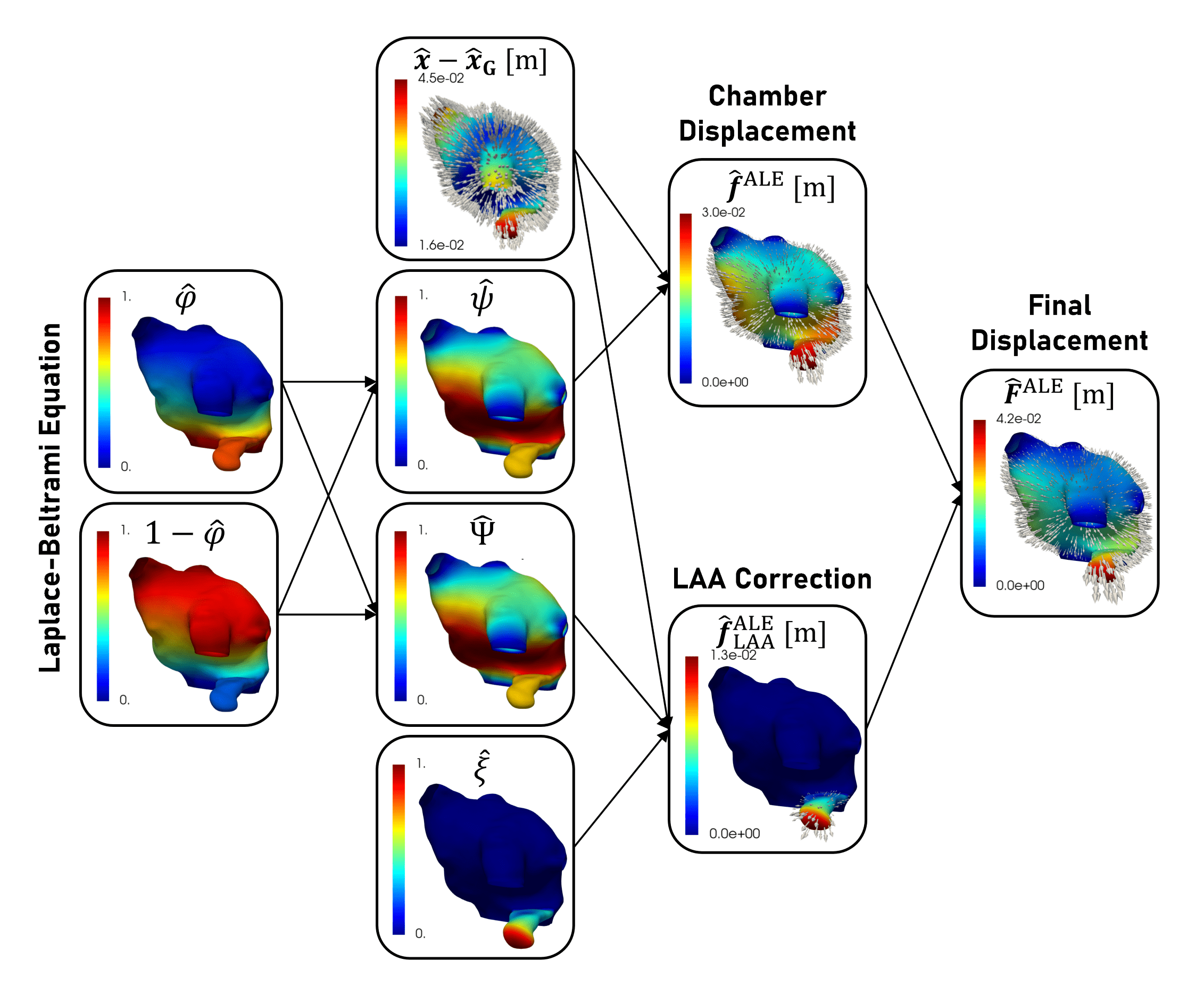
Figure 5: Complete procedure to derive the spatial component of the boundary displacement $\boldsymbol{F}^{\mathrm{ALE}}$. We start from the Laplace-Beltrami solution $\widehat{\varphi}$, the LAA smoothing function $\widehat{\xi}$ and the distance from centre of mass $\widehat{\boldsymbol{x}}-\widehat{\boldsymbol{x}}_{\mathrm{G}}$. The image shows also the partial results needed: $\widehat{\psi}$, $\widehat{\Psi}$, $\boldsymbol{f}^{\mathrm{ALE}}$,$\boldsymbol{f}_{\mathrm{LAA}}^{\mathrm{ALE}}$

.

Analogously, we construct the function $\widehat{\boldsymbol{f}}_{\mathrm{LAA}}^{\mathrm{ALE}}$ as follows:

$$\widehat{\boldsymbol{f}}_{\mathrm{LAA}}^{\mathrm{ALE}}(\widehat{\boldsymbol{x}})=\widehat{\Psi}(\widehat{\boldsymbol{x}})\;\widehat{\xi}(\widehat{\boldsymbol{x}})\;(\widehat{\boldsymbol{x}}-\widehat{\boldsymbol{x}}_{\mathrm{G}}^{\mathrm{LAA}}),$$ (12)

where $\widehat{\boldsymbol{x}}_{\mathrm{G}}^{\mathrm{LAA}}$ is the center of mass of the LAA and we define it as $\widehat{\Psi}(\widehat{\boldsymbol{x}})=k\;\widehat{\psi}(\widehat{\boldsymbol{x}})$. The use of a multiplicative constant $k$ allows us to vary the magnitude of the LAA contraction, according to the LAAEF, which characterizes the pathological situation of the patient. By defining $\widehat{\boldsymbol{f}}_{\mathrm{LAA}}^{\mathrm{ALE}}$ as explained, we get a displacement which is directed towards the center of mass of the LAA; moreover, it is fundamental the use of a function $\widehat{\xi}$ to localize the support only at the LAA surface, indeed the changes need to be located only in this region.

2.3 Setup of numerical simulations

We carry out numerical simulations on four ideal patients. In particular, we considered a LA geometry related to a subject with physiological conditions, assuming first sinus rhythm and then AF, and two geometries of patients really affected by AF. The imaging method used to reconstruct medical images is the diffusion tensor magnetic resonance imaging, which allows better resolution of the thin atrial wall [41]. The hearts were of donors from National Disease Research Interchange (Philadelphia, PA). Geometric and clinical information for the three patients are resumed in Table 1. The volumes of patients AF2 and AF3 are larger than those normally detected under physiological conditions. These values suggest an atrial remodeling caused by the AF pathology; hinting at the possibility of a persistent AF.

Geometry	P1	P2	P3
Age	$55$ Years	$86$ Years	$94$ Years
Gender	Male	Male	Female
Pathology	None	AF	AF
LA Max Volume [$\mathrm{cm}^{3}$]	$58.06$	$85.55$	$69.39$
RA Max Volume [$\mathrm{cm}^{3}$]	$69.39$	$55.76$	$36.33$
ID in repository [40]	$7$	$6$	$5$

Table 1: Information of the geometries detected from images.

2.3.1 Meshes

As we can see in Figure 6, we build a hexahedral mesh with a heterogeneous size $h_{K}$. We perform a refinement in the LAA to capture the geometrical features of this region and near the MV to correctly represent the valve using the RIIS method. We use a value of $\varepsilon=1.3\;\mathrm{mm}$ due to medical estimates of $2.6\;\mathrm{mm}$ of the thickness of the MV leaflet [70, 71] ($\varepsilon$ represents the half-thickness of the valve leaflets). Concerning opening $\Delta\tau_{\mathrm{O}}$ and closure $\Delta\tau_{\mathrm{C}}$ duration of the MV, we consider literature estimates, and we set $\Delta\tau_{\mathrm{O}}=20\;\mathrm{ms}$ [72] and $\Delta\tau_{\mathrm{C}}=60\;\mathrm{ms}$ [73]. We consider the opening of the valve when the pressure of a control volume inside the LA is higher than the one computed inside a volume downwind the valve. The valve closure starts at a fixed time, imposed when $\dot{V}_{\mathrm{LV}}$ of the 0D model simulation becomes negative, i.e. when a condition of reversed flow is detected on the outlet section [74].

The MV geometries were not available in the repository [39, 40]. For this reason, we adapt the valve geometry provided by Zygote [75] to the orifice of the patient-specific LA. Moreover, the leaflet displacement we prescribe is the same that has been designed in [60].

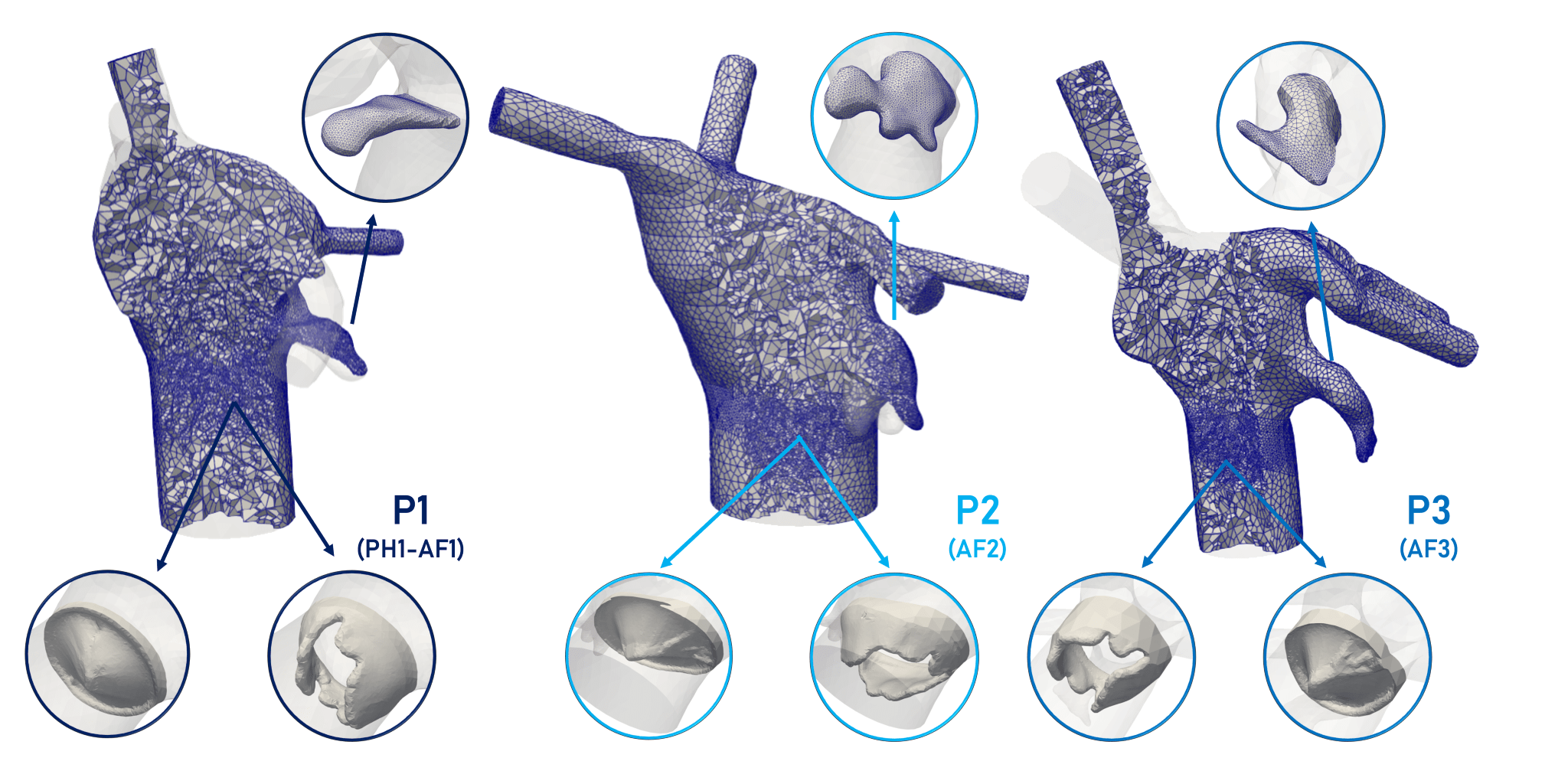
Figure 6: Hexaedral meshes used to simulate the patients haemodynamics, with the detail of: LAA morphology, the MV in open and closed configurations. Meshes are refined in the LAA region, to correctly capture the geometrical features, and near the MV, in order to represent its leaflet by means of the RIIS method.

Concerning the pulmonary veins, we add some rigid tubes to the domain to obtain at the LA inlet a fully developed flow and to reduce the influence of the parabolic profile choice.

Using the VMTK library [76], we first generate a tetrahedral mesh, then we use mesh tethex [77] to obtain a hexaedral mesh in which each tetrahedron is split into four hexahedra preserving the aspect ratio of the original element. Information about the constructed meshes is reported in Table 2. A more detailed description of the preprocessing of tools we used to generate the meshes can be found in [78].

Mesh	P1	P2	P3
(Patient)	(PH1-AF1)	(AF2)	(AF3)
Number of Cells	$120\,860$	$182\,540$	$110\,472$
Velocity $\mathrm{DOFs}$	$411\,873$	$614\,631$	$378\,879$
Pressure $\mathrm{DOFs}$	$137\,291$	$204\,877$	$126\,293$
Total $\mathrm{DOFs}$	$549\,164$	$819\,508$	$505\,172$
$h_{K}^{\mathrm{max}}\;[\mathrm{mm}]$	$5.95$	$5.44$	$6.15$
$h_{K}^{\mathrm{min}}\;[\mathrm{mm}]$	$0.43$	$0.40$	$0.38$
$h_{K}^{\mathrm{avg}}\;[\mathrm{mm}]$	$1.76$	$1.69$	$1.82$

Table 2: Details of the hexaedral meshes generated to carry out CFD simulations. The DOFs are referred to linear finite elements for velocity and pressure.

2.3.2 CFD simulations

All the simulations, based on the mathematical models we have shown, have been executed in $\texttt{life}^{\texttt{x}}$ [79, 80], a high-performance C++ FE library developed within the iHEART project, mainly focused on cardiac simulations and based on deal.II finite element core [81]. Numerical simulations are carried out on the cluster of the Department of Mathematics, Politecnico di Milano. Specifically, the simulations PH1, AF1, and AF2 were run in the Gigat queue (6 nodes, 12 Intel Xeon E5-2640v4 @ 2.40GHz, 120 cores, 384GB RAM, O.S. Centos 6.7) using 2 nodes with 20 cores each, and AF3 was run in the Gigatlong cluster (5 nodes, 10 Intel Xeon Gold 6238 @ 2.10GHz, 280 cores, 2.5TB RAM) using 1 node with 56 cores.

Blood density and dynamic viscosity are set equal to $\rho=1.06\cdot 10^{3}\;\mathrm{kg/m^{3}}$ and $\mu=3.5\cdot 10^{-3}\;\mathrm{kg/(m\cdot s)}$, respectively. We simulate six heartbeats, of period $T_{\mathrm{HB}}=1\,\mathrm{s}$, starting from a null initial condition. However, to filter out the unphysical consequences of this choice, we discard the first two heartbeats and we consider the phase-averaged velocity, defined over $N_{\mathrm{HB}}$ heartbeats, as:

$$\langle\boldsymbol{u}(\boldsymbol{x},t)\rangle=\dfrac{1}{N_{\mathrm{HB}}}\sum_{n=1}^{N_{\mathrm{HB}}}\boldsymbol{u}(\boldsymbol{x},t+(n-1)T_{\mathrm{HB}}).$$ (13)

2.3.3 Lagrangian simulations

The use of Lagrangian simulations to detect indicators can provide additional information on the haemodynamics [17, 53]. We perform numerical simulations of the movement of red blood cells inside the LA, using as velocity field the result of the NS simulations. In addition, we consider the introduction of $N_{H}$ parcels in each heartbeat. In particular, we consider the injection of a volume of blood $V_{\mathrm{Inj}}=\int_{0}^{T_{\mathrm{HB}}}Q_{\mathrm{VEN}}^{\mathrm{PUL}}(t)\mathrm{d}t$.

We use the injected volume to estimate the number $N_{P}$ of cells entering the atrium during a single heartbeat, also considering that the number of red blood cells in a cubic millimetre is approximately $5$ millions [83]. Our simulation is designed to obtain a constant approximate weight $\omega=N_{P}/N_{H}\simeq 1409$, common to all cases, where $N_{P}$ is the number of simulated red blood cells.

The number of parcels injected at any timestep can be computed as follows: $n_{H}(t)=\dfrac{Q_{\mathrm{VEN}}^{\mathrm{PUL}}(t)}{V_{\mathrm{Inj}}}\,\Delta\tau\,N_{\mathrm{H}},$ where $\Delta\tau$ is the time step we choose for the Lagrangian simulation. We split the injection among the four pulmonary veins according to the flow repartition factor introduced in Equation 3; the parcels are distributed in a hemisphere centered at the beginning of the pulmonary vein extension and with the same radius of the cylinder. The initial position of the parcels is randomly chosen within the hemisphere, and an example can be seen in Figure 7.

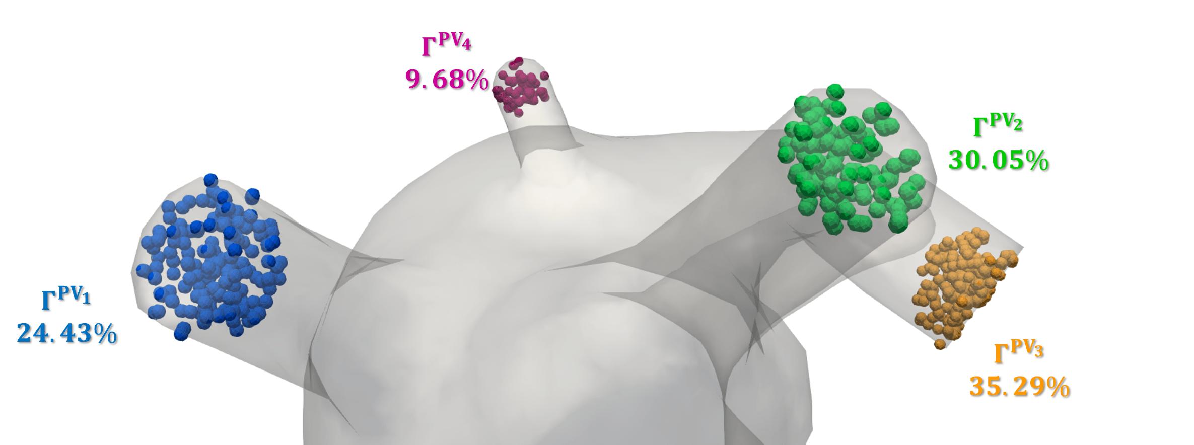
Figure 7: Position of parcels injection in cases PH1 and AF1 associated to the inlet sections $\Gamma^{PV}_{j}$ and to the flow rate $\zeta_{j}$ in Equation 3.

More information on the equation of motion of the parcels and the construction of Eulerian fields from the Lagrangian perspective can be found in the supplementary material and in [78]. This type of modelling is a first attempt to detect the indicators to estimate thrombotic risk. As we are aware of the limitations of this indicator, we plan to further investigate it in the future. For example, we can improve the equations of motion (i.e. introducing wall attachment properties as in [84]).

3 Results

In this Section, we show the results of numerical simulations. Specifically, we present the results of the circulation model in Section 3.1 and the 3D Eulerian and Lagrangian indicators in Sections 3.2 and 3.3, respectively. Section 3.4 is devoted to the introduction of the new hemodynamic indicator.

3.1 Results of lumped-parameter model

The parameter values used in the simulation of the lumped-parameter model have to be calibrated starting from values present in the literature [85, 42, 86, 43]. However, due to the requirement to fit the information from the medical images and the pathological situation, they need to be separately tuned for each patient. We report the parameters that we keep common to all cases in Table 7(a). Instead, in Table 7(b), we store the chamber elastances in the four simulated cases. We choose the elastances starting from literature values in [42], and they are manually calibrated to fit the volume of the atrial chambers and to reach reasonable ejection fractions.

In Table 3, we list the Left Atrial Ejection Fraction (LAEF) and LAAEF, calculated after our procedure and defined as:

$$\mathrm{LAEF}=\dfrac{V_{\mathrm{LA}}^{\mathrm{max}}-V_{\mathrm{LA}}^{\mathrm{min}}}{V_{\mathrm{LA}}^{\mathrm{max}}},\quad\mathrm{and}\quad\mathrm{LAAEF}=\dfrac{V_{\mathrm{LAA}}^{\mathrm{max}}-V_{\mathrm{LAA}}^{\mathrm{min}}}{V_{\mathrm{LAA}}^{\mathrm{max}}},$$ (14)

respectively. We remark that the maximum volumes are directly retrieved by medical images; whereas the minimum ones are determined after the application of the displacement. The in-silico values we compute are in accordance with the clinical measurements, for both LAEF [87, 88], and LAAEF [47], making the whole displacement procedure significant and reliable.

Patient	Pathology	Indicator	Simulated	Clinical	Reference
(Geometry)			value	measurement
PH1 (P1)	None	LAEF (%) LAAEF (%)	$50.49$ $77.81$	$45.1\div 64.1$ $62.5\div 86.5$	[87] [47]
AF1 (P1)	Paroxysmal AF	LAEF (%) LAAEF (%)	$30.72$ $62.72$	$10.0\div 50.0$ $50.0\div 69.0$	[88] [47]
AF2 (P2)	Persistent AF	LAEF (%) LAAEF (%)	$18.48$ $38.94$	$6.0\div 26.0$ $32.4\div 63.2$	[88] [47]
AF3 (P3)	Persistent AF	LAEF (%) LAAEF (%)	$21.17$ $53.45$	$6.0\div 26.0$ $32.4\div 63.2$	[88] [47]

Table 3: Patient information from images and modelling assumptions with simulated values of atrial and auricle ejection fractions, clinical measurement are intended in a range (min $\div$ max).

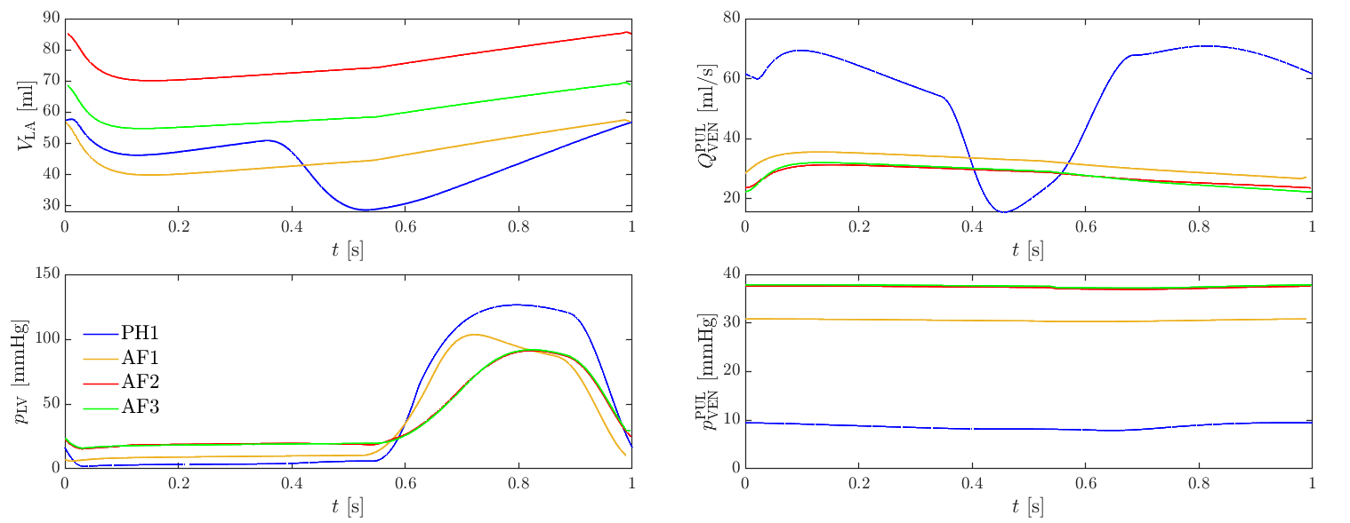
Figure 8: Results of the lumped-parameter model simulations for the four patients: left atrial volume $V_{\mathrm{LA}}$ (top, left), pulmonary venous flux $Q_{\mathrm{VEN}}^{\mathrm{PUL}}$ (top, right), left ventricular pressure $p_{\mathrm{LV}}$ (down, left) and pulmonary venous pressure $p_{\mathrm{VEN}}^{\mathrm{PUL}}$ (down, right). These transients are then used as boundary data for the 3D CFD simulations.

We report the volume of LA, the pulmonary venous flow rate and pressure, and the ventricular pressure in Figure 8, for the four simulated cases. We recall that these functions are taken as output from the 0D model and used as boundary data for our 3D CFD simulation.

3.2 CFD Eulerian indicators

We report the velocity magnitude in Figure 9 in a single heartbeat. The velocity magnitude is larger in physiologic conditions than in AF ones during the whole heartbeat. This behaviour is evident during the E-wave ($t\simeq 0.10\,\mathrm{s}$), whereas the A-wave is present only in the patient PH1 ($t=0.40\,\mathrm{s}$). When the MV is closed, we can notice the difference in contraction of the two atrial chambers, due to the contractile reduction in fibrillation ($t\simeq 0.60\,\mathrm{s}$).

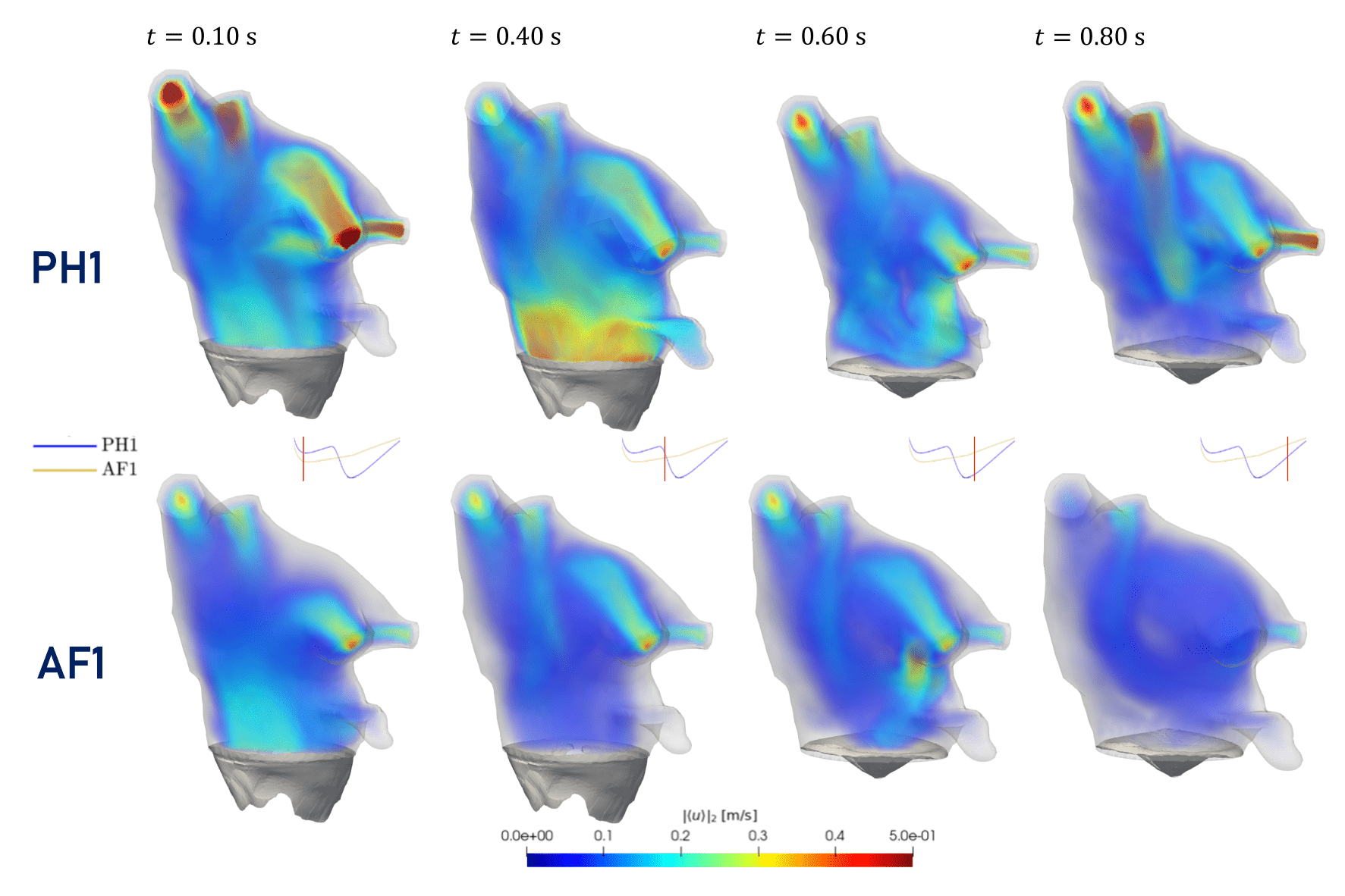
Figure 9: Volume rendering of phase-averaged velocity magnitude $|\langle\boldsymbol{u}\rangle|_{2}$ at different time instants in physiologic and AF conditions considering the same atrial geometry. The time instants are reported on the volume transients to distinguish diastolic and systolic phases.

Patient	Indicator	In silico	Clinical	Reference
		result	measurement
PH1	Peak velocity veins [m/s] Peak velocity [m/s] Mean velocity [m/s] E-peak velocity [m/s] A-peak velocity [m/s] E/A ratio [-] Peak LAA emptying velocity [m/s]	$0.474$ $0.775$ $0.149$ $0.918$ $0.544$ $1.680$ $0.428$	$0.370\div 0.600$ $0.560\div 1.060$ $0.130\div 0.170$ $0.740\div 1.040$ $0.520\div 1.040$ $0.800\div 1.870$ $0.279\div 0.432$	[89] [89] [10] [90] [90] [91, 90] [92]
AF1	Peak velocity veins [m/s] Peak velocity [m/s] Mean velocity [m/s] E-peak velocity [m/s] Peak LAA emptying velocity [m/s]	$0.276$ $0.480$ $0.096$ $0.612$ $0.413$	$0.250\div 0.540$ $0.470\div 0.970$ $0.080\div 0.140$ $0.443\div 0.771$ $0.208\div 0.428$	[89] [89] [10] [93] [92]
AF2	Peak velocity veins [m/s] Peak velocity [m/s] Mean velocity [m/s] E-peak velocity [m/s] Peak LAA emptying velocity [m/s]	$0.288$ $0.177$ $0.058$ $0.664$ $0.366$	- $0.150\div 0.290$ $0.056\div 0.160$ $0.516\div 0.812$ $0.160\div 0.390$	- [92] [92] [93] [92]
AF3	Peak velocity veins [m/s] Peak velocity [m/s] Mean velocity [m/s] E-peak velocity [m/s] Peak LAA emptying velocity [m/s]	$0.149$ $0.217$ $0.065$ $0.591$ $0.347$	- $0.150\div 0.290$ $0.056\div 0.160$ $0.516\div 0.812$ $0.160\div 0.390$	- [92] [92] [93] [92]

Table 4: Comparison between in silico results and literature data for the four patients in terms of the following biomarkers: velocity magnitudes in LA, at the entrance of the pulmonary veins, at the mitral orifice and at the LAA ostium.

In Table 4, we report a validation comparing the peak and mean velocities within the entire LA with medical estimates from MRI images in [89, 10]. In addition, we report the LAA emptying peak velocity, which is a widely used indicator because it correlates with thrombus formation.

We report the velocities computed at the MV section in Figure 10 and we compare our results with the literature estimates from Doppler imaging [93, 90, 91]. The value is computed by space-averaging the velocity values inside a spherical volume between the leaflet of MV, coherently with the procedure used starting from Doppler images. The case PH1 also allows to perform a validation with the A-wave, not present in AF, peak velocity and then with the E/A ratio, which is an important medical parameter [91, 90]. Finally, we report the mean velocities between the four pulmonary veins computed at the LA entrance in Figure 10.

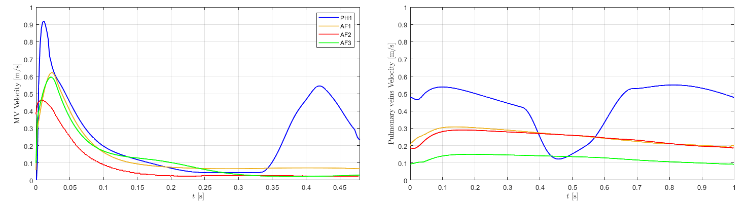
Figure 10: MV transmitral velocity profiles (left) and pulmonary veins velocity profiles (right) in the four patients.

Flow stasis

The flow stasis is an indicator representing the fraction of time of the heartbeat in which the velocity magnitude in a specific point is smaller than $0.1\;\mathrm{m/s}$ [92]. This threshold value is consistent with the sensitivity analysis performed in [11]. From this indication, we define it as follows:

$$\mathrm{F_{S}}(\boldsymbol{\hat{x}})=\dfrac{1}{T_{\mathrm{HB}}}\int_{0}^{T_{\mathrm{HB}}}\chi_{\{|\langle\boldsymbol{u}\rangle(\boldsymbol{\hat{x}},t)|_{2}<0.1\mathrm{m/s}\}}(\boldsymbol{\hat{x}},t)\mathrm{d}t\qquad\mathrm{in}\;\widehat{\Omega},$$ (15)

where $\chi$ is a characteristic function. An accurate estimate of flow stasis is fundamental to determine thromboembolic risk, coherently with the Virchow’s triad [7]. The volume rendering of the flow stasis for the four patients can be observed in Figure 11.

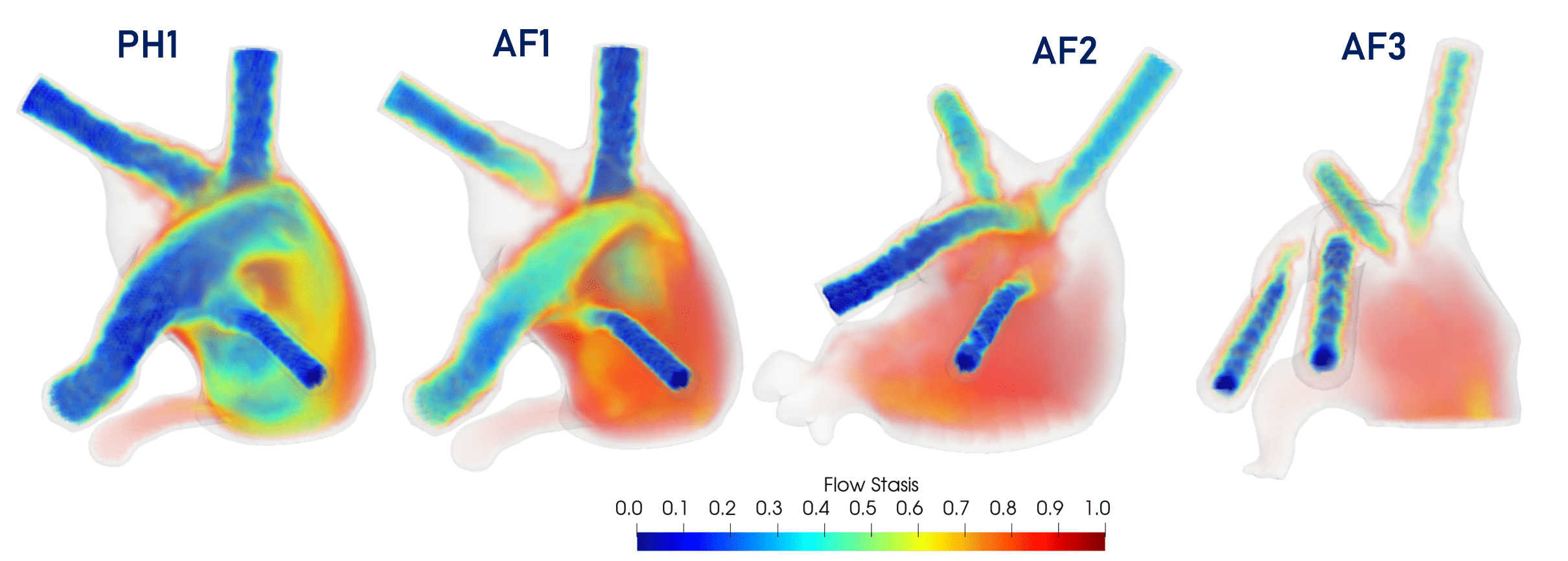
Figure 11: Volume rendering of the flow stasis indicator $\boldsymbol{\mathrm{F}_{\mathrm{S}}}$ in the atrial chamber, for all the four cases.

However, because of the lower quality of the imaging compared to the CFD resolution it is not possible to make a detailed comparison with the magnitude of the clinical measurements. For this reason, we calculate a spatial-averaged value of flow stasis as in [11]. The average is computed neglecting from the atrial domain a boundary layer of $3\;\mathrm{mm}$ width. We report the final values in Table 5.

Patient	In silico	Clinical	Reference
	result	measurement
PH1	$0.333$	$0.128\div 0.502$	[11, 92]
AF1	$0.806$	$0.222\div 0.896$	[11, 92]
AF2	$0.853$	$0.222\div 0.896$	[11, 92]
AF3	$0.873$	$0.222\div 0.896$	[11, 92]

Table 5: Comparison between in silico results and data coming from literature for the four patients in terms of space-averaged flow stasis.

Time-averaged wall shear stress

The shear stress at the wall is related to endothelial shear, formation of new tissues and plaques, and promoting of neointimal hyperplasia [94]. Specifically, we consider the time-averaged wall shear stress (TAWSS) defined as [23]:

$$\mathrm{TAWSS}(\langle\boldsymbol{u}\rangle)=\dfrac{1}{T_{\mathrm{HB}}}\int_{0}^{T_{\mathrm{HB}}}|\boldsymbol{\tau}_{W}(\langle\boldsymbol{u}\rangle)|_{2}\,\mathrm{d}t\qquad\mathrm{on}\;\partial\widehat{\Omega},$$ (16)

where $\boldsymbol{\tau}_{W}(\langle\boldsymbol{u}\rangle)$ is the wall shear stress (WSS). In Figure 12, we report the TAWSS for all patients.

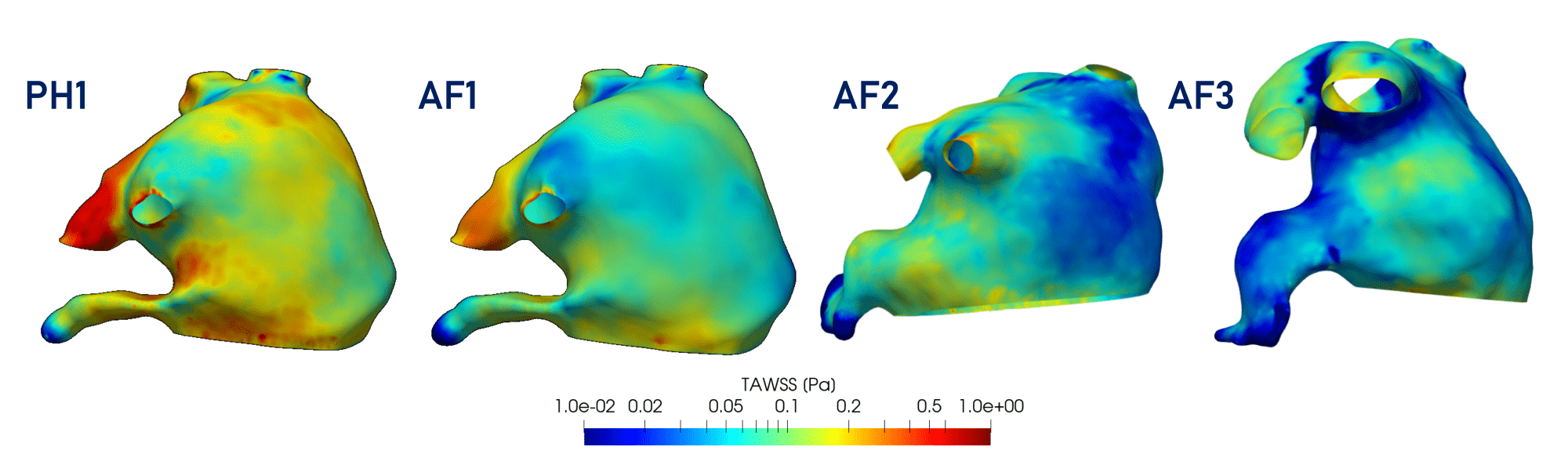
Figure 12: TAWSS indicator computed on the endocardial surface of atrial chamber for all the four patients.

Endothelial Cell Activation Potential

Another commonly used indicator to detect the endothelial susceptibility and the thrombus formation probability is the Endothelial Cell Activation Potential (ECAP) indicator [95], defined as:

$$\mathrm{ECAP}(\langle\widehat{\boldsymbol{u}}\rangle)=\dfrac{\mathrm{OSI}(\langle\widehat{\boldsymbol{u}}\rangle)}{\mathrm{TAWSS}(\langle\widehat{\boldsymbol{u}}\rangle)},$$ (17)

OSI being the oscillatory shear index [94]. OSI is high in regions where WSS changes much during the heart cycle. Thus, ECAP detects high oscillatory and low shear stress regions. In Figure 13, we report the ECAP values focus on the LAA wall.

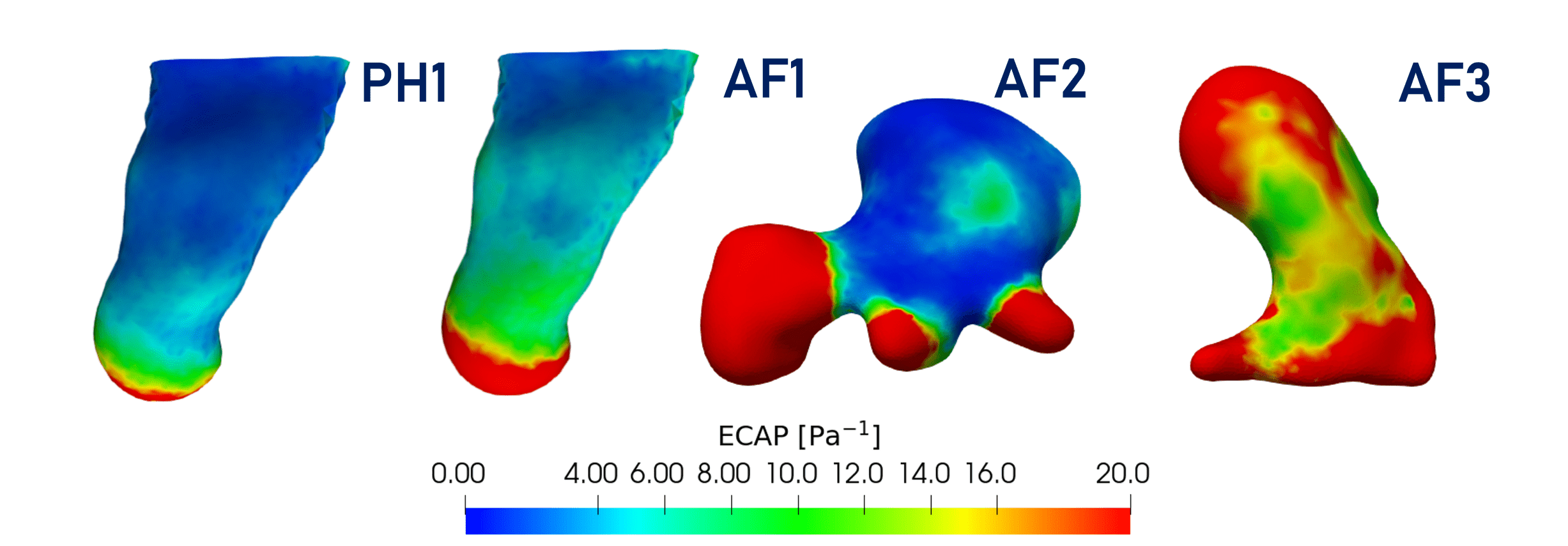
Figure 13: ECAP indicator computed on the endocardial surface for all the four patients. For each patient, the visualization is restricted only to the LAA.

3.3 CFD Lagrangian indicators

In the following, we analyze the Lagrangian indicators with the simulations carry out as explained in Section 2.3.3.

Mean age of blood

We consider the injection of particles during all simulated cardiac cycles to construct some Lagrangian fields from the Lagrangian perspective, with the information of all simulated heartbeats. The computation of results based on the age of the blood gives us a new perspective to analyse the regions in which the particles remain for a long time in the atrium, increasing the thrombosis. Additional details on the definition of this field can be found in the Supplementary Material.

The mean age field of red blood cells detects regions in which the blood particles stagnate in the atrium. This indicator was proposed by [19] to analyse the age of the blood in LA subjected to AF. We denote by $m_{1}$ and its definition is provided in the Supplementary Material. In Figure 14, we can observe the $m_{1}$ field for the four simulated cases.

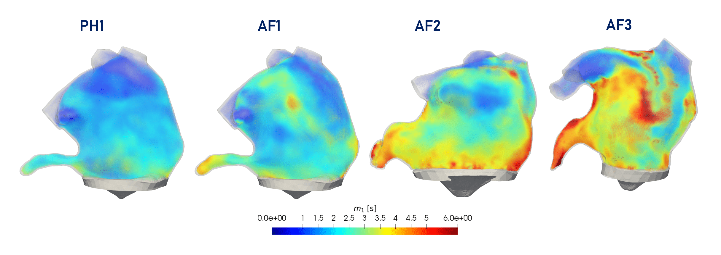
Figure 14: Volume rendering of the blood mean age field $m_{1}$ (in seconds) in the atrial chamber for all the four patients.

Washout of blood

We compute the washout field $\psi_{\bar{t}}$ at the final time, as defined in the supplementary material. In particular, in the simulation we choose $\bar{t}=2\,\mathrm{s}$, we consider a contribution to the field equal to 1 from the particles injected in the first two cycles and equal to 0 for the others. The resulting field gives values between 0 and 1, where:

• $\psi_{\bar{t}}\gtrsim 0$, means that there is a local prevalence of particles injected after $\bar{t}$;

• $\psi_{\bar{t}}\lesssim 1$, means that there is a local prevalence of particles injected before $\bar{t}$.

In Figure 15, we show the washout field at time $t=6\,\mathrm{s}$ using some slices in the LA volume and in its appendage.

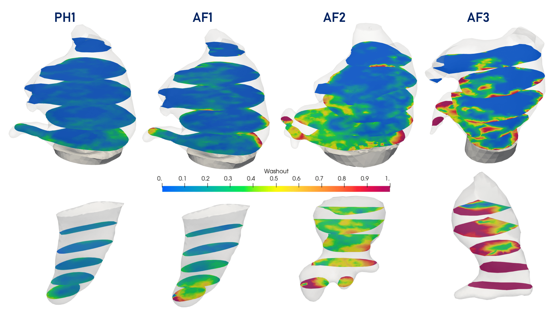
Figure 15: Washout field $\psi_{2}$ represented over some slices both in the atrial chambers (first row) and in the LAA (second row) for all the four patients at time $t=6\,\mathrm{s}$.

Residence time and total path length

In this section, we consider particle injection during the first heartbeat only. We analyse the distributions of some Lagrangian indicators in the following five heartbeats of simulation. A video of the motion of the parcels used in this section is provided as supplementary material. In particular, we consider the distribution of two quantities: the Total Path Length (TPL) is the length travelled by a parcel before leaving the LA; the Residence Time (RT) is the time spent by a particle inside the LA. We report the indicators distributions and a scatter plot correlating RT and TPL in Figure 16.

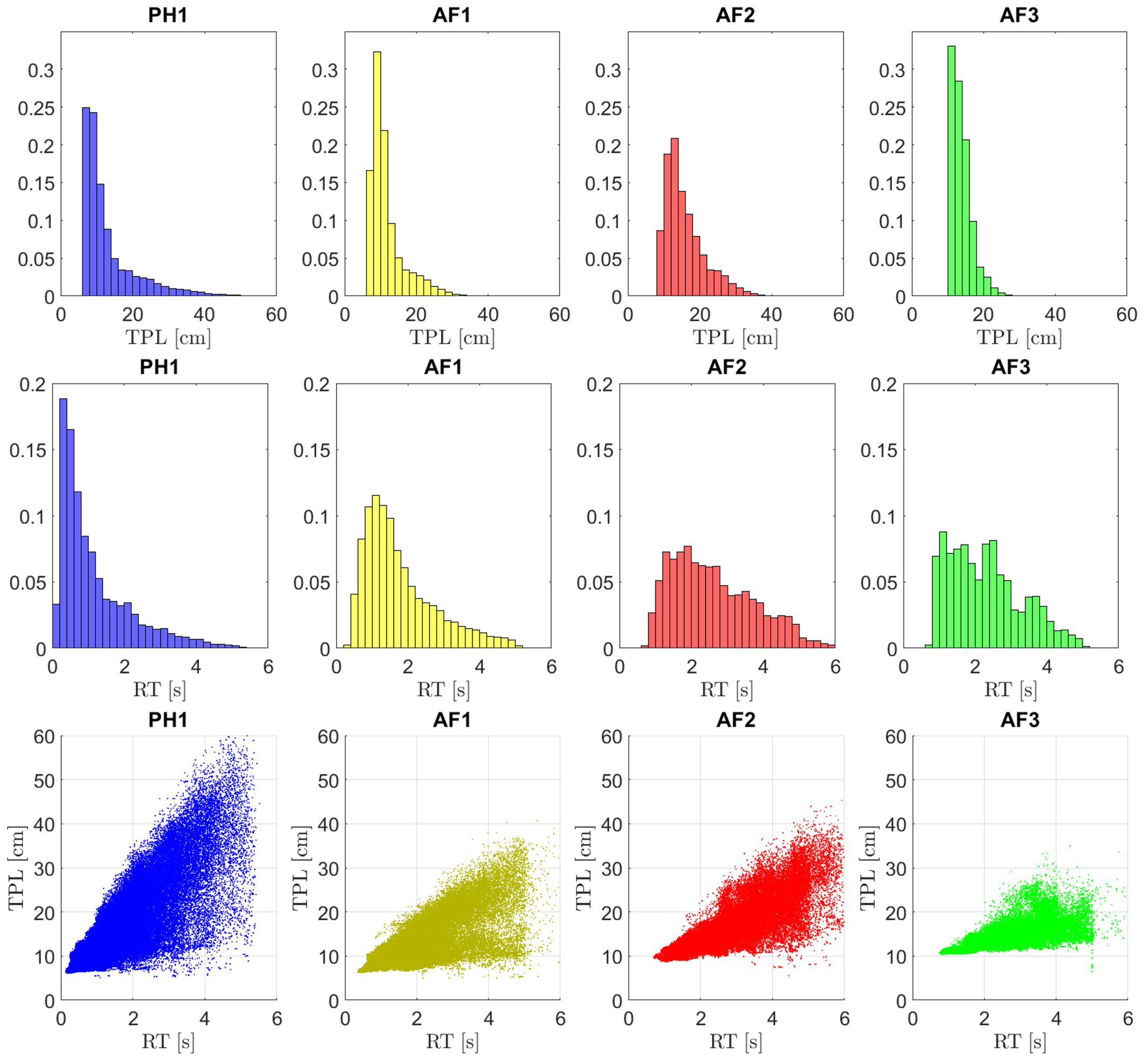
Figure 16: TPL histogram distribution (first row), RT histogram distribution (second row) and correlation scatter plot (third row) for all the four patients.

3.4 Age Stasis: a new haemodynamic indicator

In order to summarise the high complexity of blood flow within LA, we introduce a novel haemodynamic indicator, which we call Age Stasis (AS), by combining results from both Eulerian and Lagrangian analyses of haemodynamics in LA. Our goal is to construct an indicator which considers, at the same time, information about the stagnation of the flow and the oldness of the blood cells. We define AS as:

$$\mathrm{A_{S}}(\boldsymbol{x})=\mathrm{F_{S}}(\boldsymbol{x})\dfrac{m_{1}(\boldsymbol{x})}{T}.$$ (18)

In this way, we are constructing an indicator which accounts for the flow stasis $\mathrm{F_{S}}(\boldsymbol{x})$, that localizes regions in which the blood flows slowly, and a relative mean age of the blood $m_{1}(\boldsymbol{x})/T$, being $T$ the final time of the simulation. Thus, we can distinguish regions in which the flow is slow and the particles present are old $(\mathrm{A_{S}}\simeq 1)$. In order to detect dangerous regions, we neglect $(\mathrm{A_{S}}\simeq 0)$ the ones in which:

• the flow is slow $(\mathrm{F_{S}}\simeq 1)$, but the particles are not old $(m_{1}\ll T)$; therefore, there are no particles stationing at that point for a long time. In particular, the boundary layers, where flow stasis is high, are not always associated with a high thrombosis risk;

• the flow is fast $(\mathrm{F_{S}}\simeq 0)$, but the particles are old $(m_{1}\simeq T)$. These regions are the ones that require more time to be reached by particles because of their location, but are not stationing points. These regions are not at risk of thrombi formation, because of the absence of the stasis factor. The mitral orifice is the best example of this scenario.

The result is a useful dimensionless indicator which assumes values between 0 and 1. We observe in Figure 17A the indicator computed in the four simulated cases.

In order to provide a more synthetic quantification of the thrombogenic risk, we introduce the Age Stasis Volume function as:

$$V_{\mathrm{AS}}(\theta)=\int_{\widehat{\Omega}}\chi_{\{\mathrm{A_{S}}(\boldsymbol{x})\geq\theta\}}\mathrm{d}\boldsymbol{x},$$ (19)

This function, given a value $\theta$ of AS, returns the volume $V_{\mathrm{AS}}(\theta)$ of blood within the LA characterised by a value of AS greater than $\theta$. Thus, $V_{\mathrm{AS}}(\theta)$ is useful for investigating the percentage of LA volume associated with a high thrombogenic risk. A comparison between the Age Stasis Volume functions computed in the four simulated cases is provided in Figure 17B. By choosing specific values of $\mathrm{A_{S}}$ we obtain the results in Table 6. Finally, in Figure 17C, we show the distribution of AS values in the LA volume, constructed using a random sampling of the domain.

Parameter	PH1	AF1	AF2	AF3
$\Big{(}V_{\mathrm{LA}}-V_{\mathrm{AS}}(0.1)\Big{)}/V_{\mathrm{LA}}$	$41.3\%$	$11.7\%$	$5.70\%$	$4.20\%$
$V_{\mathrm{AS}}(0.5)/V_{\mathrm{LA}}$	$0.7\%$	$5.5\%$	$23.3\%$	$27.5\%$

Table 6: Age Stasis Volumes (%) significant values.

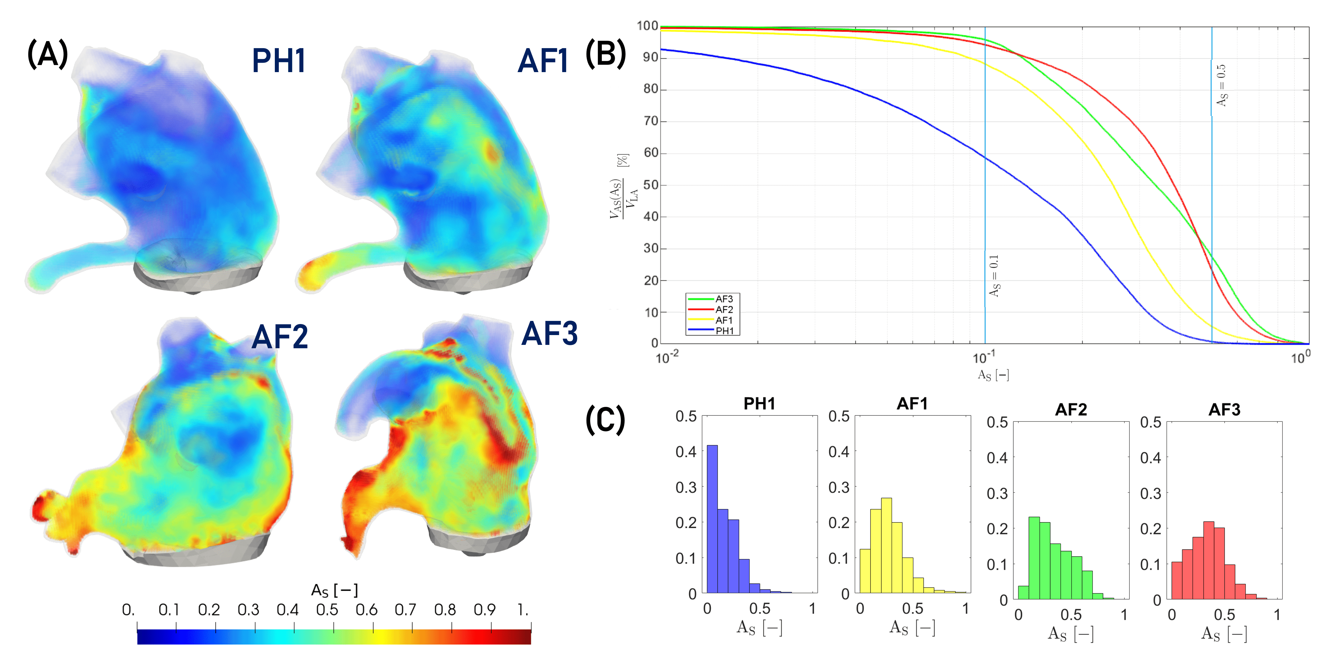
Figure 17: Volume rendering of Age Stasis inside the LA (A), Age Stasis Volume function plotted against the Age Stasis values ($x$-axis in logaritmic scale) (B) and histograms of the Age Stasis distributions functions in the LA (C). All the indicators are reported for all the four patients.

4 Discussion

In the following, we discuss the numerical results we obtain. Particularly, we analyze the results of the lumped parameter model in Section 4.1. The discussion of the Eulerian and Lagrangian indicators is provided in Sections 4.2 and 4.3, respectively. Finally Section 4.4 is devoted to the discussion of the new hemodynamic indicator.

4.1 Discussion of lumped-parameter model and displacement

As we can see in Figure 8, we have two primary changes in pressures distribution. We detect a smaller maximum value of the left ventricular pressure, which is a realistic pathological consequence of AF [64, 63]. The second change is an increase in pulmonary venous pressure, which is also a common effect of the pathology; these values can be found in advanced pathologies [62], as simulated ones. In the AF case, we have less variation in the pulmonary venous flow rate; in particular, we have lower values due to reduced LAEF. Indeed, AF cases do not show the “atrial kick” due to the reduced contractility deriving from the incorrect action potential diffusion [2, 4].

The LA contraction can be observed in detail in the video provided in the supplementary material. The displacement of the wall cannot be directly validated due to the lack of in vivo recordings. However, we can observe some similarities by comparing the displacement with others provided by electromechanical simulations in literature [96, 97]. The level of contraction of both atrium and LAA visible in [96] is coherent with what we imposed. Concerning the LAA motion, level of contraction seems to be homogeneous on the surface; this result is analogous to what we obtain by adding the component directed to the LAA centre of mass. Both similarities derive from the correction term of the analytical formulation we propose. Nevertheless, a deeper analysis of the calibration of the parameters could improve our displacement accuracy.

Maintaining fixed pulmonary vein entrances seems to be a good approximation of what is shown by these simulations [96, 97]. A fixed MV orifice represents a limitation of our study; the motion of the mitral annulus is evident in electromechanical simulations of the whole heart [97]. However, we can overcome this problem within the parametric displacement setting as done in [60]. The second limitation is that the LAA contraction lags slightly behind the atrial chamber due to the action potential diffusion [97]. This phenomenon is not reproduced by our model.

4.2 Discussion of CFD Eulerian indicators

All the values we compute starting from our simulations are consistent with the ranges present in the medical literature (Table 4). The values of LAA emptying peak velocity are slower in AF conditions, consistently with the literature [92]. The inlet velocity at the pulmonary vein is significantly lower in patient AF3. This might be related to the geometrical differences between patients; as a matter of fact, AF3 is characterized by a smaller atrial chamber and larger veins. The peak velocities at the MV section detected both under physiological and AF conditions are consistent with medical estimates, as shown in Table 4. Also the parameters of the A-wave of PH1 are consistent with those present in the medical literature.

The values of the curves in Figure 10 are coherent with those estimates available in literature [89, 92]. In particular, we validate peak velocities during the heartbeat at the pulmonary vein inlet compared to estimates from MRI images [89, 92], which are reported in Table 4. Concerning the two relative maxima reached by the curve of the physiological case, we found that they have approximately the same magnitude. This property is typical for young patients without any cardiovascular disease [98]. The lack of information about peak velocities at pulmonary veins in persistent AF does not allow the validation of the remaining two simulations in terms of these indicators.

From the analysis of the flow stasis indicator in Figure 11, we note larger stasis values under AF conditions, consistent with the slower velocities we found. Moreover, clinical measurements provided by the 4D flow MRI data in literature confirm this trend [92, 99]. The averaged quantities in Table 5 are within the reference ranges. The exclusion of the boundary layer is fundamental; otherwise, considering a global average would cause an overestimate of the stasis due to the no-slip condition at the wall.

The analysis of TAWSS in Figure 12 and ECAP in Figure 13 confirms that in AF cases, we obtain smaller values than in physiologic conditions. This is significant, in particular considering the same geometry by comparing PH1 and AF1. This is associated with a significantly higher risk of thrombosis in patients with AF. In general, we achieve the minimum values on the final part of the LAA surface, consistently with the medical literature [66, 67, 68]. However, in AF2, the morphology of the atrium allows larger values in the first part of the appendage, which is large and allows the formation of some vortices, causing a better washout of the LAA. On the contrary, the morphology of the appendage of patient AF3 causes a slower blood flux due to its flat morphology. The indicators confirm the location of high thrombosis risk inside the LAA [66, 67, 68]. These results are coherent with the ones obtained from other patient-specific studies present in literature [100, 36], correlating the LAA geometries to the ECAP spatial distribution.

Eulerian analysis clearly shows the higher risk of thrombosis formation in AF and located in LAA, considering different types of indicators, connected to both two parameters of the Virchow’s triad: blood stasis (flow stasis, velocity magnitude and endothelial susceptibility (TAWSS and ECAP). However, the limit of the Eulerian analysis is the absence of historical notions about the blood flow, connected with the particles path, and only detectable using a Lagrangian perspective.

4.3 CFD Lagrangian indicators

In Figure 14, we observe that regions with the largest values of mean blood age are near the boundary of the MV orifice and in the LAA. In conditions of AF, the regions where the mean age field is greater than or equal to $3\,\mathrm{s}$ are much more than in the physiological case. Differences are evident, in particular, considering persistent fibrillation in patients AF2 and AF3, probably due to higher volumes, lower velocities, and lower ejection fractions.

At the same time, in patients affected by AF, the washout field shows incomplete blood turnover in LAA and in the lower part of the atrial chamber (Figure 15). However, distinct geometries show some differences: patient AF3 has more static blood than AF2 inside the appendage and near the boundaries. While in the middle of the atrium, we find better washout values that are consistent with the larger LAEF. Regarding LAA, the surfaces clearly show the differences between PH1 and AF1. In fact, in the apical part of LAA, we have less blood exchange under fibrillation conditions, but we cannot detect any difference near the ostium.

In the end, in Figure 16, we can notice that particles that remain in the atrium for more than a heartbeat under AF conditions follow shorter paths on average. This fact is consistent with the lower velocities detected in the blood, which cause shorter instantaneous steps. Furthermore, in the PH1 case, we have more particles that leave the LA faster, consistent with the larger LAEF found in Table 3.

Finally, we observe that not all particles that remain for several heartbeats in the chamber cover paths of comparable length. As a matter of fact, within the particles characterized by the same RT value, some particles follow long paths, whereas others cover smaller ones. The latter makes the blood more stagnant, causing the formation of blood clots. The difference between these two types of paths suggests that the analysis of the mean age field cannot provide a complete analysis of thrombosis risk; to complement the indicator, we couple it with the flow stasis to obtain a more comprehensive indicator in Section 3.4.

4.4 Age Stasis: a new haemodynamic indicator

AS assumes low values in the whole domain in the PH1 case; in contrast, the indicator assumes large values under AF conditions in several parts of the geometry (Figure 17A). The regions with maximum stasis are located near the LAA. These results are coherent with the discussion in the previous sections.

In Figure 17B, the cumulative distributions show that the percentage of volume associated to low values of stasis is significantly higher in physiological than in AF conditions, for each value of AS. We can observe the same trend by making a comparison between paroxysmal and permanent AF cases. For this reason, we can infer a relation among the resulting curve and the severity of the pathology. The results in Table 6 show that, in PH1, more than the $40\%$ of the total volume is associated to values of AS smaller than this threshold. On the contrary, in AF, we have a sensible reduction in volume. Furthermore, for AF2 and AF3, there are lower values ($5-6\%$) than in the AF1 case ($\simeq 10\%$), consistent with the persistence of AF in those cases.

Another interesting result is the evaluation of the volume percentage, which presents a value of AS greater than $0.5$. In this way, we quantify the regions in which we have a higher thrombogenic risk. The results in Table 6 confirm that there is a higher risk in fibrillation cases. In particular, in advanced pathologies, the volume percentage associated with this risk is approximately a quarter of the total; on the contrary, under physiological conditions, we detect a percentage smaller than $1\%$. In Figure 17C, the distribution of PH1 case is different from the others due to the predominancy of low stasis values. AF2 and AF3 show distribution tails that are more consistent in the region with high stasis values than AF1.

5 Conclusions

In this article, we numerically simulated left atrial haemodynamics under physiological and atrial fibrillation conditions, considering patient-specific geometries and parametric analytical displacement fields. We examined the numerical results from a Eulerian and Lagrangian point of view, computing several indicators and biomarkers used in the literature. Finally, we propose a novel haemodynamic indicator to analyse the risk of thrombosis by combining the two approaches; moreover, we use it to compute a synthetic distribution function, which allows a quick comparison between different individuals.

We introduced an original procedure to compute pressure, flow rates and a parametric displacement field: they serve as boundary conditions for our CFD problem. Specifically, we employ a lumped-parameter 0D circulation model, and we tune it to simulate the haemodynamics in either physiological or pathological conditions, being respectful of the geometrical constraints given by the patient-specific atria (i.e. the maximum left and right atrial volumes). We use a “one-way” 0D-3D coupling scheme between the circulation and the 3D CFD problem. We introduce a new parametric displacement field that correctly catches the typical ejection fraction values of the left atria and their auricles. Using the proposed procedure, we can set up the numerical simulation under physiological and pathological conditions.

The results detected a substantial reduction of blood velocity and shear stresses on the endocardial walls in pathological conditions. AF increases the average time that a single particle spends in the left atrium and reduces the washout of the chamber. In addition, we found that the variability among patients in terms of morphological features of the left atrial appendage impacts its haemodynamics. We found that a large ostium improves the LAA washout. Additionally, the possible existence of lobes in the apical part can significantly affect the blood dynamics.

Furthermore, by coupling Eulerian and Lagrangian results, we proposed a novel hemodynamic indicator, Age Stasis, that accurately detects regions associated with a high risk of thrombosis, by searching, at the same time, for slow flow conditions and the presence of old blood. The Age Stasis allows us to highlight the regions where blood clots formation is most probable. Furthermore, the cumulative distribution functions provided the ability to make comparisons between different patients, quantifying how advanced pathology influences the risk of thrombosis, within a single, synthetic indicator.

5.1 Limitations and Future Developments

The absence of a patient-specific validation of the procedure is the main limitation of this work. Moreover, the lack of medical images limits the calibration of the models (lumped-parameter model, wall displacement) which required to make many assumptions. It can be interesting to apply our procedure to determine boundary data (pressure, flowrates, and displacement fields) to patients for whom we can also detect all this information from medical images. In this way, we can perform validation of the atrial wall motion (in particular in the LAA region) and, if 4D flow MRI is available, of the CFD numerical results.

Another limitation of this study is the use of MRI-derived atrial chambers in contrast to computed tomography, which is known to produce less smooth geometries. Indeed, a higher geometrical complexity may influence the atrial haemodynamics, especially in the LAA. Furthermore, in order to assess the ventricular flow in case of AF, one could carry out a CFD simulation of the whole left heart. This study could be functional in evaluating the effects of fibrillation also on ventricular flow patterns.

Finally, due to the electric nature of fibrillatory arrhythmia, a comparison between the indicators we discussed in this paper with some electromechanical ones could be interesting. In this direction, physics-based atrial models would allow us to validate our boundary displacement procedure and, at the same time, to better highlight the limitations of our novel approach.

Declaration of competing interests

The authors declare that they have no known competing financial interests or personal relationships that could have appeared to influence the work reported in this article.

Appendix A Parameter values of lumped-parameter model

We report the values chosen for the parameters of the lumped-parameter circulation model in Table 7.

Parameter	Value
$R_{\mathrm{AR}}^{\mathrm{SYS}}$	$1.00$	$\mathrm{mmHg\cdot s/mL}$
$C_{\mathrm{AR}}^{\mathrm{SYS}}$	$2.00$	$\mathrm{mL/mmHg}$
$L_{\mathrm{AR}}^{\mathrm{SYS}}$	$1.00$	$\mathrm{mmHg\cdot s^{2}/mL}$
$R_{\mathrm{VEN}}^{\mathrm{SYS}}$	$0.50$	$\mathrm{mmHg\cdot s/mL}$
$C_{\mathrm{VEN}}^{\mathrm{SYS}}$	$140.00$	$\mathrm{mL/mmHg}$
$L_{\mathrm{VEN}}^{\mathrm{SYS}}$	$5\times 10^{-4}$	$\mathrm{mmHg\cdot s^{2}/mL}$
$R_{\mathrm{AR}}^{\mathrm{PUL}}$	$0.04$	$\mathrm{mmHg\cdot s/mL}$
$C_{\mathrm{AR}}^{\mathrm{PUL}}$	$15.00$	$\mathrm{mL/mmHg}$
$L_{\mathrm{AR}}^{\mathrm{PUL}}$	$5\times 10^{-4}$	$\mathrm{mmHg\cdot s^{2}/mL}$
$R_{\mathrm{VEN}}^{\mathrm{PUL}}$	$0.60$	$\mathrm{mmHg\cdot s/mL}$
$C_{\mathrm{VEN}}^{\mathrm{PUL}}$	$10.00$	$\mathrm{mL/mmHg}$
$L_{\mathrm{VEN}}^{\mathrm{PUL}}$	$1\times 10^{-4}$	$\mathrm{mmHg\cdot s^{2}/mL}$

(a) Parameter values used in the four simulations.

Parameter	PH1	AF1	AF2	AF3
$E_{\mathrm{RA}}^{\mathrm{act,max}}$	$0.04$	$0.00$	$0.00$	$0.00$
$E_{\mathrm{RA}}^{\mathrm{pass}}$	$0.06$	$0.60$	$0.60$	$0.80$
$E_{\mathrm{RV}}^{\mathrm{act,max}}$	$1.20$	$1.20$	$0.70$	$0.70$
$E_{\mathrm{RV}}^{\mathrm{pass}}$	$0.05$	$0.80$	$0.40$	$0.40$
$E_{\mathrm{LA}}^{\mathrm{act,max}}$	$0.20$	$0.00$	$0.00$	$0.00$
$E_{\mathrm{LA}}^{\mathrm{pass}}$	$0.09$	$0.30$	$0.30$	$0.40$
$E_{\mathrm{LV}}^{\mathrm{act,max}}$	$6.00$	$4.00$	$1.00$	$1.00$
$E_{\mathrm{LV}}^{\mathrm{pass}}$	$0.08$	$0.20$	$0.20$	$0.20$

(b) Elastances values (in $\mathrm{mmHg/mL}$).

Table 7: Parameter values of the lumped-parameter models for the four patients.

References

- Di Carlo et al. [2019] A. Di Carlo, L. Bellino, D. Consoli, F. Mori, A. Zaninelli, M. Baldereschi, A. Catterinussi, M. G. D’Alfonso, C. Gradia, B. Sgherzi, G. Pracucci, B. Piccardi, B. Polizzi, D. Inzitari, Prevalence of atrial fibrillation in the italian elderly population and projections from 2020 to 2060 for Italy and the European Union: the fai project, Eurospace 00 (2019) 1–8.
- Iwasaki et al. [2011] Y.-k. Iwasaki, K. Nishida, T. Kato, S. Nattel, Atrial fibrillation pathophysiology: Implications for management, Circ. 124 (2011) 2264–2274.
- Kowey and Naccarelli [2005] P. Kowey, G. V. Naccarelli, Atrial Fibrillation, 1 ed., Marcel Dekker, 2005.
- Schotten et al. [2009] U. Schotten, S. Verheule, P. Kirchhof, A. Goette, Pathophysiological mechanisms of atrial fibrillation: A translational appraisal, Physiol. Rev. 91 (2009) 265–325.
- Azzam [2013] H. Azzam, Atrial Fibrillation - Mechanisms and Treatment, Intech, 2013, pp. 127–151.
- Sanfilippo et al. [1990] A. J. Sanfilippo, V. M. Abascal, M. Sheehan, L. B. Oertel, P. Harrigan, R. A. Hughes, A. E. Weyman, Atrial enlargement as a consequence of atrial fibrillation, Circ. 82 (1990) 792–797.
- Virchow [1849] R. L. K. Virchow, Archiv fuer pathologische Anatomie und Physiologie und fuer klinische Medizin, Springer-Verlag Berlin Heidelberg, 1849.
- Watson et al. [2009] T. Watson, E. Shantsila, G. Lip, Mechanisms of thrombogenesis in atrial fibrillation: Virchow’s triad revisited, The Lancet 373 (2009) 155–166.
- Kamphuis et al. [2017] V. P. Kamphuis, J. J. M. Westenberg, R. L. F. van del Palen, N. A. Blom, A. de Roos, R. van der Geest, M. S. M. Elbaz, A. A. W. Roest, Unravelling cardiovascular disease using four dimensional flow cardiovascular magnetic resonance, Int. J. Cardiovasc. Imaging 33 (2017) 1069–1081.
- Markl et al. [2016a] M. Markl, M. Carr, J. Ng, D. C. Lee, K. Jarvis, J. Carr, J. J. Goldberger, Assessment of left and right atrial 3D hemodynamics in patients with atrial fibrillation: a 4D flow MRI study, Int. J. Cardiovasc. Imaging 32 (2016a) 807–815.
- Markl et al. [2016b] M. Markl, D. C. Lee, J. Ng, M. Carr, J. Carr, J. J. Goldberger, Left atrial 4D flow MRI: Stasis and velocity mapping in patients with atrial fibrillation, Investig. Radiol. 51 (2016b) 147–154.
- Ngo et al. [2021] M. T. Ngo, U. Y. Lee, H. Ha, N. Jin, G. H. Chung, Y. G. Kwak, J. Jung, H. S. Kwak, Comparison of hemodynamic visualization in cerebral arteries: Can magnetic resonance imaging replace computational fluid dynamics?, J. Pers. Med. 11 (2021) 253.
- Ferdian et al. [2020] E. Ferdian, A. Suinesiaputra, D. J. Dubowitz, D. Zhao, A. Wang, B. Cowan, A. A. Young, 4dflownet: Super-resolution 4D flow MRI using deep learning and computational fluid dynamics, Front. Phys. 8 (2020) 138.
- Cibis et al. [2015] M. Cibis, K. Jarvis, M. Markl, M. Rose, C. Rigsby, A. J. Barker, J. J. Wentzel, The effect of resolution on viscous dissipation measured with 4D flow MRI in patients with Fontan circulation: Evaluation using computational fluid dynamics, J. Biomech. 48 (2015) 2984–2989.
- Annio et al. [2019] G. Annio, R. Torii, B. Ariff, D. P. O’Regan, V. Muthurangu, A. Ducci, V. Tsang, G. Burriesci, Enhancing Magnetic Resonance Imaging With Computational Fluid Dynamics, JESMDT 2 (2019) 041010.
- Roldán-Alzate et al. [2015] A. Roldán-Alzate, S. García-Rodríguez, P. V. Anagnostopoulos, S. Srinivasan, O. Wieben, C. J. François, Hemodynamic study of TCPC using in vivo and in vitro 4d flow mri and numerical simulation, J. Biomech 48 (2015) 1325–1330.
- Chnafa [2014] C. Chnafa, Using Image-Based Large-Eddy Simulations to Investigate the Intracardiac Flow and its Turbulent Nature, Ph.D. thesis, Université Montpellier II, 2014.
- Fumagalli et al. [2020] I. Fumagalli, M. Fedele, C. Vergara, L. Dede’, S. Ippolito, F. Nicolò, C. Antona, R. Scrofani, A. Quarteroni, An image-based computational hemodynamics study of the systolic anterior motion of the mitral valve, Comput. Biol. Med. 123 (2020) 103922.
- Dueñas-Pamplona et al. [2021] J. Dueñas-Pamplona, J. García García, J. Sierra-Pallares, C. Ferrera, R. Agujetas, J. R. López-Mínguez, A comprehensive comparison of various patient-specific CFD models of the left atrium for atrial fibrillation patients, Comput. Biol. Med. 133 (2021) 104423.
- Karabelas et al. [2022] E. Karabelas, S. Longobardi, J. Fuchsberger, O. Razeghi, C. Rodero, M. Strocchi, R. Rajani, G. Haase, G. Plank, S. Niederer, Global sensitivity analysis of four chamber heart hemodynamics using surrogate models, 2022.
- Zhang and Gay [2008] L. T. Zhang, M. Gay, Characterizing left atrial appendage functions in sinus rhythm and atrial fibrillation using computational models, J. Biomech. 41 (2008) 2515–2523.
- Vella et al. [2021] D. Vella, A. Monteleone, G. Musotto, G. M. Bosi, G. Burriesci, Effect of the alterations in contractility and morphology produced by atrial fibrillation on the thrombosis potential of the left atrial appendage, Front. Bioeng. Biotechnol. 9 (2021) 586041.
- Koizumi et al. [2015] R. Koizumi, K. Funamoto, T. Hayase, Y. Kanke, M. Shibata, Y. Shiraishi, T. Yambe, Numerical analysis of hemodynamic changes in the left atrium due to atrial fibrillation, J. Biomech. 48 (2015) 472–478.
- Otani et al. [2016] T. Otani, A. Al Issa, A. Pourmorteza, E. R. McVeigh, S. Wada, H. Ashikaga, A computational framework for personalized blood flow analysis in the human left atrium, Ann. Biomed. Eng. 44 (2016) 3284–3294.
- Masci et al. [2017a] A. Masci, M. Alessandrini, D. Forti, F. Menghini, L. Dede’, C. Tommasi, A. M. Quarteroni, C. Corsi, A patient-specific computational model of left atrium in atrial fibrillation: Development and initial evaluation, in: Lecture Notes in Computer Science, volume 10263, 2017a, pp. 392–400.
- Masci et al. [2017b] A. Masci, M. Alessandrini, D. Forti, F. Menghini, L. Dede’, C. Tommasi, A. M. Quarteroni, C. Corsi, Development of a computational fluid dynamics model of the left atrium in atrial fibrillation on a patient specific basis, in: Europace, volume 19, 2017b, pp. 120–121.
- Dillon-Murphy et al. [2018] D. Dillon-Murphy, D. Marlevi, B. Ruijsin, A. Qureshi, H. Chubb, E. Kerfoot, M. O’Neill, D. Nordsletten, O. Aslanidi, A. de Vecchi, Modeling left atrial flow, energy, blood heating distribution in response to catheter ablation therapy, Front. Physiol. 9 (2018) 1757.
- García-Villalba et al. [2021] M. García-Villalba, L. Rossini, A. Gonzalo, D. Vigneault, P. Martinez-Legazpi, E. Durán, O. Flores, J. Bermejo, E. McVeigh, A. Kahn, J. del Álamo, Demonstration of patient-specific simulations to assess left atrial appendage thrombogenesis risk, Front. Physiol. 12 (2021) 596596.
- Mill et al. [2021] J. Mill, A. V., O. A., M. Pons, E. Silva, M. Nuñez-Garcia, X. Morales, D. Arzamendi, J. Freixa, X. Noailly, O. Camara, Sensitivity analysis of in silico fluid simulations to predict thrombus formation after left atrial appendage occlusion, Mathematics 9 (2021) 2304.
- Dueñas-Pamplona et al. [2022] J. Dueñas-Pamplona, J. G. García, F. Castro, J. Muñoz-Paniagua, J. Goicolea, J. Sierra-Pallares, Morphing the left atrium geometry: A deeper insight into blood stasis within the left atrial appendage, Applied Mathematical Modelling 108 (2022) 27–45.
- Forti and Dede’ [2015] D. Forti, L. Dede’, Semi-implicit BDF time discretization of the Navier-Stokes equations with VMS-LES modeling in a high performance computing framework, Comput. Fluids 117 (2015) 168–182.
- Masci et al. [2019] A. Masci, L. Barone, L. Dede’, M. Fedele, C. Tomasi, A. M. Quarteroni, C. Corsi, The impact of left atrium appendage morphology on stroke risk assessment in atrial fibrillation: A computational fluid dynamics study, Front. Physiol. 9 (2019) 1938.
- García Isla et al. [2018] G. García Isla, A. L. Olivares, E. Silva, M. Nuñez-García, C. Butakoff, D. Sanchez-Quintana, H. Morales, X. Freixa, J. Noailly, T. de Potter, O. Camara, Sensitivity analysis of geometrical parameters to study haemodynamics and thrombus formation in the left atrial appendage, Int. J. Numer. Methods Biomed. Eng. 34 (2018) e03100.
- Bosi et al. [2018] G. M. Bosi, A. Cook, R. Rai, L. J. Menezes, S. Schievano, R. Torii, G. Burriesci, Computational fluid dynamics analysis of the left atrial appendage to predict thrombosis risk, Front. Cardiovasc. Med. 5 (2018) 34.
- Wang et al. [2020] Y. Wang, Y. Qiao, Y. Mao, C. Jiang, J. Fan, K. Luo, Numerical prediction of thrombosis risk in left atrium under atrial fibrillation, Math. Biosci. Eng. 17 (2020) 2348–2360.
- Mill et al. [2019] J. Mill, A. L. Olivares, E. Silva, I. Genua, A. Fernandez, A. Aguado, M. Nuñez-Garcia, T. de Potter, X. Freixa, O. Camara, Joint analysis of personalized in-silico haemodynamics and shape descriptors of the left atrial appendage, in: Statistical Atlases and Computational Models of the Heart. Atrial Segmentation and LV Quantification Challenges, Springer International Publishing, 2019, pp. 58–66.
- Jia et al. [2019] D. Jia, B. Jeon, H.-B. Park, H.-J. Chang, L. T. Zhang, Image-based flow simulations of pre- and post-left atrial appendage closure in the left atrium, Cardiovasc. Eng. Technol. 10 (2019) 225–241.
- Pons et al. [2022] I. Pons, J. Mill, A. Fernandez-Quillez, A. L. Olivares, E. Silva, T. de Potter, O. Camara, Joint analysis of morphological parameters and in silico haemodynamics of the left atrial appendage for thrombogenic risk assessment, J. Interv. Cardiol. 2022 (2022) e9125224.
- Roney et al. [2021] C. H. Roney, R. Bendikas, F. Pashakhanloo, C. Corrado, E. J. Vigmond, E. R. McVeigh, N. A. Trayanova, S. A. Niederer, Constructing a human atrial fibre atlas, Ann. Biomed. Eng. 49 (2021) 233–250.
- Roney et al. [2020] C. H. Roney, R. Bendikas, F. Pashakhanloo, C. Corrado, E. J. Vigmond, E. R. McVeigh, N. A. Trayanova, S. A. Niederer, Constructing a human atrial fibre atlas, 2020. URL: https://doi.org/10.5281/zenodo.3764917. doi:10.5281/zenodo.3764917, (visited: 21/02/2022).
- Pashakhanloo et al. [2016] F. Pashakhanloo, D. A. Herzka, H. Ashikaga, S. Mori, N. Gai, D. A. Bluemke, N. A. Trayanova, E. R. McVeigh, Myofiber architecture of the human atria as revealed by submillimeter diffusion tensor imaging, Circ.: Arrhythmia Electrophysiol. 9 (2016) e004133.
- Regazzoni et al. [2022] F. Regazzoni, M. Salvador, P. Africa, M. Fedele, L. Dede’, A. Quarteroni, A cardiac electromechanics model coupled with a lumped parameters model for closed-loop blood circulation, J.Comput. Phys. 457 (2022) 111083.
- Scarsoglio et al. [2014] S. Scarsoglio, A. Guala, C. Camporeale, L. Ridolfi, Impact of atrial fibrillation on the cardiovascular system through a lumped-parameter approach, Med. Biol. Eng. Comput. 52 (2014) 905–920.
- Quartapelle [1993] L. Quartapelle, Numerical Solution of the Incompressible Navier-Stokes Equations, 1 ed., Springer, 1993.
- Zingaro et al. [2021] A. Zingaro, L. Dede’, F. Menghini, A. Quarteroni, Hemodynamics of the heart’s left atrium based on a variational multiscale-LES numerical model, Eur. J. Mech. B/Fluids 89 (2021) 380–400.
- Dede’ et al. [2021] L. Dede’, F. Menghini, A. Quarteroni, Computational fluid dynamics of blood flow in an idealized left human heart, Int. J. Numer. Meth. Bio. 37 (2021) 1–26.
- Gan et al. [2016] L. Gan, L. Yu, M. Xie, W. Feng, J. Yin, Analysis of real-time three dimensional transesophageal echocardiography in the assessment of left atrial appendage function in patients with atrial fibrillation, Exp. Ther. Med. 12 (2016) 3323–3327.
- Fedele et al. [2017] M. Fedele, E. Faggiano, L. Dede’, A. Quarteroni, A patient-specific aortic valve model based on moving resistive immersed implicit surfaces, Biomech. Model. Mechanobiol. 16 (2017) 1779–1803.
- Zingaro et al. [2022] A. Zingaro, M. Bucelli, I. Fumagalli, L. Dede, A. Quarteroni, Modeling isovolumetric phases in cardiac flows by an Augmented Resistive Immersed Implicit Surface Method, arXiv preprint arXiv:2208.09435 (2022).
- Feng et al. [2019] L. Feng, H. Gao, B. Griffith, S. Niederer, X. Luo, Analysis of a coupled fluid-structure interaction model of the left atrium and mitral valve, Int. J. Numer. Meth. Bio. 35 (2019) e3254.
- Zaichik et al. [2008] L. Zaichik, V. M. Alipchenkov, E. G. Sinaiski, Particles in Turbulent Flows, 1 ed., Wiley-Vch, 2008.
- Sierra-Pallares et al. [2017] J. Sierra-Pallares, C. Méndez, P. García-Carrascal, F. Castro, Spatial distribution of mean age and higher moments of unsteady and reactive tracers: Reconstruction of residence time distributions, Appl. Math. Model. 46 (2017) 312–327.
- Rossini et al. [2016] L. Rossini, P. Martínez-Legazpi, V. Vu, L. Fernandez-Friera, C. Pérez del Villar, S. Rodriguez-Lopez, Y. Benito, M.-G. Borja, D. Pastor-Escuredo, R. Yotti, M. J. Ledesma-Carbayo, A. M. Kahn, B. Ibáñez, F. Fernández-Avilés, K. May-Newman, J. Bermejo, J. C. del Álamo, A clinical method for mapping and quantifying blood stasis in the left ventricle, J. Biomech. 49 (2016) 2152–2161.
- Donea et al. [1982] J. Donea, S. Giuliani, J.-P. Halleux, An arbitrary Lagrangian-Eulerian finite element method for transient dynamics fluid-structure interactions, Comput. Methods Appl. Mech. Eng. 33 (1982) 689–723.
- Quarteroni et al. [2019] A. Quarteroni, L. Dede’, A. Manzoni, C. Vergara, Mathematical Modelling of the Human Cardiovascular System: Data, Numerical Approximation, Clinical Applications, 1 ed., Cambridge University Press, 2019.
- Vierendeels et al. [2000] J. A. Vierendeels, K. Riemslagh, E. Dick, P. R. Verdonck, Computer simulation of intraventricular flow and pressure gradients during diastole, J. Biomech. Eng. 122 (2000) 667–674.
- Boumpouli et al. [2020] M. Boumpouli, M. H. Danton, T. Gourlay, A. Kazakidi, Blood flow simulations in the pulmonary bifurcation in relation to adult patients with repaired tetralogy of fallot, Med. Eng. Phys. 85 (2020) 123–138.
- Bertoglio et al. [2017] C. Bertoglio, A. Caiazzo, Y. Bazilevs, M. Braack, M. Esmaily, V. Gravemeier, A. Marsden, O. Pironneau, I. Vignon-Clementel, W. A. Wall, Benchmark problems for numerical treatment of backflow at open boundaries, Int. J. Numer. Meth. Bio. 34 (2017) e2918.
- Bazilevs et al. [2007] Y. Bazilevs, V. M. Calo, J. A. Cottrell, T. J. R. Hughes, A. Reali, G. Scovazzi, Variational multiscale residual-based turbulence modeling for large eddy simulation of incompressible flows, Comput. Methods Appl. Mech. Eng. 197 (2007) 173–201.
- Zingaro et al. [2022] A. Zingaro, I. Fumagalli, L. Dede’, M. Fedele, P. C. Africa, A. F. Corno, A. M. Quarteroni, A geometric multiscale model for the numerical simulation of blood flow in the human left heart, Discrete and Continous Dynamical System - S 15(8) (2022) 2391–2427.
- Quarteroni et al. [2016] A. Quarteroni, A. Veneziani, C. Vergara, Geometric multiscale modeling of the cardiovascular system, between theory and practice, Comput. Method. Appl. M. 302 (2016) 193–252.
- Dickinson et al. [2017] M. G. Dickinson, C. S. Lam, M. Rienstra, T. E. Vonck, Y. M. Hummel, A. A. Voors, E. S. Hoendermis, Atrial fibrillation modifies the association between pulmonary artery wedge pressure and left ventricular end-diastolic pressure, Eur. J. Heart. Fail. 19 (2017) 1483–1490.
- Dodge et al. [1957] H. T. Dodge, F. T. Kirkham, C. V. King, Ventricular dynamics in atrial fibrillation, Circ. 15 (1957) 335–347.
- Alboni et al. [1995] P. Alboni, S. Scarfò, G. Fucà, N. Paparella, P. Yannacopulu, Hemodynamics of idiopathic paroxysmal atrial fibrillation, PACE - Pacing Clin. Electrophysiol. 18 (1995) 980–985.
- Kundu et al. [2015] P. K. Kundu, I. M. Cohen, D. R. Dowling, G. Tryggvason, Fluid Mechanics, 6 ed., Academic Press, 2015.
- Al-Saady et al. [1999] N. M. Al-Saady, O. A. Obel, A. J. Camm, Left atrial appendage: Structure, function, and role in thromboembolism, Heart 82 (1999) 547–554.
- Ernst et al. [1995] G. Ernst, C. Stöllberger, F. Abzieher, W. Veit-Dirscherl, E. Bonner, B. Bibus, B. Schneider, J. Slany, Morphology of the left atrial appendage, Anat. Rec. 242 (1995) 553–561.
- Tan et al. [2018] N. Y. Tan, O. Z. Yasin, A. Sugrue, A. El Sabbagh, T. A. Foley, S. J. Asirvatham, Anatomy and physiologic roles of left atrial appendage: Implications for endocardial and epicardial device closure, Interv. Cardiol. Clin. 7 (2018) 185–199.
- Bonito et al. [2020] A. Bonito, A. Demlow, R. H. Nochetto, Finite element methods for the Laplace–Beltrami operator, in: Geometric Partial Differential Equations - Part I, volume 21, Elsevier, 2020, pp. 1–103.
- Standring [2016] S. Standring, Gray’s Anatomy, 41 ed., Elsevier, 2016.
- Beaudoin et al. [2017] J. Beaudoin, J. P. Dal-Bianco, E. Aikawa, J. Bischoff, J. L. Guerrero, S. Sullivan, P. E. Bartko, M. D. Handscumacher, D.-H. Kim, J. Wylie-Sears, J. Aaron, R. A. Levine, Mitral leaflet changes following myocardial infarction: Clinical evidence for maladaptive valvular remodeling, Circ.: Cardiovasc. Imaging 10 (2017) e006512.
- Tsakiris et al. [1978] A. G. Tsakiris, D. A. Gordon, R. Padiyar, D. Fréchette, Relation of mitral valve opening and closure to left atrial and ventricular pressure in the intact dog, Am. J. Physiol. 234 (1978) H146–H151.
- Šmalcelj and Gibson [1985] A. Šmalcelj, D. G. Gibson, Relation between mitral valve closure and early systolic function of the left ventricle, Heart 53 (1985) 436–442.
- This et al. [2020] A. This, L. Boilevin-Kayl, M. A. Fernández, J.-F. Gerbeau, Augmented resistive immersed surfaces valve model for the simulation of cardiac hemodynamics with isovolumetric phases, Int. J. Numer. Meth. Bio. 36 (2020) e3223.
- zyg [2014] Zygote solid 3D heart generation II development report, Technical Report, Zygote Media Group Inc., 2014.
- Antiga et al. [2008] L. Antiga, M. Piccinelli, L. Botti, B. Ene-Iordache, A. Remuzzi, D. A. Steinman, An image-based modeling framework for patient-specific computational hemodynamics, Med. Biol. Eng. Comput. 46 (2008) 1097–1112.
- tet [2021] Tethex repository, 2021. URL: https://github.com/martemyev/tethex, (visited: 21/02/2022).
- Corti [2020] M. Corti, Effects of Atrial Fibrillation on Left Atrium Haemodynamics: a Patient-Specific Computational Fluid Dynamics Study, Master’s thesis, Politecnico di Milano, 2020.
- lif [2022] Lifex repository, 2022. URL: https://lifex.gitlab.io/, (visited: 21/02/2022).
- Africa [2022] P. C. Africa, lifex: a flexible, high performance library for the numerical solution of complex finite elements, arXiv:2207.14668 (2022).
- Arndt et al. [2021] D. Arndt, W. Bangerth, B. Blais, M. Fehling, R. Gassmöller, T. Heister, L. Heltai, U. Köcher, M. Kronbichler, M. Maier, P. Munch, J.-P. Pelteret, S. Proell, K. Simon, B. Turcksin, D. Wells, J. Zhang, The deal.ii library, version 9.3, J. Numer. Math. 29 (2021).
- Crowe et al. [2021] C. T. Crowe, J. D. Schwarzkopf, M. Sommerfeld, Y. Tsuji, Multiphase Flows with Droplets and Particles, 2 ed., CRC Press, 2021.
- Dean [2005] L. Dean, Blood groups and red cell antigens, 2005. URL: https://www.ncbi.nlm.nih.gov/books/NBK2261/, (visited: 21/02/2022).
- Planas et al. [2022] E. Planas, J. Mill, A. L. Olivares, X. Morales, M. I. Pons, X. Iriart, H. Cochet, O. Camara, In-silico Analysis of Device-Related Thrombosis for Different Left Atrial Appendage Occluder Settings, Springer, 2022, pp. 160–168.
- Heldt et al. [2002] T. Heldt, E. B. Shim, R. D. Kamm, R. G. Mark, Computational modeling of cardiovascular response to orthostatic stress, J. Appl. Physiol. 92 (2002) 1239–1254.
- Liang and Liu [2005] F. Liang, H. Liu, A closed-loop lumped parameter computational model for human cardiovascular system, JSME Int. J. Ser. C 48 (2005) 484–493.
- Appleton et al. [1993] C. P. Appleton, J. M. Galloway, M. S. Gonzalez, M. Gaballa, M. A. Basnight, Estimation of left ventricular filling pressures using two-dimensional and doppler echocardiography in adult patients with cardiac disease: Additional value of analyzing left atrial size, left atrial ejection fraction and the difference in furation of pulmonary venous and mitral flow velocity at atrial contraction, J. Am. Coll. Cardiol. 22 (1993) 1972–1982.
- Kaufmann et al. [2021] R. Kaufmann, R. Rezar, B. Strohmer, B. Wernly, M. Lichtenauer, W. Hitzl, M. Meissnitzer, K. Hergan, M. Granitz, Left atrial ejection fraction assessed by prior cardiac CT predicts recurrence of atrial fibrillation after pulmonary vein isolation, J. Clin. Med. 10 (2021) 1–12.
- Garcia et al. [2020] J. Garcia, H. Sheitt, M. S. Bristow, C. Lydell, A. G. Howarth, B. Heydari, F. S. Prato, M. Drangova, R. E. Thornhill, P. Nery, S. B. Wilton, A. Skanes, J. A. White, Left atrial vortex size and velocity distributions by 4D flow MRI in patients with paroxysmal atrial fibrillation: Associations with age and CHA2DS2-VASc risk score, J. Magn. Reson. Imaging 51 (2020) 871–884.
- Thomas et al. [1998] L. Thomas, E. Foster, N. B. Schiller, Peak mitral inflow velocity predicts mitral regurgitation severity, J. Am. Coll. Card. 31 (1998) 174–179.
- Nagueh et al. [2016] S. F. Nagueh, O. A. Smiseth, C. P. Appleton, B. F. Byrd, H. Dokainish, T. Edvardsen, F. A. Flachskampf, T. C. Gillebert, A. L. Klein, P. Lancellotti, P. Marino, J. K. Oh, B. A. Popescu, A. D. Waggoner, Recommendations for the evaluation of left ventricular diastolic function by echocardiography: An update from the american society of echocardiography and the european association of cardiovascular imaging, J. Am. Soc. Echocardiogr. 29 (2016) 277–314.
- Markl et al. [2016] M. Markl, D. C. Lee, N. Furiasse, M. Carr, C. Foucar, J. Ng, J. Carr, J. J. Goldberger, Left atrial and left atrial appendage 4D blood flow dynamics in atrial fibrillation, Circ.: Cardiovasc. Imaging 9 (2016) e004984.
- Kim et al. [2020] M.-N. Kim, S.-M. Park, H.-D. Kim, D.-H. Cho, J. Shim, J.-i. Choi, Y. H. Kim, W. J. Shim, Assessment of the left ventricular diastolic function and its association with the left atrial pressure in patients with atrial fibrillation, Int. J. Heart Fail. 2 (2020) 55–65.
- Ku et al. [1985] D. N. Ku, D. P. Giddens, C. K. Zarins, S. Glagov, Pulsatile flow and atherosclerosis in the human carotid bifurcation. positive correlation between plaque location and low oscillating shear stress, Arterioscler. Thromb. Vasc. Biol. 5 (1985) 293–302.
- Di Achille et al. [2014] P. Di Achille, G. Tellides, C. A. Figueroa, J. D. Humphrey, A haemodynamic predictor of intraluminar thrombus formation in abdominal aortic aneurysms, Proc. R. Soc. Lond. A: Math. Phys. Eng. Sci. 470 (2014) 20140163.
- Augustin et al. [2020] C. M. Augustin, T. E. Fastl, A. Neic, C. Bellini, J. Whitaker, R. Rajani, M. D. O’Neill, M. J. Bishop, G. Plank, S. A. Niederer, The impact of wall thickness and curvature on wall stress in patient-specific electromechanical models of the left atrium, Biomech. Model. Mechanobiol. 19 (2020) 1015–1034.
- Fedele et al. [2022] M. Fedele, R. Piersanti, F. Regazzoni, M. Salvador, P. C. Africa, M. Bucelli, A. Zingaro, L. Dede’, A. Quarteroni, A comprehensive and biophysically detailed computational model of the whole human heart electromechanics, 2022.
- de Marchi et al. [2001] S. F. de Marchi, M. Bodenmüller, D. L. Lai, C. Seiler, Pulmonary venous flow velocity patterns in 404 individuals without cardiovascular disease, Heart 85 (2001) A15940.
- Spartera et al. [2021] M. Spartera, G. Pessoa Amorim, A. Stracquadanio, A. Von Ende, A. Fletcher, P. Manley, S. Neubauer, V. M. Ferreira, B. Casadei, A. T. Hess, R. S. Wijesurendra, Left atrial 4D flow cardiovascular magnetic resonance: a reproducibility study in sinus rhythm and atrial fibrillation, J. Cardiovasc. Magn. Reson. 23 (2021) 1–11.
- Morales et al. [2019] X. Morales, J. Mill, K. A. Juhl, A. Olivares, G. Jimenez-Perez, R. R. Paulsen, O. Camara, Deep Learning Surrogate of Computational Fluid Dynamics for Thrombus Formation Risk in the Left Atrial Appendage, Springer, 2019, pp. 157–166.