Policy Evaluation for Temporal and/or Spatial Dependent Experiments

Abstract

The aim of this paper is to establish a causal link between the policies implemented by technology companies and the outcomes they yield within intricate temporal and/or spatial dependent experiments. We propose a novel temporal/spatio-temporal Varying Coefficient Decision Process (VCDP) model, capable of effectively capturing the evolving treatment effects in situations characterized by temporal and/or spatial dependence. Our methodology encompasses the decomposition of the Average Treatment Effect (ATE) into the Direct Effect (DE) and the Indirect Effect (IE). We subsequently devise comprehensive procedures for estimating and making inferences about both DE and IE. Additionally, we provide a rigorous analysis of the statistical properties of these procedures, such as asymptotic power. To substantiate the effectiveness of our approach, we carry out extensive simulations and real data analyses.

1 Introduction

The utilization of A/B testing, or randomized controlled experiments, has rapidly expanded across various technology companies, including Google and Twitter. This practice is employed to inform data-driven decisions regarding new policies, such as services, or products, effectively establishing itself as the gold standard for product development (see Larsen et al., 2023, for an overview). For instance, in the context of ride-sharing platforms such as Uber, prior to implementing new policies related to order dispatch or subsidies, they frequently undertake a series of online experiments for policy evaluation. These platforms have significantly reshaped human transportation dynamics through the widespread adoption of smartphones and the Internet of Things (Alonso-Mora et al., 2017; Hagiu and Wright, 2019; Qin et al., 2022). These technology-driven companies strive to create efficient spatio-temporal systems incorporating various policies, all aimed at enhancing key platform metrics such as supply-demand equilibrium and total driver income (Zhou et al., 2021; Qin et al., 2022). The switchback design stands out as a widely adopted experimental approach within the domain of online experimentation. This design involves dividing an experimental day into distinct non-overlapping time intervals, alternating between treatment and control policies across several cities for a specified duration, often spanning an even number of days, such as $n=14$ .

In the realm of policy evaluation within these technology companies, several significant statistical challenges arise. Firstly, the data generating process is often non-stationary. Consider the context of ridesharing platforms as an example. At specific time intervals, metrics like online driver numbers (supply) and call order numbers (demand) can be visualized as spatio-temporal networks that exhibit substantial variation throughout a day, peaking during rush hours. These metrics interact across time and locations in intricate ways. Secondly, the market features typically exhibit daily trends, manifesting as spatio-temporal random effects. This trend violates the assumption of conditional independence between market outcomes and past data history. For more in-depth discussions, refer to Section 2.2. Thirdly, complex spatio-temporal interference effects add further intricacy to the estimation and inference of treatment effects. Lastly, the sample size is often limited, while effect sizes tend to be small. In ridesharing applications, for instance, most AB test experiment durations do not exceed 20 days (Shi et al., 2023), and the size of treatment effects typically ranges between 0.5% and 2% (Tang et al., 2019).

The primary objective of this paper is to develop a robust statistical framework for analyzing the causal connections between the policies implemented by these companies and their corresponding outcomes, even in the presence of the aforementioned challenges. Our four major contributions can be summarized as follows. Firstly, we address the challenges by introducing linear and neural network-based Varying Coefficient Decision Process (VCDP) models. These models accommodate dynamic treatment effects over time and/or space, even in the presence of non-stationarity, random effects, interference, and spatial spillovers. These models account for market features as mediators to incorporate historical policy carryover effects. Furthermore, by assuming network interference and employing mean field approximation (as detailed in Section 3.2), we effectively operate an “effective treatment” (Manski, 2013) or “exposure mapping” (Aronow and Samii, 2017) in the spatio-temporal system. Our approach extends beyond the switchback design to any dynamic treatment allocation setup.

Secondly, we develop estimation methods for our VCDPs. For linear VCDPs, we propose a two-step process involving the calculation of least squares estimates and kernel smoothing to refine the estimates. Kernel smoothing leverages neighboring observations across time and/or space, enhancing estimation efficiency and overcoming the challenge of weak signals and small sample sizes. Additionally, we decompose average treatment effects (ATEs) into Direct Effects (DE) and Indirect Effects (IE). Similar decompositions have been considered in the literature of causal inference in time series (see e.g., Boruvka et al., 2018; Bojinov and Shephard, 2019). We introduce a Wald test for DE detection and a parametric bootstrap for IE inference, enhancing the detectability of ATE in cases where IE’s variance significantly exceeds that of DE. This decomposition also aids decision-makers in understanding policy mechanisms and devising more effective strategies (refer to Section 7).

Thirdly, we rigorously study the asymptotic properties of our test procedure under the setting where the number of treatment decision stages per day ($m$) diverges with the sample size ($n$). Although this aligns with ride-sharing platforms, it poses theoretical complexities as the continuous mapping theorem (Van and Wellner, 1996) is inapplicable when $m\to\infty$. Details are provided in Section 4. Importantly, our analysis reveals that the switchback design is likely to yield more efficient estimators compared to a simple alternating-day design that randomly assigns treatment throughout each day.

Fourthly, we evaluate the finite sample performance of our parameter estimators and test statistics using extensive simulations and real datasets from Didi. Our empirical findings validate our theoretical assertions. Notably, the empirical power of our test increases with the frequency of switchbacks, further affirming the benefits of the switchback design.

1.1 Related works

The key idea of A/B testing is to apply causal inference methods to estimating the treatment effect of a new change under the assumption of “no interference” as a part of the stable unit treatment value assumption (SUTVA, Rubin, 1980). Despite of its ubiquitousness, however, the standard A/B testing is not directly applicable for causal inference under interference, which frequently occurs in many complex systems, particularly for spatio-temporal systems. For instance, researchers from Google and eBay have observed that advertisers (or users) interact within online auctions.

There has been substantial interest in the development of causal inference under interference. See the comprehensive reviews in Halloran and Hudgens (2016), Reich et al. (2020), and Sävje et al. (2021) and references therein. Since there is a consensus that causal inferences are impossible without any assumptions on the interference structure, capturing interference effects requires new definitions of the estimands of interest and new models for causal effects. For instance, Bojinov and Shephard (2019) considered the $p$ lag causal effect, whereas Aronow et al. (2020) introduced a spatial “average marginalized response”. In contrast, our target parameter is the global average treatment effect, which is the expected return difference under the new policy against the control policy in the entire market. In addition, there are four major types of models for the interference processes. Firstly, early methods assumed specific structural models to restrict the interference process (Lee, 2007). Secondly, the partial interference assumption has been widely used to restrict interference only in known and disjoint groups of units (Sobel, 2006; Tchetgen Tchetgen and VanderWeele, 2012; Zigler et al., 2012; Halloran and Hudgens, 2016; Pollmann, 2020). Thirdly, the local or network-based interference assumption was introduced to deal with interference between local units in a geographic space or connected nodes in an exposure graph (Bakshy et al., 2014; Perez-Heydrich et al., 2014; Verbitsky-Savitz and Raudenbush, 2012; Puelz et al., 2019; Aronow et al., 2020). Our VCDPs are closely related to the second and third types of models, but they focus on interference across time and space. Most aforementioned works studied the interference effect across time or space and were motivated by research questions in environmental and epidemiological studies. It remains unknown about their generalization to ride-sharing markets. Fourthly, recent models capture the interference effect via congestion or price effects in a marketplace (Munro et al., 2021; Wager and Xu, 2021; Johari et al., 2022). These solutions rely on an assumption of Markovanity or stationarity and are design-dependent. In contrast, our approach accommodates non-stationarity and is capable of managing non-Markovianity in scenarios where outcome errors exhibit time-correlated patterns.

Our proposal is closely related to a growing literature on off-policy evaluation (OPE) methods in sequential decision making (see Uehara et al., 2022, for a review). In the literature, augmented inverse propensity score weighting methods (see e.g., Zhang et al., 2013; Luedtke and Van Der Laan, 2016; Jiang and Li, 2016; Thomas and Brunskill, 2016) have been proposed for valid OPE. Nonetheless, these methods suffer from the curse of horizon (Liu et al., 2018) in that the variance of the resulting estimator grows exponentially fast with respect to $m$, leading to inefficient estimates in the large $m$ setting. Efficient model-free OPE methods have been proposed by Kallus and Uehara (2020, 2022); Liao et al. (2020, 2021); Luckett et al. (2020); Shi et al. (2021b, 2022b) under the Markov decision process (MDP, see e.g., Puterman, 2014) model assumption. Recently, Hu and Wager (2021) proposed a model-free OPE method in partially observed MDPs (POMDPs) that avoids the curse of horizon. Our proposal is model-based and is ultimately different from most existing model-free OPE methods that did not consider the random effects, spatial interference effects, and the decomposition into DE and IE. In addition, little has been done on OPE for spatio-temporal dependent experiments.

Finally, our paper is related to a line of works on quantitative approaches to ride-sharing platforms. In particular, Bimpikis et al. (2019) proposed supply-and-demand models and investigated the impact of the demand pattern on the platform’s prices and profits. Castillo et al. (2017) studied how the surging prices can prevent wild goose chase (e.g., drivers pick up distant customers) and conducted regression analysis to verify the nonmonotonicity of supply on pickup times. However, estimation and inference of target policy’s treatment effect have not been considered in these papers. Cohen et al. (2022) employed the difference in differences methods to estimate the treatment effects of different types of compensation on the engagement of riders who experienced a frustration. Their analysis is limited to staggered designs. Garg and Nazerzadeh (2022) studied the theoretical properties of driver-side payment mechanisms and compared additive surge against multiplicative surge numerically. However, they did not consider the spatial spillover effects of these policies. Our paper complements the existing literature by developing a general framework to efficiently infer a target policy’s direct and indirect effects based on data collected from spatio-temporal dependent experiments and analyzing the advantage of switchback designs in the presence of spatio-temporal random effects.

1.2 Paper outline

The rest of the paper is organized as follows. In Section 2, we introduce a potential outcome framework for problem formulation, propose two novel temporal VCDP models under temporal dependent experiments, and develop estimation and testing procedures for both DE and IE. In Section 3, we further propose two spatio-temporal VCDP models under spatio-temporal dependent experiments and develop the associated estimation and testing procedures. In Section 4, we systematically investigate the theoretical properties of estimation and testing procedures (e.g., consistency and power) developed in Sections 2 and 3. We also illustrate the benefits of employing the switchback design in theory. In Section 5, we use numerical simulations to examine the finite sample performance of our estimation and testing procedures. Furthermore, we numerically explore the benefits of the switchback design. In Section 6, we apply the proposed procedures to evaluating different policies in Didi Chuxing.

2 Policy evaluation for temporal dependent experiments

In this section, we present the proposed methodology for policy evaluation in temporal dependent experiments for one experimental region.

2.1 A potential outcome framework

We use the potential outcome framework to present our model in non-stationary environments. We divide each day into $m$ equally spaced nonoverlapping intervals. At each time interval, the platform can implement either the new or old policy. We use $A_{{\tau}}$ to denote the policy implemented at the ${\tau}$th interval for any integer ${\tau}\geq 1$. Let $S_{{\tau}}$ be some state variables measured at the $({\tau}-1)$-th interval in a given day. All the states share the same support, which is assumed to be a compact subset of $\mathbb{R}^{d}$, where $d$ denotes the dimension of the state. Let $Y_{{\tau}}\in\mathbb{R}$ be the outcome of interest measured at time ${\tau}$.

Firstly, we define the average treatment effect (ATE) as the difference between the new and old policies. Let $\bar{a}_{{\tau}}=(a_{1},\ldots,a_{{\tau}})^{\top}\in\{0,1\}^{{\tau}}$ denote a treatment history vector up to time ${\tau}$, where $1$ and $0$ denote the new policy and the old one, respectively. We define $S_{{\tau}}^{*}(\bar{a}_{{\tau}-1})$ and $Y_{{\tau}}^{*}(\bar{a}_{{\tau}})$ as the counterfactual state and the counterfactual outcome, respectively. Then ATE can be defined as follows.

Definition 1

ATE is the difference between two value functions given by

$$\textrm{ATE}=\sum_{{\tau}=1}^{m}{\mathbb{E}}\{Y_{{\tau}}^{*}(\bm{1}_{{\tau}})-Y_{{\tau}}^{*}(\bm{0}_{{\tau}})\},$$

where $\bm{1}_{{\tau}}$ and $\bm{0}_{{\tau}}$ denote vectors of 1s and 0s of length ${\tau}$, respectively.

Secondly, we can decompose ATE as the sum of direct effects (DE) and indirect effects (IE). Let $R_{\tau}$ denote the conditional mean function of the outcome given the data history,

$${\mathbb{E}}\{Y_{\tau}^{*}(\bar{a}_{\tau})|S_{\tau}^{*}(\bar{a}_{{\tau}-1}),Y_{{\tau}-1}^{*}(\bar{a}_{{\tau}-1}),S_{{\tau}-1}^{*}(\bar{a}_{{\tau}-2}),Y_{{\tau}-2}^{*}(\bar{a}_{{\tau}-2}),\ldots,S_{1}\}=R_{\tau}(a_{\tau},S_{\tau}^{*}(\bar{a}_{{\tau}-1}),a_{{\tau}-1},S_{\tau}^{*}(\bar{a}_{{\tau}-2}),\ldots,S_{1}).$$

It follows that ATE can be rewritten as

$$\begin{split}&~{}&\sum_{{\tau}=1}^{m}{\mathbb{E}}\{R_{{\tau}}(1,S_{\tau}^{*}(\bm{1}_{{\tau}-1}),1,S_{{\tau}-1}^{*}(\bm{1}_{{\tau}-2}),\ldots,S_{1})-R_{\tau}(0,S_{\tau}^{*}(\bm{0}_{{\tau}-1}),0,S_{{\tau}-1}^{*}(\bm{0}_{{\tau}-2}),\ldots,S_{1})\}\\ &=&\underbrace{\sum_{{\tau}=1}^{m}{\mathbb{E}}\{R_{{\tau}}(1,S_{\tau}^{*}(\bm{0}_{{\tau}-1}),0,S_{{\tau}-1}^{*}(\bm{0}_{{\tau}-2}),\ldots,S_{1})-R_{\tau}(0,S_{\tau}^{*}(\bm{0}_{{\tau}-1}),0,S_{{\tau}-1}^{*}(\bm{0}_{{\tau}-2}),\ldots,S_{1})\}}_{\textrm{DE}}\\ &+&\underbrace{\sum_{{\tau}=1}^{m}{\mathbb{E}}\{R_{{\tau}}(1,S_{\tau}^{*}(\bm{1}_{{\tau}-1}),1,S_{{\tau}-1}^{*}(\bm{1}_{{\tau}-2}),\ldots,S_{1})-R_{\tau}(1,S_{\tau}^{*}(\bm{0}_{{\tau}-1}),0,S_{{\tau}-1}^{*}(\bm{0}_{{\tau}-2}),\ldots,S_{1})\}}_{\textrm{IE}}.\end{split}$$ (1)

The DE represents the sum of the short-term treatment effects on the immediate outcome over time assuming that the baseline policy is being employed in the past. In contrast, IE characterizes the carryover effects of past policies. Our problems of interest are to estimate DE, IE and test the following hypotheses:

$$H_{0}^{DE}:\textrm{DE}\leq 0\,\,\,\,\textrm{versus}\,\,\,\,H_{1}^{DE}:\textrm{DE}>0.$$ (2)

$$H_{0}^{IE}:\textrm{IE}\leq 0\,\,\,\,\textrm{versus}\,\,\,\,H_{1}^{IE}:\textrm{IE}>0.$$ (3)

If both $H_{1}^{DE}$ and $H_{1}^{IE}$ hold, then the new policy is better than the baseline one.

Thirdly, since all other potential variables except $S_{1}$ cannot be observed, we follow the causal inference literature and assume the consistency assumption (CA), the sequential randomization assumption (SRA) and the positivity assumption (PA) as follows:

• CA. $S_{{\tau}}^{*}(\bar{A}_{{\tau}-1})=S_{{\tau}}$ and $Y^{*}(\bar{A}_{{\tau}})=Y_{{\tau}}$ for any ${\tau}\geq 1$, where $\bar{A}_{{\tau}}$ denotes the observed policy history up to time ${\tau}$.

• SRA. $A_{{\tau}}$ is conditionally independent of all potential variables given $S_{{\tau}}$ and $\{(S_{j},A_{j},Y_{j})\}_{j<{\tau}}$.

• PA. For any ${\tau}\geq 1$, the probability that the observed action at time ${\tau}$ equals one given the observed data history is strictly bounded between zero and one.

The SRA allows the policy to be adaptively assigned based on the observed data history (e.g., via the $\epsilon$-greedy algorithm). It is automatically satisfied under the temporal switchback design, in which the policy assignment mechanism is independent of the data. The PA is also automatically satisfied under this design, in which at each time, half actions equal zero whereas the other half equal one. Moreover, CA, SRA and PA ensure that DE and IE are estimable from the observed data, as shown below.

Lemma 1

Under CA, SRA and PA, we have

$$R_{{\tau}}(a_{{\tau}},s_{{\tau}},\ldots,s_{1}) = {\mathbb{E}}(Y_{{\tau}}|A_{{\tau}}=a_{{\tau}},S_{{\tau}}=s_{{\tau}},\ldots,S_{1}=s_{1}),$$ (4)

$${\mathbb{E}}\{R_{{\tau}}(a,S_{{\tau}}^{*}(\bar{a}_{{\tau}-1}),\ldots,S_{1})\} = {\mathbb{E}}[{\mathbb{E}}[R_{{\tau}}(a,S_{{\tau}},\ \ldots,S_{1})|\{A_{j}=a_{j}\}_{1\leq j<{\tau}},\{S_{j},Y_{j}\}_{1\leq j<{\tau}}]].$$ (5)

Lemma 1 implies that the causal estimand can be represented as a function of the observed data.

2.2 TVCDP model

We introduce two TVCDP regression models to model $Y_{i,{\tau}}$ and the conditional distribution of $S_{i,{\tau}}$ given the data history, forming the basis of our estimation and testing procedures. Suppose that the experiment is conducted over $n$ days. Let $(S_{i,{\tau}},A_{i,{\tau}},Y_{i,{\tau}})$ be the state-policy-outcome triplet measured at the ${\tau}$th time interval of the $i$th day for $i=1,\ldots,n$ and ${\tau}=1,\ldots,m$. The proposed TVCDP model is composed of the following set of additive noise models,

$$\begin{split}Y_{i,{\tau}}&=f_{1,{\tau}}(S_{i,{\tau}},A_{i,{\tau}})+e_{i,{\tau}},\\ S_{i,{\tau}+1}&=f_{2,{\tau}}(S_{i,{\tau}},A_{i,{\tau}})+\varepsilon_{i,{\tau}S},\end{split}$$ (6)

where $f_{1,{\tau}}(\cdot)$ and $f_{2,{\tau}}(\cdot)$ are the regression functions.

We would like to highlight several key points. Firstly, in addition to defining the standard outcome regression model $f_{1,\tau}$ as described in equation (6), it is crucial to specify how past actions influence future states. This is accomplished through the inclusion of $f_{2,\tau}$, which plays a pivotal role in quantifying temporal interference effects.

Secondly, we introduce a specific assumption related to the error structure. This assumption is fundamental as it allows us to incorporate temporal random effects effectively.

Assumption 1

(i) The outcome noise $e_{i,{\tau}}=\eta_{i,{\tau}}+\varepsilon_{i,{\tau}}$ is a combination of two mutually independent stochastic processes: day-specific temporal variation $\eta_{i,{\tau}}$ and measurement error $\varepsilon_{i,{\tau}}$. (ii) The processes $\{\eta_{i,{\tau}}\}_{i,{\tau}}$ are identical realizations of a zero-mean stochastic process with covariance function $\{\Sigma_{\eta}({\tau}_{1},{\tau}_{2})\}_{{\tau}_{1},{\tau}_{2}}$. Additionally, all components of $\Sigma_{\eta}(t_{1},t_{2})$ have bounded and continuous second derivatives with respect to $t_{1}$ and $t_{2}$. (iii) The measurement errors $\{\varepsilon_{i,{\tau}}\}_{i,{\tau}}$ and $\{\varepsilon_{i,{\tau}S}\}_{i,{\tau}}$ are independent over time. They have zero mean values and exhibit ${\mbox{Var}}(\varepsilon_{i,{\tau}})=\sigma_{\varepsilon,{\tau}}^{2}$ and $\mbox{Cov}(\varepsilon_{i,{\tau}S})=\Sigma_{\varepsilon,{\tau}S}$.

It’s important to note that the day-specific random effects are present only in the outcome regression model. However, our approach can be extended to scenarios where these random effects also exist in the state regression model. We provide a detailed discussion of this extension in Section 7. Additionally, it’s worth mentioning that both the conditional mean and covariance functions, namely $f_{1,{\tau}}$, $f_{2,{\tau}}$, $\sigma^{2}_{\varepsilon,{\tau}}$, and $\Sigma_{\varepsilon,{\tau}S}$, are time-dependent. This captures the nonstationarity inherent in the data generating process.

Our TVCDP models (6) have strong connections with the MDP model that is commonly used in reinforcement learning. Specifically, models (6) reduce to non-stationary (or time-varying) MDP models (Kallus and Uehara, 2022) when there are no day-specific random effects in $\{e_{i,{\tau}}\}_{i,{\tau}}$. However, the proposed time varying models are no longer MDPs due to the existence of the day-specific random effects. In particular, $Y_{i,{\tau}}$ in (6) is dependent upon past responses given $Z_{i,{\tau}}=(1,S_{i,{\tau}}^{\top},A_{i,{\tau}})^{\top}$, leading to the violation of the conditional independence assumption. In addition, the market features at each time serve as mediators that mediate the effects of past actions on the current outcome.

Next, we consider two specific function approximations for $f_{1}$ and $f_{2}$ and derive their related IE and DE as follows.

Model 1

Linear temporal varying coefficient decision process (L-TVCDP) assumes

$$Y_{i,{\tau}}=\beta_{0}({\tau})+S_{i,{\tau}}^{\top}\beta({\tau})+A_{i,{\tau}}\gamma({\tau})+e_{i,{\tau}}=Z_{i,{\tau}}^{\top}\theta({\tau})+e_{i,{\tau}},$$

$$S_{i,{\tau}+1}=\phi_{0}({\tau})+\Phi({\tau})S_{i,\tau}+A_{i,{\tau}}\Gamma({\tau})+\varepsilon_{i,{\tau}S}=\Theta({\tau})Z_{i,{\tau}}+\varepsilon_{i,{\tau}S},$$

where $\theta({\tau})=(\beta_{0}({\tau}),\beta({\tau})^{\top},\gamma({\tau}))^{\top}$ is a $(d+2)\times 1$ vector of time-varying coefficients, $\Theta({\tau})=[\phi_{0}({\tau})~{}~{}\Phi({\tau})~{}~{}\Gamma({\tau})]$ is a $d\times(d+2)$ coefficient matrix and $Z_{i,{\tau}}=(1,S_{i,{\tau}}^{\top},A_{i,{\tau}})^{\top}$.

Model 1 shares a close connection with the linear quadratic Gaussian model (LQG), well studied in the fields of RL and control theory (see, for example, Lale et al., 2021). To be more specific, Model 1 can be seen as a simplified, one-dimensional observation variant of LQG under certain conditions. This happens when the outcome regression model doesn’t incorporate $A_{i,{\tau}}$ and the autocorrelated noise $\eta_{i,{\tau}}$. However, there’s a crucial distinction between LQG and our proposed model. In LQG, the state variables are hidden and must be deduced from the observed $Y_{i,{\tau}}$ values. This contrasts with similar models used in literature for estimating dynamic treatment effects (Lewis and Syrgkanis, 2020).

When $\{\eta_{i,{\tau}}\}_{i,{\tau}}$ become the fixed effects and satisfy $\eta_{i,{\tau}}=\eta_{i}$ for any $i$ and ${\tau}$, the outcome regression model of L-TVCDP includes both the day-specific fixed effects $\{\eta_{i}\}_{i}$ and the time-specific fixed effects $\{\beta_{0}({\tau})\}_{{\tau}}$. It is similar to the two-way fixed effects model in the panel data literature (De Chaisemartin and d’Haultfoeuille, 2020; Wooldridge, 2021; Arkhangelsky et al., 2021; Imai and Kim, 2021). Furthermore, we derive the closed-form expressions for DE and IE under L-TVCDP, whose proof can be found in Section C of the supplementary document.

Proposition 1

Under the L-TVCDP model, we have $\textrm{DE}=\sum_{{\tau}=1}^{m}\gamma({\tau})$ and

$$\textrm{IE}=\sum_{{\tau}=2}^{m}\beta({\tau})^{\top}\left\{\sum_{k=1}^{{\tau}-1}\left(\Phi({\tau}-1)\Phi({\tau}-2)\ldots\Phi(k+1)\right)\Gamma(k)\right\},$$ (7)

where by convention, the product $\Phi({\tau}-1)\Phi({\tau}-2)\ldots\Phi(k+1)=1$ when $\tau-1<k+1$.

Model 2

Neural networks temporal varying decision process (NN-TVCDP) assumes

$$Y_{i,{\tau}}=g_{0}({\tau},S_{i,{\tau}})\cdot\mathbb{I}(A_{i,{\tau}}=0)+g_{1}({\tau},S_{i,{\tau}})\cdot\mathbb{I}(A_{i,{\tau}}=1)+e_{i,{\tau}},$$

$$S_{i,{\tau}+1}=G_{0}({\tau},S_{i,{\tau}})\cdot\mathbb{I}(A_{i,{\tau}}=0)+G_{1}({\tau},S_{i,{\tau}})\cdot\mathbb{I}(A_{i,{\tau}}=1)+\varepsilon_{i,{\tau}S},$$

where $\mathbb{I}(\cdot)$ denotes the indicator function of an event and $g_{0}(\cdot,\cdot)$, $g_{1}(\cdot,\cdot)$, $G_{0}(\cdot,\cdot)$, and $G_{1}(\cdot,\cdot)$ are parametrized via some (deep) neural networks.

Under NN-TVCDP, DE and IE are, respectively, given by

$$\textrm{DE}=\sum_{{\tau}=1}^{m}{\mathbb{E}}\left\{g_{1}\left({\tau},{S}_{{\tau}}^{0}\right)-g_{0}\left({\tau},{S}_{{\tau}}^{0}\right)\right\}\quad\mbox{and}\quad\textrm{IE}=\sum_{{\tau}=1}^{m}{\mathbb{E}}\left\{g_{1}\left({\tau},{S}_{{\tau}}^{1}\right)-g_{1}\left({\tau},{S}_{{\tau}}^{0}\right)\right\},$$ (8)

where $S_{{\tau}}^{0}$ and $S_{{\tau}}^{1}$ are defined recursively by $S_{{\tau}}^{0}=G_{0}({\tau}-1,S_{{\tau}-1}^{0})$ and $S_{{\tau}}^{1}=G_{1}({\tau}-1,S_{{\tau}-1}^{1})$.

2.3 Estimation and testing procedures for DE in the L-TVCDP model

We describe our estimation and testing procedures for DE in the L-TVCDP model and present their pseudocode in Algorithm 2.3 as follows.

  Algorithm 1 Inference of DE in the L-TVCDP model

 

1:Compute the OLS estimator $\widehat{\bm{\theta}}$ according to (9).

2:Employ kernel smoothing to compute a refined estimator $\widetilde{\bm{\theta}}$ according to (10) and calculate the estimate $\widehat{\textrm{DE}}$ by (11).

3:Estimate the variance of $\widehat{\bm{\theta}}$ as follows:

4: (3.1). Estimate the conditional variance of $\bm{Y}_{i}$ given $\{Z_{i,{\tau}}\}_{{\tau}}$ using (12);

5: (3.2). Estimate the variance of $\widehat{\bm{\theta}}$ by the sandwich estimator (13).

6:Estimate the variance of $\widetilde{\bm{\theta}}$ by $\widetilde{\bm{V}}_{\theta}=\bm{\Omega}\widehat{\bm{V}}_{\theta}\bm{\Omega}^{\top}$ and compute the standard error of $\widehat{\textrm{DE}}$, denoted by $\widehat{se}(\widehat{\textrm{DE}})$.

7:Reject $H_{0}^{DE}$ if $\widehat{\textrm{DE}}/\widehat{se}(\widehat{\textrm{DE}})$ exceeds the upper $\alpha$th quantile of a standard normal distribution.

 

Step 1 of Algorithm 2.3 is to obtain an initial estimator of $\theta({\tau})$ by computing its ordinary least squares (OLS) estimator, defined as

$$\widehat{\theta}({\tau})=(\sum_{i=1}^{n}Z_{i,{\tau}}Z_{i,{\tau}}^{\top})^{-1}(\sum_{i=1}^{n}Z_{i,{\tau}}Y_{i,{\tau}})~{}~{}~{}\mbox{for}~{}~{}1\leq{\tau}\leq m.$$ (9)

Step 2 of Algorithm 2.3 is to employ kernel smoothing to refine the initial estimator. Specifically, for a given kernel function $K(\cdot)$, we introduce the refined estimator

$$\widetilde{\theta}({\tau})=(\widetilde{\beta}_{0}({\tau}),\widetilde{\beta}({\tau})^{\top},\widetilde{\gamma}({\tau}))^{\top}=\sum_{{\tau}=1}^{m}\omega_{{\tau},h}(t)\widehat{\theta}({\tau}),$$ (10)

for any $t\in[0,m]$ and a bandwidth parameter $h$, where $\omega_{{\tau},h}(t)=K((t-{\tau})/(mh))/\sum_{j=1}^{m}K((t-j)/(mh))$ is the weight function. Our DE estimator is given by

$$\widehat{\textrm{DE}}=\sum_{{\tau}=1}^{m}\widetilde{\gamma}({\tau}).$$ (11)

We will show in Section 4 that as $\min(n,m)\rightarrow\infty$, $\widehat{\textrm{DE}}$ is asymptotically normal. To derive a Wald test for (2), it remains to estimate its variance ${\mbox{Var}}(\widehat{\textrm{DE}})$.

There are two major advantages of using the smoothing step here. First, it allows us to estimate the time-varying coefficient curve $\theta(t)$ without restricting $t$ to the class of integers. Second, the smoothed estimator has smaller variance, leading to a more powerful test statistics. To elaborate, according to model (6) for L-TVCDP, the variation of the OLS estimator comes from two sources, the day-specific random effect and the measurement error. The use of smoothing removes the random fluctuations due to the measurement error. See Theorem 1 in Section 4 for a formal statement. This smoothing technique has been widely applied in the analysis of varying-coefficient models (see e.g., Zhu et al., 2014).

Step 3 of Algorithm 2.3 is to estimate the covariance matrix of the initial estimator $\widehat{\bm{\theta}}=(\widehat{\theta}^{\top}(1),\ldots,\widehat{\theta}^{\top}(m))^{\top}$. We first estimate the residual $e_{i,{\tau}}$ by $\widehat{e}_{i,{\tau}}=Y_{i,{\tau}}-Z_{i,{\tau}}^{\top}\widetilde{\theta}({\tau})$. It allows us to estimate the day-specific random effect via smoothing, i.e., $\widehat{\eta}_{i}(t)=\sum_{j=1}^{m}\omega_{j,h}(t)\widehat{e}_{i,{\tau}}.$ Second, the measurement error can be estimated by $\widehat{\varepsilon}_{i,{\tau}}=\widehat{e}_{i,{\tau}}-\widehat{\eta}_{i,{\tau}}$ for any $i$ and ${\tau}$, where $\widehat{\eta}_{i,{\tau}}=\widehat{\eta}_{i}({\tau})$. Third, we estimate the conditional covariance matrix of $\bm{Y}_{i}=(Y_{i,1},\ldots,Y_{i,m})^{\top}$ given $\{Z_{i,{\tau}}\}_{{\tau}}$ based on these estimated residuals. Under model (6) for L-TVCDP, the covariance between $Y_{i,{\tau}_{1}}$ and $Y_{i,{\tau}_{2}}$ conditional on $\{Z_{i,{\tau}}\}_{{\tau}}$ is given by $\Sigma_{y}({\tau}_{1},{\tau}_{2})=\sigma_{\varepsilon,{\tau}_{1}}^{2}\mathbb{I}({\tau}_{1}={\tau}_{2})+\Sigma_{\eta}({\tau}_{1},{\tau}_{2}),$ which can be consistently estimated by

$$\widehat{\Sigma}_{y}({\tau}_{1},{\tau}_{2})\equiv\frac{1}{n}\sum_{i=1}^{n}\widehat{\varepsilon}_{i,{\tau}_{1}}^{2}\mathbb{I}({\tau}_{1}={\tau}_{2})+\frac{1}{n}\sum_{i=1}^{n}\widehat{\eta}_{i,{\tau}_{1}}\widehat{\eta}_{i,{\tau}_{2}}.$$ (12)

This allows us to estimate ${\mbox{Var}}(\bm{Y}_{i}|\{Z_{i,{\tau}}\}_{{\tau}})$ by $\widehat{\bm{\Sigma}}=\{\widehat{\Sigma}_{y}({\tau}_{1},{\tau}_{2})\}_{{\tau}_{1},{\tau}_{2}}$. Finally, the covariance matrix of $\widehat{\bm{\theta}}$ can be consistently estimated by the sandwich estimator,

$$\widehat{\bm{V}}_{\theta}=(\sum_{i=1}^{n}\bm{Z}_{i}^{\top}\bm{Z}_{i})^{-1}(\sum_{i=1}^{n}\bm{Z}_{i}^{\top}\widehat{\bm{\Sigma}}\bm{Z}_{i})(\sum_{i=1}^{n}\bm{Z}_{i}^{\top}\bm{Z}_{i})^{-1},$$ (13)

where $\bm{Z}_{i}$ is a block-diagonal matrix computed by aligning $Z_{i,1}^{\top}$, $\ldots$, $Z_{i,m}^{\top}$ along its diagonal.

Step 4 of Algorithm 2.3 is to estimate the covariance matrix of the refined estimator $\widetilde{\bm{\theta}}=(\widetilde{\theta}^{\top}(1),\ldots,\widetilde{\theta}^{\top}(m))^{\top}$. A key observation is that each $\widetilde{\theta}({\tau})$ is essentially a weighted average of $\{\widehat{{\theta}}({\tau})\}_{{\tau}}$. Writing in matrix form, we have $\widetilde{\bm{\theta}}=\bm{\Omega}\widehat{\bm{\theta}}$, where $\bm{\Omega}$ is a block-diagonal matrix computed by aligning $\omega_{1,h}({\tau})\bm{J}_{p}$, $\ldots$, $\omega_{m,h}({\tau})\bm{J}_{p}$ along its diagonal and $\bm{J}_{p}$ is a $p\times p$ matrix of ones. As such, we estimate the covariance matrix of $\widetilde{\bm{\theta}}$ by $\bm{\widetilde{V}}_{\theta}=\bm{\Omega}\bm{\widehat{V}}_{\theta}\bm{\Omega}^{\top}.$ This in turn yields a consistent estimator for the variance of $\widehat{\textrm{DE}}$, as $\widehat{\textrm{DE}}$ is a linear combination of $\widetilde{\bm{\theta}}$.

Step 5 of Algorithm 2.3 is to construct a Wald-type test statistic based on $\widehat{\textrm{DE}}$ and its standard error $\widehat{se}(\widehat{\textrm{DE}})$. We reject the null hypothesis in (2) if $\widehat{\textrm{DE}}/\widehat{se}(\widehat{\textrm{DE}})$ exceeds the upper $\alpha$th quantile of a standard normal distribution. Size and power properties of the proposed test are investigated in Section 4.

2.4 Estimation and testing procedures for IE in the L-TVCDP model

We describe our estimation and testing procedures for IE in the L-TVCDP model and present their pseudocode in Algorithm 2.4 as follows.

  Algorithm 2 Inference of IE in the L-TVCDP model

 

1:Compute the OLS estimator

$$\widehat{\bm{\Theta}}=\{\widehat{\Theta}(1),\ldots,\widehat{\Theta}(m-1)\}^{\top}=\{\sum_{i=1}^{n}\bm{Z}_{i,(-m)}\bm{Z}_{i,(-m)}^{\top}\}^{-1}\{\sum_{i=1}^{n}\bm{Z}_{i,(-m)}\bm{S}_{i,(-1)}^{\top}\},$$

where $\bm{S}_{i,(-1)}$ and $\bm{Z}_{i,(-m)}$ are block-diagonal matrices computed by aligning $S_{i,2}^{\top}$, $\ldots$, $S_{i,m}^{\top}$ and $Z_{i,1}^{\top}$, $\ldots$, $Z_{i,m-1}^{\top}$ along their diagonals, respectively.

2:Compute the refined estimator $\widetilde{\bm{\Theta}}=\{\widetilde{\Theta}(1),\ldots,\widetilde{\Theta}({m-1})\}^{\top}=\bm{\Omega}\widehat{\bm{\Theta}}$.

3:Construct the plug-in estimator $\widehat{\textrm{IE}}$ according to (14).

4:Compute the estimated residual $\widehat{\varepsilon}_{i,{\tau}S}=S_{i,{\tau}+1}-Z_{i,{\tau}}\widetilde{\Theta}({\tau})$ for any $i$ and ${\tau}$.

5:for $b=1,\ldots,B$ do

6:Generate i.i.d. standard normal random variables $\{\xi_{i}^{b}\}_{i=1}^{n}$;

7:Generate pseudo outcomes $\{\widehat{S}_{i,{\tau}}^{b}\}_{i,{\tau}}$ and $\{\widehat{Y}_{i,{\tau}}^{b}\}_{i,{\tau}}$ according to (15);

8:Repeat Steps 1-2 in Algorithm 2.3 and Steps 1-3 in Algorithm 2.4 to compute $\widehat{\textrm{IE}}^{b}$.

9:end for

10:Reject $H_{0}^{IE}$ if $\widehat{\textrm{IE}}$ exceeds the upper $\alpha$th empirical quantile of $\{\widehat{\textrm{IE}}^{b}-\widehat{\textrm{IE}}\}_{b}$.

 

Steps 1-3 of Algorithm 2.4 are to compute a consistent estimator $\widehat{\textrm{IE}}$ for IE. Specifically, in Step 1 of Algorithm 2.4, we apply OLS regression to derive an initial estimator $\widehat{\bm{\Theta}}$ for $\bm{\Theta}=\{{\Theta}(1),\ldots,{\Theta}({m-1})\}^{\top}$. In Step 2 of Algorithm 2.4, we employ kernel smoothing to compute a refined estimator $\widetilde{\bm{\Theta}}=\bm{\Omega}\widehat{\bm{\Theta}}$ to improve its statistical efficiency, as in Algorithm 2.3. In Step 3 of Algorithm 2.4, we plug in $\widetilde{\bm{\Theta}}$ and $\widetilde{\bm{\theta}}$ for $\bm{\Theta}$ and $\bm{\theta}$ in model 1, leading to

$$\widehat{\textrm{IE}}=\sum_{{\tau}=2}^{m}\widetilde{\beta}({\tau})^{\top}\left\{\sum_{k=1}^{{\tau}-1}\left(\widetilde{\Phi}({\tau}-1)\widetilde{\Phi}({\tau}-2)\ldots\widetilde{\Phi}(k+1)\right)\widetilde{\Gamma}(k)\right\},$$ (14)

where $\widetilde{\beta}(\tau)$, $\widetilde{\Phi}(\tau)$ and $\widetilde{\Gamma}(\tau)$ are the corresponding estimators for $\beta(\tau)$, $\Phi(\tau)$ and $\Gamma(\tau)$, respectively.

Step 4 of Algorithm 2.4 is to compute the estimated residuals $\widehat{E}_{i,{\tau}}=S_{i,{\tau}+1}-Z_{i,{\tau}}\widetilde{\Theta}({\tau})$ for all $i$ and ${\tau}$, which are used to generate pseudo outcomes in the subsequent bootstrap step.

Step 5 of Algorithm 2.4 is to use bootstrap to simulate the distribution of $\widehat{\textrm{IE}}$ under the null hypothesis. The key idea is to compute the bootstrap samples for $\widetilde{\bm{\theta}}$ and $\widetilde{\bm{\Theta}}$ and use the plug-in principle to construct the bootstrap samples for $\widehat{\textrm{IE}}$. A key observation is that $\widetilde{\bm{\theta}}$ and $\widetilde{\bm{\Theta}}$ depend linearly on the random errors, so the wild bootstrap method (Wu et al., 1986) is applicable. We begin by generating i.i.d. standard normal random variables $\{\xi_{i}\}_{i=1}^{n}$. We next generate pseudo-outcomes given by

$$\widehat{S}_{i,{\tau}+1}=\widetilde{\Theta}({\tau})\widehat{Z}_{i,{\tau}}+\xi_{i}\widehat{\varepsilon}_{i,{\tau}S}\,\,\hbox{and}\,\,\widehat{Y}_{i,{\tau}}=\widehat{Z}_{i,{\tau}}^{\top}\widetilde{\theta}({\tau})+\xi_{i}\widehat{e}_{i,{\tau}},$$ (15)

where $\widehat{Z}_{i,{\tau}}$ is a version of $Z_{i,{\tau}}$ with $S_{i,{\tau}}$ replaced by $\widehat{S}_{i,{\tau}}$. Furthermore, we apply Steps 1-2 of Algorithm 2.3 and Steps 1-3 of Algorithm 2.4 to compute the bootstrap version of $\widehat{\textrm{IE}}$ based on these pseudo outcomes in (15). The above procedures are repeatedly applied to simulate a sequence of bootstrap estimators $\{\widehat{\textrm{IE}}^{b}\}_{b=1}^{B}$ based on which the decision region can be derived.

2.5 Estimation procedure in NN-TVCDP model

We first introduce how to estimate the regression functions $g_{0}$, $g_{1}$, $G_{0}$ and $G_{1}$. Take $g_{0}$ as an instance, we consider minimizing the following empirical objective function

$$\sum_{i=1}^{n}\sum_{{\tau}=1}^{m}(1-A_{i,{\tau}})\left\{Y_{i,{\tau}}-g_{0}({\tau},S_{i,{\tau}})\right\}^{2}.$$

Instead of separately estimating $g_{0}(\tau,\bullet)$ for each $\tau$, we treat $\tau$ as part of the features and jointly estimate $\{g_{0}(\tau,\bullet)\}_{\tau}$ by solving the above optimization. It allows us to borrow information across different time points to improve the estimation accuracy.

Next, we introduce the estimation procedures for DE and IE. We impose a parametric model (e.g., Gaussian) for the density function $f_{\varepsilon_{\tau S}}$ of the measurement error $\varepsilon_{i,\tau S}$ and summarize the steps below.

1. Use neural networks to estimate $g_{0}$, $g_{1}$, $G_{0}$ and $G_{1}$ by solving their corresponding least square objective functions. Denote the corresponding estimators by $\widehat{g}_{0}$, $\widehat{g}_{1}$, $\widehat{G}_{0}$, and $\widehat{G}_{1}$, respectively.

2. Compute the residual $\widehat{\varepsilon}_{i,{\tau}S}=S_{i,{\tau}+1}-\left\{\widehat{G}_{0}({\tau},S_{i,{\tau}})\cdot\mathbb{I}(A_{i,{\tau}}=0)+\widehat{G}_{1}({\tau},S_{i,{\tau}})\cdot\mathbb{I}(A_{i,{\tau}}=1)\right\}$ and use $\widehat{\varepsilon}_{i,{\tau}S}$ to compute the density function estimator $\widehat{f}_{\varepsilon_{\tau S}}$.

3. Use Monte Carlo to estimate the distributions of the potential states $S_{i,{\tau}}^{*}(\bm{1}_{{\tau}-1})$ and $S_{i,{\tau}}^{*}(\bm{0}_{{\tau}-1})$ conditional on $S_{i,1}$. Specifically, for $\tau=1,\ldots,m$, $i=1,\ldots,n$, and $k=1,\ldots,M$, we use $\widehat{f}_{\varepsilon_{\tau S}}$ to generate error residuals $\{\widehat{\varepsilon}_{i,\tau S,k}\}_{k=1}^{M}$, where $M$ denotes the number of Monte Carlo replications. Next, we set $\widehat{S}_{i,1,k}^{1}=\widehat{S}_{i,1,k}^{0}=S_{i,1}$ for any $i$ and $k$, and sequentially construct Monte Carlo samples $\{\widehat{S}_{i,{\tau},k}^{1}\}_{k=1}^{M},\{\widehat{S}_{i,{\tau},k}^{0}\}_{k=1}^{M}$ by setting $\widehat{S}_{i,\tau+1,k}^{1}=\widehat{G}_{1}(\tau,\widehat{S}_{i,\tau,k}^{1})+\widehat{\varepsilon}_{i,\tau S,k}$ and $\widehat{S}_{i,\tau+1,k}^{0}=\widehat{G}_{0}(\tau,\widehat{S}_{i,\tau,k}^{0})+\widehat{\varepsilon}_{i,\tau S,k}$.

4. Based on (8), we estimate DE and IE by using

   $$\widehat{DE} = \frac{1}{nM}\sum_{i=1}^{n}\sum_{k=1}^{M}\sum_{{\tau}=1}^{m}\left\{\widehat{g}_{1}({\tau},\widehat{S}_{i,k,{\tau}}^{0})-\widehat{g}_{0}({\tau},\widehat{S}_{i,k,{\tau}}^{0})\right\}~{}~{}\mbox{and}~{}~{}$$

   $$\widehat{IE} = \frac{1}{nM}\sum_{i=1}^{n}\sum_{k=1}^{M}\sum_{{\tau}=2}^{m}\left\{\widehat{g}_{1}({\tau},\widehat{S}_{i,k,{\tau}}^{1})-\widehat{g}_{1}({\tau},\widehat{S}_{i,k,{\tau}}^{0})\right\}.$$

3 Policy evaluation for spatio-temporal dependent experiments

In this section, we present the proposed methodology for policy evaluation in spatio-temproal dependent experiments by extending our proposal in temporal dependent experiments. We highlight several key differences between the spatio-temporal dependent experiment and the temporal dependent one.

3.1 A potential outcome framework

Firstly, we introduce the spatio-temporal dependent experiments as follows. Specifically, a city is split into $r$ non-overlapping regions. Each region receives a sequence of policies over time and different regions may receive different policies at the same time. In our application, we employ the spatio-temporal dependent alternation design to randomize these policies. In each region, we independently randomize the initial policy (either A or B) and then apply the temporal alternation design. As discussed in the introduction, one major challenge for policy evaluation is that the spatial proximities will induce spatio-temporal interference among locations across time. In the example of ride-sharing platforms, for many call orders, their pickup locations and destinations belong to different regions. Therefore, applying an order dispatch policy at one region will change the distribution of drivers of its neighbouring areas as well, so the order dispatch policy at one location could influence outcomes of those neighbouring areas, inducing interference among spatial units.

Secondly, to quantify the spatio-temporal interference, we allow the potential outcome of each region to depend on polices applied to its neighbouring areas as well. Specifically, for the $\iota$th region, let $\bar{a}_{{\tau},\iota}=(\bar{a}_{1,\iota},\ldots,\bar{a}_{{\tau},\iota})^{\top}$ denote its treatment history up to time ${\tau}$ and $\mathcal{N}_{\iota}$ denote the neighbouring regions of $\iota$. Let $\bar{a}_{{\tau},[1:r]}=(\bar{a}_{{\tau},1},\ldots,\bar{a}_{{\tau},r})^{\top}$ denote the treatment history associated with all regions. Similarly, let $S_{{\tau},\iota}^{*}(\bar{a}_{{\tau}-1,[1:r]})$ and $Y_{{\tau},[1:r]}^{*}(\bar{a}_{{\tau},[1:r]})$ denote the potential state and outcome associated with the $\iota$th region, respectively. Let $S_{{\tau},[1:r]}^{*}(\bar{a}_{{\tau}-1,[1:r]})$ denote the set of potential states at time ${\tau}$.

Similarly, we introduce CA and SRA in the spatio-temporal case as follows.

• CA. $S_{{\tau}+1,\iota}^{*}(\bar{A}_{{\tau},[1:r]})=S_{{\tau}+1,\iota}$ and $Y_{{\tau},\iota}^{*}(\bar{A}_{{\tau},[1:r]})=Y_{{\tau},\iota}$ for any ${\tau}\geq 1$ and $1\leq\iota\leq r$, where $\bar{A}_{{\tau},[1:r]}$ denotes the set of observed treatment history up to time ${\tau}$.

• SRA. $A_{{\tau},[1:r]}$, the set of observed policies at time ${\tau}$, is conditionally independent of all potential variables given $S_{{\tau},[1:r]}$ and $\{(S_{j,[1:r]},A_{j,[1:r]},Y_{j,[1:r]})\}_{j<{\tau}}$.

SRA automatically holds under the spatio-temporal alternation design, in which the policy assignment mechanism is conditionally independent of the data given the policies assigned at the initial time point.

Thirdly, we are interested in the overall treatment effects. Define ATE as the difference between the new and old policies aggregated over different regions.

Definition 2

ATE is defined as the difference between two value functions given by

$$\textrm{ATE}_{st}=\sum_{\iota=1}^{r}\sum_{{\tau}=1}^{m}{\mathbb{E}}\{Y_{{\tau},\iota}^{*}(\bm{1}_{{\tau},[1:r]})-Y_{{\tau},\iota}^{*}(\bm{0}_{{\tau},[1:r]})\}.$$

Let $R_{{\tau},\iota}$ denote the conditional mean function of $Y_{{\tau},\iota}^{*}(\bar{a}_{{\tau},[1:r]})$ given the past policies and potential states. Similarly, we can decompose ATE as the sum of DE and IE, which are, respectively, given by

$$\textrm{DE}_{st} =\sum_{\iota=1}^{r}\sum_{{\tau}=1}^{m}{\mathbb{E}}\{R_{{\tau},\iota}\big{(}\bm{1}_{{\tau},[1:r]},S_{{\tau},\iota}^{*}(\bm{0}_{{\tau}-1,[1:r]}),\bm{0}_{{\tau}-1,[1:r]},\ldots,S_{1}\big{)}-R_{{\tau},\iota}\big{(}\bm{0}_{{\tau},[1:r]},S_{{\tau},\iota}^{*}(\bm{0}_{{\tau}-1,[1:r]}),\bm{0}_{{\tau}-1,[1:r]},\ldots,S_{1}\big{)}\},$$

$$\textrm{IE}_{st} =\sum_{\iota=1}^{r}\sum_{{\tau}=1}^{m}{\mathbb{E}}\{R_{{\tau},\iota}\big{(}\bm{1}_{{\tau},[1:r]},S_{{\tau},\iota}^{*}(\bm{1}_{{\tau}-1,[1:r]}),\bm{1}_{{\tau}-1,[1:r]},\ldots,S_{1}\big{)}-R_{{\tau},\iota}\big{(}\bm{1}_{{\tau},[1:r]},S_{{\tau},\iota}^{*}(\bm{0}_{{\tau}-1,[1:r]}),\bm{0}_{{\tau}-1,[1:r]},\ldots,S_{1}\big{)}\}.$$

We aim to test the following hypotheses:

$$H_{0}^{DE}:{\textrm{DE}}_{st}\leq 0\,\,\,\,{v.s}\,\,\,\,H_{1}^{DE}:{\textrm{DE}}_{st}>0,$$ (16)

$$H_{0}^{IE}:{\textrm{IE}}_{st}\leq 0\,\,\,\,{v.s}\,\,\,\,H_{1}^{IE}:{\textrm{IE}}_{st}>0.$$ (17)

3.2 Spatio-temporal VCDP models

We introduce the spatio-temporal VCDP (STVCDP) models to model $Y_{{\tau},\iota}$ and $S_{{\tau},\iota}$, respectively. Suppose that the experiment is conducted across $r$ regions over $n$ days. Let $(S_{i,{\tau},\iota},A_{i,{\tau},\iota},Y_{i,{\tau},\iota})$ denote the state-policy-outcome triplet measured from the $\iota$th region at the ${\tau}$th time interval of the $i$th day for $i=1,\ldots,n$, ${\tau}=1,\ldots,m$, and $\iota=1,\ldots,r$. The STVCDP model is given as follows,

$$Y_{i,{\tau},\iota} =f_{1,{\tau},\iota}\big{(}S_{i,{\tau},\iota},A_{i,{\tau},\iota},\bar{A}_{i,{\tau},\mathcal{N}_{\iota}}\big{)}+e_{i,{\tau},\iota},$$

$$S_{i,{\tau}+1,\iota} =f_{2,{\tau},\iota}\big{(}S_{i,{\tau},\iota},A_{i,{\tau},\iota},\bar{A}_{i,{\tau},\mathcal{N}_{\iota}}\big{)}+\epsilon_{i,{\tau},\iota},$$

where $\bar{A}_{i,{\tau},\mathcal{N}_{\iota}}$ denotes the average of $\{A_{i,{\tau},k}\}_{k\in\mathcal{N}_{\iota}}$, and $\{e_{i,{\tau},\iota},\epsilon_{i,{\tau},\iota}\}$ are the random noises. In parallel to Assumption 1, we impose the following noise assumption for the STVCDP model.

Assumption 2

(i) The outcome noise $e_{i,{\tau},\iota}=\eta_{i,{\tau},\iota}^{I}+\eta_{i,{\tau},\iota}^{II}+\eta_{i,{\tau},\iota}^{III}+\varepsilon_{i,{\tau},\iota}$ can be decomposed into four mutually independent processes: $\{\eta_{i,{\tau},\iota}^{I}\}$, $\{\eta_{i,{\tau},\iota}^{II}\}$, $\{\eta_{i,{\tau},\iota}^{III}\}$, and $\{\varepsilon_{i,{\tau},\iota}\}$. (ii) The $\{\eta_{i,{\tau},\iota}^{I}\}$, $\{\eta_{i,{\tau},\iota}^{II}\}$ and $\{\eta_{i,{\tau},\iota}^{III}\}$ are i.i.d. copies of some zero-mean random processes with covariance functions $\Sigma_{\eta^{I}}({\tau}_{1},\iota_{1},{\tau}_{2},\iota_{2})$, $\Sigma_{\eta^{II}}({\tau}_{1},\iota_{1},{\tau}_{2})\mathbb{I}(\iota_{1}=\iota_{2})$, and $\Sigma_{\eta^{III}}({\tau}_{1},\iota_{1},\iota_{2})\mathbb{I}({\tau}_{1}={\tau}_{2})$, respectively. These covariance functions have bounded and continuously differentiable second-order derivatives. (iii) The measurement errors $\{\varepsilon_{i,{\tau},\iota}\}_{i,{\tau},\iota}$ and the state noises $\{\epsilon_{i,{\tau},\iota}\}_{i,{\tau},\iota}$ are independent over different location/time combinations, have zero means, and satisfy ${\mbox{Var}}(\varepsilon_{i,{\tau},\iota})=\sigma_{\varepsilon}^{2}({\tau},\iota)$ and ${\mbox{Cov}}(\epsilon_{i,{\tau},\iota})=\Sigma_{\epsilon,{\tau},\iota}$.

We make three remarks. Firstly, as per the STVCDP model, the outcome in the $\iota$th region is influenced solely by the current actions $A_{i,{\tau},\iota}$ and those from its neighboring areas. This assumption is often valid in various applications, such as ride-sharing platforms. For instance, the policy in one location may impact other locations only through its effect on the distribution of drivers. Within each time unit, a driver can travel at most from one location to its neighboring ones. Consequently, outcomes in one location are independent of policies applied to non-adjacent locations.

Secondly, in our spatial interference model, we adopt the mean field approximation. Under this approach, the outcome $Y_{{\tau},\iota}$ and next state $S_{{\tau}+1,\iota}$ in a given region depend on the treatments of neighboring regions $\{A_{{\tau},k}\}_{k\in\mathcal{N}{\iota}}$ only through their average $\bar{A}_{{\tau},\mathcal{N}{\iota}}$. The mean field approximation is a commonly used technique in multi-agent reinforcement learning for policy learning and evaluation. It’s worth noting that studies, such as Shi et al. (2022a), have shown that the average effect $\bar{A}_{{\tau},\mathcal{N}{\iota}}$ effectively summarizes the impact of $\{A_{{\tau},k}\}_{k\in\mathcal{N}{\iota}}$. This approach aligns with assumptions frequently made in the causal inference literature dealing with spatial interference (Sobel, 2006; Hudgens and Halloran, 2008; Zigler et al., 2012; Perez-Heydrich et al., 2014; Sobel and Lindquist, 2014; Liu et al., 2016; Sävje et al., 2021).

Thirdly, besides the average effect, alternative low-dimensional summary statistics of $\{A_{ij}:j\in\mathcal{N}_{\iota}\}$ can be considered, such as $\sum_{j\in\mathcal{N}_{\iota}}\theta_{\iota j}A_{ij}$ and $\theta_{\iota}\mathbb{I}_{\{\sum_{j\in\mathcal{N}_{\iota}}A_{ij}>0\}}$ (Hu et al., 2022). The resulting estimation and inference procedures can be similarly derived.

Similar to model (6), we allow general function approximation for $f_{1}$ and $f_{2}$. To save space, we focus on linear STVCDP models (L-STVCDP) in the rest of this section. Meanwhile, the proposed estimation procedure can be extended to handle neural network STVCDP models, as in Section 2.4. The proposed L-STVCDP model is given as follows,

$$Y_{i,{\tau},\iota} =\beta_{0}({\tau},\iota)+S_{i,{\tau},\iota}^{\top}\beta({\tau},\iota)+A_{i,{\tau},\iota}\gamma_{1}({\tau},\iota)+\bar{A}_{i,{\tau},\mathcal{N}_{\iota}}\gamma_{2}({\tau},\iota)+e_{i,{\tau},\iota},$$ (18)

$$S_{i,{\tau}+1,\iota} =\phi_{0}({\tau},\iota)+\Phi({\tau},\iota)S_{i,{\tau},\iota}+A_{i,{\tau},\iota}\Gamma_{1}({\tau},\iota)+\bar{A}_{i,{\tau},\mathcal{N}_{\iota}}\Gamma_{2}({\tau},\iota)+\epsilon_{i,{\tau},\iota},$$

where $Z_{i,{\tau},\iota}=(1,S_{i,{\tau},\iota}^{\top},A_{i,{\tau},\iota},\bar{A}_{i,{\tau},\mathcal{N}_{\iota}})^{\top}$.

Similar to (7), we can show that $\textrm{DE}_{st}$ and $\textrm{IE}_{st}$ are equal to the following,

$$\textrm{DE}_{st}=\sum_{\iota=1}^{r}\sum_{{\tau}=1}^{m}\{\gamma_{1}({\tau},\iota)+\gamma_{2}({\tau},\iota)\},$$ (19)

$$\textrm{IE}_{st}=\sum_{\iota=1}^{r}\sum_{{\tau}=1}^{m}\beta({\tau},\iota)^{\top}\left[\sum_{k=1}^{{\tau}-1}\left(\Phi({\tau}-1,\iota)\ldots\Phi(k+1,\iota)\right)\{\Gamma_{1}(k,\iota)+\Gamma_{2}(k,\iota)\}\right],$$

where the product $\Phi({\tau}-1,\iota)\ldots\Phi(k+1,\iota)=1$ when ${\tau}-1<k+1$. These two identities form the basis of our test procedure.

3.3 Estimation and testing procedures for DE and IE

We first describe our estimation and testing procedures for DE under the spatio-temporal alternation design and present the pseudocode in Algorithms A of Section A of the supplementary document to save space.

Step 1 of Algorithm A is to independently apply Steps 1 and 2 of Algorithm 2.3 detailed in Section 2.3 to the data subset $\{(Z_{i,{\tau},\iota},Y_{i,{\tau},\iota})\}_{i,{\tau}}$ for each region $\iota$ in order to compute a smoothed estimator $\widetilde{\bm{\theta}}_{st}^{0}(\iota)=\{\widetilde{\theta}_{st}^{0}(1,\iota)^{\top},\ldots,\widetilde{\theta}^{0}_{st}(m,\iota)^{\top}\}^{\top}$ for $\{\theta(1,\iota)^{\top},\ldots,\theta(m,\iota)^{\top}\}^{\top}$.

Step 2 of Algorithm A is to employ kernel smoothing again to spatially smooth each component of $\widetilde{\bm{\theta}}_{st}^{0}(\iota)$ across all $\iota\in\{1,\ldots,r\}$. Specifically, we compute $\widetilde{\bm{\theta}}_{st}(\iota)=\{\widetilde{\theta}_{st}(1,\iota)^{\top},\ldots,\widetilde{\theta}_{st}(m,\iota)^{\top}\}^{\top}$ as the resulting refined estimator, given by $\widetilde{\theta}_{st}({\tau},\iota)=\sum_{\ell=1}^{r}\kappa_{\ell,h_{st}}(\iota)\widetilde{\theta}_{st}^{0}({\tau},\ell),$ where $\kappa_{\ell,h_{st}}(\cdot)$ defined in (22) is a normalized kernel function with bandwidth parameter $h_{st}$.

We remark that we employ kernel smoothing twice in order to estimate the varying coefficients. In the first step, we temporally smooth the least square estimator to compute $\widetilde{\bm{\theta}}_{st}^{0}(\iota)$. In the second step, we further spatially smooth $\widetilde{\bm{\theta}}_{st}^{0}(\iota)$ to compute $\widetilde{\bm{\theta}}_{st}(\iota)$. Therefore, the estimator $\widetilde{\bm{\theta}}_{st}(\iota)$ has smaller variance than $\widetilde{\bm{\theta}}_{st}^{0}(\iota)$, since we borrow information across neighboring regions to improve the estimation efficiency. To elaborate this point, the random effect in (18) can be decomposed into three parts: $\eta_{i,{\tau},\iota}^{I}+\eta_{i,{\tau},\iota}^{II}+\eta_{i,{\tau},\iota}^{III}$. Temporally smoothing the varying coefficient estimator removes the random fluctuations caused by $\eta_{i,{\tau},\iota}^{III}$ and the measurement error. Spatially smoothing the estimator further removes the random fluctuations caused by $\eta_{i,{\tau},\iota}^{II}$. This in turn implies that the proposed test under the spatio-temporal design is more powerful than the one developed in Section 2 under the temporal design. Such an observation is consistent with our numerical findings in Section 5.2.

Steps 3 and 4 of Algorithm A are to estimate the covariance matrix of $(\widetilde{\bm{\theta}}_{st}(1),\ldots,\widetilde{\bm{\theta}}_{st}(r))^{\top}$, denoted by $\widetilde{\bm{V}}_{\theta,st}$. These two steps are very similar to Steps 3 and 4 of Algorithm 2.3. Specifically, we first estimate the measurement errors and random effects based on the estimated varying coefficients. We next use the sandwich formula to compute the estimated covariance matrix for the initial least-square estimator. Then the estimated covariance matrix for $\widetilde{\bm{\theta}}_{st}^{0}(\iota)$ can be derived accordingly. We use $\widetilde{\bm{V}}_{\theta,st}$ to denote the corresponding covariance matrix estimator.

Step 5 of Algorithm A is to compute the Wald-type test statistic and its standard error estimator. Specifically, let $\widetilde{\gamma}_{1}({\tau},\iota)$ and $\widetilde{\gamma}_{2}({\tau},\iota)$ be the last two elements of $\widetilde{\theta}_{st}({\tau},\iota)$, we have $\widehat{\textrm{DE}}_{st}=\sum_{\iota=1}^{r}\sum_{{\tau}=1}^{m}\{\widetilde{\gamma}_{1}({\tau},\iota)+\widetilde{\gamma}_{2}({\tau},\iota)\}.$ We will show in Theorem 6 that $\widehat{\textrm{DE}}_{st}$ is asymptotically normal. In addition, its standard error $\widehat{se}(\widehat{\textrm{DE}}_{st})$ can be derived based on $\widetilde{\bm{V}}_{\theta,st}$. This yields our Wald-type test statistic $T_{st}=\widehat{\textrm{DE}}_{st}/\widehat{se}(\widehat{\textrm{DE}}_{st})$. We reject the null hypothesis if $T_{st}$ exceeds the upper $\alpha$th quantile of a standard normal distribution.

We next describe our estimation and testing procedures for IE. The method is very similar to the one discussed in Section 2.4. We sketch an outline of the algorithm to save space. Details are presented in A of Section A of the supplementary document. Specifically, we first plug in the set of smoothed estimators $\{\widetilde{\Theta}_{st}({\tau},\iota)\}_{{\tau},\iota}$ and $\{\widetilde{\theta}_{st}({\tau},\iota)\}_{{\tau},\iota}$ for $\{\Theta({\tau},\iota)\}_{{\tau},\iota}$ and $\{\theta({\tau},\iota)\}_{{\tau},\iota}$ to compute $\widehat{\textrm{IE}}_{st}$, the plug-in estimator of $\textrm{IE}_{st}$. We next estimate the measurement errors and random effects and then apply the parametric bootstrap method to compute the bootstrap statistics $\{\widehat{\textrm{IE}}_{st}^{b}\}_{b}$. Finally, we reject $H_{0}^{IE}$ if $\widehat{\textrm{IE}}_{st}$ exceeds the upper $\alpha$th empirical quantile of $\{\widehat{\textrm{IE}}_{st}^{b}-\widehat{\textrm{IE}}\}_{b}$.

To conclude this section, we remark that in Sections 2 and 3, we focus on testing one-sided hypotheses for the direct and indirect effects. However, the proposed method can be easily extended to test two-sided hypotheses as well.

4 Theoretical Analysis

In this section, we systematically investigate the asymptotic properties of the proposed estimators and test statistics in L-TVCDP and derive the convergence rates of our causal estimands in NN-TVCDP. We also explore the benefits of employing the swtichback design and study the theoretical properties of our estimator in the spatio-temporal dependent experiments.

Firstly, we impose the following regularity assumptions for the temporal dependent experiments using L-TVCDP.

Assumption 3

The kernel function $K(\cdot)$ is a symmetric probability density function on $[-1,1]$ and is Lipschitz continuous.

Assumption 4

The covariate $\bm{Z}_{i}$s are i.i.d.; for $1\leq{\tau}\leq m$, ${\mathbb{E}}(Z_{i,{\tau}}^{\top}Z_{i,{\tau}})\in\mathbb{M}^{p\times p}$ is invertible; all components of $\theta(t)$ have bounded and continuous second derivatives with respect to $t$.

Assumption 5

There exists $0<q<1$ such that the absolute values of eigenvalues of $\Phi({\tau})$ are smaller than $q$, and there exist some constants $M_{\Gamma}$ and $M_{\beta}$ such that $\|\Gamma({\tau})\|_{\infty}\leq M_{\Gamma}$ and $\|\beta({\tau})\|_{\infty}\leq M_{\beta}$. $\{\beta({\tau})\}_{2\leq{\tau}\leq m}$, $\{\Phi(l)\}_{2\leq l\leq m-1}$, and $\{\Gamma(k)\}_{1\leq k\leq m-1}$ must not be all zero. $\Theta({\tau})$ has a continuous second-order partial derivative.

Assumption 3 is mild as the kernel $K(\cdot)$ is user-specified. Assumption 4 has been commonly used in the literature on varying coefficient models (see e.g., Zhu et al., 2014). Assumption 5 ensures that the time series is stationary, since $\Phi({\tau})$ is the autoregressive coefficient. It is commonly imposed in the literature on time series analysis (Shumway and Stoffer, 2010).

Before presenting the theoretical properties of the proposed method for L-TVCDP, we introduce some notation. For $1\leq{\tau}_{1},{\tau}_{2}\leq m$, define $\bm{\Sigma}_{y}$ and $\bm{\Sigma}_{\eta}$ to be the $m\times m$ matrices $\{\Sigma_{y}({\tau}_{1},{\tau}_{2})\}_{{\tau}_{1},{\tau}_{2}}$ and $\{\Sigma_{\eta}({\tau}_{1},{\tau}_{2})\}_{{\tau}_{1},{\tau}_{2}}$, respectively. We define

$$\bm{V}_{\widehat{\theta}}=({\mathbb{E}}\bm{Z}_{i}^{\top}\bm{Z}_{i})^{-1}{\mathbb{E}}(\bm{Z}_{i}^{\top}\bm{\Sigma}_{y}\bm{Z}_{i})({\mathbb{E}}\bm{Z}_{i}^{\top}\bm{Z}_{i})^{-1}\ \ \text{and}\ \ \bm{V}_{\widetilde{\theta}}=({\mathbb{E}}\bm{Z}_{i}^{\top}\bm{Z}_{i})^{-1}{\mathbb{E}}(\bm{Z}_{i}^{\top}\bm{\Sigma}_{\eta}\bm{Z}_{i})({\mathbb{E}}\bm{Z}_{i}^{\top}\bm{Z}_{i})^{-1}$$

as the asymptotic covariance matrices of $\widehat{\bm{\theta}}$ and $\widetilde{\bm{\theta}}$, respectively. Let $\bm{V}_{\widehat{\theta}}(\tau,\tau)$ and $\bm{V}_{\widetilde{\theta}}(\tau,\tau)$ denote the submatrices of $\bm{V}_{\widehat{\theta}}$ and $\bm{V}_{\widetilde{\theta}}$ that correspond to the asymptotic covariance matrix of $\widehat{\bm{\theta}}$ and $\widetilde{\bm{\theta}}$, respectively. We first compare the mean squared error (MSE) of the OLS estimator $\widehat{\theta}(\tau)$ against that of the smoothed estimator $\widetilde{\theta}(\tau)$ based on L-TVCDP.

Proposition 2

Suppose $\lambda_{\min}(\bm{V}_{\widehat{\theta}}(\tau,\tau))$ and $\lambda_{\min}(\bm{V}_{\widetilde{\theta}}(\tau,\tau))$ are uniformly bounded away from zero for any $\tau$. Under Assumptions 3 and 4, we have

$$\sum_{{\tau}=1}^{m}\text{MSE}(\widehat{\theta}({\tau}))\asymp n^{-1}\hbox{trace}(\bm{V}_{\widehat{\theta}}),\,\ \sum_{{\tau}=1}^{m}\text{MSE}(\widehat{\theta}({\tau}))\asymp n^{-1}\hbox{trace}(\bm{V}_{\widetilde{\theta}})+O(mh^{4}+m^{-1}).$$

Proposition 2 has an important implication. Both trace$(\bm{V}_{\widehat{\theta}})$ and trace$(\bm{V}_{\widetilde{\theta}})$ are of the order of magnitude $O(m)$. When $m\ll\sqrt{n}$ or $h^{4}\gg n^{-1}$, the squared bias of $\widetilde{\bm{\theta}}$ may dominate its variance. Hence, the OLS estimator $\widehat{\bm{\theta}}$ may achieve a smaller MSE. When $m\asymp\sqrt{n}$ and $h^{4}=O(n^{-1}m)$, the two MSEs are of the same order of magnitude and it remains unclear which one is smaller. When $m\gg\sqrt{n}$ and $h^{4}=o(n^{-1})$, the variance of $\widetilde{\bm{\theta}}$ dominates its squared bias. Moreover, $\bm{\Sigma}_{y}-\bm{\Sigma}_{\eta}$ is strictly positive definite, so is $\bm{V}_{\widehat{\theta}}-\bm{V}_{\widetilde{\theta}}$. As a result, $\widetilde{\bm{\theta}}$ achieves a smaller MSE. In our applications, $m$ is moderately large and the condition $m\gg\sqrt{n}$ is likely to be satisfied. With properly chosen bandwidth, we expected the smoothed estimator achieves a smaller MSE.

Secondly, we present the limiting distributions of $\widehat{\theta}({\tau})$ and $\widetilde{\theta}({\tau})$ and prove the validity of our test for DE based on L-TVCDP.

Theorem 1

Suppose $\lambda_{\min}(\bm{V}_{\widehat{\theta}}(\tau,\tau))$ and $\lambda_{\min}(\bm{V}_{\widetilde{\theta}}(\tau,\tau))$ are uniformly bounded away from zero for any $\tau$. Under Assumptions 1, 3 and 4, for any $(d+2)$-dimensional vectors $\bm{a}_{n,1}$, $\bm{a}_{n,2}$, with unit $\ell_{2}$ norm,

• $\sqrt{n}\bm{a}_{n,1}^{\top}\{\widehat{\theta}(\tau)-\theta(\tau)\}\Big{/}\sqrt{\bm{a}_{n,1}^{\top}\bm{V}_{\widehat{\theta}}(\tau,\tau)\bm{a}_{n,1}}\stackrel{{\scriptstyle d}}{{\longrightarrow}}N(0,1)$ as $n\to\infty$ for any $\tau$;

• Suppose $m\to\infty,h\to 0,$ and $hm\to\infty$ as $n\to\infty$. Then $\sqrt{n}\bm{a}_{n,2}^{\top}\{\widetilde{\theta}(\tau)-\theta(\tau)\}\Big{/}\sqrt{\bm{a}_{n,2}^{\top}\bm{V}_{\widetilde{\theta}}(\tau,\tau)\bm{a}_{n,2}}\stackrel{{\scriptstyle d}}{{\longrightarrow}}N(b_{n},1)$ as $n\to\infty$ for any $\tau$, where the bias $b_{n}=O(\sqrt{n}h^{2}+\sqrt{n}m^{-1})$.

• Suppose $h=o(n^{-1/4})$, $m\gg\sqrt{n}$ and the sum of all elements in $m^{-2}\bm{V}_{\widetilde{\gamma}}$ is bounded away from zero where $\bm{V}_{\widetilde{\gamma}}$ denotes the submatrix of $\bm{V}_{\widetilde{\theta}}$ which corresponds to the asymptotic covariance matrix of $\widetilde{\bm{\theta}}$. Then for the hypotheses (2), under $H_{0}^{DE}$ , ${\mathbb{P}}(\widehat{\textrm{DE}}/\widehat{se}(\widehat{\textrm{DE}})>z_{\alpha})=\alpha+o(1)$; under $H_{1}^{DE}$, ${\mathbb{P}}(\widehat{\textrm{DE}}/\widehat{se}(\widehat{\textrm{DE}})>z_{\alpha})\to 1$, where $z_{\alpha}$ denotes the upper $\alpha$th quantile of a standard normal distribution.

Theorem 1 has several important implications. First, the bias of the smoothed estimator $\widetilde{\bm{\theta}}$ decays with $m$. In cases where $m$ is fixed, the kernel smoothing step is not preferred as it will result in an asymptotically biased estimator. Second, each $\widetilde{\theta}({\tau})$ converges at a rate of $O_{p}(n^{-{1/2}})$ under the assumption that $\lambda_{\min}(\bm{V}_{\widetilde{\theta}}(\tau,\tau))$ is bounded away from zero. The rate $O_{p}(n^{-1/2}m^{-1/2})$ cannot be achieved despite that we have a total of $nm$ observations, since the random errors $\{e_{\tau}\}_{\tau}$ are not independent. We also remark that in the extreme case where $\{e_{\tau}\}_{\tau}$ are independent, we can set $h\propto(nm)^{-1/5}$ and $\widetilde{\theta}({\tau})$ attains the classical nonparametric convergence rate $O_{p}((nm)^{-2/5})$. Third, since $\bm{V}_{\widehat{\theta}}-\bm{V}_{\widetilde{\theta}}$ is strictly positive, this similarly implies that the smoothed estimator is more efficient when $b_{n}=o(1)$, or equivalently, $h=o(n^{-1/4})$ and $m\gg\sqrt{n}$. Finally, in the proof of Theorem 1, we show that the covariance estimator $\widetilde{\bm{V}}_{\theta}$ is consistent. This together with asymptotic distribution of $\widetilde{\bm{\theta}}$ yields the the consistency of our test in (iii).

Thirdly, we present the validity of the proposed parametric bootstrap procedure for IE under the temporal alternation design based on L-TVCDP.

Theorem 2

Suppose that there is some constant $0<c_{1}\leq 1$ such that $c_{1}\leq{\mathbb{E}}\|\varepsilon_{{\tau},S}\|^{2}$ and ${\mathbb{E}}e_{\tau}^{2}\leq c_{1}^{-1}$ for all $1\leq{\tau}\leq m$. Suppose that $h=o(n^{-1/4})$, $m\asymp n^{c_{2}}$ for some $1/2\leq c_{2}<3/2$ and $mh\to\infty$. Then under the assumptions in Theorem 1 and Assumption 5, with probability approaching 1, we have

$$\sup_{z}|{\mathbb{P}}(\widehat{\textrm{IE}}-\textrm{IE}\leq z)-{\mathbb{P}}(\widehat{\textrm{IE}}^{b}-\widehat{\textrm{IE}}\leq z|\textrm{Data})|\leq C(\sqrt{n}h^{2}+\sqrt{n}m^{-1}+n^{-1/8}),$$

where $C$ is some positive constant.

We have several remarks. The derivation of Theorem 2 is non-trivial when $m$ diverges with $n$. Specifically, since $\widehat{\textrm{IE}}$ is a very complicated function of the estimated varying coefficients (see Equation (14)), its limiting distribution is not well-defined. To prove Theorem 2, we derive a nonasymptotic error bound on the difference between the distribution of $\widehat{\textrm{IE}}$ and that of the bootstrap statistics conditional on the data. As a result, it ensures that the type-I error can be well-controlled and the power approaches one. Please refer to the proof of Theorem 2 in the supplementary document for details. Finally, we require $m$ to diverge with $n$ at certain rate. In settings with a small or fixed $m$, one can apply the proposed bootstrap procedure to the unsmoothed estimator $\widehat{\bm{\theta}}$. The resulting test procedure remains valid regardless of whether $m$ is fixed or not.

Fourthly, we illustrate the advantage of employing the switchback design in the presence of temporal random effects. As commented in the introduction, the switchback design assigns different treatments at adjacent time points $A_{i,1}=1-A_{i,2}=A_{i,3}=\ldots=A_{i,2t-1}=1-A_{i,2t}$, whereas the alternating-day design assigns fixed treatment $A_{i,1}=A_{i,2}=A_{i,3}=\ldots=A_{i,2t-1}=A_{i,2t}$ within each day for any $i$ and $t$. In the switchback design, the random effects at adjacent time points can cancel with each other when estimating the causal effect, yielding a more efficient estimator. To elaborate this point, we compare the mean square errors of the proposed estimators under the switchback design against those under an alternating-day design where the new and old policies are daily switched back and forth. To simplify the analysis, we focus on the case where the state is one-dimensional and assume the treatment effect estimators are constructed based on the unsmoothed OLS estimators (see Section LABEL:subsec:unsmooth for details). Let MSE($\widehat{\textrm{DE}}_{sb}$) and MSE($\widehat{\textrm{DE}}_{ad}$) denote the mean squared errors of DE estimators under the switchback design and the alternating-day design, respectively.

Theorem 3

Suppose that the state is one-dimensional, $\Sigma_{\eta}({\tau}_{1},{\tau}_{2})$ is nonnegative for any ${\tau}_{1}$ and ${\tau}_{2}$ and Assumptions 1 and 4 hold. When $\{\Phi({\tau})\}_{\tau}$ and $\{\Gamma({\tau})\}_{\tau}$ are of the same signs, respectively, i.e. for any ${\tau}_{1},{\tau}_{2}$, $\Phi({\tau}_{1})\Phi({\tau}_{2})\geq 0$ and $\Gamma({\tau}_{1})\Gamma({\tau}_{2})\geq 0$, then as $n\to\infty$, we have

$$n{\textrm{MSE}(\widehat{\textrm{DE}}_{sb})}\leq n{\textrm{MSE}(\widehat{\textrm{DE}}_{ad})}+o(1),$$

where the equality holds only when $\Sigma_{\eta}(j,k)=0$ for any $j,k$ such that $|j-k|=1,3,5,\ldots$.

To ensure that DE achieves a much smaller MSE under the switchback design, we only require that the random effects are non-negatively correlated and that the correlation $\Sigma(j,k)$ is nonzero for some $j-k=1,3,5,\ldots$. These conditions are automatically satisfied when the random effects are positively correlated. We next provide a close-formed expression for the ratio of the two MSEs under an AR(1) noise structure and the constraint that $\Gamma(1)=\Gamma(2)=\cdots=\Gamma(m-1)=0$.

Corollary 1

Suppose that for any $1\leq\tau_{1},\tau_{2}\leq m$, $\Sigma_{e}(\tau_{1},\tau_{2})=c\rho^{|\tau_{1}-\tau_{2}|}$ for some constant $c>0$. Then under assumptions of Theorem 3, when $\Gamma(1)=\Gamma(2)=\cdots=\Gamma(m-1)=0$, we have as $n,m\rightarrow\infty$,

$$\frac{\textrm{MSE}(\widehat{\textrm{DE}}_{sb})}{\textrm{MSE}(\widehat{\textrm{DE}}_{ad})}=\frac{(1-\rho)^{2}}{(1+\rho)^{2}}+o(1).$$

It can be seen from Corollary 1 that the larger the $\rho$, the smaller the variance ratio. In particular, when $\rho=0.5$, MSE of DE under the switchback design is approximately 9 times smaller than that under the alternating-day design. We next consider IE.

Theorem 4

Suppose $m=2$. Under Assumptions 1 and 4, we have

$$n\{MSE(\widehat{\textrm{IE}}_{ad})-MSE(\widehat{\textrm{IE}}_{sb})\}=o(1).$$

Theorem 4 suggests that the IE estimators under the two designs have comparable MSEs. This together with Theorem 3 underscores the superiority of the switchback design, particularly when $m=2$. However, as $m$ exceeds 2, determining the closed-form expression for $\textrm{MSE}(\widehat{\textrm{IE}})$ becomes exceedingly complex, making it challenging to directly compare the two designs. Addressing this complexity and extending the comparison for cases where $m>2$ is a task we reserve for future research.

Fifth, we establish the convergence rates of the estimated DE and IE for NN-VCDP.

Theorem 5

Suppose that $f_{\varepsilon_{{\tau}S}}$ is Lipschitz, meaning that for any $\tau$, there exists a constant $L_{f}>0$ such that $|f_{\varepsilon_{{\tau}S}}(x)-f_{\varepsilon_{{\tau}S}}(y)|\leq L_{f}\|x-y\|_{2}$, where $\|\cdot\|_{2}$ represents the Frobenius norm. Additionally, assume that the NN-based learners satisfy $\mathbb{E}\{\widehat{G}_{a}(\tau,S_{\tau})-{G}_{a}(\tau,S_{\tau})\}^{2}\leq\Delta_{1}^{2}(n,m)$ and $\mathbb{E}\{\widehat{g}_{a}(\tau,S_{\tau}^{a_{1}})-{g}_{a}(\tau,S_{\tau}^{a_{1}})\}^{2}\leq\Delta_{2}^{2}(n,m)$, where $a\in\{0,1\}$ and $\Delta_{1}(n,m)$ and $\Delta_{2}(n,m)$ are specific functions. The density estimator should fulfill $\int_{x}|f_{\varepsilon_{\tau S}}(x)-\widehat{f}_{\varepsilon_{\tau S}}(x)|dx=O_{p}(\Delta_{3}(n,m))$ for some function $\Delta_{3}$. Both $g_{a}$ and $\widehat{g}_{a}$ must be uniformly bounded. Moreover, the ratio of the density function of the potential state $S_{\tau}^{a}$ to the density of the observed state $S_{\tau}$ must be bounded by $\sqrt{\omega}$ for any $\tau$ and $a$. Then, as $\min(n,m)\rightarrow\infty$, we obtain the following convergence results:

$$\widehat{\textrm{DE}}-\textrm{DE} = O_{p}\left(m\sqrt{\omega}\Delta_{2}(n,m)+m^{2}\Delta_{1}(n,m)+m^{2}L_{f}\sqrt{\omega}\Delta_{3}(n,m)+\frac{m}{\sqrt{n}}\sqrt{\log(nm)}\right),$$

$$\widehat{\textrm{IE}}-\textrm{IE} = O_{p}\left(m\sqrt{\omega}\Delta_{2}(n,m)+m^{2}\Delta_{1}(n,m)+m^{2}L_{f}\sqrt{\omega}\Delta_{3}(n,m)+\frac{m}{\sqrt{n}}\sqrt{\log(nm)}\right).$$

Since the convergence rates of NN-based learners have been widely studied in the literature (see e.g., Shen et al., 2019; Schmidt-Hieber, 2020; Shen et al., 2022; Yan and Yao, 2023), these results can be used to establish the convergence rates of $\widehat{G}_{a}$ and $\widehat{g}_{a}$.

Finally, we impose the following regularity assumptions for the proposed tests in spatio-temporal dependent experiments based on L-STVCDP.

Assumption 6

For any ${\tau},\iota$, ${\mathbb{E}}(Z_{i,{\tau},\iota}^{\top}Z_{i,{\tau},\iota})$ is invertible; $\theta({\tau},\iota)$, $\Sigma_{\eta^{I}}({\tau}_{1},{\tau}_{2},\iota_{1},\iota_{2})$, $\Sigma_{\eta^{II}}({\tau}_{1},\iota_{1},{\tau}_{2})$, and $\Sigma_{\eta^{III}}({\tau}_{1},\iota_{1},\iota_{2})$ have bounded and continuous second-order derivatives.

Assumption 7

There exists $q<1$ such that the absolute values of eigenvalues of $\Phi({\tau},\iota)$ are smaller than $q$. In addition, there exist $M_{\Gamma}$ and $M_{\beta}<\infty$ such that $\|\Gamma_{1}({\tau},\iota)+\Gamma_{2}({\tau},\iota)\|_{\infty}\leq M_{\Gamma}$ and $\|\beta({\tau},\iota)\|_{\infty}\leq M_{\beta}$. $\Theta({\tau},\iota)$ has a bounded and continuous second-order derivative.

With these assumptions, we present the asymptotic properties of our DE and IE estimators and their associated test statistics for the spatio-temporal dependent experiments based on L-STVCDP. Define

$$\bm{V}_{\widetilde{\theta}_{st}}({\tau}_{1},\iota_{1},{\tau}_{2},\iota_{2})=\{{\mathbb{E}}Z_{i,{\tau}_{1},\iota_{1}}Z_{i,{\tau}_{1},\iota_{1}^{\top}}\}^{-1}{\mathbb{E}}\{Z_{i,{\tau}_{2},\iota_{2}}Z_{i,{\tau}_{1},\iota_{1}}^{\top}\Sigma_{\eta^{I}}({\tau}_{1},\iota_{1},{\tau}_{2},\iota_{2})\}\{{\mathbb{E}}Z_{i,{\tau}_{2},\iota_{2}}Z_{i,{\tau}_{2},\iota_{2}}^{\top}\}^{-1}$$

as the asymptotic covariance between $\sqrt{n}\widetilde{\theta}_{st}({\tau}_{1},\iota_{1})$ and $\sqrt{n}\widetilde{\theta}_{st}({\tau}_{2},\iota_{2})$.

Theorem 6

Suppose $\lambda_{\min}(\bm{V}_{\widetilde{\theta}_{st}})$ is bounded away from zero. Under Assumptions 2, 3 and 6, for any set of $(d+2)$-dimensional vectors $\{B_{{\tau},\iota}\}_{{\tau},\iota}$, we have as $n,m,r\rightarrow\infty$, $h,h_{st}\rightarrow 0$ and $mh,rh_{st}\rightarrow\infty$ that

• For any set of $(d+2)$-dimensional vectors $\{B_{{\tau},\iota}\}_{{\tau},\iota}$ with $\sum_{\tau_{1},\tau_{2},\iota_{1},\iota_{2}}B_{{\tau}_{1},\iota_{1}}^{\top}\bm{V}_{\widetilde{\theta}_{st}}({\tau}_{1},\iota_{1},{\tau}_{2},\iota_{2})B_{{\tau}_{2},\iota_{2}}\geq c\sum_{\tau,\iota}\|B_{\tau,\iota}\|_{2}^{2}$ for some constant $c>0$, we have

  $$\sqrt{n}\sum_{{\tau},\iota}[B_{{\tau},\iota}^{\top}\{\widetilde{\theta}_{st}({\tau},\iota)-{\theta}_{st}({\tau},\iota)\}]\Big{/}\sqrt{\sum_{\tau_{1},\tau_{2},\iota_{1},\iota_{2}}B_{{\tau}_{1},\iota_{1}}^{\top}\bm{V}_{\widetilde{\theta}_{st}}({\tau}_{1},\iota_{1},{\tau}_{2},\iota_{2})B_{{\tau}_{2},\iota_{2}}}\stackrel{{\scriptstyle d}}{{\to}}N(b_{n,st},1),$$

  where the bias $b_{n,st}=O(\sqrt{n}h^{2}+\sqrt{n}h_{st}^{2}+\sqrt{n}m^{-1}+\sqrt{n}r^{-1})$.

• Suppose $h,h_{st}=o(n^{-1/4})$ and $m,r\gg\sqrt{n}$. Then for the hypotheses (16), ${\mathbb{P}}(\widehat{DE}_{st}/\widehat{se}(\widehat{DE}_{st})>z_{\alpha})=\alpha+o(1)$ under $H_{0}^{DE}$ and ${\mathbb{P}}(\widehat{DE}_{st}/\widehat{se}(\widehat{DE}_{st})>z_{\alpha})\to 1$ under $H_{1}^{DE}$.

Theorem 7

Suppose that there are some constants $0<c_{1}\leq 1$ such that $c_{1}\leq{\mathbb{E}}\varepsilon_{{\tau},\iota,S}^{2},{\mathbb{E}}e_{{\tau},\iota}^{2}\leq c_{1}^{-1}$ for all $1\leq{\tau}\leq m$, $1\leq\iota\leq r$, and that $h,h_{st}=o(n^{-1/4})$, $m,r\gg\sqrt{n}$ and $mr\asymp n^{c_{2}}$ for some constant $c_{2}<3/2$. Then under Assumptions of Theorem 6 and Assumption 7, with probability approaching 1,

$$\sup_{z}|{\mathbb{P}}(\widehat{\textrm{IE}}_{st}-\textrm{IE}_{st}\leq z)-{\mathbb{P}}(\widehat{\textrm{IE}}_{st}^{b}-\widehat{\textrm{IE}}_{st}\leq z|\textrm{Data})|\leq C(\sqrt{n}h^{2}+\sqrt{n}h_{st}^{2}+\sqrt{n}m^{-1}+\sqrt{n}r^{-1}+n^{-1/8}),$$ (20)

where $C$ is some positive constant.

Theorem 6 establishes the limiting distribution of the proposed DE estimator for the spatio-temporal dependent experiments. Similar to Proposition 2, we can show that the smoothed estimator is more efficient when $m,r\gg\sqrt{n}$ and $h^{4},h_{st}^{4}=o(n^{-1})$. In addition, Theorem 7 allows both $m$ and $r$ to be either fixed, or diverge with $n$, and is thus applicable to a wide range of applications.

5 Real data based simulations

5.1 Temporal alternation design

In this section, we conduct Monte Carlo simulations to examine the finite sample properties of the proposed test statistics based on L-TVCDP and L-STVCDP models. To generate data under the temporal alternation design, we design two simulation environments based on two real datasets obtained from Didi Chuxing. The first dataset is collected from a given city A from Dec. 5th, 2018 to Jan. 13th, 2019. Thirty-minutes is defined as one time unit. The second dataset is from another city B, from May 17th, 2019 to June 25th, 2019. One-hour is defined as one time unit. Both contain data for 40 days. Due to privacy, we only present scaled metrics in this paper. Figure 1 depicts the trend of some business metrics over time across 40 different days. These metrics include drivers’ total income, the number of requests and drivers’ total online time. Among them, the first quantity is our outcome of interest and the last two are considered as the state variables to characterize the demand and supply networks. As expected, these quantities show a similar pattern, achieving the largest values at peak time.

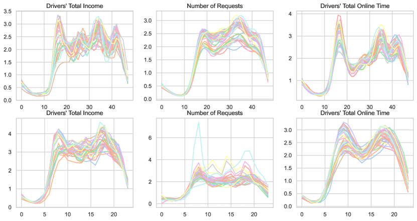
Figure 1: Scaled business metrics from City A (the first row) and City B (the second row) across 40 days, including drivers’ total income, the numbers of requests and drivers’ total online time.

We next discuss how to generate synthetic data based on the real datasets. The main idea is to fit the proposed L-TVCDP models to the real dataset and apply the parametric bootstrap to simulate the data. Let $\widetilde{\beta}_{0}({\tau})$, $\widetilde{\beta}({\tau})$, $\widetilde{\phi}_{0}({\tau})$, and $\widetilde{\Phi}({\tau})$ denote the smoothed estimators for $\beta_{0}({\tau})$, $\beta({\tau})$, $\phi_{0}({\tau})$ and $\Phi({\tau})$, respectively. We set $\widetilde{\gamma}({\tau})$ and $\widetilde{\Gamma}({\tau})$ to $(\delta/100)\times(\sum_{i,{\tau}}Y_{i,{\tau}}/nm)$ and $(\delta/100)\times(\sum_{i,{\tau}}S_{i,{\tau}}/nm)$, respectively. As such, the parameter $\delta$ controls the degree of the treatment effects. Specifically, the null holds if $\delta=0$ and the alternative holds if $\delta>0$. It corresponds to the increase relative to the outcome (state). We next generate the policies according to the temporal alternation design and simulate the responses and states based on the fitted model. Let TI denote the time span we implement each policy under the alternation design. For instance, if TI $=3$, then we first implements one policy for three hours, then switch to the other for another three hours and then switch back and forth between the two policies. We consider three choices of $n\in\{8,14,20\}$, fives choices of $\delta\in\{0,0.25,0.5,0.75,1\}$ and three choices of TI $\in\{1,3,6\}$. This corresponds to a total of 45 cases. The bandwidth is set $h=Cn^{-1/3}$, where $C$ is selected by the 5-fold cross validation method.

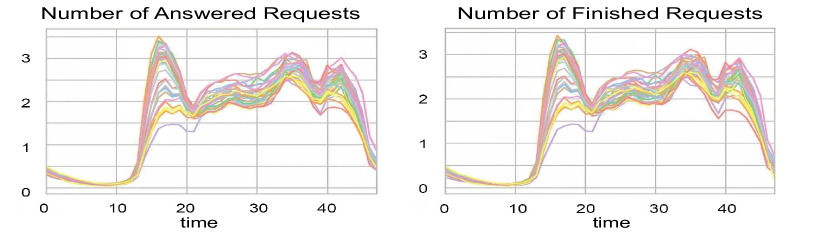
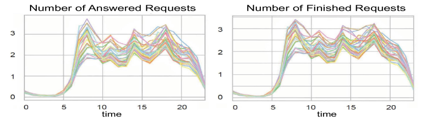
Figure 12: Scaled numbers of answered and finished requests from City A (the first row) and City B (the second row) across 40 days .

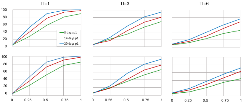
Figure 13: Empirical rejection rates of the proposed test for DE, with different combinations of $n,\delta,\textrm{TI}$ and outcomes based on the real dataset from city A (the number of answered requests in the first row and the number of finished requests in the second row).

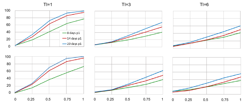
Figure 14: Empirical rejection rates of the proposed test for DE, with different combinations of $n,\delta,\textrm{TI}$ and outcomes based on the real dataset from city B (the number of answered requests in the first row and the number of finished requests in the second row).

In Figure 2, we depict the empirical rejection probabilities of the proposed test for DE, aggregated over 400 simulations, for all combinations. It can be seen that our test controls the type-I error and its power increases as $\delta$ increases. In addition, the empirical rejection rates decreases as TI increases. This phenomenon suggests that the more frequently we switch back and forth between the two policies, the more powerful the resulting test. It is due to the positive correlation between adjacent observations. To elaborate, consider the extreme case where we switch policies at each time. The policies assigned at any two adjacent time points are different. As such, the random effect cancels with each other, yielding an efficient estimator. We conduct some additional simulations using the numbers of answered requests and finished requests of cities A and B as responses (see Figure 12 in the supplement). Results are very similar and are reported in Figures 13–14 in the supplementary document. See also Tables 4–5 in the supplementary document.

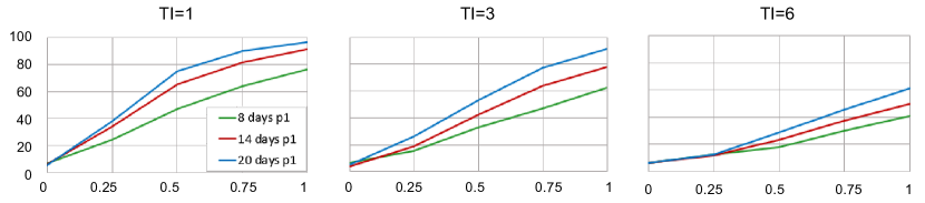
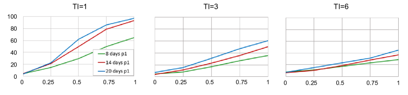
Figure 2: Simulation results for L-TVCDP: empirical rejection rates (expressed as percentages) of the proposed test for DE under different combinations of $(n,\delta,\textrm{TI})$ and types of outcomes. Synthetic data are simulated based on the real dataset from city A (the first row) and city B (the second row).

To infer IE, we set the outcome to drivers’ total online income. The empirical rejection probabilities of the proposed test for IE are reported in Figure 3. Results are aggregated over 400 simulations. Similarly, the proposed test is consistent. Its power increases with the sample size and $\delta$. In addition, its power under TI $=1$ is much larger than those under TI $=3$ or $6$. This suggests that we shall switch back and forth between the two policies as frequently as possible to maximize the power property of the test (see also Tables 6–7 in Supplementary document).

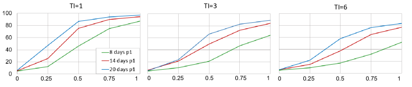
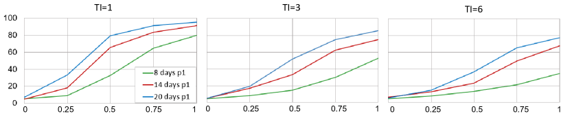
Figure 3: Simulation results for L-TVCDP: empirical rejection rates (expressed as percentages) of the proposed test for IE under different combinations of $(n,\delta,\textrm{TI})$. Synthetic data are simulated based on the real dataset from city A (the first row) and city B (the second row).

5.2 Spatio-temporal alternation design

To generate data under the spatio-temporal alternation design, we create a simulation environment based on the real dataset from city A. We divide the city into 10 non-overlapping regions. We plot these variables associated with 3 particular regions, over the first 10 days in Figure 4. It can be seen that although the daily trends differ across regions, the state and the response are highly correlated.

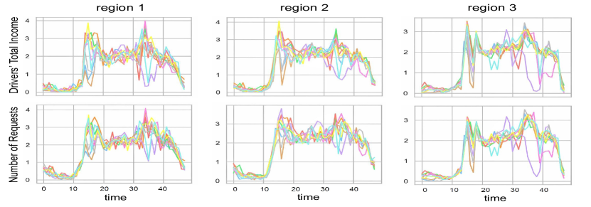
Figure 4: Number of call requests and drivers’ total income across different regions and days. The values are scaled for privacy concerns.

We fit the proposed models in (18) to the real dataset to estimate the varying coefficients and the variances of the random errors. Then we manually set the treatment effects $\widehat{\gamma}({\tau},\iota)$ and $\widehat{\Gamma}({\tau},\iota)$ to $(\delta_{1}/100)\times(\sum_{i=1}^{n}\sum_{{\tau}=1}^{m}Y_{i,{\tau},\iota}/nm)$ and $(\delta_{2}/100)\times(\sum_{i=1}^{n}\sum_{{\tau}=1}^{m}S_{i,{\tau},\iota}/nm)$ for some constants $\delta_{1}$ and $\delta_{2}>0$. We consider both the temporal and spatio-temporal alternation designs, and simulate the data via parametric bootstrap.

We also consider three choices of $n\in\{8,14,20\}$, three choices of TI $\in\{1,3,6\}$ and three choices of $\delta_{1},\delta_{2}\in\{0,0.5,1\}$. This yields a total of 81 combinations under each design. The rejection probabilities of the proposed tests for DE and IE tests are reported in Figures 5 and 6 (see also Tables 8 and 9 in the supplementary document). It can be seen that the type I error rates of the proposed test are close to the nominal level under both designs. More importantly, the power under spatio-temporal alternation design is higher than that of temporal alternation design in all cases. The reason is twofold. First, under the spatio-temporal design, we independently randomize the initial policy for each region, and adjacent regions may receive different policies. Observations across adjacent areas are likely to be positively correlated. As such, the variance of the estimated treatment effects will be smaller than that under the temporal design where all regions receive the same policy at each time. Second, we employ kernel smoothing twice when computing $\widehat{\textrm{DE}}_{st}$ and $\widehat{\textrm{IE}}_{st}$, as discussed in Section 3. This results in a more efficient estimator. In addition, compared with the results in Tables 4 and 6, it can be seen that the test that focuses on the entire city has better power property than the one that considers a particular region in general. Finally, the power decreases with TI and increases with $n$, $\delta_{1}$ and $\delta_{2}$.

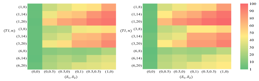
Figure 5: Simulation results for L-STVCDP: the empirical rejection probabilities of the proposed test test for DE under the temporal alternation design (left panel) and the spatio-temporal alternation design (right panel).

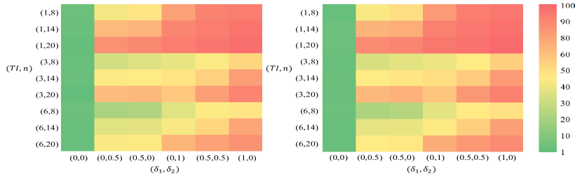
Figure 6: Simulation results for L-STVCDP: the empirical rejection probabilities of the proposed test test for IE under the temporal alternation design (left panel) and the spatio-temporal alternation design (right panel).

6 Real data analysis

In this section, we apply the proposed tests based on L-TVCDP and L-STVCDP to a number of real datasets from Didi Chuxing to examine the treatment effects of some newly developed order dispatch and vehicle reposition policies. Due to privacy, we do not publicize the names of these policies.

We first consider four data sets collected from four online experiments under the temporal alternation design. All the experiments last for 14 days. Policies are executed based on alternating half-hourly time intervals. We denote the cities, in which these experiments take place, as $C_{1},C_{2},$ $C_{3},$ and $C_{4}$ and their corresponding policies as $S_{1},S_{2},S_{3},$ and $S_{4}$, respectively. For each policy, we are interested in its effect on three key business metrics, including drivers’ total income, the answer rate, and the completion rate. Similar to Section 5.1, we use the number of call orders and drivers’ total online time to construct the time-varying state variables.

All the new policies are compared with some baseline policies in order to evaluate whether they improve some business outcomes. Specifically, in city $C_{1}$, policy $S_{1}$ is proposed to reduce the answer time (the time period between the time when an order is requested and the time when the order is responded by the driver). This in turn meets more call orders requests. Both policy $S_{2}$ in city $C_{2}$ and policy $S_{3}$ in city $C_{3}$ are designed to guide drivers to regions with more orders in order to reduce drivers’ idle time ratio. Policies $S_{2}$ and $S_{3}$ are designed to assign more drivers to areas with more orders. This in turn reduces drivers’ downtime and increase their income. Policy $S_{4}$ aims to balance drivers’ downtime and their average pick-up distance.

We also apply our test to another four datasets collected from four A/A experiments which compare the standard policy against itself. These A/A experiments are conducted two weeks before the A/B experiments. Each lasts for 14 days and thirty-minutes is defined as one time unit. We remark that the A/A experiment is employed as a sanity check for the validity of the proposed test. We expect our test will not reject the null when applied to these datasets, since the sole standard policy is used.

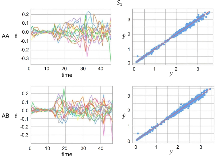
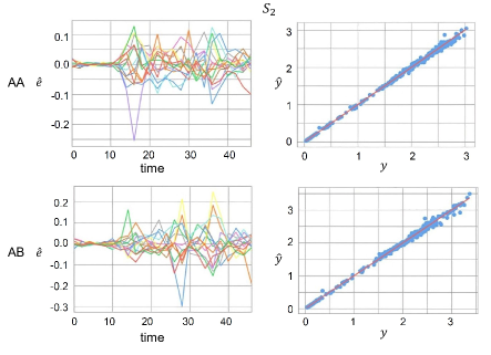
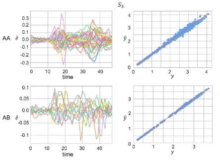
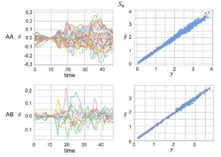
Figure 15: Plots of the fitted drivers’ total income against the observed values as well as the corresponding residuals. Data are collected from an A/A or A/B experiment under the temporal alternation design.

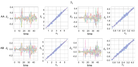
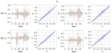
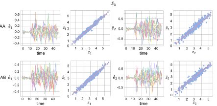
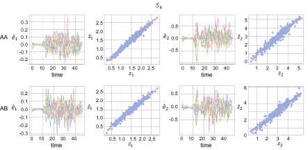
Figure 16: Plots of the fitted number of orders ($\widehat{e}_{1}$) and drivers’ online time ($\widehat{e}_{2}$) against their observed values, as well as the corresponding residuals. Data are collected from an A/A or A/B experiment under the temporal alternation design.

We fit the proposed L-TVCDP models to each of the eight datasets. In Figures 7 and 16, we plot the predicted outcomes against the observed values and plot the corresponding residuals over time for policy $S_{1}$. Results for policies $S_{2}$–$S_{4}$ are represented in Figure 15 in the supplementary article. It can be seen that the predicted outcomes are very close to the observed values, suggesting that the proposed model fits the data well. P-values of the proposed tests are reported in Tables 1 and 2. As expected, the proposed test does not reject the null hypothesis when applied to all datasets from A/A experiments. When applied to the data from A/B experiments, it can be seen that the new policy $S_{1}$ directly improves the answer rate and the completion rate, while increasing drivers’ total income in city $C_{1}$. It also significantly increases drivers’ income in the long run. Policy $S_{2}$ has significant direct and indirect effects on drivers’ income as expected. Policy $S_{4}$ significantly increases the immediate answer rate, while improving the overall passenger satisfaction. However, policy $S_{3}$ is not significantly better than the standard policy.

Table 1: One sided p-values of the proposed test for DE, when applied to eight datasets collected from the A/A or A/B experiment based on the temporal alternation design, with DTI, ART and CRT corresponding to drivers’ total income, the answer rate and the completion rate, respectively.

	AA			AB
	DTI(%)	ART(%)	CRT(%)	DTI(%)	ART(%)	CRT(%)
$S_{1}$	0.527	0.435	0.442	0.000	0.000	0.003
$S_{2}$	0.232	0.126	0.209	0.000	0.763	0.661
$S_{3}$	0.378	0.379	0.567	0.700	0.637	0.839
$S_{4}$	0.348	0.507	0.292	0.198	0.000	0.133

Table 2: One sided p-values of the proposed test for IE, when applied to eight datasets collected from the A/A or A/B experiment based on the temporal alternation design. Drivers’ total income is set to be the outcome of interest.

	S1		S2		S3		S4
	AA	AB	AA	AB	AA	AB	AA	AB
p-value	0.334	0.001	0.341	0.003	0.254	0.589	0.427	0.168

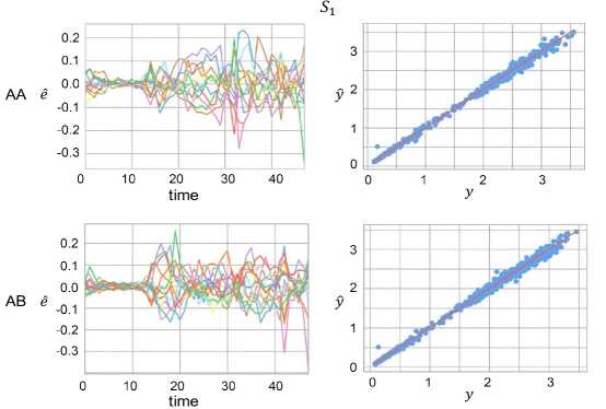
Figure 7: Plots of the fitted drivers’ total income against the observed values as well as the corresponding residuals. Data are collected from an A/A or A/B experiment under the temporal alternation design.

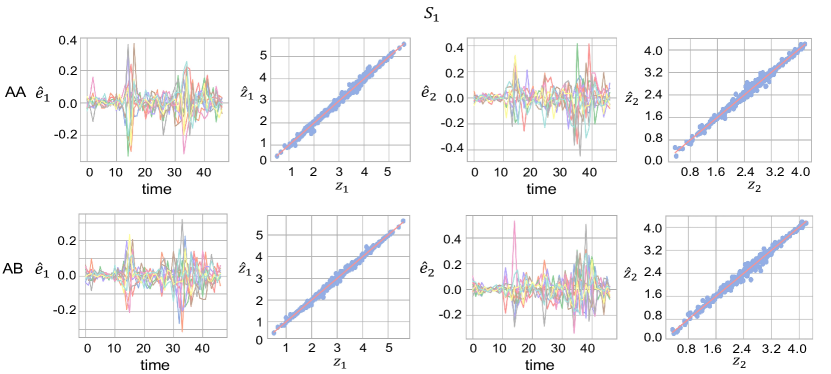
Figure 8: Plots of the fitted number of orders ($\widehat{e}_{1}$) and drivers’ online time ($\widehat{e}_{2}$) against their observed values, as well as the corresponding residuals. Data are collected from an A/A or A/B experiment under the temporal alternation design.

We further apply the proposed test to two real datasets collected from an A/A and A/B experiment under the spatio-temporal alternation design, conducted in city $C_{5}$. This city is partitioned into 17 regions. Within each region, more than 90% orders are answered by drivers in the same region. Similar to the temporal alternation design, both experiments last for 14 days and 30-minutes is set as one time unit. We take the number of requests as the state variables and drivers’ total income as the outcome, as in Section 5.2. In Figures 9 and 10, we plot the fitted drivers’ total income and the fitted number of requests against their observed values, and plot the corresponding residuals over time. We only present results associated with 2 regions in the city for space economy. The fitted values and residuals associated with other regions are similar and we do not present them to save space. It can be seen that the proposed models fit these datasets well. In addition, we report the p-values of the proposed test in Table 3. It can be seen that the new policy significantly increases drivers’ income. When applied to the dataset from the A/A experiment, it fails to reject either null hypothesis.

Table 3: One sided p-values of the proposed test, when applied to two datasets collected from the A/A or A/B experiment based on the spatio-temporal alternation design. Drivers’ total income is set to be the outcome of interest.

	DE		IE
	AA	AB	AA	AB
p-value	0.176	0.001	0.334	0.000

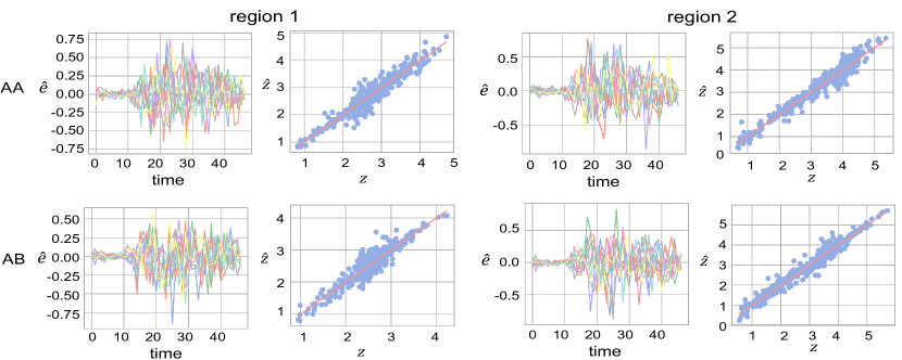
Figure 9: Plots of the fitted drivers’ income against the observed values, as well as the corresponding residuals. Data are collected from an A/A or A/B experiment under the spatio-temporal alternation design.

Figure 10: Plots of the fitted number of orders against the observed values, as well as the corresponding residuals. Data are collected from an A/A or A/B experiment under the spatio-temporal alternation design.

7 Discussion

In this study, driven by the need for policy evaluation in technological companies, we thoroughly examine AB testing for temporal and/or spatial dependent experiments, particularly in scenarios characterized by weak signals, (spatio)-temporal random effects, and intricate interference structures. Our approach offers two key benefits. Firstly, it accommodates the switchback design, which can significantly enhance testing power. As explained earlier, by applying diverse treatments to neighboring time points, we can potentially offset the impact of random effects at these times, resulting in more efficient estimations of treatment effects. Secondly, we break down the ATE into its DE and IE components. We then advocate for testing these effects separately. This separation aids decision-makers in gaining a clearer understanding of how different policies function and in devising more effective strategies and designs. Further details can be found in Section LABEL:sec:decomp of the supplementary document.

There are several intriguing avenues for future research. Firstly, considering Assumptions 1 and 2, it’s worth exploring scenarios where errors in the state regression model are not necessarily independent over time. This can be achieved by incorporating random effects into the state regression model, allowing for correlated errors over time. However, this introduces dependencies between these random effects, which in turn affects the conditional independence of past and future features. Consequently, the Markov assumption is violated, and applying existing OPE methods and our proposal from Section 2 directly would result in biased policy value estimations. In Section LABEL:sec:endogeneity of the supplementary document, we present two approaches to mitigate this endogeneity bias. Secondly, we can delve into situations involving a large number of state variables. However, in ride-sharing platforms, it’s reasonable to assume that the dimension of state variables is fixed. This typically involves a two-dimensional market feature, encompassing the number of call orders and the number of available drivers. We outline potential extensions to high-dimensional settings in Section LABEL:subsec:highd of the supplementary document. Thirdly, while the interference structure examined in this work is general, it remains relatively simple. It would be intriguing to explore more complex structural interferences across both space and time. Lastly, addressing statistical inference for deep neural networks remains an open challenge. This could represent a significant step toward incorporating deep learning into causal inference, offering promising directions for future research.

Appendix A Algorithms, Assumptions and Lemmas

Let $\widetilde{\bm{V}}_{\theta}({\tau}_{1},{\tau}_{2})$ and $\bm{V}_{\widetilde{\theta}}({\tau}_{1},{\tau}_{2})$ be the submatrices of $\widetilde{\bm{V}}_{\theta}$ and $\bm{V}_{\widetilde{\theta}}$, respectively, formed by rows in $\{({\tau}_{1}-1)(d+2)+1,({\tau}_{1}-1)(d+2)+2,\ldots,{\tau}_{1}(d+2)\}$ and columns in $\{({\tau}_{2}-1)(d+2)+1,({\tau}_{2}-1)(d+2)+2,\ldots,{\tau}_{2}(d+2)\}$. We first introduce some auxiliary lemmas.

Lemma 2

Under TCMIA and Assumptions 3 - 4, as $n,m\rightarrow\infty$, $h\rightarrow 0$, and $mh\rightarrow\infty$, we have $\sup_{{\tau}_{1},{\tau}_{2}}|\widetilde{\bm{V}}_{\theta}({\tau}_{1},{\tau}_{2})-\bm{V}_{\widetilde{\theta}}({\tau}_{1},{\tau}_{2})|=o_{p}(1)$.

Lemma 3

Under STCMIA, Assumptions 3 and 6, as $n,m,r\rightarrow\infty$, $h,h_{st}\rightarrow 0$ and $mh,rh_{st}\rightarrow\infty$, then $\sup_{{\tau}_{1},\iota_{1},{\tau}_{2},\iota_{2}}|\widetilde{\bm{V}}_{\theta,st}({\tau}_{1},\iota_{1},{\tau}_{2},\iota_{2})-\bm{V}_{\widetilde{\theta}_{st}}({\tau}_{1},\iota_{1},{\tau}_{2},\iota_{2})|=o_{p}(1)$.

We describe our inference procedure for DE under the spatio-temporal case here. A pseudocode summarizing our algorithm is given in Algorithm A. We denote for $\iota=1,\ldots,r$,

$$\bm{Y}_{i}={\mbox{diag}}\{Y_{i,1,1},\ldots,Y_{i,m,1},\ldots,Y_{i,1,r},\ldots,Y_{i,m,r}\},$$

$$\bm{Z}_{i}={\mbox{diag}}\{Z_{i,1,1}^{\top},\ldots,Z_{i,m,1}^{\top},\ldots,Z_{i,1,r}^{\top},\ldots,Z_{i,m,r}^{\top}\}.$$ (21)

Denote the longitude and latitude (scaled to be $[0,1]$) of region $\iota$ by $(u_{\iota},v_{\iota})$,

$$\displaystyle\kappa_{\ell,h_{st}}(\iota)=\frac{K\{(u_{\iota}-u_{\ell})/h_{st}\}K\{(v_{\iota}-v_{\ell})/h_{st}\}}{\sum_{j=1}^{r}K\{(u_{\iota}-u_{j})/h_{st}\}K\{(v_{\iota}-v_{j})/h_{st}\}}.$$ (22)

Let $\mathcal{K}=\mathcal{K}_{1}\mathcal{K}_{2}$, where $\mathcal{K}_{1}$ is a block matrix whose $(\iota,\ell)$th block is $\kappa_{\ell,h_{st}}(\iota)\bm{J}_{pm}$ for $1\leq\iota,\ell\leq r$ and $\mathcal{K}_{2}={\mbox{diag}}\{\Omega,\ldots,\Omega\}$. The estimation and inference procedure of DE in the spatio-temporal case is given as follows.

  Algorithm 3 Inference of DE under the spatio-temporal design

 

1:Compute $\widehat{\theta}_{st}^{0}({\tau},\iota)=\left(\sum_{i=1}^{n}Z_{i,{\tau},\iota}^{\top}Z_{i,{\tau},\iota}\right)^{-1}\left(\sum_{i=1}^{n}Z_{i,{\tau},\iota}^{\top}Y_{i,{\tau},\iota}\right)$ and $\widetilde{\theta}^{0}_{st}({\tau},\iota)=\sum_{j=1}^{m}\omega_{j,h}({\tau})\widehat{\theta}(j,\iota)$ for each ${\tau},\iota$.

2:Compute $\widetilde{\theta}_{st}({\tau},\iota)=\sum_{\ell=1}^{r}\kappa_{\ell,h_{st}}(\iota)\widetilde{\theta}({\tau},\ell)$.

3:Estimate the covariance $\Sigma_{y}$ by the following steps:  (i). estimate the combined noise by $\widehat{e}_{i,{\tau},\iota}=Y_{i,{\tau},\iota}-Z_{i,{\tau},\iota}^{\top}\widetilde{\theta}_{st}({\tau},\iota)$;  (ii). estimate the subject effects and measurement errors by

$$\widehat{\eta}_{i,{\tau},\iota}^{I}=\sum_{\ell=1}^{r}\kappa_{\ell,h_{st}}(\iota)\sum_{j=1}^{m}\omega_{j,h}({\tau})\widehat{e}_{i,j,\ell},\quad\widehat{\eta}_{i,{\tau},\iota}^{II}=\sum_{\ell=1}^{r}\kappa_{\ell,h_{st}}(\iota)\widehat{e}_{i,j,\ell}-\widehat{\eta}_{i,{\tau},\iota}^{I},$$

$$\widehat{\eta}_{i,{\tau},\iota}^{III}=\sum_{j=1}^{m}\omega_{j,h}({\tau})\widehat{e}_{i,j,\ell}-\widehat{\eta}_{i,{\tau},\iota}^{I},\quad\widehat{\varepsilon}_{i,{\tau},\iota}=\widehat{e}_{i,{\tau},\iota}-\widehat{\eta}_{i,{\tau},\iota}^{I}-\widehat{\eta}_{i,{\tau},\iota}^{II}-\widehat{\eta}_{i,{\tau},\iota}^{III}.$$ (23)

 (iii). the covariances of $\eta$ and $\varepsilon$ are estimated by

$$\widehat{\Sigma}_{\eta^{I}}({\tau}_{1},\iota_{1},{\tau}_{2},\iota_{2})=\frac{1}{n-1}\sum_{i=1}^{n}\widehat{\eta}_{i,{\tau}_{1},\iota_{1}}^{I}\widehat{\eta}_{i,{\tau}_{2},\iota_{2}}^{I},\quad\widehat{\Sigma}_{\eta^{II}}({\tau}_{1},\iota_{1},{\tau}_{2})=\frac{1}{n-1}\sum_{i=1}^{n}\widehat{\eta}_{i,{\tau}_{1},\iota_{1}}^{II}\widehat{\eta}_{i,{\tau}_{2},\iota_{1}}^{II},$$

$$\widehat{\Sigma}_{\eta^{III}}({\tau}_{1},\iota_{1},\iota_{2})=\frac{1}{n-1}\sum_{i=1}^{n}\widehat{\eta}_{i,{\tau}_{1},\iota_{1}}^{III}\widehat{\eta}_{i,{\tau}_{1},\iota_{2}}^{III},\quad\widehat{\sigma}_{\varepsilon}^{2}({\tau}_{1},\iota_{1})=\frac{1}{n-1}\sum_{i=1}^{n}\widehat{\varepsilon}_{i,{\tau}_{1},\iota_{1}}^{2};$$ (24)

 (iv). the covariance of outcome is estimated by

$$\widehat{\Sigma}_{y}({\tau}_{1},\iota_{1},{\tau}_{2},\iota_{2})= \widehat{\Sigma}_{\eta^{I}}({\tau}_{1},\iota_{1},{\tau}_{2},\iota_{2})+\widehat{\Sigma}_{\eta^{II}}({\tau}_{1},\iota_{1},{\tau}_{2})I(\iota_{1}=\iota_{2})$$

$$+\widehat{\sigma}_{\varepsilon^{I}}^{2}({\tau}_{1},\iota_{1},\iota_{2})I({\tau}_{1}={\tau}_{2})+\widehat{\sigma}_{\varepsilon^{II}}^{2}({\tau}_{1},\iota_{1})I({\tau}_{1}={\tau}_{2},\iota=\iota_{2}).$$

4:Compute

$$\widehat{\bm{V}}_{\theta_{st}}=\left\{\sum_{i=1}^{n}\bm{Z}_{i}^{\top}\bm{Z}_{i}\right\}^{-1}\left\{\sum_{i=1}^{n}\bm{Z}_{i}^{\top}\widehat{\bm{\Sigma}}^{-1}\bm{Z}_{i}\right\}\left\{\sum_{i=1}^{n}\bm{Z}_{i}^{\top}\bm{Z}_{i}\right\}^{-1}$$

where $\widehat{\bm{\Sigma}}=\{\widehat{\Sigma}_{y}({\tau}_{1},\iota_{1},{\tau}_{2},\iota_{2})\}_{{\tau}_{1},\iota_{1},{\tau}_{2},\iota_{2}}$ and $\widetilde{\bm{V}}_{\theta_{st}}=\mathcal{K}\widehat{\bm{V}}_{\theta_{st}}\mathcal{K}^{\top}$.

5:Calculate $\widehat{\textrm{DE}}_{st}$ and the standard error $\widehat{se}(\widehat{\textrm{DE}}_{st})$ based on $\widetilde{\bm{V}}_{\theta_{st}}$.

6:Reject $H_{0}^{DE}$ if $\widehat{\textrm{DE}}_{st}/\widehat{se}(\widehat{\textrm{DE}}_{st})$ exceeds the upper $\alpha$th quantile of a standard normal distribution.

 

  Algorithm 4 Inference of IE under the spatio-temporal design

 

1:Compute the OLS estimator

$$\widehat{\bm{\Theta}}=\left\{\sum_{i=1}^{n}\bm{Z}_{i,(-m)}\bm{Z}_{i,(-m)}^{\top}\right\}^{-1}\left\{\sum_{i=1}^{n}\bm{Z}_{i,(-m)}\bm{S}_{i,(-1)}^{\top}\right\}.$$

2:Compute ${\widetilde{\Theta}_{st}=\mathcal{K}\widetilde{\Theta}}$.

3:Plug-in the parameter estimates $\widetilde{\Theta}_{st}$ and $\widetilde{\theta}_{st}$ to obtain $\widehat{\textrm{IE}}_{st}$.

4:Compute the residuals $\widehat{E}_{i,{\tau},\iota}=S_{i,{\tau},\iota}-Z_{i,{\tau},\iota}^{\top}\widetilde{\Theta}({\tau},\iota)$.

5:for $b=1,\ldots,B$ do

6:generate i.i.d. standard normal random variables $\{\xi_{i}^{b}\}_{i=1}^{n}$;

7:generate pseudo outcomes $S_{i,{\tau},\iota}^{b}$ and $Y_{i,{\tau},\iota}^{b}$ by $S_{i,{\tau}+1,\iota}^{b}=Z_{i,{\tau},\iota}\widetilde{\Theta}({\tau},\iota)+\xi_{i}\widehat{E}_{i,{\tau},\iota}$ and $Y_{i,{\tau},\iota}^{b}=Z_{i,{\tau},\iota}\widetilde{\theta}_{st}({\tau},\iota)+\xi\widehat{e}_{i,{\tau},\iota}$, where $Z_{i,{\tau},\iota}^{b}=\{1,(S_{i,{\tau},\iota}^{b})^{\top},A_{i,{\tau},\iota},\bar{A}_{i,{\tau},\mathcal{N}_{\iota}}\}^{\top}$;

8:substitute $Y_{i,{\tau},\iota}$ and $S_{i,{\tau},\iota}$ with $Y_{i,{\tau},\iota}^{b}$ and $S_{i,{\tau},\iota}^{b}$, and repeat the procedures in Steps 1-3 to obtain the plug-in estimator $\widehat{\textrm{IE}}_{st}^{b}$.

9:end for

10:Reject $H_{0}^{IE}$ if $\widehat{\textrm{IE}}_{st}$ exceeds the upper $\alpha$th empirical quantile of $\{\widehat{\textrm{IE}}_{st}^{b}-\widehat{\textrm{IE}}_{st}\}_{b}$.

 

Appendix B Proof of Lemma 1

We first prove (4). It follows from the law of total expectation that

$${\mathbb{E}}(Y_{{\tau}}|\bar{A}_{{\tau}},\bar{S}_{{\tau}})={\mathbb{E}}^{\bar{Y}_{{\tau}-1}|\bar{A}_{{\tau}},\bar{S}_{{\tau}}}\{{\mathbb{E}}(Y_{{\tau}}|\bar{A}_{{\tau}},\bar{S}_{{\tau}},\bar{Y}_{{\tau}-1})\},$$

where $\bar{A}_{{\tau}}$, $\bar{S}_{{\tau}}$ and $\bar{Y}_{{\tau}-1}$ denote the history of actions, states and outcomes, respectively. The first expectation on the right-hand-side (RHS) is taken with respect to the conditional distribution of $\bar{Y}_{{\tau}-1}$ given that $(\bar{A}_{{\tau}},\bar{S}_{{\tau}})$.

Without loss of generality, assume both the outcome and the state are discrete. Let $p^{\bar{Y}_{{\tau}-1}|\bar{A}_{{\tau}},\bar{S}_{{\tau}}}$ denotes the conditional probability mass function of $\bar{Y}_{{\tau}-1}$ given $\bar{A}_{{\tau}},\bar{S}_{{\tau}}$, we have

$${\mathbb{E}}(Y_{{\tau}}|\bar{A}_{{\tau}}=\bar{a}_{{\tau}},\bar{S}_{{\tau}}=\bar{s}_{{\tau}})=\sum_{\bar{y}_{{\tau}-1}}p^{\bar{Y}_{{\tau}-1}|\bar{A}_{{\tau}}=\bar{a}_{{\tau}},\bar{S}_{{\tau}}=\bar{s}_{{\tau}}}(\bar{y}_{\tau-1})\{{\mathbb{E}}(Y_{{\tau}}|\bar{A}_{{\tau}}=\bar{a}_{{\tau}},\bar{S}_{{\tau}}=\bar{s}_{{\tau}},\bar{Y}_{{\tau}-1}=\bar{y}_{{\tau}-1})\}.$$

According to CA, the second term on the RHS is equal to

$${\mathbb{E}}[Y_{{\tau}}^{*}(\bar{a}_{{\tau}})|\bar{A}_{{\tau}}=\bar{a}_{{\tau}},\bar{S}_{{\tau}}^{*}(\bar{a}_{{\tau}-1})=\bar{s}_{{\tau}},\bar{Y}_{{\tau}-1}^{*}(\bar{a}_{{\tau}-1})=\bar{y}_{{\tau}-1}],$$

where $\bar{S}_{{\tau}}^{*}(\bar{a}_{t-1})$ and $\bar{Y}_{{\tau}-1}^{*}(\bar{a}_{{\tau}-1})$ denote the sets of potential states and outcomes up to time ${\tau}$ and ${\tau}-1$, respectively. It follows that

$${\mathbb{E}}(Y_{{\tau}}|\bar{A}_{{\tau}}=\bar{a}_{{\tau}},\bar{S}_{{\tau}}=\bar{s}_{{\tau}})=\sum_{\bar{y}_{{\tau}-1}}p^{\bar{Y}_{{\tau}-1}|\bar{A}_{{\tau}}=\bar{a}_{{\tau}},\bar{S}_{{\tau}}=\bar{s}_{{\tau}}}(\bar{y}_{\tau-1})\{{\mathbb{E}}[Y_{{\tau}}^{*}(\bar{a}_{{\tau}})|\bar{A}_{{\tau}}=\bar{a}_{{\tau}},\bar{S}_{{\tau}}^{*}(\bar{a}_{{\tau}-1})=\bar{s}_{{\tau}},\bar{Y}_{{\tau}-1}^{*}(\bar{a}_{{\tau}-1})=\bar{y}_{{\tau}-1}]\}.$$

Under SRA and PA, the conditional expectation on the right-hand-side is independent of the actions. In addition, it is equal to $R_{{\tau}}(\bar{a}_{{\tau}},\bar{s}_{{\tau}})$, independent of $\bar{y}_{{\tau}-1}$. This yields (4).

We next show (5). Using similar arguments, we can show that

$${\mathbb{E}}\{R_{{\tau}}(a_{{\tau}},S_{{\tau}}^{*}(\bar{a}_{{\tau}-1}),\cdots,S_{1})\}={\mathbb{E}}[{\mathbb{E}}\{R_{{\tau}}(a_{{\tau}},S_{{\tau}}^{*}(\bar{a}_{{\tau}-1}),\cdots,S_{1})|A_{1}=a_{1},\bar{S}_{{\tau}-1}^{*}(\bar{a}_{{\tau}-2}),\bar{Y}_{{\tau}-1}^{*}(\bar{a}_{{\tau}-1})\}].$$

Under CA, we can replace $Y_{1}^{*}(a_{1})$ and $S_{2}^{*}(a_{1})$ with $Y_{1}$ and $S_{2}$, respectively. Under SRA and PA, the event $A_{2}=a_{2}$ can be included in the conditioning set. This yields that

$${\mathbb{E}}\{R_{{\tau}}(a_{{\tau}},S_{{\tau}}^{*}(\bar{a}_{{\tau}-1}),\cdots,S_{1})\}$$

$$= {\mathbb{E}}[{\mathbb{E}}\{R_{{\tau}}(a_{{\tau}},S_{{\tau}}^{*}(\bar{a}_{{\tau}-1}),\cdots,A_{1},S_{1})|A_{2}=a_{2},A_{1}=a_{1},\bar{S}_{{\tau}-1}^{*}(\bar{a}_{{\tau}-2}),\bar{Y}_{{\tau}-1}^{*}(\bar{a}_{{\tau}-1}),S_{1},Y_{1}\}].$$

Iteratively applying this argument allows us to repeatedly replace the counterfactual variables with the observed ones. At the end, all the potential outcomes/states will be replaced with the observed versions conditional on the actions. The proof is hence completed.

Appendix C Proof of Proposition 1

Recall that

$$\textrm{DE}=\sum_{{\tau}=1}^{m}{\mathbb{E}}\{R_{{\tau}}(1,S_{\tau}^{*}(\bm{0}_{{\tau}-1}),0,S_{{\tau}-1}^{*}(\bm{0}_{{\tau}-2}),\ldots,S_{1})-R_{\tau}(0,S_{\tau}^{*}(\bm{0}_{{\tau}-1}),0,S_{{\tau}-1}^{*}(\bm{0}_{{\tau}-2}),\ldots,S_{1})\},$$

$$\textrm{IE}=\sum_{{\tau}=1}^{m}{\mathbb{E}}\{R_{{\tau}}(1,S_{\tau}^{*}(\bm{1}_{{\tau}-1}),1,S_{{\tau}-1}^{*}(\bm{1}_{{\tau}-2}),\ldots,S_{1})-R_{\tau}(1,S_{\tau}^{*}(\bm{0}_{{\tau}-1}),0,S_{{\tau}-1}^{*}(\bm{0}_{{\tau}-2}),\ldots,S_{1})\}.$$

Under Model 1, each summand in DE equals $\gamma({\tau})$. It follows that

$$\textrm{DE}=\sum_{{\tau}=1}^{m}\gamma({\tau}).$$

Similarly, for IE, we have

$${\mathbb{E}}\{R_{{\tau}}(1,S_{\tau}^{*}(\bm{1}_{{\tau}-1}),1,S_{{\tau}-1}^{*}(\bm{1}_{{\tau}-2}),\ldots,S_{1})-R_{\tau}(1,S_{\tau}^{*}(\bm{0}_{{\tau}-1}),0,S_{{\tau}-1}^{*}(\bm{0}_{{\tau}-2}),\ldots,S_{1})\}$$

$$= {\mathbb{E}}\{\beta_{0}({\tau})+S_{\tau}^{*}(\bm{1}_{{\tau}-1})^{\top}\beta({\tau})+\gamma({\tau})\}-{\mathbb{E}}\{\beta_{0}({\tau})+S_{\tau}^{*}(\bm{0}_{{\tau}-1}))^{\top}\beta({\tau})+\gamma({\tau})\}$$

$$= {\mathbb{E}}\{S_{\tau}^{*}(\bm{1}_{{\tau}-1})-S_{\tau}^{*}(\bm{0}_{{\tau}-1})\}^{\top}\beta({\tau})$$

$$= {\mathbb{E}}[\Phi({\tau}-1)\{S_{{\tau}-1}^{*}(\bm{1}_{{\tau}-2})-S_{{\tau}-1}^{*}(\bm{0}_{{\tau}-2})\}+\Gamma({\tau}-1)]^{\top}\beta({\tau})$$

$$= {\mathbb{E}}[\Phi({\tau}-1)\Phi({\tau}-2)\{S_{{\tau}-2}^{*}(\bm{1}_{{\tau}-3})-S_{{\tau}-2}^{*}(\bm{0}_{{\tau}-3})\}+\Phi({\tau}-1)\Gamma({\tau}-2)+\Gamma({\tau}-1)]^{\top}\beta({\tau})$$

$$\cdots$$

$$= \beta({\tau})^{\top}\left\{\sum_{k=1}^{{\tau}-1}\left(\prod_{l=k+1}^{{\tau}-1}\Phi(l)\right)\Gamma(k)\right\},$$

which completes the proof.

Appendix D Proofs of Lemmas 2 and 3

The proof of Lemma 3 is similar to that of Lemma 2. Hence, we focus on proving Lemma 2 for space economy.

Proof : We first prove that $\sup_{{\tau}_{1},{\tau}_{2}}|\widehat{\Sigma}_{y}({\tau}_{1},{\tau}_{2})-\Sigma_{y}({\tau}_{1},{\tau}_{2})|=o_{p}(1)$. It suffices to show that $n^{-1}\sum_{i=1}^{n}\widehat{\eta}_{i,{\tau}_{1}}\widehat{\eta}_{i,{\tau}_{2}}$ and $n^{-1}\sum_{i=1}^{n}\widehat{\varepsilon}_{i,{\tau}}^{2}$ are consistent estimators of $\Sigma_{\eta}({\tau}_{1},{\tau}_{2})$ and $\sigma_{\varepsilon,{\tau}}^{2}$. According to Section 2.2, we have $\widehat{e}_{i,{\tau}}=Y_{i,{\tau}}-Z_{i,{\tau}}^{\top}\widetilde{\theta}({\tau})$. Notice that

$$\widehat{\eta}_{i,{\tau}}=\sum_{j=1}^{m}\omega_{j,h}({\tau})\widehat{e}_{i}(j).$$

We follow notations in Zhu et al. (2014) and write

$$\bar{\varepsilon}_{i,{\tau}}=\sum_{j=1}^{m}\omega_{j,h}({\tau})\varepsilon_{i,j},\quad\Delta_{K}\eta_{i,{\tau}}=\sum_{j=1}^{m}\omega_{j,h}({\tau})\left\{\eta_{i,j}-\eta_{i,{\tau}}\right\},$$

$$\Delta_{K}\theta({\tau})=\sum_{j=1}^{m}\omega_{j,h}({\tau})\left\{\theta(j)-\widehat{\theta}(j)\right\},\quad\Delta_{\eta_{i}}({\tau})=\bar{\varepsilon}_{i,{\tau}}+\Delta_{K}\eta_{i,{\tau}}+Z_{i,{\tau}}^{\top}\Delta_{K}\theta({\tau}).$$

Then we have

$$\widehat{\eta}_{i,{\tau}}-{\eta}_{i,{\tau}}=\Delta_{\eta_{i}}({\tau}),$$

which gives

$$n^{-1}\sum_{i=1}^{n}\widehat{\eta}_{i,{\tau}_{1}}\widehat{\eta}_{i,{\tau}_{2}}\,=\, n^{-1}\sum_{i=1}^{n}\eta_{i,{\tau}_{1}}\eta_{i,{\tau}_{2}}+n^{-1}\sum_{i=1}^{n}\Delta_{\eta_{i}}({\tau}_{1})\Delta_{\eta_{i}}({\tau}_{2})$$

$$+n^{-1}\sum_{i=1}^{n}\eta_{i,{\tau}_{1}}\Delta_{\eta_{i}}({\tau}_{2})+n^{-1}\sum_{i=1}^{n}\Delta_{\eta_{i}}({\tau}_{1})\eta_{i,{\tau}_{2}}.$$

The first term $n^{-1}\sum_{i=1}^{n}\eta_{i,{\tau}_{1}}\eta_{i,{\tau}_{2}}$ converges to $\Phi_{\eta}({\tau}_{1},{\tau}_{2})$ according to the Law of Large Number. We next show

• $I_{1}=n^{-1}\sum_{i=1}^{n}\Delta_{\eta_{i}}({\tau}_{1})\Delta_{\eta_{i}}({\tau}_{2})$ converges to zero for any $({\tau}_{1},{\tau}_{2})\in\mathcal{T}^{2}$.

• $I_{2}=n^{-1}\sum_{i=1}^{n}\eta_{i,{\tau}_{1}}\Delta_{\eta_{i}}({\tau}_{2})+n^{-1}\sum_{i=1}^{n}\Delta_{\eta_{i}}({\tau}_{1})\eta_{i,{\tau}_{2}}$ converges to zero for any $({\tau}_{1},{\tau}_{2})\in\mathcal{T}^{2}$.

By mutually multiplying the three terms in the summation form of $\Delta_{\eta_{i}}({\tau})$, we have

$$I_{1} =n^{-1}\sum_{i=1}^{n}\bar{\varepsilon}_{i,{\tau}_{1}}\bar{\varepsilon}_{i,{\tau}_{2}}+n^{-1}\sum_{i=1}^{n}\Delta_{K}\eta_{i,{\tau}}\Delta_{K}\eta_{i,{\tau}_{2}}+n^{-1}\sum_{i=1}^{n}Z_{i,{\tau}_{1}}^{\top}\Delta_{K}\theta({\tau}_{1})\Delta_{K}\theta({\tau}_{2})^{\top}Z_{i,{\tau}_{2}}$$

$$+n^{-1}\sum_{i=1}^{n}\bar{\varepsilon}_{i,{\tau}_{1}}\Delta_{K}\eta_{i}({\tau}_{2})+n^{-1}\sum_{i=1}^{n}\Delta_{K}\eta_{i,{\tau}_{1}}\bar{\varepsilon}_{i,{\tau}_{2}}+n^{-1}\sum_{i=1}^{n}\bar{\varepsilon}_{i,{\tau}_{1}}\Delta_{K}\theta({\tau}_{2})^{\top}Z_{i,{\tau}_{2}}$$

$$+n^{-1}\sum_{i=1}^{n}Z_{i,{\tau}_{1}}^{\top}\Delta_{K}\theta({\tau}_{1})\bar{\varepsilon}_{i,{\tau}_{2}}+n^{-1}\sum_{i=1}^{n}\Delta_{K}\eta_{i,{\tau}_{1}}\Delta_{K}\theta({\tau}_{2})^{\top}Z_{i,{\tau}_{2}}+n^{-1}\sum_{i=1}^{n}Z_{i,{\tau}_{1}}^{\top}\Delta_{K}\theta(1)\Delta_{K}\eta_{i,{\tau}_{2}}$$

By the independence between $\varepsilon_{i,{\tau}_{1}}$ and $\varepsilon_{i,{\tau}_{2}}$, the first term $n^{-1}\sum_{i=1}^{n}\bar{\varepsilon}_{i,{\tau}_{1}}\bar{\varepsilon}_{i,{\tau}_{2}}$ converges to zero. As for the second term, using standard arguments in establishing theoretical properties of kernel estimators, the bias term satisfies ${\mathbb{E}}\sum_{j=1}^{m}\omega_{j,h}({\tau})\left\{\eta_{i,j}-\eta_{i,{\tau}}\right\}=O(h^{2}+m^{-1})$, whereas the variance term satisfies ${\mbox{Var}}[\sum_{j=1}^{m}\omega_{j,h}({\tau})\left\{\eta_{i,j}-\eta_{i,{\tau}}\right\}]=O(m^{-\textbf{}1}h^{-1})$. It follows that

$$n^{-1}\sum_{i=1}^{n}\Delta_{K}\eta_{i,{\tau}_{1}}\Delta_{K}\eta_{i,{\tau}_{2}}$$

$$= n^{-1}\sum_{i=1}^{n}\left[\sum_{j=1}^{m}\omega_{j,h}({\tau}_{1})\left\{\eta_{i,j}-\eta_{i,{\tau}_{1}}\right\}\right]\left[\sum_{j=1}^{m}\omega_{j,h}({\tau}_{2})\{\eta_{i,j}-\eta_{i,{\tau}_{2}}\}\right]$$

$$= O_{p}(h^{4}+m^{-1}h^{-1}).$$

As for the third term, notice that $\left\{\widehat{\theta}({\tau})-\theta({\tau}):{\tau}\right\}$ converges uniformly to zero, $\left\{\Delta_{K}\theta({\tau}):{\tau}\right\}$ converges uniformly to zero as well. Under the given conditions, $n^{-1}\sum_{i=1}^{n}Z_{i,{\tau}_{1}}^{\top}Z_{i,{\tau}_{2}}$ is $O_{p}(1)$. It follows that the third term is $o_{p}(1)$. The remaining six cross products converges to zero according to the Law of Large Number and the mutual independence of $Z_{i}$, $\varepsilon_{i}$, and $\eta_{i}$ imposed in Assumption 4 . This completes the proof of (a).

To prove (b), we only need to prove $n^{-1}\sum_{i=1}^{n}\eta_{i,{\tau}_{1}}\Delta_{K}\eta_{i,{\tau}_{2}}=o_{p}(1)$ since that $\eta_{i}$ is independent of $Z_{i}$ and $\varepsilon_{i}$. This follows from the fact that

$$n^{-1}\sum_{i=1}^{n}\eta_{i,{\tau}_{1}}\left[\sum_{j=1}^{m}\omega_{j,h}({\tau}_{2})\{\eta_{i,j}-\eta_{i,{\tau}_{2}}\}\right]$$

$$= \sum_{j=1}^{m}\omega_{j,h}({\tau}_{2})n^{-1}\left\{\sum_{i=1}^{n}\eta_{i,j}\eta_{i,{\tau}}-\sum_{i=1}^{n}\eta_{i,{\tau}_{1}}\eta_{i,{\tau}_{2}}\right\}$$

$$= \sum_{j=1}^{m}\omega_{j,h}({\tau}_{2})\{\Sigma_{\eta}(j,{\tau}_{1})-\Sigma_{\eta}(t,{\tau}_{2})\}+o_{p}(1),$$ (25)

where the first two term on the right hand of (D) is $O(h^{2})$ according to the assumption on the distribution of $\eta_{i,{\tau}}$; see the equation (26) in the supplementary materials of Zhu et al. (2014).

We next prove the consistency of $n^{-1}\sum_{i=1}^{n}\widehat{\varepsilon}_{i,{\tau}}^{2}$. Notice that

$$\widehat{\varepsilon}_{i,{\tau}}=\widehat{e}_{i,{\tau}}-\widehat{\eta}_{i,{\tau}}=y_{i,{\tau}}-Z_{i,{\tau}}^{\top}\widehat{\theta}({\tau})-\widehat{\eta}_{i,{\tau}}.$$

Similarly to the proof of (a), we denote $\Delta_{\theta}({\tau})=\widehat{\theta}({\tau})-\theta({\tau})$, and $\Delta_{\varepsilon_{i}}({\tau})=-Z_{i,{\tau}}^{\top}\Delta_{\theta}({\tau})-\Delta_{\eta_{i}}({\tau})$. It follows that

$$n^{-1}\sum_{i=1}^{n}\widehat{\varepsilon}_{i,{\tau}}^{2}=n^{-1}\sum_{i=1}^{n}\varepsilon_{i,{\tau}}^{2}+n^{-1}\sum_{i=1}^{n}\Delta_{\varepsilon_{i}}^{2}({\tau})+2n^{-1}\sum_{i=1}^{n}\varepsilon_{i,{\tau}}\Delta_{\varepsilon_{i}}^{2}({\tau}).$$

The first term $n^{-1}\sum_{i=1}^{n}\varepsilon_{i,{\tau}}^{2}$ converges to $\sigma_{\varepsilon}^{2}({\tau})$ according to the Law of Large Number, and the other two terms both converge to zero based on the same arguments used before. We omit the details to save space.

Finally, recall that $\widehat{\bm{V}}_{\theta}$ is the sandwich estimator of $\bm{V}_{\widehat{\theta}}$ defined in (13). It is straightforward to show that $\sup_{{\tau}_{1},{\tau}_{2}}|\widehat{\bm{V}}_{\theta}({\tau}_{1},{\tau}_{2})-\bm{V}_{\widehat{\theta}}({\tau}_{1},{\tau}_{2})|=o_{p}(1)$ based on $\sup_{{\tau}_{1},{\tau}_{2}}|\widehat{\Sigma}_{y}({\tau}_{1},{\tau}_{2})-\Sigma_{y}({\tau}_{1},{\tau}_{2})|=o_{p}(1)$. Similarly, we can derive that $\sup_{{\tau}_{1},{\tau}_{2}}|\widetilde{\bm{V}}({\tau}_{1},{\tau}_{2})-\bm{V}_{\widetilde{\theta}}({\tau}_{1},{\tau}_{2})|=o_{p}(1)$. We omit the details to save space. $\square$

Appendix E Proof of Theorem 1

Proof : Argument (i) in Theorem 1 can be directly proven based on the properties of the ordinary least square estimator. We focus on proving Argument (ii). Notice that $\widetilde{\theta}({\tau})$ can essentially rewritten as a linear combination of $\{\widehat{\theta}(k)\}_{k}$, i.e.,

$$\widetilde{\theta}({\tau}) =\sum_{k=1}^{m}\omega_{k,h}({\tau})\widehat{\theta}(k)=\sum_{k=1}^{m}\omega_{k,h}({\tau})\{\widehat{\theta}(k)-\theta(k)+\theta(k)-\theta({\tau})+\theta({\tau})\}$$

$$=\theta({\tau})+\sum_{k=1}^{m}\omega_{k,h}({\tau})\{\widehat{\theta}(k)-\theta(k)\}+\sum_{k=1}^{m}\omega_{k,h}({\tau})\{\theta(k)-\theta({\tau})\}.$$

It follows that

$$E\{\widetilde{\theta}(\tau)-\theta(\tau)\}$$

$$= \sum_{k=1}^{m}\omega_{k,h}(\tau)\{\widehat{\theta}(k)-\theta(\tau)\}$$

$$= \sum_{k=1}^{m}\omega_{k,h}(\tau)\{\theta(k)-\theta(\tau)\}$$

$$= \left\{\sum_{k=1}^{m}\frac{1}{mh}K\left(\frac{\tau-k}{mh}\right)\right\}^{-1}\cdot\left[\sum_{k=1}^{m}\frac{1}{mh}K\left(\frac{\tau-k}{mh}\right)\{\theta(k)-\theta(\tau)\}\right]$$

Denote

$${f}(\tau)=\sum_{k=1}^{m}\frac{1}{mh}K\left(\frac{\tau-k}{mh}\right)$$

$${g}_{1}(\tau)=\sum_{k=1}^{m}\frac{1}{mh}K\left(\frac{\tau-k}{mh}\right)\{\theta(k)-\theta(\tau)\}$$

Note that $f(\tau){\longrightarrow}1$, it suffices to bound $|{g}_{1}(\tau)|$. Define

$${g}_{2}(\tau)=\int_{0}^{1}\frac{1}{h}K\left(\frac{um-\tau}{mh}\right)\{\theta(um)-\theta(\tau)\}du.$$

By decomposing ${g}_{1}(\tau)={g}_{2}(\tau)+\left\{{g}_{1}(\tau)-{g}_{2}(\tau)\right\}$, we first show ${g}_{2}(\tau)=O\left(h^{2}\right)$, and then prove ${g}_{1}(\tau)-{g}_{2}(\tau)=O\left(m^{-1}\right)$. The time domain of interest is fixed, and the increment of $m$ equals the encryption of grids. Define a function $\theta_{0}$ such that $\theta_{0}(\cdot)$ such that $\theta(\tau)=\theta_{0}\left(\frac{\tau}{m}\right)$ for any $\tau$. It follows that

$$\theta(s)-\theta(t)=\theta_{0}\left(\frac{s}{m}\right)-\theta_{0}\left(\frac{t}{m}\right)=\theta_{0}^{\prime}\left(\frac{t}{m}\right)\left(\frac{s-t}{m}\right)+\frac{1}{2}\theta_{0}^{\prime\prime}\left(\frac{t}{m}\right)\left(\frac{s-t}{m}\right)^{2}+O\left(m^{-3}\right).$$

Then we have

$${g}_{2}(\tau) =\int_{0}^{1}\frac{1}{h}K\left(\frac{u-\tau/m}{h}\right)\left\{\theta_{0}(u)-\theta_{0}\left(\frac{\tau}{m}\right)\right\}du$$

$$=\int_{0}^{1}\frac{1}{h}K\left(\frac{u-\tau/m}{h}\right)\left\{\theta_{0}^{\prime}\left(\frac{\tau}{m}\right)\left(u-\frac{\tau}{m}\right)+\theta_{0}^{\prime\prime}\left(\frac{\tau}{m}\right)\left(u-\frac{\tau}{m}\right)^{2}\right\}du$$

$$=\int_{0}^{1}K\left(\frac{u-\tau/m}{h}\right)\cdot\left(\frac{u-\tau/m}{h}\right)^{2}\cdot\theta_{0}^{\prime\prime}\left(\frac{\tau}{m}\right)h^{2}d\left(\frac{u-\tau/m}{h}\right)$$

$$=O\left(h^{2}\right).$$

Note that for any second-order continuous function $f_{0}$,

$$\int_{a}^{b}f_{0}(x)dx=\frac{1}{2}(b-a)\{f_{0}(a)+f_{0}(b)\}-\frac{1}{12}(b-a)^{3}f_{0}^{\prime\prime}(\xi)$$

for some $\xi\in(a,b)$. Let

$$s(u)=\frac{1}{h}K\left(\frac{u-\tau/m}{h}\right)\left\{\theta_{0}(u)-\theta_{0}\left(\frac{\tau}{m}\right)\right\}.$$

Then where exists some $\xi_{k}\in(k-1,k)$ such that

$${g}_{2}(\tau) =\sum_{k=1}^{m}\int_{{(k-1)}/{m}}^{k/m}s(u)du$$

$$=\sum_{k=1}^{m}\frac{1}{2m}\{s(k)+s(k-1)\}-\frac{1}{12m}\sum_{k=1}^{m}s^{\prime\prime}\left(\xi_{k}\right)$$

$$={g}_{1}(\tau)+\frac{1}{2m}\{s(0)-s(m)\}-\frac{1}{12m}\sum_{k=1}^{m}s^{\prime\prime}\left(\xi_{k}\right)$$

Hence

$${g}_{2}(\tau)-{g}_{1}(\tau)=\frac{1}{2m}\{s(0)-s(m)\}-\frac{1}{12m}\sum_{k=1}^{m}s^{\prime\prime}\left(\xi_{k}\right).$$

We can represent $(12m)^{-1}\sum_{k=1}^{m}s^{\prime\prime}(\xi_{k})$ as the summation of the follow three quantities:

$$\frac{1}{12m^{3}h^{3}}\sum_{k=1}^{m}K^{\prime\prime}\left(\frac{\xi_{k}-{\tau}}{mh}\right)\left\{\theta_{0}\left(\frac{\xi_{k}}{m}\right)-\theta_{0}\left(\frac{{\tau}}{m}\right)\right\}\approx\frac{1}{12m^{2}h^{2}}\int_{0}^{1}\frac{1}{h}K^{\prime\prime}\left(\frac{u-{\tau}/m}{h}\right)\left\{\theta_{0}(u)-\theta_{0}\left(\frac{{\tau}}{m}\right)\right\}=O(m^{-2}),$$

$$\frac{1}{12m^{3}h^{2}}\sum_{k=1}^{m}K^{\prime}\left(\frac{\xi_{k}-{\tau}}{mh}\right)\theta_{0}^{\prime}(\xi_{k}/m)\approx\frac{1}{12m^{2}h}\int_{0}^{1}\frac{1}{h}K^{\prime}\left(\frac{u-{\tau}/m}{h}\right)\theta_{0}^{\prime}(u)du=O(m^{-2}h^{-1}),$$

$$\frac{1}{12m^{3}h}\sum_{k=1}^{m}K\left(\frac{\xi_{k}-{\tau}}{mh}\right)\theta_{0}^{\prime\prime}(\xi_{k}/m)\approx\frac{1}{12m^{2}}\int_{0}^{1}K\left(\frac{u-{\tau}/m}{h}\right)\theta_{0}^{\prime\prime}(u)du=O(m^{-2}).$$

It follows that ${g}_{2}(\tau)-{g}_{1}(\tau)=O(m^{-1})$ and the bias term satisfies

$${}g_{1}({\tau})=O(m^{-1}+h^{2}).$$ (26)

As for the covariance matrix, we have that

$$\operatorname{Cov}\{\tilde{\theta}(\tau),\tilde{\theta}(s)\}$$

$$= \operatorname{Cov}\left\{\sum_{k=1}^{m}w_{h}(\tau-k)\widehat{\theta}(k),\Sigma_{l=1}^{m}w_{h}(s-l)\widehat{\theta}(l)\right\}$$

$$= E\left[\sum_{k=1}^{m}\sum_{l=1}^{m}w_{h}(\tau-k)w_{h}(s-l)\{\widehat{\theta}(k)-\theta(k)\}\{\widehat{\theta}(l)-\theta(l)\}\right]$$

$$= \frac{1}{n}\sum_{k=1}^{m}\sum_{l=1}^{m}w_{h}(\tau-k)w_{h}(s-l)V_{\widehat{\theta}}(k,l)$$

$$= \frac{1}{n}\cdot\frac{\widehat{g}(\tau,s)}{f(\tau)\cdot{f}(s)},$$

where $V_{\widehat{\theta}}(k,l)=\operatorname{Cov}\{\widehat{\theta}(k),\widehat{\theta}(l)\}\in\mathbb{R}^{p\times p}$ and that

$$\widehat{g}(\tau,s)=\frac{1}{nm^{2}h^{2}}\left[\sum_{k=1}^{m}\sum_{l=1}^{m}K\left(\frac{\tau-k}{mh}\right)K\left(\frac{s-l}{mh}\right)V_{\widehat{\theta}}(k,l)\right].$$

Let

$$V_{\varepsilon}=V_{\widehat{\theta}}-V_{\widetilde{\theta}}$$

$$=\left(EZ_{i}^{\top}Z_{i}\right)^{-1}\cdot E\left(Z_{i}^{\top}\Sigma_{\varepsilon}Z_{i}^{\top}\right)\cdot\left(EZ_{i}^{\top}Z_{i}\right)^{-1}$$

$$= \operatorname{diag}\left\{\sigma_{j}^{2}\left(EZ_{ij}Z_{ij}^{\top}\right)^{-1}\right\}_{j=1,\ldots,m},$$

and $V_{\varepsilon}(k)=\sigma_{k}^{2}\left(EZ_{ik}Z_{ik}^{\top}\right)^{-1}$. Then we can represent

$$\widehat{g}(\tau,s)=\widehat{g}_{1}(\tau,s)+\widehat{g}_{2}(\tau,s),$$

where

$$\widehat{g}_{1}(\tau,s)=\frac{1}{nm^{2}h^{2}}\left[\sum_{k=1}^{m}\sum_{l=1}^{m}K\left(\frac{\tau-k}{mh}\right)K\left(\frac{s-l}{mh}\right)V_{\tilde{\theta}}(k,l)\right],$$

$$\widehat{g}_{2}(\tau,s)=\frac{1}{nm^{2}h^{2}}\left[\sum_{k=1}^{m}K\left(\frac{\tau-k}{mh}\right)K\left(\frac{s-k}{mh}\right)V_{\varepsilon}(k)\right].$$

Using the same arguments in (26), we have

$$\widehat{g}_{1}(\tau,s)=\frac{1}{n}V_{\tilde{\theta}}(\tau,s)+O(n^{-1}m^{-1}+n^{-1}h^{2}),$$

$$\widehat{g}_{2}(\tau,s)=O(n^{-1}m^{-1}).$$

The above arguments implies that for any vector $\bm{a}_{n,2}$ with unit $\ell_{2}$ norm, the asymptotic bias of $\sqrt{n}\bm{a}_{n,2}^{\top}(\widetilde{\bm{\theta}}-\bm{\theta})$ is upper bounded by $n^{-1/2}\|\bm{a}_{n,2}\|_{2}\|{\mathbb{E}}\widetilde{\bm{\theta}}-\bm{\theta}\|_{2}=O(\sqrt{n}h^{2}+\sqrt{n}m^{-1})$, using Cauchy-Schwarz inequality, and that its asymptotic variance is given by $\bm{a}_{n,2}^{\top}\bm{V}_{\widetilde{\theta}}\bm{a}_{n,2}$. Under the assumption that $\lambda_{\min}(\bm{a}_{n,2}^{\top}\bm{V}_{\widetilde{\theta}}\bm{a}_{n,2})$ is bounded away from zero, the bias of $\sqrt{n}\bm{a}_{n,2}^{\top}(\widetilde{\bm{\theta}}-\bm{\theta})/\sqrt{\bm{a}_{n,2}^{\top}\bm{V}_{\widetilde{\theta}}\bm{a}_{n,2}}$ is bounded by $O(\sqrt{n}h^{2}+\sqrt{n}m^{-1})$ as well.

It remains to prove the asymptotic normality of $\sqrt{n}\bm{a}_{n,2}^{\top}(\widetilde{\bm{\theta}}-\bm{\theta})$. Let $\bm{a}_{n,2}=(a_{n,2,1}^{\top},a_{n,2,2}^{\top},\cdots,a_{n,2,m}^{\top})^{\top}$ where each $a_{n,2,{\tau}}$ corresponds to a $(d+2)$-dimensional vector. The key observation is that, $\widetilde{\bm{\theta}}-\bm{\theta}$ is a linear transformation of $\widehat{\bm{\theta}}-\bm{\theta}$, which is equivalent to a sum of independent random vectors, given by

$$n^{-1/2}\sum_{i=1}^{n}\sum_{{\tau}=1}^{m}\sum_{k=1}^{m}\omega_{k,h}({\tau})a_{n,2,{\tau}}^{\top}({\mathbb{E}}Z_{i,k}Z_{i,k}^{\top})^{-1}Z_{i,k}\eta_{i,k}+o_{p}(1).$$

We aim to apply Lindeberg central limit theorem to show the asymptotic normality. It remains to verify the Lindeberg condition:

$$(\bm{a}_{n,2}^{\top}\bm{V}_{\widetilde{\theta}}\bm{a}_{n,2})^{-1}{\mathbb{E}}|\sum_{{\tau}=1}^{m}\sum_{k=1}^{m}\omega_{k,h}({\tau})a_{n,2,{\tau}}^{\top}({\mathbb{E}}Z_{i,k}Z_{i,k}^{\top})^{-1}Z_{i,k}\eta_{i,k}|^{2}$$

$$\times\mathbb{I}(|\sum_{{\tau}=1}^{m}\sum_{k=1}^{m}\omega_{k,h}({\tau})a_{n,2,{\tau}}^{\top}({\mathbb{E}}Z_{i,k}Z_{i,k}^{\top})^{-1}Z_{i,k}\eta_{i,k}|>\epsilon\sqrt{n\bm{a}_{n,2}^{\top}\bm{V}_{\widetilde{\theta}}\bm{a}_{n,2}})\to 0,$$

for any $\epsilon>0$. The left-hand-side is uniformly bounded by 1. As such, it suffices to show

$${\mathbb{P}}\left(|\sum_{{\tau}=1}^{m}\sum_{k=1}^{m}\omega_{k,h}({\tau})a_{n,2,{\tau}}^{\top}({\mathbb{E}}Z_{i,k}Z_{i,k}^{\top})^{-1}Z_{i,k}\eta_{i,k}|>\epsilon\sqrt{n\bm{a}_{n,2}^{\top}\bm{V}_{\widetilde{\theta}}\bm{a}_{n,2}}\right)\to 0.$$

However, this follows directly by the Chebyshev’s inequality.

Finally, it is proven in Lemma 1 that $\widetilde{\bm{V}}_{\theta}$ is a consistent estimate of $\bm{V}_{\widetilde{\theta}}$. As such, $\widehat{se}(\widehat{\textrm{DE}})$ is a consistent estimate of ${se}(\widehat{\textrm{DE}})$. Argument (iii) thus follows. $\square$

Appendix F Proof of Theorem 2

We focus on provide an upper error bound for

$$\rho^{*}(z)=\Big{|}{\mathbb{P}}\left(\frac{1}{m}\widehat{\textrm{IE}}-\frac{1}{m}\textrm{IE}\leq z\right)-{\mathbb{P}}\left(\frac{1}{m}\widehat{\textrm{IE}}^{b}-\frac{1}{m}\widehat{\textrm{IE}}\leq z\Big{|}\textrm{Data}\right)\Big{|}.$$

We begin with some notations. Note that $\widetilde{\theta}({\tau})$ can be expressed as

$$\widetilde{\theta}({\tau})=\theta_{s}({\tau})+\frac{1}{n}\sum_{i=1}^{n}\left(\sum_{k=1}^{m}B_{i,k}({\tau})e_{i,k}\right),$$

where

$$B_{i,k}({\tau})=\omega_{k,h}({\tau})\left(\frac{1}{n}\sum_{i^{\prime}=1}^{n}Z_{i^{\prime},k}^{\top}Z_{i^{\prime},k}\right)^{-1}Z_{i,k}$$

are independent of the random part $e_{i}$, and $\theta_{s}({\tau})=\sum_{k}\omega_{k,h}({\tau})\theta(k)$. Let $e_{i,{\tau}}^{\theta}=\sum_{k=1}^{m}B_{i,k}({\tau})e_{i,k}=\{e_{i,{\tau}}^{\beta_{0}},(e_{i,{\tau}}^{\beta})^{\top},e_{i,{\tau}}^{\gamma}\}^{\top}$ and $e_{\tau}^{\theta}=n^{-1/2}\sum_{i=1}^{n}e_{i,{\tau}}^{\theta}$. Similarly, we can represent $\widetilde{\Theta}({\tau})$ as

$$\widetilde{\Theta}({\tau})=\Theta_{s}({\tau})+\frac{1}{n}\sum_{i=1}^{n}\left(\sum_{k=1}^{m-1}B_{i,k}({\tau})E_{i,k}\right),$$

where $\Theta_{s}({\tau})=\sum_{k}\omega_{k,h}({\tau})\Theta(k)$. Let $E_{i,{\tau}}^{\Theta}=\sum_{k=1}^{m}B_{i,k}({\tau})E_{i,k}=\{E_{i,{\tau}}^{\phi_{0}},(E_{i,{\tau}}^{\Phi})^{\top},E_{i,{\tau}}^{\Gamma}\}^{\top}$ and $E_{\tau}^{\Theta}=n^{-1/2}\sum_{i=1}^{n}E_{i,{\tau}}^{\Theta}$. It follows that

$$\widetilde{\beta}({\tau})=\beta_{s}({\tau})+\frac{1}{\sqrt{n}}e_{\tau}^{\beta},\ \widetilde{\Phi}({\tau})=\Phi_{s}({\tau})+\frac{1}{\sqrt{n}}E_{\tau}^{\Phi},\ \widetilde{\Gamma}({\tau})=\Gamma_{s}({\tau})+\frac{1}{\sqrt{n}}E_{\tau}^{\Gamma}.$$

The OLS estimation corresponds to the special case $h=0$. We remark that $E_{\tau}^{\Theta}$ is asymptotically normal when $h=0$ and degenerates to a point distribution when $mh\rightarrow\infty$. To make the following analysis hold for the OLS-based test statistic, we view $E_{\tau}^{\Theta}$ as a random variable in the discussion below.

For simplicity, let $\textrm{vec}(\cdot)$ be the operator that reshapes a matrix into a vector by stacking its columns on top of one another. Denote

$$x_{i,{\tau}}=\Big{[}(e_{i,{\tau}}^{\beta})^{\top},\{\textrm{vec}(E_{i,{\tau}}^{\Phi})\}^{\top},(E_{i,{\tau}}^{\Gamma})^{\top}\Big{]}^{\top}\in\mathbb{R}^{2d(d+2)},$$

$$x_{i}=\big{(}x_{i,2}^{\top},x_{i,3}^{\top},\ldots,x_{i,m}^{\top}\big{)}^{\top}\in\mathbb{R}^{p_{x}},\quad p_{x}=2(m-1)dp,\ d=p-2.$$ (27)

Let $\{y_{i}\}_{i}$ be independent mean zero Gaussian vectors with ${\mathbb{E}}y_{i}y_{i}^{\top}={\mathbb{E}}x_{i}x_{i}^{\top}$. We similarly represent $y_{i}$ as

$$y_{i,{\tau}}=\Big{[}(\overline{e}_{i,{\tau}}^{\beta})^{\top},\{\textrm{vec}(\overline{E}_{i,{\tau}}^{\Phi})\}^{\top},(\overline{E}_{i,{\tau}}^{\Gamma})^{\top}\Big{]}^{\top}\in\mathbb{R}^{2d(d+2)},$$

$$y_{i}=\big{(}y_{i,2}^{\top},y_{i,3}^{\top},\ldots,y_{i,m}^{\top}\big{)}^{\top}\in\mathbb{R}^{p_{x}}.$$ (28)

Let $\left\{e_{i,j}^{b},E_{i,j}^{b}\right\}$ be the empirical Gaussian analogs of $\left\{e_{i,j},E_{i,j}\right\}$. In other words, for $i=1,\ldots,n$, $j=1,\ldots,m$, let

$$e_{i,j}^{b}=\widehat{e}_{i,j}\xi_{i},\ E_{i,j}^{b}=\widehat{E}_{i,j}\xi_{i},$$

where $\xi_{1},\ldots,\xi_{n}$ are i.i.d standard normal random variables. We next define

$$w_{i,{\tau}}=\Big{[}(e_{i,{\tau}}^{\beta,b})^{\top},\{\textrm{vec}(E_{i,{\tau}}^{\Phi,b})\}^{\top},(E_{i,{\tau}}^{\Gamma,b})^{\top}\Big{]}^{\top}\in\mathbb{R}^{2d(d+2)},$$

$$w_{i}=\big{(}w_{i,2}^{\top},w_{i,3}^{\top},\ldots,w_{i,m}^{\top}\big{)}^{\top}\in\mathbb{R}^{p_{x}}.$$ (29)

Let

$$X=(X_{2}^{\top},X_{3}^{\top},\ldots,X_{m}^{\top})=\frac{1}{\sqrt{n}}\sum_{i=1}^{n}x_{i},$$

$$Y=(Y_{2}^{\top},Y_{3}^{\top},\ldots,Y_{m}^{\top})=\frac{1}{\sqrt{n}}\sum_{i=1}^{n}y_{i},$$

$$W=(W_{2}^{\top},W_{3}^{\top},\ldots,W_{m}^{\top})=\frac{1}{\sqrt{n}}\sum_{i=1}^{n}w_{i}.$$

Define the following function

$$F_{\textrm{IE}}(X;\theta,\Theta)\equiv\frac{1}{m}\sum_{l=2}^{m}\left[\left(\beta(l)+\frac{e_{l}^{\beta}}{\sqrt{n}}\right)^{\top}\sum_{j=1}^{l-1}\left\{\prod_{k=j+1}^{l-1}\left(\Phi(k)+\frac{E_{k}^{\Phi}}{\sqrt{n}}\right)\left(\Gamma(j)+\frac{E_{j}^{\Gamma}}{\sqrt{n}}\right)\right\}\right].$$

We next represent the proposed test statistic and the bootstrap samples based on $F_{\textrm{IE}}$. Recall that $\Theta_{s}({\tau})=\sum_{k}\omega_{k,h}({\tau})\Theta(k)$ and $\theta_{s}({\tau})=\sum_{k}\omega_{k,h}({\tau})\theta(k)$ are the smoothed parameters, and $\widetilde{\theta},\widetilde{\Theta}$ correspond to the estimates. The difference between the proposed test statistic and the oracle indirect effect $m^{-1}(\widehat{\textrm{IE}}-\textrm{IE})$ can be represented as $T_{0}^{*}=F_{\textrm{IE}}(X;\theta_{s},\Theta_{s})-F_{\textrm{IE}}(0;\theta,\Theta)$. Similarly, we can represent $m^{-1}(\widehat{\textrm{IE}}^{b}-\widehat{\textrm{IE}})$ by $W_{0}^{*}=F_{\textrm{IE}}(W;\widetilde{\theta},\widetilde{\Theta})-F_{\textrm{IE}}(0;\widetilde{\theta},\widetilde{\Theta})$. By definition, we have

$$\rho^{*}(z) =\Big{|}P\left\{T_{0}^{*}\leq z\right\}-P\left\{W_{0}^{*}\leq z\right\}\Big{|}.$$ (30)

We also define the oracle statistics: $T_{0}=F_{\textrm{IE}}(X;\theta,\Theta)-F_{\textrm{IE}}(0;\theta,\Theta)=F_{\textrm{IE}}(X)-F_{\textrm{IE}}(0)$, $Z_{0}=F_{\textrm{IE}}(Y;\theta,\Theta)-F_{\textrm{IE}}(0;\theta,\Theta)=F_{\textrm{IE}}(Y)-F_{\textrm{IE}}(0)$, $W_{0}=F_{\textrm{IE}}(W;\theta,\Theta)-F_{\textrm{IE}}(0;\theta,\Theta)=F_{\textrm{IE}}(Z)-F_{\textrm{IE}}(0)$ by replacing $\theta_{s}$, $\widetilde{\theta}$, $\Theta_{s}$ and $\widetilde{\Theta}$ with the oracle values. This yields an upper bound for

$$\rho(z)=\Big{|}P\left\{T_{0}\leq z\right\}-P\left\{W_{0}\leq z\right\}\Big{|}.$$ (31)

The proof is divided into two parts. We first provide an upper error bound for $\sup_{z}\rho(z)$, showing that $T_{0}$ can be well-approximated by $W_{0}$. See Lemma 4 below. Then, we provide upper error bounds for the difference between $W_{0}$ and $W_{0}^{*}$, and the difference between $T_{0}$ and $T_{0}^{*}$. This yields the error bound for $\sup_{z}\rho^{*}(z)$.

Lemma 4

Under the conditions of Theorem 2, $\sup_{z}\rho(z)\leq Cn^{-1/8}$ for some constant $C>0$.

We first outline the main idea of the proof. We then present the details. The proof is based on the high-dimensional Gaussian approximation theory developed by Chernozhukov et al. (2013). In their paper, they developed a coupling inequality for maxima of sums of high-dimensional random vectors. They began by approximating the maximum function using a smooth surrogate and then developed a coupling inequality for the smooth function of the high-dimensional random vector.

In our setup, the statistic $T_{0}$ can be represented as a smooth function of sums of random vectors whose dimension is allowed to diverge with the sample size. Such an observation allows us to employ the coupling inequality to establish the size and power property of the proposed test. The proof of Lemma 4 contains two main parts. In the first part, we assume the covariance of the time-varying covariates is known and employ Slepian interpolation, Stein’s leave-one-out method as well as a truncation method to bound the Kolmogorov distance between the distributions of $T_{0}$ and its Gaussian analog $Z_{0}$. In the second part, we establish the validity of the multiplier bootstrap for estimating quantiles of $Z_{0}$ when the covariance matrix is unknown, i.e., $W_{0}$. The detailed proof is given as follows.

Proof of Lemma 4: Define function $g(s)=g_{0}\big{(}\psi(s-t)\big{)}$ for some constant $\psi>0$ and some thrice differentiable function $g_{0}$ that satisfies $g_{0}(s)=1$ when $s\leq 0$, $g_{0}(s)=0$ when $s\geq 1$ and $g_{0}(s)\geq 0$ otherwise. Let $m=g\circ F_{\textrm{IE}}$. We also introduce the following notations: $\mathbbm{E}_{n}(\cdot)=n^{-1}\sum_{i=1}^{n}(\cdot)$; $\overline{{\mathbb{E}}}(\cdot)=\mathbbm{E}_{n}{\mathbb{E}}(\cdot)$; $C^{k}$ denotes the class of $k$ times continuously differentiable functions; $C_{b}^{k}$ denotes the class of functions $f\in C^{k}$ and $\sum_{z}|\partial^{j}f(z)/\partial z^{j}|$ for $j=0,\ldots,k$; $a\lesssim b$ if $a$ is smaller than or equal to $b$ up to a universal positive constant; $a\simeq b$ if $a\lesssim b$ and $b\lesssim a$. We define the Slepian interpolation $Z(t)$ between $Y$ and $X$, Stein’s leave-one-out version $Z^{(i)}(t)$ of $Z(t)$, and other useful terms as follows:

$$Z(t)=\sqrt{t}X+\sqrt{1-t}Y=\sum_{i=1}^{n}Z_{i}(t),\quad z_{i}(t)=n^{-1/2}(\sqrt{t}x_{i}+\sqrt{1-t}y_{i}),$$

$$Z^{(i)}(t)=Z(t)-Z_{i}(t),\quad\dot{z}_{ij}(t)=\frac{1}{2\sqrt{n}}\left(\frac{1}{\sqrt{t}}x_{ij}-\frac{1}{\sqrt{1-t}}y_{ij}\right).$$

We first prove

$$\sup_{t\in\mathbb{R}}|P(T_{0}\leq t)-P(Z_{0}\leq t)|\leq C^{\prime}n^{-1/8},$$ (32)

where $C^{\prime}>0$ is a constant. From the construction of $g(\cdot)$, we have $G_{k}{\lesssim}\psi^{k},k=0,1,2,3$ where $G_{k}=\sup_{z\in\mathbb{R}}|\partial^{k}g(z)|,k\geq 0$, and

$$P(T_{0}\leq t)=P\big{(}F_{\textrm{IE}}(X)\leq t\big{)}\leq{\mathbb{E}}g\big{(}F_{\textrm{IE}}(X)\big{)},$$

$${\mathbb{E}}g\big{(}F_{\textrm{IE}}(Y)\big{)}\leq P\big{(}F_{\textrm{IE}}(Y)\leq t+\psi^{-1}\big{)},$$

$$P(Z_{0}\leq t+\psi^{-1})=P\big{(}F_{\textrm{IE}}(Y)\leq t+\psi^{-1}\big{)}\geq{\mathbb{E}}g\big{(}F_{\textrm{IE}}(Y)\big{)},$$

which give the decompose

$$P(T_{0}\leq t)-P(Z_{0}\leq t)\leq\underbrace{\big{\{}{\mathbb{E}}g\big{(}F_{\textrm{IE}}(X)\big{)}-{\mathbb{E}}g\big{(}F_{\textrm{IE}}(Y)\big{)}\big{\}}}_{(a)}+\underbrace{\big{\{}P(Z_{0}\leq t+\psi^{-1})-P(Z_{0}\leq t)\big{\}}}_{(b)}.$$

In the following, we calculate (a) in Steps 1-2 and derive the bound for (b) in Step 3.

Step 1. We first calculate the upper bounds of (a). We have by Taylor’s expansion,

$${\mathbb{E}}\{m(X)-m(Y)\}=\sum_{j=1}^{p_{x}}\sum_{i=1}^{n}\int_{0}^{1}{\mathbb{E}}\{\partial_{j}m(Z(t))\dot{Z}_{ij}(t)\}dt=I+II+III,$$

where

$$I=\sum_{j=1}^{p_{x}}\sum_{i=1}^{n}\int_{0}^{1}{\mathbb{E}}\{\partial_{j}m(Z^{(i)}(t))\dot{Z}_{ij}(t)\}dt,$$

$$II=\sum_{j,k=1}^{p_{x}}\sum_{i=1}^{n}\int_{0}^{1}{\mathbb{E}}\{\partial_{j}\partial_{k}m(Z^{(i)}(t))\dot{Z}_{ij}(t)Z_{ik}(t)\}dt,$$

$$III=\sum_{j,k,l=1}^{p_{x}}\sum_{i=1}^{n}\int_{0}^{1}\int_{0}^{1}(1-s){\mathbb{E}}\{\partial_{j}\partial_{k}\partial_{l}m(Z^{(i)}(t)+sZ_{i,t})\dot{Z}_{ij}(t)Z_{ik}(t)Z_{il}(t)\}dsdt.$$

By independence of $Z^{(i)}(t)$ and $\dot{Z}_{ij}(t)$ together with the fact that ${\mathbb{E}}\{\dot{Z}_{ij}(t)\}=0$, we have $I=0$. Note that $Z^{(i)}(t)$ is independent of $\dot{Z}(t)Z_{ik}(t)$, and ${\mathbb{E}}\{\dot{Z}_{ij}(t)Z_{ik}(t)\}=n^{-1}{\mathbb{E}}\{x_{ij}x_{ik}-y_{ij}y_{ik}\}$,

$$II=\sum_{j,k=1}^{p_{x}}\sum_{i=1}^{n}\int_{0}^{1}{\mathbb{E}}\{\partial_{j}\partial_{k}m(Z^{(i)}(t))\}{\mathbb{E}}\{\dot{Z}_{ij}(t)Z_{ik}(t)\}dt=0.$$

We now prove $(a)\leq|III|\lesssim\psi^{3}n^{-2}+\psi^{2}n^{-2}+\psi n^{-2}$ in Step 2.

Step 2. Note that

$$III= \sum_{j,k,l=1}^{p_{x}}\sum_{i=1}^{n}\int_{0}^{1}\left[{\mathbb{E}}\left\{\int_{0}^{1}\partial_{j}\partial_{k}\partial_{l}m(Z^{(i)}(t)+sZ_{i}(t))ds\right\}\dot{Z}_{ij}(t)Z_{ik}(t)Z_{il}(t)\right]dt$$

$$\simeq \sum_{j,k,l=1}^{p_{x}}\sum_{i=1}^{n}\int_{0}^{1}{\mathbb{E}}\partial_{j}\partial_{k}\partial_{l}m(Z(t))\dot{Z}_{ij}(t)Z_{ik}(t)Z_{il}(t)dt,$$

where

$$\partial_{j}\partial_{k}\partial_{l}m(Z)\simeq\psi^{3}\partial_{j}F_{\textrm{IE}}(Z)\partial_{k}F_{\textrm{IE}}(Z)\partial_{l}F_{\textrm{IE}}(Z)+\psi^{2}\partial_{j}F_{\textrm{IE}}(Z)\partial_{k}\partial_{l}F_{\textrm{IE}}(Z)+\psi\partial_{j}\partial_{k}\partial_{l}F_{\textrm{IE}}(Z).$$

Note that

$$|III| \leq\sum_{j,k,l=1}^{p_{x}}\sum_{i=1}^{n}\int_{0}^{1}\sqrt{{\mathbb{E}}|\partial_{j}\partial_{k}\partial_{l}m(Z(t))|^{2}}\sqrt{{\mathbb{E}}|\dot{Z}_{ij}(t)Z_{ik}(t)Z_{il}(t)|^{2}}dt$$

$$\leq\int_{0}^{1}\left(\sum_{j,k,l=1}^{p_{x}}\sqrt{{\mathbb{E}}|\partial_{j}\partial_{k}\partial_{l}m(Z(t))|^{2}}\right)\left(\max_{1\leq j,k,l\leq p_{x}}n\overline{\mathbb{E}}|\dot{Z}_{ij}(t)Z_{ik}(t)Z_{il}(t)|\right)dt.$$ (33)

We first compute $\sum_{j,k,l=1}^{p_{x}}\sqrt{{\mathbb{E}}|\partial_{j}\partial_{k}\partial_{l}m(Z(t))|^{2}}$. Define function

$$\mathcal{G}=\mathbbm{1}\left\{\max_{1\leq j\leq p_{x}/2}\left|u_{j}/\sqrt{n}\right|<(1-q)/2\right\},$$

where

$$u =\left((e_{2}^{\beta})^{\top},\{\textrm{vec}(E_{2}^{\Phi})\}^{\top},(E_{2}^{\Gamma})^{\top},\cdots,(e_{m}^{\beta})^{\top},\{\textrm{vec}(E_{m}^{\Phi})\}^{\top},(E_{m}^{\Gamma})^{\top}\right)^{\top}$$

$$=(u_{1},u_{2},\cdots,u_{p_{x}/2})^{\top}.$$

Then we have

$$\sqrt{{\mathbb{E}}\{\partial_{j}\partial_{k}\partial_{l}m(Z)\}^{2}}= \sqrt{{\mathbb{E}}\{\partial_{j}\partial_{k}\partial_{l}m(Z)\}^{2}\mathcal{G}+{\mathbb{E}}\{\partial_{j}\partial_{k}\partial_{l}m(Z)\}^{2}\{1-\mathcal{G}\}}$$

$$\simeq \psi^{3}{\mathbb{E}}(\partial_{j}F_{\textrm{IE}}\partial_{k}F_{\textrm{IE}}\partial_{l}F_{\textrm{IE}}\mathcal{G})+\psi^{3}{\mathbb{E}}\{\partial_{j}F_{\textrm{IE}}\partial_{k}F_{\textrm{IE}}\partial_{l}F_{\textrm{IE}}(1-\mathcal{G})\}$$

$$+\psi^{2}{\mathbb{E}}(\partial_{j}\partial_{k}F_{\textrm{IE}}\partial_{l}F_{\textrm{IE}}\mathcal{G})+\psi^{2}{\mathbb{E}}\{\partial_{j}\partial_{k}F_{\textrm{IE}}\partial_{l}F_{\textrm{IE}}(1-\mathcal{G})\}$$

$$+\psi{\mathbb{E}}(\partial_{j}\partial_{k}\partial_{l}F_{\textrm{IE}}\mathcal{G})+\psi{\mathbb{E}}\{\partial_{j}\partial_{k}\partial_{l}F_{\textrm{IE}}(1-\mathcal{G})\}.$$

In the following, we focus on establishing the upper error bounds for $\sum_{j,k,l}{\mathbb{E}}(\partial_{j}F_{\textrm{IE}}\partial_{k}F_{\textrm{IE}}\partial_{l}F_{\textrm{IE}}\mathcal{G})$ and $\sum_{j,k,l}{\mathbb{E}}\{\partial_{j}F_{\textrm{IE}}\partial_{k}F_{\textrm{IE}}\partial_{l}F_{\textrm{IE}}(1-\mathcal{G})\}$. The other bounds can be derived similarly.

1. The bound of $\sum_{j,k,l}{\mathbb{E}}(\partial_{j}F_{\textrm{IE}}\partial_{k}F_{\textrm{IE}}\partial_{l}F_{\textrm{IE}}\mathcal{G})$.
   Let $\overline{q}=(1+q)/2$. Notice that

   $$\sum_{j,k,l}{\mathbb{E}}(\partial_{j}F_{\textrm{IE}}\partial_{k}F_{\textrm{IE}}\partial_{l}F_{\textrm{IE}}\mathcal{G})\lesssim m^{3}{\mathbb{E}}|\partial_{j}F_{\textrm{IE}}\mathcal{G}|^{3}.$$

   We next compute ${\mathbb{E}}|\partial_{j}F_{\textrm{IE}}\mathcal{G}|$, which belongs to either one of the following three categories:

   $$\left|\frac{\partial F_{\textrm{IE}}}{\partial e_{\tau}^{\beta}}\mathcal{G}\right| =m^{-1}n^{-1/2}\left|\sum_{j=1}^{t-1}\left\{\prod_{k=j+1}^{t-1}\left(\Phi(k)+\frac{E_{k}^{\Phi}}{\sqrt{n}}\right)\left(\Gamma(j)+\frac{E_{j}^{\Gamma}}{\sqrt{n}}\right)\right\}\mathcal{G}\right|$$

   $$\lesssim m^{-1}n^{-1/2}\sum_{j=1}^{t-1}\overline{q}^{t-j-1}\{M_{\Gamma}+(1-q)/2\}$$

   $$\simeq m^{-1}n^{-1/2};$$

   $$\left|\frac{\partial F_{\textrm{IE}}}{\partial E_{j}^{\Gamma}}\mathcal{G}\right| =m^{-1}n^{-1/2}\left|\sum_{t=j+1}^{m}\left(\beta({\tau})+\frac{e_{\tau}^{\beta}}{\sqrt{n}}\right)^{\top}\prod_{k=j+1}^{t-1}\left(\Phi(k)+\frac{E_{k}^{\Phi}}{\sqrt{n}}\right)\mathcal{G}\right|$$

   $$\leq m^{-1}n^{-1/2}\{M_{\beta}+(1-q)/2\}\sum_{t=j+1}^{m}\overline{q}^{t-1-j}$$

   $$\simeq m^{-1}n^{-1/2};$$

   $$\left|\frac{\partial F_{\textrm{IE}}}{\partial E_{l}^{\Phi}}\mathcal{G}\right| =m^{-1}n^{-1/2}\left|\sum_{t=2}^{m}\left(\beta({\tau})+\frac{e_{\tau}^{\beta}}{\sqrt{n}}\right)^{\top}\right.$$

   $$\hskip 72.26999pt\left.\cdot\sum_{j=1}^{t-1}\left\{\prod_{k\neq l\atop k=j+1}^{t-1}\left(\Phi(k)+\frac{E_{k}^{\Phi}}{\sqrt{n}}\right)\left(\Gamma(j)+\frac{E_{j}^{\Gamma}}{\sqrt{n}}\right)\right\}\mathcal{G}\right|$$

   $$\lesssim m^{-1}n^{-1/2}\sum_{t=l+1}^{m}\sum_{j=1}^{l-1}\overline{q}^{t-2-j}\{M_{\beta}+(1-q)/2\}$$

   $$\simeq m^{-1}n^{-1/2}.$$

   It follows that $\sum_{j,k,l}{\mathbb{E}}(\partial_{j}F_{\textrm{IE}}\partial_{k}F_{\textrm{IE}}\partial_{l}F_{\textrm{IE}}\mathcal{G})\lesssim n^{-3/2}$.

2. The bound of $\sum_{j,k,l}{\mathbb{E}}\{\partial_{j}F_{\textrm{IE}}\partial_{k}F_{\textrm{IE}}\partial_{l}F_{\textrm{IE}}(1-\mathcal{G})\}$.
   Similarly, we have

   $$\sum_{j,k,l}{\mathbb{E}}\{\partial_{j}F_{\textrm{IE}}\partial_{k}F_{\textrm{IE}}\partial_{l}F_{\textrm{IE}}(1-\mathcal{G})\}\lesssim m^{3}{\mathbb{E}}|\partial_{j}F_{\textrm{IE}}(1-\mathcal{G})|^{3}.$$

   We consider the derivative with respect to $\eta_{\tau}^{\beta}$ as an example. Notice that

   $${\mathbb{E}}\left\{\frac{\partial F_{\textrm{IE}}}{\partial\eta_{\tau}^{\beta}}(1-\mathcal{G})\right\} ={\mathbb{E}}\left|\sum_{j=1}^{t-1}\left\{\prod_{k=j+1}^{t-1}\left(\Phi(k)+\frac{E_{k}^{\Phi}}{\sqrt{n}}\right)\left(\Gamma(j)+\frac{E_{j}^{\Gamma}}{\sqrt{n}}\right)\right\}(1-\mathcal{G})\right|$$

   $$\lesssim m^{-1}n^{-1/2}\left[{\mathbb{E}}\left|\sum_{j=1}^{t-1}\left\{\prod_{k=j+1}^{t-1}\left(\Phi(k)+\frac{E_{k}^{\Phi}}{\sqrt{n}}\right)\left(\Gamma(j)+\frac{E_{j}^{\Gamma}}{\sqrt{n}}\right)\right\}\right|^{2}\right]^{1/2}$$

   $$\hskip 72.26999pt\cdot P\left\{\max_{1\leq j\leq p_{x}/2}\left|u_{j}/\sqrt{n}\right|\geq(1-q)/2\right\}.$$

   By Lemma 2.2.10 in Van and Wellner (1996), we have ${\mathbb{E}}|\max_{j}u_{j}|\lesssim\log m$. It follows that

   $$\left[{\mathbb{E}}\left|\sum_{j=1}^{t-1}\left\{\prod_{k=j+1}^{t-1}\left(\Phi(k)+\frac{E_{k}^{\Phi}}{\sqrt{n}}\right)\left(\Gamma(j)+\frac{E_{j}^{\Gamma}}{\sqrt{n}}\right)\right\}\right|^{2}\right]^{1/2}$$

   $$\leq \left[\sum_{j=1}^{t-1}\prod_{k=j+1}^{t-1}{\mathbb{E}}\left|\Phi(k)+\frac{\max_{j}u_{j}}{\sqrt{n}}\right|^{2}\cdot{\mathbb{E}}\left|\Gamma(j)+\frac{\max_{j}u_{j}}{\sqrt{n}}\right|^{2}\right]^{1/2}$$

   $$\lesssim \left[\sum_{j=1}^{t-1}\left(1+\frac{\log m}{\sqrt{n}}\right)^{2j}\right]^{1/2}$$

   $$\simeq \left(1+\frac{\sqrt{n}}{\log m}\right)\left(1+\frac{\log m}{\sqrt{n}}\right)^{m}$$

   $$\simeq n^{1/2}(\log m)^{-1}\exp(n^{-1/2}m\log m).$$

   Let $t_{0}=n^{1/2}(1-q)/2$ and $t_{1}=t_{0}-{\mathbb{E}}\max_{j}u_{j}$. Notice that

   $$P\{\max_{j}|u_{j}|>t_{0}\}= P\big{(}\{\max_{j}u_{j}>t_{0}\}\cap\{\max_{j}|u_{j}|=\max_{j}u_{j}\}\big{)}$$

   $$+P\big{(}\{\min_{j}u_{j}<-t_{0}\}\cap\{\max_{j}|u_{j}|=-\min_{j}u_{j}\}\big{)}$$

   $$\leq 2P\{\max_{j}u_{j}>t_{0}\}$$

   $$\lesssim P\{|\max_{j}u_{j}-{\mathbb{E}}\max_{j}u_{j}|>t_{1}\}.$$

   By Borell TIS inequality and Lemma 2.2.10 in Van and Wellner (1996), we have

   $$P\{\max_{j}|u_{j}|>t_{0}\}\lesssim\exp(-t_{1}^{2})\simeq\exp\{-n+2n^{1/2}\log m-(\log m)^{2}\}.$$ (34)

   Hence

   $$\sum_{j,k,l}{\mathbb{E}}\{\partial_{j}F_{\textrm{IE}}\partial_{k}F_{\textrm{IE}}\partial_{l}F_{\textrm{IE}}(1-\mathcal{G})\}\lesssim n^{-3/2}\delta^{3},$$

   where

   $$\delta=n^{1/2}(\log m)^{-1}\exp\{-n+2n^{1/2}\log m-(\log m)^{2}+n^{-1/2}m\log m\}.$$ (35)

Combine the above arguments, we obtain

$$\sum_{j,k,l}{\mathbb{E}}(\partial_{j}F_{\textrm{IE}}\partial_{k}F_{\textrm{IE}}\partial_{l}F_{\textrm{IE}}\mathcal{G})+\sum_{j,k,l}{\mathbb{E}}\{\partial_{j}F_{\textrm{IE}}\partial_{k}F_{\textrm{IE}}\partial_{l}F_{\textrm{IE}}(1-\mathcal{G})\}\lesssim n^{-3/2}(1+\delta^{3}),$$

Using similar arguments, we can show that

$$\sum_{j,k,l}{\mathbb{E}}(\partial_{j}\partial_{k}F_{\textrm{IE}}\partial_{l}F_{\textrm{IE}}\mathcal{G})+\sum_{j,k,l}{\mathbb{E}}\{\partial_{j}\partial_{k}F_{\textrm{IE}}\partial_{l}F_{\textrm{IE}}(1-\mathcal{G})\}\lesssim n^{-3/2}(1+\delta^{2}),$$

$$\sum_{j,k,l}{\mathbb{E}}(\partial_{j}\partial_{k}\partial_{l}F_{\textrm{IE}}\mathcal{G})+\sum_{j,k,l}{\mathbb{E}}\{\partial_{j}\partial_{k}\partial_{l}F_{\textrm{IE}}(1-\mathcal{G})\}\lesssim n^{-3/2}(1+\delta).$$

It follows that

$$\sum_{j,k,l=1}^{p_{x}}\sqrt{{\mathbb{E}}|\partial_{j}\partial_{k}\partial_{l}m(Z(t))|^{2}}\lesssim\psi^{3}n^{-3/2}(1+\delta^{3})+\psi^{2}n^{-3/2}(1+\delta^{2})+\psi n^{-3/2}(1+\delta),$$ (36)

where $\delta$ depends on $m,n$ through (35).

Let $\omega(t)=1/\min\{\sqrt{t},\sqrt{1-t}\}$. We observe that

$$\quad\int_{0}^{1}\max_{j,k,l}n\overline{\mathbb{E}}|\dot{Z}_{ij}(t)Z_{ik}(t)Z_{il}(t)|dt$$

$$=\int_{0}^{1}\omega(t)\max_{j,k,l}n\overline{\mathbb{E}}|\{\dot{Z}_{ij}/\omega(t)\}(t)Z_{ik}(t)Z_{il}(t)|dt$$

$$\leq_{\tiny①}n\int_{0}^{1}\omega(t)\max_{j,k,l}\left(\overline{\mathbb{E}}|\dot{Z}_{ij}/\omega(t)|^{3}(t)\overline{\mathbb{E}}|Z_{ik}(t)|^{3}\overline{\mathbb{E}}|Z_{il}(t)|^{3}\right)^{1/3}dt$$

$$\leq_{\tiny②}n^{-1/2}\max_{j}\overline{\mathbb{E}}(|x_{ij}|+|y_{ij}|)^{3}\int_{0}^{t}\omega(t)dt$$

$$\lesssim n^{-1/2}\max_{j}\overline{\mathbb{E}}|x_{ij}|^{3},$$ (37)

where ① is by Hölder inequality and ② follows from the fact that $|\dot{Z}_{ij}/\omega(t)|\leq n^{-1/2}(|x_{ij}|+|y_{ij}|)$, $|Z_{ik}(t)|\leq n^{-1/2}(|x_{ik}|+|y_{ik}|)$.

The condition $m=O(n^{c_{2}})$ for some $c_{2}<3/2$ implies that $\delta=o(1)$. This together with (33), (36) and (37) yields that

$$(a)=|III|\lesssim\psi^{3}n^{-2}+\psi^{2}n^{-2}+\psi n^{-2}.$$ (38)

Step 3. We now derive the upper bound of $(b)\equiv P(Z_{0}\leq t+\psi^{-1})-P(Z_{0}\leq t)$. Let $t^{\prime}=t+F_{\textrm{IE}}(0)$. Recall that $\overline{e}_{\tau}^{\beta}$ is defined in (F). Denote $\bar{1}=(1,\ldots,1)^{\top}\in\mathbb{R}^{d}$. Using similar arguments in Step 2.2, we have

$$P(Z_{0}\leq t) \leq P(Z_{0}\mathcal{G}\leq t)+{\mathbb{E}}(1-\mathcal{G})$$

$$\lesssim P\left(\frac{1}{m}\sum_{t=2}^{m}\left(\beta({\tau})+\frac{\overline{e}_{\tau}^{\beta}}{\sqrt{n}}\right)^{\top}\bar{1}\leq t^{\prime}\right)+\exp\{-n+2n^{1/2}\log m-(\log m)^{2}\}$$

$$\simeq P\left(\frac{1}{m}\sum_{t=2}^{m}\left(\beta({\tau})+\frac{\overline{e}_{\tau}^{\beta}}{\sqrt{n}}\right)^{\top}\bar{1}\leq t^{\prime}\right),$$ (39)

where the second inequality is due to the conclusion (34) and the third inequality follows from the condition $m=O(n^{c_{2}})$ for some $c_{2}<3/2$. Notice that $\overline{e}_{\tau}^{\beta}$ is a Gaussian random vector, we have

$$\sup|P(Z_{0}\leq t+\psi^{-1})-P(Z_{0}\leq t)|\simeq n^{1/2}\psi^{-1}.$$

To summarize, we have shown that

$$P(T_{0}\leq t)-P(Z_{0}\leq t)\lesssim\psi^{3}n^{-2}+\psi^{2}n^{-2}+\psi n^{-2}+n^{1/2}\psi^{-1}.$$

Take $\psi\simeq n^{5/8}$, we have

$$P(T_{0}\leq t)-P(Z_{0}\leq t)\lesssim n^{-1/8}.$$

By Lemma 3.2 of Chernozhukov et al. (2013), we have shown that for $\alpha\in(0,1)$ and $\vartheta>0$,

$$P(c_{W_{0}}(\alpha)\leq c_{Z_{0}}(\alpha+\vartheta^{1/2}))\geq 1-P(\Delta>\vartheta),$$

$$P(c_{Z_{0}}(\alpha)\leq c_{W_{0}}(\alpha+\vartheta^{1/2}))\geq 1-P(\Delta>\vartheta),$$

where $c_{W_{0}}(\alpha)$ and $c_{z_{0}}(\alpha)$ denote the critical values of $W_{0}$ and $Z_{0}$ under the significance level $\alpha$, respectively. Define

$$\rho_{\ominus}=\sup_{\alpha\in(0,1)}P\Big{(}\{c_{Z_{0}}(\alpha)<T_{0}\leq c_{W_{0}}(\alpha)\}\cup\{c_{W_{0}}(\alpha)<T_{0}\leq c_{Z_{0}}(\alpha)\}\Big{)}.$$

Note that

$$P\Big{(}c_{Z_{0}}(\alpha)<T_{0}\leq c_{W_{0}}(\alpha)\Big{)}$$

$$= P\Big{(}c_{Z_{0}}(\alpha)<T_{0}\leq c_{Z_{0}}(\alpha+\vartheta^{1/2})\Big{)}+P\Big{(}\{c_{Z_{0}}(\alpha+\vartheta^{1/2})<T_{0}\leq c_{W_{0}}(\alpha)\}\cap\{c_{W_{0}}(\alpha)>c_{Z_{0}}(\alpha+\vartheta^{1/2})\}\Big{)}$$

$$-P\Big{(}\{c_{W_{0}}(\alpha)<T_{0}\leq c_{Z_{0}}(\alpha+\vartheta^{1/2})\}\cap\{c_{W_{0}}(\alpha)\leq c_{Z_{0}}(\alpha+\vartheta^{1/2})\}\Big{)}$$

$$\leq P\Big{(}c_{Z_{0}}(\alpha)<T_{0}\leq c_{Z_{0}}(\alpha+\vartheta^{1/2})\Big{)}+P\Big{(}c_{W_{0}}(\alpha)>c_{Z_{0}}(\alpha+\vartheta^{1/2})\Big{)}$$

$$\leq P\Big{(}c_{Z_{0}}(\alpha)<Z_{0}\leq c_{Z_{0}}(\alpha+\vartheta^{1/2})\Big{)}+\rho+P(\Delta>\vartheta)$$

$$\leq \vartheta^{1/2}+\rho+P(\Delta>\vartheta).$$

Similarly, we can show

$$P\Big{(}c_{W_{0}}(\alpha)<T_{0}\leq c_{Z_{0}}(\alpha)\Big{)}\leq\vartheta^{1/2}+\rho+P(\Delta>\vartheta).$$

By the definition of $\rho_{\ominus}$, we have

$$\rho_{\ominus}\leq 2\vartheta^{1/2}+2P(\Delta>\vartheta)+2\rho.$$

On the other hand,

$$|P\big{(}T_{0}\leq c_{W_{0}}(\alpha)\big{)}-\alpha|$$

$$\leq |P\big{(}T_{0}\leq c_{W_{0}}(\alpha)\big{)}-P\big{(}T_{0}\leq c_{Z_{0}}(\alpha)\big{)}|+\rho$$

$$\leq P\Big{(}\{c_{Z_{0}}(\alpha)<T_{0}\leq c_{W_{0}}(\alpha)\}\cup\{c_{W_{0}}(\alpha)<T_{0}\leq c_{Z_{0}}(\alpha)\}\Big{)}+\rho$$

$$\leq \rho_{\ominus}+\rho.$$

Notice that $\Delta=O(n^{-1/2})$ when $\vartheta=O(n^{-1/4})$. The proof of Lemma 4 is thus completed. $\square$

With Lemma 4, we next present the proof of Theorem 2.

Proof of Theorem 2: Define $T_{01}^{*}=F_{\textrm{IE}}(X;\theta_{s},\Theta_{s})-F_{\textrm{IE}}(0;\theta_{s},\Theta_{s})$ and $\Delta_{T0}=F_{\textrm{IE}}(0;\theta_{s},\Theta_{s})-F_{\textrm{IE}}(0;\theta,\Theta)$. It follows that $T_{0}^{*}=T_{01}^{*}+\Delta_{T0}$. Notice that

$$\rho^{*}(z) =\Big{|}P\left\{T_{0}^{*}\leq z\right\}-P\left\{W_{0}^{*}\leq z\right\}\Big{|}$$

$$\leq\Big{|}P\left\{T_{0}^{*}\leq z\right\}-P\left\{T_{0}\leq z\right\}\Big{|}+\Big{|}P\left\{T_{0}\leq z\right\}-P\left\{W_{0}\leq z\right\}\Big{|}$$

$$\hskip 108.405pt+\Big{|}P\left\{W_{0}^{*}\leq z\right\}-P\left\{W_{0}\leq z\right\}\Big{|}$$

$$\leq\Big{|}P\left\{T_{0}^{*}\leq z\right\}-P\left\{T_{01}^{*}\leq z\right\}\Big{|}+\Big{|}P\left\{T_{01}^{*}\leq z\right\}-P\left\{T_{0}\leq z\right\}\Big{|}$$

$$\hskip 14.45377pt+\Big{|}P\left\{T_{0}\leq z\right\}-P\left\{W_{0}\leq z\right\}\Big{|}+\Big{|}P\left\{W_{0}^{*}\leq z\right\}-P\left\{W_{0}\leq z\right\}\Big{|}.$$

Similar to the proof of Lemma 4, we have

$$P\left\{T_{01}^{*}\leq z\right\}-P\left\{T_{0}\leq z\right\}$$

$$\leq {\big{\{}{\mathbb{E}}g\big{(}F_{\textrm{IE}}(X;\theta_{s},\Theta_{s})-F_{\textrm{IE}}(0;\theta_{s},\Theta_{s})\big{)}-{\mathbb{E}}g\big{(}F_{\textrm{IE}}(X;\theta,\Theta)-F_{\textrm{IE}}(0;\theta,\Theta)\big{)}\big{\}}}$$

$$\quad+{\big{\{}P(T_{0}\leq t+\psi^{-1})-P(T_{0}\leq t)\big{\}}}$$

$$= {\big{\{}{\mathbb{E}}g\big{(}F_{\textrm{IE}}(X;\theta_{s},\Theta_{s})-F_{\textrm{IE}}(X;\theta,\Theta)\big{)}-{\mathbb{E}}g\big{(}F_{\textrm{IE}}(0;\theta_{s},\Theta_{s})-F_{\textrm{IE}}(0;\theta,\Theta)\big{)}\big{\}}}$$

$$\quad+{\big{\{}P(T_{0}\leq t+\psi^{-1})-P(T_{0}\leq t)\big{\}}},$$

and

$$P\left\{W_{0}^{*}\leq z\right\}-P\left\{W_{0}\leq z\right\}$$

$$\leq {\big{\{}{\mathbb{E}}g\big{(}F_{\textrm{IE}}(W;\widetilde{\theta},\widetilde{\Theta})-F_{\textrm{IE}}(0;\widetilde{\theta},\widetilde{\Theta})\big{)}-{\mathbb{E}}g\big{(}F_{\textrm{IE}}(W;\theta,\Theta)-F_{\textrm{IE}}(0;\theta,\Theta)\big{)}\big{\}}}$$

$$\quad+{\big{\{}P(W_{0}\leq t+\psi^{-1})-P(W_{0}\leq t)\big{\}}}$$

$$= {\big{\{}{\mathbb{E}}g\big{(}F_{\textrm{IE}}(W;\widetilde{\theta},\widetilde{\Theta})-F_{\textrm{IE}}(W;\theta,\Theta)\big{)}-{\mathbb{E}}g\big{(}F_{\textrm{IE}}(0;\widetilde{\theta},\widetilde{\Theta})-F_{\textrm{IE}}(0;\theta,\Theta)\big{)}\big{\}}}$$

$$\quad+{\big{\{}P(W_{0}\leq t+\psi^{-1})-P(W_{0}\leq t)\big{\}}}.$$

Denote $\delta_{\theta s}=\theta_{s}-\theta$, $\delta_{\Theta s}=\Theta_{s}-\Theta$, $\delta_{\widetilde{\theta}}=\widetilde{\theta}-\theta$, and $\delta_{\widetilde{\theta}}=\widetilde{\theta}-\theta$. To bound these differences, the biases $\delta_{\theta s},\delta_{\Theta s},\delta_{\widetilde{\theta}},\delta_{\widetilde{\theta}}$ can be treated in the same position as $X$ or $W$. Take $F_{\textrm{IE}}(W;\widetilde{\theta},\widetilde{\Theta})$ as an instance, we have

$$F_{\textrm{IE}}(W;\widetilde{\theta},\widetilde{\Theta})$$

$$= \frac{1}{m}\sum_{l=2}^{m}\left[\left(\beta(l)+\delta_{\widetilde{\beta}}(l)+\frac{e_{l}^{\beta}}{\sqrt{n}}\right)^{\top}\sum_{j=1}^{l-1}\left\{\prod_{k=j+1}^{l-1}\left(\Phi(k)+\delta_{\widetilde{\Phi}}(k)+\frac{E_{k}^{\Phi}}{\sqrt{n}}\right)\left(\Gamma(j)+\delta_{\widetilde{\Gamma}}(j)+\frac{E_{j}^{\Gamma}}{\sqrt{n}}\right)\right\}\right].$$

According to Theorem 1, $\delta_{\widetilde{\theta}}$ and $\delta_{\widetilde{\theta}}$ are asymptotic normal with variance of order $n^{-1}$ (mean is negligible compared to the variance), i.e., that same order as $e_{l}^{\theta}/\sqrt{n}$. Hence by the same techniques as in proof of Lemma 4, one can obtain

$$\Big{|}P\left\{W_{0}^{*}\leq z\right\}-P\left\{W_{0}\leq z\right\}\Big{|}\leq Cn^{-1/8}.$$

The biases $\delta_{\theta s},\delta_{\Theta s}$ are of order $O(h^{2}+m^{-1})=o(n^{-1/2})$. They are not random given $m$ and $h$. Then $\max_{k}\|\delta_{\Theta s}(k)\|_{\infty}\asymp\max_{k}\|\delta_{\theta s}(k)\|_{\infty}=o(n^{-1/2})$. Using similar arguments in proving Lemma 4, we can show that

$$\Big{|}P\left\{T_{01}^{*}\leq z\right\}-P\left\{T_{0}\leq z\right\}\Big{|}\leq Cn^{-1/8}.$$

We omit the details to save space.

Finally, it remains to bound $\Delta_{T0}$. Notice that

$$\Delta_{T0} =F_{\textrm{IE}}(0;\theta_{s},\Theta_{s})-F_{\textrm{IE}}(0;\theta,\Theta)$$

$$=\frac{1}{m}\sum_{l=2}^{m}\left[\left(\beta(l)+\delta_{\beta s}(l)\right)^{\top}\sum_{j=1}^{l-1}\left\{\prod_{k=j+1}^{l-1}\left(\Phi(k)+\delta_{\Phi s}(k)\right)\left(\Gamma(j)+\delta_{\Gamma s}(j)\right)\right\}\right]$$

$$\qquad-\frac{1}{m}\sum_{l=2}^{m}\left[\beta(l)^{\top}\sum_{j=1}^{l-1}\left\{\prod_{k=j+1}^{l-1}\Phi(k)\Gamma(j)\right\}\right]$$

$$=\frac{1}{m}\sum_{l=2}^{m}\left[\beta(l)^{\top}\sum_{j=1}^{l-1}\left\{\prod_{k=j+1}^{l-1}\left(\Phi(k)+\delta_{\Phi s}(k)\right)\left(\Gamma(j)+\delta_{\Gamma s}(j)\right)-\prod_{k=j+1}^{l-1}\Phi(k)\Gamma(j)\right\}\right]$$

$$\qquad+\frac{1}{m}\sum_{l=2}^{m}\left[\delta_{\beta s}(l)^{\top}\sum_{j=1}^{l-1}\left\{\prod_{k=j+1}^{l-1}\left(\Phi(k)+\delta_{\Phi s}(k)\right)\left(\Gamma(j)+\delta_{\Gamma s}(j)\right)\right\}\right].$$

Let $\delta=\max\{\max_{k}\|\delta_{\theta s}(k)\|_{\infty},\max_{k}\|\delta_{\Theta s}(k)\|_{\infty}\}=O(h^{2}+m^{-1})$. It follows that

$$\left|\sum_{j=1}^{l-1}\left\{\prod_{k=j+1}^{l-1}\left(\Phi(k)+\delta_{\Phi s}(k)\right)\left(\Gamma(j)+\delta_{\Gamma s}(j)\right)-\prod_{k=j+1}^{l-1}\Phi(k)\Gamma(j)\right\}\right|$$

$$\leq M_{\Gamma}\sum_{j=1}^{l-1}\left|\prod_{k=j+1}^{l-1}\left(\Phi(k)+\delta\right)-\prod_{k=j+1}^{l-1}\Phi(k)\right|+\sum_{j=1}^{l-1}\prod_{k=j+1}^{l-1}\left|\left(\Phi(k)+\delta\right)\delta_{\Gamma s}(j)\right|$$

$$\lesssim \sum_{j=1}^{l-1}\left|\sum_{k=1}^{l-1-j}\delta^{k}{l-1-j\choose k}q^{l-1-j-k}\right|+\delta\sum_{j=1}^{l-1}\prod_{k=j+1}^{l-1}\bar{q}$$

$$= \sum_{j=1}^{l-1}\left|(\delta+q)^{l-1-j}-q^{l-1-j}\right|+\delta=\sum_{j=1}^{l-1}\{(\delta+q)^{l-1-j}-q^{l-1-j}\}+\delta$$

$$\lesssim \left|\frac{1-q^{l}}{1-q}-\frac{1-(q+\delta)^{l}}{1-q-\delta}\right|+\delta\lesssim\delta\lesssim h^{2}+m^{-1}.$$

Then, we have $\Delta_{T0}=O(h^{2}+m^{-1})$. Hence, $\Big{|}P\left\{T_{0}^{*}\leq z\right\}-P\left\{T_{01}^{*}\leq z\right\}\Big{|}=\Big{|}P\left\{T_{01}^{*}+\Delta_{T0}\leq z\right\}-P\left\{T_{01}^{*}\leq z\right\}\Big{|}\leq P\{z-|\Delta_{T0}|\leq T_{01}^{*}\leq z+|\Delta_{T0}|\}=O(n^{1/2}h^{2}+n^{1/2}m^{-1})$ holds with probability 1 as $n\rightarrow\infty$. The proof is hence completed. $\square$

Appendix G Proof of Theorems 3, 4, Corollary 1 and More on the Switchback Design

Proof  of Theorem 3: From Model 1, we can derive that for $i=1,\ldots,n$, $t=1,\ldots,m$,

$$S_{t}=\Lambda^{*}_{t-1}+\mathbbm{B}_{0t}S_{1}+\sum_{j=1}^{t-1}\mathbbm{B}_{jt}\Gamma_{j}A_{j}+\varepsilon_{t-1S}^{*},$$ (40)

where $\mathbbm{B}_{jt}=\prod_{k=j+1}^{t-1}\Phi(k)$, $\Lambda^{*}_{t-1}=\sum_{j=1}^{t}\mathbbm{B}_{jt}\phi_{0}(j)$ and $\varepsilon_{t-1S}^{*}=\sum_{j=1}^{t-1}\mathbbm{B}_{jt}\varepsilon_{jS}$. Define

$$M_{t}^{c}=\begin{pmatrix}1&A_{1t}&S_{1t}\\ 1&A_{2t}&S_{2t}\\ \vdots&\vdots&\vdots\\ 1&A_{nt}&S_{nt}\end{pmatrix},$$

$$\varphi_{t}=\frac{{\mathbb{E}}A_{t}S_{t}-{\mathbb{E}}A_{t}{\mathbb{E}}S_{t}}{1-{\mathbb{E}}A_{t}}=\frac{{\mbox{Cov}}(A_{t},S_{t})}{{\mbox{Var}}(A_{t})/{\mathbb{E}}A_{t}}\quad\hbox{and}\quad\mathcal{S}_{0t}=\left[{\mbox{Var}}\left(S_{t}-\frac{1}{{\mathbb{E}}A_{t}}\varphi_{t}A_{t}\right)\right]^{-1}.$$

Under the two designs, $A_{t}$ depends on the observed data only through the past actions. It follows from (40) that

$$\varphi_{t}=2\sum_{j=1}^{t-1}\mathbbm{B}_{jt}\Gamma_{j}{\mbox{Cov}}(A_{j},A_{t}),$$

and hence

$$\mathcal{S}_{0t}=\{{\mbox{Var}}(\mathbbm{B}_{0t}S_{i1}+\varepsilon_{i,t-1,S}^{*})\}^{-1}.$$

Direct algebra gives

$$\left\{\frac{1}{n}(M_{t}^{c})^{\top}M_{t}^{c}\right\}^{-1}=\left(\begin{array}[]{ccc}1&{\mathbb{E}}A_{t}&{\mathbb{E}}S_{t}\\ {\mathbb{E}}A_{t}&{\mathbb{E}}A_{t}&{\mathbb{E}}A_{t}S_{t}\\ {\mathbb{E}}S_{t}&{\mathbb{E}}A_{t}S_{t}&{\mathbb{E}}S_{t}^{2}\end{array}\right)^{-1}+o_{p}(1).$$ (44)

Consider the matrix on the right-hand-side. Notice that

$$\left(\begin{array}[]{ccc}1&&\\ &1&\\ &-\varphi_{t}/{\mathbb{E}}A_{t}&1\end{array}\right)\left(\begin{array}[]{ccc}1&&\\ -{\mathbb{E}}A_{t}&1&\\ -{\mathbb{E}}S_{t}&&1\end{array}\right)\left(\begin{array}[]{ccc}1&{\mathbb{E}}A_{t}&{\mathbb{E}}S_{t}\\ {\mathbb{E}}A_{t}&{\mathbb{E}}A_{t}&{\mathbb{E}}A_{t}S_{t}\\ {\mathbb{E}}S_{t}&{\mathbb{E}}A_{t}S_{t}&{\mathbb{E}}S_{t}^{2}\end{array}\right)\left(\begin{array}[]{ccc}1&-{\mathbb{E}}A_{t}&-{\mathbb{E}}S_{t}\\ &1&\\ &&1\end{array}\right)$$

$$\times\left(\begin{array}[]{ccc}1&&\\ &1&-\varphi_{t}/{\mathbb{E}}A_{t}\\ &&1\end{array}\right)=\left(\begin{array}[]{ccc}1&&\\ &{\mbox{Var}}(A_{t})&\\ &&{\mbox{Var}}[S_{t}-{\mbox{Var}}^{-1}(A_{t}){\mbox{Cov}}(A_{t},S_{t})A_{t}]\end{array}\right).$$

It follows that

$$\left(\begin{array}[]{ccc}1&{\mathbb{E}}A_{t}&{\mathbb{E}}S_{t}\\ {\mathbb{E}}A_{t}&{\mathbb{E}}A_{t}&{\mathbb{E}}A_{t}S_{t}\\ {\mathbb{E}}S_{t}&{\mathbb{E}}A_{t}S_{t}&{\mathbb{E}}S_{t}^{2}\end{array}\right)^{-1}=\left(\begin{array}[]{ccc}1&-{\mathbb{E}}A_{t}&-{\mathbb{E}}S_{t}\\ &1&\\ &&1\end{array}\right)\left(\begin{array}[]{ccc}1&&\\ &1&-\varphi_{t}/{\mathbb{E}}A_{t}\\ &&1\end{array}\right)$$

$$\times\left(\begin{array}[]{ccc}1&&\\ &\frac{1}{({\mathbb{E}}A_{t})(1-{\mathbb{E}}A_{t})}&\\ &&\mathcal{S}_{0,t}\end{array}\right)\left(\begin{array}[]{ccc}1&&\\ &1&\\ &-\varphi_{t}/{\mathbb{E}}A_{t}&1\end{array}\right)\left(\begin{array}[]{ccc}1&&\\ -{\mathbb{E}}A_{t}&1&\\ -{\mathbb{E}}S_{t}&&1\end{array}\right).$$

With some calculations, it follows from (44) that

$$\left\{\frac{1}{n}(M_{t}^{c})^{\top}M_{t}^{c}\right\}^{-1}= \begin{pmatrix}*&*&*\\ -\frac{1}{1-{\mathbb{E}}A_{t}}-\frac{\varphi_{t}\mathcal{S}_{0t}(\varphi_{t}-{\mathbb{E}}S_{t})}{{\mathbb{E}}A_{t}}&\frac{1}{{\mathbb{E}}A_{t}(1-{\mathbb{E}}A_{t})}+\frac{\varphi_{t}^{2}\mathcal{S}_{0t}}{{\mathbb{E}}^{2}A_{t}}&-\frac{\varphi_{t}\mathcal{S}_{0t}}{{\mathbb{E}}A_{t}}\\ \mathcal{S}_{0t}\left(\varphi_{t}-{\mathbb{E}}S_{t}\right)&-\frac{\mathcal{S}_{0t}\varphi_{t}}{{\mathbb{E}}A_{t}}&\mathcal{S}_{0t}\end{pmatrix}+o_{p}(1).$$

Consequently, the resulting OLS estimator satisfies

$$\widehat{\gamma}(t)= {\gamma}(t)+\frac{1}{n}\left\{-\frac{1}{1-{\mathbb{E}}A_{t}}-\frac{\varphi_{t}\mathcal{S}_{0t}(-{\mathbb{E}}S_{t}+\varphi_{t})}{{\mathbb{E}}A_{t}}\right\}\sum_{i}e_{it}$$

$$+\frac{1}{n}\left\{\frac{1}{{\mathbb{E}}A_{t}(1-{\mathbb{E}}A_{t})}+\frac{\varphi_{t}^{2}\mathcal{S}_{0t}}{{\mathbb{E}}^{2}A_{t}}\right\}\sum_{i}A_{it}e_{it}-\frac{1}{n}\frac{\varphi_{t}\mathcal{S}_{0t}}{{\mathbb{E}}A_{t}}\sum_{i}S_{it}e_{it}+o_{p}(n^{-1/2})$$

$$= {\gamma}(t)+\frac{1}{n}\left\{\frac{1}{{\mathbb{E}}A_{t}(1-{\mathbb{E}}A_{t})}+\frac{\varphi_{t}^{2}\mathcal{S}_{0t}}{{\mathbb{E}}^{2}A_{t}}\right\}\sum_{i}(A_{it}-{\mathbb{E}}A_{t})e_{it}-\frac{1}{n}\frac{\varphi_{t}\mathcal{S}_{0t}}{{\mathbb{E}}A_{t}}\sum_{i}(S_{it}-{\mathbb{E}}S_{t})e_{it}+o_{p}(n^{-1/2})$$

$$= {\gamma}(t)+\frac{4}{n}\sum_{i=1}^{n}(A_{it}-{\mathbb{E}}A_{t})e_{it}-\frac{2}{n}\varphi_{t}\mathcal{S}_{0t}\sum_{i=1}^{n}\{\mathbbm{B}_{0t}(S_{i1}-{\mathbb{E}}S_{1})+\varepsilon_{i,t-1,S}^{*}\}e_{it}+o_{p}(n^{-1/2})$$

$$+\frac{4}{n}\varphi_{t}^{2}\mathcal{S}_{0t}\sum_{i=1}^{n}(A_{it}-{\mathbb{E}}A_{t})e_{it}-\frac{2}{n}\varphi_{t}\mathcal{S}_{0t}\sum_{j=1}^{t-1}\mathbbm{B}_{jt}\Gamma_{j}\sum_{i=1}^{n}(A_{ij}-{\mathbb{E}}A_{j})e_{it}.$$

It can be verified that under either the alternating-day or the switchback design, the last line equals 0. Specifically, under the alternating-day design, we have $A_{ij}=A_{it}$. Hence, $\varphi_{t}=2^{-1}\sum_{j=1}^{t-1}\mathbbm{B}_{jt}\Gamma_{j}$ and the last term becomes $4n^{-1}\varphi_{t}^{2}\mathcal{S}_{0t}\sum_{i=1}^{n}(A_{it}-{\mathbb{E}}A_{t})e_{it}$, equal to the first term on the last line. Under the switchback design, noting the relationship $A_{ij}-{\mathbb{E}}A_{j}=(-1)^{t-j}(A_{it}-{\mathbb{E}}A_{t})$, we can obtain that the last line equals 0. Hence, we have

$$\widehat{\gamma}(t)= {\gamma}(t)+\frac{4}{n}\sum_{i=1}^{n}(A_{it}-{\mathbb{E}}A_{t})e_{it}-\frac{2}{n}\varphi_{t}^{\top}\mathcal{S}_{0t}\sum_{i=1}^{n}\{\mathbbm{B}_{0t}(S_{i1}-{\mathbb{E}}S_{i1})+\varepsilon_{i,t-1,S}^{*}\}e_{it}+o_{p}(n^{-1/2}).$$

This gives

$$\widehat{\textrm{DE}}=\textrm{DE}+\frac{4}{n}\sum_{t=1}^{m}\sum_{i=1}^{n}(A_{it}-{\mathbb{E}}A_{t})e_{it}-\frac{2}{n}\sum_{t=2}^{m}\left[\varphi_{t}\mathcal{S}_{0t}\sum_{i=1}^{n}\{\mathbbm{B}_{0t}(S_{i1}-{\mathbb{E}}S_{i1})+\varepsilon_{i,t-1,S}^{*}\}e_{it}\right]+o_{p}(n^{-1/2}).$$

Then

$$MSE(\widehat{\textrm{DE}})= \frac{1}{n}{\mathbb{E}}\left\{4\sum_{t=1}^{m}(A_{it}-{\mathbb{E}}A_{t})e_{it}\right\}^{2}+\frac{1}{n}{\mathbb{E}}\left[2\sum_{t=2}^{m}\varphi_{t}\mathcal{S}_{0t}\{\mathbbm{B}_{0t}(S_{i1}-{\mathbb{E}}S_{i1})+\varepsilon_{i,t-1,S}^{*}\}e_{it}\right]^{2}.$$

In the switchback design, $A_{i1}=1-A_{i2}=\cdots=A_{i,{\tau}-1}=1-A_{i{\tau}}$. Denote $E_{it}=\mathcal{S}_{0t}\{\mathbbm{B}_{0t}(S_{i1}-{\mathbb{E}}S_{i1})+\varepsilon_{i,t-1,S}^{*}\}e_{it}$. Then we have

$$nMSE(\widehat{\textrm{DE}}_{ad})-nMSE(\widehat{\textrm{DE}}_{sb})$$

$$= 4{\mbox{Var}}\left(\sum_{k=1}^{m}e_{k}\right)-4{\mbox{Var}}\left\{\sum_{k=1}^{m/2}(e_{2k-1}-e_{2k})\right\}+{\mathbb{E}}\left[2\sum_{t=2}^{m}\varphi_{t,ad}E_{it}\right]^{2}-{\mathbb{E}}\left[2\sum_{t=2}^{m}\varphi_{t,sb}E_{it}\right]^{2}+o(1)$$

$$= 4\sum_{j,k}\Sigma_{e}(j,k)-4\sum_{j,k}(-1)^{|j-k|}\Sigma_{e}(j,k)+4\sum_{t_{1},t_{2}=2}^{m}{\mbox{Cov}}(E_{it_{1}},E_{it_{2}})(\varphi_{t_{1},ad}-\varphi_{t_{1},sb})(\varphi_{t_{2},ad}+\varphi_{t_{2},sb})+o(1).$$

Under the given conditions, $E_{it_{1}}$ and $E_{it_{2}}$ are positively correlated. When $\{\Phi({\tau})\}_{\tau}$ and $\{\Gamma({\tau})\}_{\tau}$ are of the same signs, respectively, we have

$$\sum_{t_{1},t_{2}=2}^{m}{\mbox{Cov}}(E_{it_{1}},E_{it_{2}})(\varphi_{t_{1},ad}-\varphi_{t_{1},sb})(\varphi_{t_{2},ad}+\varphi_{t_{2},sb})$$

$$= \sum_{t_{1},t_{2}=2}^{m}{\mbox{Cov}}(E_{it_{1}},E_{it_{2}})\left(\sum_{1\leq j_{1}\leq t_{1}-1\atop t_{1}-j_{1}=1,3,\ldots}\prod_{k=j_{1}+1}^{t_{1}-1}\Phi(k)\Gamma(j_{1})\right)\left(\sum_{1\leq j_{2}\leq t_{2}-1\atop t_{2}-j_{2}=2,4,\ldots}\prod_{k=j_{2}+1}^{t_{2}-1}\Phi(k)\Gamma(j_{2})\right)\geq 0.$$

Hence

$$nMSE(\widehat{\textrm{DE}}_{ad})-nMSE(\widehat{\textrm{DE}}_{sb})\geq 8\sum_{|j-k|=1,3,\ldots}\Sigma_{e}(j,k)+o(1).$$

This completes the proof. $\square$

Proof  of Corollary 1: Without loss of generality, assume the constant $c$ equals one. With some calculations, we have that

$$MSE(\widehat{\textrm{DE}}_{sb}) \asymp\frac{4}{n}\sum_{j,k}\sum_{j,k}(-1)^{|j-k|}\Sigma_{e}(j,k)$$

$$=4n^{-1}\left\{m+2\sum_{k=1}^{m/2}(m-2k)\rho^{2k}-2\sum_{k=1}^{m/2}(m-2k+1)\rho^{2k-1}\right\}$$

$$=4n^{-1}\left\{m-2\sum_{k=1}^{m/2}(m-2k)(\rho^{2k-1}-\rho^{2k})-2\sum_{k=1}^{m/2}\rho^{2k-1}\right\}$$

$$=4n^{-1}\left\{m-2(1-\rho)\sum_{k=1}^{m/2}(m-2k)\rho^{2k-1}\right\}$$

$$=4n^{-1}\left\{m-2m(1-\rho)\sum_{k=1}^{m/2}\rho^{2k-1}\right\}=\frac{1-\rho}{1+\rho}4n^{-1}m,$$

$$MSE(\widehat{\textrm{DE}}_{ad}) \asymp\frac{4}{n}\Sigma_{e}(j,k)$$

$$=4n^{-1}\left\{m+2\sum_{k=1}^{m/2}(m-2k)\rho^{2k}+2\sum_{k=1}^{m/2}(m-2k+1)\rho^{2k-1}\right\}$$

$$=4n^{-1}\left\{m+2m(1+\rho)\sum_{k=1}^{m/2}\rho^{2k-1}\right\}+o(n^{-1})=\frac{1+\rho}{1-\rho}4n^{-1}m,$$

which yields that $\text{MSE}(\widehat{\textrm{DE}}_{sb})/\text{MSE}(\widehat{\textrm{DE}}_{ad})\asymp(1-\rho)^{2}/(1+\rho)^{2}$. $\square$

Proof  of Theorem 4: When $m=2$, IE essentially equals $\beta(2)\Gamma(1)$. It follows that

$$\widehat{\textrm{IE}}=\textrm{IE}+[\widehat{\beta}(2)-\beta(2)]\Gamma(1)+\beta(2)[\widehat{\Gamma}(1)-\Gamma(1)]+o_{p}(n^{-1/2}).$$

Similar to the proof of Theorem 3, it can be shown that

$$\widehat{\beta}(2)-\beta(2) = \frac{\mathcal{S}_{02}}{n}\sum_{i=1}^{n}(S_{i2}-{\mathbb{E}}S_{2})e_{i2}-\frac{2\mathcal{S}_{02}\varphi_{2}}{n}\sum_{i=1}^{n}(A_{i2}-{\mathbb{E}}A_{2})e_{i2}+o_{p}(n^{-1/2})$$

$$= \frac{\mathcal{S}_{02}}{n}\sum_{i=1}^{n}[\Phi(1)(S_{i,1}-{\mathbb{E}}S_{1})+\Gamma(1)(A_{i,1}-{\mathbb{E}}A_{1})+\varepsilon_{i,1S}]e_{i2}$$

$$- \frac{2\mathcal{S}_{02}\varphi_{2}}{n}\sum_{i=1}^{n}(A_{i2}-{\mathbb{E}}A_{2})e_{i2}+o_{p}(n^{-1/2}).$$

$$\widehat{\Gamma}(1)-\Gamma(1) = \frac{4}{n}\sum_{i=1}^{n}(A_{i1}-{\mathbb{E}}A_{1})\varepsilon_{i,1S}+o_{p}(n^{-1/2}).$$ (47)

Under both designs, we can show that

$$\widehat{\beta}(2)-\beta(2)=\frac{\mathcal{S}_{02}}{n}\sum_{i=1}^{n}[\Phi(1)(S_{i,1}-{\mathbb{E}}S_{1})+\varepsilon_{i,1S}]e_{i2}+o_{p}(n^{-1/2}).$$ (48)

Notice that the i.i.d. sums in both (47) and (48) are design independent. Consequently, the IE estimators under the two designs achieve the same asymptotic MSE. The proof is hence completed. $\square$

Comparison against the regular switchback design. We next compare our switchback design against the regular switchback design (Bojinov et al., 2020) which administers independent Bernoulli treatments across time. Consider the case where there exists some $0<\rho<1$ such that for any $1\leq j,k\leq m$, ${\mbox{Cov}}(\eta_{j},\eta_{k})=\Sigma_{\eta,jk}=\rho^{|j-k|}$, ${\mbox{Var}}(\varepsilon_{j})=\{\sigma_{j}^{2}\}_{j}$. It follows that ${\mbox{Cov}}(e_{j},e_{k})=\rho^{|j-k|}+\sigma_{j}^{2}\mathbb{I}\{j=k\}$. We focus on the variance of DE under the settings of Corollary 1. We first calculate the covariance of highest resolution covariance $\Sigma_{e}$ with $\rho=0.8$, $\sigma_{j}^{2}=0.36$ and $m=144$, and then generate covariances of $m=72,48,36,24,12,6$ by computing the corresponding sub-matrices from $\Sigma_{e}$. As shown in Figure 11 below, the proposed switchback design is more efficient than the regular one for any $m$. It also implies that the variances decrease with $m$ in both designs.

Figure 11: The solid line represents the variance of the DE under the proposed switchback design and whereas the dash line represents the one under the regular switchback design.

Appendix H Proof of Theorem 5

We first establish the error bound for $|\widehat{\textrm{DE}}-\textrm{DE}|$. Recall that

$$\widehat{\textrm{DE}}-\textrm{DE}=\frac{1}{nM}\sum_{i=1}^{n}\sum_{k=1}^{M}\sum_{\tau=1}^{m}{\mathbb{E}}^{*}\left[\left\{\widehat{g}_{1}(\tau,\widehat{S}_{i\tau k}^{0})-\widehat{g}_{0}(\tau,\widehat{S}_{i\tau k}^{0})\right\}-\mathbb{E}\left\{g_{1}(\tau,{S}_{\tau}^{0})-g_{0}(\tau,{S}_{\tau}^{0})\right\}\right].$$

It follows that

$$\begin{split}&|\widehat{\textrm{DE}}-\textrm{DE}|\\ \leq&\sum_{a=0}^{1}\left|\sum_{\tau=1}^{m}\frac{1}{nM}\sum_{i=1}^{n}\sum_{k=1}^{M}\left\{\widehat{g}_{a}(\tau,\widehat{S}_{i\tau k}^{0})-\mathbb{E}g_{a}(\tau,{S}_{\tau}^{0})\right\}\right|\\ =&\sum_{a=0}^{1}\left|\sum_{\tau=1}^{m}\frac{1}{nM}\sum_{i=1}^{n}\sum_{k=1}^{M}\left\{\widehat{g}_{a}(\tau,\widehat{S}_{i\tau k}^{0})-{g}_{a}(\tau,\widehat{S}_{i\tau k}^{0})\right\}+\frac{1}{nM}\sum_{{\tau}=1}^{m}\sum_{i=1}^{n}\sum_{k=1}^{M}\left\{{g}_{a}(\tau,\widehat{S}_{i\tau k}^{0})-\mathbb{E}g_{a}(\tau,{S}_{\tau}^{0})\right\}\right|\\ \leq&\sum_{a=0}^{1}\sum_{\tau=1}^{m}\left|\frac{1}{n}\sum_{i=1}^{n}\mathbb{E}^{*}\left\{\widehat{g}_{a}(\tau,\widehat{S}_{i\tau k}^{0})-{g}_{a}(\tau,\widehat{S}_{i\tau k}^{0})\right\}\right|+\sum_{a=0}^{1}\sum_{\tau=1}^{m}\left|\frac{1}{n}\sum_{i=1}^{n}\mathbb{E}^{*}{g}_{a}(\tau,\widehat{S}_{i\tau k}^{0})-\mathbb{E}g_{a}(\tau,{S}_{\tau}^{0})\right|\\ &+O_{p}\big{(}\sqrt{m}(nM)^{-1/2}\big{)}\end{split}$$ (49)

where the expectation $\mathbb{E}^{*}$ is taken with respect to the simulated random errors.

We next calculate the bound $\left|n^{-1}\sum_{i=1}^{n}\left\{\mathbb{E}^{*}{g}_{a}(\tau,\widehat{S}_{i\tau k}^{0})-\mathbb{E}g_{a}(\tau,{S}_{\tau}^{0})\right\}\right|$ for $1\leq\tau\leq m$, $a=0,1$. Notice that for $\tau\geq 2$, the density of ${S}_{\tau}^{0}$ conditional on ${S}_{\tau-1}^{0}$ can be expressed as $f_{\varepsilon_{{\tau}S}}\left(s-G_{0}(\tau-1,{S}_{\tau-1}^{0})\right)$, and the density of $\widehat{S}_{i\tau k}^{0}$ is $\widehat{f}_{\varepsilon_{{\tau}S}}\left(s-\widehat{G}_{0}(\tau-1,\widehat{S}_{i,\tau-1,k}^{0})\right)$. We next derive the bound of

$$\left|\frac{1}{n}\sum_{i=1}^{n}\mathbb{E}^{*}\left\{{g}_{a}(\tau,\widehat{S}_{i\tau k}^{0})-\mathbb{E}g_{a}(\tau,{S}_{\tau}^{0})\right\}\right|,$$

for $1\leq\tau\leq m$.

• When $\tau=1$, we have $\widehat{S}_{i1k}^{0}={S}_{i1}$. Then $n^{-1}\sum_{i=1}^{n}\mathbb{E}^{*}{g}_{a}(\tau,\widehat{S}_{i\tau k}^{0})-\mathbb{E}g_{a}(\tau,{S}_{\tau}^{0})=n^{-1}\sum_{i=1}^{n}{g}_{a}(\tau,{S}_{i1})-\mathbb{E}g_{a}(\tau,{S}_{1})$, where ${S}_{i1}$ and ${S}_{1}$ are identically distributed. According to Hoeffding’s inequality, the difference is

  $$O_{p}(n^{-1/2}\sqrt{\log m+\log n}).$$

• When $\tau=2$, by definition, we have

  $$\mathbb{E}g_{a}(2,S_{2}^{0})=\mathbb{E}\int_{s}g_{a}(2,s)f_{\varepsilon_{2S}}(s-G_{0}(1,S_{1}))ds,$$

  and that

  $$\mathbb{E}^{*}g_{a}(2,\widehat{S}_{i,2,k}^{0})=\int_{s}g_{a}(2,s)\widehat{f}_{\varepsilon_{2S}}(s-\widehat{G}_{0}(1,S_{i,1}))ds.$$

  With some calculations, we have

  $$\begin{split}&\left|n^{-1}\sum_{i=1}^{n}\mathbb{E}^{*}\left\{{g}_{a}(\tau,\widehat{S}_{i\tau k}^{0})-\mathbb{E}g_{a}(\tau,{S}_{\tau}^{0})\right\}\right|\\ =&\mathbb{E}\int_{s}g_{a}(2,s)\left|f_{\varepsilon_{2S}}(s-G_{0}(1,S_{1}))-\widehat{f}_{\varepsilon_{2S}}(s-\widehat{G}_{0}(1,S_{1}))\right|ds+O(n^{-1/2}\sqrt{\log(mn)})\\ \leq&\mathbb{E}\int_{s}g_{a}(2,s)|f_{\varepsilon_{2S}}(s-G_{0}(1,S_{i,1}))-f_{\varepsilon_{2S}}(s-\widehat{G}_{0}(1,S_{i,1}))|ds\\ +&\mathbb{E}\int_{s}g_{a}(2,s)|\widehat{f}_{\varepsilon_{2S}}(s-\widehat{G}_{0}(1,S_{i,1}))-f_{\varepsilon_{2S}}(s-\widehat{G}_{0}(1,S_{i,1}))|ds+O(n^{-1/2}\sqrt{\log(mn)}).\end{split}$$

  Under the given condition, the second last line is upper bounded by $L_{f}{\mathbb{E}}|G_{0}(1,S_{i,1})-\widehat{G}_{0}(1,S_{i,1})|\leq L_{f}\Delta_{1}(n,m)$, using Cauchy-Schwarz inequality. Additionally, the first term on the last line is upper bounded by $O_{p}(\Delta_{3}(n,m))$.

• More generally, when $\tau\geq 3$, we have

  $$\mathbb{E}g_{a}({\tau},S_{\tau}^{0})=\mathbb{E}\int_{s_{{\tau}},s_{{\tau}-1},\cdots,s_{2}}g_{a}({\tau},s_{{\tau}})f_{\varepsilon_{{\tau}S}}(s_{{\tau}}-G_{0}({\tau}-1,s_{{\tau}-1}))\cdots f_{\varepsilon_{2S}}(s_{2}-G_{0}(1,S_{1}))ds_{{\tau}}\cdots ds_{2},$$

  and that

  $$\mathbb{E}^{*}g_{a}({\tau},\widehat{S}_{i,{\tau},k}^{0})=\int_{s_{{\tau}},s_{{\tau}-1},\cdots,s_{2}}g_{a}({\tau},s_{{\tau}})\widehat{f}_{\varepsilon_{{\tau}S}}(s_{{\tau}}-\widehat{G}_{0}({\tau}-1,s_{{\tau}-1}))\cdots\widehat{f}_{\varepsilon_{2S}}(s_{2}-\widehat{G}_{0}(1,S_{i,1}))ds_{{\tau}}\cdots ds_{2}.$$

  Similarly, we can show that the difference $\left|n^{-1}\sum_{i=1}^{n}\mathbb{E}^{*}\left\{{g}_{a}(\tau,\widehat{S}_{i\tau k}^{0})-\mathbb{E}g_{a}(\tau,{S}_{\tau}^{0})\right\}\right|=\sum_{j=2}^{\tau}\zeta_{1,j}+\zeta_{2,j}+O_{p}(n^{-1/2}\sqrt{\log(mn)})$, where $\zeta_{1,j}$ is given by

  $${\mathbb{E}}\int_{s_{\tau},\cdots,s_{2}}g_{a}(\tau,s_{\tau})\widehat{f}_{\varepsilon_{{\tau}S}}(s_{{\tau}}-\widehat{G}_{0}({\tau}-1,s_{{\tau}-1}))\cdots|\widehat{f}_{\varepsilon_{jS}}(s_{j}-\widehat{G}_{0}(j-1,s_{j-1}))-f_{\varepsilon_{jS}}(s_{j}-\widehat{G}_{0}(j-1,s_{j-1}))|$$

  $$\times f_{\varepsilon_{j-1S}}(s_{j-1}-G_{0}(j-2,s_{j-2}))\cdots f_{\varepsilon_{2S}}(s_{2}-G_{0}(1,S_{i,1}))ds_{{\tau}}\cdots ds_{2},$$

  whose absolute value can be upper bounded by

  $$O(1){\mathbb{E}}\int_{s_{j},\cdots,s_{2}}|\widehat{f}_{\varepsilon_{jS}}(s_{j}-\widehat{G}_{0}(j-1,s_{j-1}))-f_{\varepsilon_{jS}}(s_{j}-\widehat{G}_{0}(j-1,s_{j-1}))|$$

  $$\times f_{\varepsilon_{j-1S}}(s_{j-1}-G_{0}(j-2,s_{j-2}))\cdots f_{\varepsilon_{2S}}(s_{2}-G_{0}(1,S_{i,1}))ds_{{\tau}}\cdots ds_{2}=O(\Delta_{3}(n,m)),$$

  and $\zeta_{2,j}$ is given by

  $${\mathbb{E}}\int_{s_{\tau},\cdots,s_{2}}g_{a}(\tau,s_{\tau})\widehat{f}_{\varepsilon_{{\tau}S}}(s_{{\tau}}-\widehat{G}_{0}({\tau}-1,s_{{\tau}-1}))\cdots|f_{\varepsilon_{jS}}(s_{j}-\widehat{G}_{0}(j-1,s_{j-1}))-f_{\varepsilon_{jS}}(s_{j}-G_{0}(j-1,s_{j-1}))|$$

  $$\times f_{\varepsilon_{j-1S}}(s_{j-1}-G_{0}(j-2,s_{j-2}))\cdots f_{\varepsilon_{2S}}(s_{2}-G_{0}(1,S_{i,1}))ds_{{\tau}}\cdots ds_{2},$$

  whose absolute value can be upper bounded by

  $$O(1)L_{f}{\mathbb{E}}|\widehat{G}_{0}(j-1,S_{j-1}^{0})-G_{0}(j-1,S_{j-1}^{0})|\leq O(1)L_{f}\sqrt{{\mathbb{E}}|\widehat{G}_{0}(j-1,S_{j-1}^{0})-G_{0}(j-1,S_{j-1}^{0})|^{2}},$$

  where $S_{j-1}^{0}$ denotes the potential state assuming the system receives the control treatment at each time. Using the change of measure theory, we obtain that $\zeta_{2,j}=O_{p}(L_{f}\sqrt{\omega}\Delta_{1}(n,m))$ where the big-$O_{p}$ term is uniform in $j$.

To summarize, we obtain that

$$\left|\frac{1}{n}\sum_{i=1}^{n}\mathbb{E}^{*}\left\{{g}_{a}(\tau,\widehat{S}_{i\tau k}^{0})-\mathbb{E}g_{a}(\tau,{S}_{\tau}^{0})\right\}\right|=O_{p}(n^{-1/2}\sqrt{\log m+\log n}+\tau\Delta_{3}(n,m)+L_{f}\sqrt{\omega}\tau\Delta_{1}(n,m)).$$

We next bound $\left|n^{-1}\sum_{i=1}^{n}\mathbb{E}^{*}\left\{\widehat{g}_{a}(\tau,\widehat{S}_{i\tau k}^{0})-{g}_{a}(\tau,\widehat{S}_{i\tau k}^{0})\right\}\right|$. Notice that

$$\begin{split}&\left|\frac{1}{n}\sum_{i=1}^{n}\mathbb{E}^{*}\left\{\widehat{g}_{a}(\tau,\widehat{S}_{i\tau k}^{0})-{g}_{a}(\tau,\widehat{S}_{i\tau k}^{0})\right\}\right|\\ \leq&\mathbb{E}\left|\widehat{g}_{a}(\tau,S_{\tau}^{0})-g_{a}(\tau,S_{\tau}^{0})\right|+\left|\frac{1}{n}\sum_{i=1}^{n}\mathbb{E}^{*}(\widehat{g}_{a}-g_{a})(\tau,\widehat{S}_{i\tau k}^{0})-\mathbb{E}(\widehat{g}_{a}-g_{a})(\tau,{S}_{\tau}^{0})\right|.\end{split}$$

Similarly, we can show that the second term is $O_{p}(n^{-1/2}\sqrt{\log(mn)}+L_{f}\tau\sqrt{\omega}\Delta_{1}(n,m)+\tau\Delta_{3}(n,m))$ whereas the first term can be upper bounded by $O(\sqrt{\omega}\Delta_{2}(n,m))$ using the change of measure theorem.

Consequently, we have shown that

$$|\widehat{\textrm{DE}}-\textrm{DE}|=O_{p}(mn^{-1/2}\sqrt{\log(nm)}+m^{2}\Delta_{3}(n,m)+L_{f}m^{2}\sqrt{\omega}\Delta_{1}(n,m)+m\sqrt{\omega}\Delta_{2}(n,m)).$$

As for the error bound for $|\widehat{\textrm{IE}}-\textrm{IE}|$, it can be expressed by

$$\left|\widehat{\textrm{IE}}-\textrm{IE}\right|= \left|\frac{1}{nM}\sum_{i=1}^{n}\sum_{k=1}^{M}\sum_{\tau=1}^{m}\left[\left\{\widehat{g}_{1}(\tau,\widehat{S}_{i\tau k}^{1})-\widehat{g}_{1}(\tau,\widehat{S}_{i\tau k}^{0})\right\}-{\mathbb{E}}\left\{g_{1}(\tau,{S}_{\tau}^{1})-g_{1}(\tau,{S}_{\tau}^{0})\right\}\right]\right|$$

$$\leq \sum_{\tau=1}^{m}\left[\left|\frac{1}{nM}\sum_{i=1}^{n}\sum_{k=1}^{M}\widehat{g}_{1}(\tau,\widehat{S}_{i\tau k}^{1})-{\mathbb{E}}\left\{g_{1}(\tau,{S}_{\tau}^{1})\right\}\right|+\left|\frac{1}{nM}\sum_{i=1}^{n}\sum_{k=1}^{M}\widehat{g}_{1}(\tau,\widehat{S}_{i\tau k}^{0})-{\mathbb{E}}\left\{g_{1}(\tau,{S}_{\tau}^{0})\right\}\right|\right].$$

The error bound can be obtained using similar arguments in deriving the error bound of $|\widehat{\textrm{DE}}-\textrm{DE}|$. We omit the details to save space.

Appendix I Proofs of Theorems 6 and 7

The proofs of Theorems 6 and 7 are very similar to those of Theorems 1 and 2, and we sketch an outline only. To prove the consistency of the proposed test for DE in Theorem 6, it suffices to show the joint asymptotic normality of the set of estimated varying coefficients $\{\widetilde{\theta}_{st}({\tau},\iota)\}_{{\tau},\iota}$. We first notice that, the initial estimator obtained in Step 1 of Algorithm A is obtained by applying Steps 1 and 2 of Algorithm 2.3 to each individual region. The asymptotic normality of the initial estimator can be proven using similar arguments in the proof of Theorem 1.

Next, note that the refined estimator $(\widetilde{\theta}(1,\iota)^{\top},\ldots,\widetilde{\theta}(1,\iota)^{\top})^{\top}$ is essentially a linear transformation of the initial estimator. Using similar arguments in Section E, we can further calculate the asymptotic bias and variance, as well as the asymptotic normality of $\widetilde{\theta}_{st}({\tau},\iota)$, based on the expression $\widetilde{\theta}_{st}({\tau},\iota)=\kappa_{\ell,h_{st}}(\iota)\widetilde{\theta}_{st}^{0}({\tau},\ell)$.

The proof of Theorem 7 is similar to that of Theorem 2. The only difference lies in the dimension of parameter vector. To be specific, let $e_{i}^{\beta}({\tau},\iota),E_{i}^{\Phi}({\tau},\iota),E_{i}^{\Gamma}({\tau},\iota)$ be the analogs of $e_{i}^{\beta}({\tau})$, $E_{i}^{\Phi}({\tau}),E_{i}^{\Gamma}({\tau})$ for $1\leq{\tau}\leq m$, $1\leq\iota\leq r$ under the spatiotemporal case. Denote

$$x_{i}^{st}({\tau},\iota)=\Big{(}e_{i}^{\beta}({\tau},\iota)^{\top},\{\textrm{vec}(E_{i}^{\Phi}({\tau},\iota))\}^{\top},E_{i}^{\Gamma}({\tau},\iota)^{\top}\Big{)}^{\top}\in\mathbb{R}^{2d(d+2)},$$

$$x_{i}^{st}(\iota)=\big{(}x_{i}(2,\iota)^{\top},x_{i}(3,\iota)^{\top},\ldots,x_{i}(m,\iota)^{\top}\big{)}^{\top}\in\mathbb{R}^{p_{x}},\quad p_{x}=2(m-1)dp,$$

$$x_{i}^{st}=\big{(}x_{i}^{st}(1)^{\top},x_{i}^{st}(2)^{\top},\ldots,x_{i}^{st}(r)^{\top}\big{)}^{\top}\in\mathbb{R}^{p_{x}^{st}},\quad p_{x}^{st}=2(m-1)dpr.$$ (50)

Define the function

$$F_{\textrm{IE}}^{st}=\frac{1}{mr}\sum_{\iota=1}^{r}\sum_{{\tau}=2}^{m}\left[\left(\beta_{s}({\tau},\iota)+\frac{e_{{\tau},\iota}^{\beta}}{\sqrt{n}}\right)^{\top}\right.$$

$$\hskip 72.26999pt\left.\cdot\sum_{j=1}^{{\tau}-1}\left\{\prod_{k=j+1}^{{\tau}-1}\left(\Phi_{s}(k,\iota)+\frac{E_{k,\iota}^{\Phi}}{\sqrt{n}}\right)\left(\Gamma_{s}(j,\iota)+\frac{E_{j,\iota}^{\Gamma}}{\sqrt{n}}\right)\right\}\right].$$

Similar to Theorem 2, the proof of Theorem 7 contains two steps. In the first step, we could employ the high-dimensional Gaussian approximation theory to bound the difference between $\widehat{\textrm{IE}}_{st}-\textrm{IE}_{st}$ and $\widehat{\textrm{IE}}_{st}^{b}-\widehat{\textrm{IE}}_{st}$, assuming that these statistics are constructed based on the oracle parameters. This allows us to establish the validity of the bootstrap algorithm in the second step. As we have commented, the only difference lies in the dimension of parameters, and the results can be derived similarly using the arguments in the proof for Theorem 2.

Appendix J Tables and Figures

Table 4: Simulation results of DE test based on temporal model and data from city A. We report the rejection probabilities of 400 replicates for different temporal-alternating design of experiment ($TI=1,3,6$), number of days ($n=8,14,20$), and relative improvement in percentage ($\delta=0.00,0.25,0.50,0.75,1.00$).

$y$	$hour$	$n$	0.00	0.25	0.50	0.75	1.00
DTI	1	8	6.8	24.2	47.2	64.2	76.0
		14	6.5	34.2	65.0	82.0	91.0
		20	5.5	38.2	74.8	90.2	96.2
	3	8	6.5	15.8	33.0	47.2	62.2
		14	3.8	19.0	42.5	64.2	78.5
		20	5.2	26.0	53.0	77.0	91.5
	6	8	6.8	12.5	18.2	29.8	40.8
		14	6.8	12.0	23.5	37.8	49.5
		20	6.8	13.0	28.8	46.0	61.8

Table 5: Simulation results of DE test based on temporal model and data from city B. We report the rejection probabilities of 400 replicates for different temporal-alternating design of experiment ($hour=1,3,6$), number of days ($n=8,14,20$), and relative improvement in percentage ($\delta=0.00,0.25,0.50,0.75,1.00$).

$y$	$hour$	$n$	0.00	0.25	0.50	0.75	1.00
DTI	1	8	4.0	14.5	29.5	49.8	64.8
		14	4.0	21.5	50.0	79.0	93.2
		20	3.5	22.8	62.2	86.0	97.0
	3	8	4.2	8.5	17.0	26.8	35.8
		14	4.2	11.5	22.8	35.2	51.0
		20	7.2	15.3	31.0	46.8	60.5
	6	8	7.8	11.2	17.5	23.2	28.8
		14	6.8	10.5	18.8	28.0	37.2
		20	7.2	15.2	23.0	31.5	45.5

Table 6: Simulation results of IE test based on temporal model and data from city A.

TI	$n$	0	0.25	0.5	0.75	1
1	8	4.8	12.0	46.5	74.8	87.0
	14	6.0	25.5	75.2	89.8	94.5
	20	6.2	47.0	86.8	93.8	97.0
3	8	4.8	10.0	21.5	46.8	64.5
	14	6.2	21.8	49.5	72.8	84.2
	20	6.0	23.8	66.0	83.0	89.2
6	8	5.0	9.2	17.0	32.5	52.0
	14	5.8	15.5	37.8	65.2	77.0
	20	5.8	22.0	58.2	76.5	83.5

Table 7: Simulation results of IE test based on temporal model and data from city B.

TI	$n$	0	0.25	0.5	0.75	1
1	8	5.2	9.2	32.8	64.8	80.0
	14	5.5	18.2	66.0	83.5	91.2
	20	7.2	33.5	79.5	91.2	95.5
3	8	5.0	8.5	15.5	30.2	52.8
	14	5.5	17.5	33.5	62.5	75.0
	20	5.8	19.5	52.0	75.0	85.5
6	8	5.0	7.8	13.5	21.8	34.8
	14	6.5	13.8	23.5	50.0	68.0
	20	5.5	15.2	36.5	65.5	77.5

Table 8: Simulation results of DE test based on spatiotemporal model and data from city A.

		Temporal-alternating
	DE	0	0.5		1
	delta1	0	0	0.5	0	0.5	1
	delta2	0	0.5	0	1	0.5	0
TI=1	n=8	5.0	41.3	50.8	60.5	65.3	82.8
	n=14	5.3	55.5	70.3	74.0	87.3	94.0
	n=20	3.8	70.8	82.3	85.8	94.0	96.3
TI=3	n=8	4.8	33.0	36.8	56.8	59.0	65.5
	n=14	5.0	40.8	48.8	75.5	77.0	85.5
	n=20	4.0	57.0	65.8	80.5	81.3	90.8
TI=6	n=8	4.0	17.5	21.0	19.3	21.3	33.3
	n=14	3.5	28.3	34.5	27.5	43.8	49.5
	n=20	6.0	31.8	39.0	48.5	50.3	54.8
		Spatiotempotal-alternating
	DE	0	0.5		1
	delta1	0	0	0.5	0	0.5	1
	delta2	0	0.5	0	1	0.5	0
TI=1	n=8	5.0	46.0	56.3	67.3	68.8	85.0
	n=14	6.3	62.3	75.5	81.0	91.0	97.3
	n=20	5.3	76.0	87.3	92.0	97.5	100.0
TI=3	n=8	4.3	38.3	44.0	62.5	62.5	68.0
	n=14	8.5	47.3	54.3	81.5	81.5	88.5
	n=20	6.5	61.8	71.0	85.3	85.3	92.8
TI=6	n=8	2.8	23.0	28.3	25.3	26.5	37.8
	n=14	4.5	34.3	41.3	34.3	50.3	55.8
	n=20	5.8	37.3	44.8	53.5	57.5	62.3

Table 9: Simulation results of IE test based on spatiotemporal model and data from city A.

		Temporal-alternating
	IE	0	0.5		1
	delta1	0	0	0.5	0	0.5	1
	delta2	0	0.5	0	1	0.5	0
TI=1	n=8	6.0	57.3	63.8	83.8	92.8	94.0
	n=14	5.3	76.0	78.0	92.0	94.3	97.0
	n=20	4.0	88.8	90.8	94.3	96.3	98.3
TI=3	n=8	4.5	45.0	49.5	53.3	60.5	68.0
	n=14	5.3	60.5	61.8	64.0	69.5	84.8
	n=20	3.5	75.8	77.0	72.3	84.5	92.3
TI=6	n=8	6.0	29.8	32.0	50.8	61.3	63.8
	n=14	4.8	50.5	51.0	59.0	68.0	82.5
	n=20	4.8	59.5	61.5	77.5	83.5	88.3
		Spatiotempotal-alternating
	IE	0	0.5		1
	delta1	0	0	0.5	0	0.5	1
	delta2	0	0.5	0	1	0.5	0
TI=1	n=8	4.3	59.3	66.0	85.8	94.3	96.0
	n=14	6.3	78.5	80.3	93.0	96.0	98.0
	n=20	6.5	90.0	92.0	95.8	97.5	99.8
TI=3	n=8	5.0	47.0	51.5	55.0	62.0	70.0
	n=14	5.5	62.0	63.8	65.8	71.5	85.8
	n=20	5.3	77.0	78.8	73.3	86.3	93.5
TI=6	n=8	6.0	31.3	34.0	51.8	62.3	64.8
	n=14	4.8	52.0	53.3	61.3	70.5	84.3
	n=20	4.8	62.0	63.0	79.8	86.0	90.3

Appendix K Codes

K.1 Code for cross validation

import numpy as np import pandas as pd import statsmodels.api as sm import statsmodels.formula.api as smf from itertools import product import multiprocessing as mp import os import warnings warnings.filterwarnings(”ignore”) import sys path=’…/temporal/src’ if path not in sys.path: sys.path.append(path) from sklearn.model_selection import KFold from model_new import VCM

### simulation settings ### file = ’V2_hangzhou_serial_order_dispatch_AA.csv’ ycol = ’gmv’ xcols = [’cnt_call’,’sum_online_time’] scols = [’cnt_call_1’,’sum_online_time_1’] acol = ’is_exp’ regcols = [’const’] + xcols

df = pd.read_csv(’C:/Users/annie/OneDrive - pku.edu.cn/projects/3. Finished/stvcm/Code+Data20210825/temporal/data/’+file) df[’const’] = 1 xycols = [ycol] + regcols +[’date’, ’time’] df = df[xycols]

NN = 40 idx = [i+1 for i in range(NN)]

kf = KFold(n_splits=5, shuffle=True)

param_grid = [0.05*i for i in range(20)] * NN ** (-1/3)

K = 3; M =48

res = []

for train_index, test_index in kf.split(idx): df_train = df.loc[df[’date’].isin(train_index)].set_index([’date’,’time’]) df_test = df.loc[df[’date’].isin(test_index)].set_index([’date’,’time’]) for hc in param_grid: Amat = df_train.groupby(’date’).apply(lambda dt: np.dot(dt[regcols].T.values, dt[regcols].values)).sum() bvec = df_train.groupby(’date’).apply(lambda dt: np.dot(dt[regcols].T, dt[ycol])).sum() eps_diag = np.eye(Amat.shape[0])*1e-3 theta = np.linalg.solve(Amat+eps_diag, bvec) theta = pd.DataFrame(theta.reshape((M, K)), columns=regcols) tmat = np.mat(np.reshape(np.repeat(np.arange(M)/(M-1), M), (M,M))) theta = smooth(theta.T, ker_mat((tmat.T-tmat),hc)).T df_test[’fitted’] = df_test[regcols].dot(theta_DE.values.flatten()) df_test[’resid’] = df_test[ycol] - df_test[’fitted’] res.append(sum((df_test[’resid’])**2))

res = np.array(res).reshape(5,20) res = res.sum(axis=0)

np.array(param_grid)[np.where(np.min(res))]

K.2 Main code

import numpy as np import pandas as pd import statsmodels.api as sm import statsmodels.formula.api as smf from itertools import product import multiprocessing as mp from numpy import kron import os import warnings warnings.filterwarnings(”ignore”) import sys path=’…/Spatio-temporal/src’ if path not in sys.path: sys.path.append(path) from model_st_new import VCM

### simulation settings ### ycol = ’gmv’#,’cnt_grab’, ’cnt_finish’] xcol = ’cnt_call’#,’sum_online_time’] scol = ’cnt_call_1’#the lag term acol = ’is_exp’ acol_n = ’is_exp_n’ regcols = [’const’] + [xcol] adj_mat = np.array([[0,1,1,1,0,0,0,0,0,0], [1,0,0,1,1,0,0,0,0,0], [1,0,0,1,0,1,0,0,0,0], [1,1,1,0,1,1,1,0,0,0], [0,1,0,1,0,0,1,1,0,0], [0,0,1,1,0,0,1,0,1,0], [0,0,0,1,1,1,0,1,1,1], [0,0,0,0,1,0,1,0,0,1], [0,0,0,0,0,1,1,0,0,1], [0,0,0,0,0,0,1,1,1,0]]) G = 10 adj_mat = adj_mat/np.repeat(adj_mat.sum(axis=0),G).reshape(G,G) nsim = 400

two_sided = False wild_bootstrap = False interaction = False

DDS = [0.00, 0.005, 0.01] IIS = [0.00, 0.005, 0.01] IIS_n = [0.00, 0.005, 0.01] NNs = [8,14,20] TIs = [1,3,6] designs = [’st’,’t’]

wbi = 1 if wild_bootstrap else 0 tsi = 1 if two_sided else 0 ini = 1 if interaction else 0 hc = 0.01 hc_b = 0.01 IE = True

DD = 0 for (II, II_n, TI, design, NN) in product(IIS, IIS_n, TIs, designs, NNs):

file = ’V1_hangzhou_pool.csv’ df = pd.read_csv(’../data/’+file, index_col=[’grid_id’,’date’,’time’]) path = ’../res/IE_____.npy’.format(design, file, NN, TI, DDS) if os.path.exists(path): continue

df[’const’] = 1 M = len(df.index.get_level_values(2).unique()) N = len(df.index.get_level_values(1).unique()) NM = M*N if IE: df[scol] = np.append(np.delete(df[xcol].values *(df.index.get_level_values(2)¿0),0),0) df[scol][df[scol]==0] = np.nan xyscols = [ycol] + regcols + [scol] df = df[xyscols] else: xycols = [ycol] + regcols df = df[xycols] df[acol] = -1

model0 = VCM(df, ycol, xcol, acol, scol,IE, interaction=interaction, two_sided=two_sided, wild

References

- Alonso-Mora et al. (2017) Alonso-Mora, J., Samaranayake, S., Wallar, A., Frazzoli, E. and Rus, D. (2017) On-demand high-capacity ride-sharing via dynamic trip-vehicle assignment. Proceedings of the National Academy of Sciences, 114, 462–467.
- Arkhangelsky et al. (2021) Arkhangelsky, D., Imbens, G. W., Lei, L. and Luo, X. (2021) Double-robust two-way-fixed-effects regression for panel data. arXiv preprint arXiv:2107.13737.
- Aronow and Samii (2017) Aronow, P. M. and Samii, C. (2017) Estimating average causal effects under general interference, with application to a social network experiment. The Annals of Applied Statistics, 11, 1912–1947.
- Aronow et al. (2020) Aronow, P. M., Samii, C. and Wang, Y. (2020) Design-based inference for spatial experiments with interference. arXiv preprint arXiv:2010.13599.
- Bakshy et al. (2014) Bakshy, E., Eckles, D. and Bernstein, M. S. (2014) Designing and deploying online field experiments. In Proceedings of the 23rd International Conference on World Wide Web, 283–292.
- Bimpikis et al. (2019) Bimpikis, K., Candogan, O. and Saban, D. (2019) Spatial pricing in ride-sharing networks. Operations Research, 67, 744–769.
- Bojinov and Shephard (2019) Bojinov, I. and Shephard, N. (2019) Time series experiments and causal estimands: exact randomization tests and trading. Journal of the American Statistical Association, 114, 1665–1682.
- Bojinov et al. (2020) Bojinov, I., Simchi-Levi, D. and Zhao, J. (2020) Design and analysis of switchback experiments. Available at SSRN 3684168.
- Boruvka et al. (2018) Boruvka, A., Almirall, D., Witkiewitz, K. and Murphy, S. A. (2018) Assessing time-varying causal effect moderation in mobile health. Journal of the American Statistical Association, 113, 1112–1121.
- Candes and Tao (2007) Candes, E. and Tao, T. (2007) The dantzig selector: Statistical estimation when p is much larger than n. The Annals of Statistics, 35, 2313–2351.
- Castillo et al. (2017) Castillo, J. C., Knoepfle, D. and Weyl, G. (2017) Surge pricing solves the wild goose chase. In Proceedings of the 2017 ACM Conference on Economics and Computation, 241–242.
- Chernozhukov et al. (2013) Chernozhukov, V., Chetverikov, D. and Kato, K. (2013) Gaussian approximations and multiplier bootstrap for maxima of sums of high-dimensional random vectors. The Annals of Statistics, 41, 2786–2819.
- Cohen et al. (2022) Cohen, M. C., Fiszer, M. D. and Kim, B. J. (2022) Frustration-based promotions: Field experiments in ride-sharing. Management Science, 68, 2432–2464.
- De Chaisemartin and d’Haultfoeuille (2020) De Chaisemartin, C. and d’Haultfoeuille, X. (2020) Two-way fixed effects estimators with heterogeneous treatment effects. American Economic Review, 110, 2964–96.
- Dezeure et al. (2015) Dezeure, R., Bühlmann, P., Meier, L. and Meinshausen, N. (2015) High-dimensional inference: confidence intervals, p-values and r-software hdi. Statistical Science, 533–558.
- Dezeure et al. (2017) Dezeure, R., Bühlmann, P. and Zhang, C.-H. (2017) High-dimensional simultaneous inference with the bootstrap. Test, 26, 685–719.
- Fan and Li (2001) Fan, J. and Li, R. (2001) Variable selection via nonconcave penalized likelihood and its oracle properties. Journal of the American statistical Association, 96, 1348–1360.
- Fan and Lv (2011) Fan, J. and Lv, J. (2011) Nonconcave penalized likelihood with np-dimensionality. IEEE Transactions on Information Theory, 57, 5467–5484.
- Garg and Nazerzadeh (2022) Garg, N. and Nazerzadeh, H. (2022) Driver surge pricing. Management Science, 68, 3219–3235.
- Van de Geer et al. (2014) Van de Geer, S., Bühlmann, P., Ritov, Y. and Dezeure, R. (2014) On asymptotically optimal confidence regions and tests for high-dimensional models. The Annals of Statistics, 42, 1166–1202.
- Hagiu and Wright (2019) Hagiu, A. and Wright, J. (2019) The status of workers and platforms in the sharing economy. Journal of Economics & Management Strategy, 28, 97–108.
- Halloran and Hudgens (2016) Halloran, M. E. and Hudgens, M. G. (2016) Dependent happenings: A recent methodological review. Current Epidemiology Reports, 3, 297–305.
- Hu et al. (2022) Hu, Y., Li, S. and Wager, S. (2022) Average direct and indirect causal effects under interference. Biometrika, 109, 1165–1172.
- Hu and Wager (2021) Hu, Y. and Wager, S. (2021) Off-policy evaluation in partially observed markov decision processes under sequential ignorability. arXiv preprint arXiv:2110.12343.
- Hudgens and Halloran (2008) Hudgens, M. G. and Halloran, M. E. (2008) Toward causal inference with interference. Journal of the American Statistical Association, 103, 832–842.
- Imai and Kim (2021) Imai, K. and Kim, I. S. (2021) On the use of two-way fixed effects regression models for causal inference with panel data. Political Analysis, 29, 405–415.
- Javanmard and Montanari (2014) Javanmard, A. and Montanari, A. (2014) Confidence intervals and hypothesis testing for high-dimensional regression. The Journal of Machine Learning Research, 15, 2869–2909.
- Jiang and Li (2016) Jiang, N. and Li, L. (2016) Doubly robust off-policy value evaluation for reinforcement learning. In International Conference on Machine Learning, 652–661. PMLR.
- Johari et al. (2022) Johari, R., Li, H., Liskovich, I. and Weintraub, G. Y. (2022) Experimental design in two-sided platforms: An analysis of bias. Management Science, 68, 7065–7791.
- Kallus and Uehara (2020) Kallus, N. and Uehara, M. (2020) Double reinforcement learning for efficient off-policy evaluation in markov decision processes. Journal of Machine Learning Research, 21.
- Kallus and Uehara (2022) — (2022) Efficiently breaking the curse of horizon in off-policy evaluation with double reinforcement learning. Operations Research, 70, 3282–3302.
- Lale et al. (2021) Lale, S., Azizzadenesheli, K., Hassibi, B. and Anandkumar, A. (2021) Adaptive control and regret minimization in linear quadratic gaussian (lqg) setting. In 2021 American Control Conference (ACC), 2517–2522. IEEE.
- Larsen et al. (2023) Larsen, N., Stallrich, J., Sengupta, S., Deng, A., Kohavi, R. and Stevens, N. T. (2023) Statistical challenges in online controlled experiments: A review of a/b testing methodology. The American Statistician, 1–15.
- Lee (2007) Lee, L. (2007) Identification and estimation of econometric models with group interactions, contextual factors and fixed effects. Journal of Econometrics, 140, 333–374.
- Lewis and Syrgkanis (2020) Lewis, G. and Syrgkanis, V. (2020) Double/debiased machine learning for dynamic treatment effects via g-estimation. arXiv preprint arXiv:2002.07285.
- Liao et al. (2021) Liao, P., Klasnja, P. and Murphy, S. (2021) Off-policy estimation of long-term average outcomes with applications to mobile health. Journal of the American Statistical Association, 116, 382–391.
- Liao et al. (2020) Liao, P., Qi, Z., Klasnja, P. and Murphy, S. (2020) Batch policy learning in average reward markov decision processes. arXiv preprint arXiv:2007.11771.
- Liu et al. (2016) Liu, L., Hudgens, M. G. and Becker-Dreps, S. (2016) On inverse probability-weighted estimators in the presence of interference. Biometrika, 103, 829–842.
- Liu et al. (2018) Liu, Q., Li, L., Tang, Z. and Zhou, D. (2018) Breaking the curse of horizon: Infinite-horizon off-policy estimation. In Advances in Neural Information Processing Systems, vol. 31.
- Luckett et al. (2020) Luckett, D. J., Laber, E. B., Kahkoska, A. R., Maahs, D. M., Mayer-Davis, E. and Kosorok, M. R. (2020) Estimating dynamic treatment regimes in mobile health using v-learning. Journal of the American Statistical Association, 115, 692–706.
- Luedtke and Van Der Laan (2016) Luedtke, A. R. and Van Der Laan, M. J. (2016) Statistical inference for the mean outcome under a possibly non-unique optimal treatment strategy. The Annals of Statistics, 44, 713–742.
- Manski (2013) Manski, C. F. (2013) Identification of treatment response with social interactions. The Econometrics Journal, 16, S1–S23.
- Munro et al. (2021) Munro, E., Wager, S. and Xu, K. (2021) Treatment effects in market equilibrium. arXiv preprint arXiv:2109.11647.
- Ning and Liu (2017) Ning, Y. and Liu, H. (2017) A general theory of hypothesis tests and confidence regions for sparse high dimensional models. The Annals of Statistics, 45, 158–195.
- Perez-Heydrich et al. (2014) Perez-Heydrich, C., Hudgens, M. G., Halloran, M. E., Clemens, J. D., Ali, M. and Emch, M. E. (2014) Assessing effects of cholera vaccination in the presence of interference. Biometrics, 70, 731–741.
- Pollmann (2020) Pollmann, M. (2020) Causal inference for spatial treatments. arXiv preprint arXiv:2011.00373.
- Puelz et al. (2019) Puelz, D., Basse, G., Feller, A. and Toulis, P. (2019) A graph-theoretic approach to randomization tests of causal effects under general interference. arXiv, 1910.10862v1.
- Puterman (2014) Puterman, M. L. (2014) Markov decision processes: discrete stochastic dynamic programming. John Wiley & Sons.
- Qin et al. (2022) Qin, Z. T., Zhu, H. and Ye, J. (2022) Reinforcement learning for ridesharing: An extended survey. Transportation Research Part C: Emerging Technologies, 144, 103852.
- Reich et al. (2020) Reich, B. J., Yang, S., Guan, Y., Giffin, A. B., Miller, M. J. and Rappold, A. (2020) A review of spatial causal inference methods for environmental and epidemiological applications. arXiv, 2007.02714v1.
- Rubin (1980) Rubin, D. (1980) Discussion of ”randomization analysis of experimental data in the fisher randomization test” by d. basu. Journal of the American Statistical Association, 75, 591–593.
- Sävje et al. (2021) Sävje, F., Aronow, P. and Hudgens, M. (2021) Average treatment effects in the presence of unknown interference. The Annals of Statistics, 49, 673–701.
- Schmidt-Hieber (2020) Schmidt-Hieber, J. (2020) Nonparametric regression using deep neural networks with relu activation function. The Annals of Statistics, 48, 1875–1897.
- Shen et al. (2019) Shen, Z., Yang, H. and Zhang, S. (2019) Deep network approximation characterized by number of neurons. arXiv preprint arXiv:1906.05497.
- Shen et al. (2022) — (2022) Optimal approximation rate of relu networks in terms of width and depth. Journal de Mathématiques Pures et Appliquées, 157, 101–135.
- Shi and Li (2021) Shi, C. and Li, L. (2021) Testing mediation effects using logic of boolean matrices. Journal of the American Statistical Association, 1–14.
- Shi et al. (2021a) Shi, C., Song, R., Lu, W. and Li, R. (2021a) Statistical inference for high-dimensional models via recursive online-score estimation. Journal of the American Statistical Association, 116, 1307–1318.
- Shi et al. (2021b) Shi, C., Wan, R., Chernozhukov, V. and Song, R. (2021b) Deeply-debiased off-policy interval estimation. In International conference on machine learning, 9580–9591. PMLR.
- Shi et al. (2022a) Shi, C., Wan, R., Song, G., Luo, S., Song, R. and Zhu, H. (2022a) A multi-agent reinforcement learning framework for off-policy evaluation in two-sided markets. arXiv preprint arXiv:2202.10574.
- Shi et al. (2023) Shi, C., Wang, X., Luo, S., Zhu, H., Ye, J. and Song, R. (2023) Dynamic causal effects evaluation in a/b testing with a reinforcement learning framework. Journal of the American Statistical Association, 118, 2059–2071.
- Shi et al. (2022b) Shi, C., Zhang, S., Lu, W. and Song, R. (2022b) Statistical inference of the value function for reinforcement learning in infinite-horizon settings. Journal of the Royal Statistical Society Series B: Statistical Methodology, 84, 765–793.
- Shumway and Stoffer (2010) Shumway, R. and Stoffer, D. (2010) Time series analysis and its applications with R examples (3rd ed.). Springer.
- Sobel (2006) Sobel, M. E. (2006) What do randomized studies of housing mobility demonstrate?: Causal inference in the face of interference. Journal of the American Statistical Association, 101, 1398–1407.
- Sobel and Lindquist (2014) Sobel, M. E. and Lindquist, M. A. (2014) Causal inference for fmri time series data with systematic errors of measurement in a balanced on/off study of social evaluative threat. Journal of the American Statistical Association, 109, 967–976.
- Tang et al. (2019) Tang, X., Qin, Z., Zhang, F., Wang, Z., Xu, Z., Ma, Y., Zhu, H. and Ye, J. (2019) A deep value-network based approach for multi-driver order dispatching. In Proceedings of the 25th ACM SIGKDD International Conference on Knowledge Discovery & Data Mining, 1780–1790.
- Tchetgen Tchetgen and VanderWeele (2012) Tchetgen Tchetgen, E. J. and VanderWeele, T. J. (2012) On causal inference in the presence of interference. Statistical Methods in Medical Research, 21, 55–75.
- Thomas and Brunskill (2016) Thomas, P. and Brunskill, E. (2016) Data-efficient off-policy policy evaluation for reinforcement learning. In International Conference on Machine Learning, 2139–2148. PMLR.
- Tibshirani (1996) Tibshirani, R. (1996) Regression shrinkage and selection via the lasso. Journal of the Royal Statistical Society: Series B, 58, 267–288.
- Uehara et al. (2022) Uehara, M., Shi, C. and Kallus, N. (2022) A review of off-policy evaluation in reinforcement learning. arXiv preprint arXiv:2212.06355.
- Van and Wellner (1996) Van, D. and Wellner, J. A. (1996) Weak convergence and empirical processes. Springer,.
- Verbitsky-Savitz and Raudenbush (2012) Verbitsky-Savitz, N. and Raudenbush, S. W. (2012) Causal inference under interference in spatial settings: A case study evaluating community policing program in chicago. Epidemiologic Methods, 1, 107–130.
- Wager and Xu (2021) Wager, S. and Xu, K. (2021) Experimenting in equilibrium. Management Science, 67, 6694–6715.
- Wooldridge (2021) Wooldridge, J. M. (2021) Two-way fixed effects, the two-way mundlak regression, and difference-in-differences estimators. Available at SSRN 3906345.
- Wu et al. (1986) Wu, C.-F. J. et al. (1986) Jackknife, bootstrap and other resampling methods in regression analysis. The Annals of Statistics, 14, 1261–1295.
- Yan and Yao (2023) Yan, S. and Yao, F. (2023) Nonparametric regression for repeated measurements with deep neural networks. arXiv preprint arXiv:2302.13908.
- Zhang et al. (2013) Zhang, B., Tsiatis, A. A., Laber, E. B. and Davidian, M. (2013) Robust estimation of optimal dynamic treatment regimes for sequential treatment decisions. Biometrika, 100, 681–694.
- Zhang (2010) Zhang, C.-H. (2010) Nearly unbiased variable selection under minimax concave penalty. The Annals of Statistics, 38, 894–942.
- Zhang and Zhang (2014) Zhang, C.-H. and Zhang, S. S. (2014) Confidence intervals for low dimensional parameters in high dimensional linear models. Journal of the Royal Statistical Society: Series B, 76, 217–242.
- Zhang and Cheng (2017) Zhang, X. and Cheng, G. (2017) Simultaneous inference for high-dimensional linear models. Journal of the American Statistical Association, 112, 757–768.
- Zhou et al. (2021) Zhou, F., Luo, S., Qie, X., Ye, J. and Zhu, H. (2021) Graph-based equilibrium metrics for dynamic supply–demand systems with applications to ride-sourcing platforms. Journal of the American Statistical Association, 116, 1688–1699.
- Zhu et al. (2014) Zhu, H., Fan, J. and Kong, L. (2014) Spatially varying coefficient model for neuroimaging data with jump discontinuities. Journal of the American Statistical Association, 109, 1084–1098.
- Zigler et al. (2012) Zigler, C. M., Dominici, F. and Wang, Y. (2012) Estimating causal effects of air quality regulations using principal stratification for spatially correlated multivariate intermediate outcomes. Biostatistics, 13, 289–302.
- Zou (2006) Zou, H. (2006) The adaptive lasso and its oracle properties. Journal of the American Statistical Association, 101, 1418–1429.