Information Design in Smooth Games

Abstract

We study information design in games in which each player has a continuum of actions. We show that an information structure is designer-optimal whenever the equilibrium play it induces can also be implemented in a principal-agent contracting problem. We use this observation to solve three novel applications. In an investment game, the optimal structure fully informs a single investor while providing no information to others. In an expectation polarization game, the optimal structure fully informs half of the players while providing no information to the other half. In a price competition game, the optimal structure is noise-free Gaussian and recommends prices linearly in the states. Our analysis further informs on the robustness and uniqueness of the optimal information structures.

Keywords: Bayesian persuasion, information design, dual certification, first-order approach, Bayesian polarization, targeted disclosure, Gaussian signals.

1 Introduction

Information flows are vital for the economy and form a cornerstone of modern economics. The recent rise of information technologies and artificial intelligence enables the growing and more refined control of information flows: media corporations decide what news to show to viewers, central banks decide what stress tests to conduct, online marketplaces decide how to display products to buyers or what analytics to provide to sellers, and so on. These choices guide and structure strategic interactions at an unprecedented scale. To understand these choices, one needs to understand the theory of optimal information control, which was recently formalized in the field of Bayesian persuasion and information design (Kamenica (2019), Bergemann and Morris (2019)). However, to date, most literature has focused on settings with binary states, binary actions, or a single player. In this paper, we present a tractable solution method that enables us to address multiplayer games with a continuum of states and actions.

Our main analysis concentrates on concave games of incomplete information, i.e., games in which each player’s action can take values in a convex set and the payoff of each player is strictly concave in his own action; however, we later discuss how our techniques can be applied more broadly in any smooth game. The study of concave games is standard in applied economic models with fixed information structures because it simplifies the characterization of equilibrium behavior: the best responses of each player can be found by means of a first-order optimality condition. We show that the same considerations make tractable the analysis of the problem in which the information structure is subject to design.

To solve the information-design problem, we employ a method that builds on the duality certification. We show that in concave games the dual problem can be interpreted as adversarial contracting between a principal and an omniscient agent who alone controls all players’ actions and perfectly observes the state. The principal aims to minimize the expected agent’s payoff through an incentive contract that influences the agent’s payoff. The certification result (Theorem 1) states that if a given state-action distribution arises in equilibrium under some information structure in the information-design problem and under some contract in the adversarial-contracting problem, then this information structure and contract solve the respective problems. The corresponding contract serves as an optimality certificate and can certify any optimal information structure (1), which enables us to either determine the uniqueness of an optimal information structure or, when multiple information structures are optimal, identify their common properties.

We apply the certification method in three classical economic settings, in each of which the certifying contract turns out to be linear. First, in Section 4.1, we study optimal capital fundraising in a setting in which several investors independently decide how much to invest in a project of uncertain quality. The marginal returns on investment increase in project quality but decrease in total investment. We show that an information structure that maximizes the expected project’s returns is asymmetric and takes a specific form of targeted disclosure: it fully reveals the project quality to a single designated investor while providing no information to all other investors. Notably, this simple information structure is optimal irrespective of the number of investors or the project quality distribution. Relative to full and no information, the optimal information avoids the dissipation of investment returns as the number of investors increases. The asymmetry of the optimal information structure matches the common venture capital practice in which a startup provides more detailed information to a small group of venture capitalists while allowing broad investment participation. This analysis further sheds light on trade association disclosure (1).

Second, in Section 4.2, we explore the limits of Bayesian expectation polarization by studying a setting in which each player forms his best prediction of a common one-dimensional state. We show that an information structure that maximizes the sum of pairwise squared differences in individual predictions takes a form of targeted disclosure which fully informs a half of players and leaves the other half uninformed. This simple structure is optimal for any state distribution and an even number of players. Another solution, which exists if the state is normally distributed, is a symmetric and Gaussian information structure with perfectly correlated individual noises.

Finally, in Section 4.3, we study optimal market mediation in a differentiated product duopoly with linear demand functions and normally distributed demand shocks. We characterize the efficient information structures that maximize various weighted averages of the consumer and producer surplus. We show that the uniquely optimal information structures are noise-free Gaussian, such that the price recommendations are linear functions of demand shocks. The optimal information is ex ante symmetric yet ex post personalized, so that the firms observe different signals; the information is imperfect yet noise free, so that each firm learns a coarse statistic of demand shocks. The optimal price coordination features two regimes: if the weight given to consumer surplus is low, then the prices are positively correlated; if it is high, the prices are negatively correlated. Interestingly, the shift between these two regimes is discontinuous.

We conclude with a discussion. In Section 5.1, we discuss several general properties of optimal information structures, such as their potential multiplicity and the role of state distribution and equilibrium action support. In Section 5.2, we discuss the scope of the certification method in concave games. In Section 5.3, we discuss how the certification method can be applied beyond concave games.

Related Literature

Our paper contributes to the recent and flourishing literature on information design. Much of this literature focuses on information design with a single player, called Bayesian persuasion (Rayo and Segal (2010), Kamenica and Gentzkow (2011)). Popular solution methods are belief based, i.e., they operate within the space of the receiver’s belief distributions. A natural continuation of this research agenda is a study of information design in multiplayer games (Bergemann and Morris (2016), Taneva (2019)). In games, players’ beliefs constitute infinite hierarchies, and belief-based approaches are less tractable, which renders the belief-based approach challenging (Mathevet, Perego, and Taneva (2020)). Instead, in games, an action-based approach based on the revelation principle is more promising. This approach allows posing the design problem as a linear program and applying duality machinery to it.

Galperti and Perego (2018) and Galperti, Levkun, and Perego (2023) follow this action-based approach to study information design in games with finitely many actions. They develop an economic interpretation of Lagrange multipliers associated with the feasibility constraints as the value of data records and propose the idea of pooling externalities across records; all these observations apply to our setting as we discuss in Section 3.1. However, these papers operate in a discrete setting and impose little payoff structure, making the problem too unwieldy.

In contrast, we study games with infinitely many actions and impose a concavity structure on payoffs, enabling us to rely on a first-order approach for incentives (Holmström (1979), Mirrlees (1999)) that leads to more succinct and tractable primal and dual problems. This approach was introduced in a Bayesian persuasion setting by Kolotilin (2018) and further developed by Kolotilin, Corrao, and Wolitzky (2022). These papers study an information-design problem with a single player and one-dimensional state, establishing the conditions under which either censorship or assortative disclosures are optimal, respectively. We extend this approach and demonstrate that it remains tractable in much more general environments, with many players and multidimensional states. This extension allows us to study classic economic games and establish the optimality of targeted disclosure and noise-free Gaussian information structures.

Most of the current understanding of optimal information structures in large-scale games comes from the study of optimal parameters of Gaussian information structures in games with a normally distributed state (e.g., Angeletos and Pavan (2007, 2009), Bergemann and Morris (2013), Bergemann, Heumann, and Morris (2015, 2021), Ui (2020)). In this literature, as well as in a vast body of work in macroeconomics and finance, the Gaussian structure of players’ signals is imposed ad hoc for analytical convenience. Recently, arguments have emerged suggesting that Gaussian structures are optimal among all possible information structures in many such settings. For example, Tamura (2012, 2018) established the optimality of a Gaussian signal in a setting with a single player, a normally distributed state, and quadratic payoffs by building on the statistical properties of a covariance matrix of posterior expectations. Bergemann, Heumann, and Morris (2017) and Miyashita and Ui (2023) extend this argument to games. Our results align with these findings. Furthermore, they indicate that in many scenarios, the optimal Gaussian structures are in fact symmetric and noise-free, and the certification method enables direct identification of the optimal informational parameters. Complementarily, we offer tools to establish the unique optimality of Gaussian information structures whenever it is the case, while also suggesting that in many settings, other information structures, such as targeted disclosure, may also be optimal and robustly so.

2 Design Problem

We study a standard Bayesian information design problem as presented by Bergemann and Morris (2016) and Taneva (2019), extended to have a continuum of players’ actions.

Payoffs

There are $N$ players indexed by $i$, $1\leq N<\infty$, and an information designer. Each player is to take an action $a_{i}\in A_{i}=\mathbb{R}$. We denote an action profile by $a\in A=\times_{i}A_{i}$ and write $(a_{i},a_{-i})$ for an action profile when focusing on its $i$-th component.

A state $\omega$ is distributed over a possibly infinite set $\Omega\subseteq\mathbb{R}^{K}$, $K\geq 1$, according to a prior distribution with full support $\mu_{0}\in\Delta(\Omega)$. An action profile together with the state determine the payoff of player $i$ according to the payoff function

$$u_{i}:A\times\Omega\rightarrow\mathbb{R}.$$ (1)

The primitives $((A_{i},u_{i})_{i=1}^{N},\mu_{0})$ constitute a basic game. The designer’s payoff given action profile $a$ at state $\omega$ is described by the payoff function

$$v:A\times\Omega\rightarrow\mathbb{R}.$$ (2)

Information

The players and the designer start with a commonly known prior belief about the state $\omega$ that coincides with the prior distribution $\mu_{0}$. The designer can provide additional information to players by choosing an information structure $\pazocal{I}=(S,\pi)$ that consists of a signal set $S=\times_{i}S_{i}$, which is a Polish space, and a likelihood function $\pi\in\Delta(S\times\Omega)$ that has $\mu_{0}$ as its state marginal distribution. This information structure prescribes the sets of private signals the players can observe and, through the likelihood function, their informational content. The timing is as follows. First, the designer chooses an information structure $\pazocal{I}$. Second, the state $\omega$ and the signal profile $s=(s_{1},\dots,s_{N})$ are realized according to the chosen information structure. Finally, each player privately observes his corresponding signal $s_{i}$ and chooses an action $a_{i}$.

Equilibrium

The basic game together with the information structure chosen by the designer determine a Bayesian game of incomplete information. In that game, each player’s behavior is described by a strategy that maps any received signal to a possibly random action, $\sigma_{i}:S_{i}\rightarrow\Delta(A_{i})$, and we consider as a solution concept a Bayes Nash equilibrium that prescribes the players to form their beliefs via Bayes’ rule and to act to maximize their expected payoffs.

Definition 1.

(Bayes Nash Equilibrium) For a given information structure $\pazocal{I}$, a strategy profile $\sigma=(\sigma_{1},\dots,\sigma_{N})$ constitutes a Bayes Nash equilibrium if

$$\mathbb{E}_{\pazocal{I},\sigma_{i},\sigma_{-i}}[u_{i}(a_{i},a_{-i},\omega)]\geq\mathbb{E}_{\pazocal{I},\sigma_{i}^{\prime},\sigma_{-i}}[u_{i}(a_{i}^{\prime},a_{-i},\omega)]$$ (3)

for all i and $\sigma_{i}^{\prime}:S_{i}\rightarrow\Delta(A_{i})$, where $\mathbb{E}_{\pazocal{I},\sigma_{i},\sigma_{-i}}[\cdot]$ denotes a mathematical expectation given information structure $\pazocal{I}$ and strategy profile $(\sigma_{i},\sigma_{-i})$.

An information structure and a strategy profile determine a distribution over the action profiles in each state $\alpha:\Omega\rightarrow\Delta(A)$, which we call an allocation rule, and the corresponding designer’s expected payoff $\mathbb{E}_{\pazocal{I},\sigma}[v(a,\omega)]$. The value of an information structure is defined as the maximal designer’s expected payoff that can arise in equilibrium of the induced Bayesian game: if the Bayesian game has multiple equilibria, the designer can choose the one she prefers; if no equilibrium exists, the value is undefined. An information-design problem consists of finding an information structure with a maximal value without placing any additional restrictions on the sets of signals or the likelihood function, apart from a mild “admissibility” condition. (For the sake of exposition, this condition, as well as all other omitted formal details, are deferred to Appendix A.)

Definition 2.

(Optimal Information Structure) An information structure is optimal if there does not exist an information structure with a strictly higher value.

The search for an optimal information structure is complicated by the scale of the basic game: there are multiple players who, after each private signal, choose their actions from a continuum of options, anticipating the equilibrium play of others. To make analytical progress, we place some structure on the basic game. (We discuss the relaxation of this assumption in Section 5.3.)

Assumption 1.

(Concave Payoffs) For all $i=1,\dots,N$, $\omega\in\Omega$, and $a_{-i}\in A_{-i}$, $u_{i}(a_{i},a_{-i},\omega)$ is continuously differentiable in $a_{i}$, strictly concave in $a_{i}$, and obtains its maximum at some finite value.

We call a basic game in which 1 is satisfied a concave game. In a concave game, for any player $i$ and equilibrium belief $\mu\in\Delta(A_{-i}\times\Omega)$ over the actions of the others and the state, a best response $a_{i}^{*}$ exists and satisfies the first-order condition:

$$\left.\frac{\partial}{\partial a_{i}}\mathbb{E}_{\mu}\left[u_{i}(a_{i},a_{-i},\omega)\right]\right|_{a_{i}=a_{i}^{*}}=\mathbb{E}_{\mu}\left[\left.\frac{\partial}{\partial a_{i}}u_{i}(a_{i},a_{-i},\omega)\right]\right|_{a_{i}=a_{i}^{*}}\triangleq\mathbb{E}_{\mu}\left[\dot{u}_{i}(a_{i}^{*},a_{-i},\omega)\right]=0,$$ (4)

where we denote the player’s marginal payoff function by

$$\dot{u}_{i}(a,\omega)\triangleq\frac{\partial u_{i}(a,\omega)}{\partial a_{i}}.$$ (5)

An equilibrium under any given information structure is characterized by a system of such conditions, one for each player’s signal.

The information-design problem can be simplified by appealing to the revelation principle (Myerson (1982), Bergemann and Morris (2016)): it is without loss of generality to focus on direct information structures that inform each player about a recommended action $S=A$ and are such that all players are obedient, i.e., are willing to follow the recommendations. Each direct information structure corresponds to a measure $\pi\in\Delta(A\times\Omega)$, and the information-design problem can be formulated as a constrained maximization over these measures:

$$V^{P}\triangleq\sup_{\pi\in\Delta(A\times\Omega)} \int_{A\times\Omega}v(a,\omega)\textrm{d}\pi$$ (6)

s.t. $$\int_{A^{\prime}_{i}\times A_{-i}\times\Omega}\dot{u}_{i}(a,\omega)\textrm{d}\pi=0\quad\forall\,i=1,\dots,N,\textrm{measurable\ }A^{\prime}_{i}\subseteq A_{i},$$ (7)

$$\int_{A\times\Omega^{\prime}}\textrm{d}\pi=\int_{\Omega^{\prime}}\textrm{d}\mu_{0}\quad\forall\,\textrm{measurable\ }\Omega^{\prime}\subseteq\Omega.$$ (8)

Constraints (7) are a proper formulation of first-order conditions (4) in light of a continuum of recommended actions. These constraints capture players’ obedience and effectively require that for each player $i$, the linear projection of $\pi$ on $A_{i}$ weighted by the marginal utilities equals zero measure. Constraints (8) capture Bayes’ plausibility and, likewise, require that the linear projection of $\pi$ on $\Omega$ equals the prior distribution $\mu_{0}$.

3 Solution Method

Problem (6–8) is linear in $\pi$ but unwieldy to solve directly. In the spirit of linear programming, we view it as a primal problem and call any $\pi\in\Delta(A\times\Omega)$ a primal measure. If a primal measure satisfies the constraints of the primal problem, then we call that measure implementable by information and call the corresponding value of the objective a feasible primal value. We can construct a standard dual problem as follows (e.g., Anderson and Nash (1987)):

$$V^{D}\triangleq\inf_{\lambda\in\times_{i}\mathscr{M}(A_{i}),\gamma\in\mathscr{M}(\Omega)} \ \int_{\Omega}\gamma(\omega)\textrm{d}\mu_{0}$$ (9)

$$\textrm{s.t.}\ \sum_{i=1}^{N} \lambda_{i}(a_{i})\dot{u}_{i}(a,\omega)+\gamma(\omega)\geq v(a,\omega)\ \forall\,a\in A,\omega\in\Omega,$$

where $\mathscr{M}(X)$ denotes the space of measurable real-valued functions on $X$. The minimization arguments, the dual variables $(\lambda,\gamma)$, represent the Lagrange multipliers associated with the primal incentive constraints (7) and the feasibility constraints (8), respectively.

The problem (9) is a generalization of the dual problem of Kolotilin (2018) and Kolotilin et al. (2022) to multiple players. By the arguments analogous to those of Galperti et al. (2023), an optimal $\gamma^{*}(\omega)$ measures the marginal benefit from increasing the frequency of state $\omega$ and can be interpreted as the marginal value of data record. Importantly, the optimal $\gamma^{*}(\omega)$ can be solved away: the objective in (9) is additively separable in $\gamma(\omega)$, and the constraints at different states $\omega$ are linked only through the variables $\lambda$. Hence, for any $\lambda$ and $\omega$, $\gamma(\omega)$ must optimally be minimized across the values above the lower bounds imposed by the dual constraints, and thus must be equal to:

$$\gamma^{*}(\omega;\lambda)=\sup_{a\in A}w(a,\omega,\lambda),$$

where $w$ is a dual payoff function defined as

$$w(a,\omega,\lambda)\triangleq v(a,\omega)-\sum_{i=1}^{N}\lambda_{i}(a_{i})\dot{u}_{i}(a,\omega).$$ (10)

As a result, the problem (9) can be restated as follows:

$$V^{D}=\inf_{\lambda\in\times_{i}\mathscr{M}(A_{i})}\mathbb{E}_{\mu_{0}}[\sup_{a\in A}w(a,\omega,\lambda)].$$ (11)

Problem (11) admits a simple economic interpretation as a contracting problem between a principal and a single dual agent. First, the principal chooses an incentive contract $\lambda$ that consists of $N$ functions $\lambda_{i}(a_{i})$ and determines the agent’s payoff according to (10), i.e., the $i$-th component of the contract links the agent’s utility to $\dot{u}_{i}(a,\omega)$. Second, the state $\omega$ is realized. Finally, the agent perfectly observes the state and chooses the whole action profile $a\in A$ to maximize his payoff. The contracting is adversarial in that the principal aims to minimize the agent’s expected payoff.

If the best responses exist at all states and induce the joint action-state measure $\pi(a,\omega)$, then we say that $\lambda$ implements $\pi$ by incentives and that $\pi$ is implementable by incentives, by contract $\lambda$.

Theorem 1.

(Dual Certification) If $\pi\in\Delta(A\times\Omega)$ is implementable by information and is implementable by incentives by contract $\lambda$, then (i) $\pi$ solves the information-design problem, (ii) $\lambda$ solves the adversarial-contracting problem, and (iii) $V^{P}=V^{D}$.

Theorem 1 offers a solution method based on optimality certification. If the theorem’s conditions are satisfied, we say that $\lambda$ is a (dual) certificate of $\pi$, that $\lambda$ certifies the optimality of $\pi$, and that $\pi$ is a certifiably optimal. Similarly, if an information structure induces a certifiably optimal measure, then we call that information structure certifiably optimal.

We demonstrate the usefulness of the certification solution method in applications in the next section. However, before proceeding there, we highlight two general properties of certificates. First, each certificate $\lambda^{*}$ admits an economic interpretation: the certificate represents Lagrange multipliers associated with the obedience constraints (7); as such $\lambda^{*}_{i}(a_{i})$ measures the marginal value for the information designer from perturbing the obedience constraint of action $a_{i}$. Second, each certificate is “universal” in that it can certify any optimal information structure:

Proposition 1.

(Universality) If $\lambda$ certifies the optimality of measure $\pi$, and $\pi^{\prime}$ is another optimal measure, then $\lambda$ also certifies the optimality of measure $\pi^{\prime}$.

By 1, each certificate not only certifies the optimality of a candidate information structure but also constrains the overall range of optimal information structures: any other optimal measure must be certified by the same certificate, i.e., it must be a best response of a dual agent to the same contract in the dual problem. We will employ this property in applications to either determine the uniqueness of an optimal information structure (Section 4.3) or, when multiple information structures can be optimal, identify their common properties (Sections 4.1, 4.2).

4 Applications

In this section, we demonstrate the usefulness and tractability of the certification approach in three economic environments: capital fundraising, expectation polarization, and market moderation. For simplicity and clarity of exposition, we focus on environments where the players have quadratic payoffs; however, the same approach is applicable in any concave and, more generally, smooth game (Section 5.3).

4.1 Persuading Investors

Consider an investment game in the spirit of Angeletos and Pavan (2007) and Bergemann and Morris (2013). There are $N\geq 2$ investors, who simultaneously decide how much to invest in a project, $A_{i}=\mathbb{R}$. The profitability of the project is uncertain; it depends on the unknown project quality $\theta\in\mathbb{R}$ and on the total amount of investment $\overline{a}\triangleq\sum_{i=1}^{N}a_{i}$. The ex post payoff of player $i$ is

$$u_{i}(a,\theta) =(\theta-r\overline{a})a_{i}-ca_{i},$$ (12)

where $r>0$ is the congestion rate and $c>0$ is the opportunity cost of investment. As $r>0$, the project has decreasing returns to scale, i.e., its average profitability decreases in the total investment. We can conveniently rewrite payoff (12) as

$$u_{i}(a,\omega) =r(\omega-\overline{a})a_{i},$$ (13)

where the state $\omega\in\Omega$ is a normalized project quality defined as

$$\omega\triangleq(\theta-c)/r.$$ (14)

Given (13), for any belief $\mu\in\Delta(A_{-i}\times\Omega)$, the player $i$’s best response can be found via the first-order condition to equal

$$a_{i}^{*}(\mu)=\mathbb{E}_{\mu}\left[\frac{\omega-\overline{a}_{-i}}{2}\right],$$ (15)

where $\overline{a}_{-i}\triangleq\sum_{j\neq i}a_{j}$, so that the best response linearly increases in the normalized quality expectation and linearly decreases in the expected amount of total investment made by other players. The players’ actions are thus strategic substitutes.

The information designer has full control over the information regarding the project quality and can privately convey it to each player, thereby persuading that player to invest more or less. The designer aims to maximize the total profits generated by the project with her ex post payoff being

$$v(a,\omega)=\sum_{i=1}^{N}(\omega-\overline{a})a_{i}=(\omega-\overline{a})\overline{a}=\omega\overline{a}-\overline{a}^{2}.$$ (16)

For any given information structure, applying the ex ante expectation to both sides of (15) and using the law of iterated expectations, we observe that the profile of expected individual investments $\mathbb{E}[a_{i}]$ must satisfy a system of linear equations that does not depend on the information structure. This system has a unique and symmetric solution according to which

$$\mathbb{E}[a_{i}]=\frac{1}{N+1}\mathbb{E}[\omega].$$ (17)

Hence, for any information structure, the expected individual investment of each player is given by (17) (cf. Bergemann et al. (2017)). The expected total investment stays constant at $\mathbb{E}[\overline{a}]=\frac{N}{N+1}\mathbb{E}[\omega]=\frac{N}{N+1}\frac{\mathbb{E}[\theta]-c}{r}$. The total investment increases in the expected project quality, and decreases in the congestion rate $r$ and in the opportunity costs $c$. It also increases in the number of players, converging to the expected normalized quality as this number goes to infinity. Intuitively, as the number of players grows, congestion is exacerbated, each individual investment decreases, and each player internalizes less of the congestion effect induced by his investment.

While the designer cannot affect the total amount of investment, she can direct the investment toward more productive projects. In doing so, in accordance with (16), the designer must balance two conflicting objectives. On the one hand, the designer wants to make the total investment correlated with the project quality to maximize $\mathbb{E}[\omega\overline{a}]$. On the other hand, the designer wants to minimize the investment volatility, to maximize the term $\mathbb{E}[-\overline{a}^{2}]$.

Investment Control

If the designer could control the individual investment directly, then she would set the total investment to respond to the state as $\overline{a}^{FB}(\omega)=\frac{1}{2}\omega$. However, this first-best allocation cannot be implemented via information control because it corresponds to expected total investment $\mathbb{E}[\overline{a}^{FB}(\omega)]=\frac{1}{2}\mathbb{E}[\omega]<\frac{N}{N+1}\mathbb{E}[\omega]$.

Benchmark Information

Before proceeding with derivation of the optimal information structure, we consider two extreme information structures that present natural benchmarks: no information and full information. Under no information, $S_{i}\equiv\{s_{0}\}$, all players base their investment decisions only on the prior estimate of project quality. By condition (17), the unique equilibrium is one in which each player invests

$$a_{i}^{NI}=\frac{1}{N+1}\mathbb{E}[\omega].$$ (18)

The investment is uniform across projects with different qualities, resulting in total investment $\overline{a}^{NI}\equiv\frac{N}{N+1}\mathbb{E}[\omega]$ and in the designer’s payoff

$$v^{NI}=\mathbb{E}\left[(\omega-\overline{a}^{NI})\overline{a}^{NI}\right]=\frac{N}{(N+1)^{2}}\mathbb{E}^{2}[\omega].$$ (19)

In contrast, under full information, when each $s_{i}$ is perfectly informative about $\omega$, each player has a complete information about the project quality and takes it into account when investing. For any commonly known state, the ensuing game admits a strict potential and, thus, has a unique equilibrium (Neyman (1997)). This equilibrium is symmetric and each player invests proportionally to the normalized quality as

$$a_{i}^{FI}(\omega)=\frac{1}{N+1}\omega.$$ (20)

The investment is perfectly correlated with the project quality and is the same for all players, resulting in total investment $\overline{a}^{FI}(\omega)=\frac{N}{N+1}\omega$. The designer’s payoff is

$$v^{FI}=\mathbb{E}\left[(\omega-\overline{a}^{FI}(\omega))\overline{a}^{FI}(\omega)\right]=\frac{N}{(N+1)^{2}}\mathbb{E}[\omega^{2}]=\frac{N}{(N+1)^{2}}(\mathbb{E}^{2}[\omega]+\mathbb{V}[\omega]).$$ (21)

Comparing the designer’s payoffs in these two benchmarks, we see that providing full information outperforms providing no information. The relative benefit increases in the variance of normalized quality $\omega$. As such, it increases in the variance of the project quality $\mathbb{V}[\theta]$ and decreases in congestion rate $r$.

Nevertheless, in both benchmarks, as the number of players goes to infinity, the designer’s payoff and thus the total project profit converges to zero. In the limit, the individual rent as well as the total profit are dissipated. However, in what follows, we show that this problem can be alleviated by a careful design of the game’s information structure.

Optimal Information

The design of an optimal information structure must reflect the trade-offs present in the designer’s objective (16). On the one hand, the designer should provide information in order to make the investment better correlated with the project quality and to boost the investment efficiency. On the other hand, providing information makes individual decisions correlated and exacerbates investment congestion.

Proposition 2.

(Persuading Investment by Targeted Disclosure) For any prior distribution $\mu_{0}$ and any number of players, an information structure that fully reveals the project quality to a single player and provides no information to all others is optimal.

2 shows that an optimal information structure takes a very simple form of targeted disclosure: the designer designates a single player and provides full state information to him. This player is the only player making informed decisions. All other players invest the same amount regardless of the project quality. Remarkably, the same information structure is optimal for any number of investors, congestion and cost parameters, and project quality distribution. The proof of this result illustrates the certification approach, and we outline it below.

Proof Outline.

Under targeted disclosure to a single player, each uninformed player $i$ plays the same action regardless of the state. By the total investment property (17), this action must be $a_{i}^{*}(\omega)=\frac{1}{N+1}\mathbb{E}[\omega]$. In turn, a fully informed player optimally responds to the state according to the best-response condition (15) as

$$a_{i}^{*}(\omega)=\frac{\omega}{2}-\frac{N-1}{2}\frac{\mathbb{E}[\omega]}{N+1},$$ (22)

which leads to the total investment

$$\overline{a}^{*}(\omega)=\sum_{i=1}^{N}a_{i}^{*}(\omega)=\frac{1}{2}\left(\omega+\frac{N-1}{N+1}\mathbb{E}[\omega]\right)\quad\forall\,\omega\in\Omega.$$ (23)

By Theorem 1, it suffices to show that the same allocation rule can be implemented by incentives in the dual problem. We do this by the direct construction of a certificate

$$\lambda_{i}^{*}(a_{i})\equiv\frac{N-1}{r(N+1)^{2}}\mathbb{E}[\omega],$$ (24)

which is constant and symmetric across all players and actions. Under this contract, the dual payoff is a function only of total investment. The optimal total investment is unique and matches (23). Thus, the allocation implemented by targeted disclosure is implementable by incentives, and targeted disclosure is an optimal information structure. ∎

Upon inspecting the optimal investment function (15), we observe that under targeted disclosure, the total investment responds to the project quality linearly with a coefficient of $1/2$. This is greater than that under no information, where the coefficient is $0$, but less than that under full information, where the coefficient is $N/(N+1)$. Thus, information design is used to guide investment, but to a limited extent to avoid investment congestion. Interestingly, the optimal responsiveness coincides with that under direct investment control, $\overline{a}^{FB}(\omega)=\omega/2$. In a sense, while not being able to avoid congestion on average across different projects, optimal information design ensures that the total investment responds to the project quality linearly with a first-best responsiveness coefficient.

Optimal information design avoids rent dissipation observed under the no- and full- information benchmarks as the number of players grows to infinity. Indeed, the optimal designer’s payoff equals

$$v^{*} =\mathbb{E}\left[\left(\omega-\frac{\omega}{2}-\frac{N-1}{N+1}\mathbb{E}[\omega]\right)\left(\frac{\omega}{2}+\frac{N-1}{N+1}\mathbb{E}[\omega]\right)\right]=\frac{N}{(N+1)^{2}}\mathbb{E}^{2}[\omega]+\frac{1}{4}\mathbb{V}[\omega].$$ (25)

As such, the project’s total profit always stays above $\mathbb{V}[\omega]/4$ and converges to this level as $N\rightarrow\infty$ at the rate $1/N$. The limit payoff naturally decreases in the congestion rate $r$. This payoff does not depend on the individual investment cost $c$ and increases in the variance of the project quality; under an optimal information structure, as under full information, riskier projects lead to higher realized profits even if they have the same expected quality.

We end this application by noting the possibility of multiple optimal information structures. Certificate (24) proves the optimality of all allocation rules leading to the total investment function (23). This means that any information structure yielding the same total investment is optimal; indeed, even within targeted disclosure, the informed player can be chosen arbitrarily. However, the total investment implemented by the certificate is unique. As such, by 1, all optimal information structures must implement this same total investment:

Corollary 1.

(Optimal Investment) For any prior distribution $\mu_{0}$ and any number of players, an information structure is optimal if and only if it induces the total investment function (23).

Remark 1.

(Cournot Competition) The setting in this section can also be interpreted as Cournot competition with uncertain linear demand and linear production costs. Under this interpretation, rent dissipation under no- and full-information benchmarks parallels the zero-profit property of large competitive markets. Targeted disclosure then translates into informing only a single firm about the demand state, and it maximizes total producer surplus. This structure is somewhat analogous to optimal collusion designating a single firm as a monopolist, but information control is weaker than direct production control, since every firm produces a positive quantity even if uninformed. This interpretation may help in understanding the behavior of trade associations that cannot promote illegal collusion but can control information flows (see, for example, Kirby (1988); Vives (1990)).

4.2 Polarizing Expectations

In this section, we study a game in which multiple players try to correctly predict a common underlying state. The state is one-dimensional $\omega\in\mathbb{R}$ and distributed according to the prior distribution $\mu_{0}$. There are $N\geq 2$ players that make predictions, $A_{i}=\mathbb{R}$, and the ex post payoff of each player is

$$u_{i}(a,\omega) =-(a_{i}-\omega)^{2}.$$

Each player’s payoff depends only on his action and the state; there is no strategic interaction across the players.

An alternative way of presenting this environment is to note that for any given belief $\mu\in\Delta(A_{-i}\times\Omega)$, player $i$’s best response is simply the posterior expectation of the state:

$$a_{i}^{*}(\mu)=\mathbb{E}_{\mu}[\omega].$$

As such, the information-design problem is connected with the question of feasible joint distributions of posterior expectations, studied by Arieli et al. (2021) in the case of a binary state.

We focus on the question of inducing maximal polarization of the players’ expectations, and set the designer’s payoff to be:

$$v(a,\omega)=\sum_{i,j}(a_{i}-a_{j})^{2}.$$

Given the payoff, the designer aims to make the agents’ rational predictions as far as possible from each other. Clearly, in this situation, the designer benefits from sending private signals; any public information structure, including full information or no information, leads to the players having the same predictions and consequently minimizes the designer’s objective. On the one hand, an optimal information structure must provide some state information to move players’ predictions and, on the other hand, should heterogeneously obfuscate the information to counterbalance truth drifting.

Lemma 1.

(Optimal Polarized Predictions) For any prior distribution $\mu_{0}$, if an information structure implements an allocation rule such that for all $\omega\in\Omega$,

$$\frac{1}{N}\sum_{i=1}^{N}a_{i}(\omega)=\frac{1}{2}(\omega+\mathbb{E}[\omega]),$$ (26)

then this information structure is optimal.

Proof.

We follow a certification approach and set the dual contract to be $\lambda_{i}(a_{i})=-N(a_{i}-\mathbb{E}[\omega])$. Evaluated at this $\lambda$, the dual payoff is

$$w(a,\omega,\lambda)=\sum_{i,j}(a_{i}-a_{j})^{2}-2N\sum_{i}(a_{i}-\mathbb{E}[\omega])(a_{i}-\omega)=-2(\sum_{i}a_{i}-N\mathbb{E}[\omega])(\sum_{i}a_{i}-N\omega).$$

For any state $\omega$, the dual payoff is concave and quadratic in the aggregate action $\sum_{i=1}^{N}a_{i}$ with a unique optimal aggregate action satisfying (26). Therefore, any allocation rule that satisfies (26) is implementable by incentives. By Theorem 1, if the same allocation rule is implemented by some information structure, then that information structure is optimal. ∎

1 provides a sufficient condition for the optimality of a given information structure. As in Section 4.1, the condition is placed only on the aggregate action of the players. As such, there is freedom regarding the distribution of individual predictions, and it anticipates the potential multiplicity of optimal information structures.

Proposition 3.

(Polarizing by Targeted Disclosure) Let the number of players $N$ be even. For any prior distribution $\mu_{0}$, an information structure that fully reveals the state to half of the players and provides no information to the other half is optimal.

Proof.

A straightforward consequence of 1. ∎

3 shows that in a large variety of settings, expectation polarization is achieved by a remarkably simple information structure that informs only half of a population. This result extends Proposition 5 of Arieli et al. (2021) from two players and a binary state to a general number of players and states. However, this simple policy is not feasible for an odd number of players and is not necessarily uniquely optimal. At least for the case of a normally distributed state, and for any number of players, there exists an optimal information structure that is (noisy) Gaussian.

Proposition 4.

(Polarizing by Gaussian Signals) Let the state $\omega$ be normally distributed with mean $\bar{\omega}$ and variance $\sigma^{2}$. For any number of players, the direct information structure that recommends the following predictions as functions of the state is optimal:

$$a_{i}(\omega)=\frac{\omega+\bar{\omega}}{2}+\varepsilon_{i}-\frac{1}{N-1}\sum_{j\neq i}\varepsilon_{j},$$

where $\varepsilon_{i}$ are i.i.d. Gaussian noises with mean 0 and variance $\frac{N-1}{4N}\sigma^{2}$.

Proof.

By construction, the noise variance is equal to the variance of the state component:

$$\mathbb{V}[\frac{\omega+\bar{\omega}}{2}]=\mathbb{V}[\varepsilon_{i}-\frac{\sum_{j\neq i}\varepsilon_{j}}{N-1}]=\frac{\sigma^{2}}{4}.$$

Hence, by Bayes’ rule specialized to Gaussian signals, the information structure is obedient:

$$\mathbb{E}[\frac{\omega+\bar{\omega}}{2}\mid a_{i}] =\frac{1}{2}(\mathbb{E}[\frac{\omega+\bar{\omega}}{2}]+a_{i})=\frac{1}{2}(\bar{\omega}+a_{i}),$$

and, consequently, $\mathbb{E}[\omega\mid a_{i}]=a_{i}.$

At the same time, the aggregate action satisfies the optimality condition (26) of 1:

$$\sum_{i=1}^{N}a_{i}(\omega) =\sum_{i=1}^{N}\frac{\omega+\bar{\omega}}{2}+\sum_{i=1}^{N}(\varepsilon_{i}-\frac{\sum_{j\neq i}\varepsilon_{j}}{N-1})=N\frac{\omega+\bar{\omega}}{2}+\sum_{i=1}^{N}\varepsilon_{i}-\sum_{i=1}^{N}\varepsilon_{i}=\frac{N}{2}(\omega+\mathbb{E}[\omega]).$$

∎

4 showcases an alternative way to polarize the posterior expectations of a group of players—by carefully designing the correlation structure across their signals. The optimal information structure is symmetric and provides imperfect information to each player; the individual noises are negatively correlated and designed to ensure that the aggregate prediction follows the optimality condition (26).

4.3 Informing Competing Firms

In this section, we study differentiated product competition, in which a designer controls the demand information available to firms. One can think of this designer as a platform that organizes the marketplace in which firms compete. The platform has more detailed knowledge about demand conditions than firms do because it has access to a larger and more recent sales data set or better analytics capabilities. The platform can privately convey this information to each firm by granting it access to personalized data analysis or direct price recommendations, thereby persuading the firm in its pricing decisions. The platform aims to maximize a weighted average of consumer and producer surpluses. We characterize the information structure such a platform would optimally design and the resulting price behavior.

Formally, we consider a differentiated duopoly game in the spirit of Vives (1984). There are two firms that operate in the market. Each firm sells a single product and competes in price with its opponent, so action $a_{i}$ is the price set by firm $i$. Demand is ex ante symmetric across firms and is linear in prices and demand shocks:

$$q_{i}(a,\omega) =\omega_{i}-a_{i}+\eta a_{-i},$$ (27)

where $\omega_{i}$ captures an individual demand shock for firm $i$’s product and $\eta$ is a cross-price sensitivity that satisfies $|\eta|<1$, so that $-1<\eta<0$ corresponds to the case of complementary products whereas $0<\eta<1$ corresponds to the case of substitute products.

The state is two-dimensional $\omega=(\omega_{1},\omega_{2})\in\mathbb{R}^{2}$ and comprises the individual demand shocks. The shocks are independently and identically distributed according to a normal distribution, $\omega_{i}\sim N(\bar{\omega},\sigma^{2})$. The firms do not know the state but can be informed about it by the designer.

The firms have quadratic costs of production so that their profits are:

$$u_{i}(a,\omega) =a_{i}q_{i}(a,\omega)-cq_{i}(a,\omega)^{2}.$$ (28)

The resulting ex post valuations for consumer surplus and producer surplus are:

$$CS(a,\omega) =a_{1}^{2}/2+a_{2}^{2}/2-\eta a_{1}a_{2}-a_{1}\omega_{1}-a_{2}\omega_{2},$$ (29)

$$PS(a,\omega) =u_{1}(a,\omega)+u_{2}(a,\omega).$$ (30)

The designer’s payoff is a convex combination of consumer and producer surpluses, with $\delta\in[0,1]$ representing the weight assigned to the consumer surplus:

$$v(a,\omega)=\delta CS(a,\omega)+(1-\delta)PS(a,\omega).$$ (31)

Given the payoff (31), the optimal designer’s choices in the extreme cases $\delta=1$ and $\delta=0$ correspond to consumer-optimal and producer-optimal information structures, respectively, whereas the choice in the case $\delta=1/2$ corresponds to the socially efficient information structure. As the welfare weight $\delta$ spans the interval $[0,1]$, the corresponding solutions span the Pareto frontier in the space of consumer and producer surpluses.

Price Control

We begin the analysis by studying a hypothetical scenario in which the designer can directly control the prices set by the firms. This scenario constitutes a first-best benchmark; it provides an upper bound on the designer’s payoff and illustrates the designer’s preferred pricing.

This problem admits a solution only if $\delta$ is not excessively high, i.e., only if the seller does not overly value the consumer’s welfare. Namely, there is a threshold value $\overline{\delta}\in(0,1)$, such that if $\delta>\overline{\delta}$, then the designer can arbitrarily increase her payoff by setting arbitrarily large negative prices, because the monetary transfer to consumers outweighs any allocation inefficiency. In contrast, if $\delta<\overline{\delta}$, then the designer’s problem is well-behaved; it is concave and admits a unique solution that can be found by first-order conditions to (31). The solution is proportional to the demand shocks and can be written as

$$a^{FB}_{i}(\omega)=r_{o}^{FB}\omega_{i}+r_{c}^{FB}\omega_{-i},$$ (32)

where $r_{o}^{FB}$ and $r_{c}^{FB}$ measure the optimal responsiveness of each firm’s price to its own demand shock and to the shock of its competitor.

Benchmark Information

The information designer does not control prices directly but rather indirectly through demand information she supplies to firms. Before deriving the generally optimal policy, it is instructive to analyze two information benchmarks: not informative and completely informative information structures.

If the firms obtain no demand information, $S_{1}=S_{2}=\{s_{0}\}$, then their beliefs stay at the prior, and the equilibrium prices satisfy the first-order conditions derived from (28). In equilibrium, each firm sets a price

$$a^{NI}_{i}=\frac{1+2c}{2(1+c)-\eta(1+2c)}\bar{\omega}.$$ (33)

Lacking demand information, firms fix their prices at a level proportional to the expected demand. The equilibrium prices do not depend on finer details about the shock distribution because the demand is linear.

In contrast, if the firms obtain full demand information, $s_{i}$ is perfectly informative about $\omega$, then the demand shocks are always commonly known. In equilibrium, each firm responds linearly to the shocks perfectly anticipating the price of its opponent:

$$a^{FI}_{i}(\omega)=r_{o}^{FI}\omega_{i}+r_{c}^{FI}\omega_{-i}.$$ (34)

In a sense, this behavior generalizes price-setting under no information. If $\omega_{1}=\omega_{2}=\bar{\omega}$, then prices are the same as those under no information, $a^{FI}_{i}(\bar{\omega},\bar{\omega})=a^{NI}_{i}$. If $\omega_{1}\neq\omega_{2}$, then demand is asymmetric across firms, and prices are adjusted to reflect competitive advantages. However, the prices average to the prices under no information, $\mathbb{E}[a^{FI}_{i}(\omega)]=a^{NI}_{i}$.

Optimal Information

The choice of any of the benchmark information structures has drawbacks. Providing no information misses the opportunity to strengthen the link between demand and allocation and thus potentially limits efficiency. Providing full information may exacerbate competition and dissipate firm profits. Instead, we show that the optimal information structure is partially informative and takes a simple Gaussian form that recommends prices as linear functions of demand shocks.

Proposition 5.

(Optimal Demand Information) For generic $\delta$, an optimal direct information structure exists, is unique, and recommends for some coefficients $r_{o}^{*}$ and $r_{c}^{*}$ prices

$$a_{i}(\omega)=a_{0}+r_{o}^{*}\omega_{i}+r_{c}^{*}\omega_{-i}.$$ (35)

The optimal information structure treats the firms symmetrically. Under it, each firm can only infer a linear combination of the individual demand shocks, and thus not able to infer whether the recommendation of a given price stems from its own demand conditions or the conditions of its competitor. Generically, $r_{o}^{*}\neq r_{c}^{*}$ so that each firm receives personalized information, different from its competitor. This finding suggests that restricting disclosure to be public, as typically done in the oligopoly literature on information sharing (Vives (1990, 1999)), while natural in some contexts, may entail payoff losses. Moreover, generically, $r_{c}^{*}\neq r_{c}^{FI}$ so that providing full information is suboptimal.

Proof.

The proof of 5 relies on optimality certification but proceeds less directly than in Sections 4.1 and 4.2. Instead of conjecturing an optimal information structure, we conjecture a class of dual contracts that contains an optimal certificate, namely, a class of symmetric linear contracts $\lambda(x,y)$ parameterized by $(x,y)\in\mathbb{R}^{2}$ such that for all $i$:

$$\lambda_{i}(a_{i};x,y)\triangleq xa_{i}+y.$$ (36)

For this class of contracts, the dual payoff function is quadratic in actions and states. For generic $\delta$, the dual agent’s best-response, whenever it exists, is unique, symmetric in $i$, and linear in $\omega$. This best-response results in measure $\pi(x,y)\in\Delta(A\times\Omega)$ which is by definition implementable by incentives and leads to the expected dual payoff

$$W(x,y)\triangleq\mathbb{E}_{\pi(x,y)}[w(a,\omega,\lambda(x,y))]=\mathbb{E}_{\pi(x,y)}[v(a,\omega)-\sum_{i=1}^{N}(xa_{i}+y)\dot{u}_{i}(a,\omega)].$$ (37)

By Theorem 1, if for some $(x,y)$ measure $\pi(x,y)$ is also implementable by information, then the measure is certifiably optimal. We show that such $(x,y)$ are unique minimizers of $W(x,y)$. Indeed, consider $(x^{*},y^{*})$ that minimize $W(x,y)$ across all $(x,y)$. These coefficients satisfy the first-order conditions:

$$\left.\frac{\partial W(x,y)}{\partial x}\right|_{(x^{*},y^{*})} =-\mathbb{E}_{\pi(x^{*},y^{*})}\left[\sum_{i=1}^{N}a_{i}\dot{u}_{i}(a,\omega)\right]=0,$$ (38)

$$\left.\frac{\partial W(x,y)}{\partial y}\right|_{(x^{*},y^{*})} =-\mathbb{E}_{\pi(x^{*},y^{*})}\left[\sum_{i=1}^{N}\dot{u}_{i}(a,\omega)\right]=0,$$ (39)

where the first equalities follow from the Envelope Theorem, because the dual agent best responds to the contract. By the symmetry of $\pi(x^{*},y^{*})$ in $i$, it follows that for all $i$:

$$\mathbb{E}_{\pi(x^{*},y^{*})}\left[a_{i}\dot{u}_{i}(a,\omega)\right]=0,$$ (40)

$$\mathbb{E}_{\pi(x^{*},y^{*})}\left[\dot{u}_{i}(a,\omega)\right]=0.$$ (41)

Furthermore, because the dual agent best responds linearly in $\omega$, and the components of $\omega$ are jointly normally distributed, it follows that under $\pi(x^{*},y^{*})$, $a_{i}$ and $\dot{u}_{i}(a,\omega)$ are also jointly normally distributed. Thus, for all $i$, $a_{i}$ and $\dot{u}_{i}(a,\omega)$ are independent and

$$\mathbb{E}_{\pi(x^{*},y^{*})}\left[\dot{u}_{i}(a,\omega)\mid a_{i}\right]=0.$$ (42)

Condition (42) guarantees obedience and ensures that $\pi(x^{*},y^{*})$ is implementable by information, which by Theorem 1 establishes its optimality. Finally, as the dual agent’s best response to $\lambda(x^{*},y^{*})$ is unique, it follows from 1 that $\pi(x^{*},y^{*})$ is a uniquely optimal measure. ∎

Numerical Example

Not only does 5 characterize the class of optimal information structures, but its proof also provides a guideline to pin down an exact solution in any given setting; namely, the optimal measure is implemented by a linear certificate that minimizes the expected dual payoff. As such, the linear certificate can be found through a numerically tractable minimization problem. The optimal information structure can then be identified as a dual agent’s best-response to that certificate.

In what follows, we use this procedure to derive optimal information structures, to see how they differ from the benchmarks presented above, and to understand how they depend on the weight the designer attaches to consumer surplus. For concreteness, we fix the basic parameters of the problem to $c=1$, $\bar{\omega}=3$, $\sigma^{2}=1$, and $\eta=1/2$ so that the products are imperfect substitutes. The firms’ equilibrium strategies under direct price control, no information, full information, and optimal information are linear in the state, and their responsiveness coefficients are depicted in Figure 1 as functions of consumer weight $\delta$.

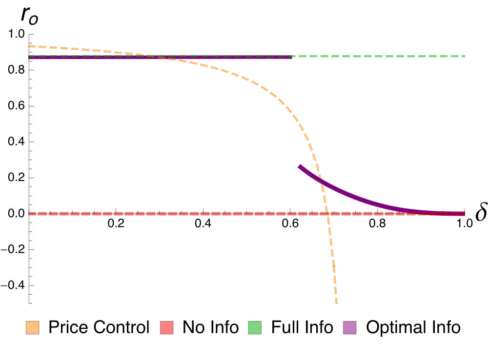
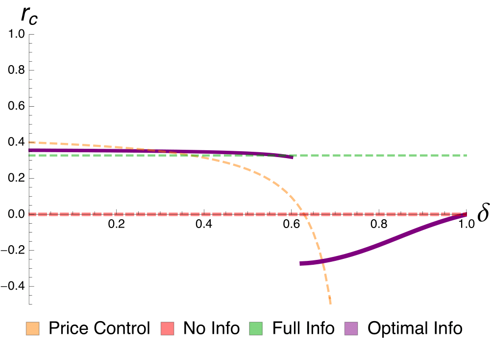
Figure 1: Price responsiveness to own demand shock (left) and opponent’s demand shock (right) under price control, no information, full information, and optimal information structure. Calculated at $c=1$, $\bar{\omega}=3$, $\sigma^{2}=1$, and $\eta=1/2$ for different values of consumer weight $\delta$.

Figure 1 reveals the presence of two distinct optimal information regimes: the coordination regime that benefits firms and the anti-coordination regime that benefits consumers. For $\delta<\hat{\delta}=11/18$, the optimally induced prices resemble those under full information, yet full information is not exactly optimal. At $\delta=0$, to benefit firms, the designer induces larger responses to the opponent’s demand. As $\delta$ increases, the price responsiveness decreases. Around $\delta=\hat{\delta}$, the optimal information structure undertakes a discontinuous structural change: $r_{o}$ plummets in absolute value, whereas $r_{c}$ changes its sign, so firms begin responding oppositely to the same demand shock. As $\delta$ further increases in the region $\delta>\hat{\delta}$, the responsiveness parameters gradually decrease in their absolute values. At $\delta=1$, both parameters equal zero; a designer who wishes to maximize solely consumer surplus should not inform firms at all.

Why does the optimal information structure exhibit discontinuous change with respect to the consumer weight? Formally, the linear certificate evaluated at $(x^{*},y^{*})$ changes continuously for all $\delta\in(0,1)$. However, at $\delta=\hat{\delta}$, the certificate permits a range of the dual agent’s best responses that connect one branch of best responses to another, so that the implemented allocation rule displays a jump. Intuitively, the pricing induced under the optimal information structure aims to approximate its first-best counterpart under direct price control. However, without the ability to enforce prices directly, the designer opts for one of the two information regimes that better approximates it.

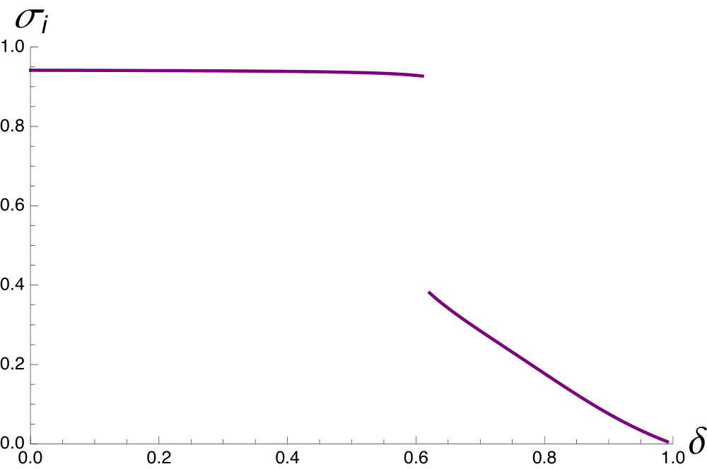
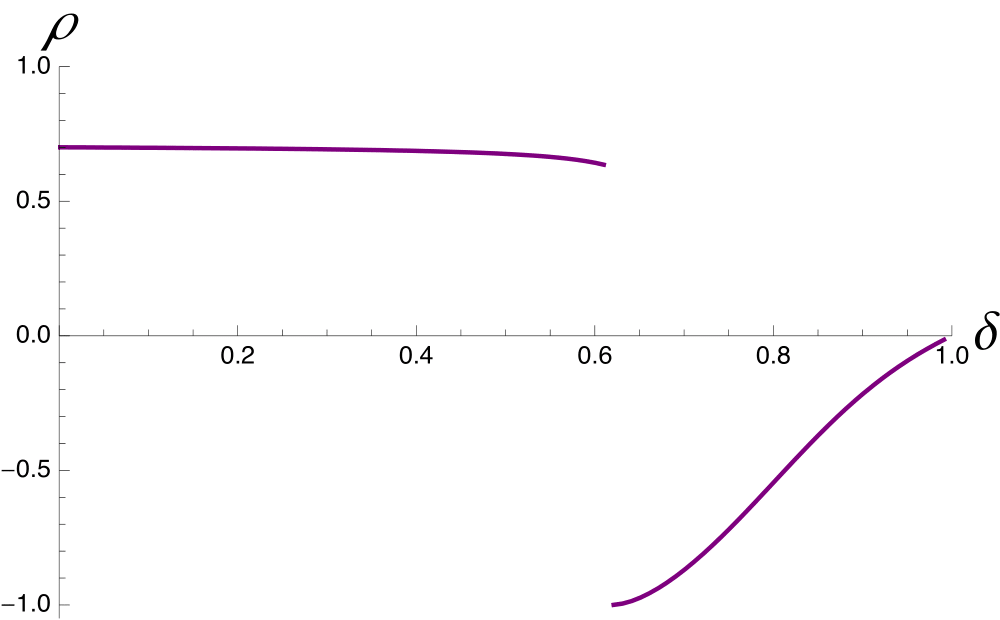
Figure 2: Optimal price volatility (left) and price correlation (right). Calculated at $c=1$, $\bar{\omega}=3$, $\sigma^{2}=1$, and $\eta=1/2$ for different values of consumer weight $\delta$.

The two optimal information regimes translate into distinct patterns of price volatility and correlation, that can be measured as the standard deviation and the Pearson correlation coefficient respectively (Figure 2):

$$\sigma_{i} =\textrm{var}(a_{i})^{1/2}=\sigma(r_{o}^{2}+r_{c}^{2})^{1/2},$$ (43)

$$\rho =\frac{\textrm{cov}(a_{i},a_{-i})}{\sigma_{i}\sigma_{-i}}=\frac{2r_{o}r_{c}}{r_{o}^{2}+r_{c}^{2}}.$$ (44)

For lower consumer weights, the price volatility is high, and the prices are positively correlated. This region is marked by coordination and high volatility of prices. In contrast, for higher consumer weights, the price volatility is low, and the product prices are negatively correlated. This region is associated with anticoordination and low volatility of prices.

5 Discussion

5.1 On Certifiably Optimal Information Structures

Robustness

An allocation rule induced by a certifiably optimal information structure must be undertaken at will by a dual agent in possession of full information. This observation has two consequences. First, the prior state distribution is irrelevant for the implementability of an allocation rule by incentives since the prescribed action profiles must be optimal state-by-state. Second, if the optimal allocation rule randomizes over several action profiles at some state, the dual agent must be indifferent between these profiles and hence could just as well randomize over these profiles with different probabilities. As a result, only the action support is relevant for implementability by incentives. Consequently, by Theorem 1, we have the following result.

Proposition 6.

(Robustness) Let two concave information-design problems differ only in their prior state distributions, if at all. Let $\pi_{1}\in\Delta(A\times\Omega)$ be certifiably optimal in the first problem. If $\pi_{2}\in\Delta(A\times\Omega)$ is implementable by information in the second problem and $\textup{supp}\,\pi_{2}(\cdot\mid\omega)\subseteq\textup{supp}\,\pi_{1}(\cdot\mid\omega)$ for all $\omega\in\Omega$, then $\pi_{2}$ is certifiably optimal in the second problem.

6 demonstrates a certain robustness of certifiably optimal information structures, i.e., once optimal under some prior distribution, an information structure remains optimal under other prior distributions if it continues to implement an allocation rule with the same or smaller support in each state. This property generalizes the robustness to prior distribution of targeted disclosure that we observed in Section 4.1. It is specific to our setting that features a continuum of actions and thus more flexible players’ best-responses. In contrast, in generic games with finitely many actions, a given allocation rule is implementable for many prior distributions, yet the optimal allocation rule continuously changes with the prior.

6 enables us to assess the optimality of full state transparency. We say that an information structure is fully informative about the state if each player deduces the state with certainty, i.e., each private signal induces an extreme posterior belief about the state. There could be many such structures, each differing in the state-by-state coordination of players’ actions. However, any such structure implements the same allocation rule under all prior state distributions. Therefore, it remains certifiably optimal.

Corollary 2.

(Full State Information) If a certifiably optimal information structure is fully informative about the state, then it is certifiably optimal under all prior state distributions.

6 highlights the importance of the support of equilibrium action profiles under certifiably optimal information structures. Generally, the larger the support is, the easier it is to construct multiple information structures that implement allocation rules within that support. In the extreme case, if the action support covers the whole action space, then the support condition of 6 has no bite, and any information structure can be certified to be optimal.

Corollary 3.

(Full-Support Noise) If measure $\pi\in\Delta(A\times\Omega)$ is certifiably optimal and $\textup{supp}\,\pi(\cdot\mid\omega)=A$ for all $\omega\in\Omega$, then any information structure is certifiably optimal.

3 presents a case against using extraneous noises that induce full-support action profiles in concave games with finitely many players. The information structures that employ such noises can never be certifiably optimal, except in trivial cases in which the designer’s expected payoff is invariant to the information provided. This finding resonates with the analysis of Taneva (2019), who studied a binary setting with two players and showed that sending conditionally independent signals is never strictly optimal, and with the analysis of Candogan and Strack (2023) who established optimality of partitional signals in a class of games. However, such extraneous independent noises may optimally appear in the limit information structure as the number of players grows to infinity, as we discuss in Section 5.3.

Multiplicity

The applications presented in Section 4.1 and Section 4.2 demonstrate the potential for multiple optimal information structures. For concreteness, consider the persuasion of investors from Section 4.1. First, within the class of targeted disclosure, an informed player can be chosen at will. Second, if the state follows a normal distribution, it is easy to show that there exist symmetric Gaussian information structures that implement the same total investment function and are thus certifiably optimal. This multiplicity is substantive: different optimal information structures implement different allocation rules and yield different players’ payoffs.

One way to explain this multiplicity is to note that in those applications different optimal information structures induce the same aggregate action behavior, and in large-scale games, with multiple receivers and a continuum of actions and states, there are many ways to implement the same aggregate behavior. This observation resonates with the research on robust information design in regime change games, such as Inostroza and Pavan (2023) and Morris, Oyama, and Takahashi (2023), which is fundamentally concerned with multiple informational implementations of the same aggregate behavior.

5.2 On the Scope of Certification Approach

Can any optimal information structure be certified? By the arguments leading to Theorem 1, the difference $V^{D}-V^{P}$ between the optimal values of primal and dual problems is nonnegative and constitutes a duality gap. The solution to the information-design problem can be certified if and only if (i) solutions to both primal and dual problems exist, and (ii) the duality gap is equal to zero, $V^{D}=V^{P}$. Thus, either all optimal information structures can be certified or none of them can (cf. 1).

While proving properties (i) and (ii) from the first principles and in full generality is challenging in our setting, it is important to emphasize that Theorem 1 does not require any additional qualifications. Any constructed certificate, by its very existence, proves that the duality gap is zero, and both primal and dual solutions exist. As in our applications in Section 4, we expect the certification approach to be useful and tractable in a variety of economic settings.

5.3 Extensions

Bounded Action Spaces

We have assumed that action spaces are unbounded, to avoid corner solutions and simplify the exposition. However, the certification approach can be easily extended to games with upper and lower bounds on each player’s action space, as demonstrated in Appendix B. The primal problem formulation remains the same, except that the boundary first-order conditions must be inequalities rather than equalities. The dual problem formulation is identical, with the added sign constraints on the contract functions evaluated at the boundary actions.

Infinite Economies

Our analysis considers games with a finite number of players. It does not directly cover games with a continuum of players, as considered in the literature on quadratic infinite economies, e.g., by Angeletos and Pavan (2007) and Bergemann and Morris (2013), even though we anticipate that an analogous certification approach, suitably extended, would work in those settings as well.

However, our analysis enables determining an optimal information structure in a game with a fixed number of players and then examining its limit as the number of players approaches infinity. We hypothesize that in many quadratic economies with a normally distributed state, Gaussian information structures are certifiably optimal and an optimal aggregate behavior is a deterministic function of a state. With a finite number of players, the latter condition necessitates the designer to either not introduce extraneous noise at all or to ensure that the noises are carefully correlated. With an infinite number of players, this condition can be met by adding independent noises and relying on the law of large numbers; the optimal aggregate behavior can be ensured by the large population size rather than by noise correlation. At the same time, our analysis suggests that even in infinite economies, alternative information structures such as targeted disclosure may also be optimal, and robustly so.

General Smooth Games

The tractability of the certification approach in concave games hinges on the capacity of first-order conditions to succinctly represent players’ incentives. In general smooth games, these first-order conditions might be not sufficient as they may select a suboptimal local maximum or a minimum in player’s payoff. However, they remain necessary, which enables a straightforward extension of our analysis: in a smooth but not necessarily concave information-design problem, one constructs a relaxed primal problem that features only first-order conditions. This problem can be solved using the certification approach. In the final step, one verifies whether players obey the recommendation of the information structure found. If so, this information structure solves the original information-design problem.

6 Conclusion

In this paper, we have outlined a certification approach for solving information-design problems in games. We have shown the effectiveness and tractability of this approach in classic economic environments. Our findings shed light on disclosure practices that guide investment, on the socially efficient control of information in markets, and on the limits of Bayesian polarization. Along the way, we have provided justification for the use of targeted disclosure and Gaussian information structures.

Our analysis lays the groundwork and offers tools for studying information design in general smooth games with multiple players. We see at least two promising avenues for further research. First, our theoretical framework can be applied to study other novel economic settings, including contests, public good provision, as well as labor and financial markets. Second, the theoretical framework can be expanded to include elements like information elicitation, information spillovers across players, and dynamic interaction. We expect all of these developments be feasible based on the approach we have outlined.

Appendix A Appendix

A.1 Formalism Omitted in Section 2

Derivation of First-Order Condition (4)

For $\varepsilon>0$, define

$$\phi_{i\varepsilon}^{+}(a_{i},a_{-i},\omega) \triangleq\frac{u_{i}(a_{i}+\varepsilon,a_{-i},\omega)-u_{i}(a_{i},a_{-i},\omega)}{\varepsilon},$$

$$\phi_{i\varepsilon}^{-}(a_{i},a_{-i},\omega) \triangleq\frac{u_{i}(a_{i},a_{-i},\omega)-u_{i}(a_{i}-\varepsilon,a_{-i},\omega)}{\varepsilon}.$$

Definition 3.

(Admissible Equilibria) An equilibrium is admissible, if for any player $i$ and equilibrium belief $\mu_{i}\in\Delta(A_{-i}\times\Omega)$, there exist a best response $a_{i}^{*}\in A_{i}$, $\Delta>0$, and $\psi:A_{-i}\times\Omega\to\mathbb{R}$ such that $\int_{A_{-i}\times\Omega}\psi(a_{-i},\omega)d\mu_{i}<+\infty$ and for all $\varepsilon\in(0,\Delta)$, $(a_{-i},\omega)\in A_{-i}\times\Omega$, $|\phi_{i\varepsilon}^{+}(a_{i}^{*},a_{-i},\omega)|\leq\psi(a_{-i},\omega)$ and $|\phi_{i\varepsilon}^{-}(a_{i}^{*},a_{-i},\omega)|\leq\psi(a_{-i},\omega)$ .

The admissibility effectively requires that players’ payoff differences are locally well behaved at best responses. It ensures the interchangeability of operators in (4) and is satisfied in all equilibria that we characterize. (If $A$ and $\Omega$ were compact, then admissibility would be trivially satisfied whenever each ${u}_{i}(a,\omega)$ is continuously differentiable in $a_{i}$.)

Lemma 2.

(First-Order Approach) Under 1, for any player $i$ and admissible equilibrium belief $\mu_{i}\in\Delta(A_{-i}\times\Omega)$, $a_{i}$ is player $i$’s best response if and only if condition (4) is satisfied.

Proof.

For any $i$ and admissible equilibrium belief $\mu_{i}$, $a_{i}^{*}$ satisfies the following condition:

$$\int_{A_{-i}\times\Omega}u_{i}(a_{i}^{*},a_{-i},\omega)\textrm{d}\mu_{i}\geq\int_{A_{-i}\times\Omega}u_{i}(a_{i},a_{-i},\omega)\textrm{d}\mu_{i},\quad\forall a_{i}\in A_{i}.$$ (45)

Under 1, condition (45) is satisfied if and only if for any $\varepsilon>0$, the following holds:

$$\int_{A_{-i}\times\Omega}\phi_{i\varepsilon}^{+}(a_{i}^{*},a_{-i},\omega)\textrm{d}\mu_{i}\leq 0,$$ (46)

$$\int_{A_{-i}\times\Omega}\phi_{i\varepsilon}^{-}(a_{i}^{*},a_{-i},\omega)\textrm{d}\mu_{i}\geq 0.$$ (47)

Moreover, $\phi_{i\varepsilon}^{+}$ is decreasing in $\varepsilon$ and $\phi_{i\varepsilon}^{-}$ is increasing in $\varepsilon$, so conditions (46), (47) are equivalent to

$$0\geq\lim_{\varepsilon\rightarrow 0}\int_{A_{-i}\times\Omega}\phi_{i\varepsilon}^{+}(a_{i}^{*},a_{-i},\omega)\textrm{d}\mu_{i} =\lim_{\varepsilon\rightarrow 0}\frac{1}{\varepsilon}\int_{A_{-i}\times\Omega}u_{i}(a_{i}^{*}+\varepsilon,a_{-i},\omega)-u_{i}(a_{i}^{*},a_{-i},\omega)\ \textrm{d}\mu_{i}$$

$$=\left.\frac{\partial^{+}}{\partial a_{i}}\int_{A_{-i}\times\Omega}u_{i}(a_{i},a_{-i},\omega)\textrm{d}\mu_{i}\right|_{a_{i}=a_{i}^{*}},$$

$$0\leq\lim_{\varepsilon\rightarrow 0}\int_{A_{-i}\times\Omega}\phi_{i\varepsilon}^{-}(a_{i}^{*},a_{-i},\omega)\textrm{d}\mu_{i} =\lim_{\varepsilon\rightarrow 0}\frac{1}{\varepsilon}\int_{A_{-i}\times\Omega}u_{i}(a_{i}^{*},a_{-i},\omega)-u_{i}(a_{i}^{*}-\varepsilon,a_{-i},\omega)\ \textrm{d}\mu_{i},$$

$$=\left.\frac{\partial^{-}}{\partial a_{i}}\int_{A_{-i}\times\Omega}u_{i}(a_{i},a_{-i},\omega)\textrm{d}\mu_{i}\right|_{a_{i}=a_{i}^{*}}.$$

By Lebesgue’s dominated convergence theorem (Theorem 11.32, Rudin (1976)), because belief $\mu_{i}$ arises in an admissible equilibrium, the following holds:

$$\lim_{\varepsilon\rightarrow 0}\int_{A_{-i}\times\Omega}\phi_{i\varepsilon}^{+}(a_{i}^{*},a_{-i},\omega)\textrm{d}\mu_{i} =\int_{A_{-i}\times\Omega}\lim_{\varepsilon\rightarrow 0}\phi_{i\varepsilon}^{+}(a_{i}^{*},a_{-i},\omega)\textrm{d}\mu_{i}=\int_{A_{-i}\times\Omega}\dot{u}_{i}(a_{i}^{*},a_{-i},\omega)\textrm{d}\mu_{i},$$

$$\lim_{\varepsilon\rightarrow 0}\int_{A_{-i}\times\Omega}\phi_{i\varepsilon}^{-}(a_{i}^{*},a_{-i},\omega)\textrm{d}\mu_{i} =\int_{A_{-i}\times\Omega}\lim_{\varepsilon\rightarrow 0}\phi_{i\varepsilon}^{-}(a_{i}^{*},a_{-i},\omega)\textrm{d}\mu_{i}=\int_{A_{-i}\times\Omega}\dot{u}_{i}(a_{i}^{*},a_{-i},\omega)\textrm{d}\mu_{i},$$

and thus

$$\left.\frac{\partial}{\partial a_{i}}\int_{A_{-i}\times\Omega}u_{i}(a_{i},a_{-i},\omega)\textrm{d}\mu_{i}\right|_{a_{i}=a_{i}^{*}}=\int_{A_{-i}\times\Omega}\dot{u}_{i}(a_{i}^{*},a_{-i},\omega)\textrm{d}\mu_{i}=0.$$

∎

A.2 Formalism Omitted in Section 3

Proof of Theorem 1

The first step is:

Lemma 3.

(Weak Duality) $V^{P}\leq V^{D}.$

Proof.

Take any dual variables $(\lambda,\gamma)$ that satisfy the constraints of the dual problem (9). Take any measure $\pi$ that satisfies the constraints of the primal problem (6). Integrating both sides of the dual constraints over $a\in A$ and $\omega\in\Omega$ against measure $\pi$ yields:

$$\int_{A\times\Omega}v(a,\omega)\textrm{d}\pi \leq\int_{A\times\Omega}\sum_{i=1}^{N}\lambda_{i}(a_{i})\dot{u}_{i}(a,\omega)\textrm{d}\pi+\int_{A\times\Omega}\gamma(\omega)\textrm{d}\pi=\int_{\Omega}\gamma(\omega)\textrm{d}\mu_{0},$$ (48)

where the equality follows because $\pi$ satisfies the primal constraints. The left-hand side of (48) is the value of the primal problem given measure $\pi$. The right-hand side of (48) is the value of the dual problem given dual variables $(\lambda,\gamma)$. As the inequality (48) holds for any allowed values of primal measure and dual variables, it also holds at the respective maximization and minimization limits. ∎

Continuing with the proof of Theorem 1, take any primal measure $\pi$ implementable by information, i.e., that satisfies the constraints of the primal problem (6). If it is implementable by incentives, then there exist dual variables $\lambda$ that implement this measure in the dual problem (11), and

$$V^{D} =\inf_{\lambda^{\prime}\in\times_{i}\mathscr{M}(A_{i})}\mathbb{E}_{\mu_{0}}\left[\sup_{a\in A}w(a,\omega,\lambda^{\prime})\right]$$

$$\leq\mathbb{E}_{\pi}\left[w(a,\omega,\lambda)\right]$$

$$=\int_{A\times\Omega}v(a,\omega)\textrm{d}\pi-\int_{A\times\Omega}\sum_{i=1}^{N}\lambda_{i}(a_{i})\dot{u}_{i}(a,\omega)\textrm{d}\pi$$

$$=\int_{A\times\Omega}v(a,\omega)\textrm{d}\pi\leq V^{P},$$

where the first inequality follows from the implementability of $\pi$ in the dual problem and the last three steps follow from the feasibility of $\pi$ in the primal problem.

Furthermore, by 3, $V^{D}\geq V^{P}$. Combining the two inequalities, we obtain

$$V^{D}=\int_{A\times\Omega}v(a,\omega)\textrm{d}\pi=V^{P},$$

which proves the optimality of measure $\pi$.

Proof of 1

For any optimal measure $\pi$, the following holds:

$$\mathbb{E}_{\pi}[v(a,\omega)]=V^{P},$$

$$\int_{A^{\prime}_{i}\times A_{-i}\times\Omega}\dot{u}_{i}(a,\omega)\textrm{d}\pi=0\quad\forall\,i=1,\dots,N,\textrm{measurable\ }A^{\prime}_{i}\subseteq A_{i}.$$

As such, if the dual agent is offered contract $\lambda$ and plays according to an optimal measure then his expected payoff is

$$\mathbb{E}_{\pi}[w(a,\omega,\lambda)] =\mathbb{E}_{\pi}[v(a,\omega)-\sum_{i=1}^{N}\lambda_{i}(a_{i})\dot{u}_{i}(a,\omega)]$$

$$=\mathbb{E}_{\pi}[v(a,\omega)]-\mathbb{E}_{\pi}[\sum_{i=1}^{N}\lambda_{i}(a_{i})\dot{u}_{i}(a,\omega)]=V^{P}.$$

That is, the dual agent obtains the same expected payoff of $V^{P}$ by playing according to an optimal measure, be it $\pi$ or $\pi^{\prime}$, irrespective of a contract.

At the same time, if $\lambda$ certifies the optimality of measure $\pi$, then playing according to $\pi$ is a best response of the dual agent to contract $\lambda$. However, since, as we showed above, $\pi^{\prime}$ delivers the same expected dual payoff as $\pi$, it follows that $\pi^{\prime}$ is also a best response of the dual agent to contract $\lambda$.

Finally, as an optimal measure, $\pi^{\prime}$ satisfies the constraints of the primal problem. Hence, $\pi^{\prime}$ is implementable by information and by incentives and, by definition, $\lambda$ certifies the optimality of $\pi^{\prime}$.

A.3 Formalism Omitted in Section 4.1

No Information

Under no information, each player’s action cannot depend on the state and is thus uniquely determined by condition (17).

Full Information

For any $\omega$, the ensuing game admits a strictly concave potential $\Psi(a,\omega)=(\omega-\frac{A}{2})A-\sum_{i=1}^{N}a_{i}^{2}$ and thus has a unique equilibrium. Parameterize a symmetric linear strategy profile:

$$a_{i}(\omega)=k_{0}+k_{1}\omega.$$

The best-response condition (15) can be rewritten as

$$a_{i}(\omega)=-\frac{N-1}{2}k_{0}+\frac{1-k_{1}(N-1)}{2}\omega,$$

which pins down the equilibrium parameters at $k_{0}=0$ and $k_{1}=\frac{1}{N+1}$.

Proof of 2

In the main text, we derived the allocation rule implemented by targeted disclosure. By Theorem 1, it is left to show that the allocation rule can be implemented by incentives. The dual payoff is

$$w(a,\omega) =v(a,\omega)-\sum_{i=1}^{N}\lambda_{i}(a_{i})\dot{u}_{i}(a,\omega)=(\omega-\overline{a})\overline{a}-\sum_{i=1}^{N}\lambda_{i}(a_{i})r(\omega-\overline{a}-a_{i}).$$

Set the contract to be $\lambda(a_{i})=\frac{N-1}{r(N+1)^{2}}\mathbb{E}[\omega]$. The dual payoff can be rewritten as

$$w(a,\omega) =(\omega-\overline{a})\overline{a}-\frac{N-1}{(N+1)^{2}}\mathbb{E}[\omega](N(\omega-\overline{a})-A).$$

For any $\omega$, the payoff is concave and quadratic in $\overline{a}$ with a unique maximizer satisfying

$$\overline{a}(\omega)=\frac{1}{2}\left(\omega+\frac{N-1}{N+1}\mathbb{E}[\omega]\right),$$

which corresponds to (23). As such, any allocation rule that results in this $\overline{a}(\omega)$ is implementable by incentives, including the one implemented by targeted disclosure.

A.4 Formalism Omitted in Section 4.3

We can microfound the linear demand as being generated by a continuum of consumers that differ in their tastes. Each consumer has a type $\omega=(\omega_{1},\omega_{2})\in\mathbb{R}^{2}$ and decides how much of the firms’ products to consume, $q=(q_{1},q_{2})$. The payoff of a type-$\omega$ consumer who consumes quantities $q$ at prices $a$ is:

$$-a^{T}q+\frac{1}{2}(\omega-q)^{T}H^{-1}(\omega-q),$$

where $H$ is an $N\times N$ negative semidefinite matrix

$$H\triangleq\left(\begin{array}[]{cc}-1&\eta\\ \eta&-1\end{array}\right).$$

For any price vector $a\in A$, the quantities demanded by a type-$\omega$ consumer are $q(a,\omega)=\omega+Ha$.

Consumer and producer surpluses can be written as:

$$CS(a,\omega) =a^{T}B_{CS}\omega-\frac{1}{2}a^{T}C_{CS}a,$$

$$PS(a,\omega) =a^{T}(\omega+Ha)-c(\omega+Ha)^{T}(\omega+Ha)=-c\omega^{T}\omega+a^{T}B_{PS}\omega-\frac{1}{2}a^{T}C_{PS}a,$$

where the payoff coefficient matrices are:

$$B_{CS}\triangleq-I,\ C_{CS}\triangleq H,$$

$$B_{PS}\triangleq I-2cH,\ C_{PS}\triangleq-2H+2cH^{2},$$

$$B\triangleq\delta B_{CS}+(1-\delta)B_{PS},\ C\triangleq\delta C_{CS}+(1-\delta)C_{PS}.$$

Price Control

The designer’s first-order condition is

$$B\omega-Ca=0,$$

which results in the first-best responsiveness matrix $R^{FB}=C^{-1}B.$ The threshold value $\overline{\delta}$ is the one that equalizes the determinant of $C$ to zero:

$$\overline{\delta}=\frac{2+2c(1-|\eta|)}{3+2c(1-|\eta|)}.$$

Benchmark Information

Equilibrium pricing behavior can be derived from the system of first-order conditions:

$$\mathbb{E}_{\mu}[q_{i}(a_{i},a_{-i},\omega)+\frac{\partial q_{i}(a_{i},a_{-i},\omega)}{\partial a_{i}}(a_{i}-2ca_{i})]=0,\quad i=1,2.$$

Substituting the linear form (27) of demand function $q_{i}$ and setting belief $\mu$ equal to $\mu_{0}$ for no-information equilibrium, we obtain:

$$a^{NI}_{i}=\frac{1+2c}{2(1+c)-\eta(1+2c)}\bar{\omega}.$$

Analogously, by setting the belief concentrated on $\omega$ for full-information equilibrium, we obtain:

$$a^{FI}_{i}(\omega)=r_{o}^{FI}\omega_{i}+r_{c}^{FI}\omega_{-i}=\frac{2(1+c)(1+2c)}{4(1+c)^{2}-\eta^{2}(1+2c)^{2}}\omega_{i}+\frac{\eta(1+2c)^{2}}{4(1+c)^{2}-\eta^{2}(1+2c)^{2}}\omega_{-i}.$$

Proof of 5

To simplify the exposition, and to provide greater generality, we parameterize the payoffs by $p_{o},p_{c},q_{o},q_{c}$ and $\tilde{p}_{o},\tilde{p}_{c},\tilde{q}_{o},\tilde{q}_{c}$ as

$$u_{i}(a,\omega)=p_{o}\omega_{i}a_{i}+p_{c}\omega_{-i}a_{i}+\frac{q_{o}}{2}a_{i}^{2}+q_{c}a_{i}a_{-i}+\textrm{term}(a_{-i},\omega),$$

$$v(a,\omega)=\tilde{p}_{o}(\omega_{1}a_{1}+\omega_{2}a_{2})+\tilde{p}_{c}(\omega_{1}a_{2}+\omega_{2}a_{1})+\tilde{q}_{o}(a_{1}^{2}+a_{2}^{2})+2\tilde{q}_{c}a_{1}a_{2},$$

where the coefficients satisfy the following conditions: $p_{o}>0$, $q_{o}<0$, and $|q_{c}|<|q_{o}|$, so that $q_{o}-q_{c}<0$ and $q_{o}+q_{c}<0$. In our application, these coefficients are as follows:

$$p_{o} =1+2c, \tilde{p}_{o} =\delta(-1)+(1-\delta)(1+2c),$$ (49)

$$p_{c} =0, \tilde{p}_{c} =\delta*0+(1-\delta)(-2c\eta),$$ (50)

$$q_{o} =-2(1+c), \tilde{q}_{o} =\delta*\frac{1}{2}+(1-\delta)(-1-c(1+\eta^{2})),$$ (51)

$$q_{c} =\eta(1+2c), \tilde{q}_{c} =\delta(-\frac{1}{2}\eta)+(1-\delta)\eta(1+2c),$$ (52)

so we set $p_{c}=0$ for the rest of this section. For a given linear contract $\lambda_{i}(a_{i};x,y)$ the dual payoff is

$$w(a,\omega,\lambda)=v(a,\omega)+\sum_{i=1}^{2}(xa_{i}+y)(p_{o}\omega_{i}+q_{o}a_{i}+q_{c}a_{-i}).$$

This payoff is quadratic in $a=(a_{1},a_{2})$ with the non-linear term being $a^{T}\mathrm{M}(x)a$, where

$$\mathrm{M}(x)\triangleq\left(\begin{array}[]{cc}\tilde{q}_{o}+xq_{o}&\tilde{q}_{c}+xq_{c}\\ \tilde{q}_{c}+xq_{c}&\tilde{q}_{o}+xq_{o}\end{array}\right)=\left(\begin{array}[]{cc}\overline{q}_{o}(x)&\overline{q}_{c}(x)\\ \overline{q}_{c}(x)&\overline{q}_{o}(x)\end{array}\right)$$

and $\overline{q}_{o}(x)\triangleq\tilde{q}_{o}+xq_{o}$, $\overline{q}_{c}(x)\triangleq\tilde{q}_{c}+xq_{c}$, $\overline{p}_{o}(x)\triangleq\tilde{p}_{o}+xp_{o}$, $\overline{p}_{c}\triangleq\tilde{p}_{c}+x*p_{c}=\tilde{p}_{c}$. For the sake of readability, we will omit the dependence of $\overline{q}_{o}$, $\overline{q}_{c}$, $\overline{p}_{o}$ and $\overline{p}_{c}$ on $x$ for the rest of this section.

The following lemma is elementary:

Lemma 4.

$\mathrm{M}$(x) is negative definite if and only if

$$x>\underline{x}\triangleq\max\left\{-\frac{\tilde{q}_{o}-\tilde{q}_{c}}{q_{o}-q_{c}},-\frac{\tilde{q}_{o}+\tilde{q}_{c}}{q_{o}+q_{c}}\right\}.$$ (53)

For $x<\underline{x}$, the expected dual payoff diverges. For $x>\underline{x}$, it holds that $\overline{q}_{o}<0$, $\overline{q}_{o}^{2}-\overline{q}_{c}^{2}>0$, $\overline{q}_{o}+\overline{q}_{c}<0$, and the dual agent’s best response exists, unique and equals to

$$\hat{a}_{i}(\omega;x,y)=-\frac{1}{2(\overline{q}_{o}^{2}-\overline{q}_{c}^{2})}\left((q_{o}+q_{c})(\overline{q}_{o}-\overline{q}_{c})y+(\overline{q}_{o}\overline{p}_{o}-\overline{q}_{c}\overline{p}_{c})\omega_{i}+(\overline{q}_{o}\overline{p}_{c}-\overline{q}_{c}\overline{p}_{o})\omega_{-i})\right).$$ (54)

The resulting expected dual payoff is

$$W(x,y)=-\frac{((q_{o}+q_{c})y+\bar{\omega}(\overline{p}_{o}+\overline{p}_{c}))^{2}-4\bar{\omega}p_{o}(\overline{q}_{o}+\overline{q}_{c})y}{2(\overline{q}_{o}+\overline{q}_{c})}-\frac{\sigma^{2}(\overline{q}_{o}\overline{p}_{o}^{2}+\overline{q}_{o}\overline{p}_{c}^{2}-2\overline{q}_{c}\overline{p}_{o}\overline{p}_{c})}{2(\overline{q}_{o}^{2}-\overline{q}_{c}^{2})}.$$

For $x>\underline{x}$, $W(x,y)$ is a differentiable function, and we aim to show that it reaches zero derivatives at some finite value. (By Theorem 1, this value would be a global minimum.) For any fixed $x$, $W(x,y)$ is a convex and quadratic function of $y$, achieving its minimum at

$$y^{*}(x)=\bar{\omega}\frac{2p_{o}(\overline{q}_{o}+\overline{q}_{c})-(\overline{p}_{o}+\overline{p}_{c})(q_{o}+q_{c})}{(q_{o}+q_{c})^{2}}.$$ (55)

The resulting expected dual payoff is

$$W(x,y^{*}(x))=-\frac{2\bar{\omega}^{2}p_{o}(p_{o}(\tilde{q}_{o}+\tilde{q}_{c})-(\tilde{p}_{o}+\tilde{p}_{c})(q_{o}+q_{c}))}{(q_{o}+q_{c})^{2}}-\frac{\sigma^{2}(\overline{q}_{o}\overline{p}_{o}^{2}+\overline{q}_{o}\overline{p}_{c}^{2}-2\overline{q}_{c}\overline{p}_{o}\overline{p}_{c})}{2(\overline{q}_{o}^{2}-\overline{q}_{c}^{2})}.$$ (56)

It remains to show that $W(x,y^{*}(x))$ diverges to $+\infty$ as $x\downarrow\underline{x}$ and $x\uparrow+\infty$.

Lemma 5.

(Divergence at Extremes) If neither of the conditions (i), (ii), (iii) is satisfied, then $W(x,y^{*}(x))$ diverges to $+\infty$ as $x\downarrow\underline{x}$ or $x\uparrow+\infty$. The conditions are as follows:
(i) $(q_{o}-q_{c})(\tilde{p}_{o}-\tilde{p}_{c})=(\tilde{q}_{o}-\tilde{q}_{c})p_{o}$ and $(q_{o}+q_{c})(\tilde{q}_{o}-\tilde{q}_{c})\leq(\tilde{q}_{o}+\tilde{q}_{c})(q_{o}-q_{c})$,
(ii) $(q_{o}+q_{c})(\tilde{p}_{o}+\tilde{p}_{c})=(\tilde{q}_{o}+\tilde{q}_{c})p_{o}$ and $(q_{o}+q_{c})(\tilde{q}_{o}-\tilde{q}_{c})\geq(\tilde{q}_{o}+\tilde{q}_{c})(q_{o}-q_{c})$,
(iii) $q_{c}\tilde{q}_{o}-\tilde{q}_{c}q_{o}=0$ and $\tilde{p}_{c}^{2}q_{o}^{2}+2\tilde{p}_{c}q_{c}(p_{o}\tilde{q}_{o}-\tilde{p}_{o}q_{o})+(\tilde{p}_{o}q_{o}-p_{o}\tilde{q}_{o})^{2}=0.$

Proof.

The first term of (56) is independent of $x$. For the second term, there are three cases to consider:
1.) $x\downarrow\underline{x}$ and $(q_{o}+q_{c})(\tilde{q}_{o}-\tilde{q}_{c})\leq(\tilde{q}_{o}+\tilde{q}_{c})(q_{o}-q_{c})$. In this case, $\underline{x}=-\frac{\tilde{q}_{o}-\tilde{q}_{c}}{q_{o}-q_{c}}\geq-\frac{\tilde{q}_{o}+\tilde{q}_{c}}{q_{o}+q_{c}}$, and

$$\sigma^{2}(\overline{q}_{o}\overline{p}_{o}^{2}+\overline{q}_{o}\overline{p}_{c}^{2}-2\overline{q}_{c}\overline{p}_{o}\overline{p}_{c}) \rightarrow_{x\downarrow\underline{x}}\ \sigma^{2}\frac{((q_{o}-q_{c})(\tilde{p}_{o}-\tilde{p}_{c})-(\tilde{q}_{o}-\tilde{q}_{c})p_{o})^{2}(q_{c}\tilde{q}_{o}-\tilde{q}_{c}q_{o})}{(q_{c}-q_{o})^{3}}$$

$$\qquad+\frac{\tilde{p}_{c}^{2}q_{o}^{2}+2\tilde{p}_{c}q_{c}(p_{o}\tilde{q}_{o}-\tilde{p}_{o}q_{o})+(\tilde{p}_{o}q_{o}-p_{o}\tilde{q}_{o})^{2}}{q_{o}}(x-\underline{x})+o((x-\underline{x})^{2})$$

$$2(\overline{q}_{o}^{2}-\overline{q}_{c}^{2}) \rightarrow_{x\downarrow\underline{x}}\ -4(q_{c}\tilde{q}_{o}-\tilde{q}_{c}q_{o})(x-\underline{x})+o((x-\underline{x})^{2}).$$

Hence, as long as conditions (i) and (iii) are not satisfied, $W(x,y^{*}(x))$ diverges to $+\infty$.
2.) $x\downarrow\underline{x}$ and $(q_{o}+q_{c})(\tilde{q}_{o}-\tilde{q}_{c})\geq(\tilde{q}_{o}+\tilde{q}_{c})(q_{o}-q_{c})$. In this case, $\underline{x}=-\frac{\tilde{q}_{o}+\tilde{q}_{c}}{q_{o}+q_{c}}\geq-\frac{\tilde{q}_{o}-\tilde{q}_{c}}{q_{o}-q_{c}}$, and

$$\sigma^{2}(\overline{q}_{o}\overline{p}_{o}^{2}+\overline{q}_{o}\overline{p}_{c}^{2}-2\overline{q}_{c}\overline{p}_{o}\overline{p}_{c}) \rightarrow_{x\downarrow\underline{x}}\ \sigma^{2}\frac{((q_{o}+q_{c})(\tilde{p}_{o}+\tilde{p}_{c})-(\tilde{q}_{o}+\tilde{q}_{c})p_{o})^{2}(q_{c}\tilde{q}_{o}-\tilde{q}_{c}q_{o})}{(q_{c}-q_{o})^{3}}$$

$$\qquad+\frac{\tilde{p}_{c}^{2}q_{o}^{2}+2\tilde{p}_{c}q_{c}(p_{o}\tilde{q}_{o}-\tilde{p}_{o}q_{o})+(\tilde{p}_{o}q_{o}-p_{o}\tilde{q}_{o})^{2}}{q_{o}}(x-\underline{x})+o((x-\underline{x})^{2})$$

$$2(\overline{q}_{o}^{2}-\overline{q}_{c}^{2}) \rightarrow_{x\downarrow\underline{x}}\ -4(q_{c}\tilde{q}_{o}-\tilde{q}_{c}q_{o})(x-\underline{x})+o((x-\underline{x})^{2}).$$

Hence, as long as conditions (ii) and (iii) are not satisfied, $W(x,y^{*}(x))$ diverges to $+\infty$.
3.) $x\uparrow+\infty$. In this case, $(\overline{q}_{o}^{2}-\overline{q}_{c}^{2})/x^{2}\rightarrow(q_{o}^{2}-q_{c}^{2})>0$, whereas $(\overline{q}_{o}\overline{p}_{o}^{2}+\overline{q}_{o}\overline{p}_{c}^{2}-2\overline{q}_{c}\overline{p}_{o}\overline{p}_{c})/x^{3}\rightarrow q_{o}p_{o}^{2}<0$. Therefore, $W(x,y^{*}(x))\rightarrow+\infty$. ∎

Consequently, as long as neither condition of Lemma 5 is satisfied, $W(x,y)$ attains a minimum at some finite value where its partial derivatives are zero.

In our application, with the coefficients (49–52), this requirement reduces to:

$$\delta\neq\hat{\delta}(\eta,c)\triangleq\frac{2+6c+4c^{2}-8c|\eta|-8c^{2}|\eta|+2c\eta^{2}+4c^{2}\eta^{2}}{5+8c+4c^{2}-|\eta|-10c|\eta|-8c^{2}|\eta|+2c\eta^{2}+4c^{2}\eta^{2}}.$$ (57)

If $\eta<0$, at $\delta=\hat{\delta}$ condition (i) holds. If $\eta>0$, at $\delta=\hat{\delta}$ condition (ii) holds. If $\eta=0$, at $\delta=\hat{\delta}$ condition (iii) holds. Otherwise, the conditions (i), (ii), and (iii) do not hold.

The remaining steps of the proof follow as presented in the main text. Whenever $\delta\neq\hat{\delta}$, the optimal direct information structure is unique and is given by (54) with $x^{*}>\underline{x}$ being a minimizer of (56) and $y^{*}$ being given by (55). The induced actions are linear in the states, which concludes the proof.

Numerical Example

At $c=1$, $\eta=1/2$, by condition (57) $\hat{\delta}=11/18$, and by condition (53)

$$\underline{x}=\max\left\{\frac{18\delta-15}{22},\frac{4\delta-3}{10}\right\}.$$

Given that $\bar{\omega}=3$ and $\sigma^{2}=1$, the expected dual payoff, as defined in (56) can be expressed as

$$W(x,y^{*}(x))=\frac{2}{25(45+72\delta^{2}+216x+220x^{2}-2\delta(57+134x))}\left(-12015+31717\delta^{3}-57902x\right.$$

$$\left.-57015x^{2}+3600x^{3}-\delta^{2}(69463+119098x)+\delta(50278+167872x+95745x^{2})\right).$$

The value of $x$ that minimizes $W(x,y^{*}(x))$ satisfies the following equation:

$$(2996\delta^{4}-7880\delta^{3}+ 7490\delta^{2}-3000\delta+414)+(6728\delta^{3}-20948\delta^{2}+20234\delta-6210)x$$

$$+(-52780\delta^{2}+88084\delta-36368)x^{2}+(77184\delta-62208)x^{3}-31680x^{4}=0.$$ (58)

Equation (58) can be solved in radicals for any $\delta\in[0,1]$. A solution $x^{*}$ greater than $\underline{x}$ corresponds to a linear certificate $\lambda_{i}(a_{i};x^{*},y^{*}(x^{*}))$ and direct information structure (54), where $y^{*}(x^{*})$ is given by (55). Numerical calculations show that such an $x$ is unique for all $\delta\neq\hat{\delta}$ and its value is continuous in $\delta$. The numerical values derived from these calculations were used to create the figures presented in the main text.

Appendix B Bounded Action Spaces

Consider the concave information-design problem as in the main text, but let the action space of each player be $A_{i}=[\underline{a}_{i},\overline{a}_{i}]$, $-\infty<\underline{a}_{i}<\overline{a}_{i}<+\infty$. For any given $\mu\in\Delta(A_{-i}\times\Omega)$, the player’s best-response action $a_{i}^{*}(\mu)$, if interior, must be unimprovable by local deviations to lower and higher actions and hence satisfies the first-order condition

$$\mathbb{E}_{\mu}\left[\dot{u}_{i}(a_{i}^{*},a_{-i},\omega)\right]=0.$$

In contrast, the optimal boundary actions must only be unimprovable by one-sided local deviations. As such, the player’s best response if located on the boundary must satisfy the following:

$$\mathbb{E}_{\mu}\left[\dot{u}_{i}(\underline{a}_{i}^{*},a_{-i},\omega)\right]\leq 0,$$ (59)

$$\mathbb{E}_{\mu}\left[\dot{u}_{i}(\overline{a}_{i}^{*},a_{-i},\omega)\right]\geq 0.$$ (60)

We can write the resulting primal information-design problem as follows:

$$V^{P}_{B}\triangleq\sup_{\pi\in\Delta(A\times\Omega)} \int_{A\times\Omega}v(a,\omega)\textrm{d}\pi$$ (61)

s.t. $$\int_{A^{\prime}_{i}\times A_{-i}\times\Omega}\dot{u}_{i}(a,\omega)\textrm{d}\pi=0\quad\forall\,i=1,\dots,N,\textrm{measurable\ }A^{\prime}_{i}\subseteq(\underline{a}_{i},\overline{a}_{i}),$$ (62)

$$\int_{A^{\prime}_{i}\times A_{-i}\times\Omega}\dot{u}_{i}(a,\omega)\textrm{d}\pi\leq 0\quad\forall\,i=1,\dots,N,\textrm{measurable\ }A^{\prime}_{i}\subseteq[\underline{a}_{i},\overline{a}_{i}),$$ (63)

$$\int_{A^{\prime}_{i}\times A_{-i}\times\Omega}\dot{u}_{i}(a,\omega)\textrm{d}\pi\geq 0\quad\forall\,i=1,\dots,N,\textrm{measurable\ }A^{\prime}_{i}\subseteq(\underline{a}_{i},\overline{a}_{i}],$$ (64)

$$\int_{A\times\Omega^{\prime}}\textrm{d}\pi=\int_{\Omega^{\prime}}\textrm{d}\mu_{0}\quad\forall\,\textrm{measurable\ }\Omega^{\prime}\subseteq\Omega.$$ (65)

This primal problem entails the standard dual problem

$$V^{D}_{B}\triangleq\inf_{\lambda\in\times_{i}\mathscr{M}(A_{i}),\gamma\in\mathscr{M}(\Omega)} \ \int_{\Omega}\gamma(\omega)\textrm{d}\mu_{0}$$ (66)

$$\textrm{s.t.}\ \sum_{i=1}^{N} \lambda_{i}(a_{i})\dot{u}_{i}(a,\omega)+\gamma(\omega)\geq v(a,\omega)\ \forall\,a\in A,\omega\in\Omega,$$ (67)

$$\lambda_{i}(\underline{a}_{i})\leq 0,\ \lambda_{i}(\overline{a}_{i})\geq 0\quad\forall\,i=1,\dots,N.$$ (68)

The presence of additional obedience constraints (63), (64) in the primal problem translates into the sign constraints on the Lagrange multipliers (68) in the dual problem. As in the case of unbounded actions, the dual problem (66) can be simplified and rewritten as

$$V^{D}_{B}= \inf_{\lambda\in\times_{i}\mathscr{M}(A_{i})}\mathbb{E}_{\mu_{0}}[\sup_{a\in A}w(a,\omega,\lambda)]$$ (69)

s.t. $$\lambda_{i}(\underline{a}_{i})\leq 0,\ \lambda_{i}(\overline{a}_{i})\geq 0\quad\forall\,i=1,\dots,N.$$ (70)

The adversarial-contracting interpretation remains intact, but the space of allowed contracts is limited at the boundary actions by the presence of sign constraints.

Lemma 6.

(Weak Duality with Bounded Action Spaces) $V^{P}_{B}\leq V^{D}_{B}.$

Proof.

Take any dual variables $(\lambda,\gamma)$ that satisfy the constraints of the dual problem (66). Take any measure $\pi$ that satisfies the constraints of primal problem (61). Integrating both sides of the dual constraints over $a\in A$ and $\omega\in\Omega$ against measure $\pi$ yields:

$$\int_{A\times\Omega}v(a,\omega)\textrm{d}\pi \leq\int_{A\times\Omega}\sum_{i=1}^{N}\lambda_{i}(a_{i})\dot{u}_{i}(a,\omega)\textrm{d}\pi+\int_{A\times\Omega}\gamma(\omega)\textrm{d}\pi\leq\int_{\Omega}\gamma(\omega)\textrm{d}\mu_{0},$$ (71)

where the second inequality follows because $\pi$ satisfies the primal constraints and the Lagrange multipliers satisfy the dual constraints. (This inequality holds as equality in the case of unbounded actions.) The left-hand side of (71) is the value of the primal problem given measure $\pi$. At the same time, the right-hand side of (71) is the value of the dual problem given dual variables $(\lambda,\gamma)$. As inequality (71) holds for any allowed values of primal measure and dual variables, it also holds at the respective maximization and minimization limits. ∎

In the case of bounded actions, we say that the measure $\pi\in\Delta(A\times\Omega)$ is implementable by information if it satisfies the constraints of the primal problem (61) and that it is implementable by incentives if there exists a feasible contract in the dual problem (69) that induces this measure as a best response.

Theorem 2.

(Optimality Certification with Bounded Action Spaces) In the case of bounded actions, if $\pi\in\Delta(A\times\Omega)$ is implementable by information and is implementable by incentives by contract $\lambda$, then (i) $\pi$ solves the information-design problem, (ii) $\lambda$ solves the adversarial-contracting problem, and (iii) $V^{P}=V^{D}$.

Proof.

Take any primal measure $\pi$ implementable by information, i.e., that satisfies the constraints of the primal problem (61). If it is implementable by incentives, then there exist dual variables $\lambda$ that implement this measure in the dual problem (69), and

$$V^{D}_{B} =\inf_{\lambda^{\prime}\in\times_{i}\mathscr{M}(A_{i})}\mathbb{E}_{\mu_{0}}\left[\sup_{a\in A}w(a,\omega,\lambda^{\prime})\right]$$

$$\leq\mathbb{E}_{\pi}\left[w(a,\omega,\lambda)\right]$$

$$=\int_{A\times\Omega}v(a,\omega)\textrm{d}\pi-\int_{A\times\Omega}\sum_{i=1}^{N}\lambda_{i}(a_{i})\dot{u}_{i}(a,\omega)\textrm{d}\pi$$

$$\leq\int_{A\times\Omega}v(a,\omega)\textrm{d}\pi\leq V^{P}_{B},$$

where the first inequality follows from the implementability of $\pi$ in the dual problem and the last three steps follow from the feasibility of $\pi$ in the primal problem and the sign constraints on dual variables. (The next-to-last step holds as equality in the case of unbounded actions.)

Furthermore, by 6, $V^{D}_{B}\geq V^{P}_{B}$. Hence,

$$V^{D}_{B}=\int_{A\times\Omega}v(a,\omega)\textrm{d}\pi=V^{P}_{B},$$

which proves the optimality of measure $\pi$. ∎

References

- Amador and Bagwell (2013) Amador, M. and K. Bagwell (2013): “The Theory of Optimal Delegation with an Application to Tariff Caps,” Econometrica, 81, 1541–1599.
- Amador et al. (2006) Amador, M., I. Werning, and G.-M. Angeletos (2006): “Commitment vs. Flexibility,” Econometrica, 74, 365–396.
- Anderson and Nash (1987) Anderson, E. and P. Nash (1987): Linear Programming in Infinite-dimensional Spaces: Theory and Applications, Wiley.
- Angeletos and Pavan (2007) Angeletos, G.-M. and A. Pavan (2007): “Efficient Use of Information and Social Value of Information,” Econometrica, 75, 1103–1142.
- Angeletos and Pavan (2009) ——— (2009): “Policy with Dispersed Information,” Journal of the European Economic Association, 7, 11–60.
- Arieli and Babichenko (2019) Arieli, I. and Y. Babichenko (2019): “Private Bayesian Persuasion,” Journal of Economic Theory, 182, 185–217.
- Arieli and Babichenko (2022) ——— (2022): “A Population’s Feasible Posterior Beliefs,” Working paper.
- Arieli et al. (2023) Arieli, I., Y. Babichenko, and F. Sandomirskiy (2023): “Persuasion as Transportation,” Working paper.
- Arieli et al. (2021) Arieli, I., Y. Babichenko, F. Sandomirskiy, and O. Tamuz (2021): “Feasible Joint Posterior Beliefs,” Journal of Political Economy, 129, 2546–2594.
- Bergemann et al. (2015) Bergemann, D., T. Heumann, and S. Morris (2015): “Information and Volatility,” Journal of Economic Theory, 158, 427–465.
- Bergemann et al. (2017) ——— (2017): “Information and Interaction,” Working paper.
- Bergemann et al. (2021) ——— (2021): “Information, Market Power, and Price Volatility,” RAND Journal of Economics, 52, 125–150.
- Bergemann and Morris (2013) Bergemann, D. and S. Morris (2013): “Robust Predictions in Games with Incomplete Information,” Econometrica, 81, 1251–1308.
- Bergemann and Morris (2016) ——— (2016): “Bayes Correlated Equilibrium and the Comparison of Information Structures in Games,” Theoretical Economics, 11, 487–522.
- Bergemann and Morris (2019) ——— (2019): “Information Design: A Unified Perspective,” Journal of Economic Literature, 57, 44–95.
- Brooks and Du (2021) Brooks, B. and S. Du (2021): “Optimal Auction Design with Common Values: An Informationally Robust Approach,” Econometrica, 89, 1313–1360.
- Candogan and Strack (2023) Candogan, O. and P. Strack (2023): “Optimal Disclosure of Information to Privately Informed Agents,” Theoretical Economics, 18, 1225–1269.
- Carroll (2017) Carroll, G. (2017): “Robustness and Separation in Multidimensional Screening,” Econometrica, 85, 453–488.
- Chan et al. (2019) Chan, J., S. Gupta, F. Li, and Y. Wang (2019): “Pivotal Persuasion,” Journal of Economic theory, 180, 178–202.
- Chiappori et al. (2017) Chiappori, P.-A., B. Salanié, and Y. Weiss (2017): “Partner Choice, Investment in Children, and the Marital College Premium,” American Economic Review, 107, 2109–2167.
- Dizdar and Kováč (2020) Dizdar, D. and E. Kováč (2020): “A Simple Proof of Strong Duality in the Linear Persuasion Problem,” Games and Economic Behavior, 122, 407–412.
- Du (2018) Du, S. (2018): “Robust Mechanisms under Common Valuation,” Econometrica, 86, 1569–1588.
- Dworczak and Kolotilin (2022) Dworczak, P. and A. Kolotilin (2022): “The Persuasion Duality,” Working paper.
- Dworczak and Martini (2019) Dworczak, P. and G. Martini (2019): “The Simple Economics of Optimal Persuasion,” Journal of Political Economy, 127, 1993–2048.
- Elliott et al. (2022) Elliott, M., A. Galeotti, A. Koh, and W. Li (2022): “Market Segmentation through Information,” Working paper.
- Galichon and Salanié (2022) Galichon, A. and B. Salanié (2022): “Cupid’s Invisible hand: Social Surplus and Identification in Matching Models,” Review of Economic Studies, 89, 2600–2629.
- Galperti et al. (2023) Galperti, S., A. Levkun, and J. Perego (2023): “The Value of Data Records,” Review of Economic Studies, rdad044.