Choquet-Based Fuzzy Rough Sets
Abstract
Fuzzy rough set theory can be used as a tool for dealing with inconsistent data when there is a gradual notion of indiscernibility between objects. It does this by providing lower and upper approximations of concepts. In classical fuzzy rough sets, the lower and upper approximations are determined using the minimum and maximum operators, respectively. This is undesirable for machine learning applications, since it makes these approximations sensitive to outlying samples. To mitigate this problem, ordered weighted average (OWA) based fuzzy rough sets were introduced. In this paper, we show how the OWA-based approach can be interpreted intuitively in terms of vague quantification, and then generalize it to Choquet-based fuzzy rough sets (CFRS). This generalization maintains desirable theoretical properties, such as duality and monotonicity. Furthermore, it provides more flexibility for machine learning applications. In particular, we show that it enables the seamless integration of outlier detection algorithms, to enhance the robustness of machine learning algorithms based on fuzzy rough sets.
keywords:
Fuzzy rough sets , Non-additive measures , Choquet integral , Machine learning , Outlier detection1 Introduction
Rough set theory, introduced by Pawlak [1], provides a lower and upper approximation of a concept with respect to the indiscernibility relation between objects. The lower and upper approximation contain all objects that are certainly, resp. possibly part of the concept. That is to say, an element is a member of the lower approximation of a concept if every element indiscernible from it belongs to the concept; and an element is a member of the upper approximation of the concept if there exists an element indiscernible from it that belongs to the concept. Rough set theory was first extended to fuzzy rough set theory by Dubois and Prade [2], here both the concept and the indiscernibility relation can be fuzzy. Fuzzy rough set theory has been used successfully for classification and other machine learning purposes, such as feature and instance selection [3], but due to the fact that the approximations in classical fuzzy rough sets are determined using the minimum and maximum operators, these approximations (and the applications based on them) are sensitive to noisy and outlying samples. To mitigate this problem, many noise-tolerant versions of fuzzy rough sets (FRS) have been proposed, such as Vaguely Quantified FRS [4], -Precision FRS [5, 6], Variable Precision FRS [7], Variable Precision -FRS [8], Soft Fuzzy Rough Sets [9], Automatic Noisy Sample Detection FRS [10], Data-Distribution-Aware FRS [11], Probability Granular Distance based FRS [12] and Ordered Weighted Averaging (OWA) based FRS [13].
The Choquet integral, which is commonly used in decision making [14], is a generalization of the Lebesgue integral to non-additive measures. It induces an interesting class of aggregation operators, that contains the weighted mean and OWA operators as special cases.
In this paper, we introduce a generalization of OWA-based fuzzy rough sets (OWAFRS), called Choquet-based fuzzy rough sets (CFRS), that uses the Choquet integral to determine the lower and upper approximation of a concept. This adds extra flexibility for machine learning purposes, while still retaining the important theoretical properties that OWAFRS has, such as monotonicity w.r.t. the indiscernibility relation and duality. We also show how OWAFRS can be interpreted in terms of vague quantification. Furthermore, we explain and demonstrate how to combine CFRS and normalized outlier scores [15] to boost the robustness of the lower and upper approximations in fuzzy rough sets.
This paper is structured as follows: in Section 2, we recall the required prerequisites for (OWA-based) fuzzy rough sets and Choquet integration, while Section 3 discusses vague quantification. Section 4 combines the previous sections to link OWAFRS with vague quantification and introduces CFRS together with several non-symmetric monotone measures that can be used with CFRS. These measures have a concrete interpretation in terms of vague quantification and let us smoothly combine outlier detection algorithms and fuzzy rough sets, moreover they cannot be realised using the OWAFRS approach. In Section 5, these measures are applied and evaluated for classification. Section 6 concludes this paper and describes opportunities for future research.
2 Preliminaries
2.1 Fuzzy set theory
In this subsection, we recall the necessary notions of fuzzy set and fuzzy logical connectives. We start with the definition of a fuzzy set and a fuzzy relation.
Definition 2.1.
[16] A fuzzy set or membership function on is a function from to the unit interval, i.e. . The value of an element is called the degree of membership of in the fuzzy set . The set of all fuzzy sets on is denoted as . A fuzzy relation on is an element of .
Definition 2.2.
[16] The notation for two fuzzy sets and , expresses that for all . The fuzzy set is defined by .
We will also make use of conjunctors, implicators and negators which extend their Boolean counterparts to the fuzzy setting.
Definition 2.3.
-
•
A function is called a conjunctor if it is increasing in both arguments and satisfies , and for all . A commutative and associative conjunctor is called a t-norm.
-
•
A function is called an implicator if , and for all in the following holds:
-
1.
(decreasing in the first argument),
-
2.
(increasing in the second argument),
-
1.
-
•
A function is called a negator if it is non-increasing and satisfies and .
-
•
The induced conjunctor of an implicator and negator is defined by:
Since t-norms are required to be associative, they can be extended naturally to a function for any natural number .
Example 2.4.
-
•
The minimum and product operators are t-norms: and .
-
•
The Kleene-Dienes, Reichenbach and Łukasiewicz implicators are defined by , and .
-
•
The standard negator is defined by for .
-
•
The induced conjunctor of the Kleene-Dienes implicator and the standard negator is the minimum t-norm.
Definition 2.5.
Given a negator , the -complement of a fuzzy set is given by:
2.2 Fuzzy rough sets
Rough sets, first introduced by Pawlak [1], try to model uncertainty that is associated with indiscernibility. Here indiscernibility is defined with respect to an equivalence relation, and two elements are called indiscernible if they are in the same equivalence class. Indiscernibility arises naturally in information systems.
Definition 2.6.
An information system , consists of a finite non-empty set and a non-empty family of attributes , where each attribute is a function , with the set of values the attribute can take. A decision system is an information system , where is called the decision attribute and each is called a conditional attribute.
Definition 2.7 (-indiscernibility).
Let be a subset of , then the -indiscernibility relation is given by
If then and are said to be indiscernible with respect to . The equivalence class of is denoted by .
Definition 2.8.
[1] Let be a subset of and an equivalence relation on . The lower and upper approximations of with respect to are defined as:
where denotes the equivalence class of with respect to . The pair is called a rough set.
If an element is in the lower approximation of , then we know that all elements that are indiscernible from are also in . When an element is in the upper approximation of , we can only say that there exists some element that is indiscernible from and belongs to .
For fuzzy sets and fuzzy relations, the lower and upper approximations can be extended as follows:
Definition 2.9.
[17] Given and , the lower and upper approximation of w.r.t. are defined as:
| (1) | ||||
| (2) |
where is an implicator and a conjunctor.
2.3 OWA-based fuzzy rough sets
A downside to the classical definition of lower and upper approximation in fuzzy rough set theory is their lack of robustness. The value of the membership of an element in the lower and upper approximation is fully determined by a single element because of the minimum and maximum operators in the definition. To solve this undesirable behaviour, OWA-based fuzzy rough sets were introduced in [13]. The Ordered Weighted Average [18] is an aggregation operator that is defined as follows:
Definition 2.10 (OWA operator).
Let , and be a weighting vector, i.e. , then the ordered weighted average of with respect to is defined as
where is a permutation of such that
Example 2.11.
The maximum, mean and minimum operators can all be seen as OWA-operators with weight vectors , and respectively.
In OWA-based fuzzy rough sets, OWA operators replace the minimum and maximum in equations (1) and (2). To not deviate too strongly from the original definitions, some requirements may be enforced on the weight vectors of the OWA-operators used [13]. In particular, we require that the OWA-operator for the lower approximation is a soft minimum and for the upper approximation a soft maximum.
Definition 2.12.
The orness and andness of a weight vector are defined as
| (3) | ||||
If , then is called a soft minimum. If , is called a soft maximum.
As can be seen from Equation (3), the orness indicates how much weight is given to the largest elements. The orness tells us how “close” the OWA-operator is to the maximum. Using this definition OWA-based fuzzy rough sets are then defined as:
Definition 2.13.
[13] Given , weight vectors and with and and , the OWA lower and upper approximation of w.r.t. , and are given by:
| (4) | ||||
| (5) |
where is an implicator, a conjunctor and and are seen as functions in .
2.4 The Choquet integral
The Choquet integral induces a large class of aggregation functions, namely the class of all comonotone linear aggregation functions [19]. Since we will view the Choquet integral as an aggregation operator, we will restrict ourselves to measures (and Choquet integrals) on finite sets. For the general setting, we refer the reader to e.g. [20].
Definition 2.14.
A function is called a monotone measure if:
-
•
and
-
•
A monotone measure is called:
-
•
additive if when and are disjoint
-
•
symmetric if when
Definition 2.15.
[20] Let be a monotone measure on and a real-valued function. The Choquet integral of with respect to the measure is defined as:
where is a permutation of such that
and .
The following proposition gives an equivalent definition of the Choquet integral:
Proposition 2.16.
Corollary 2.17.
[20] The following equality holds for every monotone measure , constant and real-valued function :
The class of aggregation operators induced by the Choquet integral contains the weighted mean and the OWA operator. In fact, the weighted mean and OWA operator are the Choquet integrals with respect to additive and symmetric measures, respectively.
Proposition 2.18.
[19] The Choquet integral with respect to an additive measure is the weighted mean with weight vector . Conversely, the weighted mean , with weight vector is a Choquet integral with respect to the uniquely defined additive measure for which .
Proposition 2.19.
[19] The Choquet integral with respect to a symmetric measure is the OWA operator with weight vector , where denotes any subset with cardinality . Conversely, the OWA operator with weight vector is a Choquet integral with respect to the symmetric measure defined as
Lastly we recall the definition of a dual measure and take a look at how this concept translates to the case of OWA operators.
Definition 2.20.
[20] The dual measure of a monotone measure is defined by:
Proposition 2.21.
[20] Let be a monotone measure on and a real-valued function on . Then
Proposition 2.22.
If is the symmetric measure corresponding to the OWA operator with weights , then corresponds to the OWA operator with weights .
3 Vague quantification
In this section, we recall the models of Zadeh [21] and Yager [22] for vague quantification and we show how particular fuzzy quantifiers correspond to symmetric measures. Vague quantification models linguistic quantifiers such as “most”, “some”, “almost all”, etc.
3.1 Zadeh’s model of vague quantification
Zadeh’s model represents a proportional linguistic quantifier as a fuzzy set of the unit interval. If is the proportion for which a certain proposition holds, then determines the truth value of the quantified proposition.
Definition 3.23.
[21] A fuzzy set is called a regular increasing monotone (RIM) quantifier if is a non-decreasing function such that and .
Example 3.24.
The following RIM quantifiers represent the universal and existential quantifier:
Linguistic quantifiers such as “most” and “some” can be modelled using the RIM quantifiers () [4]:
for example, we could use and to model “most” and “some”, respectively.
Let be a RIM quantifier, Zadeh then uses to evaluate the truth value of the proposition as
where and the cardinality of a fuzzy set is interpreted using Zadeh’s -count, i.e. .
3.2 Yager’s model of vague quantification
Yager’s approach also represents quantifiers as fuzzy sets of the unit interval, but uses OWA aggregation for the evaluation of the truth values. He evaluates propositions of the form “’s are ’s”, where is a RIM quantifier and is a fuzzy set, as
| (6) |
Example 3.25.
Suppose is the set of all basketball players and the fuzzy set describing tallness. Then the truth value of the statement “most basketball players are tall”, in Yager’s model, is given by:
where Equation (6) is used with .
In Zadeh’s model this evaluates to:
Notice that the truth value in Yager’s model is closer to what one might expect, since half of the basketball players only have a membership degree of to the fuzzy set “tall people”. The reason for this is that Zadeh’s model only looks at the average membership degree, whereas Yager’s model gives weight to each instance according to its relative degree of membership.
The next definition and proposition describe the relationship between weight vectors and RIM quantifiers.
Definition 3.26.
A RIM quantifier is associated with a weight vector if interpolates the following set of points:
| (7) |
Two RIM quantifiers are called semantically equivalent (on a universe ) if they are associated with the same weight vector.
Proposition 3.27.
A RIM quantifier is associated with a weight vector if and only if
| (8) |
for every .
Proof.
Suppose is a RIM quantifier that interpolates the points
then
Conversely, suppose
for every . By induction we have that
∎
Corollary 3.28.
Semantically equivalent RIM quantifiers have the same truth value for propositions of the form “’s are ’s” (Equation (6)).
The previous proposition gives us a one-to-one correspondence (modulo RIM quantifiers with equivalent semantics) between RIM quantifiers and OWA weights, when the universe is fixed. Indeed, for every OWA weight vector , we can define as the unique step function that interpolates the set of points defined in Equation (7):
which is indeed a RIM quantifier since is a weight vector. Conversely, we have Equation (8).
Example 3.29.
A common weighting scheme (cf. [23]) for the OWA operator, in the context of fuzzy rough lower approximations, is the additive weight vector defined by
We now want to find a quantifier that is associated with . More specifically, has to interpolate the set of points
so we get, by applying the substitution , that the following RIM quantifier corresponds to :
Since we know that weight vectors of OWA operators are equivalent to symmetric measures, we can also convert a RIM quantifier into a symmetric measure (Proposition 2.19):
| (9) |
and we can rewrite the evaluation as follows:
| (10) |
which in the case that is crisp reduces to (follows from Definition 2.15). When is crisp, Yager’s and Zadeh’s models thus coincide.
4 Choquet-based fuzzy rough sets
4.1 Motivation and definition
Note that by Proposition 2.19, we can rewrite OWAFRS as follows:
| (11) | ||||
| (12) |
where and are two symmetric measures. From the previous section we know that these expressions can be interpreted as vaguely quantified propositions. For example, suppose is the measure corresponding with “most” and with “some”, then the degree of membership of an element to the lower approximation (Equation (11)) is equal to the truth value of the proposition “Most elements indiscernible to are in ”. Analogously we have that the degree of membership of an element to the upper approximation (Equation (12)) is equal to the truth value of the proposition “Some elements are indiscernible to and are in ”. This approach is thus intuitive, since it closely resembles the definition of rough sets. But why restrict ourselves to symmetric measures? If we allow non-symmetric measures, we gain more flexibility to reduce noise, as the following example shows.
Example 4.30.
Suppose we have a crisp set containing all the instances that are outliers, unreliable or inaccurate, then a useful pair of quantifiers could be “for all except (maybe) elements of ” and “there exists an element in ”. These quantifiers can be modelled by the partial minimum and maximum:
Proposition 4.31.
Let be a crisp subset of and , then
Proof.
Let be an ordering of such that the following inequalities hold:
where is the first index such that . Using the definition of the Choquet integral we get:
∎
Corollary 4.32.
Let be a crisp subset of and , then
Proof.
Using these non-symmetric measures in Equation (11) and (12), we get that the degree of membership of an element to the lower approximation is equal to the truth value of the proposition “All trustworthy elements that are indiscernible to are in ”. An analogous interpretation holds for the upper approximation.
As we will show in Subsection 4.2, it is possible to extend the approach of the previous example to fuzzy sets and quantifiers representing ”most of the trustworthy objects”. The following examples show how such fuzzy sets can be constructed in practice.
Example 4.33.
Suppose we have a decision system where is a categorical attribute. Then we can define as the normalized outlier score [15] of (obtained from a certain outlier detection algorithm) when compared to other elements of (based on the conditional attributes). An outlier score measures the degree to which a data point differs from other observations, and normalization transforms this score in such a way that it can be interpreted as a degree of outlierness.
Example 4.34.
Suppose consists of patients from several different hospitals, is the subset of patients that have a disease and is a similarity relation between patients based on a set of symptoms. Then a confidence score can be attached to each hospital based on the accuracy of the tests performed to trace the disease (and the symptoms). The membership degree of a patient of hospital to can then be defined as .
These examples motivate the definition of Choquet-based fuzzy rough sets (CFRS):
Definition 4.35.
Given , monotone measures and on and , then the Choquet lower and upper approximation of w.r.t. , and are given by:
where is an implicator and is a conjunctor.
Notice that we have discarded the orness conditions in the definition of OWA-based fuzzy rough sets. The reason for this is that these orness conditions were introduced mainly in the hope they would yield extra theoretical properties such as inclusion of the lower approximation in the upper approximation, but as we shall see in Subsection 4.3, they do not.
4.2 Examples of non-symmetric measures
As described in the previous subsection we can accommodate non-symmetry by introducing a fuzzy set in that represents the degree of inconfidence. The function could, for example, be seen as an outlier score in (Example 4.33) or it could represent the unreliability or inaccuracy of the observation (Example 4.34). We now define several non-symmetric measures using the fuzzy set .
4.2.1 Fuzzy removal
One option to use to define a non-symmetric measure is as follows:
| (13) |
where is a t-norm (e.g. minimum).
Proposition 4.36.
The function is a monotone measure.
Proof.
The monotonicity follows from the following property of t-norms:
which can be seen using induction, the neutral element property and the increasingness of t-norms. ∎
We will call this measure the fuzzy removal measure, since in the case is crisp, the Choquet integral with respect to this measure is equal to the partial minimum (Proposition 4.31) The vague quantifier interpretation of the fuzzy removal measure could thus be “for all except (maybe) elements of ”.
Example 4.37.
Let be the set of people who went to a party and the subset of people who tested positive for a certain disease. Now suppose we know that and went to the hospital for the test, while and used a home testing kit. Then a sensible choice for , which in this case represents the unreliability, could be , since and can report any result they want and the tests are less accurate. Then the evaluation of the sentence “all reliable tests from people at the party are positive” is:
it thus evaluates to the t-norm of all the unreliabilities of the elements that are not in . Thus if there was one element fully reliable () and with a negative test, then the sentence would evaluate to false, as expected.
4.2.2 Weighted ordered weighted average
Another idea for a non-symmetric measure is:
| (14) |
where is a RIM quantifier and a weight vector describing the confidence, reliability, accuracy or non-outlierness of each observation:
| (15) |
The measure in Equation (14) corresponds to the Weighted Ordered Weighted Averaging (WOWA) operator [24, 25], which is a generalization of the OWA and the weighted mean. The RIM quantifier determines the OWA part of the WOWA and the weight vector the weighted mean part. The WOWA operator is also equivalent with Yager’s importance weighted quantifier guided aggregation [22]. These measures could be interpreted as quantifiers of the form “ of the trustworthy/reliable objects”.
Example 4.38.
Recall Example 4.37, and suppose we want to evaluate the sentence “Most reliable tests from people at the party are positive”. Then a suitable choice for the measure would be Equation (14) together with Equation (15) and the RIM quantifier “most” from Example 3.24. The sentence can then be evaluated as:
If we do not take into account reliability, i.e. we evaluate the sentence “Most people at the party are tested positive” we get:
which is, as expected, smaller than when considering reliability.
Another WOWA operator that could be used goes as follows: suppose is a permutation on such that the following inequalities hold:
Using this ordering we can define a measure as:
| (16) |
where is a RIM quantifier and an -dimensional weight vector. The weight can be thought of as the weight given to the element with the th smallest membership in . If for all , we get the symmetric measure defined by (9). Suppose are all roughly zero and the rest roughly one, in other words we partitioned in a set of non-outliers and a set of outliers (or accurate and inaccurate observations etc.). Then the following weight vector could be meaningful:
| (17) |
where is the weight given to the outliers. Notice that the measure from Equation (16), together with the weights from Equation (17), can be written as follows (when is crisp):
| (18) |
The measure of a set only depends on the cardinalities and , it is thus a two-symmetric measure [26]. If then can be seen as a symmetric measure on the set . On the other hand if , then we don’t exclude outliers to any degree, and have a symmetric measure on .
4.3 Theoretical properties of CFRS
In this subsection, we take a look at the theoretical properties of CFRS. We start out with the following proposition that states that the only pair of measures for which the lower approximation is necessarily contained in the upper approximations, corresponds to the universal and existential quantifier.
Proposition 4.40.
If and are two monotone measures such that
| (19) |
holds for every equivalence relation and crisp set , then and .
Proof.
Let be a non-empty subset, , and be two monotone measures satisfying Equation 19 and the equivalence relation corresponding with the partition of . Then we have for and the constant value of the set that
since and implicators and conjunctors are extensions of their boolean counterparts. Calculating the lower and upper approximations using Definition 2.15 of the Choquet integral, we get:
Equation 19 gives us:
since this holds for an arbitrary non-empty and we have that and . ∎
Corollary 4.41.
In particular, this shows that OWAFRS does not have the inclusion property (Equation (19)), regardless of any non-trivial orness conditions.
The following propositions show that the monotonicity and duality properties are still retained by the CFRS model, it thus retains all the properties of OWAFRS that are stated in [27].
Proposition 4.42 (Relation monotonicity).
Let , and a monotone measure on , then the following holds:
Proof.
Directly follows from the decreasingness of the implicator in the first argument, the increasingness of the t-norm and the monotonicity of the Choquet integral. ∎
Proposition 4.43 (Set monotonicity).
Let , and a monotone measure on , then the following holds:
Proof.
Directly follows from the increasingness of the implicator in the second argument, the increasingness of the t-norm and the monotonicity of the Choquet integral. ∎
Proposition 4.44 (Duality).
Let be an implicator, the conjunctor induced by and the standard negator , , a monotone measure on and . Then the following holds:
Proof.
5 Application to classification
5.1 Classification using fuzzy rough sets
The goal of classification is to predict the class of an instance, given a set of examples. More specifically, the set of examples is given in the form of a decision system . For classification we assume that is a categorical attribute; the attributes of can either be categorical of numerical. The problem of classification is then to predict for a new instance , for which the evaluations of the conditional attributes are given, the value of , based on the decision system . A simple algorithm for classification [23], using fuzzy rough sets, is to classify a test instance to the decision class for which it has the greatest membership to the lower approximation of that class. To calculate these lower approximations, we need a fuzzy relation describing the similarity between instances based on the conditional attributes. When all the conditional attributes are numerical the following relation could be used:
| (20) |
where
and denotes the standard deviation of .
Let be a decision class, since is a crisp set, the membership degrees can only take values in . Using this fact, the antitonicity of an implicator in the first argument and , we can rewrite the membership of an element in the lower approximation as follows:
where is the aggregation operator corresponding to the monotone measure . Discarding the trailing one values from the previous equation, as was also done in [28], gives us the following simpler definition of the lower approximation:
which in the case of the Łukasiewicz, Kleene-Dienes and Reichenbach implicators reduces to
| (21) |
5.2 Experimental evaluation
In this subsection we evaluate the measures introduced in Subsection 4.2, when applied to classification.
5.2.1 Setup
For ease of computation, we will make use of the lower approximation defined in Equation (21), together with the indiscernibility relation from Equation (20). The aggregation operators we evaluate are:
-
•
fuzzy outlier removal, described by Equation (13), using the minimum as the t-norm (), denoted by FR,
-
•
the Choquet integral with the WOWA measure from Equation (14) using , denoted by WOWA,
- •
The baseline aggregation operators are minimum, average and OWA with and each of these three are considered with outliers (denoted by Min, Avg and OWA) and without outliers (denoted by Mino, Avgo and OWAo), resulting in different baseline operators. For we use the scores obtained from the normalised Local Outlier Factor (LOF) algorithm [15] which is implemented in the Pyod library [29]. The normalized LOF score of an instance is calculated by fitting the LOF algorithm to all the members of the class that is part of, and then using this model to calculate the LOF score of . FR and WOWA use these raw scores, while for Mino, Avgo and OWAo, the samples with the highest outlier score are labelled as outliers, where is the number of samples and the contamination parameter is set to . Except for these 9 algorithms, we will also test a combination of all of them. This combination algorithm, denoted by COMB, performs Leave-One-Out Cross-Validation (LOOCV) for each of these 9 algorithms on the training set and then chooses the best aggregation operator, evaluated using balanced accuracy
to use on the test set. When multiple aggregation operators perform equally well, it chooses one of these randomly. We evaluate the performance on 18 two-class datasets from the UCI-repository [30] by means of stratified 5-fold cross-validation. All of the datasets only have numerical features. The balanced accuracy is used as the performance measure.
| Name | # Feat. | # Inst. | IR | Name | # Feat. | # Inst. | IR |
|---|---|---|---|---|---|---|---|
| appendicitis | 7 | 106 | 4.05 | pop-failures | 18 | 540 | 10.74 |
| banknote | 4 | 1372 | 1.25 | somerville | 6 | 143 | 1.17 |
| biodeg | 41 | 1055 | 1.96 | sonar | 60 | 208 | 1.14 |
| coimbra | 9 | 116 | 1.23 | spectf | 44 | 267 | 3.85 |
| debrecen | 19 | 1151 | 1.13 | sportsarticles | 59 | 1000 | 1.74 |
| divorce | 54 | 170 | 1.02 | transfusion | 4 | 748 | 3.20 |
| haberman | 3 | 306 | 2.78 | wdbc | 30 | 569 | 1.68 |
| ilpd | 10 | 579 | 2.51 | wisconsin | 9 | 683 | 1.86 |
| ionosphere | 34 | 351 | 1.79 | wpbc | 32 | 138 | 3.93 |
5.2.2 Results and discussion
The results of the cross-validation can be seen in Table 2 together with the mean and median over all datasets. A first impression that we get from these averages and medians is that the OWA-based operators (OWA, OWAo and WOWA) outperform all the other operators. Furthermore, the results indicate that the combination of all the algorithms (COMB) performs better than the individual ones. From this we can deduce that the best aggregation operator for the training set, also performs well on the test set. For the minimum-based (Min, Mino and FR) operators we get the impression that FR performs best, and that fully removing the “outliers” (Mino) is, on average, not a good decision. This last fact could be explained by the fact that some of the datasets may not really contain “outliers”, and thus Mino is throwing away valuable information, which because of the sensitivity of the minimum to individual instances can alter the results considerably.
Table 3 displays which algorithms were used in the COMB algorithm for each dataset. The aggregation operators that were used most are Min, WOWA, and to a lesser extent FR, OWAo and TS. The rest (Mino, Avg, Avgo and OWA) were almost never used.
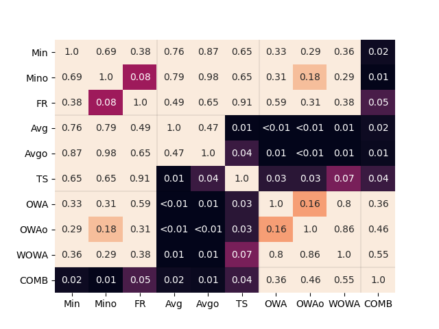
To discern if one of these methods really outperforms another method consistently and significantly we perform a two-sided Wilcoxon signed ranks test. The results of this are displayed in Figure 1. First of all we observe that COMB is significantly different from Min, Mino, FR, Avg, Avgo and TS (). From the rank sums we can tell that COMB outperforms all of them. Secondly, we notice that Avg, Avgo and TS are all significantly () different from OWA, OWAo and WOWA. Looking at the rank sums tells us that Avg, Avgo and TS perform consistently worse than the OWA-based methods. Out of all the average-based methods and TS (Avg, Avgo and TS), the Wilcoxon test indicates that TS performs the best (). For the minimum-based aggregation operators we can’t really say anything about how they compare with the other operators. What the Wilcoxon test does show is that FR consistently outperforms Mino (). From this we may conclude that when we choose to take into account “outliers”, via an outlier detection algorithm, it may be preferable to “fuzzy remove” them (FR), instead of discarding them entirely (Mino). This also suggests that even when “outliers” are present in the dataset, FR still performs better. A possible explanation for the fact that FR outperforms Mino (on average) might be that when a dataset does not contain outliers, all the outlier scores are all close to , but there still need to be outlier labels so Mino would throw away instances randomly, whereas FR would not, because it can “see” that all of the outlier scores are roughly zero.
| Dataset | Min | Mino | FR | Avg | Avgo | TS | OWA | OWAo | WOWA | COMB |
| appendicitis | 0.739 | 0.704 | 0.773 | 0.768 | 0.768 | 0.793 | 0.768 | 0.774 | 0.774 | 0.754 |
| banknote | 0.999 | 0.991 | 0.990 | 0.872 | 0.872 | 0.908 | 0.916 | 0.912 | 0.906 | 0.999 |
| biodeg | 0.817 | 0.815 | 0.820 | 0.690 | 0.707 | 0.739 | 0.753 | 0.756 | 0.763 | 0.820 |
| coimbra | 0.633 | 0.634 | 0.633 | 0.596 | 0.595 | 0.610 | 0.633 | 0.636 | 0.620 | 0.615 |
| debrecen | 0.616 | 0.619 | 0.626 | 0.576 | 0.580 | 0.616 | 0.619 | 0.622 | 0.629 | 0.630 |
| divorce | 0.976 | 0.976 | 0.976 | 0.976 | 0.976 | 0.976 | 0.976 | 0.976 | 0.976 | 0.976 |
| haberman | 0.540 | 0.581 | 0.583 | 0.625 | 0.628 | 0.602 | 0.622 | 0.634 | 0.629 | 0.634 |
| ilpd | 0.620 | 0.613 | 0.609 | 0.607 | 0.615 | 0.624 | 0.639 | 0.649 | 0.656 | 0.644 |
| ionosphere | 0.902 | 0.900 | 0.897 | 0.837 | 0.854 | 0.863 | 0.859 | 0.867 | 0.850 | 0.902 |
| pop-failures | 0.616 | 0.628 | 0.639 | 0.797 | 0.778 | 0.802 | 0.788 | 0.783 | 0.801 | 0.802 |
| somerville | 0.566 | 0.567 | 0.573 | 0.623 | 0.640 | 0.612 | 0.624 | 0.655 | 0.613 | 0.583 |
| sonar | 0.840 | 0.832 | 0.824 | 0.751 | 0.747 | 0.772 | 0.806 | 0.792 | 0.789 | 0.780 |
| spectf | 0.619 | 0.617 | 0.621 | 0.580 | 0.590 | 0.606 | 0.620 | 0.632 | 0.663 | 0.637 |
| sportsarticles | 0.729 | 0.744 | 0.745 | 0.775 | 0.775 | 0.779 | 0.782 | 0.789 | 0.783 | 0.789 |
| transfusion | 0.594 | 0.562 | 0.571 | 0.659 | 0.649 | 0.663 | 0.672 | 0.640 | 0.641 | 0.652 |
| wdbc | 0.942 | 0.943 | 0.943 | 0.911 | 0.910 | 0.915 | 0.923 | 0.927 | 0.930 | 0.943 |
| wisconsin | 0.963 | 0.958 | 0.958 | 0.894 | 0.892 | 0.922 | 0.926 | 0.926 | 0.926 | 0.967 |
| wpbc | 0.511 | 0.519 | 0.519 | 0.630 | 0.628 | 0.609 | 0.616 | 0.625 | 0.620 | 0.605 |
| Average | 0.735 | 0.733 | 0.739 | 0.731 | 0.734 | 0.745 | 0.752 | 0.755 | 0.754 | 0.763 |
| Median | 0.681 | 0.669 | 0.692 | 0.721 | 0.727 | 0.756 | 0.760 | 0.765 | 0.768 | 0.767 |
| Dataset | Min | Mino | FR | Avg | Avgo | TS | OWA | OWAo | WOWA |
| appendicitis | 0 | 0 | 1 | 1 | 0 | 0 | 0 | 1 | 2 |
| banknote | 5 | 0 | 0 | 0 | 0 | 0 | 0 | 0 | 0 |
| biodeg | 0 | 0 | 5 | 0 | 0 | 0 | 0 | 0 | 0 |
| coimbra | 0 | 0 | 0 | 0 | 0 | 3 | 0 | 0 | 2 |
| debrecen | 0 | 0 | 1 | 0 | 0 | 0 | 0 | 0 | 4 |
| divorce | 5 | 0 | 0 | 0 | 0 | 0 | 0 | 0 | 0 |
| haberman | 0 | 0 | 0 | 0 | 1 | 0 | 1 | 1 | 2 |
| ilpd | 0 | 0 | 0 | 0 | 0 | 0 | 1 | 2 | 2 |
| ionosphere | 4 | 0 | 1 | 0 | 0 | 0 | 0 | 0 | 0 |
| pop-failures | 0 | 0 | 0 | 0 | 0 | 0 | 0 | 2 | 3 |
| somerville | 0 | 0 | 1 | 1 | 1 | 0 | 0 | 1 | 1 |
| sonar | 2 | 0 | 0 | 0 | 0 | 0 | 1 | 1 | 1 |
| spectf | 1 | 0 | 0 | 0 | 0 | 0 | 0 | 0 | 4 |
| sportsarticles | 0 | 0 | 0 | 0 | 0 | 0 | 0 | 5 | 0 |
| transfusion | 0 | 0 | 0 | 1 | 0 | 3 | 0 | 0 | 1 |
| wdbc | 1 | 1 | 3 | 0 | 0 | 0 | 0 | 0 | 0 |
| wisconsin | 4 | 0 | 1 | 0 | 0 | 0 | 0 | 0 | 0 |
| wpbc | 0 | 0 | 0 | 1 | 1 | 2 | 1 | 0 | 0 |
| sum | 22 | 1 | 13 | 4 | 3 | 8 | 4 | 11 | 22 |
6 Conclusion and future work
From a theoretical perspective, Choquet-based fuzzy rough sets are a natural extension of OWA-based fuzzy rough sets as they preserve all of their known theoretical properties.
From a classification perspective, Choquet-based fuzzy rough sets yield more flexibility than OWA-based fuzzy rough sets. We have seen that they allow to combine fuzzy rough set models and outlier detection algorithms more smoothly, through fuzzy removal or weighted ordered weighted averaging. They do so by directly using the outlier scores instead of having to discretize them into outlier labels. The benefit of this is that we don’t have to optimize the contamination parameter that is used to create the outlier labels, and that this might yield a higher classification accuracy. Moreover, we have seen that choosing a good measure for a particular dataset can be done by selecting the one that performs the best on the training set.
The algorithms based on the measures introduced in this paper can still be improved, for example, by tuning the weight vector for the WOWA operator, as well by experimenting with different types of outlier detection algorithms and transformations of the outlier scores.
The measures proposed in this work are described by at most parameters, where is the length of the vector that needs to be aggregated, but an arbitrary monotone measure depends on parameters. Therefore, we still haven’t used the full generality of the Choquet integral, so one could search for measures that depend on higher dimensional characteristics of the training set, instead of the one-dimensional outlier scores.
Acknowledgment
The research reported in this paper was conducted with the financial support of the Odysseus programme of the Research Foundation – Flanders (FWO).
References
- [1] Z. Pawlak, Rough sets, International journal of computer & information sciences 11 (5) (1982) 341–356.
- [2] D. Dubois, H. Prade, Rough fuzzy sets and fuzzy rough sets, International Journal of General System 17 (2-3) (1990) 191–209.
- [3] S. Vluymans, L. D’eer, Y. Saeys, C. Cornelis, Applications of fuzzy rough set theory in machine learning: a survey, Fundamenta Informaticae 142 (1-4) (2015) 53–86.
- [4] C. Cornelis, M. De Cock, A. M. Radzikowska, Vaguely quantified rough sets, in: International Workshop on Rough Sets, Fuzzy Sets, Data Mining, and Granular-Soft Computing, Springer, 2007, pp. 87–94.
-
[5]
J. Fernández Salido, S. Murakami,
On
-precision aggregation, Fuzzy Sets and Systems 139 (3) (2003)
547–558.
doi:https://doi.org/10.1016/S0165-0114(03)00003-4.
URL https://www.sciencedirect.com/science/article/pii/S0165011403000034 -
[6]
J. Fernández Salido, S. Murakami,
Rough
set analysis of a general type of fuzzy data using transitive aggregations of
fuzzy similarity relations, Fuzzy Sets and Systems 139 (3) (2003) 635–660.
doi:https://doi.org/10.1016/S0165-0114(03)00124-6.
URL https://www.sciencedirect.com/science/article/pii/S0165011403001246 - [7] A. Mieszkowicz-Rolka, L. Rolka, Variable precision fuzzy rough sets, in: Transactions on Rough Sets I, Springer, 2004, pp. 144–160.
-
[8]
Y. Yao, J. Mi, Z. Li,
A
novel variable precision -fuzzy rough set model based on
fuzzy granules, Fuzzy Sets and Systems 236 (2014) 58–72, theme: Algebraic
Aspects of Fuzzy Sets.
doi:https://doi.org/10.1016/j.fss.2013.06.012.
URL https://www.sciencedirect.com/science/article/pii/S0165011413002753 -
[9]
Q. Hu, S. An, D. Yu,
Soft
fuzzy rough sets for robust feature evaluation and selection, Information
Sciences 180 (22) (2010) 4384–4400.
doi:https://doi.org/10.1016/j.ins.2010.07.010.
URL https://www.sciencedirect.com/science/article/pii/S0020025510003282 -
[10]
A. Hadrani, K. Guennoun, R. Saadane, M. Wahbi,
Fuzzy
rough sets: Survey and proposal of an enhanced knowledge representation model
based on automatic noisy sample detection, Cognitive Systems Research 64
(2020) 37–56.
doi:https://doi.org/10.1016/j.cogsys.2020.05.001.
URL https://www.sciencedirect.com/science/article/pii/S1389041720300255 - [11] S. An, Q. Hu, W. Pedrycz, P. Zhu, E. C. C. Tsang, Data-distribution-aware fuzzy rough set model and its application to robust classification, IEEE Transactions on Cybernetics 46 (12) (2016) 3073–3085. doi:10.1109/TCYB.2015.2496425.
-
[12]
S. An, Q. Hu, C. Wang,
Probability
granular distance-based fuzzy rough set model, Applied Soft Computing 102
(2021) 107064.
doi:https://doi.org/10.1016/j.asoc.2020.107064.
URL https://www.sciencedirect.com/science/article/pii/S1568494620310024 - [13] C. Cornelis, N. Verbiest, R. Jensen, Ordered weighted average based fuzzy rough sets, in: International Conference on Rough Sets and Knowledge Technology, Springer, 2010, pp. 78–85.
- [14] M. Grabisch, C. Labreuche, A decade of application of the Choquet and Sugeno integrals in multi-criteria decision aid, Annals of Operations Research 175 (1) (2010) 247–286.
- [15] H.-P. Kriegel, P. Kroger, E. Schubert, A. Zimek, Interpreting and unifying outlier scores, in: Proceedings of the 2011 SIAM International Conference on Data Mining, SIAM, 2011, pp. 13–24.
- [16] L. A. Zadeh, Fuzzy sets, Information and Control (1965).
- [17] A. M. Radzikowska, E. E. Kerre, A comparative study of fuzzy rough sets, Fuzzy sets and systems 126 (2) (2002) 137–155.
- [18] R. R. Yager, On ordered weighted averaging aggregation operators in multicriteria decisionmaking, IEEE Transactions on systems, Man, and Cybernetics 18 (1) (1988) 183–190.
- [19] G. Beliakov, A. Pradera, T. Calvo, et al., Aggregation functions: A guide for practitioners, Vol. 221, Springer, 2007.
- [20] Z. Wang, G. J. Klir, Generalized measure theory, Vol. 25, Springer Science & Business Media, 2010.
- [21] L. A. Zadeh, A computational approach to fuzzy quantifiers in natural languages, in: Computational linguistics, Elsevier, 1983, pp. 149–184.
- [22] R. R. Yager, Quantifier guided aggregation using owa operators, International Journal of Intelligent Systems 11 (1) (1996) 49–73.
- [23] S. Vluymans, Dealing with imbalanced and weakly labelled data in machine learning using fuzzy and rough set methods, Springer, 2019.
- [24] V. Torra, The weighted owa operator, International Journal of Intelligent Systems 12 (2) (1997) 153–166.
- [25] V. Torra, On some relationships between the wowa operator and the Choquet integral, in: Proceedings of the IPMU 1998 Conference, Paris, France, Citeseer, 1998, pp. 818–824.
- [26] P. Miranda, M. Grabisch, P. Gil, p-symmetric fuzzy measures, International Journal of Uncertainty, Fuzziness and Knowledge-Based Systems 10 (supp01) (2002) 105–123.
- [27] L. D’eer, N. Verbiest, C. Cornelis, L. Godo, A comprehensive study of implicator–conjunctor-based and noise-tolerant fuzzy rough sets: definitions, properties and robustness analysis, Fuzzy Sets and Systems 275 (2015) 1–38.
- [28] S. Vluymans, N. Mac Parthaláin, C. Cornelis, Y. Saeys, Weight selection strategies for ordered weighted average based fuzzy rough sets, Information Sciences 501 (2019) 155–171.
-
[29]
Y. Zhao, Z. Nasrullah, Z. Li,
Pyod: A Python toolbox for
scalable outlier detection, Journal of Machine Learning Research 20 (96)
(2019) 1–7.
URL http://jmlr.org/papers/v20/19-011.html -
[30]
D. Dua, C. Graff, UCI machine learning
repository (2017).
URL http://archive.ics.uci.edu/ml