GAN’SDA Wrap: Geographic And Network Structured DAta
on surfaces that Wrap around
Abstract.
There are many methods for projecting spherical maps onto the plane. Interactive versions of these projections allow the user to centre the region of interest. However, the effects of such interaction have not previously been evaluated. In a study with 120 participants we find interaction provides significantly more accurate area, direction and distance estimation in such projections. The surface of 3D sphere and torus topologies provides a continuous surface for uninterrupted network layout. But how best to project spherical network layouts to 2D screens has not been studied, nor have such spherical network projections been compared to torus projections. Using the most successful interactive sphere projections from our first study, we compare spherical, standard and toroidal layouts of networks for cluster and path following tasks with 96 participants, finding benefits for both spherical and toroidal layouts over standard network layouts in terms of accuracy for cluster understanding tasks.
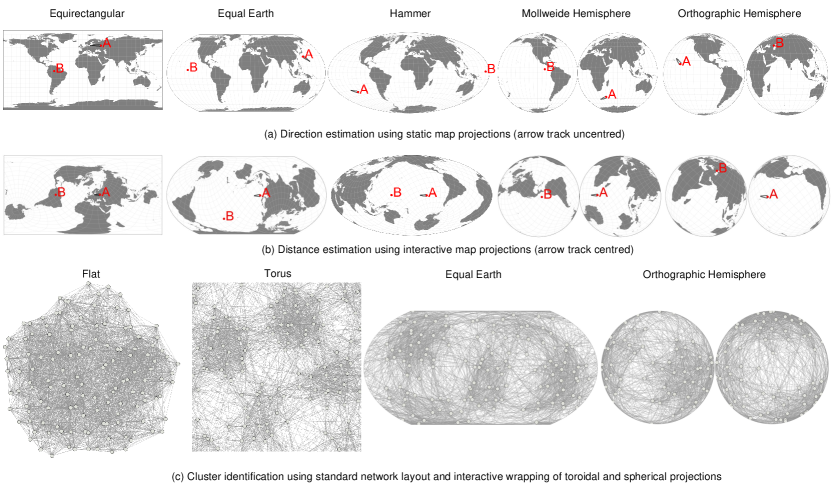
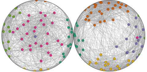
Examples of geographic and network structured data that wraps around. Top row: Direction estimation tasks of the five different spherical projections of geographic data evaluated in Study 1, with (a) and without (b) interaction. For example, for equal earth and orthographic hemisphere, the trajectory from the dot A misses dot B. Bottom row: Study 2 compares the two interactive spherical projections found most effective in Study 1, and compares them to toroidal and standard ‘flat’ layout for network data.
1. Introduction
While most people agree that the world is spherical, most computer displays remain stubbornly flat. To show maps of the entire earth’s surface on a screen we have to somehow cut, stretch and squash it. While cartographers and mathematicians have developed many methods to project the surface of a sphere to a plane, distortion or discontinuity at the edges of the projection are inevitable; with different methods achieving different trade-offs between (e.g.) area, distance, or direction preservation and discontinuities (Snyder, 1987). As a consequence distances and areas closer to the north and south poles may appear larger and the shapes more distorted than those at the centre (Jenny et al., 2017). Moreover, distances between geographical locations or areas of continents or seas that are wrapped across the projection boundary are also easily misinterpreted (Hennerdal, 2015).
Most of these projections were originally developed for static display of the earth in printed maps and atlases. However, with modern computer graphics we can create interactive versions of these projections, which can be panned, reoriented and recentred with simple mouse or touch drags (Bostock and Davies, 2013; Davies, 2013), thus allowing the viewer to centre a region of interest so as to minimise distortion and discontinuities.
But spherical projection has application beyond geographic data. There can be advantages to laying out abstract data (data which has no inherent geometry) on the surface of a sphere such that there is no arbitrary edge to the display or privileged centre (Rodighiero, 2020). In particular, node-link representations of highly connected network data (which is ubiquitous in the world around us, from protein-protein interaction networks, to social, communication, trade or electrical networks) have no real “inside” or “outside”. Arguably, they can be better distributed across the surface of a topology which “wraps around” continuously.
While the relationship between readability of geographic and network data on spherical projections has not been studied directly, there are commonalities in the analysis tasks that might be applicable for each. For example, understanding network clusters may involve comparing the relative size of their boundaries, similar to map area and shape comparison. Network path following tasks require the user to trace links (AKA ‘edges’) between nodes in the network while maps also require understanding how regions connect, and in both case splits or distortion due to spherical projection may present a challenge.
As we discuss in detail in Section 2, while there has been much work to develop the algorithms for spherical projection of maps and algorithms for layout of networks on a 3D sphere, we find that interactive 2D displays of such spherical layouts of data (whether geographic or network) are not well studied. Also projections of 3D spherical layouts of network data have not been compared to projections of networks arranged on the surface of other 3D geometries, in particular toroidal layouts which have recently been studied by Chen et al. (Chen et al., 2020, 2021a).
Therefore, this paper has two aims that are interlinked:
(1) To evaluate the effect of interaction on readability of different spherical projection techniques and identify the projection techniques which best support geographic comprehension tasks, such as distance, area and direction estimation (Study 1, Section 4).
(2) To evaluate readability of networks laid out spherically and then projected to a flat surface using the interactive techniques found most effective in Study 1, compared to conventional flat layout, and interactive projections of toroidal layout (Study 2, Section 6).
To achieve these aims many gaps in past work had to be addressed leading to seven distinct contributions:
(1) To our knowledge, we are the first to systematically evaluate the effect of introducing interactive panning on different geographic spherical projection techniques. We find that interaction overwhelmingly improves accuracy and subjective user preference compared to static projections across all projection methods and tasks considered, at the cost of increased time due to interaction (Section 4).
(2) For interactive projections, we find that the best of those tested depends on task, however, Orthographic Hemisphere
![[Uncaptioned image]](/html/2202.10845/assets/x2.png) and Equal Earth
and Equal Earth
![[Uncaptioned image]](/html/2202.10845/assets/x3.png) had advantages in terms of speed, accuracy and qualitative feedback while Equirectangular
had advantages in terms of speed, accuracy and qualitative feedback while Equirectangular
![[Uncaptioned image]](/html/2202.10845/assets/x4.png) may be a poor choice even with the ability to pan (Section 4).
may be a poor choice even with the ability to pan (Section 4).
(3) We are also the first to compare spherical network projections against toroidal and flat layouts (Section 6).
(4) We adapt a pairwise gradient descent algorithm for flat and toroidal layout (Chen et al., 2021a) to consider spherical distance between two nodes when laying them out on a 3D spherical surface. Cartographic projection to a 2D diagram results in 2D drawings whose links wrap around the edge of the display (Section 5).
(5) We present algorithms for computing how best to automatically rotate the spherical layout to minimise the number of links wrapped when projected (Section 5.2).
(6) For cluster identification tasks we find that all toroidal and spherical projections tested outperform traditional flat network layout for accuracy, while toroidal and spherical equal earth outperform orthographic projection for accuracy, speed and subjective user rank.
(7) For path following tasks we find that toroidal and traditional flat network layout outperform both spherical equal earth and orthographic hemisphere projections for accuracy and subjetive user rank (Section 6).
Our results suggest that interactive panning should be routinely provided in online maps to alleviate misconceptions arising from distortions of map projection. Our results also confirm the benefits of topologically closed surfaces, such as the surface of a torus or sphere, when using node-link diagrams to investigate network structure. This finding suggests that interactive projections of networks arranged on 3D surfaces should be more commonly used for cluster analysis tasks and further, that toroidal layouts may be a good general solution, being not only more accurate than standard flat layout for cluster tasks but also at least as accurate for path following tasks.
Collectively, we refer to the family of techniques for visualising geographic and network structured data on surfaces that wrap around by the acronym “GAN’SDA Wrap”, in a rhythmic head nod to Tupac Shakur. The full set of map and network study including training materials, instructions, study trials are available in the supplementary materials and associated OSF repository: https://osf.io/73p8w/.
2. Background
Researchers have recently investigated the utility of visualisations based on projecting the surface of a torus (Chen et al., 2020, 2021a) and a cylinder (Chen et al., 2021b) onto a flat 2D plane. These have shown benefits for understanding the structure of network diagrams (Chen et al., 2021a) and understanding cyclic time series data (Chen et al., 2021b). Crucially, these visualisations are interactive and the viewer can pan the projection so that it “wraps” around the plane. Providing interactive panning has previously been found to be of benefit in understanding network layouts based on torus projection (Chen et al., 2020). Here we investigate the utility of projections of the surface of a different geometric object, the sphere, on to a 2D plane. Again we allow the user to interactively pan the projection around the plane.
2.1. Geographical map projections
Projecting the surface of a sphere onto a 2D plane is not novel: cartographers have been doing this for centuries. Cartographers and mathematicians have devised hundreds of projection techniques (Snyder, 1997). The reason for this diversity is that none of these techniques can be considered optimal in depicting geographic information (Schöttler et al., 2021). Rather, each projection is a trade-off between preserving shape, area, distance or direction (Snyder, 1997) as it is not possible for a 2D projection to do all of these simultaneously.
As a consequence, cartographers have invented what are called equal area projections that preserve the relative area of regions on the globe. These include Equal Earth
![[Uncaptioned image]](/html/2202.10845/assets/x5.png) , Hammer
, Hammer
![[Uncaptioned image]](/html/2202.10845/assets/x6.png) and Mollweide Hemisphere
and Mollweide Hemisphere
![[Uncaptioned image]](/html/2202.10845/assets/x7.png) (see Figure 1) (Šavrič et al., 2019; Jenny et al., 2017). They have also invented compromise projections that do not preserve any of these criteria exactly but instead trade them off, creating a map that does not distort area, shape, distance or direction “too much.”
These include Orthographic Hemisphere
(see Figure 1) (Šavrič et al., 2019; Jenny et al., 2017). They have also invented compromise projections that do not preserve any of these criteria exactly but instead trade them off, creating a map that does not distort area, shape, distance or direction “too much.”
These include Orthographic Hemisphere
![[Uncaptioned image]](/html/2202.10845/assets/x8.png) and Equirectangular
and Equirectangular
![[Uncaptioned image]](/html/2202.10845/assets/x9.png) (see Figure 1).
(see Figure 1).
Projections also differ on the shape of the projection. Some, such as Equirectangular
![[Uncaptioned image]](/html/2202.10845/assets/x10.png) are rectangular, others, such as Equal Earth
are rectangular, others, such as Equal Earth
![[Uncaptioned image]](/html/2202.10845/assets/x11.png) or Hammer
or Hammer
![[Uncaptioned image]](/html/2202.10845/assets/x12.png) , reduce distortion at the poles by projecting to a more ovoid shape. Some, such as the Mollweide Hemisphere
, reduce distortion at the poles by projecting to a more ovoid shape. Some, such as the Mollweide Hemisphere
![[Uncaptioned image]](/html/2202.10845/assets/x13.png) and the Orthographic Hemisphere
and the Orthographic Hemisphere
![[Uncaptioned image]](/html/2202.10845/assets/x14.png) , resemble the front and back view
of the 3D globe. Maps such as these in which the projection region is split are said to be interrupted. The Orthographic Hemisphere
, resemble the front and back view
of the 3D globe. Maps such as these in which the projection region is split are said to be interrupted. The Orthographic Hemisphere
![[Uncaptioned image]](/html/2202.10845/assets/x15.png) , in particular, has a naturalistic appearance as it shows the Earth viewed from infinity (Jenny et al., 2017).
, in particular, has a naturalistic appearance as it shows the Earth viewed from infinity (Jenny et al., 2017).
There are several user studies on the readability and user preference of map projection visualisations, e.g. (Hennerdal, 2015; Hruby et al., 2016; Šavric et al., 2015; Carbon, 2010). In particular, these have found that viewers find it difficult to understand the distance or direction between two points if this requires reasoning about the discontinuity in the projection and mentally wrapping the projection around a globe to understand their relative position.
This suggests that allowing the viewer to interactively pan the map projection so as to centre a region of interest may improve their understanding of the inherent distortion introduced by the projection and of the Earth’s underlying geography. For instance, this allows them to reposition two points so that they are no longer separated by a discontinuity. Such interactive panning, also called spherical rotation (Snyder, 1987), has been provided in many online maps for several years, e.g. (Bostock and Davies, 2013; Davies, 2013; Jenny et al., 2016). One recent study of pannable terrain maps found that they perform more accurately than static maps but at the cost of additional time in task completion and concluded therefore that results of existing static map reading studies are likely not transferrable to interactive maps (Herman et al., 2018). However, surprisingly, as far as we are aware there has been no evaluation of whether interactive panning of globe projections improves performance on standard geographical tasks such as estimating the distance or direction between two points or the relative area of two regions.
The only direct research of pannable globes that we know of are two studies in virtual reality (VR) investigating different visualisations for understanding origin-destination flow between locations on the Earth’s surface (Yang et al., 2019). While it was not their main focus, the studies revealed that interactive panning improved task accuracy at the cost of time when viewing flow shown using straight lines on a flat map. However, it is likely that this was not because panning was used to reduce geographical distortion but rather that it was used to separate the flow lines which were the focus of the tasks. Furthermore, the static and interactive conditions were across different studies so comparison was between groups. Here we present a more systematic and direct study of interactive panning for geographic tasks.
2.2. Spherical representation of non-geographic data
Researchers have also explored non-planar geometries for visualising networks, with evidence that the third dimension can be used improve readability by removing link crossings (Ware and Mitchell, 2008; Greffard et al., 2011) at the cost of known issues of three-dimensional representation (e.g. occlusion, readability, perspective distortion). Visualisation researchers have also explored the benefits of laying out node-link diagrams on to the surface of a sphere. The potential benefit is that, just as for the torus, they are topologically closed surfaces: there is no centre or border to the surface and so it may allow the layout to better unravel the network and show its structure (Brath and MacMurchy, 2012; Perry et al., 2020; Rodighiero, 2020). Such spherical network layouts are most commonly viewed in immersive VR (e.g. (Kwon et al., 2016)) or as perspective projection of a globe on a standard 2D monitor (e.g. (Brath and MacMurchy, 2012; Kobourov and Landis, 2008)). It is much less common for these to be projected onto a 2D plane using a map projection (though some static map projections of graphs were demonstrated by (Rodighiero, 2020)). However, map projections have the great advantage over simple perspective rendering of a 3D globe, that the whole network can be seen at once (with Orthographic Hemisphere projection being the closest to a direct rendering of the 3D globe, but with most sides shown simultaneously).
To the best of our knowledge, while it is common to allow the viewer to interactively rotate a globe when shown in 3D we do not know of previous use of interactive panning of spherical network diagrams when they have been projected onto a 2D plane using a map projection. However, we would expect similar benefits to providing interactive panning for projections based on the torus (Chen et al., 2020).
Similar to node-link embeddings, spheres have been used to embed self-organising maps (SOMs) (Wu and Takatsuka, 2006), shown on both 3D representations, and projected onto a 2D-plane. Beyond node-link diagrams and SOMs, a range of other information visualisations can potentially be projected onto a sphere to minimise artefacts that occur when trying to find an optimal embedding for a 2D plane: multi-dimensional scaling (MDS) and their extension, timecurves (Bach et al., 2015).
Rodighiero (Rodighiero, 2020) preliminarily visualised networks on a variety of spherical projections, but he did not consider spherical projection with interaction, which is essential for the users to inspect different parts of the networks. Manning implemented an interactive force-directed spherical layout algorithm for a variety of projections (Manning, 2017). However, this approach used Euclidean distance between the points rather than the great circle distance on the surface of the sphere, and therefore does not take full advantage of spherical layout (Perry et al., 2020). Kobourov and Wampler give a generalisation of force-directed (based on spring-embedding) network layout to non-Euclidean topologies, including the surface of a sphere (Kobourov and Wampler, 2005) while Perry et al. (Perry et al., 2020) give an algorithm based on MDS using the smacofSphere R package (De Leeuw and Mair, 2009). Most importantly, there is no user study that evaluates these proposed spherical graph projection techniques, and therefore there is no empirical evidence for their effectiveness.
3. Map Projection Techniques
We chose five representative map projections for the study. We aim to cover a wide range of distortion properties such as preservation of area, distance, shape, direction as discussed in Section 2, and user preference (Šavric et al., 2015). We demonstrate the key characteristics of the map projections in Table 1 and discuss the details as follows:
| Projection | Type | Area-preserving | Left/right edges | Top/bottom edges | Naturalistic |
|---|---|---|---|---|---|
Equirectangular
![[Uncaptioned image]](/html/2202.10845/assets/x16.png)
|
continuous | no | straight | straight | very low |
Equal Earth
![[Uncaptioned image]](/html/2202.10845/assets/x17.png)
|
continuous | yes | curved | straight | low |
Hammer
![[Uncaptioned image]](/html/2202.10845/assets/x18.png)
|
continuous | yes | curved | curved | low |
Mollweide Hemisphere
![[Uncaptioned image]](/html/2202.10845/assets/x19.png)
|
interrupted | yes | circular | circular | high |
Orthographic Hemisphere
![[Uncaptioned image]](/html/2202.10845/assets/x20.png)
|
interrupted | no | circular | circular | very high |
Key characteristics (e.g., shapes, distortion, continuity) of the five map projections tested in Study 1.
Equirectangular
![[Uncaptioned image]](/html/2202.10845/assets/x21.png) projects the earth onto a space-filling rectangle with the north and south poles extending along the top and bottom edges, respectively. Rectangular projection is the most widely used projection, with common variations including Mercator or Plate Carrée (Jenny et al., 2017; Šavric et al., 2015). Equirectangular
projects the earth onto a space-filling rectangle with the north and south poles extending along the top and bottom edges, respectively. Rectangular projection is the most widely used projection, with common variations including Mercator or Plate Carrée (Jenny et al., 2017; Šavric et al., 2015). Equirectangular
![[Uncaptioned image]](/html/2202.10845/assets/x22.png) projections preserve distances along all meridians and are useful when differences in latitude are measured (Jenny et al., 2017). However, it does not preserve the relative size of areas. Furthermore, it has been found confusing for tasks requiring understanding how the edges connect to each other, such as predicting the path of air plane routes crossing the top and bottom edge of the map (Hennerdal, 2015).
projections preserve distances along all meridians and are useful when differences in latitude are measured (Jenny et al., 2017). However, it does not preserve the relative size of areas. Furthermore, it has been found confusing for tasks requiring understanding how the edges connect to each other, such as predicting the path of air plane routes crossing the top and bottom edge of the map (Hennerdal, 2015).
Equal Earth
![[Uncaptioned image]](/html/2202.10845/assets/x23.png) is similar to Equirectangular
is similar to Equirectangular
![[Uncaptioned image]](/html/2202.10845/assets/x24.png) but relaxes the rectangle with rounded corners, diminishing the strength of horizontal distortion near the poles. Furthermore, the similarly shaped Robinson projection has received good subjective ratings from viewers (Šavric et al., 2015). Unlike Robinson projection, Equal Earth
but relaxes the rectangle with rounded corners, diminishing the strength of horizontal distortion near the poles. Furthermore, the similarly shaped Robinson projection has received good subjective ratings from viewers (Šavric et al., 2015). Unlike Robinson projection, Equal Earth
![[Uncaptioned image]](/html/2202.10845/assets/x25.png) preserves the relative size of the areas well.
preserves the relative size of the areas well.
Hammer
![[Uncaptioned image]](/html/2202.10845/assets/x26.png) further diminishes horizontal stretching by projecting the earth onto an ellipse such that the poles are points at the top and bottom. It preserves the relative size of areas and generally has similar properties to Equal Earth
further diminishes horizontal stretching by projecting the earth onto an ellipse such that the poles are points at the top and bottom. It preserves the relative size of areas and generally has similar properties to Equal Earth
![[Uncaptioned image]](/html/2202.10845/assets/x27.png) (Yang et al., 2018; Jenny et al., 2017). The similarly shaped Mollweide projection has been shown less confusing than Equirectangular
(Yang et al., 2018; Jenny et al., 2017). The similarly shaped Mollweide projection has been shown less confusing than Equirectangular
![[Uncaptioned image]](/html/2202.10845/assets/x28.png) when judging the continuity of air plane routes as described above (Hennerdal, 2015). Furthermore, map readers prefer to see the poles as points rather than lines (Šavric et al., 2015). It has also been found pleasing to many cartographers than other projections due to its elliptical shape (Jenny et al., 2017).
when judging the continuity of air plane routes as described above (Hennerdal, 2015). Furthermore, map readers prefer to see the poles as points rather than lines (Šavric et al., 2015). It has also been found pleasing to many cartographers than other projections due to its elliptical shape (Jenny et al., 2017).
Mollweide Hemisphere
![[Uncaptioned image]](/html/2202.10845/assets/x29.png) projects the earth onto two circles (hemispheres). This again helps diminish horizontal stretching but introduces the cost of new tears (interruption) that a viewer needs to mentally close.
projects the earth onto two circles (hemispheres). This again helps diminish horizontal stretching but introduces the cost of new tears (interruption) that a viewer needs to mentally close.
Orthographic Hemisphere
![[Uncaptioned image]](/html/2202.10845/assets/x30.png) is also hemispheric. It has a naturalistic appearance as it shows the globe (from both sides) seen from an infinite distance. However, compared with Mollweide Hemisphere
is also hemispheric. It has a naturalistic appearance as it shows the globe (from both sides) seen from an infinite distance. However, compared with Mollweide Hemisphere
![[Uncaptioned image]](/html/2202.10845/assets/x31.png) , it is not area-preserving.
, it is not area-preserving.
For each projection, we created both Static and Interactive versions. With Interactive, a user can freely move regions of interest to the centre of the projection, thus reducing their distortion. Examples of the effect of interaction are shown in the top row in Figure 1.
We used D3 libraries for creating all the map projection techniques. For Interactive, we follow Yang et al. (Yang et al., 2018) and use versor dragging which controls three Euler angles. This allows the geographic start point of the gesture to follow the mouse cursor (Davies, 2013).
We implemented Orthographic Hemisphere
![[Uncaptioned image]](/html/2202.10845/assets/x32.png) with two Orthographic map projections with one showing the western and the other showing the eastern hemisphere. They are placed close together as shown in the top row of Figure 1. When one hemisphere is dragged, the Orthographic projection of the other hemisphere automatically adjusts three-axis rotation angles such that it shows the correct opposite hemisphere.
with two Orthographic map projections with one showing the western and the other showing the eastern hemisphere. They are placed close together as shown in the top row of Figure 1. When one hemisphere is dragged, the Orthographic projection of the other hemisphere automatically adjusts three-axis rotation angles such that it shows the correct opposite hemisphere.
Spherical rotation of all projections is demonstrated in the supplementary material video and the OSF repository111Interactive examples can be found in https://observablehq.com/@kun-ting.
4. Study 1: map projection readability
The goal of our first study was to understand the effectiveness of (i) different projections for geographic data as well as the (ii) benefit of interactively changing the centre point of these projections.
4.1. Techniques
The techniques are Equirectangular
![[Uncaptioned image]](/html/2202.10845/assets/x33.png) , Equal Earth
, Equal Earth
![[Uncaptioned image]](/html/2202.10845/assets/x34.png) , Hammer
, Hammer
![[Uncaptioned image]](/html/2202.10845/assets/x35.png) , Mollweide Hemisphere
, Mollweide Hemisphere
![[Uncaptioned image]](/html/2202.10845/assets/x36.png) , and Orthographic Hemisphere
, and Orthographic Hemisphere
![[Uncaptioned image]](/html/2202.10845/assets/x37.png) , described in Section 3. Each technique is given both static images without the ability to rotate, and with interactive spherical rotation, using the mouse. A user can rotate the visualisation such that when the view is panned off one side of the display, it either reappears on the opposite side (left-right) or is horizontally mirrored (top-top, bottom-bottom), as shown in the top-row of Figure 1. The area of the rectangular bounding box of each map projection condition was fixed at 700 350 pixels.
, described in Section 3. Each technique is given both static images without the ability to rotate, and with interactive spherical rotation, using the mouse. A user can rotate the visualisation such that when the view is panned off one side of the display, it either reappears on the opposite side (left-right) or is horizontally mirrored (top-top, bottom-bottom), as shown in the top-row of Figure 1. The area of the rectangular bounding box of each map projection condition was fixed at 700 350 pixels.
4.2. Tasks & Datasets
We selected three representative geographic data visualisation tasks. They were also used in existing map projection studies (Yang et al., 2018; Hennerdal, 2015; Hruby et al., 2016; Carbon, 2010).
Distance Comparison
![[Uncaptioned image]](/html/2202.10845/assets/x38.png) : Which pair of points (pair A or pair B) represents the greater geographical distance on the surface of a globe? Participants had to compare the true geographical distance (as the crow flies) between two pairs of points on the projection. Participants were provided with radio buttons to answer A, B, or not sure. We created data sets for two difficulties through extensive piloting, based on the difference of point distance across point pairs: 10% difference (easy) and 5% difference (difficult). The geographic point pairs were randomly chosen, constrained by their individual angular distance (measured in differences in geographical coordinates) between 40° (approx. 4444km) and 60° (approx. 6666km) (Yang et al., 2018), and a minimum 60° distance across point pairs. We did not set any upper-bound to not to bias any projection. We created an additional quality control trial with 40% difference of node distance to test a participant’s attention. An example is shown in Figure 4(a,c).
: Which pair of points (pair A or pair B) represents the greater geographical distance on the surface of a globe? Participants had to compare the true geographical distance (as the crow flies) between two pairs of points on the projection. Participants were provided with radio buttons to answer A, B, or not sure. We created data sets for two difficulties through extensive piloting, based on the difference of point distance across point pairs: 10% difference (easy) and 5% difference (difficult). The geographic point pairs were randomly chosen, constrained by their individual angular distance (measured in differences in geographical coordinates) between 40° (approx. 4444km) and 60° (approx. 6666km) (Yang et al., 2018), and a minimum 60° distance across point pairs. We did not set any upper-bound to not to bias any projection. We created an additional quality control trial with 40% difference of node distance to test a participant’s attention. An example is shown in Figure 4(a,c).
Area Comparison
![[Uncaptioned image]](/html/2202.10845/assets/x39.png) : Which polygon (A or B) covers the greater geographical area on the surface of a globe? Participants had to compare the size (area) of the polygons. Participants were provided with radio buttons to answer A, B, or not sure. Again, we created data sets for two difficulties based on the difference in area they cover: 10% difference (easy) and 7% difference (difficult). Eight geographic points of convex polygons were randomly chosen using the same method as Yang et al. (Yang et al., 2018), constrained by the individual geographic area between 40 and 60, and a minimum 60° angular distance between centroids of pairwise polygons. There is no upper-bound for the same reason as above. We create an additional quality control trial with 40% difference in area to test a participant’s attention. An example is shown in Figure 4(b,d).
: Which polygon (A or B) covers the greater geographical area on the surface of a globe? Participants had to compare the size (area) of the polygons. Participants were provided with radio buttons to answer A, B, or not sure. Again, we created data sets for two difficulties based on the difference in area they cover: 10% difference (easy) and 7% difference (difficult). Eight geographic points of convex polygons were randomly chosen using the same method as Yang et al. (Yang et al., 2018), constrained by the individual geographic area between 40 and 60, and a minimum 60° angular distance between centroids of pairwise polygons. There is no upper-bound for the same reason as above. We create an additional quality control trial with 40% difference in area to test a participant’s attention. An example is shown in Figure 4(b,d).
Direction estimation
![[Uncaptioned image]](/html/2202.10845/assets/x40.png) : Does the trajectory of dot A hit or miss dot B on the surface of a globe? Participants had to assess whether the trajectory, indicated by an arrow track, from point A hits or misses point B. Participants were provided with radio buttons to answer Hit, Miss, or not sure. We randomly created pairs of geographic points (A, B, and arrow head) with a minimum angular distance of 60° between A and B. There is no upper-bound. For trials where the trajectory of A misses B, the angular distance between trajectory and B was constrained to 40°. Examples of this task is shown in the first two rows of Figure 1 for each projection techniques, where A misses B for equal earth and orthographic hemisphere. For this task, there was only one level of difficulty. We create an additional quality control trial with dot A at the centre and arrow track hitting to a dot B aligned horizontally at the centre to test a participant’s attention.
: Does the trajectory of dot A hit or miss dot B on the surface of a globe? Participants had to assess whether the trajectory, indicated by an arrow track, from point A hits or misses point B. Participants were provided with radio buttons to answer Hit, Miss, or not sure. We randomly created pairs of geographic points (A, B, and arrow head) with a minimum angular distance of 60° between A and B. There is no upper-bound. For trials where the trajectory of A misses B, the angular distance between trajectory and B was constrained to 40°. Examples of this task is shown in the first two rows of Figure 1 for each projection techniques, where A misses B for equal earth and orthographic hemisphere. For this task, there was only one level of difficulty. We create an additional quality control trial with dot A at the centre and arrow track hitting to a dot B aligned horizontally at the centre to test a participant’s attention.
4.3. Hypotheses
Our hypotheses were pre-registered with the Open Science Foundation: https://osf.io/vctfu.
H1-1: Interactive has a lower error rate than all static map projections across all tasks. Our intuition is that interaction allows regions of interest to be centred and, thus, their distortion reduced.
H1-2: Interactive projections have longer task-completion time than static across all projections and tasks. Users will spend time interacting to find an optimal centre point for each projection to solve the task.
H1-3: For interactivity, users prefer Interactive to Static across all tasks. Intuition as above.
H1-4: Interactive Orthographic Hemisphere
![[Uncaptioned image]](/html/2202.10845/assets/x41.png) has a lower error rate than other interactive non-hemisphere (Equirectangular
has a lower error rate than other interactive non-hemisphere (Equirectangular
![[Uncaptioned image]](/html/2202.10845/assets/x42.png) , Equal Earth
, Equal Earth
![[Uncaptioned image]](/html/2202.10845/assets/x43.png) , Hammer
, Hammer
![[Uncaptioned image]](/html/2202.10845/assets/x44.png) ) projections across all tasks.
This is inspired by a virtual globe study by Yang et al. (Yang et al., 2018). Our intuition is that an interactive view of the 3D globe will have similar benefits to the VR representation.
) projections across all tasks.
This is inspired by a virtual globe study by Yang et al. (Yang et al., 2018). Our intuition is that an interactive view of the 3D globe will have similar benefits to the VR representation.
H1-5: Users prefer Interactive Orthographic Hemisphere
![[Uncaptioned image]](/html/2202.10845/assets/x45.png) over all other Interactive projections across tasks. Intuition as above.
over all other Interactive projections across tasks. Intuition as above.
4.4. Experimental Setup
Design is within-subject per task, where each participant performed one task (Distance Comparison
![[Uncaptioned image]](/html/2202.10845/assets/x46.png) , Area Comparison
, Area Comparison
![[Uncaptioned image]](/html/2202.10845/assets/x47.png) , Direction estimation
, Direction estimation
![[Uncaptioned image]](/html/2202.10845/assets/x48.png) ) on all projections (Equirectangular
) on all projections (Equirectangular
![[Uncaptioned image]](/html/2202.10845/assets/x49.png) , Equal Earth
, Equal Earth
![[Uncaptioned image]](/html/2202.10845/assets/x50.png) , Hammer
, Hammer
![[Uncaptioned image]](/html/2202.10845/assets/x51.png) , Mollweide Hemisphere
, Mollweide Hemisphere
![[Uncaptioned image]](/html/2202.10845/assets/x52.png) , Orthographic Hemisphere
, Orthographic Hemisphere
![[Uncaptioned image]](/html/2202.10845/assets/x53.png) ) in both Static and Interactive and in all levels of difficulty (easy, hard). Each of these 10 conditions for Area Comparison
) in both Static and Interactive and in all levels of difficulty (easy, hard). Each of these 10 conditions for Area Comparison
![[Uncaptioned image]](/html/2202.10845/assets/x54.png) and Distance Comparison
and Distance Comparison
![[Uncaptioned image]](/html/2202.10845/assets/x55.png) was tested in 12 trials with two difficulty levels (6 easy, 6 hard). For Direction estimation
was tested in 12 trials with two difficulty levels (6 easy, 6 hard). For Direction estimation
![[Uncaptioned image]](/html/2202.10845/assets/x56.png) , we reduced the number of trials to 8 as pilot participants reported the direction estimation was too difficult for long distance.
Similar to existing visualisation crowd-sourced studies (Chen
et al., 2021b; Brehmer
et al., 2018), we randomly inserted a quality control trial with low difficulty in addition to normal trials to each condition to test participants’ attention. The study was blocked by interactivity. Within each block, the order of the map projection techniques was counterbalanced using William et al.’s Latin-square design (Williams, 1949). This technique resulted in 10 possible orderings for the 5 projections while the order of projections in each block was the same. Each recorded trial had a timeout of 20sec, inspired from pilot studies.
, we reduced the number of trials to 8 as pilot participants reported the direction estimation was too difficult for long distance.
Similar to existing visualisation crowd-sourced studies (Chen
et al., 2021b; Brehmer
et al., 2018), we randomly inserted a quality control trial with low difficulty in addition to normal trials to each condition to test participants’ attention. The study was blocked by interactivity. Within each block, the order of the map projection techniques was counterbalanced using William et al.’s Latin-square design (Williams, 1949). This technique resulted in 10 possible orderings for the 5 projections while the order of projections in each block was the same. Each recorded trial had a timeout of 20sec, inspired from pilot studies.
4.5. Participants and Procedures
We crowd-sourced the study via the Prolific Academic system (Palan and Schitter, 2018). Participants on Prolific Academic have been reported to produce data quality comparable to Amazon Mechanical Turk (Peer et al., 2017). Many visualisation studies have used this platform in the past (Satriadi et al., 2021; Chen et al., 2021b). We hosted the online study on Red Hat Enterprise Linux (RHEL7) system. We set a pre-screening criterion on performance that required a minimum approval rate of 95% and a minimum number of previous successful submissions of 10. We also limited our study to desktop users with larger screens. We paid £5 (i.e. £7.5/h), considered to be a good payment according to the Prolific Academic guidelines.
We recorded 120 participants who passed the attention check trials, completed the training and recorded trials. This comprised 4 full counterbalanced blocks of participants (10 4 3 tasks). 57 of our participants were females, 63 were males. The age of participants was between 18 and 55. 7 participants rank themselves as regularly using GIS or other tools to analyse geographical data. 105 occasionally read maps, e.g., using Google Map or GPS systems. 8 had very little experience with any sort of maps.
Before starting the study, each participant had to complete a tutorial explaining projection techniques and tasks. The tutorial material contained Tissot’s indicatrix (Snyder, 1987), a set of circular areas placed on both the poles the equator, indicating the type and magnitude of area, shape, and angular distortion in a given projection. The setting has been inspired by Yang et al. (Yang et al., 2018). Specific instructions were given for each task, available in our supplementary material222An online demonstration of the study is available: https://observablehq.com/@kun-ting/gansdawrap.
4.6. Dependent Variables
We measured task-completion-time (Time) for each trial in milliseconds, counted between the first rendering of the visualisation and the mouse click of the answer trial button, which hid the visualisation and showed an interface for the participants to input their answers. We measured the error rate (Error) as the ratio of incorrect over all answers. We asked participants to rank (Rank) each map projection individually within the static and the interactive block according to their perceived effectiveness. We also ask participants to provide their justifications for the rankings as qualitative feedback. After they completed both blocks, we recorded participants’ preference of the interactivity between Static and Interactive individually for each projection, and their overall preference between Static and Interactive.
4.7. Statistical Analysis Methods
We used sqrt-transformation for Time to meet the normality assumption. We then used linear mixed modelling to evaluate the effect of independent variables on the dependent variables (Bates et al., 2015). We modelled all independent variables (five map projections, two interaction levels and two difficulty levels) and their interactions as fixed effects. We evaluated the significance of the inclusion of an independent variable or interaction terms using log-likelihood ratio. We then performed Tukey’s HSD post-hoc tests for pairwise comparisons using the least square means (Lenth, 2016). We used predicted vs. residual and Q—Q plots to graphically evaluate the homoscedasticity and normality of the Pearson residuals respectively. For Error and Rank, as they did not meet the normality assumption, we used the Friedman test to evaluate the effect of the independent variable, as well as a Wilcoxon-Nemenyi-McDonald-Thompson test for pairwise comparisons. We also used Wilcoxon signed-rank test for comparing the accuracy of static and interactive map projections. The confidence intervals are 95% for all the statistical testing. We demonstrate the error rate and time in Figure 2. We show interactivity and map projection rankings as stacked bar charts in Figure 3, Section A.1 (Appendix): Figure 9, and Figure 10.
Following existing work which reports statistical results with standardised effect sizes (Okoe et al., 2018; in Human-Computer Interaction Working Group, 2019; Yoghourdjian et al., 2020) or simple effect sizes with confidence intervals (Besançon et al., 2017, 2017), we interpret the standardised effect size for a parametric test using Cohen’s d classification, which is 0.2, 0.5, and 0.8 or greater for small, moderate, and large effects, respectively (Cohen, 2013). For non-parametric test, we interpret the standardised effect size for a Wilcoxon’s signed-rank test using Cohen’s r classification, which is 0.1, 0.3, and 0.5 or greater for small, moderate, and large effects, respectively (Cohen, 2013; Pallant, 2013).
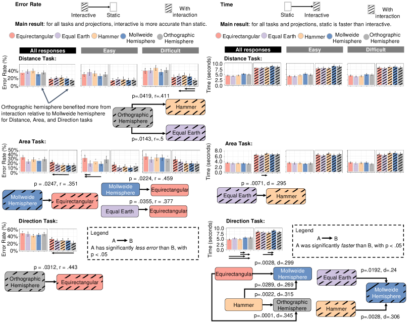
This diagram summarises the results of study 1 for error rate (left) and time (right). Significant differences between projections are shown as arrows. Significant differences between interactive and non-interactive conditions are omitted to improve readability. Error bars indicate 95% confidence intervals. Overall, equal earth and orthographic hemisphere performed well. The detailed statistical results and effect sizes can be found in Section A.1.
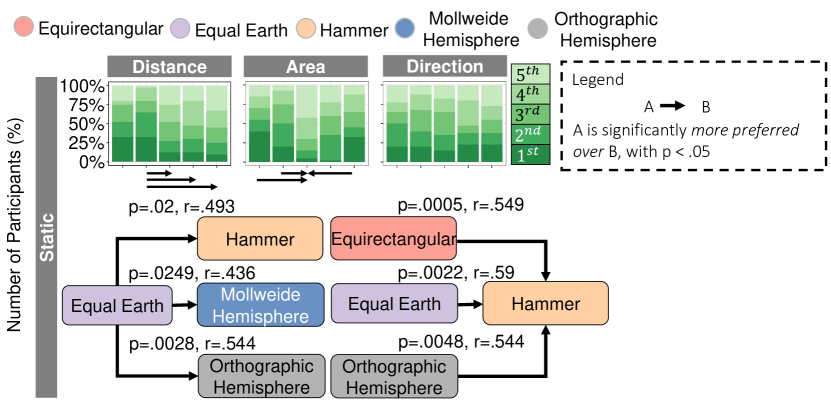
[Legend]This diagram shows the results of subjective user rank of map projections within the static group for three tested tasks. Lower rank indicates stronger preference. Arrows indicate statistical significance with . Overall, equal earth was found to be preferred over hemispheric projections for the distance comparison task, while hammer was preferred over by other projections for area comparison task.
4.8. Key Findings and Discussion
We report on the most significant findings for Distance Comparison
![[Uncaptioned image]](/html/2202.10845/assets/x59.png) , Area Comparison
, Area Comparison
![[Uncaptioned image]](/html/2202.10845/assets/x60.png) , and Direction estimation
, and Direction estimation
![[Uncaptioned image]](/html/2202.10845/assets/x61.png) visually in Figure 2 and Figure 3. Detailed statistic results and pairwise effect sizes are provided in the appendix: Section A.1 in the supplementary materials.
visually in Figure 2 and Figure 3. Detailed statistic results and pairwise effect sizes are provided in the appendix: Section A.1 in the supplementary materials.
Interaction improved error rate and is preferred over static map projections while taking participants longer time to complete (across all tasks).
This main effect was found statistically significant with moderate and large effect sizes in all three tested tasks (Figure 2, Section A.1: Figure 10, Figure 11-13). For Distance Comparison
![[Uncaptioned image]](/html/2202.10845/assets/x62.png) and Direction estimation
and Direction estimation
![[Uncaptioned image]](/html/2202.10845/assets/x63.png) , Interactive is always better (significantly less error and more preferred) than Static. For Area Comparison
, Interactive is always better (significantly less error and more preferred) than Static. For Area Comparison
![[Uncaptioned image]](/html/2202.10845/assets/x64.png) , Interactive has less error than the corresponding non-interactive projection but not necessarily all other non-interactive projections. Interactive was significantly preferred (moderate effects) for Hammer
, Interactive has less error than the corresponding non-interactive projection but not necessarily all other non-interactive projections. Interactive was significantly preferred (moderate effects) for Hammer
![[Uncaptioned image]](/html/2202.10845/assets/x65.png) and Equal Earth
and Equal Earth
![[Uncaptioned image]](/html/2202.10845/assets/x66.png) but not necessarily other projections for Area Comparison
but not necessarily other projections for Area Comparison
![[Uncaptioned image]](/html/2202.10845/assets/x67.png) . However, Interactive was significantly preferred in the overall user rank over Static (top horizontal bar in Section A.1: Figure 10) for Distance Comparison
. However, Interactive was significantly preferred in the overall user rank over Static (top horizontal bar in Section A.1: Figure 10) for Distance Comparison
![[Uncaptioned image]](/html/2202.10845/assets/x68.png) (large effects), Direction estimation
(large effects), Direction estimation
![[Uncaptioned image]](/html/2202.10845/assets/x69.png) (large effects) and Area Comparison
(large effects) and Area Comparison
![[Uncaptioned image]](/html/2202.10845/assets/x70.png) (moderate effects). Interactive is always slower (large effects) than Static (Figure 2-Time). Therefore, we accept H1-1, H1-2, H1-3.
(moderate effects). Interactive is always slower (large effects) than Static (Figure 2-Time). Therefore, we accept H1-1, H1-2, H1-3.
These results provide strong evidence that, with interactions, participants were able to find a better projection centre than the default one in a static map. Some participants explicitly mentioned the benefits of having interaction and their preference, e.g., “when moved [,the interactive conditions makes] it easier to judge when [the areas] were both placed in the middle in the least distorted part of the map.” (P20, Area-Interactive). and “The fact I couldn’t move the pictures was frustrating [for the static conditions] and I think I didn’t get many of the guesses right.” (P4, Direction-Static).
The choice of projections makes less difference and depends on tasks. However, overall, we found that equal earth and orthographi hemisphere performed well, while equirectangular may be a poor choice, organised in the following key findings.
In continuous projections, Equal Earth
![[Uncaptioned image]](/html/2202.10845/assets/x71.png) performed well in terms of Error for Area Comparison
performed well in terms of Error for Area Comparison
![[Uncaptioned image]](/html/2202.10845/assets/x72.png) , Time for Area Comparison
, Time for Area Comparison
![[Uncaptioned image]](/html/2202.10845/assets/x73.png) and Direction estimation
and Direction estimation
![[Uncaptioned image]](/html/2202.10845/assets/x74.png) , and Rank-Static for both Distance Comparison
, and Rank-Static for both Distance Comparison
![[Uncaptioned image]](/html/2202.10845/assets/x75.png) and Area Comparison
and Area Comparison
![[Uncaptioned image]](/html/2202.10845/assets/x76.png) . Equal Earth
. Equal Earth
![[Uncaptioned image]](/html/2202.10845/assets/x77.png) was not significantly worse than any other continuous projections. We found that for static projections, Equal Earth
was not significantly worse than any other continuous projections. We found that for static projections, Equal Earth
![[Uncaptioned image]](/html/2202.10845/assets/x78.png) tended to be more accurate (moderate effects) than Equirectangular
tended to be more accurate (moderate effects) than Equirectangular
![[Uncaptioned image]](/html/2202.10845/assets/x79.png) for Area-Easy. With interaction, Equal Earth
for Area-Easy. With interaction, Equal Earth
![[Uncaptioned image]](/html/2202.10845/assets/x80.png) tended to be faster (small effects) than Mollweide Hemisphere
tended to be faster (small effects) than Mollweide Hemisphere
![[Uncaptioned image]](/html/2202.10845/assets/x81.png) for Direction estimation
for Direction estimation
![[Uncaptioned image]](/html/2202.10845/assets/x82.png) , and Hammer
, and Hammer
![[Uncaptioned image]](/html/2202.10845/assets/x83.png) for Area-All (Figure 2-Time). Though the time results are statistically significant, the small effect sizes seem to indicate that the choice of projection makes a slight difference (Helske et al., 2021; Cockburn et al., 2020; in Human-Computer Interaction
Working Group, 2019; Schäfer and
Schwarz, 2019). For Rank-Static, Equal Earth
for Area-All (Figure 2-Time). Though the time results are statistically significant, the small effect sizes seem to indicate that the choice of projection makes a slight difference (Helske et al., 2021; Cockburn et al., 2020; in Human-Computer Interaction
Working Group, 2019; Schäfer and
Schwarz, 2019). For Rank-Static, Equal Earth
![[Uncaptioned image]](/html/2202.10845/assets/x84.png) was significantly preferred over Hammer
was significantly preferred over Hammer
![[Uncaptioned image]](/html/2202.10845/assets/x85.png) (moderate effect), Mollweide Hemisphere
(moderate effect), Mollweide Hemisphere
![[Uncaptioned image]](/html/2202.10845/assets/x86.png) (moderate effect), and Orthographic Hemisphere
(moderate effect), and Orthographic Hemisphere
![[Uncaptioned image]](/html/2202.10845/assets/x87.png) (large effect) for Distance Comparison
(large effect) for Distance Comparison
![[Uncaptioned image]](/html/2202.10845/assets/x88.png) (Figure 3-Distance). Furthermore, there is a strong evidence with important effects for Rank-Static that Equirectangular
(Figure 3-Distance). Furthermore, there is a strong evidence with important effects for Rank-Static that Equirectangular
![[Uncaptioned image]](/html/2202.10845/assets/x89.png) , Equal Earth
, Equal Earth
![[Uncaptioned image]](/html/2202.10845/assets/x90.png) , and Orthographic Hemisphere
, and Orthographic Hemisphere
![[Uncaptioned image]](/html/2202.10845/assets/x91.png) were significantly preferred over Hammer
were significantly preferred over Hammer
![[Uncaptioned image]](/html/2202.10845/assets/x92.png) (large effects) for Area Comparison
(large effects) for Area Comparison
![[Uncaptioned image]](/html/2202.10845/assets/x93.png) (Figure 3-Area). With interaction, there is no significant differences in user preference. This result is omitted from the paper and is available in Section A.1: Figure 9.
(Figure 3-Area). With interaction, there is no significant differences in user preference. This result is omitted from the paper and is available in Section A.1: Figure 9.
User preference of Static Equal Earth
![[Uncaptioned image]](/html/2202.10845/assets/x94.png) partially confirms Šavrič et al. (Šavric et al., 2015), who found Robinson projection (which is similarl to Equal Earth
partially confirms Šavrič et al. (Šavric et al., 2015), who found Robinson projection (which is similarl to Equal Earth
![[Uncaptioned image]](/html/2202.10845/assets/x95.png) ) was preferred over interrupted projections such as Mollweide Hemisphere
) was preferred over interrupted projections such as Mollweide Hemisphere
![[Uncaptioned image]](/html/2202.10845/assets/x96.png) and Goode Homolosine. This is also supported by our participants’ feedback where continuous maps are preferred over interrupted ones for Static (Section A.1.1).
and Goode Homolosine. This is also supported by our participants’ feedback where continuous maps are preferred over interrupted ones for Static (Section A.1.1).
Surprisingly, although Hammer
![[Uncaptioned image]](/html/2202.10845/assets/x97.png) is an equal-area projection, participants did not like it for area comparison in static maps (Figure 3-Area), This result partially differs from existing studies (Šavric et al., 2015) where poles represented as points were preferred over poles represented as lines.
We conjecture this effect is because when the target area is at the edges, the shapes are severely distorted, which makes it difficult to accurately accumulate its represented area, as participants mentioned “Equirectangular only was distorted from top to bottom, while [hammer was] also distorted on the sides.” (P31, Area-Static). More quotes can be found in Section A.1.1.
is an equal-area projection, participants did not like it for area comparison in static maps (Figure 3-Area), This result partially differs from existing studies (Šavric et al., 2015) where poles represented as points were preferred over poles represented as lines.
We conjecture this effect is because when the target area is at the edges, the shapes are severely distorted, which makes it difficult to accurately accumulate its represented area, as participants mentioned “Equirectangular only was distorted from top to bottom, while [hammer was] also distorted on the sides.” (P31, Area-Static). More quotes can be found in Section A.1.1.
In hemispheric projections, interaction reduced Error of Orthographic Hemisphere
![[Uncaptioned image]](/html/2202.10845/assets/x98.png) to a point that it tended to have a lower error rate than some interactive continuous projections for Distance-Hard and Direction, and not significantly slower than any interactive projections across all tasks. We found Orthographic Hemisphere
to a point that it tended to have a lower error rate than some interactive continuous projections for Distance-Hard and Direction, and not significantly slower than any interactive projections across all tasks. We found Orthographic Hemisphere
![[Uncaptioned image]](/html/2202.10845/assets/x99.png) performed well. Orthographic Hemisphere
performed well. Orthographic Hemisphere
![[Uncaptioned image]](/html/2202.10845/assets/x100.png) benefited more from interaction (large effects) for Error than Mollweide Hemisphere
benefited more from interaction (large effects) for Error than Mollweide Hemisphere
![[Uncaptioned image]](/html/2202.10845/assets/x101.png) (moderate effects) for Distance Comparison
(moderate effects) for Distance Comparison
![[Uncaptioned image]](/html/2202.10845/assets/x102.png) , while Orthographic Hemisphere
, while Orthographic Hemisphere
![[Uncaptioned image]](/html/2202.10845/assets/x103.png) benefited slightly more from interaction with similar effect sizes for Error than Mollweide Hemisphere
benefited slightly more from interaction with similar effect sizes for Error than Mollweide Hemisphere
![[Uncaptioned image]](/html/2202.10845/assets/x104.png) for Area Comparison
for Area Comparison
![[Uncaptioned image]](/html/2202.10845/assets/x105.png) and Direction estimation
and Direction estimation
![[Uncaptioned image]](/html/2202.10845/assets/x106.png) (Figure 2-Error, Section A.1: Figure 11-Figure 13). This is also supported by a strong evidence that Interactive Orthographic Hemisphere
(Figure 2-Error, Section A.1: Figure 11-Figure 13). This is also supported by a strong evidence that Interactive Orthographic Hemisphere
![[Uncaptioned image]](/html/2202.10845/assets/x107.png) has a lower error rate (large effects) than Equal Earth
has a lower error rate (large effects) than Equal Earth
![[Uncaptioned image]](/html/2202.10845/assets/x108.png) and a lower error rate (moderate effects) than Hammer
and a lower error rate (moderate effects) than Hammer
![[Uncaptioned image]](/html/2202.10845/assets/x109.png) for Distance-Hard (Figure 2-Error). By contrast, even with interaction, Mollweide Hemisphere
for Distance-Hard (Figure 2-Error). By contrast, even with interaction, Mollweide Hemisphere
![[Uncaptioned image]](/html/2202.10845/assets/x110.png) was still slower (small effects) than non-hemisphere for Direction estimation
was still slower (small effects) than non-hemisphere for Direction estimation
![[Uncaptioned image]](/html/2202.10845/assets/x111.png) (Figure 2-Time). Interactive Orthographic Hemisphere
(Figure 2-Time). Interactive Orthographic Hemisphere
![[Uncaptioned image]](/html/2202.10845/assets/x112.png) did not have a significantly lower error rate for Area Comparison
did not have a significantly lower error rate for Area Comparison
![[Uncaptioned image]](/html/2202.10845/assets/x113.png) than any interactive continuous projections, nor was there any significant difference in Rank-Interactive (Figure 9). Therefore, we reject H1-4, H1-5.
than any interactive continuous projections, nor was there any significant difference in Rank-Interactive (Figure 9). Therefore, we reject H1-4, H1-5.
It was surprising that Orthographic Hemisphere
![[Uncaptioned image]](/html/2202.10845/assets/x114.png) was comparable to other interactive projections for Area Comparison
was comparable to other interactive projections for Area Comparison
![[Uncaptioned image]](/html/2202.10845/assets/x115.png) since it is not an equal-area map projection. Meanwhile, the other non-equal-area map projection, i.e., Equirectangular
since it is not an equal-area map projection. Meanwhile, the other non-equal-area map projection, i.e., Equirectangular
![[Uncaptioned image]](/html/2202.10845/assets/x116.png) tended to produce more errors (moderate effects). We believe Orthographic Hemisphere
tended to produce more errors (moderate effects). We believe Orthographic Hemisphere
![[Uncaptioned image]](/html/2202.10845/assets/x117.png) were perceived as less distorted than the other projections due to the “natural” orthographic distortion, which is similar to viewing the sphere at infinite distance (e.g. as if through a telescope), echoed by our participants (Section A.1.1).
were perceived as less distorted than the other projections due to the “natural” orthographic distortion, which is similar to viewing the sphere at infinite distance (e.g. as if through a telescope), echoed by our participants (Section A.1.1).
Despite being hemispheric, Mollweide Hemisphere
![[Uncaptioned image]](/html/2202.10845/assets/x118.png) was found to be less intuitive for some tasks by participants (Section A.1.1). We conjecture that there is a slight distortion near the edge of two circles which may make it confusing when centring the region of interest. However, there were also participants who did not like the hemispheric projections due to the need to inspect two separated spheres and instead they preferred the continuous maps in the non-hemispheric group (Section A.1.1).
was found to be less intuitive for some tasks by participants (Section A.1.1). We conjecture that there is a slight distortion near the edge of two circles which may make it confusing when centring the region of interest. However, there were also participants who did not like the hemispheric projections due to the need to inspect two separated spheres and instead they preferred the continuous maps in the non-hemispheric group (Section A.1.1).
Even with interaction, Equirectangular
![[Uncaptioned image]](/html/2202.10845/assets/x119.png) still tended to perform poorly in terms of Error for Area Comparison
still tended to perform poorly in terms of Error for Area Comparison
![[Uncaptioned image]](/html/2202.10845/assets/x120.png) and Direction estimation
and Direction estimation
![[Uncaptioned image]](/html/2202.10845/assets/x121.png) . Overall, for static projections, Equirectangular
. Overall, for static projections, Equirectangular
![[Uncaptioned image]](/html/2202.10845/assets/x122.png) tended to have a higher error rate (moderate effects) than Equal Earth
tended to have a higher error rate (moderate effects) than Equal Earth
![[Uncaptioned image]](/html/2202.10845/assets/x123.png) and Mollweide Hemisphere
and Mollweide Hemisphere
![[Uncaptioned image]](/html/2202.10845/assets/x124.png) (Figure 2-Error).
To our surprise, with the ability to rotate to centre the region of interest, Equirectangular
(Figure 2-Error).
To our surprise, with the ability to rotate to centre the region of interest, Equirectangular
![[Uncaptioned image]](/html/2202.10845/assets/x125.png) still tended to be outperformed for Error by Mollweide Hemisphere
still tended to be outperformed for Error by Mollweide Hemisphere
![[Uncaptioned image]](/html/2202.10845/assets/x126.png) (moderate effect) for Area-All and by Orthographic Hemisphere
(moderate effect) for Area-All and by Orthographic Hemisphere
![[Uncaptioned image]](/html/2202.10845/assets/x127.png) (moderate effect) for Direction estimation
(moderate effect) for Direction estimation
![[Uncaptioned image]](/html/2202.10845/assets/x128.png) (Figure 2-Error). This partially confirms Hennerdal et al.’s static map study where Static Equirectangular
(Figure 2-Error). This partially confirms Hennerdal et al.’s static map study where Static Equirectangular
![[Uncaptioned image]](/html/2202.10845/assets/x129.png) was found confusing when estimating the airplane route that wraps around (Hennerdal, 2015). We conjecture that Equirectangular
was found confusing when estimating the airplane route that wraps around (Hennerdal, 2015). We conjecture that Equirectangular
![[Uncaptioned image]](/html/2202.10845/assets/x130.png) features the most distortion of all tested projections due to the high level of stretching near the poles, supported by participants’ feedback (Section A.1.1).
features the most distortion of all tested projections due to the high level of stretching near the poles, supported by participants’ feedback (Section A.1.1).
4.9. Limitations
The statistically significant results with large effect sizes provide a strong evidence that adding the spherical rotation interaction to static maps improves the accuracy, is strongly preferred, but at the cost of longer completion time across all tasks. However, despite being statistically significant, the differences between projections within static or interactive groups are of small sizes for Time, medium-sized for Error and large-sized for Rank-Static-Area (Figure 2, Figure 3). Although medium-sized differences in Error are likely to be noticeable in practical applications, these results only allow us to say Equal Earth
![[Uncaptioned image]](/html/2202.10845/assets/x131.png) and Orthographic Hemisphere
and Orthographic Hemisphere
![[Uncaptioned image]](/html/2202.10845/assets/x132.png) performed well for some tasks (Helske et al., 2021; Cockburn et al., 2020; in Human-Computer Interaction
Working Group, 2019; Schäfer and
Schwarz, 2019).
performed well for some tasks (Helske et al., 2021; Cockburn et al., 2020; in Human-Computer Interaction
Working Group, 2019; Schäfer and
Schwarz, 2019).
Although the results show statistically significant differences between the selected hemispheric and non-hemispheric projections across all tasks for Error, the results do not allow us to say that hemispheric projections are always more accurate than non-hemispheric projections. Arguably, the poor performance of non-hemispheric projections for Area Comparison
![[Uncaptioned image]](/html/2202.10845/assets/x133.png) and Direction estimation
and Direction estimation
![[Uncaptioned image]](/html/2202.10845/assets/x134.png) is entirely based on Equirectangular
is entirely based on Equirectangular
![[Uncaptioned image]](/html/2202.10845/assets/x135.png) compared with either Mollweide Hemisphere
compared with either Mollweide Hemisphere
![[Uncaptioned image]](/html/2202.10845/assets/x136.png) or Orthographic Hemisphere
or Orthographic Hemisphere
![[Uncaptioned image]](/html/2202.10845/assets/x137.png) . If the results from the Equirectangular
. If the results from the Equirectangular
![[Uncaptioned image]](/html/2202.10845/assets/x138.png) were not considered, the hemispheric and non-hemispheric projections seem to have very similar error rates for Area Comparison
were not considered, the hemispheric and non-hemispheric projections seem to have very similar error rates for Area Comparison
![[Uncaptioned image]](/html/2202.10845/assets/x139.png) and Direction estimation
and Direction estimation
![[Uncaptioned image]](/html/2202.10845/assets/x140.png) . Similarly, the results do not allow us to say that non-hemispheric projections are always faster, as this seems only based on Mollweide Hemisphere
. Similarly, the results do not allow us to say that non-hemispheric projections are always faster, as this seems only based on Mollweide Hemisphere
![[Uncaptioned image]](/html/2202.10845/assets/x141.png) being significantly slower (small effects) than some non-hemispheric projections for Static and Interactive for the direction tasks.
being significantly slower (small effects) than some non-hemispheric projections for Static and Interactive for the direction tasks.
Surprisingly, unlike the study by Yang et al. (Yang et al., 2018), we did not identify superior performance of Orthographic Hemisphere
![[Uncaptioned image]](/html/2202.10845/assets/x142.png) compared to other map projections.
We conjectured that rendering Orthographic Hemisphere
compared to other map projections.
We conjectured that rendering Orthographic Hemisphere
![[Uncaptioned image]](/html/2202.10845/assets/x143.png) on a 2D flat display produced different effectiveness in perception and interaction compared to Yang et al’s 3D globes in VR.
Meanwhile, although not in all tasks, Orthographic Hemisphere
on a 2D flat display produced different effectiveness in perception and interaction compared to Yang et al’s 3D globes in VR.
Meanwhile, although not in all tasks, Orthographic Hemisphere
![[Uncaptioned image]](/html/2202.10845/assets/x144.png) demonstrated some advantages for Distance Comparison
demonstrated some advantages for Distance Comparison
![[Uncaptioned image]](/html/2202.10845/assets/x145.png) , Direction estimation
, Direction estimation
![[Uncaptioned image]](/html/2202.10845/assets/x146.png) and benefited more from interaction than Mollweide Hemisphere
and benefited more from interaction than Mollweide Hemisphere
![[Uncaptioned image]](/html/2202.10845/assets/x147.png) for Error ( Section 4.8).
for Error ( Section 4.8).
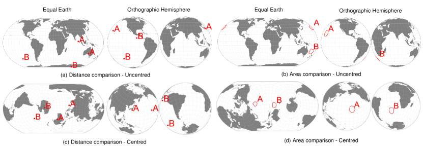
[]This diagram shows examples of study trials of Equal Earth and Orthographic Hemisphere for distance and area comparison tasks. Static (a,b) may result in uncentred view. Interactive (c,d) allows a user to drag the map to find the best angle (centred) to answer the task.
5. Spherical Network Layout
In Study 1, we found that interaction (panning by spherical rotation) makes spherical geographic projections overwhelmingly more accurate for distance, area and direction tasks. A question, however, is whether such 2D interactive spherical projections are also useful for abstract data. As discussed in Section 2, there has been a number of systems using immersive environments to visualise network data on 3D spherical surfaces or straightforward perspective projections of spheres. Various advantages have been claimed to the opportunities for embedding a network layout in the surface of a sphere—without boundary—such as centring any node of interest in the layout (Brath and MacMurchy, 2012; Perry et al., 2020; Rodighiero, 2020), improving readability by reducing link crossings using the third dimension (Ware and Mitchell, 2008), and stereoscopy outperforms standard 2D layouts for highly overlapping clustered graphs (Greffard et al., 2011). However, the visualisation design literature cautions against such use of 3D if there are layout approaches better suited to the plane (Munzner, 2014, Ch. 6).
Further, there are obvious disadvantages to projection, since all projections introduce some degree of distortion and discontinuity. There are therefore three questions:
RQ1: Which of the most promising projections from our first study are the best for visualising the layout of a node-link diagram?
RQ2: Does a spherical projection have advantages in supporting network understanding tasks compared to conventional 2D layouts?
RQ3: Does a spherical projection provide perceptual benefits compared with arrangements on other 3D topologies, such as a torus?
Before we can answer these questions, we need techniques to create effective layouts of complex network data on a spherical surface and to orient the projections optimally in 2D.
5.1. Plane, Spherical and Toroidal Stress Minisation
The tasks we investigate are cluster understanding tasks and path following. Network clusters are loosely defined as subsets of nodes within the graph that are more highly connected to each other than would be expected from chance connection of edges within a graph of that density. More formally, a clustered graph has disjoint sets of nodes with positive modularity, a metric due to Newman which directly measures the connectivity of given clusters compared to overall connectivity (Newman, 2006). To support cluster understanding tasks we need a layout method which provides good separation between these clusters.
To support path following tasks, we need a layout method which spreads the network out relatively uniformly according to connectivity. This will help minimise crossings between edges.
We follow recent work (Chen et al., 2020, 2021a; Zheng et al., 2018) which adopted a stress minimising approach. Stress-minimisation is a commonly used variant of a general-purpose force-directed layout and does a reasonable job of satisfying both of these readability criteria (Huang et al., 2009; Purchase, 2002). The stress metric () for a given layout of a graph with nodes in a 2D plane is defined (following Gansner et al. (Gansner et al., 2004)) as:
where: is the ideal separation between the 2D positions ( and ) of a pair of nodes taken as the all-pairs shortest path length between them; is the actual distance between nodes and (in the plane this is Euclidean distance); and is a weighting which is applied to trade-off between the importance of short and long ideal distances, we follow the standard choice of .
We follow previous recent work by Perry et al. (Perry et al., 2020), in adapting stress-based graph layout to a spherical surface by redefining to arc-length on the sphere surface, or (assuming a unit sphere):
where and are the 3D vector offsets of nodes and respectively from the sphere centroid and is the inner product. For the layout to be reasonable, the ideal lengths must be chosen such that the largest corresponds to the largest separation possible on the unit sphere surface, which is . Thus, we set the ideal length of all edges to .
The other layout against which we compare is a projection of a 3D torus, which, as discussed in Section 2 has recently been shown to provide better separation between clusters than a flat (conventional) 2D layout by Chen et al. (Chen et al., 2021a). We use the same layout method which is also based on stress in the 2D plane but which, for each node pair, requires selecting the stress term from the set of 9 possible torus adjacencies for that pair which contributes the least to the overall stress:
While Perry et al. follow the multi-dimensional scaling literature in using a majorization method to minimise , we follow Chen et al. (Chen et al., 2021a) in using the stochastic pairwise gradient descent approach developed by (Zheng et al., 2018) which can be adapted straightforwardly and effectively to obtain layout for all of .
Note that the layouts which result from minimising and are already in 2D. For the spherical layout obtained by minimising , we use either Orthographic Hemisphere
![[Uncaptioned image]](/html/2202.10845/assets/x149.png) or Equal Earth
or Equal Earth
![[Uncaptioned image]](/html/2202.10845/assets/x150.png) projections to generate the stimuli for our study. The detailed pseudocode of our algorithms are available in https://github.com/Kun-Ting/gansdawrap.
projections to generate the stimuli for our study. The detailed pseudocode of our algorithms are available in https://github.com/Kun-Ting/gansdawrap.
5.2. Auto-pan Algorithms
 - No pan
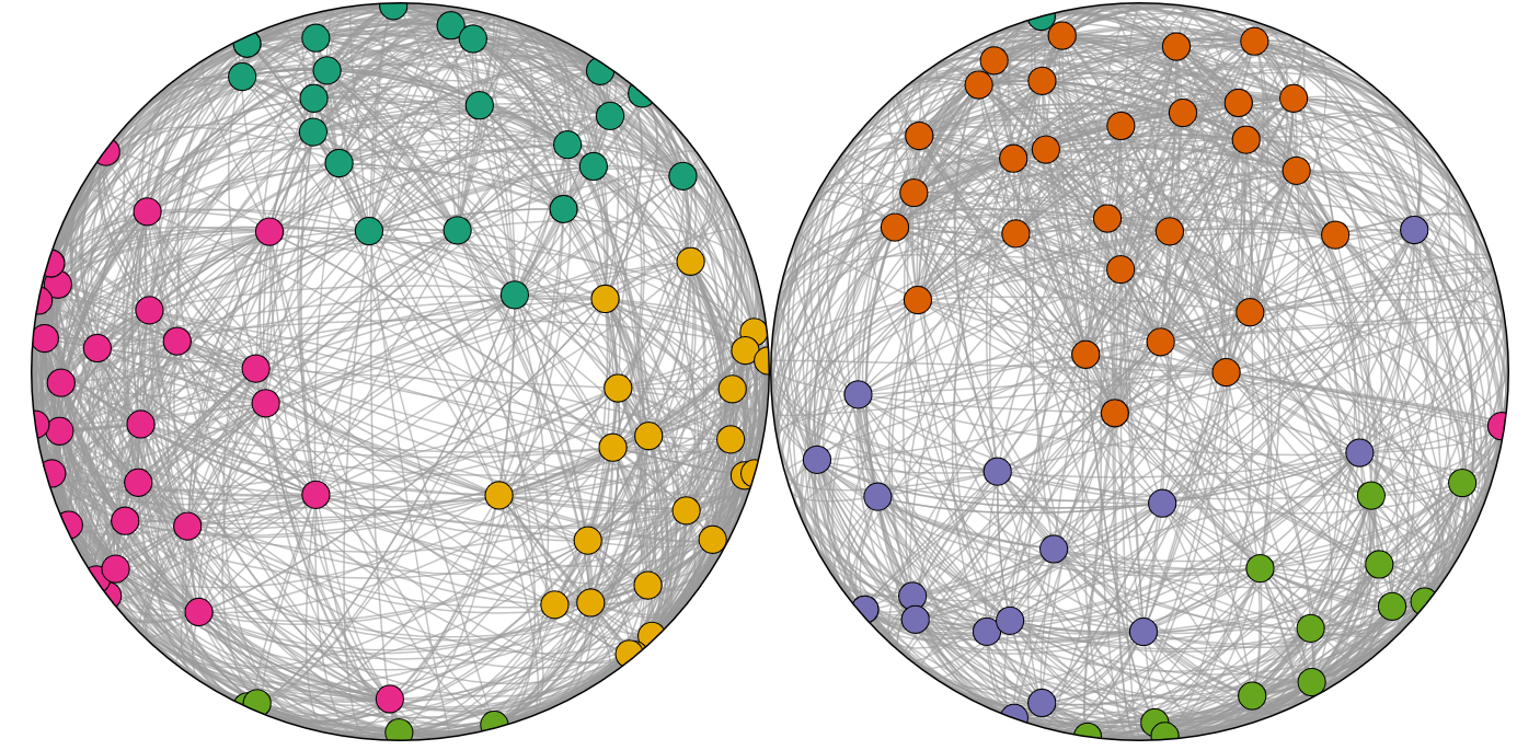
 - Best pan
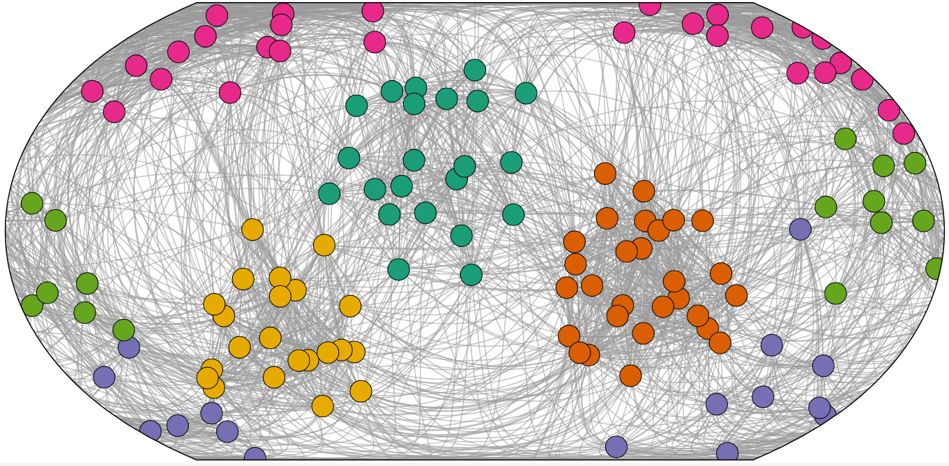
 - No pan (left), edge pixel mask (inset)
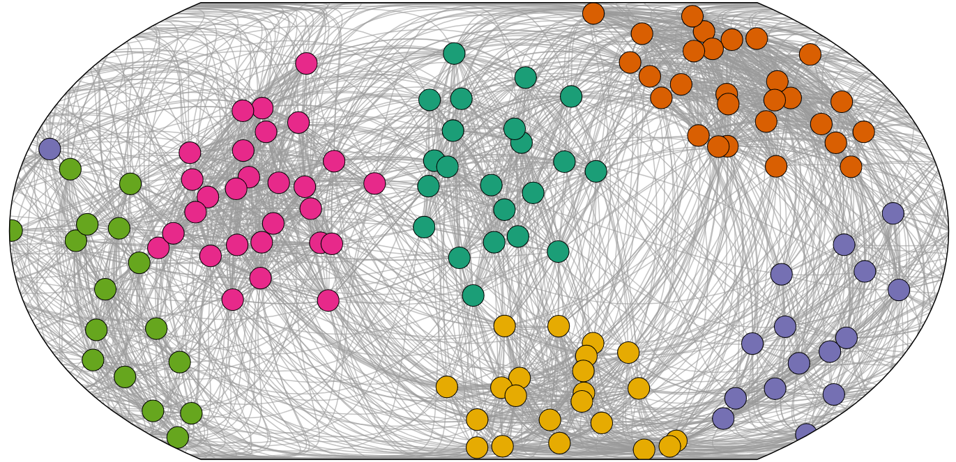
 - Best pan (left), edge pixel mask (inset)
 (a) or at the boundaries in Equal Earth
 (c). Auto-pan reduces the number of wrapped edges and thereby brings the clusters together (b) and (d).
[Example of automatic panning]This diagram shows examples of automatic panning. It shows before and after applying our auto-pan algorithms of a graph with six clusters differentiated by colour. Without auto-pan, clusters can be split across the hemispheres in Orthographic Hemisphere
![[Uncaptioned image]](/html/2202.10845/assets/x166.png) (a) or at the boundaries in Equal Earth
(a) or at the boundaries in Equal Earth
![[Uncaptioned image]](/html/2202.10845/assets/x167.png) (c). Auto-pan reduces the number of wrapped edges and thereby brings the clusters together (b) and (d).
(c). Auto-pan reduces the number of wrapped edges and thereby brings the clusters together (b) and (d).
For toroidal network layout, Chen et al. introduced an algorithm to automatically pan the toroidal layout horizontally and vertically to minimise the number of edges which wrap around at the boundaries (Chen et al., 2021a). Spherical projections can also suffer when too many edges are split across the boundaries. Furthermore, edges are more distorted in spherical projections when they are near the edges. Therefore, for fair comparison with toroidal layouts, it was necessary to find a method to auto-rotate the sphere to reduce the numbers of such edges. However, while the toroidal auto-panning algorithm can be done with horizontal and vertical scans (linear time in the number of edges), the spherical layout does not permit such a trivial search algorithm. We therefore develop heuristics to perform auto-rotate for the spherical projections. For both, we choose a simple stochastic method of randomly selecting a large number (e.g., 1000 iterations) of three-axis spherical rotation angle triples and choosing the triple for which edges crossing (or near) boundaries is minimised.
For Orthographic Hemisphere
![[Uncaptioned image]](/html/2202.10845/assets/x168.png) projection this crossing number is trivial to count precisely. Simply, for all pairs of nodes if the nodes are not on the same face, then they must cross a boundary. A suboptimal Orthographic Hemisphere
projection this crossing number is trivial to count precisely. Simply, for all pairs of nodes if the nodes are not on the same face, then they must cross a boundary. A suboptimal Orthographic Hemisphere
![[Uncaptioned image]](/html/2202.10845/assets/x169.png) projection rotation, and the result of autorotation to minimise this crossing count is shown in 5(d)(a) and 5(d)(b), respectively.
projection rotation, and the result of autorotation to minimise this crossing count is shown in 5(d)(a) and 5(d)(b), respectively.
For Equal Earth
![[Uncaptioned image]](/html/2202.10845/assets/x170.png) projection the edges are curved and so determining those that cross the boundary for a given geo-rotation is more complex. Further, in this projection edges near the periphery are significantly more distorted than those near the centre, so even visually determining if an edge that comes close to the boundary continues on the same side of the projection or wraps around to the other side is not easy. Thus, instead of counting boundary crossings, we penalise all edges which come close to the boundaries. To compute the penalty we analyse the periphery of a monochrome bitmap of the projected edge paths. The penalty is then simply the number of black pixels. Example masked bitmaps are shown for sub-optimal and more-optimal rotations of an Equal Earth
projection the edges are curved and so determining those that cross the boundary for a given geo-rotation is more complex. Further, in this projection edges near the periphery are significantly more distorted than those near the centre, so even visually determining if an edge that comes close to the boundary continues on the same side of the projection or wraps around to the other side is not easy. Thus, instead of counting boundary crossings, we penalise all edges which come close to the boundaries. To compute the penalty we analyse the periphery of a monochrome bitmap of the projected edge paths. The penalty is then simply the number of black pixels. Example masked bitmaps are shown for sub-optimal and more-optimal rotations of an Equal Earth
![[Uncaptioned image]](/html/2202.10845/assets/x171.png) projection in 5(d)(c) and 5(d)(d), respectively.
projection in 5(d)(c) and 5(d)(d), respectively.
5.3. Automatic Panning Results
We conducted a small empirical analysis of the Auto-Pan algorithm to assess the numbers of links wrapped for Orthographic Hemisphere
![[Uncaptioned image]](/html/2202.10845/assets/x172.png) and the number of pixels (higher values indicate less wrappings) at the boundary of Equal Earth
and the number of pixels (higher values indicate less wrappings) at the boundary of Equal Earth
![[Uncaptioned image]](/html/2202.10845/assets/x173.png) projections compared to 10 random rotations. Across 10 study graphs (Small+Easy, Small+Hard) used in our cluster understanding tasks, we found for Orthographic Hemisphere
projections compared to 10 random rotations. Across 10 study graphs (Small+Easy, Small+Hard) used in our cluster understanding tasks, we found for Orthographic Hemisphere
![[Uncaptioned image]](/html/2202.10845/assets/x174.png) , the mean crossing count for random rotations was 262.16. With automatic panning, this number was improved by and was reduced to 208.7. For Equal Earth
, the mean crossing count for random rotations was 262.16. With automatic panning, this number was improved by and was reduced to 208.7. For Equal Earth
![[Uncaptioned image]](/html/2202.10845/assets/x175.png) , our automatic panning increased number of pixels at the boundary region by (Section A.2: Table 2). We found these auto-pan algorithms resulted in a noticeable improvement in keeping clusters from being separated, as evidenced in 5(d).
, our automatic panning increased number of pixels at the boundary region by (Section A.2: Table 2). We found these auto-pan algorithms resulted in a noticeable improvement in keeping clusters from being separated, as evidenced in 5(d).
6. Study 2: network projection readability
In Study 1, we found Equal Earth
![[Uncaptioned image]](/html/2202.10845/assets/x176.png) , had advantages in terms of error rate, time, and subjective user feedback. Orthographic Hemisphere
, had advantages in terms of error rate, time, and subjective user feedback. Orthographic Hemisphere
![[Uncaptioned image]](/html/2202.10845/assets/x177.png) , despite being an interrupted projection, benefited more from interaction than Mollweide Hemisphere
, despite being an interrupted projection, benefited more from interaction than Mollweide Hemisphere
![[Uncaptioned image]](/html/2202.10845/assets/x178.png) and performed well in terms of error rate for distance and direction tasks (Section 4.8).
Based on these findings, we chose interactive Equal Earth
and performed well in terms of error rate for distance and direction tasks (Section 4.8).
Based on these findings, we chose interactive Equal Earth
![[Uncaptioned image]](/html/2202.10845/assets/x179.png) and Orthographic Hemisphere
and Orthographic Hemisphere
![[Uncaptioned image]](/html/2202.10845/assets/x180.png) , to understand their performance in visualising networks.
We compare these spherical projections to standard flat graph layout (Flat
, to understand their performance in visualising networks.
We compare these spherical projections to standard flat graph layout (Flat
![[Uncaptioned image]](/html/2202.10845/assets/sections/flatgraph.png) ) and a projection of a Torus
) and a projection of a Torus
![[Uncaptioned image]](/html/2202.10845/assets/x181.png) geometry (Chen
et al., 2021a). Our study was run in a similar way to Study 1 and included a new set of 96 participants through the Prolific platform.
geometry (Chen
et al., 2021a). Our study was run in a similar way to Study 1 and included a new set of 96 participants through the Prolific platform.
6.1. Techniques & Setup
The techniques in our study are Flat
, Torus
![[Uncaptioned image]](/html/2202.10845/assets/x182.png) , Equal Earth
, Equal Earth
![[Uncaptioned image]](/html/2202.10845/assets/x183.png) , and Orthographic Hemisphere
, and Orthographic Hemisphere
![[Uncaptioned image]](/html/2202.10845/assets/x184.png) . Layouts are computed as described in Section 5.
All the techniques support interactive panning except for Flat
which does not wrap around.
The area of the rectangular bounding box of each technique condition is the same. For Flat
and Torus
. Layouts are computed as described in Section 5.
All the techniques support interactive panning except for Flat
which does not wrap around.
The area of the rectangular bounding box of each technique condition is the same. For Flat
and Torus
![[Uncaptioned image]](/html/2202.10845/assets/x185.png) , the resolution is fixed at pixels, and for Equal Earth
, the resolution is fixed at pixels, and for Equal Earth
![[Uncaptioned image]](/html/2202.10845/assets/x186.png) and Orthographic Hemisphere
and Orthographic Hemisphere
![[Uncaptioned image]](/html/2202.10845/assets/x187.png) , the resolution is fixed at pixels.
For Cluster Number
, the resolution is fixed at pixels.
For Cluster Number
![[Uncaptioned image]](/html/2202.10845/assets/x188.png) , we did not color clusters to not reveal any graph structure.
, we did not color clusters to not reveal any graph structure.
6.2. Tasks
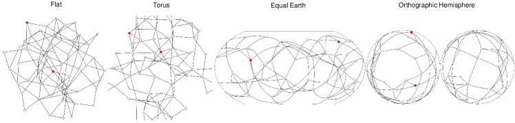 \Description
[]This diagram shows an example of one study graph laid out using 4 techniques described in Section 5.1 for shortest path number task. The shortest path length is 3 in this example. Participants were provided with interactive panning for spherical and toroidal layouts to explore the network.
 . The shortest path length is 3 in this example. Participants were provided with interactive panning for spherical and toroidal layouts to explore the network.
We selected two representative network visualisation tasks, inspired by existing work comparing 2D layout of 3D surface topology (Chen et al., 2021a, 2020) and task taxonomies (Lee et al., 2006; Saket et al., 2014).
Cluster Number
![[Uncaptioned image]](/html/2202.10845/assets/x192.png) : Please count the number of clusters in this graph. Participants answered through radio buttons: choices ranged from 1 to 10. We created a quality control trial for each condition with two clusters with clearly marked boundaries to assess participants’ attention. Participants who did not answer these trials correctly were excluded. An example of 5 clusters from Large+Easy graphs (Section 6.3) using 4 different layouts is shown in Figure 1-Bottom.
: Please count the number of clusters in this graph. Participants answered through radio buttons: choices ranged from 1 to 10. We created a quality control trial for each condition with two clusters with clearly marked boundaries to assess participants’ attention. Participants who did not answer these trials correctly were excluded. An example of 5 clusters from Large+Easy graphs (Section 6.3) using 4 different layouts is shown in Figure 1-Bottom.
Shortest Path Number
![[Uncaptioned image]](/html/2202.10845/assets/x193.png) : What is the shortest path length between the red nodes?: Participants were required to count the smallest number of links between two red nodes. Radio buttons allowed them to answer between 1 to 6. Again, we created a quality control trial for each layout condition, with shortest path length two and links on the path highlighted in red. An example of Easy graphs (Section 6.3) using 4 different layouts is shown in Figure 6.
: What is the shortest path length between the red nodes?: Participants were required to count the smallest number of links between two red nodes. Radio buttons allowed them to answer between 1 to 6. Again, we created a quality control trial for each layout condition, with shortest path length two and links on the path highlighted in red. An example of Easy graphs (Section 6.3) using 4 different layouts is shown in Figure 6.
6.3. Data Sets
We prepared a separate graph corpus for each task, full details and stimuli are presented in our supplementary material. For Cluster Number
![[Uncaptioned image]](/html/2202.10845/assets/x194.png) , we use graphs from Chen et al. (Chen
et al., 2021a), generated using algorithms designed to simulate real-world community structures in graphs (Brandes
et al., 2003; Fortunato, 2010).
Graphs are grouped by two variables: difficulty in terms of graph modularity (Newman, 2006) (Easy: modularity=0.4, Hard: modularity=0.3) and size (2 levels: Small: 68-80 nodes, 710-925 links, and Large: 126-134 nodes, 2310-2590 links). The number of clusters is between 4 and 7.
For Shortest Path Number
, we use graphs from Chen et al. (Chen
et al., 2021a), generated using algorithms designed to simulate real-world community structures in graphs (Brandes
et al., 2003; Fortunato, 2010).
Graphs are grouped by two variables: difficulty in terms of graph modularity (Newman, 2006) (Easy: modularity=0.4, Hard: modularity=0.3) and size (2 levels: Small: 68-80 nodes, 710-925 links, and Large: 126-134 nodes, 2310-2590 links). The number of clusters is between 4 and 7.
For Shortest Path Number
![[Uncaptioned image]](/html/2202.10845/assets/x195.png) the clustered graphs were too dense, so we generated sparser graphs using scale-free models (Barabási and
Albert, 1999; Watts and
Strogatz, 1998).
We chose graphs with two levels of density (Easy: 0.075, and Hard: 0.11) with 50 to 57 nodes.
The shortest path length varied between 1 and 4.
the clustered graphs were too dense, so we generated sparser graphs using scale-free models (Barabási and
Albert, 1999; Watts and
Strogatz, 1998).
We chose graphs with two levels of density (Easy: 0.075, and Hard: 0.11) with 50 to 57 nodes.
The shortest path length varied between 1 and 4.
6.4. Hypotheses
Hypotheses were pre-registered with the Open Science Foundation: https://osf.io/equhp.
H2-1: Equal Earth
![[Uncaptioned image]](/html/2202.10845/assets/x196.png) and Torus
and Torus
![[Uncaptioned image]](/html/2202.10845/assets/x197.png) have better task effectiveness for Cluster Number
have better task effectiveness for Cluster Number
![[Uncaptioned image]](/html/2202.10845/assets/x198.png) (in terms of time and error) than Orthographic Hemisphere
(in terms of time and error) than Orthographic Hemisphere
![[Uncaptioned image]](/html/2202.10845/assets/x199.png) (RQ1, RQ3) or Flat
(RQ2). While Orthographic Hemisphere
(RQ1, RQ3) or Flat
(RQ2). While Orthographic Hemisphere
![[Uncaptioned image]](/html/2202.10845/assets/x200.png) performed well in Study 1, our pilot studies for Cluster Number
performed well in Study 1, our pilot studies for Cluster Number
![[Uncaptioned image]](/html/2202.10845/assets/x201.png) revealed that cuts and distortion of clusters at the borders made them hard to count. For (RQ2), the inspiration was based on prior cluster readability studies (Chen
et al., 2021a).
revealed that cuts and distortion of clusters at the borders made them hard to count. For (RQ2), the inspiration was based on prior cluster readability studies (Chen
et al., 2021a).
H2-2: Participants will prefer Equal Earth
![[Uncaptioned image]](/html/2202.10845/assets/x202.png) and Torus
and Torus
![[Uncaptioned image]](/html/2202.10845/assets/x203.png) to Orthographic Hemisphere
to Orthographic Hemisphere
![[Uncaptioned image]](/html/2202.10845/assets/x204.png) (RQ1, RQ3) or Flat
(RQ2) for Cluster Number
(RQ1, RQ3) or Flat
(RQ2) for Cluster Number
![[Uncaptioned image]](/html/2202.10845/assets/x205.png) . Our early pilots indicating this preference — perhaps for the same reasons as above and inspiration from existing studies (Chen
et al., 2021a).
. Our early pilots indicating this preference — perhaps for the same reasons as above and inspiration from existing studies (Chen
et al., 2021a).
H2-3: Torus
![[Uncaptioned image]](/html/2202.10845/assets/x206.png) has better task effectiveness (in terms of time and error) for Shortest Path Number
has better task effectiveness (in terms of time and error) for Shortest Path Number
![[Uncaptioned image]](/html/2202.10845/assets/x207.png) than Flat
Equal Earth
than Flat
Equal Earth
![[Uncaptioned image]](/html/2202.10845/assets/x208.png) or Orthographic Hemisphere
or Orthographic Hemisphere
![[Uncaptioned image]](/html/2202.10845/assets/x209.png) (RQ3). This assumption is based on pilot studies and prior studies indicating curved links might hamper path tracing tasks (Du
et al., 2017; Xu
et al., 2012).
(RQ3). This assumption is based on pilot studies and prior studies indicating curved links might hamper path tracing tasks (Du
et al., 2017; Xu
et al., 2012).
H2-4: Participants will prefer Torus
![[Uncaptioned image]](/html/2202.10845/assets/x210.png) to Flat
, Equal Earth
to Flat
, Equal Earth
![[Uncaptioned image]](/html/2202.10845/assets/x211.png) or Orthographic Hemisphere
or Orthographic Hemisphere
![[Uncaptioned image]](/html/2202.10845/assets/x212.png) (RQ3) for Shortest Path Number
(RQ3) for Shortest Path Number
![[Uncaptioned image]](/html/2202.10845/assets/x213.png) . Again, it was assumed due to distortion of links.
. Again, it was assumed due to distortion of links.
6.5. Experimental Design
We use a within-subjects design for each task with 4 techniques. Each participant was randomly assigned one of the tasks by the experimental software. For Cluster Number
![[Uncaptioned image]](/html/2202.10845/assets/x214.png) , we used 2 levels of difficulty (Easy, Hard) 2 sizes (Small, Large) 5 repetitions. We randomly inserted one additional quality control trial to each layout condition. Each recorded trial had a timeout of 20 seconds to prevent participants from trying to perform precise link counting. This leaves us with a total of 80 recorded trials per participant. We counterbalanced the order of the techniques using a full-factorial design. The order of each level of difficulty and size in each technique was the same: Small+EasyLarge+Easy Small+HardLarge+Hard. The order of trials for each technique within each level was randomised.
, we used 2 levels of difficulty (Easy, Hard) 2 sizes (Small, Large) 5 repetitions. We randomly inserted one additional quality control trial to each layout condition. Each recorded trial had a timeout of 20 seconds to prevent participants from trying to perform precise link counting. This leaves us with a total of 80 recorded trials per participant. We counterbalanced the order of the techniques using a full-factorial design. The order of each level of difficulty and size in each technique was the same: Small+EasyLarge+Easy Small+HardLarge+Hard. The order of trials for each technique within each level was randomised.
For Shortest Path Number
![[Uncaptioned image]](/html/2202.10845/assets/x215.png) , we used 2 levels of difficulty (Easy, Hard) 8 repetitions. There were 2 repetitions of each shortest path length per level. One additional quality control trial was added for each layout condition. This leaves us with a total of 64 trials per participant. Each recorded trial had a timeout of 30 seconds, informed by pilot studies. The order of each level of difficulty in each technique was the same: Easy Hard. The order of trials for each technique within each level was randomised.
, we used 2 levels of difficulty (Easy, Hard) 8 repetitions. There were 2 repetitions of each shortest path length per level. One additional quality control trial was added for each layout condition. This leaves us with a total of 64 trials per participant. Each recorded trial had a timeout of 30 seconds, informed by pilot studies. The order of each level of difficulty in each technique was the same: Easy Hard. The order of trials for each technique within each level was randomised.
6.6. Participants and Procedures
Setup and inclusion criteria for participants were the same as for Study 1. We recorded 96 participants (37 female, 59 male, age range [18,50]) who passed the attention check trials, completed the training and recorded trials. This comprised 2 fully counterbalanced blocks of participants (24 2 2 tasks). They ranked their familiarity with network diagrams as: 9 often seeing network diagrams; 62 occasionally; and 25 never.
For Cluster Number
![[Uncaptioned image]](/html/2202.10845/assets/x216.png) , each participant was presented with a tutorial explaining the concept of network clusters. For Torus
, each participant was presented with a tutorial explaining the concept of network clusters. For Torus
![[Uncaptioned image]](/html/2202.10845/assets/x217.png) Equal Earth
Equal Earth
![[Uncaptioned image]](/html/2202.10845/assets/x218.png) , and Orthographic Hemisphere
, and Orthographic Hemisphere
![[Uncaptioned image]](/html/2202.10845/assets/x219.png) , animated videos were given to demonstrate the interactive panning or rotation. Each participant then completed training trials, similar to the recorded trials.
For Shortest Path Number
, animated videos were given to demonstrate the interactive panning or rotation. Each participant then completed training trials, similar to the recorded trials.
For Shortest Path Number
![[Uncaptioned image]](/html/2202.10845/assets/x220.png) , each participant was presented with a tutorial explaining the concept. For Torus
, each participant was presented with a tutorial explaining the concept. For Torus
![[Uncaptioned image]](/html/2202.10845/assets/x221.png) , Equal Earth
, Equal Earth
![[Uncaptioned image]](/html/2202.10845/assets/x222.png) , Orthographic Hemisphere
, Orthographic Hemisphere
![[Uncaptioned image]](/html/2202.10845/assets/x223.png) , animated videos were given to demonstrate the interactive panning or rotation.
Training trials were similar to the recorded trials.
, animated videos were given to demonstrate the interactive panning or rotation.
Training trials were similar to the recorded trials.
Specific instructions given for each task is available in the supplementary material333An online demonstration of the study is available: https://observablehq.com/@kun-ting/gansdawrap.
6.7. Dependent Variable and Statistical Analysis Methods
We recorded task-completion time (Time), task-error (Error), and subjective confidence as Rank (the smaller the more confident). We calculated Error as the normalised absolute difference between the correct answer and response. We used the same statistical analysis methods and standardised effect sizes from the first study (Section 4.7).
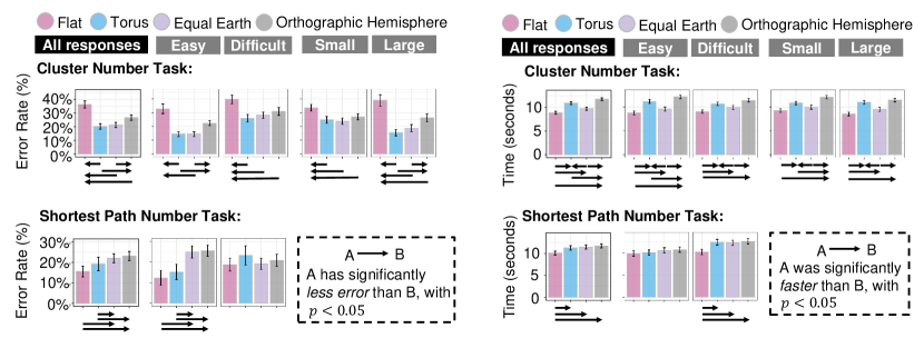
[]This diagram shows an the results of Study 2 in terms of error rate (left) and Time (right). Error bars are 95% confidence intervals. Significant differences between projections are shown as arrows.
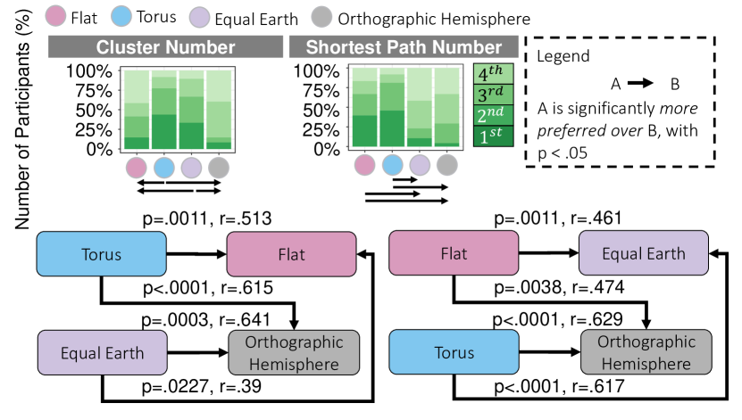
[Legend]This diagram shows user confidence ranking of each condition for two tested tasks. Arrows indicate statistical significance with . Effect size results of Cohen’s r (Cohen, 2013) are presented along with the arrows.
6.8. Key Findings and Discussion
We report on the most significant findings for Cluster Number
![[Uncaptioned image]](/html/2202.10845/assets/x226.png) , Shortest Path Number
, Shortest Path Number
![[Uncaptioned image]](/html/2202.10845/assets/x227.png) visually in Figure 7 and Figure 8. Detailed statistical results and pairwise effect sizes are provided in Section A.2.
visually in Figure 7 and Figure 8. Detailed statistical results and pairwise effect sizes are provided in Section A.2.
For Cluster Number
![[Uncaptioned image]](/html/2202.10845/assets/x228.png) , Equal Earth
, Equal Earth
![[Uncaptioned image]](/html/2202.10845/assets/x229.png) and Torus
and Torus
![[Uncaptioned image]](/html/2202.10845/assets/x230.png) performed equally well and Equal Earth
performed equally well and Equal Earth
![[Uncaptioned image]](/html/2202.10845/assets/x231.png) was slightly faster than Torus
was slightly faster than Torus
![[Uncaptioned image]](/html/2202.10845/assets/x232.png) , while they both significantly outperformed Orthographic Hemisphere
, while they both significantly outperformed Orthographic Hemisphere
![[Uncaptioned image]](/html/2202.10845/assets/x233.png) in terms of Error, Time, and Rank.
The poor performance of Orthographic Hemisphere
in terms of Error, Time, and Rank.
The poor performance of Orthographic Hemisphere
![[Uncaptioned image]](/html/2202.10845/assets/x234.png) compared with Equal Earth
compared with Equal Earth
![[Uncaptioned image]](/html/2202.10845/assets/x235.png) and Torus
and Torus
![[Uncaptioned image]](/html/2202.10845/assets/x236.png) was found statistically significant with moderate and large effect sizes for Error (All, Easy, Large), Time (Easy, Large), and large effects for Rank (Figure 7-top, Figure 8, Section A.2: Figure 15, Figure 16, and Figure 17), confirming H2-1, H2-2 for (RQ1, RQ3).
Surprisingly, while results from Study 1 (Section 4.8) showed that interactive Orthographic Hemisphere
was found statistically significant with moderate and large effect sizes for Error (All, Easy, Large), Time (Easy, Large), and large effects for Rank (Figure 7-top, Figure 8, Section A.2: Figure 15, Figure 16, and Figure 17), confirming H2-1, H2-2 for (RQ1, RQ3).
Surprisingly, while results from Study 1 (Section 4.8) showed that interactive Orthographic Hemisphere
![[Uncaptioned image]](/html/2202.10845/assets/x237.png) tended to be more accurate than Equal Earth
tended to be more accurate than Equal Earth
![[Uncaptioned image]](/html/2202.10845/assets/x238.png) for distance comparisons and not worse than any other projections for area comparisons, it turned out to be significantly worse than Equal Earth
for distance comparisons and not worse than any other projections for area comparisons, it turned out to be significantly worse than Equal Earth
![[Uncaptioned image]](/html/2202.10845/assets/x239.png) and Torus
and Torus
![[Uncaptioned image]](/html/2202.10845/assets/x240.png) for reading Cluster Number
for reading Cluster Number
![[Uncaptioned image]](/html/2202.10845/assets/x241.png) .
.
While it has the advantage of being a straightforward mapping from the sphere, Orthographic Hemisphere
![[Uncaptioned image]](/html/2202.10845/assets/x242.png) is an interrupted and non-area-preserving projection. Therefore, we conjecture that this discontinuity caused participants to struggle to make out cluster boundaries as compared with continuous representations in Torus
is an interrupted and non-area-preserving projection. Therefore, we conjecture that this discontinuity caused participants to struggle to make out cluster boundaries as compared with continuous representations in Torus
![[Uncaptioned image]](/html/2202.10845/assets/x243.png) and Equal Earth
and Equal Earth
![[Uncaptioned image]](/html/2202.10845/assets/x244.png) . Furthermore, there is no link distortion in Torus
. Furthermore, there is no link distortion in Torus
![[Uncaptioned image]](/html/2202.10845/assets/x245.png) . This was supported by participants feedback, e.g., “The ‘Equal Earth’ method felt much easier to distinguish every [individual] cluster.” (P20), and “Orthographic Hemisphere uses 2 maps so it is much more difficult to interpret than the others […] making it harder to isolate clusters.” (P12). More quotes can be found in Section A.2.1.
. This was supported by participants feedback, e.g., “The ‘Equal Earth’ method felt much easier to distinguish every [individual] cluster.” (P20), and “Orthographic Hemisphere uses 2 maps so it is much more difficult to interpret than the others […] making it harder to isolate clusters.” (P12). More quotes can be found in Section A.2.1.
We also note that although being statistically significant, the small effect sizes indicate that Equal Earth
![[Uncaptioned image]](/html/2202.10845/assets/x246.png) is slightly faster than Torus
is slightly faster than Torus
![[Uncaptioned image]](/html/2202.10845/assets/x247.png) (Helske et al., 2021; Cockburn et al., 2020).
(Helske et al., 2021; Cockburn et al., 2020).
Equal Earth
![[Uncaptioned image]](/html/2202.10845/assets/x248.png) , Orthographic Hemisphere
, Orthographic Hemisphere
![[Uncaptioned image]](/html/2202.10845/assets/x249.png) and Torus
and Torus
![[Uncaptioned image]](/html/2202.10845/assets/x250.png) significantly resulted in less error than Flat
. Equal Earth
significantly resulted in less error than Flat
. Equal Earth
![[Uncaptioned image]](/html/2202.10845/assets/x251.png) and Torus
and Torus
![[Uncaptioned image]](/html/2202.10845/assets/x252.png) were significantly preferred over Flat
but Torus
were significantly preferred over Flat
but Torus
![[Uncaptioned image]](/html/2202.10845/assets/x253.png) and Orthographic Hemisphere
and Orthographic Hemisphere
![[Uncaptioned image]](/html/2202.10845/assets/x254.png) took longer time than Flat
.
This was found statistically significant with moderate and large effect sizes (Figure 7-top, Figure 8, Section A.2: Figure 15, Figure 16, and Figure 17), leading us to reject H2-1 for (RQ2) and confirm H2-2 for (RQ2). These results provide strong evidence that with automatic panning and interaction, participants were able to better identify the high-level network structures using spherical projections.
They also confirm Chen et al.’s results where toroidal layouts with automatic panning significantly outperformed Flat
in terms of error for cluster understanding tasks (Chen
et al., 2021a). Some participants explicitly mentioned that good separation of clusters in continuous surfaces such as Equal Earth
took longer time than Flat
.
This was found statistically significant with moderate and large effect sizes (Figure 7-top, Figure 8, Section A.2: Figure 15, Figure 16, and Figure 17), leading us to reject H2-1 for (RQ2) and confirm H2-2 for (RQ2). These results provide strong evidence that with automatic panning and interaction, participants were able to better identify the high-level network structures using spherical projections.
They also confirm Chen et al.’s results where toroidal layouts with automatic panning significantly outperformed Flat
in terms of error for cluster understanding tasks (Chen
et al., 2021a). Some participants explicitly mentioned that good separation of clusters in continuous surfaces such as Equal Earth
![[Uncaptioned image]](/html/2202.10845/assets/x255.png) and Torus
and Torus
![[Uncaptioned image]](/html/2202.10845/assets/x256.png) helped understanding (Section A.2.1).
helped understanding (Section A.2.1).
Participants also mentioned the automatic panning helped them “see” without the need to interact e.g., “[with Equal Earth
![[Uncaptioned image]](/html/2202.10845/assets/x257.png) ,] even though if we move the picture [it] is very hard to understand the clusters. [It] turned out to be easiest to find the clusters (by not moving the picture).” (P37).
,] even though if we move the picture [it] is very hard to understand the clusters. [It] turned out to be easiest to find the clusters (by not moving the picture).” (P37).
For Shortest Path Number
![[Uncaptioned image]](/html/2202.10845/assets/x258.png) , Flat
and Torus
, Flat
and Torus
![[Uncaptioned image]](/html/2202.10845/assets/x259.png) performed equally well, both significantly outperforming Equal Earth
performed equally well, both significantly outperforming Equal Earth
![[Uncaptioned image]](/html/2202.10845/assets/x260.png) and Orthographic Hemisphere
and Orthographic Hemisphere
![[Uncaptioned image]](/html/2202.10845/assets/x261.png) in terms of Error and Rank, while Flat
is faster than all representations. We found Flat
and Torus
in terms of Error and Rank, while Flat
is faster than all representations. We found Flat
and Torus
![[Uncaptioned image]](/html/2202.10845/assets/x262.png) have a lower error rate than Equal Earth
have a lower error rate than Equal Earth
![[Uncaptioned image]](/html/2202.10845/assets/x263.png) and Orthographic Hemisphere
and Orthographic Hemisphere
![[Uncaptioned image]](/html/2202.10845/assets/x264.png) for all responses (moderate effects) and Easy (large effects) (Figure 7-bottom, Section A.2: Figure 15 and Figure 16). There is a strong evidence that Torus
for all responses (moderate effects) and Easy (large effects) (Figure 7-bottom, Section A.2: Figure 15 and Figure 16). There is a strong evidence that Torus
![[Uncaptioned image]](/html/2202.10845/assets/x265.png) is more preferred (large effects) over Equal Earth
is more preferred (large effects) over Equal Earth
![[Uncaptioned image]](/html/2202.10845/assets/x266.png) and Orthographic Hemisphere
and Orthographic Hemisphere
![[Uncaptioned image]](/html/2202.10845/assets/x267.png) , while Flat
is more preferred (moderate effects) over Equal Earth
, while Flat
is more preferred (moderate effects) over Equal Earth
![[Uncaptioned image]](/html/2202.10845/assets/x268.png) and Orthographic Hemisphere
and Orthographic Hemisphere
![[Uncaptioned image]](/html/2202.10845/assets/x269.png) (Figure 8 and Section A.2: Figure 17). Flat
was the fastest for All Responses (small and moderate effects) and Hard (moderate and large effects). We therefore accept H2-3, H2-4 for (RQ3) but reject H2-3, H2-4 for Flat
.
(Figure 8 and Section A.2: Figure 17). Flat
was the fastest for All Responses (small and moderate effects) and Hard (moderate and large effects). We therefore accept H2-3, H2-4 for (RQ3) but reject H2-3, H2-4 for Flat
.
We conjecture that although Torus
![[Uncaptioned image]](/html/2202.10845/assets/x270.png) involves broken links across the boundaries, it appears similar to Flat
using straight links
while the distortion of paths in Equal Earth
involves broken links across the boundaries, it appears similar to Flat
using straight links
while the distortion of paths in Equal Earth
![[Uncaptioned image]](/html/2202.10845/assets/x271.png) might hamper path tracing tasks, as participants mentioned “Flat surface is easier to read, it helps sometimes when you can also move it. Earth-like is just hard to use, especially when it’s an equal globe.” (P9), and “the warping in [Equal Earth
might hamper path tracing tasks, as participants mentioned “Flat surface is easier to read, it helps sometimes when you can also move it. Earth-like is just hard to use, especially when it’s an equal globe.” (P9), and “the warping in [Equal Earth
![[Uncaptioned image]](/html/2202.10845/assets/x272.png) ] made my eyes hurt a little therefore its in 4th place, and the torus being the most straight forward gets 1st with [Flat
] in second as they’re very similar.” (P13). On the other hand, Orthographic Hemisphere
] made my eyes hurt a little therefore its in 4th place, and the torus being the most straight forward gets 1st with [Flat
] in second as they’re very similar.” (P13). On the other hand, Orthographic Hemisphere
![[Uncaptioned image]](/html/2202.10845/assets/x273.png) has less link distortion but the interruption between two hemispheres and the strong perspective distortion near the boundary of the maps may make participants confused, supported by participants’ feedback (Section A.2.1).
has less link distortion but the interruption between two hemispheres and the strong perspective distortion near the boundary of the maps may make participants confused, supported by participants’ feedback (Section A.2.1).
Although automatic panning (Section 5.2) provides some benefits for reducing split of clusters across the boundaries for Cluster Number
![[Uncaptioned image]](/html/2202.10845/assets/x274.png) , it seems it has less benefits for Shortest Path Number
, it seems it has less benefits for Shortest Path Number
![[Uncaptioned image]](/html/2202.10845/assets/x275.png) , as participants mentioned they still need to position the image to see the full path to identify the shortest path connecting the nodes within the time limit (Section A.2.1).
, as participants mentioned they still need to position the image to see the full path to identify the shortest path connecting the nodes within the time limit (Section A.2.1).
Overall, these findings suggest that Torus
![[Uncaptioned image]](/html/2202.10845/assets/x276.png) presents a general solution being not only less error prone than Flat
or Orthographic Hemisphere
presents a general solution being not only less error prone than Flat
or Orthographic Hemisphere
![[Uncaptioned image]](/html/2202.10845/assets/x277.png) for Cluster Number
for Cluster Number
![[Uncaptioned image]](/html/2202.10845/assets/x278.png) , but also comparable to Flat
for Shortest Path Number
, but also comparable to Flat
for Shortest Path Number
![[Uncaptioned image]](/html/2202.10845/assets/x279.png) .
.
6.9. Limitations
A limitation of our study is that we only tested with one layout algorithm. While many different algorithms exist for Flat
and it is possible that other layout algorithms could be adapted to spherical and torus embeddings, doing so is not necessarily trivial.
Also, it should be noted that there are algorithms which can optimise layout for a known set of clusters (i.e. where the cluster labelling is known in advance) (Meulemans et al., 2013; Collins
et al., 2009; Gansner
et al., 2009; Hu
et al., 2010). However, for the tasks tested in this paper we do not preidentify the clusters but rather leave cluster identification as the user task.
Similar layouts (Dwyer
et al., 2008) have been used before for cluster understanding tasks on torus layouts (Chen
et al., 2020, 2021a).
7. Conclusion and Future Work
The overwhelming finding in Study 1 that interactive panning led to significantly lower error rate and more preferred over standard map projections across all tasks tested suggests that such panning should be routinely provided in online world maps, for example in education or in reporting of world events, climate patterns, and so on. While less clear, our results indicated that Equal Earth
![[Uncaptioned image]](/html/2202.10845/assets/x280.png) was the best performing continuous projection, while the straight-forward Orthographic Hemisphere
was the best performing continuous projection, while the straight-forward Orthographic Hemisphere
![[Uncaptioned image]](/html/2202.10845/assets/x281.png) was an effective hemispheric projection. Our results also indicate that even with interaction, Equirectangular
was an effective hemispheric projection. Our results also indicate that even with interaction, Equirectangular
![[Uncaptioned image]](/html/2202.10845/assets/x282.png) may be a poor choice for comparing areas and estimating directions.
may be a poor choice for comparing areas and estimating directions.
Our Study 2 results also confirm the benefits of topologically closed surfaces, such as the surface of a torus or sphere, when using node-link diagrams to investigate network structure. All of Equal Earth
![[Uncaptioned image]](/html/2202.10845/assets/x283.png) , Orthographic Hemisphere
, Orthographic Hemisphere
![[Uncaptioned image]](/html/2202.10845/assets/x284.png) , and Torus
, and Torus
![[Uncaptioned image]](/html/2202.10845/assets/x285.png) outperformed Flat
for cluster understanding tasks. While the spherical projections impeded path following tasks, it seems Torus
outperformed Flat
for cluster understanding tasks. While the spherical projections impeded path following tasks, it seems Torus
![[Uncaptioned image]](/html/2202.10845/assets/x286.png) may be a good general solution, being as accurate as Flat
for path following.
Although they have been explored in research, 2D projections of toroidal and spherical network layouts are rarely seen in practice. This may be because until recently effective layout and projection methods for such geometries were not easily available. We intend to make all our algorithms and extensions of existing open-source tools available for easy consumption in web applications via GitHub and npm packages.
may be a good general solution, being as accurate as Flat
for path following.
Although they have been explored in research, 2D projections of toroidal and spherical network layouts are rarely seen in practice. This may be because until recently effective layout and projection methods for such geometries were not easily available. We intend to make all our algorithms and extensions of existing open-source tools available for easy consumption in web applications via GitHub and npm packages.
A limitation of our work is that there are many more spherical map projections than those evaluated here, although we tried to select the most representative techniques. Further work may extend such evaluation to other projection types. Another interesting topic for future investigation would be investigating spherical and torus projections of other types of abstract data representation, such as multi-dimensional scaling techniques of high-dimensional data. Another family of interactive techniques for exploring graphs involve applying spatial distortion around regions of interest to achieve a kind of “structure aware zooming”, e.g. (Wang et al., 2018). It would be interesting to compare the efficacy of these techniques against interactive sphere and torus projections.
Acknowledgements.
We thank Bernhard Jenny, Lonni Besançon, Sarah Schöttler, Hong Gui, Mengxing Li, Ishwari Bhade, Umair Afzal, Sunny Singh for helpful discussion about the study design, anonymous participants for user study feedback, and our reviewers for helpful suggestions to improve this manuscript. We thank Stay Healthy and Monash eSolution crew for their technical support. This research is supported in part by Monash FIT Graduate Research Candidature Funding Scheme.References
- (1)
- Bach et al. (2015) Benjamin Bach, Conglei Shi, Nicolas Heulot, Tara Madhyastha, Tom Grabowski, and Pierre Dragicevic. 2015. Time curves: Folding time to visualize patterns of temporal evolution in data. IEEE transactions on visualization and computer graphics 22, 1 (2015), 559–568.
- Barabási and Albert (1999) Albert-László Barabási and Réka Albert. 1999. Emergence of scaling in random networks. science 286, 5439 (1999), 509–512.
- Bates et al. (2015) Douglas Bates, Martin Mächler, Ben Bolker, and Steve Walker. 2015. Fitting Linear Mixed-Effects Models Using lme4. Journal of Statistical Software 67, 1 (2015), 47 pages. https://doi.org/10.18637/jss.v067.i01
- Besançon et al. (2017) Lonni Besançon, Mehdi Ammi, and Tobias Isenberg. 2017. Pressure-based gain factor control for mobile 3D interaction using locally-coupled devices. In Proceedings of the 2017 CHI Conference on Human Factors in Computing Systems. 1831–1842.
- Besançon et al. (2017) Lonni Besançon, Paul Issartel, Mehdi Ammi, and Tobias Isenberg. 2017. Mouse, Tactile, and Tangible Input for 3D Manipulation. In Proceedings of the ACM Conference on Human Factors in Computing Systems (CHI). Denver, United States, 4727–4740. https://doi.org/10.1145/3025453.3025863
- Bostock and Davies (2013) Michael Bostock and Jason Davies. 2013. Code as Cartography. The Cartographic Journal 50, 2 (May 2013), 129–135. https://doi.org/10.1179/0008704113Z.00000000078
- Brandes et al. (2003) Ulrik Brandes, Marco Gaertler, and Dorothea Wagner. 2003. Experiments on graph clustering algorithms. In European Symposium on Algorithms. Springer, 568–579.
- Brath and MacMurchy (2012) Richard Brath and Peter MacMurchy. 2012. Sphere-based information visualization: Challenges and benefits. In 2012 16th International Conference on Information Visualisation. IEEE, 1–6.
- Brehmer et al. (2018) Matthew Brehmer, Bongshin Lee, Petra Isenberg, and Eun Kyoung Choe. 2018. Visualizing ranges over time on mobile phones: a task-based crowdsourced evaluation. IEEE transactions on visualization and computer graphics 25, 1 (2018), 619–629.
- Carbon (2010) Claus-Christian Carbon. 2010. The Earth is flat when personally significant experiences with the sphericity of the Earth are absent. Cognition 116, 1 (2010), 130–135.
- Chen et al. (2021a) Kun-Ting Chen, Tim Dwyer, Benjamin Bach, and Kim Marriott. 2021a. It’s a Wrap: Toroidal Wrapping of Network Visualisations Supports Cluster Understanding Tasks. In Proceedings of the 2021 CHI Conference on Human Factors in Computing Systems. 1–12.
- Chen et al. (2021b) Kun-Ting Chen, Tim Dwyer, Benjamin Bach, and Kim Marriott. 2021b. Rotate or Wrap? Interactive Visualisations of Cyclical Data on Cylindrical or Toroidal Topologies. IEEE Transactions on Visualization and Computer Graphics 28, 1 (2021), 727–736.
- Chen et al. (2020) Kun-Ting Chen, Tim Dwyer, Kim Marriott, and Benjamin Bach. 2020. DoughNets: Visualising Networks Using Torus Wrapping. In Proceedings of the 2020 CHI Conference on Human Factors in Computing Systems. 1–11.
- Cockburn et al. (2020) Andy Cockburn, Pierre Dragicevic, Lonni Besançon, and Carl Gutwin. 2020. Threats of a replication crisis in empirical computer science. Commun. ACM 63, 8 (2020), 70–79.
- Cohen (2013) Jacob Cohen. 2013. Statistical power analysis for the behavioral sciences. Academic press.
- Collins et al. (2009) Christopher Collins, Gerald Penn, and Sheelagh Carpendale. 2009. Bubble sets: Revealing set relations with isocontours over existing visualizations. IEEE Transactions on Visualization and Computer Graphics 15, 6 (2009), 1009–1016.
- Davies (2013) Jason Davies. 2013. Rotate the World. https://www.jasondavies.com/maps/rotate/
- De Leeuw and Mair (2009) Jan De Leeuw and Patrick Mair. 2009. Multidimensional scaling using majorization: SMACOF in R. Journal of statistical software 31, 1 (2009), 1–30.
- Du et al. (2017) Fan Du, Nan Cao, Yu-Ru Lin, Panpan Xu, and Hanghang Tong. 2017. isphere: Focus+ context sphere visualization for interactive large graph exploration. In Proceedings of the 2017 CHI Conference on Human Factors in Computing Systems. 2916–2927.
- Dwyer et al. (2008) Tim Dwyer, Kim Marriott, and Michael Wybrow. 2008. Topology preserving constrained graph layout. In International Symposium on Graph Drawing. Springer, 230–241.
- Fortunato (2010) Santo Fortunato. 2010. Community detection in graphs. Physics reports 486, 3-5 (2010), 75–174.
- Gansner et al. (2009) Emden R Gansner, Yifan Hu, and Stephen G Kobourov. 2009. Gmap: Drawing graphs as maps. In International Symposium on Graph Drawing. Springer, 405–407.
- Gansner et al. (2004) Emden R Gansner, Yehuda Koren, and Stephen North. 2004. Graph drawing by stress majorization. In International Symposium on Graph Drawing. Springer, 239–250.
- Greffard et al. (2011) Nicolas Greffard, Fabien Picarougne, and Pascale Kuntz. 2011. Visual community detection: An evaluation of 2d, 3d perspective and 3d stereoscopic displays. In International Symposium on Graph Drawing. Springer, 215–225.
- Helske et al. (2021) Jouni Helske, Satu Helske, Matthew Cooper, Anders Ynnerman, and Lonni Besancon. 2021. Can visualization alleviate dichotomous thinking Effects of visual representations on the cliff effect. IEEE Transactions on Visualization and Computer Graphics (2021).
- Hennerdal (2015) Pontus Hennerdal. 2015. Beyond the periphery: Child and adult understanding of world map continuity. Annals of the Association of American Geographers 105, 4 (2015), 773–790.
- Herman et al. (2018) Lukáš Herman, Vojtěch Juřík, Zdeněk Stachoň, Daniel Vrbík, Jan Russnák, and Tomáš Řezník. 2018. Evaluation of user performance in interactive and static 3D maps. ISPRS International Journal of Geo-Information 7, 11 (2018), 415.
- Hruby et al. (2016) Florian Hruby, Mónica Chico Avelino, and Raymundo Montoya Ayala. 2016. Journey to the end of the world Map–How edges of world maps shape the spatial mind. Journal for Geographic Information Science 1 (2016), 314–323.
- Hu et al. (2010) Yifan Hu, Emden R Gansner, and Stephen Kobourov. 2010. Visualizing graphs and clusters as maps. IEEE Computer Graphics and Applications 30, 6 (2010), 54–66.
- Huang et al. (2009) Weidong Huang, Peter Eades, and Seok-Hee Hong. 2009. Measuring effectiveness of graph visualizations: A cognitive load perspective. Information Visualization 8, 3 (2009), 139–152.
- in Human-Computer Interaction Working Group (2019) Transparent Statistics in Human-Computer Interaction Working Group. 2019. Transparent Statistics Guidelines. https://doi.org/10.5281/zenodo.1186169 (Available at https://transparentstats.github.io/guidelines).
- Jenny et al. (2016) Bernhard Jenny, Johannes Liem, Bojan Šavrič, and William M. Putman. 2016. Interactive video maps: A year in the life of Earth’s CO2. Journal of Maps 12, sup1 (Nov. 2016), 36–42. https://doi.org/10.1080/17445647.2016.1157323
- Jenny et al. (2017) Bernhard Jenny, Bojan Šavrič, Nicholas D Arnold, Brooke E Marston, and Charles A Preppernau. 2017. A guide to selecting map projections for world and hemisphere maps. In Choosing a map projection. Springer, 213–228.
- Kobourov and Landis (2008) Stephen G Kobourov and Matthew Landis. 2008. Morphing planar graphs in spherical space. (2008).
- Kobourov and Wampler (2005) Stephen G Kobourov and Kevin Wampler. 2005. Non-Euclidean spring embedders. IEEE Transactions on Visualization and Computer Graphics 11, 6 (2005), 757–767.
- Kwon et al. (2016) Oh-Hyun Kwon, Chris Muelder, Kyungwon Lee, and Kwan-Liu Ma. 2016. A study of layout, rendering, and interaction methods for immersive graph visualization. IEEE transactions on visualization and computer graphics 22, 7 (2016), 1802–1815.
- Lee et al. (2006) Bongshin Lee, Catherine Plaisant, Cynthia Sims Parr, Jean-Daniel Fekete, and Nathalie Henry. 2006. Task Taxonomy for Graph Visualization. In Proceedings of the 2006 AVI Workshop on BEyond Time and Errors: Novel Evaluation Methods for Information Visualization (Venice, Italy) (BELIV ’06). ACM, New York, NY, USA, 1–5. https://doi.org/10.1145/1168149.1168168
- Lenth (2016) Russell V. Lenth. 2016. Least-Squares Means: The R Package lsmeans. Journal of Statistical Software 69, 1 (2016), 33 pages. https://doi.org/10.18637/jss.v069.i01
- Manning (2017) Christopher Manning. 2017. Spherical Force-Directed Layout. http://bl.ocks.org/christophermanning/4208494
- Meulemans et al. (2013) Wouter Meulemans, Nathalie Henry Riche, Bettina Speckmann, Basak Alper, and Tim Dwyer. 2013. Kelpfusion: A hybrid set visualization technique. IEEE transactions on visualization and computer graphics 19, 11 (2013), 1846–1858.
- Munzner (2014) Tamara Munzner. 2014. Visualization analysis and design. CRC press.
- Newman (2006) Mark EJ Newman. 2006. Modularity and community structure in networks. Proceedings of the national academy of sciences 103, 23 (2006), 8577–8582.
- Okoe et al. (2018) Mershack Okoe, Radu Jianu, and Stephen Kobourov. 2018. Node-link or adjacency matrices: Old question, new insights. IEEE transactions on visualization and computer graphics 25, 10 (2018), 2940–2952.
- Palan and Schitter (2018) Stefan Palan and Christian Schitter. 2018. Prolific. ac—A subject pool for online experiments. Journal of Behavioral and Experimental Finance 17 (2018), 22–27.
- Pallant (2013) Julie Pallant. 2013. SPSS survival manual. McGraw-hill education (UK).
- Peer et al. (2017) Eyal Peer, Laura Brandimarte, Sonam Samat, and Alessandro Acquisti. 2017. Beyond the Turk: Alternative platforms for crowdsourcing behavioral research. Journal of Experimental Social Psychology 70 (2017), 153–163.
- Perry et al. (2020) Scott Perry, Mason Sun Yin, Kathryn Gray, and Stephen Kobourov. 2020. Drawing Graphs on the Sphere. In Proceedings of the International Conference on Advanced Visual Interfaces. 1–9.
- Purchase (2002) Helen C Purchase. 2002. Metrics for graph drawing aesthetics. Journal of Visual Languages & Computing 13, 5 (2002), 501–516.
- Rodighiero (2020) Dario Rodighiero. 2020. Drawing Network Visualizations on a Continuous, Spherical Surface. In 2020 24th International Conference Information Visualisation (IV). IEEE, 573–580.
- Saket et al. (2014) Bahador Saket, Paolo Simonetto, and Stephen Kobourov. 2014. Group-level graph visualization taxonomy. arXiv preprint arXiv:1403.7421 (2014).
- Satriadi et al. (2021) Kadek Ananta Satriadi, Barrett Ens, Tobias Czauderna, Maxime Cordeil, and Bernhard Jenny. 2021. Quantitative Data Visualisation on Virtual Globes. In Proceedings of the 2021 CHI Conference on Human Factors in Computing Systems. 1–14.
- Šavric et al. (2015) Bojan Šavric, Bernhard Jenny, Denis White, and Daniel R Strebe. 2015. User preferences for world map projections. Cartography and Geographic Information Science 42, 5 (2015), 398–409.
- Šavrič et al. (2019) Bojan Šavrič, Tom Patterson, and Bernhard Jenny. 2019. The equal earth map projection. International Journal of Geographical Information Science 33, 3 (2019), 454–465.
- Schäfer and Schwarz (2019) Thomas Schäfer and Marcus A Schwarz. 2019. The meaningfulness of effect sizes in psychological research: Differences between sub-disciplines and the impact of potential biases. Frontiers in Psychology 10 (2019), 813.
- Schöttler et al. (2021) Sarah Schöttler, Yalong Yang, Hanspeter Pfister, and Benjamin Bach. 2021. Visualizing and interacting with geospatial networks: A survey and design space. In Computer Graphics Forum. Wiley Online Library.
- Snyder (1987) John Parr Snyder. 1987. Map projections–A working manual. Vol. 1395. US Government Printing Office.
- Snyder (1997) John P Snyder. 1997. Flattening the earth: two thousand years of map projections. University of Chicago Press.
- Wang et al. (2018) Yunhai Wang, Yanyan Wang, Haifeng Zhang, Yinqi Sun, Chi-Wing Fu, Michael Sedlmair, Baoquan Chen, and Oliver Deussen. 2018. Structure-aware fisheye views for efficient large graph exploration. IEEE transactions on visualization and computer graphics 25, 1 (2018), 566–575.
- Ware and Mitchell (2008) Colin Ware and Peter Mitchell. 2008. Visualizing graphs in three dimensions. ACM Transactions on Applied Perception (TAP) 5, 1 (2008), 1–15.
- Watts and Strogatz (1998) Duncan J Watts and Steven H Strogatz. 1998. Collective dynamics of ‘small-world’networks. nature 393, 6684 (1998), 440–442.
- Williams (1949) Evan James Williams. 1949. Experimental designs balanced for the estimation of residual effects of treatments. Australian Journal of Chemistry 2, 2 (1949), 149–168.
- Wu and Takatsuka (2006) Yingxin Wu and Masahiro Takatsuka. 2006. Spherical self-organizing map using efficient indexed geodesic data structure. Neural Networks 19, 6-7 (2006), 900–910.
- Xu et al. (2012) Kai Xu, Chris Rooney, Peter Passmore, Dong-Han Ham, and Phong H Nguyen. 2012. A user study on curved edges in graph visualization. IEEE transactions on visualization and computer graphics 18, 12 (2012), 2449–2456.
- Yang et al. (2019) Yalong Yang, Tim Dwyer, Bernhard Jenny, Kim Marriott, Maxime Cordeil, and Haohui Chen. 2019. Origin-Destination Flow Maps in Immersive Environments. IEEE Transactions on Visualization and Computer Graphics 25, 1 (2019), 693–703. https://doi.org/10.1109/tvcg.2018.2865192
- Yang et al. (2018) Yalong Yang, Bernhard Jenny, Tim Dwyer, Kim Marriott, Haohui Chen, and Maxime Cordeil. 2018. Maps and globes in virtual reality. In Computer Graphics Forum, Vol. 37. Wiley Online Library, 427–438.
- Yoghourdjian et al. (2020) Vahan Yoghourdjian, Yalong Yang, Tim Dwyer, Lee Lawrence, Michael Wybrow, and Kim Marriott. 2020. Scalability of network visualisation from a cognitive load perspective. IEEE Transactions on Visualization and Computer Graphics 27, 2 (2020), 1677–1687.
- Zheng et al. (2018) Jonathan X Zheng, Samraat Pawar, and Dan FM Goodman. 2018. Graph drawing by stochastic gradient descent. IEEE transactions on visualization and computer graphics 25, 9 (2018), 2738–2748.
Appendix A Study Results
In the following, significance values are reported for , , and , respectively, abbreviated by the number of stars in parenthesis.
A.1. Study 1: Map Projection Readability
For Distance Comparison
![[Uncaptioned image]](/html/2202.10845/assets/x287.png) , we found Interaction () and Map Projection Difficulty () both had a significant effect on Time. For Interaction, posthoc analysis shows that
Static was faster than Interactive ().
For Map Projection Difficulty, posthoc analysis shows that in Easy, Equirectangular
, we found Interaction () and Map Projection Difficulty () both had a significant effect on Time. For Interaction, posthoc analysis shows that
Static was faster than Interactive ().
For Map Projection Difficulty, posthoc analysis shows that in Easy, Equirectangular
![[Uncaptioned image]](/html/2202.10845/assets/x288.png) and Equal Earth
and Equal Earth
![[Uncaptioned image]](/html/2202.10845/assets/x289.png) were faster than Orthographic Hemisphere
were faster than Orthographic Hemisphere
![[Uncaptioned image]](/html/2202.10845/assets/x290.png) () and Mollweide Hemisphere
() and Mollweide Hemisphere
![[Uncaptioned image]](/html/2202.10845/assets/x291.png) (). Hammer
(). Hammer
![[Uncaptioned image]](/html/2202.10845/assets/x292.png) was also faster than Mollweide Hemisphere
was also faster than Mollweide Hemisphere
![[Uncaptioned image]](/html/2202.10845/assets/x293.png) (). In Hard, Equal Earth
(). In Hard, Equal Earth
![[Uncaptioned image]](/html/2202.10845/assets/x294.png) was faster than Orthographic Hemisphere
was faster than Orthographic Hemisphere
![[Uncaptioned image]](/html/2202.10845/assets/x295.png) () and Mollweide Hemisphere
() and Mollweide Hemisphere
![[Uncaptioned image]](/html/2202.10845/assets/x296.png) ().
().
We found Map Projection had a significant effect on error rate in Hard (). Orthographic Hemisphere
![[Uncaptioned image]](/html/2202.10845/assets/x297.png) was more accurate than Equal Earth
was more accurate than Equal Earth
![[Uncaptioned image]](/html/2202.10845/assets/x298.png) () and Hammer
() and Hammer
![[Uncaptioned image]](/html/2202.10845/assets/x299.png) (). We also found Interactive was more accurate than Static in all Map Projection ().
(). We also found Interactive was more accurate than Static in all Map Projection ().
In Static Map Projection, participants preferred Equal Earth
![[Uncaptioned image]](/html/2202.10845/assets/x300.png) over Hammer
over Hammer
![[Uncaptioned image]](/html/2202.10845/assets/x301.png) (), Mollweide Hemisphere
(), Mollweide Hemisphere
![[Uncaptioned image]](/html/2202.10845/assets/x302.png) (), and Orthographic Hemisphere
(), and Orthographic Hemisphere
![[Uncaptioned image]](/html/2202.10845/assets/x303.png) ().
().
For Area Comparison
![[Uncaptioned image]](/html/2202.10845/assets/x304.png) , we found Interaction (), Map Projection Difficulty () and Map Projection Interaction () had a significant effect on time. For Area Comparison
, we found Interaction (), Map Projection Difficulty () and Map Projection Interaction () had a significant effect on time. For Area Comparison
![[Uncaptioned image]](/html/2202.10845/assets/x305.png) , Static was faster than Interactive (). For Map Projection Interaction (), Interactive Equal Earth
, Static was faster than Interactive (). For Map Projection Interaction (), Interactive Equal Earth
![[Uncaptioned image]](/html/2202.10845/assets/x306.png) was faster than Interactive Hammer
was faster than Interactive Hammer
![[Uncaptioned image]](/html/2202.10845/assets/x307.png) ().
().
We found Map Projection had a significant effect on Error in Interactive (), Easy Static () and Hard Interactive (). Mollweide Hemisphere
![[Uncaptioned image]](/html/2202.10845/assets/x308.png) was more accurate than Equirectangular
was more accurate than Equirectangular
![[Uncaptioned image]](/html/2202.10845/assets/x309.png) ().
Static Equal Earth
().
Static Equal Earth
![[Uncaptioned image]](/html/2202.10845/assets/x310.png) () and StaticMollweide Hemisphere
() and StaticMollweide Hemisphere
![[Uncaptioned image]](/html/2202.10845/assets/x311.png) () were more accurate than Static Equirectangular
() were more accurate than Static Equirectangular
![[Uncaptioned image]](/html/2202.10845/assets/x312.png) in Easy.
Interactive Mollweide Hemisphere
in Easy.
Interactive Mollweide Hemisphere
![[Uncaptioned image]](/html/2202.10845/assets/x313.png) and Interactive Interactive tended to be more accurate than Interactive Equirectangular
and Interactive Interactive tended to be more accurate than Interactive Equirectangular
![[Uncaptioned image]](/html/2202.10845/assets/x314.png) , but not statistically significant (with respectively).
We also found Interactive was more accurate than Static in all Map Projection (all ).
, but not statistically significant (with respectively).
We also found Interactive was more accurate than Static in all Map Projection (all ).
In Static Map Projection, participants preferred Equirectangular
![[Uncaptioned image]](/html/2202.10845/assets/x315.png) (), Equal Earth
(), Equal Earth
![[Uncaptioned image]](/html/2202.10845/assets/x316.png) () and Orthographic Hemisphere
() and Orthographic Hemisphere
![[Uncaptioned image]](/html/2202.10845/assets/x317.png) () than Hammer
() than Hammer
![[Uncaptioned image]](/html/2202.10845/assets/x318.png) .
.
For Direction estimation
![[Uncaptioned image]](/html/2202.10845/assets/x319.png) , we found Map Projection (), Interaction () and Map Projection Interaction () had a significant effect on time. For Direction estimation
, we found Map Projection (), Interaction () and Map Projection Interaction () had a significant effect on time. For Direction estimation
![[Uncaptioned image]](/html/2202.10845/assets/x320.png) , Static was faster than Interactive ().
In Static Map Projection, Equirectangular
, Static was faster than Interactive ().
In Static Map Projection, Equirectangular
![[Uncaptioned image]](/html/2202.10845/assets/x321.png) and Equal Earth
and Equal Earth
![[Uncaptioned image]](/html/2202.10845/assets/x322.png) were faster than Mollweide Hemisphere
were faster than Mollweide Hemisphere
![[Uncaptioned image]](/html/2202.10845/assets/x323.png) and Orthographic Hemisphere
and Orthographic Hemisphere
![[Uncaptioned image]](/html/2202.10845/assets/x324.png) (all ).
In Interactive Map Projection, Equal Earth
(all ).
In Interactive Map Projection, Equal Earth
![[Uncaptioned image]](/html/2202.10845/assets/x325.png) was faster than Mollweide Hemisphere
was faster than Mollweide Hemisphere
![[Uncaptioned image]](/html/2202.10845/assets/x326.png) ().
().
We found Map Projection had a significant effect on error rate in Interactive. Orthographic Hemisphere
![[Uncaptioned image]](/html/2202.10845/assets/x327.png) was more accurate than Equirectangular
was more accurate than Equirectangular
![[Uncaptioned image]](/html/2202.10845/assets/x328.png) (). We also found Interactive was more accurate than Static in all Map Projection ().
(). We also found Interactive was more accurate than Static in all Map Projection ().
We did not find significant difference in preference for Interactive groups.
A.1.1. Qualitative Feedback
In continuous projections, Equal Earth
![[Uncaptioned image]](/html/2202.10845/assets/x329.png) performed well in terms of Error for Area Comparison
performed well in terms of Error for Area Comparison
![[Uncaptioned image]](/html/2202.10845/assets/x330.png) , Time for Area Comparison
, Time for Area Comparison
![[Uncaptioned image]](/html/2202.10845/assets/x331.png) and Direction estimation
and Direction estimation
![[Uncaptioned image]](/html/2202.10845/assets/x332.png) , and Rank-Static for both Distance Comparison
, and Rank-Static for both Distance Comparison
![[Uncaptioned image]](/html/2202.10845/assets/x333.png) and Area Comparison
and Area Comparison
![[Uncaptioned image]](/html/2202.10845/assets/x334.png) . Equal Earth
. Equal Earth
![[Uncaptioned image]](/html/2202.10845/assets/x335.png) was not significantly worse than any other continuous projections.
The preference of Static Equal Earth
was not significantly worse than any other continuous projections.
The preference of Static Equal Earth
![[Uncaptioned image]](/html/2202.10845/assets/x336.png) was supported by our participants’ feedback, as they mentioned “I didn’t feel comfortable when the hemispheres were split into two separate circle portions. I preferred [equal earth] when they were a continuous map surface.” (P18, Distance-Static), and “the map’s edges [in equal earth projection] didn’t feel as distorted as other maps such as equirectangular.” (P23, Area-Static.) We also identified many positive comments for Equal Earth
was supported by our participants’ feedback, as they mentioned “I didn’t feel comfortable when the hemispheres were split into two separate circle portions. I preferred [equal earth] when they were a continuous map surface.” (P18, Distance-Static), and “the map’s edges [in equal earth projection] didn’t feel as distorted as other maps such as equirectangular.” (P23, Area-Static.) We also identified many positive comments for Equal Earth
![[Uncaptioned image]](/html/2202.10845/assets/x337.png) , e.g., “[equal earth projection] gave me a better sense of global spatial reasoning” (P34, Distance-Static), and “the equal earth projection was the easiest to visualise as it seemed to have a good balance of not being too distorted without having the difficulty of wrap around visualisations that the hemisphere projections had.” (P37, Distance-Static).
, e.g., “[equal earth projection] gave me a better sense of global spatial reasoning” (P34, Distance-Static), and “the equal earth projection was the easiest to visualise as it seemed to have a good balance of not being too distorted without having the difficulty of wrap around visualisations that the hemisphere projections had.” (P37, Distance-Static).
Participants disliked Hammer
![[Uncaptioned image]](/html/2202.10845/assets/x338.png) for Static-Area. For example, participants mentioned “I think [equirectangular] felt easier to read my first choice vs what I rate number 5 [for hammer].” (P17, Area-Static) and “the hammer too oval to make sense of.” (P19, Direction-Static).
for Static-Area. For example, participants mentioned “I think [equirectangular] felt easier to read my first choice vs what I rate number 5 [for hammer].” (P17, Area-Static) and “the hammer too oval to make sense of.” (P19, Direction-Static).
In hemispheric projections, interaction reduced Error of Orthographic Hemisphere
![[Uncaptioned image]](/html/2202.10845/assets/x339.png) to a point that it tended to have a lower error rate than some interactive continuous projections for Distance-Hard and Direction, and not significantly slower than any interactive projections across all tasks.
Orthographic Hemisphere
to a point that it tended to have a lower error rate than some interactive continuous projections for Distance-Hard and Direction, and not significantly slower than any interactive projections across all tasks.
Orthographic Hemisphere
![[Uncaptioned image]](/html/2202.10845/assets/x340.png) was perceived as less distorted than the other projections due to the “natural” orthographic distortion, which is similar to viewing the sphere at infinite distance (e.g. as if through a telescope). Furthermore, despite being hemispheric, Mollweide Hemisphere
was perceived as less distorted than the other projections due to the “natural” orthographic distortion, which is similar to viewing the sphere at infinite distance (e.g. as if through a telescope). Furthermore, despite being hemispheric, Mollweide Hemisphere
![[Uncaptioned image]](/html/2202.10845/assets/x341.png) , was found to be less intuitive for some tasks by participants. We conjecture that there is a slight distortion near the edge of two circles which may make it confusing when centring the region of interest, as participants mentioned “Orthographic hemisphere felt the easiest to compare because it was like looking at a globe, but the strange way of moving the mollewide hemisphere made it confusing, that is why that is my last option.” (P23, Area-Interactive), “The mollweide was a bit difficult to drag and place arrow.” (P23, Direction-Interactive.), and “Orthographic Hemisphere seemed the most accurate to me. The round shape was really useful. The Mollweide Hemisphere was tricky, I didn’t like the way the two points had to be on the separate circles for it to be accurate sometimes.” (P4, Direction-Interactive).
, was found to be less intuitive for some tasks by participants. We conjecture that there is a slight distortion near the edge of two circles which may make it confusing when centring the region of interest, as participants mentioned “Orthographic hemisphere felt the easiest to compare because it was like looking at a globe, but the strange way of moving the mollewide hemisphere made it confusing, that is why that is my last option.” (P23, Area-Interactive), “The mollweide was a bit difficult to drag and place arrow.” (P23, Direction-Interactive.), and “Orthographic Hemisphere seemed the most accurate to me. The round shape was really useful. The Mollweide Hemisphere was tricky, I didn’t like the way the two points had to be on the separate circles for it to be accurate sometimes.” (P4, Direction-Interactive).
However, there were also participants who did not like the hemisphere projections due to the need to inspect two separated spheres and instead they preferred non-hemisphere, e.g., “I found it a lot easier to identify on the single maps rather than the double because sometimes they were spaced too far away” (P11, Area-Interactive), “it was hard to picture how Mollweide and Orthographic Hemispheres connected.” (P7, Distance-Static), and “the map layout was easier to see because the targets were all on one map rather than two spheres.” (P36, Distance-Interactive).
Meanwhile, it seems many people were good at mentally connecting both hemispheres: “I found it easier to create comparisons that didn’t have a lot of distortion with the option of having the two side-by-side globes.” (P18, Direction-Interactive).
Even with interaction, Equirectangular
![[Uncaptioned image]](/html/2202.10845/assets/x342.png) still tended to perform poorly in terms of Error for Area Comparison
still tended to perform poorly in terms of Error for Area Comparison
![[Uncaptioned image]](/html/2202.10845/assets/x343.png) and Direction estimation
and Direction estimation
![[Uncaptioned image]](/html/2202.10845/assets/x344.png) .
Interactive Equirectangular
.
Interactive Equirectangular
![[Uncaptioned image]](/html/2202.10845/assets/x345.png) was still found to have a greater distortion near the poles than other projections, as participants mentioned “The sphere is easiest to visualize in my head, I was thinking about just drawing a line on a ball or other spherical shape. The ones with the biggest distortment on the edges confused me most.” (P13, Direction-Interactive) and “The Mollweide Hemisphere and Orthographic Hemisphere- easier to see a side by side comparison of the areas. The Hammer- less areas of distortion compared to the Equal Earth and Equirectangular. Equal Earth had too much distortion as did the Equirectangular which in my opinion distorted the most.” (P21, Area-Interactive).
was still found to have a greater distortion near the poles than other projections, as participants mentioned “The sphere is easiest to visualize in my head, I was thinking about just drawing a line on a ball or other spherical shape. The ones with the biggest distortment on the edges confused me most.” (P13, Direction-Interactive) and “The Mollweide Hemisphere and Orthographic Hemisphere- easier to see a side by side comparison of the areas. The Hammer- less areas of distortion compared to the Equal Earth and Equirectangular. Equal Earth had too much distortion as did the Equirectangular which in my opinion distorted the most.” (P21, Area-Interactive).
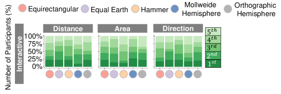 \Description
[Legend]
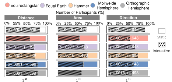 \Description
[Legend]
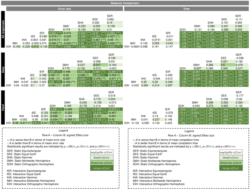
[]
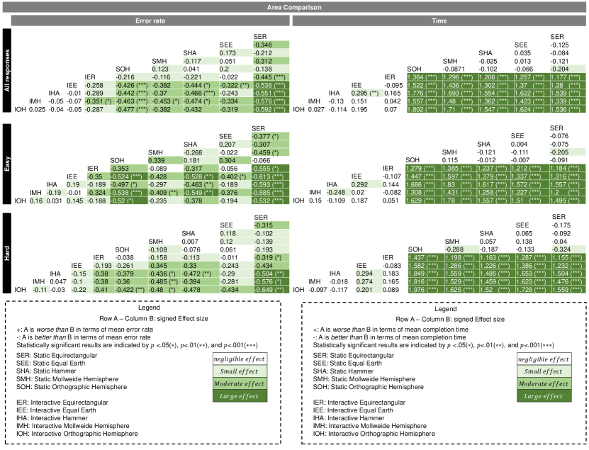
[]
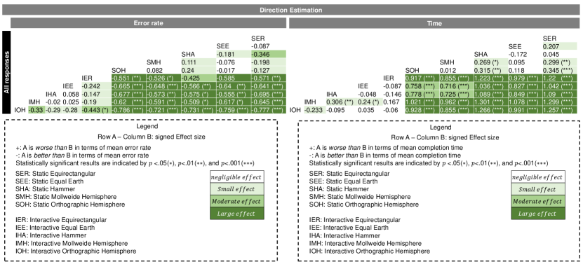
[]
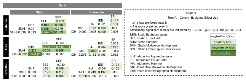
[Legend]
A.2. Study 2: Network Projection Readability
| Projections | Number of Graphs | Datasets | Number of Pixels | Crossing Counts | ||
|---|---|---|---|---|---|---|
| No Pan | Auto-Pan | No Pan | Auto-Pan | |||
Equal Earth
![[Uncaptioned image]](/html/2202.10845/assets/x352.png)
|
10 | Small+Easy, Small+Hard | 20916.3 | 23464.24 | N/A | N/A |
Orthographic Hemisphere
![[Uncaptioned image]](/html/2202.10845/assets/x353.png)
|
10 | Small+Easy, Small+Hard | N/A | N/A | 262.16 | 208.7 |
[Automatic panning results]Automatic panning reduces mean number of pixels at the boundary, number of edges crossing the boundaries compared with no panning for Small graphs at high (0.4) and low (0.3) modularity (with layout pre-computed by Algorithm 1);
For Cluster Number
![[Uncaptioned image]](/html/2202.10845/assets/x354.png) , we found Layout had a significant effect on error rate in All Responses (), Easy (), Hard (), Small (), and Large (). Torus
, we found Layout had a significant effect on error rate in All Responses (), Easy (), Hard (), Small (), and Large (). Torus
![[Uncaptioned image]](/html/2202.10845/assets/x355.png) (), Equal Earth
(), Equal Earth
![[Uncaptioned image]](/html/2202.10845/assets/x356.png) () and Orthographic Hemisphere
() and Orthographic Hemisphere
![[Uncaptioned image]](/html/2202.10845/assets/x357.png) () were more accurate than Flat
. Torus
() were more accurate than Flat
. Torus
![[Uncaptioned image]](/html/2202.10845/assets/x358.png) () and Equal Earth
() and Equal Earth
![[Uncaptioned image]](/html/2202.10845/assets/x359.png) () were more accurate than Orthographic Hemisphere
() were more accurate than Orthographic Hemisphere
![[Uncaptioned image]](/html/2202.10845/assets/x360.png) . We also found Torus
. We also found Torus
![[Uncaptioned image]](/html/2202.10845/assets/x361.png) and Equal Earth
and Equal Earth
![[Uncaptioned image]](/html/2202.10845/assets/x362.png) were more accurate than Flat
for Easy () and Orthographic Hemisphere
were more accurate than Flat
for Easy () and Orthographic Hemisphere
![[Uncaptioned image]](/html/2202.10845/assets/x363.png) for Easy (). We found Torus
for Easy (). We found Torus
![[Uncaptioned image]](/html/2202.10845/assets/x364.png) , Equal Earth
, Equal Earth
![[Uncaptioned image]](/html/2202.10845/assets/x365.png) , and Orthographic Hemisphere
, and Orthographic Hemisphere
![[Uncaptioned image]](/html/2202.10845/assets/x366.png) were more accurate than Flat
for Hard (), Small (). We also found Torus
were more accurate than Flat
for Hard (), Small (). We also found Torus
![[Uncaptioned image]](/html/2202.10845/assets/x367.png) (), Equal Earth
(), Equal Earth
![[Uncaptioned image]](/html/2202.10845/assets/x368.png) () and Orthographic Hemisphere
() and Orthographic Hemisphere
![[Uncaptioned image]](/html/2202.10845/assets/x369.png) () were more accurate than Flat
for Large. Torus
() were more accurate than Flat
for Large. Torus
![[Uncaptioned image]](/html/2202.10845/assets/x370.png) () and Equal Earth
() and Equal Earth
![[Uncaptioned image]](/html/2202.10845/assets/x371.png) () were more accurate than Orthographic Hemisphere
() were more accurate than Orthographic Hemisphere
![[Uncaptioned image]](/html/2202.10845/assets/x372.png) for Large.
for Large.
We found Layout (), Layout Difficulty () and Layout Size () had a significant effect on time. In Layout, Flat
is faster than Torus
![[Uncaptioned image]](/html/2202.10845/assets/x373.png) , Equal Earth
, Equal Earth
![[Uncaptioned image]](/html/2202.10845/assets/x374.png) and Orthographic Hemisphere
and Orthographic Hemisphere
![[Uncaptioned image]](/html/2202.10845/assets/x375.png) (Layout ). Torus
(Layout ). Torus
![[Uncaptioned image]](/html/2202.10845/assets/x376.png) was found faster than Orthographic Hemisphere
was found faster than Orthographic Hemisphere
![[Uncaptioned image]](/html/2202.10845/assets/x377.png) (Layout ). Equal Earth
(Layout ). Equal Earth
![[Uncaptioned image]](/html/2202.10845/assets/x378.png) was faster than Torus
was faster than Torus
![[Uncaptioned image]](/html/2202.10845/assets/x379.png) and Orthographic Hemisphere
and Orthographic Hemisphere
![[Uncaptioned image]](/html/2202.10845/assets/x380.png) (Layout ). In Layout Difficulty, Flat
is faster than Torus
(Layout ). In Layout Difficulty, Flat
is faster than Torus
![[Uncaptioned image]](/html/2202.10845/assets/x381.png) (Easy/Hard ), Equal Earth
(Easy/Hard ), Equal Earth
![[Uncaptioned image]](/html/2202.10845/assets/x382.png) (Easy , Hard ), and Orthographic Hemisphere
(Easy , Hard ), and Orthographic Hemisphere
![[Uncaptioned image]](/html/2202.10845/assets/x383.png) (Easy/Hard ). Equal Earth
(Easy/Hard ). Equal Earth
![[Uncaptioned image]](/html/2202.10845/assets/x384.png) is faster than Torus (Easy , Hard ) and Orthographic Hemisphere
is faster than Torus (Easy , Hard ) and Orthographic Hemisphere
![[Uncaptioned image]](/html/2202.10845/assets/x385.png) (Easy/Hard ). We also found Torus
(Easy/Hard ). We also found Torus
![[Uncaptioned image]](/html/2202.10845/assets/x386.png) was faster than Orthographic Hemisphere
was faster than Orthographic Hemisphere
![[Uncaptioned image]](/html/2202.10845/assets/x387.png) (Easy ). In Layout Size, Flat
was faster than Torus
(Easy ). In Layout Size, Flat
was faster than Torus
![[Uncaptioned image]](/html/2202.10845/assets/x388.png) (Small/Large ), Equal Earth
(Small/Large ), Equal Earth
![[Uncaptioned image]](/html/2202.10845/assets/x389.png) (Large ), and Orthographic Hemisphere
(Large ), and Orthographic Hemisphere
![[Uncaptioned image]](/html/2202.10845/assets/x390.png) (Small/Large ). Equal Earth
(Small/Large ). Equal Earth
![[Uncaptioned image]](/html/2202.10845/assets/x391.png) was found faster than Torus
was found faster than Torus
![[Uncaptioned image]](/html/2202.10845/assets/x392.png) (Small , Large ), and Orthographic Hemisphere
(Small , Large ), and Orthographic Hemisphere
![[Uncaptioned image]](/html/2202.10845/assets/x393.png) (Small/Large ). Torus
(Small/Large ). Torus
![[Uncaptioned image]](/html/2202.10845/assets/x394.png) was also found faster than Orthographic Hemisphere
was also found faster than Orthographic Hemisphere
![[Uncaptioned image]](/html/2202.10845/assets/x395.png) (Small ).
(Small ).
For user ranking, participants preferred Torus
![[Uncaptioned image]](/html/2202.10845/assets/x396.png) to Flat
() and Orthographic Hemisphere
to Flat
() and Orthographic Hemisphere
![[Uncaptioned image]](/html/2202.10845/assets/x397.png) (). Participants preferred Equal Earth
(). Participants preferred Equal Earth
![[Uncaptioned image]](/html/2202.10845/assets/x398.png) to Flat
() and Orthographic Hemisphere
to Flat
() and Orthographic Hemisphere
![[Uncaptioned image]](/html/2202.10845/assets/x399.png) ().
().
For Shortest Path Number
![[Uncaptioned image]](/html/2202.10845/assets/x400.png) , we found Layout had a significant effect on error rate in all (). We found for All Responses, Flat
was more accurate than Equal Earth
, we found Layout had a significant effect on error rate in all (). We found for All Responses, Flat
was more accurate than Equal Earth
![[Uncaptioned image]](/html/2202.10845/assets/x401.png) () and Orthographic Hemisphere
() and Orthographic Hemisphere
![[Uncaptioned image]](/html/2202.10845/assets/x402.png) (). Torus
(). Torus
![[Uncaptioned image]](/html/2202.10845/assets/x403.png) was more accurate than Equal Earth
was more accurate than Equal Earth
![[Uncaptioned image]](/html/2202.10845/assets/x404.png) () and Orthographic Hemisphere
() and Orthographic Hemisphere
![[Uncaptioned image]](/html/2202.10845/assets/x405.png) (). In Easy, we found Flat
was more accurate than Equal Earth
(). In Easy, we found Flat
was more accurate than Equal Earth
![[Uncaptioned image]](/html/2202.10845/assets/x406.png) () for Easy, and Orthographic Hemisphere
() for Easy, and Orthographic Hemisphere
![[Uncaptioned image]](/html/2202.10845/assets/x407.png) () for Easy. Torus
() for Easy. Torus
![[Uncaptioned image]](/html/2202.10845/assets/x408.png) was also more accurate than Equal Earth
was also more accurate than Equal Earth
![[Uncaptioned image]](/html/2202.10845/assets/x409.png) () for Easy and Orthographic Hemisphere
() for Easy and Orthographic Hemisphere
![[Uncaptioned image]](/html/2202.10845/assets/x410.png) () for Easy. We did not find significant difference in Hard.
() for Easy. We did not find significant difference in Hard.
We found Layout had a significant effect on time (). Flat
was faster than Torus
![[Uncaptioned image]](/html/2202.10845/assets/x411.png) , Equal Earth
, Equal Earth
![[Uncaptioned image]](/html/2202.10845/assets/x412.png) and Orthographic Hemisphere
and Orthographic Hemisphere
![[Uncaptioned image]](/html/2202.10845/assets/x413.png) (). In Hard, we also found Flat
was faster than Torus
(). In Hard, we also found Flat
was faster than Torus
![[Uncaptioned image]](/html/2202.10845/assets/x414.png) , Equal Earth
, Equal Earth
![[Uncaptioned image]](/html/2202.10845/assets/x415.png) and Orthographic Hemisphere
and Orthographic Hemisphere
![[Uncaptioned image]](/html/2202.10845/assets/x416.png) (). We did not find significant difference in Easy.
For user ranking, participants preferred Flat
to Equal Earth
(). We did not find significant difference in Easy.
For user ranking, participants preferred Flat
to Equal Earth
![[Uncaptioned image]](/html/2202.10845/assets/x417.png) () and Orthographic Hemisphere
() and Orthographic Hemisphere
![[Uncaptioned image]](/html/2202.10845/assets/x418.png) (). Torus
(). Torus
![[Uncaptioned image]](/html/2202.10845/assets/x419.png) was also found preferred to Equal Earth
was also found preferred to Equal Earth
![[Uncaptioned image]](/html/2202.10845/assets/x420.png) () and Orthographic Hemisphere
() and Orthographic Hemisphere
![[Uncaptioned image]](/html/2202.10845/assets/x421.png) ().
().
A.2.1. Qualitative Feedback
For Cluster Number
![[Uncaptioned image]](/html/2202.10845/assets/x422.png) , Equal Earth
, Equal Earth
![[Uncaptioned image]](/html/2202.10845/assets/x423.png) and Torus
and Torus
![[Uncaptioned image]](/html/2202.10845/assets/x424.png) performed equally well and Equal Earth
performed equally well and Equal Earth
![[Uncaptioned image]](/html/2202.10845/assets/x425.png) was slightly faster than Torus
was slightly faster than Torus
![[Uncaptioned image]](/html/2202.10845/assets/x426.png) , while they both significantly outperformed Orthographic Hemisphere
, while they both significantly outperformed Orthographic Hemisphere
![[Uncaptioned image]](/html/2202.10845/assets/x427.png) in terms of Error, Time, and Rank.
Equal Earth
in terms of Error, Time, and Rank.
Equal Earth
![[Uncaptioned image]](/html/2202.10845/assets/x428.png) and Torus
and Torus
![[Uncaptioned image]](/html/2202.10845/assets/x429.png) were found to be easier to make out cluster boundaries, while the separated maps in Orthographic Hemisphere
were found to be easier to make out cluster boundaries, while the separated maps in Orthographic Hemisphere
![[Uncaptioned image]](/html/2202.10845/assets/x430.png) made it confusing, as participants mentioned “It was easier seeing the boundaries of the set number of clusters in [torus] representation.” (P11), and “I found understanding the movement of the orthographic diagram quite challenging.” (P4).
made it confusing, as participants mentioned “It was easier seeing the boundaries of the set number of clusters in [torus] representation.” (P11), and “I found understanding the movement of the orthographic diagram quite challenging.” (P4).
Some participants explicitly mentioned that interaction improves the readability of clusters in Torus
![[Uncaptioned image]](/html/2202.10845/assets/x431.png) and Equal Earth
and Equal Earth
![[Uncaptioned image]](/html/2202.10845/assets/x432.png) , while Orthographic Hemisphere
, while Orthographic Hemisphere
![[Uncaptioned image]](/html/2202.10845/assets/x433.png) is confusing although it looks naturalistic, e.g., “Torus is the easiest to interpret because the clusters do not get distorted if the map is moved around. Equal Earth is actually easier than it looks to interpret because even though the clusters get distorted, if they are moved around, they actually bunch up together once they are put near the middle of the map. Orthographic Hemisphere uses 2 maps so it is much more difficult to interpret than the others due to this making it harder to isolate clusters.” (P12), “Second place is Torus because you can very easily navigate. Third place is equal earth because you can see almost all of the clusters at the same time, but it’s a bit confusing because of distortion. Last place is Ortographic Hemisphere because it is very confusing” (P16), and “Orthographic was the most convenient one due to familiar shape of earth.” (P6).
is confusing although it looks naturalistic, e.g., “Torus is the easiest to interpret because the clusters do not get distorted if the map is moved around. Equal Earth is actually easier than it looks to interpret because even though the clusters get distorted, if they are moved around, they actually bunch up together once they are put near the middle of the map. Orthographic Hemisphere uses 2 maps so it is much more difficult to interpret than the others due to this making it harder to isolate clusters.” (P12), “Second place is Torus because you can very easily navigate. Third place is equal earth because you can see almost all of the clusters at the same time, but it’s a bit confusing because of distortion. Last place is Ortographic Hemisphere because it is very confusing” (P16), and “Orthographic was the most convenient one due to familiar shape of earth.” (P6).
Equal Earth
![[Uncaptioned image]](/html/2202.10845/assets/x434.png) , Orthographic Hemisphere
, Orthographic Hemisphere
![[Uncaptioned image]](/html/2202.10845/assets/x435.png) and Torus
and Torus
![[Uncaptioned image]](/html/2202.10845/assets/x436.png) significantly resulted in less error than Flat
. Equal Earth
significantly resulted in less error than Flat
. Equal Earth
![[Uncaptioned image]](/html/2202.10845/assets/x437.png) and Torus
and Torus
![[Uncaptioned image]](/html/2202.10845/assets/x438.png) were significantly preferred over Flat
but Torus
were significantly preferred over Flat
but Torus
![[Uncaptioned image]](/html/2202.10845/assets/x439.png) and Orthographic Hemisphere
and Orthographic Hemisphere
![[Uncaptioned image]](/html/2202.10845/assets/x440.png) took longer time than Flat
.
Some participants explicitly mentioned that good separation of clusters in continuous surfaces such as Torus
took longer time than Flat
.
Some participants explicitly mentioned that good separation of clusters in continuous surfaces such as Torus
![[Uncaptioned image]](/html/2202.10845/assets/x441.png) and Equal Earth
and Equal Earth
![[Uncaptioned image]](/html/2202.10845/assets/x442.png) helped understanding, e.g., “Distance between the clusters as well as perspective played a huge role in my choices. The more further apart the clusters were the easier it was for me to count them.” (P18), “I think ”equal earth” was the easiest and most understandable.”Node-link” was something like a challenge for me,it was very difficult to understand it.” (P28), “I could see patterns more easily in the torus representation. It was easier seeing the boundaries of the set number of clusters in that representation.” (P11), and “Torus seems to be the easiest, because it was just flat surface with possibility of dragging.” (P14), while Flat
tended to appear tangled, e.g., “With the [Flat
], it was sometimes apparent where the clusters were, but I feel like I chose 1 cluster as an answer too frequently with the tightly packed examples.” (P11).
helped understanding, e.g., “Distance between the clusters as well as perspective played a huge role in my choices. The more further apart the clusters were the easier it was for me to count them.” (P18), “I think ”equal earth” was the easiest and most understandable.”Node-link” was something like a challenge for me,it was very difficult to understand it.” (P28), “I could see patterns more easily in the torus representation. It was easier seeing the boundaries of the set number of clusters in that representation.” (P11), and “Torus seems to be the easiest, because it was just flat surface with possibility of dragging.” (P14), while Flat
tended to appear tangled, e.g., “With the [Flat
], it was sometimes apparent where the clusters were, but I feel like I chose 1 cluster as an answer too frequently with the tightly packed examples.” (P11).
For Shortest Path Number
![[Uncaptioned image]](/html/2202.10845/assets/x443.png) , Flat
and Torus
, Flat
and Torus
![[Uncaptioned image]](/html/2202.10845/assets/x444.png) performed equally well, both significantly outperforming Equal Earth
performed equally well, both significantly outperforming Equal Earth
![[Uncaptioned image]](/html/2202.10845/assets/x445.png) and Orthographic Hemisphere
and Orthographic Hemisphere
![[Uncaptioned image]](/html/2202.10845/assets/x446.png) in terms of Error and Rank, while Flat
is faster than all representations.
Although Torus
in terms of Error and Rank, while Flat
is faster than all representations.
Although Torus
![[Uncaptioned image]](/html/2202.10845/assets/x447.png) involves broken links across the boundaries, it appears similar to Flat
using straight links while the distortion of paths in Equal Earth
involves broken links across the boundaries, it appears similar to Flat
using straight links while the distortion of paths in Equal Earth
![[Uncaptioned image]](/html/2202.10845/assets/x448.png) might hamper path tracing tasks: “I am more familiar with the [Flat
] and torus shaped representations.” (P6), and “The flatter that it seemed, the easier it was.” (P20).
might hamper path tracing tasks: “I am more familiar with the [Flat
] and torus shaped representations.” (P6), and “The flatter that it seemed, the easier it was.” (P20).
On the other hand, Orthographic Hemisphere
![[Uncaptioned image]](/html/2202.10845/assets/x449.png) has less link distortion but the interruption between two hemispheres and the strong perspective distortion near the boundary of the maps may make participants confused. For example, “Orthographic Hemisphere was even trickier because I couldn’t get some of the dots on the same sphere sometimes and the time ran out.” (P12) and “Orthographic Hemisphere is the last because I found it the most restrictive, since it is difficult to make the red points appear together since the curves of the links don’t bend, making it harder to see all the ways they connect.” (P21).
has less link distortion but the interruption between two hemispheres and the strong perspective distortion near the boundary of the maps may make participants confused. For example, “Orthographic Hemisphere was even trickier because I couldn’t get some of the dots on the same sphere sometimes and the time ran out.” (P12) and “Orthographic Hemisphere is the last because I found it the most restrictive, since it is difficult to make the red points appear together since the curves of the links don’t bend, making it harder to see all the ways they connect.” (P21).
Although auto-pan provides some benefits for cluster separation for Cluster Number
![[Uncaptioned image]](/html/2202.10845/assets/x450.png) , it seems it has less benefits for Shortest Path Number
, it seems it has less benefits for Shortest Path Number
![[Uncaptioned image]](/html/2202.10845/assets/x451.png) , as participants mentioned they still need to position the image to see the full path to identify the shortest path for connecting the nodes within the time limit for Shortest Path Number
, as participants mentioned they still need to position the image to see the full path to identify the shortest path for connecting the nodes within the time limit for Shortest Path Number
![[Uncaptioned image]](/html/2202.10845/assets/x452.png) . For example, “Equal earth and orthographic hemisphere would make things more puzzling for me. When I had to wrap the map in order to find the fastest path for the nodes, it would usually take me more time to estimate and find the lines between the two red nodes. I would say that when curves are being shaped it is more complex to find the fastest path. It also made me anxious because I had to answer nearly at the last moment. Torus was almost as the simple node-link diagram. However, I found it easier to find the links between the nodes in a diagram that I had little or no interaction.” (P35) and “I was more confident using the Node-Link. It was simpler to use visually. With the other three, there were times when it was difficult to position the map in a way that I could identify the shortest path for connecting the nodes.” (P45).
. For example, “Equal earth and orthographic hemisphere would make things more puzzling for me. When I had to wrap the map in order to find the fastest path for the nodes, it would usually take me more time to estimate and find the lines between the two red nodes. I would say that when curves are being shaped it is more complex to find the fastest path. It also made me anxious because I had to answer nearly at the last moment. Torus was almost as the simple node-link diagram. However, I found it easier to find the links between the nodes in a diagram that I had little or no interaction.” (P35) and “I was more confident using the Node-Link. It was simpler to use visually. With the other three, there were times when it was difficult to position the map in a way that I could identify the shortest path for connecting the nodes.” (P45).
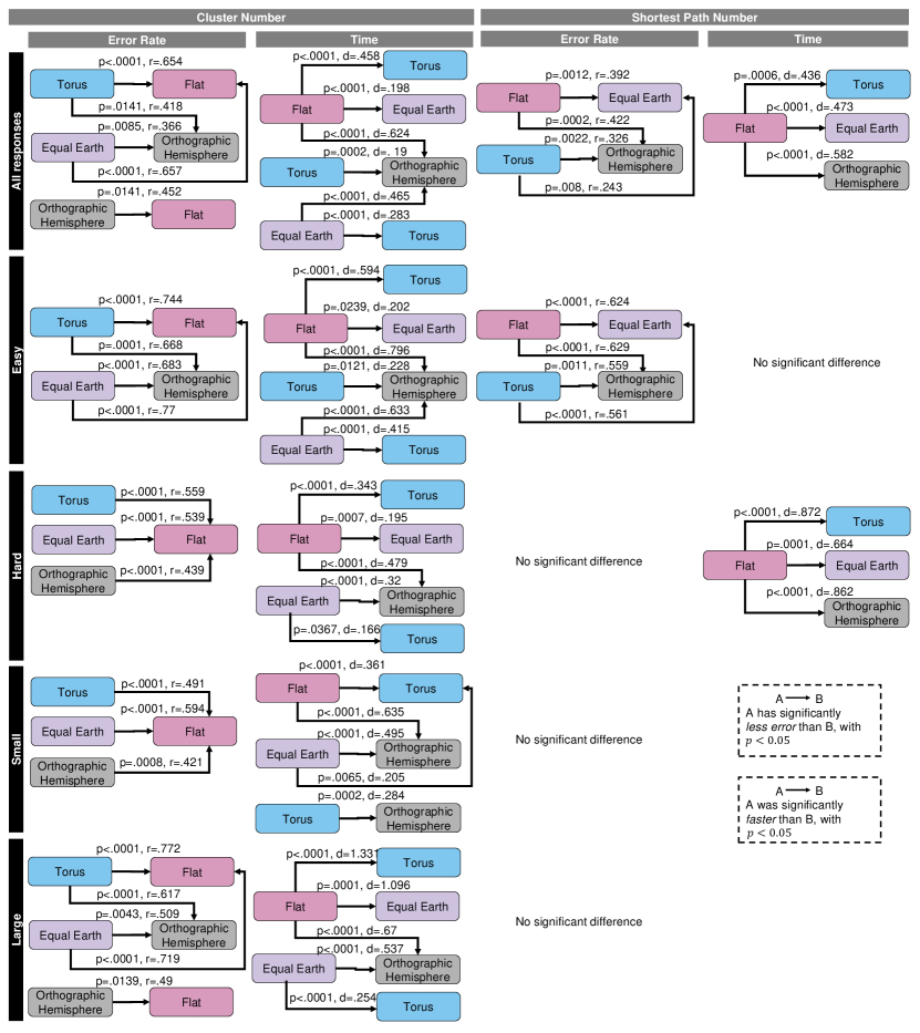
[Legend]
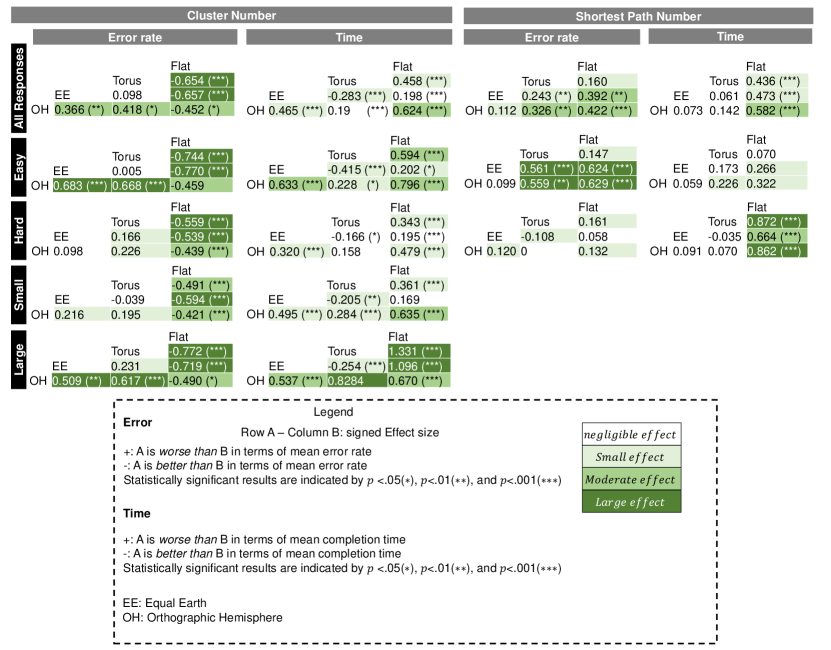
[Legend]

[Legend]