A passive admittance controller to enforce Remote Center of Motion and Tool Spatial constraints with application in hands-on surgical procedures

Abstract

The restriction of feasible motions of a manipulator link constrained to move through an entry port is a common problem in minimum invasive surgery procedures. Additional spatial restrictions are required to ensure the safety of sensitive regions from unintentional damage. In this work, we design a target admittance model that is proved to enforce robot tool manipulation by a human through a remote center of motion and to guarantee that the tool will never enter or touch forbidden regions. The control scheme is proved passive under the exertion of a human force ensuring manipulation stability, and smooth natural motion in hands-on surgical procedures enhancing the user’s feeling of control over the task. Its performance is demonstrated by experiments with a setup mimicking a hands-on surgical procedure comprising a KUKA LWR4+ and a virtual intraoperative environment.

1 Introduction

The vision of having robots work collaboratively with humans is slowly beginning to materialize in both industrial and professional robotics. In physical human-robot interaction (pHRI), humans can bring experience, knowledge, perception and understanding for the proper execution of a task and robots can reduce fatigue and increase human capabilities in terms of strength, speed and accuracy. There are tasks where the last manipulator link is constrained to move through an entry port, thus being only allowed to translate and rotate along its axis and rotate about the entry point. The existence of such a remote center of motion (RCM) constraint, if it is not incorporated in the robot’s controller, may lead to high cognitive load for the human as she/he has to account for them during the interaction. For example, in hands-on minimally invasive surgical procedures, the surgeon manipulates a long thin tool attached at the robot’s end-effector passing through an incision point on the patient’s body by exerting forces on the tool basis. Any such task is even more demanding when there are spatial constraints regarding the tool tip or the whole tool. In the surgical case, these spatial constraints concern sensitive tissues like arteries and veins that should not be accidentally injured during the operation. Hence the robot’s controller should further guarantee the avoidance of these regions and preferably provide a haptic feedback when the human manipulates the tool close to them.

In general, RCM and spatial constraints may either be real or desired. For example, in some surgical robots, the RCM constraint is achieved by mechanical means. If the robot is however a general purpose manipulator, the RCM should be imposed by the control action to ensure minimum stress of the incision wall. Spatial task constraints may either be hard constraints like the existence of a wall or rigid surface or soft constraints that should not be stressed by external forces according to the task. The latter is typical in surgical procedures in which forbidden region avoidance should be incorporated in the robot’s controller as it is essential for the patient’s safety. Even in tasks with hard spatial constraints, actively respecting them would decrease the physical and cognitive human effort.

In this work, we propose an admittance controller satisfying both RCM and forbidden region constraints during the robot’s kinesthetic guidance. As we shall see in the next subsection, the existing works in the literature, have addressed these two objectives separately either for autonomous or kinesthetic guidance cases. Control schemes have been proposed for industrial and minimum invasive surgical tasks for spatial constraint satisfaction. In surgery spatial constraints are related to forbidden regions. These constraints can be known analytically [1, 2, 3, 4, 5, 6], can be generated utilizing Dynamic Movement Primitives that encode the demonstration trajectory [7, 8] or provided as point clouds produced by the perception system [9, 10, 11, 12]. RCM enforcement schemes are mainly proposed for robotic assisted minimal invasive surgery (RAMIS) [13, 14, 15, 16, 17, 18, 19, 20, 21, 22, 23, 24, 25, 12, 26]. The proposed target admittance model is designed in a way that decouples the robot’s joint space into the RCM constrained and unconstrained subspace so that RCM constraints are satisfied during tool manipulation and the control action that guarantees manipulation away from the forbidden regions acts only along the RCM unconstrained directions. It is moreover proved passive under the exertion of a generalized human force which ensures manipulation stability in all cases. The proposed target admittance model, incorporates a novel variable damping term in order to achieve a smooth manipulation performance near the forbidden regions. Our experimental results in a virtual intraoperative environment, demonstrate that with our controller a user can effectively achieve intuitive RCM manipulation of a long tool away from forbidden areas providing haptic feedback in the form of repulsive forces when the tool is near them.

1.1 Related Works

Active constraints or virtual fixtures were firstly introduced in tele-robotic manipulation by Rosenberg providing force feedback from virtual environments to reduce the cognitive load of the user [27, 28] and have been utilized for both hands-on and teleportation applications in surgical [9, 6, 4, 5, 29, 12, 30] industrial [31, 32, 7, 2, 8] or even in underwater robotic tasks [11]. They can be classified as either virtual fixtures for enforcing barriers around forbidden regions [9, 1, 12, 10, 11, 30] or virtual fixtures for assisting guidance achieving an attractive behavior towards a desired path [6, 4, 5, 29, 7, 2, 8]. Notice that an attractive virtual fixture in a region can be assumed as a forbidden-region virtual fixture for its complementary space and vice versa. Their enforcement is implemented using energy storage methods, such as artificial potential fields [1, 3, 2, 8, 9, 7, 29, 12, 10, 11, 30] or via controllers that do not store energy [4, 5, 6]. The latter approach does not guarantee constraint satisfaction in all cases and is not able to provide haptic cues when the robot is not moving. Artificial potentials are unbounded [1, 9, 3, 2, 29] or bounded energy functions [8, 7, 10, 11, 12, 30] depending on the specific objective they address. For example, penetrated (bounded) artificial potentials are utilized around trajectories encoded by Dynamic Movement Primitives to allow a user to inspect kinesthetically as well as significantly modify a previously learned path [8, 7]. A method enforcing constraints utilizing unbounded functions are presented in [9] and [33] to guarantee that the robot tool tip and the whole tool respectively will never touch a forbidden surface provided by a point cloud. A review about artificial potential fields can be found in [34].

Tool manipulation via an RCM is typical in RAMIS where the tool is either directly manipulated by the surgeon or indirectly via a telemanipulation set-up. The former known as hands-on robotic surgery is preferred in some cases [30]. In hands-on robotic surgery the robot is under an impedance or admittance control scheme and the human force is directly applied on the tool. In teleoperated setups the surgeon manipulates a haptic device which generates velocities or displacements that are sent as reference velocities or positions respectively to the patient-side robot controller.

Different control approaches about the satisfaction of the RCM constraint and tool tip trajectory tracking have been proposed for autonomous operation or teleoperation set-ups  [18, 15, 22, 23, 24, 17, 16, 19, 20, 21]. Some of them require a torque level interface which is available in a limited number of the commercially available robotic manipulators [16, 15, 17]. In [15] the proposed solution constrains 3-dof instead of 2-dof that are required, by specifying a tool orientation compatible with the RCM given a desired tool-tip position trajectory. Unintentional external forces that may occur on the arm are mapped in the null space of the task. An optimization method is used in [23] to find the optimal joint configuration that satisfies the RCM constraint as well as reaching of a tool-tip target point but the controller may be trapped in a local minimum. In [24] a linear map is used, that transforms the velocity of the haptic device so that it satisfies the RCM constraint of the surgical robot. Works [18, 22] adopt a task priority approach with the RCM constraint being in the first priority level and the tool-tip trajectory tracking in the second. First order inverse kinematics are used and the approaches are validated only through simulations. In [20], [19] an inverse first order kinematic controller is designed to track a desired tip trajectory respecting the RCM constraint. All the above works do not provide proofs of stability and RCM constraint satisfaction.

There are limited works constraining the motion of the tool to satisfy a RCM in hands-on RAMIS procedures [26, 25, 12]. They also lack proof of closed loop system passivity and guarantees of RCM constraint satisfaction. In [13], we propose a control law applied at the torque level that required accurate knowledge of the robot’s dynamics and validate it through simulations. Its transfer to a real robot requires a robot with a torque interface and accurate knowledge of the dynamic parameters which is difficult in the majority of cases. To deal with this problem we have proposed an admittance control scheme in [14] ensuring passivity and manipulation of long instruments via a RCM. Methods proposed for teleoperated or autonomous operation cannot be directly applied in hands-on procedures particularly those proposing first order inverse kinematic solutions. If the human force is used in place of desired velocities or displacements in these methods, the zero target inertia which is implied negatively affects stability. In particular, as discussed in [35], the target inertia is lower bounded in order for the system to remain passive in a realistic admittance control case.

To the best of our knowledge spatial constraints together with RCM tool manipulation is only addressed in [21] and [12]. The authors in [21] propose a method to preserve the safety of sensitive human organs and achieve tip tracking by monitoring the minimum distance from the sensitive area or setting a threshold on the force exerted on the sensitive area in order to stop the robot. In [12] the authors propose a torque level control method for a RAMIS hands-on procedure. The RCM is achieved by regulating the tool to a desired orientation that is calculated to be compatible with the RCM constraint thus constraining 3-dof instead of 2-dof. Active constraints are imposed by producing repulsive forces on the tool shaft as the tool comes closer to the forbidden area defined by a point cloud. As the two controllers are superimposed, system dynamics are coupled with each controller affecting the performance of the other. Moreover, no proof or guarantees are provided that the tool will not touch the forbidden area or it will not enter the empty space between the points of the cloud.

1.2 Contributions

In this work, we address the problem of satisfying both RCM and forbidden region constraints via a novel admittance control design. A combination of our previous works [14] on RCM constraint and forbidden region constraint satisfaction [9], [33] produces a system that is not passive and consequently it cannot guarantee stability. In fact, we faced various stability problems when we had initially experimented with this control combination. We have thus redesigned the whole control scheme so that we can successfully address both objectives of RCM tool manipulation and spatial constraint enforcement close to forbidden areas via haptic feedback. The novel design is differentiated with respect to our previous works in several parts enumerated below.

1. The main novelty resides in the proposed mapping between the joint velocities and the free motion coordinates which differs from that of [14]. This novel mapping enables passivity to be proved in the presence of repulsive potential and it allows free motion coordinates to be defined in correspondence to the force components in a decoupled, independent way. The resulted motion is thus intuitive, enhancing transparency of manipulation. In contrast, the respective mapping in [14], generates free coordinatecouplings leading to counter intuitive motion.

2. In this work, the null space basis of the RCM constraint Jacobian is designed analytically as opposed to the algorithmic on-line solution utilized in [14] which adds computational load to the overall solution and may result in discontinuities that affect manipulation performance.

3. A novel variable damping term is incorporated in the target admittance dynamics proposed in this work, which is instrumental in achieving a smooth performance in the presence of the repulsive potentials that are introduced to enforce forbidden areas. As the introduction of such repulsive potentials is equivalent to a non-linear increase of the apparent stiffness in the vicinity of the constraints, the constant damping utilized in [14] jeopardizes performance.

4. The method to enforce forbidden area constraints for the tool presented in our previous works [9], [33] does not consider RCM constraints and is implemented in the torque level via an impedance controller. In this work, we propose an admittance model which is shaped by the presence of the RCM constraints, so that repulsive forces are filtered. It is consequently not obvious that the sensitive areas will be protected. An essential contribution of this work is that we prove that active constraint satisfaction is guaranteed by the proposed scheme in all practical cases.

Summarising, the contribution of this work is a novel admittance control scheme that:

• guarantees stability of the overall system via passivity, achieving both objectives of RCM and sensitive area constraint satisfaction as testified by the theoretical proofs and validated by the experimental results

• provides manipulation transparency and smooth motion in hands-on surgical procedures which enhances the user’s feeling of control over the task.

The rest of the paper is organized as follows. Section 2 introduces the problem and the control design objectives. Section 3 summarises our background work on RCM constraint formulation and repulsive artificial potential fields for forbidden areas given as point clouds. Section 4 presents the proposed admittance control scheme and proofs of passivity and control objectives achievement. The analysis for the active constraint enforcement is extended to the whole tool body in subsection 4.3 and the designed variable damping is presented in subsection 4.4. Experimental results that demonstrate its effectiveness in a set-up mimicking a hands-on surgical procedure are presented in Section 5. Conclusions are drawn in Section 6.

2 Problem Description

Consider a general purpose robot with $n\geq 6$ degrees of freedom, which can be kinematically controlled that is common in most of the commercially available robotic equipment. The latter means that the robot is provided by an interface that accepts position or velocity reference commands and its internal controller ensures negligible errors in tracking them. Let a force/torque sensor be attached at its end-effector holding a long thin tool that is directly manipulated by a human through an entry port. Further consider the availability of a point cloud of an object characterized as a forbidden area that should not be touched by the tool. The task is the kinesthetic guidance of the tool to any accessible area through the port never touching the forbidden area. These type of tasks are typically encountered in hands-on robotic surgery.

The aim of this work is to design an admittance controller that would simultaneously achieve the following:

• the entry port will be imposed as a RCM to the tool’s manipulation by the guiding human

• the tool-tip or the tool body will never enter or even touch the forbidden area

• the user will feel repulsive forces in the vicinity of the forbidden area

• the controlled system will be passive with respect to the forces exerted by the user

• a smooth tool manipulation performance is ensured close to forbidden areas

The entry port may be either rigidly or softly attached to the surrounding environment as in the surgical applications. Then respectively, the first objective means that constraint forces or entry port displacement will be effectively zero during the task. The point cloud of the forbidden area is assumed to be provided by a camera registered in the robot’s workspace like an endoscopic camera capturing intraoperative images in surgery. Smooth tool manipulation refers to lack of tool oscillatory behaviour.

3 Background

For completeness and clarity, the RCM constraint formulation and repulsive artificial potential are presented in this section, with more details to be found in our previous works [14] and [9] respectively.

3.1 RCM constraint formulation

Let the position and the orientation of the tool-tip be given by $\mathbf{p}_{t}\in\mathbb{R}^{3},\ \mathbf{R}_{t}=[\mathbf{a}_{t}\ \mathbf{o}_{t}\ \mathbf{n}_{t}]\in\mathbb{R}^{3\times 3}$ respectively. Without loss of generality the unit direction of the tool is assumed to be $\mathbf{n}_{t}$. Let the entry port position $\mathbf{p}_{c}\in\mathbb{R}^{3}$ be known. A way to find it, is for example, to manually guide the tool tip to the entry port to record its position in the robot’s space. Given an initial robot configuration such that the tool axis $\mathbf{n}_{t}$ passes through $\mathbf{p}_{c}$ we aim to impose $\mathbf{p}_{c}\$as a RCM constraint during the manipulation of the tool by the user. Hence, the projection of $\mathbf{p}_{t}-\mathbf{p}_{c}$ on the plane orthogonal to $\mathbf{n}_{t}$ is desired to be kept close to zero at all times (see Figure 1).

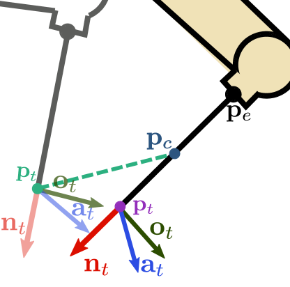
Figure 1: Two poses of the robot tool with tip frames and the RCM point $\mathbf{p}_{c}$, passing through RCM (bold) and with an offset (grey).

Notice that $\mathbf{B}_{c}=[\mathbf{a}_{t}\ \mathbf{o}_{t}]\in\mathbb{R}^{3\times 2}$ is a basis of this plane since $\mathbf{n}_{t}^{\mathrm{T}}\mathbf{B}_{c}=\mathbf{0}_{1\times 2}$. Then, the desired RCM constraint is expressed as follows:

$$\mathbf{x}_{c}\triangleq\mathbf{B}^{\mathrm{T}}_{c}(\mathbf{p}_{t}-\mathbf{p}_{c})=\mathbf{0}.$$ (1)

Taking the time derivative of (1), yields the following velocity constraint:

$$\dot{\mathbf{x}}_{c}=\mathbf{B}^{\mathrm{T}}_{c}\dot{\mathbf{p}}_{t}+\dot{\mathbf{B}}^{\mathrm{T}}_{c}(\mathbf{p}_{t}-\mathbf{p}_{c})=\mathbf{0}.$$ (2)

By definition $\mathbf{R}_{t}=[\mathbf{B}_{c}\ \mathbf{n}_{t}]$ and using the property $\mathbf{\dot{R}}_{t}=\bm{\widehat{\omega}}_{t}\mathbf{R}_{t}$, with $\widehat{(.)}$ denoting the skew symmetric matrix of a 3-d vector, we get: $\dot{\mathbf{B}}_{c}=\bm{\widehat{\omega}}_{t}{\mathbf{B}}_{c}.$ Thus (2) becomes:

$$\dot{\mathbf{x}}_{c}:=\mathbf{A}_{x}\mathbf{v}_{t}=\mathbf{0}$$ (3)

where $\mathbf{A}_{x}$ is the constraint Jacobian in the task space:

$$\mathbf{A}_{x}=\mathbf{B}^{\mathrm{T}}_{c}[\mathbf{I}_{3\times 3}\ \ {(\mathbf{p}_{t}-\mathbf{p}_{c})^{\wedge}}]\in\mathbb{R}^{2\times 6}.$$ (4)

Notice that by definition this is a full rank matrix (rank 2). Let $\mathbf{J_{t}}(\mathbf{q}_{d})\in\mathbb{R}^{6\times n}$ be the robot Jacobian which maps the joint velocities $\mathbf{\dot{q}}_{d}$ to the generalized velocity of the tool-tip $\mathbf{v}_{t}=[\dot{\mathbf{p}}_{t}^{\mathrm{T}}\ \bm{\omega}_{t}^{\mathrm{T}}]^{\mathrm{T}}\in\mathbb{R}^{6}$ i.e.:

$$\mathbf{v}_{t}=\mathbf{J}_{t}(\mathbf{q}_{d})\mathbf{\dot{q}}_{d}$$ (5)

where $\dot{\mathbf{p}}_{t},\ \bm{\omega}_{t}\in\mathbb{R}^{3}$ are the linear and angular velocities of the tool-tip. We can therefore utilize (5) to express (3) in the robot’s joint space:

$$\dot{\mathbf{x}}_{c}:=\mathbf{A}\dot{\mathbf{q}}_{d}=\mathbf{0}$$ (6)

where

$$\mathbf{A}=\mathbf{A}_{x}\mathbf{J}_{t}(\mathbf{q}_{d})\in\mathbb{R}^{2\times n}$$ (7)

denotes the constraint Jacobian in the joint space. Notice that matrix $\mathbf{A}$ is full rank assuming a motion away from kinematic singularities.

3.2 Artificial potentials for active constraint enforcement

Let the surface of the forbidden region be approximated by a finite set of points $\mathcal{O}_{s}$ with positions $\mathbf{p}_{i}$. Let $\rho\in\mathbb{R}^{+}$ be the density of $\mathcal{O}_{s}$ in points per $cm^{3}$ which is considered known and homogeneous. Then the side of a cube which includes one point is $\dfrac{1}{\sqrt[3]{\rho}}$. To cover the empty space between the points in $\mathcal{O}_{s}$ we create spheres with radius $d_{c}=\frac{\sqrt{3}}{2\sqrt[3]{\rho}}$ centered at each point $\mathbf{p}_{i}$ so that each one contains one cube. We can thus guarantee empty space coverage by overlapping spheres. We then define the constrained surface as the boundary $\partial\mathcal{O}_{c}$ of the overlapping spheres $\mathcal{O}_{c}$ (see Figure 2):

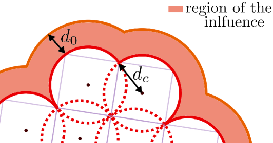
Figure 2: Visualization of a cross section of the forbidden region with the overlapping spheres and the region of influence of the repulsive potential field.

$$\mathcal{O}_{c}=\bigcup_{\mathbf{p}_{i}\in\mathcal{O}_{s}}\{\mathbf{x}\in\mathbb{R}^{3}:\|\mathbf{x}-\mathbf{p}_{i}\|\leq d_{c}\}.$$ (8)

To ensure that the the boundary $\partial\mathcal{O}_{c}$ will never be penetrated or even touched we aim to impose a repulsive artificial potential with a predefined range of influence $d_{0}$ so that the user is repelled away from the forbidden area when the tip is approaching it by a distance less than $d_{0}$.

In particular, for each point of the cloud we utilize a field function $V_{i}(\mathbf{p}_{t})$ with the following properties:

• $V_{i}(\mathbf{p}_{t})=V(\|\mathbf{p}_{t}-\mathbf{p}_{i}\|)$ is a positive continuously differentiable scalar function, for all $\|\mathbf{p}_{t}-\mathbf{p}_{i}\|\in(d_{c},d_{c}+d_{0}];$

• $V_{i}(\mathbf{p_{t}})\rightarrow\infty$ if only if $\|\mathbf{p}_{t}-\mathbf{p}_{i}\|\rightarrow d_{c};$

• $\frac{\partial V_{i}(\mathbf{p}_{t})}{\partial\mathbf{p}_{t}}$ is zero if and only if $\|\mathbf{p}_{t}-\mathbf{p}_{i}\|\geq d_{c}+d_{0}$.

In particular, the following function introduced in our previous work [9] is utilized:

$$V_{i}(\mathbf{p}_{t})=\begin{cases}{\dfrac{k_{i}}{2}\ln\left(\frac{1}{1-\psi_{i}}\right)^{2},}&\quad\text{if}\ \|\mathbf{p}_{t}-\mathbf{p}_{i}\|\leq d_{c}+d_{0},\\ \text{0,}&\quad\text{else}\\ \end{cases}$$ (9)

where $k_{i}>0$ is a scalar gain and

$$\psi_{i}=\frac{(\|\mathbf{p_{t}}-\mathbf{p}_{i}\|-(d_{0}+d_{c}))^{2}}{d_{0}^{2}}$$ (10)

This field function is depicted in Figure 3 for increasing values of $k_{i}$.

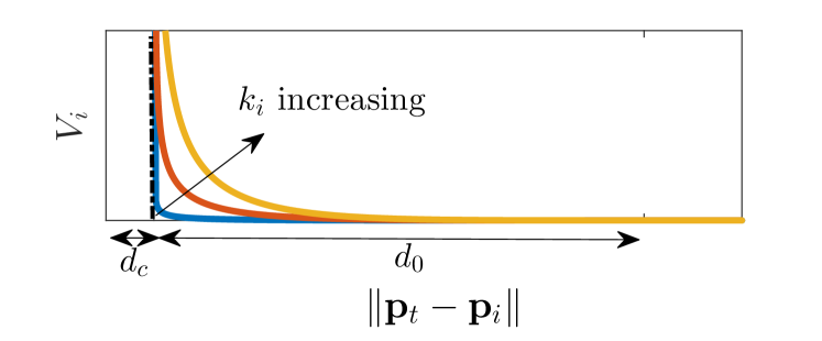
Figure 3: The repulsive artificial potential field (9) with respect to the distance of the tool-tip from a point of the cloud of the forbidden region.

Notice that this repulsive potential field is zero beyond the range of influence and tends to infinity at the sphere boundary. Hence $V_{i}<\infty$ if and only if $\psi_{i}<1$ which is satisfied if and only if $\|\mathbf{p_{t}}-\mathbf{p}_{i}\|>d_{c}$.

The negative gradient $-\dfrac{\partial V_{i}}{\partial\mathbf{p_{t}}}$ of each $V_{i}$ (9) produce repulsive forces at the tool tip $\mathbf{f}_{i}(\mathbf{p}_{t})\in\mathbb{R}^{3}$:

$$\mathbf{f}_{i}(\mathbf{p}_{t})=\begin{cases}{k_{vi}\mathbf{e}_{i}}&\quad\text{if}\ \|\mathbf{p}_{t}-\mathbf{p}_{i}\|\leq d_{c}+d_{0},\\ \text{0,}&\quad\text{else}\\ \end{cases}$$ (11)

where

$$\mathbf{e}_{i}=\left((d_{0}+d_{c})-\|\mathbf{p}_{t}-\mathbf{p}_{i}\|\right)\frac{\mathbf{p}_{t}-\mathbf{p}_{i}}{\|\mathbf{p}_{t}-\mathbf{p}_{i}\|}\in\mathbb{R}^{3}$$ (12)

is a vector with magnitude equal to the distance between the tool-tip and the sphere of radius $d_{0}+d_{c}$ centered at $\mathbf{p}_{i}$ with direction pointing from the center of the sphere towards the tool-tip, and

$$k_{vi}=\dfrac{2k_{i}}{d_{0}^{2}(1-\psi_{i})}\ln\left(\frac{1}{1-\psi_{i}}\right)\in\mathbb{R}.$$ (13)

This scalar gain can be interpreted as a variable stiffness within the range of the field’s influence which increases as the distance of tool-tip to the sphere surface decreases. Let the sum of repulsive forces produced by each artificial potential field $\mathbf{f}_{i}$ be:

$$\mathbf{f}_{r}=\sum_{\mathbf{p}_{i}\in\mathcal{O}_{s}}\mathbf{f}_{i}.$$ (14)

In [9], (14) is utilized to achieve enforcement of the constrained surface $\partial\mathcal{O}_{c}$ via an impedance control scheme without RCM considerations.

4 The Proposed Admittance Control Scheme

Our aim is to design an admittance model that decouples the robot’s joint space into the two spaces of the RCM constrained and unconstrained motion. To this aim, we initially find a basis for the null space of the RCM constraint Jacobian, and then we proceed in the design of the desired target admittance model that is proved to fulfill all of the objectives set in section 2. Details on the extension of the forbidden area repulsive forces for the whole tool and the variable damping gains are given in separate subsections.

4.1 Null RCM constraint space

We propose a basis for the null space of $\mathbf{A}_{x}$ in which any forces should lie in order to avoid affecting the RCM constraint space. Let, this basis be denoted by matrix $\mathbf{Z}_{x}\in\mathbb{R}^{4\times 6}$ which should be composed of vectors that are linearly independent and span the null space of matrix $\mathbf{A}_{x}$ i.e. $\mathbf{A}_{x}\mathbf{Z}_{x}^{\mathrm{T}}=\mathbf{0}_{2\times 4}$. The following basis $\mathbf{Z}_{x}$ for the null space of $\mathbf{A}_{x}$ is proposed:

$$\mathbf{Z}_{x}=\begin{bmatrix}\ \ \ \ {\mathbf{n}}_{t}^{\mathrm{T}}\ \ \ \ \ \mathbf{0}_{1\times 3}\\ (\mathbf{p}_{t}-\mathbf{p}_{c})^{\wedge}\ \ \mathbf{I}_{3\times 3}\end{bmatrix}$$ (15)

Equivalently for the joint space we need to find a basis of the null space of the constraint Jacobian $\mathbf{A}$. Let this basis be denoted by $\mathbf{Z}\in\mathbb{R}^{(n-2)\times n}$ which should satisfy the following equation:

$$\mathbf{A}\mathbf{Z}^{\mathrm{T}}=\mathbf{0}\in\mathbb{R}^{2\times(n-2)}.$$ (16)

The following is a valid solution incorporating $\mathbf{Z}_{x}$:

$$\mathbf{Z}=\begin{bmatrix}\mathbf{Z}_{x}(\mathbf{J}_{t}\mathbf{J}_{t}^{\mathrm{T}})^{-1}\mathbf{J}_{t}\\ \mathbf{G}\end{bmatrix}\in\mathbb{R}^{(n-2)\times n}$$ (17)

where $\mathbf{G}\in\mathbb{R}^{(n-6)\times n}$ is the base matrix of the null space of $\mathbf{J}_{t}$ in case $n>6$ i.e. $\mathbf{G}\mathbf{J}_{t}^{\mathrm{T}}=\mathbf{0}$ defined as in [36]. We can easily verify (16) for $\mathbf{Z}$ given by (17).

Remark 1.

Notice that the null space basis for the task in the joint space, $\mathbf{Z}_{x}(\mathbf{J}_{t}\mathbf{J}_{t}^{\mathrm{T}})^{-1}\mathbf{J}_{t}$, is here designed analytically as opposed to the algorithmic on-line solution utilized in our previous work [14] which adds computational load to the overall solution but more importantly, it may result in discontinuities that affect manipulation performance.

A general solution for the inverse of the constraint motion kinematics $\dot{\mathbf{x}}_{c}=\mathbf{A}\dot{\mathbf{q}}_{d}$ is given by:

$$\dot{\mathbf{q}}_{d}=\mathbf{A}^{\dagger}\dot{\mathbf{x}}_{c}+(\mathbf{I}_{n\times n}-\mathbf{A}^{\dagger}\mathbf{A})\bm{\mathbf{\xi}}$$ (18)

where $\mathbf{A}^{\dagger}=\mathbf{W}^{-1}\mathbf{A}^{\mathrm{T}}(\mathbf{A}\mathbf{W}^{-1}\mathbf{A}^{\mathrm{T}})^{-1}\in\mathbb{R}^{n\times 2}$ is the weighted right pseudoinverse of $\mathbf{A}$ for a symmetric positive definite matrix of weights $\mathbf{W}$ and $\bm{\mathbf{\xi}}\in\mathbb{R}^{n}$ denotes an arbitrary vector. Denote the velocity of the unconstrained kinematics by $\dot{\mathbf{x}}_{f}\in\mathbb{R}^{(n-2)}$. This velocity should be mapped in the joint space by $\mathbf{Z}^{\mathrm{T}}$ in order not to affect the constraint motion since $(\mathbf{I}_{n\times n}-\mathbf{A}^{\dagger}\mathbf{A})\mathbf{Z}^{\mathrm{T}}=\mathbf{Z}^{\mathrm{T}}$. Thus, (18) can be written in a compact form as:

$$\dot{\mathbf{q}}_{d}=\mathbf{S}\begin{bmatrix}\dot{\mathbf{x}}_{c}\\ \dot{\mathbf{x}}_{f}\end{bmatrix}$$ (19)

where $\mathbf{S}=[\mathbf{A}^{\dagger}\ \mathbf{Z}^{\mathrm{T}}]\in\mathbb{R}^{n\times n}.$ Let the weighted right pseudoinverse of $\mathbf{Z}$ be defined by $\mathbf{Z}^{\dagger}=\mathbf{W}\mathbf{Z}^{\mathrm{T}}(\mathbf{Z}\mathbf{W}\mathbf{Z}^{\mathrm{T}})^{-1}\in\mathbb{R}^{n\times(n-2)}$. Then the following properties hold between $\mathbf{A}$, $\mathbf{Z}$ and their pseudoinverses:

1. $\mathbf{A}\mathbf{A}^{\dagger}=\mathbf{I}_{2\times 2}$

2. $\mathbf{Z}^{{\dagger}^{\mathrm{T}}}\mathbf{A}^{\dagger}=\mathbf{0}_{(n-2)\times 2}$

3. $\mathbf{Z}\mathbf{Z}^{{\dagger}}=\mathbf{Z}^{{\dagger}^{\mathrm{T}}}\mathbf{Z}^{\mathrm{T}}=\mathbf{I}_{(n-2)\times(n-2)}$

To recover the constraint velocity $\dot{\mathbf{x}}_{c}$ and the free space velocity $\dot{\mathbf{x}}_{f}$ from (19), the inverse of $\mathbf{S}$ such that $\mathbf{S}^{-1}\mathbf{S}=\mathbf{I}_{n\times n}$ is easily found utilizing the above properties and (16) to be:

$$\mathbf{S}^{-1}=\begin{bmatrix}\mathbf{A}\\ \mathbf{Z}^{{\dagger}^{\mathrm{T}}}\end{bmatrix}\in\mathbb{R}^{n\times n}.$$ (20)

Thus, the following forward kinematic mapping holds:

$$\begin{bmatrix}\dot{\mathbf{x}}_{c}\\ \dot{\mathbf{x}}_{f}\end{bmatrix}=\begin{bmatrix}\mathbf{A}\\ \mathbf{Z}^{{\dagger}^{\mathrm{T}}}\end{bmatrix}\dot{\mathbf{q}}_{d}.$$ (21)

which decouples RCM constrained and unconstrained motion since it satisfies the following properties for all nonzero $\mathbf{\dot{x}}_{f}$ and $\mathbf{\dot{x}}_{c}$ [37]:

$$\mathbf{A}\mathbf{S}\begin{bmatrix}\mathbf{0}\\ \dot{\mathbf{x}}_{f}\end{bmatrix}=\mathbf{0},\ \mathbf{Z}^{{\dagger}^{\mathrm{T}}}\mathbf{S}\begin{bmatrix}\dot{\mathbf{x}}_{c}\\ \mathbf{0}\end{bmatrix}=\mathbf{0}.$$

Hence, the velocity in the free space does not affect the velocity in the RCM constraint space and vice versa.

Remark 2.

Notice that the proposed mapping between the joint velocities $\dot{\mathbf{q}}_{d}$ and the free motion coordinates $\dot{\mathbf{x}}_{f}$ in eq (21) differs from that of [14], which utilizes the $\mathbf{Z}\mathbf{W}$ matrix instead of the $\mathbf{Z}^{{\dagger}^{T}}$ transpose of this work. The proposed mapping enables passivity to be proved in the presence of repulsive potentials which is lost if the mapping of [14] is utilized.

4.2 Target admittance model

We are now ready to propose the following target dynamics to achieve all our control objectives:

$$\begin{split}\ddot{{\mathbf{q}}}_{d}+\mathbf{S}\begin{bmatrix}\mathbf{h}\\ \mathbf{u}\end{bmatrix}=\mathbf{Z}^{\mathrm{T}}\mathbf{Z}\mathbf{J}_{t}^{\mathrm{T}}\bigg{(}\mathbf{F}_{th}+\mathbf{F}_{r}\bigg{)}\end{split}$$ (22)

where

$$\begin{split}\mathbf{h}=\dot{\mathbf{A}}\dot{\mathbf{q}}_{d}+2\alpha\dot{\mathbf{x}}_{c}+\beta^{2}\mathbf{x}_{c},\ \ \mathbf{u}=\bigg{(}\mathbf{D}_{f}\mathbf{Z}^{{\dagger}^{\mathrm{T}}}+\dfrac{d(\mathbf{Z}^{{\dagger}^{\mathrm{T}}})}{dt}\bigg{)}\dot{\mathbf{q}}_{d}\end{split}$$ (23)

with $\mathbf{D}_{f}\in\mathbb{R}^{(n-2)\times(n-2)}$ being a diagonal matrix of positive damping gains, $\alpha,\ \beta$ are positive gains, $\mathbf{F}_{r}=\begin{bmatrix}{\mathbf{f}}_{r}\\ \mathbf{0}_{3\times 1}\end{bmatrix}\in\mathbb{R}^{6\times 1}$ is the total repulsive force at the tip, and $\mathbf{F}_{th}\in\mathbb{R}^{6}$ is the human generalized force transformed in the tool-tip. In particular, if the user exerts the generalized force $\mathbf{F}_{h}\in\mathbb{R}^{6}$, at the end-effector (tool basis) then $\mathbf{F}_{th}=\mathbf{T}_{te}\mathbf{F}_{h}$ with $\mathbf{T}_{te}=\begin{bmatrix}\ \ \ \mathbf{I}_{3\times 3}\ \ \ \ \ \ \mathbf{0}_{3\times 3}\\ (\mathbf{p}_{e}-\mathbf{p}_{t})^{\wedge}\ \ \mathbf{I}_{3\times 3}\end{bmatrix}$ where $\mathbf{p}_{e}$ is the position of the end-effector w.r.t. the base frame. The selection of gains is detailed in the rest of this section. Target dynamics (22), (23) are integrated to produce joint motion references $\mathbf{q}_{d},\dot{\mathbf{q}}_{d}$ to the robot which is assumed to faithfully reproduce them. The next theorem and its proof describes the main result of the proposed admittance controller.

Theorem 1.

The following statements for the target dynamics (22), (23) with initial joint position $\mathbf{q}_{d}(t_{0})$ such that $\mathbf{p}_{t}(t_{0})\notin\mathcal{O}_{c}$ are valid:

1. the dynamics of the RCM-constraint space are decoupled from the dynamics in the free space.

2. $\dot{\mathbf{x}}_{c}$, ${\mathbf{x}}_{c}$ converge exponentially to zero.

3. the system is strictly output passive with respect to the velocity $\dot{\mathbf{x}}_{f}$, under the exertion of a generalized human force

4. the forbidden region is never violated

Proof.

Taking the time derivative of $\dot{\mathbf{x}}_{c}$ from (21) and substituting $\ddot{\mathbf{q}}_{d}$ from (22), yields the constraint motion dynamics:

$$\begin{split}\ddot{\mathbf{x}}_{c}=-\mathbf{A}\mathbf{S}\begin{bmatrix}\mathbf{h}\\ \mathbf{u}\end{bmatrix}+\mathbf{A}\mathbf{Z}^{\mathrm{T}}\mathbf{Z}\mathbf{J}_{t}^{\mathrm{T}}\bigg{(}\mathbf{F}_{th}+{\mathbf{F}_{r}}\bigg{)}+\dot{\mathbf{A}}\dot{\mathbf{q}}_{d}.\end{split}$$ (24)

Utilizing property (i) and (16) it is easy to show that $\mathbf{A}\mathbf{S}=[\mathbf{I}_{2\times 2}\ \ \mathbf{0}_{2\times(n-2)}]$. Substituting $\mathbf{h}$ from (23) in (24) yields the exponentially stable constraint motion dynamics:

$$\ddot{\mathbf{x}}_{c}+2\alpha\dot{\mathbf{x}}_{c}+\beta^{2}{\mathbf{x}}_{c}=0.$$ (25)

which ensure that ${\mathbf{x}}_{c}$ and $\dot{\mathbf{x}}_{c}$ will converge exponentially to zero completing the proof of theorem’s statement (2). It is now clear that the $\mathbf{h}$ term in (22) is instrumental in yielding the above linear exponentially stable system for the constraint space motion. Parameters $\alpha$ and $\beta$ are equal for a critically damped response and their value determines the speed of exponential convergence of $\mathbf{x}_{c}$ to zero. Notice that the set:

$${{\mathcal{S}}\triangleq\left\{(\mathbf{q}_{d},\dot{\mathbf{q}}_{d})\in\mathbb{R}^{2n}\mid\dot{\mathbf{x}}_{c}=0,\mathbf{x}_{c}=0\right\}}$$ (26)

is positively invariant. In other words, once a trajectory of the system starts or enters ${\mathcal{S}}$ it will evolve within this set for all times. Within this set, (19) becomes $\dot{\mathbf{q}}_{d}=\mathbf{Z}^{\mathrm{T}}\dot{\mathbf{x}}_{f}$; left multiplied by $\mathbf{J}_{t}$ yields the generalized tip velocity ${\mathbf{v}}_{t}=\mathbf{Z}_{x}^{\mathrm{T}}\dot{\mathbf{x}}_{f_{\{1:4\}}}$ which clarifies the physical meaning of the free motion velocity coordinates $\dot{\mathbf{x}}_{f}$; the first is a linear velocity in the direction of the tool axis, the next three correspond to the angular velocity while the remaining $n-6$ coordinates refer to the robot’s redundant dof.

Taking the time derivative of $\dot{\mathbf{x}}_{f}$ from (21) and substituting $\ddot{\mathbf{q}}_{d}$ from (22), yields:

$$\begin{split}\ddot{{\mathbf{x}}}_{f}=-\mathbf{Z}^{{\dagger}^{\mathrm{T}}}\mathbf{S}\begin{bmatrix}\mathbf{h}\\ \mathbf{u}\end{bmatrix}+\mathbf{Z}^{{\dagger}^{\mathrm{T}}}\mathbf{Z}^{\mathrm{T}}\mathbf{Z}\mathbf{J}_{t}^{\mathrm{T}}\bigg{(}\mathbf{F}_{th}+{\mathbf{F}_{r}}\bigg{)}+\dfrac{d(\mathbf{Z}^{{\dagger}^{\mathrm{T}}})}{dt}\dot{\mathbf{q}}_{d}.\end{split}$$

Utilizing properties (ii) and (iii) it is easy to show that $\mathbf{Z}^{{\dagger}^{\mathrm{T}}}\mathbf{S}=[\mathbf{0}_{(n-2)\times 2}\ \ \mathbf{I}_{(n-2)\times(n-2)}]$. Thus, substituting $\mathbf{u}$ from (23) yields the free space motion dynamics:

$$\begin{split}\ddot{\mathbf{x}}_{f}+\mathbf{D}_{f}\dot{\mathbf{x}}_{f}=\mathbf{Z}\mathbf{J}_{t}^{\mathrm{T}}\bigg{(}\mathbf{F}_{th}+{\mathbf{F}_{r}}\bigg{)}\end{split}$$ (27)

Remark 3.

Notice that $\mathbf{Z}\mathbf{J}_{t}^{\mathrm{T}}=\begin{bmatrix}\mathbf{Z}_{x}\\ \mathbf{0}_{(n-6)\times 6}\end{bmatrix}$. Hence any forces multiplied by $\mathbf{Z}_{x}$ (15) results in forces along the tool axis and torques around the entry port. Thus in (27) there is a correspondence between the free motion velocity coordinates and the filtered force components $\mathbf{Z}_{x}(\mathbf{F}_{th}+{\mathbf{F}_{r}})$ that leads to an intuitive motion under the exerted force. In fact, the first component of $\dot{\mathbf{x}}_{f}$ is a linear velocity in the direction of the tool axis and the next three components correspond to the angular velocity. This natural correspondence is lacking from [14].

It is clear that $\mathbf{D}_{f}$ introduces damping along the coordinates of $\mathbf{\dot{x}}_{f}$. Damping gains for the angular velocity coordinates $\dot{\mathbf{x}}_{f_{\{2:4\}}}$ should be equal for a synchronized response. Thus proof of statement (1) regarding the decoupling of free motion dynamics (27) from the constraint dynamics (25) is completed.

For the proof of statement (3) consider the following candidate Lyapunov function:

$$V_{f}=\dfrac{1}{2}\dot{\mathbf{x}}_{f}^{\mathrm{T}}\dot{\mathbf{x}}_{f}+\sum_{\mathbf{p}_{i}\in\mathcal{O}_{s}}{V}_{i}(\mathbf{p}_{t}).$$ (28)

Its time derivative along the set $\mathcal{S}$ by substituting $\ddot{\mathbf{x}}_{f}$ from (27), is given by:

$$\begin{split}\dot{V}_{f}=&-\dot{\mathbf{x}}_{f}^{\mathrm{T}}\mathbf{D}_{f}\dot{\mathbf{x}}_{f}+\dot{\mathbf{x}}_{f}^{\mathrm{T}}\mathbf{Z}\mathbf{J}_{t}^{\mathrm{T}}\bigg{(}\mathbf{F}_{th}+{\mathbf{F}_{r}}\bigg{)}-{\mathbf{F}_{r}}^{\mathrm{T}}{\mathbf{v}}_{t}.\end{split}$$ (29)

Substituting ${\mathbf{v}}_{t}$ from (5) yields:

$$\begin{split}\dot{V}_{f}&=-\dot{\mathbf{x}}_{f}^{\mathrm{T}}\mathbf{D}_{f}\dot{\mathbf{x}}_{f}+\dot{\mathbf{x}}_{f}^{\mathrm{T}}\mathbf{Z}\mathbf{J}_{t}^{\mathrm{T}}\bigg{(}\mathbf{F}_{th}+{\mathbf{F}_{r}}\bigg{)}-{\mathbf{F}_{r}}^{\mathrm{T}}\mathbf{J}_{t}\dot{\mathbf{q}}_{d}.\end{split}$$ (30)

Furthermore, substituting $\dot{\mathbf{q}}_{d}$ from (19) in the invariant set $\mathcal{S}$ yields:

$$\begin{split}\dot{V}_{f}=-\dot{\mathbf{x}}_{f}^{\mathrm{T}}\mathbf{D}_{f}\dot{\mathbf{x}}_{f}+\dot{\mathbf{x}}_{f}^{\mathrm{T}}\mathbf{Z}\mathbf{J}_{t}^{\mathrm{T}}\ \mathbf{F}_{th}\end{split}$$ (31)

which implies that the output $\dot{\mathbf{x}}_{f}$ is strictly passive under the exertion of the filtered human generalized force $\mathbf{Z}\mathbf{J}_{t}^{\mathrm{T}}\ \mathbf{F}_{th}$.

Rewriting (31) by completing the squares, yields:

$$\begin{split}\dot{V}_{f}=&-||\sqrt{\mathbf{D}_{f}}\dot{\mathbf{x}}_{f}-\dfrac{1}{2}\sqrt{\mathbf{D}_{f}}^{-1}\mathbf{Z}\mathbf{J}_{t}^{\mathrm{T}}\ \mathbf{F}_{th}||^{2}\\ &+\dfrac{1}{4}\mathbf{F}_{th}^{\mathrm{T}}\mathbf{J}_{t}\mathbf{Z}^{\mathrm{T}}\mathbf{D}_{f}^{-1}\mathbf{Z}\mathbf{J}_{t}^{\mathrm{T}}\ \mathbf{F}_{th}\leq\dfrac{1}{4}\mathbf{F}_{th}^{\mathrm{T}}\mathbf{J}_{t}\mathbf{Z}^{\mathrm{T}}\mathbf{D}_{f}^{-1}\mathbf{Z}\mathbf{J}_{t}^{\mathrm{T}}\ \mathbf{F}_{th}\end{split}$$ (32)

Notice that $\mathbf{F}_{h}$ represents the force applied by the human to guide the robot. Thus, $\mathbf{F}_{h}$ is bounded and therefore $\mathbf{F}_{th}$ and $\mathbf{F}_{th}^{\mathrm{T}}\mathbf{J}_{t}\mathbf{Z}^{\mathrm{T}}\mathbf{D}_{f}^{-1}\mathbf{Z}\mathbf{J}_{t}^{\mathrm{T}}\ \mathbf{F}_{th}$ are also bounded functions of time. Additionally, the human forces have bounded energy. Hence integrating (32) we get:

$$V_{f}\leq V_{f}(t_{0})+\int\dfrac{1}{4}\mathbf{F}_{th}^{\mathrm{T}}\mathbf{J}_{t}\mathbf{Z}^{\mathrm{T}}\mathbf{D}_{f}^{-1}\mathbf{Z}\mathbf{J}_{t}^{\mathrm{T}}\ \mathbf{F}_{th}<\infty.$$ (33)

Thus, ${V}_{i}(\mathbf{p}_{t})$ and $\dot{{\mathbf{x}}}_{f}$ are bounded under the exertion of human force. As a consequence, there exists a positive constant $\overline{\varepsilon}_{i}$ such that: $V_{i}\leq\overline{\varepsilon}_{i}$. The boundedness of $V_{i}$ given by (9) implies that the tip will never violate the forbidden area since $\|\mathbf{p}_{t}-\mathbf{p}_{i}\|\geq d_{1}>d_{c}$ completing the proof of statement (4).

∎

The above theoretical justification is extended to the case the forbidden area should not be violated by the whole tool in the following subsection.

4.3 Extension to the Whole Tool Body

To extend the analysis from the tool tip to the whole tool or a tool segment we model the tool body as a capsule with $r\in\mathbb{R}^{+}$ being its radius, thus allowing the analytical computation of the point on the capsule axis $\mathbf{p}_{i}^{*}\in\mathbb{R}^{3}$ with minimum distance from a point $\mathbf{p}_{i}\in\mathcal{O}_{s}$ in the forbidden region cloud (see Figure 4). We then impose a repulsive force on it.

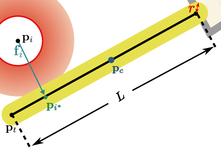
Figure 4: The nearest point on the capsule axis $\mathbf{p}_{i}^{*}$.

Given the length $L$ of the capsule axis which is a line segment, every point belonging to it is given by:

$$\mathbf{p}_{s}(\sigma;t)=\mathbf{p}_{t}(t)-\mathbf{n}_{t}L\sigma$$ (34)

with $\sigma\in[0,1]$. Then at every control cycle and for each point $\mathbf{p}_{i}\in\mathcal{O}_{s}$, we find the nearest point $\mathbf{p}{{}^{*}_{i}}=\mathbf{p}_{s}({\sigma}{{}^{*}_{i}},t)$ on the line segment of the capsule where ${\sigma}{{}^{*}_{i}}$ can be found analytically as described in our previous paper [33] :

$$\sigma{{}^{*}_{i}}=\begin{cases*}\zeta_{i},&\text{if $0\leq\zeta_{i}\leq 1$}\\ 1,&\text{if $\zeta_{i}>1$}\\ 0,&\text{if $\zeta_{i}<0$}\end{cases*}$$ (35)

where

$$\zeta_{i}=\dfrac{1}{L}\mathbf{n}_{t}^{\mathrm{T}}(\mathbf{p}_{t}-\mathbf{p}_{i}).$$

Then the barrier artificial potential $V_{i}(\mathbf{p}^{*}_{i})$ (9) can be applied for each pair $(\mathbf{p}_{i},\mathbf{p}^{*}_{i})$. Notice that in this case $d_{c}$ in (9) is replaced by $d_{c}+r$.

To impose actively the constraint for the capsule a repulsive force is applied at $\mathbf{p}^{*}_{i}$ calculated by the negative gradient of $V_{i}({\mathbf{p}^{*}_{i}})$, i.e., $\mathbf{f}_{i}(\mathbf{p}{{}^{*}_{i}})=-\dfrac{\partial V_{i}}{\partial\mathbf{p}{{}^{*}_{i}}}$ (11) for all points of the cloud. This is transformed in the tool-tip as a force $\mathbf{f}_{i}$ and a torque $\bm{\tau}_{i}$ given by:

$$\begin{bmatrix}{\mathbf{f}}_{i}\\ \bm{\tau}_{i}\end{bmatrix}=\begin{bmatrix}\ \ \ \ \mathbf{I}_{3\times 3}\ \ \ \ \ \mathbf{0}_{3\times 3}\\ (\mathbf{p}_{i}^{*}-\mathbf{p}_{t})^{\wedge}\ \ \mathbf{I}_{3\times 3}\end{bmatrix}\begin{bmatrix}{\mathbf{f}}_{i}\\ \mathbf{0}_{3\times 1}\end{bmatrix}.\in\mathbb{R}^{6\times 1},$$ (36)

The total generalized repulsive force on the tool-tip is given by the sum of the $\mathbf{f}_{i}$ forces and torques $\bm{\tau}_{i}$ produced by each artificial potential field i.e.,

$$\mathbf{F}_{r}=\sum_{\mathbf{p}_{i}\in\mathcal{O}_{s}}\begin{bmatrix}{\mathbf{f}}_{i}\\ {\bm{\tau}}_{i}\end{bmatrix}.$$ (37)

Then (37) is provided to the target admittance model (22). The proof of stability and enforcement of RCM and forbidden area constraints in this case is similar to the case of the tool-tip.

The proof of the first two statements of Theorem 1 are equivalent. To prove the third and fourth statement for the case of whole tool body constraint the following candidate Lyapunov is utilized:

$$V_{f}=\dfrac{1}{2}\dot{\mathbf{x}}_{f}^{\mathrm{T}}\dot{\mathbf{x}}_{f}+\sum_{\mathbf{p}_{i}\in\mathcal{O}_{s}}{V}_{i}({\mathbf{p}^{*}_{i}}).$$ (38)

Taking its time derivative yields:

$$\dot{V}_{f}=-\dot{\mathbf{x}}_{f}^{\mathrm{T}}\mathbf{D}_{f}\dot{\mathbf{x}}_{f}+\dot{\mathbf{x}}_{f}^{\mathrm{T}}\mathbf{Z}\mathbf{J}_{t}^{\mathrm{T}}\bigg{(}\mathbf{F}_{th}+{\mathbf{F}_{r}}\bigg{)}-\sum_{\mathbf{p}_{i}\in\mathcal{O}_{s}}\mathbf{f}_{i}(\mathbf{p}{{}^{*}_{i}})^{\mathrm{T}}\dot{\mathbf{p}}_{i}^{*}.$$ (39)

Furthermore, utilizing the time derivative of the nearest point $\dot{\mathbf{p}}_{i}^{*}=\begin{bmatrix}\ \mathbf{I}_{3\times 3}\ \ \ (\mathbf{p}_{t}-\mathbf{p}_{i}^{*})^{\wedge}\end{bmatrix}\mathbf{v}_{t}-\mathbf{n}_{t}L\dot{{\sigma}{{}^{*}_{i}}}$ in (39) yields:

$$\begin{split}\dot{V}_{f}=&-\dot{\mathbf{x}}_{f}^{\mathrm{T}}\mathbf{D}_{f}\dot{\mathbf{x}}_{f}+\dot{\mathbf{x}}_{f}^{\mathrm{T}}\mathbf{Z}\mathbf{J}_{t}^{\mathrm{T}}\bigg{(}\mathbf{F}_{th}+{\mathbf{F}_{r}}\bigg{)}+\sum_{\mathbf{p}_{i}\in\mathcal{O}_{s}}\mathbf{f}_{i}(\mathbf{p}{{}^{*}_{i}})^{\mathrm{T}}(\mathbf{n}_{t}L\dot{{\sigma}{{}^{*}_{i}}})\\ &-\sum_{\mathbf{p}_{i}\in\mathcal{O}_{s}}\mathbf{f}_{i}(\mathbf{p}{{}^{*}_{i}})^{\mathrm{T}}\begin{bmatrix}\ \mathbf{I}_{3\times 3}\ \ \ (\mathbf{p}_{t}-\mathbf{p}_{i}^{*})^{\wedge}\end{bmatrix}\mathbf{v}_{t}.\end{split}$$ (40)

Utilizing $\mathbf{F}_{r}$ from (37) and using (36) yields:

$$\begin{split}\dot{V}_{f}=&-\dot{\mathbf{x}}_{f}^{\mathrm{T}}\mathbf{D}_{f}\dot{\mathbf{x}}_{f}+\dot{\mathbf{x}}_{f}^{\mathrm{T}}\mathbf{Z}\mathbf{J}_{t}^{\mathrm{T}}\bigg{(}\mathbf{F}_{th}+{\mathbf{F}_{r}}\bigg{)}-{\mathbf{F}_{r}}^{\mathrm{T}}{\mathbf{v}}_{t}\\ &+\sum_{\mathbf{p}_{i}\in\mathcal{O}_{s}}\mathbf{f}_{i}(\mathbf{p}{{}^{*}_{i}})^{\mathrm{T}}(\mathbf{n}_{t}L\dot{{\sigma}{{}^{*}_{i}}}).\end{split}$$ (41)

For the first case of (35) utilizing (34) for $\sigma={\sigma}{{}^{*}_{i}}$ yields that $\mathbf{n}_{t}^{\mathrm{T}}(\mathbf{p}{{}^{*}_{i}}-\mathbf{p}_{i})=0$ and for the other two cases $\dot{\sigma}^{*}_{i}=0$. As $\mathbf{f}_{i}(\mathbf{p}{{}^{*}_{i}})$ is in the direction of $(\mathbf{p}{{}^{*}_{i}}-\mathbf{p}_{i})$ we get:

$$\begin{split}\dot{V}_{f}=&-\dot{\mathbf{x}}_{f}^{\mathrm{T}}\mathbf{D}_{f}\dot{\mathbf{x}}_{f}+\dot{\mathbf{x}}_{f}^{\mathrm{T}}\mathbf{Z}\mathbf{J}_{t}^{\mathrm{T}}\bigg{(}\mathbf{F}_{th}+{\mathbf{F}_{r}}\bigg{)}-{\mathbf{F}_{r}}^{\mathrm{T}}{\mathbf{v}}_{t}.\end{split}$$ (42)

The above equation is equivalent to (29) in the proof for the tool-tip case, thus the proof of the two last statements follows the same line.

4.4 Variable Damping

In order to facilitate kinesthetic guidance variable damping gains have been proposed in the literature [38]. In our case, the need for variable damping is more acute, as near the forbidden areas the manipulation performance of the tool is affected by the non-linear increase of the apparent stiffness induced by the artificial potentials. In order to achieve the objective of smooth performance in the whole of the tool’s workspace we utilize variable damping gains. In particular, the following variable damping gains are utilized in $\mathbf{D}_{f}\in\mathbb{R}^{(n-2)\times(n-2)}$:

$$\mathrm{D}_{f_{i}}=\mathrm{D}_{c_{i}}+\mathrm{D}_{v_{i}}+\mathrm{D}_{r_{i}},\ \ i=1,...,n-2$$ (43)

where $\mathrm{D}_{c_{i}}$ are positive constant values given for $i=1,...,(n-2)$ and $\mathrm{D}_{v_{i}}$ and $\mathrm{D}_{r_{i}}$ are variable damping terms added in the first four diagonal elements to facilitate motion along the task unconstrained coordinates. The term $\mathrm{D}_{v_{i}}$ is inspired by [38] and is given by :

$$\mathrm{D}_{v_{i}}=\begin{cases*}\mathrm{Q}_{i}exp(-\mathrm{M}_{i}s_{i}),&\text{for $i=1,...,4$}\\ 0,&\text{for $i=5,...,n-2$}\end{cases*}$$ (44)

where $\mathrm{Q}_{i}$ and $\mathrm{M}_{i}$ are positive constant gains, $s_{1}=|\dot{x}_{f_{1}}|$ and $s_{j}=||\dot{\mathbf{x}}_{f\{2:4\}}||$ for $j=2,3,4$. This exponential term provides high damping at low velocities and low damping for high velocities (see Fig 5 a) in order to facilitate the user to easily displace the tool in free space. The term $\mathrm{D}_{r_{i}}$ serves to enhance the protection of the forbidden region and the feeling of control over the task within the range of influence of the repulsive field. It provides increased damping as the virtual stiffness induced by the artificial potential increases. Thus unwanted oscillatory motion is avoided. The term $\mathrm{D}_{r_{i}}$ is given by:

$$\mathrm{D}_{r_{i}}=\begin{cases*}\mathrm{G}_{i}(1-exp(-\mathrm{C}_{i}z_{i}^{2})),&\text{for $i=1,...,4$}\\ 0,&\text{for $i=5,...,n-2$}\end{cases*}$$ (45)

where $\mathrm{C}_{i},\ \mathrm{G}_{i}$ are constant gains, $z_{1}=|F_{rx\{1\}}|$ and $z_{j}=||{\mathbf{F}}_{rx\{2:4\}}||$ for $j=2,3,4$ where $\mathbf{F}_{rx}=\mathbf{Z}_{x}^{\mathrm{T}}\mathbf{F}_{r}$. This term utilizes the magnitude of the repulsive force along the tool axis and the magnitude of repulsive torques. It increases the damping when these forces are high and is zero beyond the influence region. (see Fig 5 b). Notice that $\mathrm{D}_{v_{i}}$ and $\mathrm{D}_{r_{i}}$ are bounded non-negative functions thus they do not affect the stability proof.

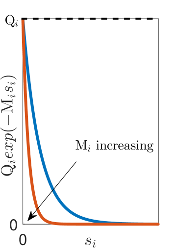
(a) The velocity-dependent term $\mathrm{D}_{v_{i}}$

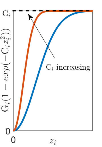
(b) The term $\mathrm{D}_{r_{i}}$ depending on the repulsive force

Figure 5: The variable damping terms.

5 Experimental results

In order to validate the effectiveness and performance of the proposed target admittance model, a 7-dof KUKA LWR4+ robotic manipulator with a force/torque sensor (ATI Mini40) attached at its end-effector is used in joint position control mode. This mode of operation provides a high bandwidth control of the robot dynamics so that the desired joint motion $\mathbf{q}_{d}$ from (22) is faithfully tracked. Hence, approximately $\mathbf{q}=\mathbf{q}_{d}$. The set-up is mimicking a hands-on surgical procedure. In particular, the robot holds a tool of length $0.43\ m$ and diameter $7\ mm$, mimicking a surgical instrument in a real RAMIS procedure. Typically the diameter of a surgical instrument is in the range of 3-12 mm. The entry port, imitating the incision point on the patients body wall, is a ring softly attached to the environment with the position of its center being $\mathbf{p}_{c}=[-0.6053\ \ -0.2203\ \ 0]^{\mathrm{T}}\ m$. The initial joint configuration is $\mathbf{q}_{d}(0)=[20\ 50\ 0\ -70\ 0\ 60\ 0]^{\mathrm{T}}\ deg$ so that the tool passes through the central point of the ring (Figure 6). In a real surgical procedure its position can be found utilizing the robot [39], [40], [41] or camera images from the external surgical scene [42].

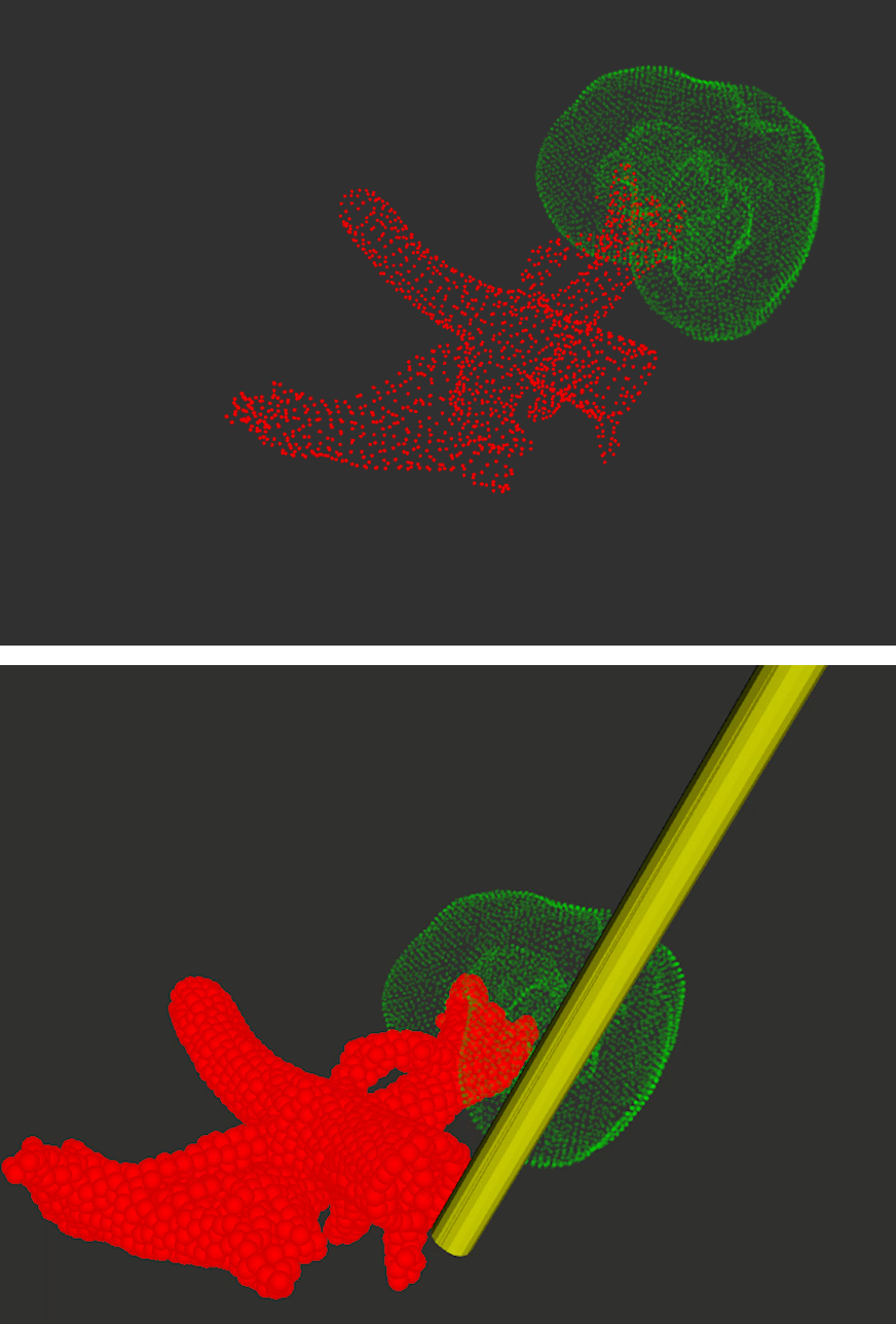
(a)

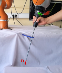
(b)

Figure 6: Experimental setup: (a) Visualization of the point cloud of a kidney (green) and its surrounding vessels (red) as the forbidden one with the overlapping spheres of the forbidden region shown in the bottom. (b) The robot holds a long tool mimicking a surgical instrument in a real RAMIS hands-on procedure.

Table 1: Parameters of the proposed method.

$\mathbf{W}$	$\alpha,\ \beta$	$\mathrm{d}_{0}$	$\mathrm{k}_{i}$
$1.5\mathrm{I}_{7\times 7}$	$25$	$0.0115\ m$	$0.01$

Parameters for the variable Damping matrix $\mathbf{D}_{f}$
Element $i$	$\mathrm{D}_{c_{i}}$	$\mathrm{Q}_{i}$	$\mathrm{M}_{i}$	$\mathrm{G}_{i}$	$\mathrm{C}_{i}$
$1$	10	25	22	60	0.01
$\{2:4\}$	4	20	19	30	0.2
$5$	60	-	-	-	-

The point cloud of an internal human organ (kidney with green points) and its surrounding vessels (red points) is imported in the robot’s workspace (Figure 6). The task is to manipulate the tool in the surgical area of the kidney avoiding the sensitive region of the surrounding vessels. After down sampling the point cloud of the vessels to increase computational performance, the radius of the spheres to cover the empty spaces is calculated to be $\mathrm{d}_{c}=3.5mm$. In the real case the 3D point cloud of the surgical site will be provided by the endoscopic camera and the characterization of the forbidden areas can be performed by the surgeon via a friendly human machine interface. For providing visual feedback to the user, a virtual scene, displaying the point cloud of the surgical site and the virtual timestamp of the real robot with the tool, is created utilizing Rviz embedded in ROS framework (Figure 6). The whole scheme is implemented in C++ with control frequency $\mathrm{f_{s}}=250$ using the Fast Research Interface (FRI) library. The FRI library is provided by the manufacturer and allows the communication between the KUKA LWR4+ Robot’s Controller (KRC) and a remote PC over the Ethernet [43]. The target admittance model (22) with the parameters values given in table 1 is integrated every 4ms using the Euler method and the derivative of the matrix $\mathbf{A}$ used in the model is numerically calculated using the backward differentiation formula.

For the experimental evaluation, the user was asked to guide the tool on the surgical area and towards the sensitive region entering the region of active constraints influence. Experiments demonstrate RCM manipulation and that the forbidden region is never violated by the tool tip (first experiment) and by the whole tool (scecond experiment).

5.1 Tool-tip case

The user guides the tool-tip initially on the surgical area and then approaches the sensitive region (vessels) entering the region of the active constraints influence. Experimental results are presented in Figure 7.

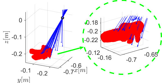
(a) Traces of the tool axis

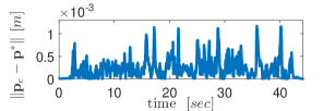
(b) The minimum distance between $\mathbf{p}_{c}$ and the tool axis $\mathbf{n}$ where $\mathbf{p}^{*}=\mathbf{p}+\mathbf{n}\mathbf{n}^{\mathrm{T}}(\mathbf{p}_{c}-\mathbf{p})$.

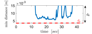
(c) The minimum distance between the tip of the tool and the point cloud of the sensitive area.

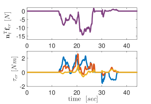
(d) Repulsive forces and torques.

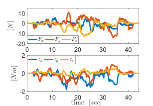
(e) Human force and torque.

Figure 7: Experimental results: case of tool-tip constraint.

Human exerted forces and torques are shown Figure 7-e. After $t_{1}$=12.5 sec the user has guided the tool-tip at a distance less than $d_{0}+d_{c}=0.015m$ from the vessels triggering the generation of repulsive forces at the tip. Figure 7-d shows repulsive forces and torques acting on the entry port i.e. $\mathbf{n}_{t}^{\mathrm{T}}{\mathbf{f}}_{cr}$ and ${\bm{\tau}}_{cr}$ respectively where $\begin{bmatrix}{\mathbf{f}}_{cr}\\ \bm{\tau}_{cr}\end{bmatrix}=\begin{bmatrix}\ \ \ \ \mathbf{I}_{3\times 3}\ \ \ \ \ \mathbf{0}_{3\times 3}\\ (\mathbf{p}_{t}-\mathbf{p}_{c})^{\wedge}\ \ \mathbf{I}_{3\times 3}\end{bmatrix}\mathbf{F}_{r}\in\mathbb{R}^{6\times 1}$. These forces actively resist the user for damaging the sensitive region with the tool tip. This is confirmed by the tip distance from the forbidden area shown in Figure 7-c after $t_{1}$=19 sec which remains greater than $d_{c}$. Figure 7-a shows the traces of the tool during the manipulation. Clearly, the desired RCM constraint is satisfied as also shown in Figure 7-b by the minimum distance between the incision point $\mathbf{p}_{c}$ and the axis of the tool, $\mathbf{n}$ which is kept less than $1.2mm$; ideally this distance should stay within the range of displacement $\mathbf{x}_{c}$ in the constraint space whose norm is shown in Figure 8 and is in the order of $10^{-6}m$. The higher displacement $1.2mm$ in the experiment can be attributed to the fact that the controlled robot is not infinitely stiff hence robot joint positions are approximately equal but not identical to the provided reference values. Clearly the controlled robot stiffness affects the magnitude of errors we get regarding the satisfaction of the desired RCM constraint. In Figure 7-a the embedded subplot shows details of the tool traces where it can be observed that part of the tool are in some instances inside the forbidden area. This is expected as in this experiment the avoidance concerns only the tool tip.

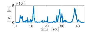
(a)

Figure 8: The norm of the desired position constraint $||\mathbf{x}_{c}||$.

Figure 9 shows the varying damping gains during the experiment. $\mathrm{D}_{v_{i}}$ are shown in blue and $\mathrm{D}_{r_{i}}$ in red. Notice in the beginning and in the end of the motion the terms $\mathrm{D}_{v_{i}}$ that have maximum value as there is zero velocity. Further notice how $\mathrm{D}_{r_{i}}$ take non-zero values when entering the region of influence of the repulsive potential and how they increase when respective repulsive force/torques increase.

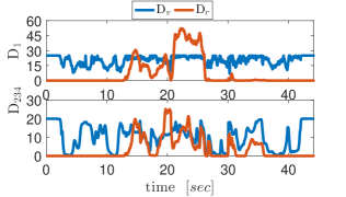
(a)

Figure 9: Damping gain variation during the experiment.

5.2 Whole tool case

A capsule with radius $\mathrm{r}=3.5mm$ encloses the elongated tool. As in the previous case the user guides the tool towards to the sensitive region (vessels) entering the region of the active constraints influence. Experimental results are presented in Figure 10. Human exerted forces and torques are shown in Figure 10-e. Notice that the user applied forces of magnitude close to 30 N, with the system responding in a stable smooth manner. Such large forces were exerted on purpose close to the forbidden areas to investigate the controller’s performance but much smaller forces are adequate during surgery. After $t_{1}=13$ sec the user has guided the tool at a distance less than $d_{0}+d_{c}+r=0.0185m$ from the vessels triggering the generation of repulsive forces and torques shown in Figure 10-d that actively resist the user for damaging the sensitive region as shown by the minimum tool distance from the forbidden area (Figure 10-c after $t_{1}=13$ sec) which remains greater than $d_{c}+r$. Figure 10-a shows the traces of the tool during the manipulation. Clearly, the desired RCM constraint is satisfied as also shown in Figure 10-b by the minimum distance between the incision point $\mathbf{p}_{c}$ and the axis of the tool, $\mathbf{n}$ which is kept less than 1.1mm as shown in Figure 10-b. In Figure 10-a the embedded subplot shows details of the tool traces where it can be observed that the whole tool never violates the forbidden area as expected . Figure 11 shows the varying damping gains. The video of the experiment can be seen in: $https://youtu.be/NB1x8WzwbOQ$.

The proposed admittance control scheme have been validated via experiments involving tools with different lengths. We expected that the parameter values of $G_{i}$ and $C_{i},i=\{2:4\}$ involved in the variable damping term $\mathbf{D}_{f}$ may need to be adjusted because the torques induced on the RCM by the repulsive forces are amplified in the case of longer instruments. However, keeping the same control parameter values we found that the performance was satisfactory when the tool length was in the range of 30 cm to 43 cm.

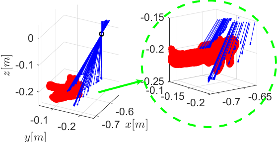
(a) Traces of the tool axis.

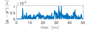
(b) The minimum distance between $\mathbf{p}_{c}$ and the tool axis $\mathbf{n}$ where $\mathbf{p}^{*}=\mathbf{p}+\mathbf{n}\mathbf{n}^{\mathrm{T}}(\mathbf{p}_{c}-\mathbf{p})$.

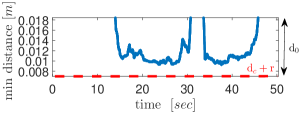
(c) The minimum distance between the tool axis and the point cloud of the sensitive area.

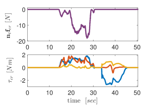
(d) Repulsive forces and torques.

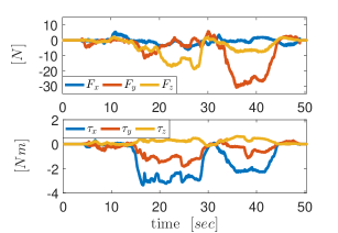
(e) Human force and torque.

Figure 10: Experimental results: case of whole tool constraint.

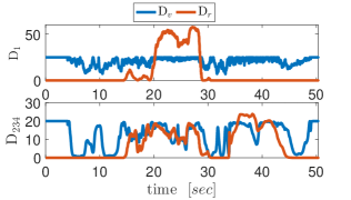
(a)

Figure 11: Damping gain variation during the experiment.

6 Conclusions

This paper proposes a passive admittance controller achieving RCM and spatial constraint satisfaction to guarantee the safety of sensitive regions. The admittance model is designed in such a way so that the control action that guarantees manipulation away from the spatial constraints does not affect the satisfaction of the RCM constraint and vice versa. Moreover, it provides manipulation transparency and smooth motion even close to the forbidden regions enhancing the user’s sense of control over the task. Experimental results on 7-dof KUKA LWR4+ robot manipulator simulating a real minimally invasive surgery procedure demonstrate the efficacy of the proposed scheme. The whole tool never touches the forbidden region and tool manipulation via a RCM is achieved in a intuitive manner. Future work focus on adapting the proposed method for a tele-operated setup and testing it in a real surgical environment.

References

- Khatib [1980] O. Khatib, Commande dynamique dans l’espace opérationnel des robots manipulateurs en présence d’obstacles, PhD dissertation, Ecole Nationale Superieure de l’Aeronautique et de l’Espace (1980).
- Papageorgiou et al. [2020] D. Papageorgiou, T. Kastritsi, Z. Doulgeri, G. A. Rovithakis, A passive phri controller for assisting the user in partially known tasks, IEEE Transactions on Robotics 36 (2020) 802–815.
- Theodorakopoulos et al. [2015] A. Theodorakopoulos, G. A. Rovithakis, Z. Doulgeri, An impedance control modification guaranteeing compliance strictly within preselected spatial limits, in: 2015 IEEE/RSJ International Conference on Intelligent Robots and Systems (IROS), IEEE, pp. 2210–2215.
- Bettini et al. [2002] A. Bettini, S. Lang, A. Okamura, G. Hager, Vision assisted control for manipulation using virtual fixtures: Experiments at macro and micro scales, in: Proceedings 2002 IEEE International Conference on Robotics and Automation (Cat. No. 02CH37292), volume 4, IEEE, pp. 3354–3361.
- Bettini et al. [2004] A. Bettini, P. Marayong, S. Lang, A. M. Okamura, G. D. Hager, Vision-assisted control for manipulation using virtual fixtures, IEEE Transactions on Robotics 20 (2004) 953–966.
- Bowyer and y Baena [2015] S. A. Bowyer, F. R. y Baena, Dissipative control for physical human–robot interaction, IEEE Transactions on Robotics 31 (2015) 1281–1293.
- Papageorgiou et al. [2020a] D. Papageorgiou, F. Dimeas, T. Kastritsi, Z. Doulgeri, Kinesthetic guidance utilizing dmp synchronization and assistive virtual fixtures for progressive automation, Robotica 38 (2020a) 1824–1841.
- Papageorgiou et al. [2020b] D. Papageorgiou, T. Kastritsi, Z. Doulgeri, A passive robot controller aiding human coaching for kinematic behavior modifications, Robotics and Computer-Integrated Manufacturing 61 (2020b) 101824.
- Kastritsi et al. [2019] T. Kastritsi, D. Papageorgiou, I. Sarantopoulos, S. Stavridis, Z. Doulgeri, G. A. Rovithakis, Guaranteed active constraints enforcement on point cloud-approximated regions for surgical applications, in: 2019 International Conference on Robotics and Automation (ICRA), IEEE, pp. 8346–8352.
- Rydén and Chizeck [2012] F. Rydén, H. J. Chizeck, Forbidden-region virtual fixtures from streaming point clouds: Remotely touching and protecting a beating heart, in: 2012 IEEE/RSJ International Conference on Intelligent Robots and Systems, IEEE, pp. 3308–3313.
- Rydén et al. [2013] F. Rydén, A. Stewart, H. J. Chizeck, Advanced telerobotic underwater manipulation using virtual fixtures and haptic rendering, in: 2013 OCEANS-San Diego, IEEE, pp. 1–8.
- Leibrandt et al. [2014] K. Leibrandt, H. J. Marcus, K.-W. Kwok, G.-Z. Yang, Implicit active constraints for a compliant surgical manipulator, in: 2014 IEEE International Conference on Robotics and Automation (ICRA), IEEE, pp. 276–283.
- Kastritsi and Doulgeri [2020] T. Kastritsi, Z. Doulgeri, Human-guided desired rcm constraint manipulation with applications in robotic surgery: A torque level control approach., in: 2020 European Control Conference (ECC), IEEE, pp. 1448–1453.
- Kastritsi and Doulgeri [2021] T. Kastritsi, Z. Doulgeri, A controller to impose a rcm for hands-on robotic-assisted minimally invasive surgery, IEEE Transactions on Medical Robotics and Bionics 3 (2021) 392–401.
- Sandoval et al. [2018a] J. Sandoval, H. Su, P. Vieyres, G. Poisson, G. Ferrigno, E. D. Momi, Collaborative framework for robot-assisted minimally invasive surgery using a 7-dof anthropomorphic robot, Robotics and Autonomous Systems 106 (2018a) 95 – 106.
- Sandoval et al. [2018b] J. Sandoval, P. Vieyres, G. Poisson, Generalized framework for control of redundant manipulators in robot-assisted minimally invasive surgery, IRBM 39 (2018b) 160–166.
- Su et al. [2019] H. Su, C. Yang, G. Ferrigno, E. De Momi, Improved human–robot collaborative control of redundant robot for teleoperated minimally invasive surgery, IEEE Robotics and Automation Letters 4 (2019) 1447–1453.
- Azimian et al. [2010] H. Azimian, R. V. Patel, M. D. Naish, On constrained manipulation in robotics-assisted minimally invasive surgery, in: 2010 3rd IEEE RAS EMBS International Conference on Biomedical Robotics and Biomechatronics, pp. 650–655.
- Yang et al. [2019] B. Yang, W. Chen, Z. Wang, Y. Lu, J. Mao, H. Wang, Y.-H. Liu, Adaptive fov control of laparoscopes with programmable composed constraints, IEEE Transactions on Medical Robotics and Bionics 1 (2019) 206–217.
- Sadeghian et al. [2019] H. Sadeghian, F. Zokaei, S. H. Jazi, Constrained kinematic control in minimally invasive robotic surgery subject to remote center of motion constraint, Journal of Intelligent & Robotic Systems 95 (2019) 901–913.
- He et al. [2021] Y. He, B. Zhao, X. Qi, S. Li, Y. Yang, Y. Hu, Automatic surgical field of view control in robot-assisted nasal surgery, IEEE Robotics and Automation Letters 6 (2021) 247–254.
- Aghakhani et al. [2013] N. Aghakhani, M. Geravand, N. Shahriari, M. Vendittelli, G. Oriolo, Task control with remote center of motion constraint for minimally invasive robotic surgery, in: 2013 IEEE International Conference on Robotics and Automation, pp. 5807–5812.
- Boctor et al. [2004] E. M. Boctor, R. J. Webster III, H. Mathieu, A. M. Okamura, G. Fichtinger, Virtual remote center of motion control for needle placement robots, Computer Aided Surgery 9 (2004) 175–183.
- Pham et al. [2015] C. D. Pham, F. Coutinho, A. C. Leite, F. Lizarralde, P. J. From, R. Johansson, Analysis of a moving remote center of motion for robotics-assisted minimally invasive surgery, in: 2015 IEEE/RSJ International Conference on Intelligent Robots and Systems (IROS), IEEE, pp. 1440–1446.
- Kapoor et al. [2006] A. Kapoor, M. Li, R. H. Taylor, Constrained control for surgical assistant robots., in: ICRA, pp. 231–236.
- He et al. [2014] X. He, M. Balicki, P. Gehlbach, J. Handa, R. Taylor, I. Iordachita, A multi-function force sensing instrument for variable admittance robot control in retinal microsurgery, in: 2014 IEEE International Conference on Robotics and Automation (ICRA), IEEE, pp. 1411–1418.
- Rosenberg [1992] L. B. Rosenberg, The Use of Virtual Fixtures as Perceptual Overlays to Enhance Operator Performance in Remote Environments., Technical Report, Stanford Univ Ca Center for Design Research, 1992.
- Rosenberg [1993] L. B. Rosenberg, Virtual fixtures: Perceptual tools for telerobotic manipulation, in: Proceedings of IEEE virtual reality annual international symposium, IEEE, pp. 76–82.
- Moccia et al. [2019] R. Moccia, M. Selvaggio, L. Villani, B. Siciliano, F. Ficuciello, Vision-based virtual fixtures generation for robotic-assisted polyp dissection procedures, in: 2019 IEEE/RSJ International Conference on Intelligent Robots and Systems (IROS), IEEE, pp. 7934–7939.
- Petersen and Baena [2013] J. G. Petersen, F. R. Baena, A dynamic active constraints approach for hands-on robotic surgery, in: 2013 IEEE/RSJ International Conference on Intelligent Robots and Systems, IEEE, pp. 1966–1971.
- Colgate et al. [2003] J. E. Colgate, M. Peshkin, S. H. Klostermeyer, Intelligent assist devices in industrial applications: a review, in: Proceedings 2003 IEEE/RSJ International Conference on Intelligent Robots and Systems (IROS 2003)(Cat. No. 03CH37453), volume 3, IEEE, pp. 2516–2521.
- Lin et al. [2006] H. C. Lin, K. Mills, P. Kazanzides, G. D. Hager, P. Marayong, A. M. Okamura, R. Karam, Portability and applicability of virtual fixtures across medical and manufacturing tasks, in: Proceedings 2006 IEEE International Conference on Robotics and Automation, 2006. ICRA 2006., IEEE, pp. 225–230.
- Kastritsi et al. [2019] T. Kastritsi, I. Sarantopoulos, S. Stavridis, D. Papageorgiou, Z. Doulgeri, Manipulation of a whole surgical tool within safe regions utilizing barrier artificial potentials, in: Mediterranean Conference on Medical and Biological Engineering and Computing, Springer, pp. 1559–1570.
- Bowyer et al. [2013] S. A. Bowyer, B. L. Davies, F. R. y Baena, Active constraints/virtual fixtures: A survey, IEEE Transactions on Robotics 30 (2013) 138–157.
- Lamy et al. [2009] X. Lamy, F. Colledani, F. Geffard, Y. Measson, G. Morel, Achieving efficient and stable comanipulation through adaptation to changes in human arm impedance, in: 2009 IEEE International Conference on Robotics and Automation, IEEE, pp. 265–271.
- Ott [2008] C. Ott, Cartesian impedance control of redundant and flexible-joint robots, Springer, 2008.
- Park et al. [1999] J. Park, W. Chung, Y. Youm, On dynamical decoupling of kinematically redundant manipulators, in: Proceedings 1999 IEEE/RSJ International Conference on Intelligent Robots and Systems. Human and Environment Friendly Robots with High Intelligence and Emotional Quotients (Cat. No. 99CH36289), volume 3, IEEE, pp. 1495–1500.
- Ficuciello et al. [2015] F. Ficuciello, L. Villani, B. Siciliano, Variable impedance control of redundant manipulators for intuitive human–robot physical interaction, IEEE Transactions on Robotics 31 (2015) 850–863.
- Ortmaier and Hirzinger [2000] T. Ortmaier, G. Hirzinger, Cartesian control issues for minimally invasive robot surgery, in: Proceedings. 2000 IEEE/RSJ International Conference on Intelligent Robots and Systems (IROS 2000) (Cat. No.00CH37113), volume 1, pp. 565–571 vol.1.
- Lin Dong and Morel [2016] Lin Dong, G. Morel, Robust trocar detection and localization during robot-assisted endoscopic surgery, in: 2016 IEEE International Conference on Robotics and Automation (ICRA), pp. 4109–4114.
- Gruijthuijsen et al. [2018] C. Gruijthuijsen, L. Dong, G. Morel, E. V. Poorten, Leveraging the fulcrum point in robotic minimally invasive surgery, IEEE Robotics and Automation Letters 3 (2018) 2071–2078.
- Rosa et al. [2015] B. Rosa, C. Gruijthuijsen, B. Van Cleynenbreugel, J. V. Sloten, D. Reynaerts, E. V. Poorten, Estimation of optimal pivot point for remote center of motion alignment in surgery, International Journal of Computer Assisted Radiology and Surgery 10 (2015) 205–215.
- Schreiber et al. [2010] G. Schreiber, A. Stemmer, R. Bischoff, The fast research interface for the kuka lightweight robot, in: IEEE workshop on innovative robot control architectures for demanding (Research) applications how to modify and enhance commercial controllers (ICRA 2010), Citeseer, pp. 15–21.