North Ecliptic Pole merging galaxy catalogue

Abstract

Aims. We aim to generate a catalogue of merging galaxies within the 5.4 sq. deg. North Ecliptic Pole over the redshift range $0.0<z<0.3$. To do this, imaging data from the Hyper Suprime-Cam are used along with morphological parameters derived from these same data.

Methods. The catalogue was generated using a hybrid approach. Two neural networks were trained to perform binary merger non-merger classifications: one for galaxies with $z<0.15$ and another for $0.15\leq z<0.30$. Each network used the image and morphological parameters of a galaxy as input. The galaxies that were identified as merger candidates by the network were then visually checked by experts. The resulting mergers will be used to calculate the merger fraction as a function of redshift and compared with literature results.

Results. We found that 86.3% of galaxy mergers at $z<0.15$ and 79.0% of mergers at $0.15\leq z<0.30$ are expected to be correctly identified by the networks. Of the 34 264 galaxies classified by the neural networks, 10 195 were found to be merger candidates. Of these, 2109 were visually identified to be merging galaxies. We find that the merger fraction increases with redshift, consistent with literature results from observations and simulations, and that there is a mild star-formation rate enhancement in the merger population of a factor of $1.102\pm 0.084$.

1 Introduction

Galaxy mergers underpin our current understanding of how galaxies grow and evolve. In the current cold dark matter paradigm, dark matter halos assemble hierarchically. This results in the baryonic constituents of the dark matter halos also merging. The result is a larger galaxy living in the heart of a larger dark matter halo (e.g. Conselice 2014; Somerville & Davé 2015).

Numerous studies have looked at how galaxy-galaxy mergers influence the star-formation rate (SFR) or active galactic nuclei (AGN) activity of both the progenitor and descendant galaxies. The merger and SFR connection was raised when early infrared observations found that the majority of infrared-bright galaxies were merging. The link between infrared-bright galaxies and high SFRs resulted in the conclusion that galaxy mergers can trigger periods of highly enhanced SFRs and starbursts (e.g. Joseph & Wright 1985; Sanders & Mirabel 1996; Niemi et al. 2012). The increase in SFRs during a merger event has been seen in more recent works, although not all galaxy mergers are seen with highly enhanced SFRs that would be considered starbursts.

The constituent galaxies of a merger are found to play a role in the strength of star-formation enhancement. Interactions between two spiral galaxies have been shown to have an enhanced SFR, when compared to non-mergers, while little enhancement is seen when at least one of the merging galaxies is elliptical (Hwang et al. 2011). The strength of the interaction also influences star-formation, with galaxies whose projected distance to the nearest neighbour is less than a tenth of the virial radius of the nearest neighbour experiencing greater increases in specific SFRs, up to a factor of 4 (Hwang et al. 2011). Post-merger galaxies are also seen to have their SFR increase by a factor of approximately 4 when compared to a non-merging control sample (Ellison et al. 2013). The mass of the interacting galaxies is also likely to contribute to the star-formation enhancement, with galaxies with stellar masses below 10¹¹ M_⊙ showing a greater enhancement than more massive mergers. Indeed, major mergers of dwarf galaxies are found to have similar star-formation enhancement to more massive major mergers (Stierwalt et al. 2015).

Other studies have found weaker enhancement in star-formation during a merger. In Knapen et al. (2015), galaxy mergers are found to typically show mild star-formation enhancement, a factor of approximately 1.9 at most, with many merging systems showing no enhancement. These enhancements, or lack thereof, were determined by dividing the SFR of a merging system with the median SFR of that system’s control group. Similarly, Pearson et al. (2019a) also found mild enhancement, with the average SFR in mergers to be only a factor of 1.2 higher than the average SFR in non-mergers. However, the Pearson et al. (2019a) merger sample is likely to be highly contaminated by non-mergers due to their selection from only a neural network. Reductions in SFRs during galaxy mergers can be seen in low mass (stellar mass $<10^{9}$ M_⊙) secondary galaxies of minor mergers (Davies et al. 2015, 2016). Many dwarf starbursts, such as blue compact dwarf galaxies, appear to be a consequence of the strong interactions or mergers of even smaller entities. However, these features are only observed when deep images and complementary spectroscopic and/or radio data are available (López-Sánchez 2010; Martínez-Delgado et al. 2012; Zhang et al. 2020). What merger studies do agree on, however, is that not all galaxy mergers are undergoing a starburst at the time of observation but starbursts are more common in mergers than non-mergers (Ellison et al. 2008; Hwang et al. 2011; Scudder et al. 2012; Ellison et al. 2013; Patton et al. 2013; Knapen et al. 2015; Stierwalt et al. 2015; Pearson et al. 2019a).

These observational findings agree with what is seen in simulations. Zoom-in simulations of merging galaxies allow the SFR to be closely tracked during an entire simulated merger with fine time-resolution. Such simulations indicate that galaxies go through short periods of highly enhanced star-formation (e.g. Cox et al. 2006; Bournaud et al. 2011; Hopkins et al. 2013; Bournaud et al. 2015; Sparre & Springel 2016; Moreno et al. 2019; Rodríguez Montero et al. 2019). These are typically seen around first close passage and coalescence of the merging galaxies. Thus, only short periods of a galaxy merger are able to be observed to have highly enhanced SFRs resulting in real galaxies typically being observed while only experiencing mild SFR enhancement.

Integral field observations have allowed resolved star-formation, rather than global star-formation, to be traced in mergers. With such observations, the merger triggered star-formation has been seen to primarily occur in the centre of a galaxy while the outer regions of the interacting galaxies show enhancement or suppression (Thorp et al. 2019), with the enhancement or suppression being dependent on the merger period (Pan et al. 2019).

High infrared emission can also be linked with AGN activity, where the AGN are known to heat the dust that surrounds them, emitting strongly in the infrared. Galaxy mergers have been seen to drive material onto a central black hole of a galaxy, feeding the AGN and resulting in increased activity (e.g. Keel et al. 1985; Silverman et al. 2011; Hwang et al. 2012; Lackner et al. 2014; Satyapal et al. 2014; Scott & Kaviraj 2014; Weston et al. 2017; Goulding et al. 2018; Ellison et al. 2019; Gao et al. 2020). However, this interpretation is contested, with a number of studies finding similar fractions of AGN in and out of galaxy mergers (e.g. Kocevski et al. 2012; Mechtley et al. 2016; Silva et al. 2021). This contention may be due to differences in the type of selected AGN (e.g. obscured or unobscured; Koss et al. 2010; Kocevski et al. 2015) or differing merger identification methods (Lambrides et al. 2021).

The merger rate and fraction in the Universe is not constant with redshift. Both observations and simulations typically agree that the fraction and rate of galaxy mergers was higher in the earlier Universe and has decreased as the Universe has aged (e.g. Patton et al. 2002; Lin et al. 2004; Kartaltepe et al. 2007; de Ravel et al. 2009; Lotz et al. 2011; Cotini et al. 2013; López-Sanjuan et al. 2013; Casteels et al. 2014; Rodriguez-Gomez et al. 2015; Mundy et al. 2017; Qu et al. 2017; Moster et al. 2018; Duncan et al. 2019; Pearson et al. 2019a; Ferreira et al. 2020; O’Leary et al. 2021). The observationally determined merger fraction and rate evolutions use different selection methods, providing a firm determination of the increase of these two values with redshift. However, the exact evolution of the merger fraction and merger rate differ between different studies. Indeed, the simulations also do not agree on the evolution of these two quantities. The Horizon-AGN cosmological simulation (Dubois et al. 2014) finds no evolution of the merger fraction with redshift (Kaviraj et al. 2015), unlike other simulations that find an increase with redshift (Rodriguez-Gomez et al. 2015; Qu et al. 2017). There is also observational evidence that the merger fraction may reduce above $z\approx 2$ for intermediate mass galaxies (M_⋆ between 10⁹ and 10¹⁰ M_⊙ Conselice et al. 2008). The difference in the evolution of the merger rate when compared to the evolution of the merger fraction may be resolved by using an evolving merger timescale instead of a fixed merger timescale (Snyder et al. 2017).

Merging galaxies are traditionally selected by identifying close pairs, that is finding galaxies that are close both on the sky and in redshift (e.g. Barton et al. 2000; De Propris et al. 2005; Robotham et al. 2014; Rodrigues et al. 2018; Duncan et al. 2019), or morphologically disturbed systems, identified either visually or through parametric and non-parametric statistics (e.g. Bershady et al. 2000; Conselice et al. 2000, 2003; Lintott et al. 2008, Kim et al. in Prep). For the latter technique, the majority of mergers are only identifiable for part of the merger time (Lotz et al. 2010a, b) and any study of merger rates or fractions with such identifications assumes that the scatter into and out of the selection is approximately equal. Visual selection, in particular, is a time intensive task which limits the sample size of merging galaxies that can be identified while the classifications can be difficult to reproduce and can be incomplete (Huertas-Company et al. 2015). This visual selection is also biased towards mergers that are closer to a pericentric passage where the morphological disturbance caused by the interaction is more visible (e.g. Blumenthal et al. 2020). More recent developments have allowed the detection of merging galaxies using machine learning which is orders of magnitude faster than visual selection (e.g. Ackermann et al. 2018; Bottrell et al. 2019; Nevin et al. 2019; Pearson et al. 2019a, b; Walmsley et al. 2019; Ferreira et al. 2020; Wang et al. 2020). However, such identifications are known to suffer from impurity of the merger sample (e.g. as shown by Bickley et al. 2021) and are limited by the quality of the training sample. Here we aim to obtain a clean sample of merging systems which will allow detailed follow-up studies of a statistically large number of galaxy mergers. Thus, we combine the speed of machine learning identification with a accuracy of visual classification.

This paper presents a large catalogue of merging galaxies with redshifts between 0.0 and 0.3 that is ideally suited for studying the link between merging galaxies and rarer astrophysical phenomena, such as AGN. The presented catalogue is for galaxies within the North Ecliptic Pole (NEP), a 5.4 sq. deg. area that has been well studied in numerous wavelength ranges (Kim et al. 2021), including infrared data from AKARI (Murakami et al. 2007; Kim et al. 2012), optical data from the Hyper Suprime-Cam (HSC; Goto et al. 2017; Furusawa et al. 2018; Kawanomoto et al. 2018; Komiyama et al. 2018; Miyazaki et al. 2018; Oi et al. 2021) and X-ray data from Chandra (Krumpe et al. 2015). This allows for studies correlating galaxy mergers with rare phenomena to be undertaken. The NEP will also be used as the location for a deep Euclid field (Laureijs et al. 2011). Thus the objects within the catalogue will have high quality near-infrared images taken in the near future. This catalogue will provide an excellent training sample for automated detection of further mergers throughout the Euclid coverage.

The catalogue presented in this work was generated using a hybrid deep learning - human approach, as proposed by Bickley et al. (2021). Deep learning techniques, applied to imaging and morphological data, were used to generate a sample of merger candidates. These merger candidates were then visually inspected by professional astronomers to create a final catalogue of galaxy mergers. The paper is structured as follows. Section 2 describes the data used to generate this catalogue. Section 3 discusses deep learning and the neural networks used to generate the merger candidates along with the human verification process. Section 4 presents the results of the merger identification and Sect. 5 presents discussion on these classifications. We summarise our work in Sect. 6.

2 Data

2.1 Imaging data

For the training data, we used imaging data from the HSC Subaru Strategic Program (HSC-SSP) Data Release 2 (DR2; Aihara et al. 2018, 2019). The galaxies used for training were selected using $r$-band data (see Sect. 2.3) and so HSC-SSP wide field $r$-band imaging was used. Within the HSC-SSP, the wide field $r$-band magnitude 5$\sigma$ limit is 26.2 AB mag. The morphological parameters were also derived from the $r$-band HSC-SSP data using statmorph (Rodriguez-Gomez et al. 2019).

For identifying galaxy mergers within NEP, HSC data from the HSC survey of NEP were used (HSC-NEP; Goto et al. 2017; Oi et al. 2021). Here we again used the $r$-band data, which reaches a median 5$\sigma$ depth of 27.3 AB mag, to match the band used for the training data. This choice of band is despite the HSC-NEP $r$-band having poorer seeing than other HSC-NEP optical bands: 1.26 arcsec in the $r$-band compared to 0.68 arcsec in the $g$-band (Oi et al. 2021). Galaxy positions and magnitudes were derived by Oi et al. (2021) using the HSC data analysis pipeline version 4.0.1 (Bosch et al. 2018). The photometric redshifts for the NEP galaxies were derived in Ho et al. (2021) using the Canada France Hawaii Telescope MegaPrime u-band (Boulade et al. 2003; Oi et al. 2014; Huang et al. 2020), HSC $g$, $r$, $i$, $z$, and $y$-bands, and the Spitzer Infrared Array Camera bands 1 and 2 (Fazio et al. 2004; Nayyeri et al. 2018) using LePhare (Arnouts et al. 1999; Ilbert et al. 2006). The photometric redshifts have a weighted dispersion of $\sigma_{\Delta z/(1+z)}=0.053$ and catastrophic error fraction of 11.3%. Spectroscopic redshifts were derived from optical spectroscopy (Shim et al. 2013; Oi et al. 2017; Kim et al. 2018; Ohyama et al. 2018). The galaxy sample that was checked for mergers were chosen where their photometric redshift, or spectroscopic redshift where available, is less than $z=0.30$. Above this redshift, the quality of the neural networks used to identify the galaxy mergers rapidly deteriorated. Of the 34 264 galaxies from HSC-NEP with $z<0.30$, 736 have spectroscopic redshifts and the remaining 33 528 have photometric redshifts. Morphological parameters were again derived using statmorph using the $r$-band images and segmentation maps were created using SExtractor (Bertin & Arnouts 1996).

2.2 Morphological parameters

To supplement the imaging data, morphological parameters of the galaxies were also used to help identify galaxy mergers. The morphological parameters used in this work were all derived from the HSC $r$-band images using the statmorph python package. These parameters are described below.

The concentration (C; Kent 1985; Abraham et al. 1994; Bershady et al. 2000; Conselice 2003) describes the ratio between amount of light towards the centre of a galaxy with the amount of light within a larger radius. The statmorph package follows Lotz et al. (2004) and compares the ratio of the radius that contains 20% of the light and the radius that contains 80% of the light. Larger values of C indicate that more light is concentrated in the centre of the galaxy.

The asymmetry (A; Abraham et al. 1996; Conselice et al. 2000) measures the rotational symmetry of a galaxy, the calculation of which again follows Lotz et al. (2004). An image is rotated by 180^∘ and this rotated image is subtracted from the original image. The residual values in the pixels are summed to give the final value of asymmetry. Larger values of asymmetry indicate that a galaxy is less rotationally symmetric.

The smoothness (S; Takamiya 1999; Conselice 2003) determination in statmorph follows the definition of Lotz et al. (2004). A smoothed image is created by applying a smoothing filter of fixed size to the original image. The new image is subtracted from the original image, leaving only the high frequency disturbances. This residual image is then summed, with higher values indicating a less smooth (more clumpy) galaxy.

The Gini coefficient (Abraham et al. 2003) describes the distribution of light among pixels. If the Gini value is 1, all the light is in a single pixel, while if Gini is 0, all the light is shared equally across all pixels. Gini provides a description of how concentrated the light is within an image, independent of the spatial distribution of that light. Gini is calculated following Lotz et al. (2004) by determining the mean of the absolute difference between all pixels.

M₂₀ (Lotz et al. 2004) describes the second-order moment of the brightest 20% of a galaxy’s pixels normalised by the second-order moment of the entire galaxy. Again, statmorph follows Lotz et al. (2004) and calculates the second-order moment by summing the distance of a pixel to the centre of a galaxy multiplied by the flux of the pixel. Less negative M₂₀ implies a galaxy is more concentrated, although there is no requirement that this concentration is in the centre of a galaxy.

The Gini-M₂₀ bulge parameter (GMB; Snyder et al. 2015b; Rodriguez-Gomez et al. 2019) is five times the perpendicular distance from a galaxy to the line that separates early and late type galaxies in the Gini-M₂₀ plane. The definition used by statmorph is that of Rodriguez-Gomez et al. (2019):

$$GMB=-0.693\leavevmode\nobreak\ M_{20}+4.95\leavevmode\nobreak\ Gini-3.96.$$ (1)

Larger GMB imply a greater bulge domination while a lower GMB implies greater disk domination. GMB is less sensitive to dust and mergers than M₂₀, concentration or the Sérsic index (Snyder et al. 2015b).

Gini-M₂₀ merger parameter (GMM; Lotz et al. 2004, 2008; Snyder et al. 2015b; Rodriguez-Gomez et al. 2019) is similar to GMB. It is the position along a line that lies perpendicular to the line that separates merging from non-merging galaxies in the Gini-M₂₀ plane. Thus, GMM is defined as:

$$GMM=0.139\leavevmode\nobreak\ M_{20}+0.990\leavevmode\nobreak\ Gini-0.327.$$ (2)

This formulation adopts the Gini-M₂₀ merger classification of Lotz et al. (2008), which should allow better application over a larger range of redshifts than the Lotz et al. (2004) classification (Snyder et al. 2015a, b).

The multimode statistic (M) is the ratio of the area between the two brightest regions of a galaxy (Freeman et al. 2013; Peth et al. 2016). The bright regions are determined by cutting at a flux threshold and finding the two brightest regions above the threshold. This is repeated with different flux thresholds and the multimode statistic is then the largest ratio. If this ratio is closer to 1, the object is more likely to contain two nuclei.

The intensity statistic (I) is similar to the multimode. Here, the ratio of the fluxes of the brightest two regions is taken (Freeman et al. 2013; Peth et al. 2016). The two brightest regions are defined by finding local maxima of a smoothed image of the galaxy, identified by following the gradient of the flux. If the intensity is closer to 1, the galaxy is more clumpy.

The deviation statistic (D) is calculated by determining the distance between the galaxy intensity centroid and the centre of the brightest region (Freeman et al. 2013; Peth et al. 2016). A high value for deviation implies that the galaxy is clumpy and the bright regions are significantly separated from the intensity centroid.

The ellipticity asymmetry (Eli A) and centroid (Eli Cen) are the ellipticity of the galaxy relative to the point that minimises the asymmetry or relative to the centroid. Similarly, the elongation asymmetry (Elo A) and centroid (Elo Cen) are the elongation of the source relative to the point that minimises asymmetry or relative to the centroid of the galaxy (Rodriguez-Gomez et al. 2019).

The Sérsic index ($n$) is the best fit power law index for the Sérsic profile (Sérsic 1963; Graham & Driver 2005) that has been fitted to the light profile of an entire galaxy. Larger Sérsic indices imply a more bulge dominated galaxy, although it is possible to find bulge dominated galaxies with low Sérsic indices (Graham & Guzmán 2003). The Sérsic amplitude (SA) is the amplitude of the Sérsic profile at the effective (half-light) radius while the Sérsic ellipticity (SE) is the ellipticity of the profile.

While the above parameters are not all completely independent of one another, for example the Sérsic index will be monotonically related to the concentration if a Sérsic profile is a good description of a galaxy’s light profile (Graham et al. 2001; Sahu et al. 2020), they do all individually describe slightly different properties of a galaxy. However, GMB and GMM are both derived from combinations of Gini and M₂₀ and so will not be independent of combinations of Gini and M₂₀. Thus a neural network may be able to discern differences between these parameters that are subtle but aid in merger identification. The morphological parameters for the HSC-NEP galaxies are presented in Table 1 and Fig. 1.

Table 1: Ten rows of the morphology catalogue for galaxies in NEP

HSC_ID	A	C	D	Eli A	Eli Cen	Elo A	Elo Cen	Gini	GMB
79666794322744899	0.033	2.735	0.046	0.194	0.194	1.241	1.24	0.532	-0.108
79671166599467769	0.036	2.988	0.012	0.291	0.291	1.411	1.411	0.519	-0.130
79671179484351321	-0.035	2.597	0.045	0.094	0.094	1.104	1.103	0.513	-0.231
79218331017565336	0.017	3.243	0.027	0.208	0.208	1.263	1.263	0.553	0.103
80093924525370378	-0.271	2.574	0.030	0.065	0.062	1.007	1.066	0.416	-1.175
79671029160501625	-0.091	2.683	0.061	0.439	0.44	1.783	1.786	0.508	-0.397
80093108481580765	0.023	2.500	0.038	0.061	0.061	1.065	1.065	0.474	-0.468
79670625433569331	0.023	2.662	0.023	0.285	0.285	1.398	1.398	0.474	-0.414
80093112776555761	0.021	2.843	0.037	0.094	0.094	1.104	1.104	0.525	-0.129
79666506559929228	-0.03	2.372	0.008	0.256	0.255	1.343	1.343	0.448	-0.624
…	…	…	…	…	…	…	…	…	…

HSC_ID	GMM	I	M20	M	SA	SE	$n$	S
79666794322744899	-0.046	-1.761	0.02	0.507	0.159	1.242	0.007	0.033
79671166599467769	-0.065	-1.816	0.004	0.706	0.385	1.702	0.024	0.036
79671179484351321	-0.058	-1.716	0.008	0.283	0.138	1.254	0.032	-0.035
79218331017565336	-0.046	-1.916	0.001	4.547	0.229	2.05	0.014	0.017
80093924525370378	-0.060	-1.045	1.000	0.098	0.065	1.000	-0.960	-0.271
79671029160501625	-0.034	-1.511	1.000	0.236	0.579	0.744	0.003	-0.091
80093108481580765	-0.088	-1.656	0.000	0.954	0.126	0.927	0.053	0.023
79670625433569331	-0.099	-1.735	0.004	1.892	0.362	1.134	0.005	0.023
80093112776555761	-0.054	-1.777	0.005	0.858	0.188	1.535	0.005	0.021
79666506559929228	-0.109	-1.617	0.005	0.343	0.333	0.711	-0.001	-0.030
…	…	…	…	…	…	…	…	…

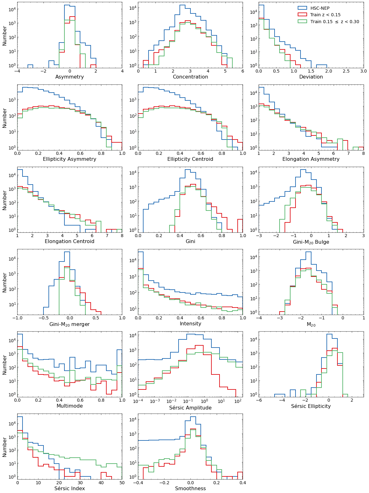
Figure 1: Distributions of morphological parameters for NEP-SCP galaxies (blue), training data for the $z<0.15$ network (red) and training data for the $0.15\leq z<0.30$ network (green). The range shown is that used for training (see Sect. 3.2 and Table 2)

2.3 Known mergers and non-mergers

For supervised learning, it is necessary to have a sample of objects with known labels, here merger or non-merger, to use to train a machine learning algorithm. For this we used the same sample of merging and non-merging galaxies used as a training set in Pearson et al. (2019a). This training sample was selected in Pearson et al. (2019a) using results from the GAMA-KiDS Galaxy Zoo project (Lintott et al. 2008; Driver et al. 2009; de Jong et al. 2013a, b; Holwerda et al. 2019, Kelvin et al. in prep) along with an A-S cut (Conselice 2003) with the A and S parameters used in this selection derived from KiDS $r$-band imaging. These galaxies have a redshift below 0.15. Pearson et al. (2019a) define a merger to be a galaxy with mergers_neither_frac from Galaxy Zoo to be less than 0.5, that is less than half the citizen scientists determined a galaxy had no evidence of tidal tails or evidence of a merger, and had $A>0.35S+0.02$. Non-mergers were defined by Pearson et al. (2019a) to have mergers_neither_frac $>$ 0.5 and $A<0.35S+0.02$.

We limited the sample of galaxies we used to those that lie in both the GAMA-KiDS coverage as well as the HSC-SSP coverage so that all training objects have HSC data available. As such, the sample is smaller than the sample used by Pearson et al. (2019a) as the HSC-SSP DR2 does not cover all of the area covered by GAMA-KiDS. The resulting sample, which is intentionally class balanced, is 1 683 merging galaxies with 1 683 non-merging galaxies. This balance was achieved by randomly removing galaxies from the larger class until there were the same number of merging and non-merging galaxies. The HSC $r$ magnitude distribution for the whole training sample is presented as a function of redshift in Fig. 2. For use while training the networks that will be employed in this work, $r$-band cutouts of 128$\times$128 pixels, corresponding to approximately 21.5$\times$21.5 arcsec, were made. The morphological parameters used within the networks were derived from these cutouts using the statmorph Python package. The square root of the HSC variance maps were used as the weight maps for statmorph. The morphological parameters can be seen in Fig. 1.

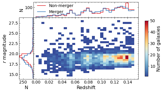
Figure 2: Density plot of HSC-SSP $r$ band magnitude against GAMA spectroscopic redshift for the 3366 training galaxies, both merging and non-merging, binned by $r$ band magnitude and redshift. Blue bins have fewer galaxies and red bins have a larger number of galaxies. Left and upper panels show the $r$ magnitude and redshift distributions, respectively, of the non-merger (red) and merger (blue) galaxies.

As the selection of merging galaxies was aided by the A-S cut, it is likely that the non-merging galaxies have little or no visible structure, a result of the A-S cut splitting featured and non-featured galaxies (Conselice 2003). However, as the merging galaxies are visually selected with Galaxy Zoo, these are likely to be galaxies with the visual appearance of mergers. As a result, the non-mergers selected by a network trained with this data have the potential to be selected due to their lack of features. This provides further justification of visual confirmation of the mergers selected by the neural networks used in this work, beyond the non-merger contamination expected from any machine learning technique.

This work also identified galaxies at redshifts between 0.15 and 0.30. For this, the galaxies used at $z<0.15$ were augmented to appear like higher redshift galaxies. This was done as there is not a sample of known galaxy mergers between these redshifts in GAMA-KiDS or NEP. A random redshift between 0.15 and 0.30 was selected and assigned to each galaxy and the apparent $r$-band magnitude of each galaxy dimmed to match that redshift. For any galaxies whose new apparent magnitude was greater than 26 AB, the approximate $r$-band magnitude limit for the HSC-SSP, 0.15 was added to the original redshift of the galaxy and the apparent magnitude re-calculated. Galaxies whose apparent magnitudes were still above 26 AB were removed. The physical resolutions of the remaining galaxies were adjusted to match their new redshift. Galaxy cutouts that were 256$\times$256 pixels were rebinned to reduce blank space around the resized, 128$\times$128 pixel images that were used for training the networks. Synthetic, Gaussian noise was then added to the image, which also filled any blank space around the resized images. The standard deviation of the synthetic noise was determined by calculating the standard deviation of the original image, before redshift dimming, after 3$\sigma$ clipping 100 times. The clipping derived noise is approximately a factor of 10 larger than the HSC weight maps (that is the maps of the 1$\sigma$ values of each pixel). This larger noise will not be a perfect representation of the real images and so provides further requirement for a visual check to confirm the merger candidates from the neural networks are real mergers. The size of the images was still 128$\times$128 pixels and the synthetic noise was used to fill the empty space around the re-binned image. Segmentation maps were generated using SExtractor and morphological parameters re-derived using statmorph, using the square root of appropriately scaled version of the HSC variance maps as the weight maps, and can be seen in Fig. 1. The scaling of the weight maps includes both the resolution scaling and synthetic noise contribution. The higher noise may also influence the morphological parameters from statmorph. This sample was again class balanced by random removal of galaxies in the larger class.

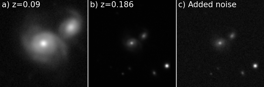
Figure 3: Example of augmentation of a galaxy to a higher redshift. The original galaxy is shown in panel (a), the physically rebinned and dimmed galaxy is shown in panel (b) and the final image, with added Gaussian noise, is shown in panel (c). All panels have asinh scaling and are 128$\times$128 pixels.

K-correction was not applied to these redshifted images. Using the average spectral energy distribution template of Chary & Elbaz (2001), an increase in redshift by 0.15, from $z=0.075$ to $z=0.225$, would require a K-correction of approximately a factor of 1 for the $r$-band (i.e. no correction is required). The same factor is seen using the Wuyts et al. (2008) template while the average SWIRE Template Library template (Polletta et al. 2007) has a factor of $\sim$0.9. The exact K-correction will differ between specific galaxies but this difference is not expected to be large. For the same redshift change, the magnitude is changed by approximately 2.5 or the flux is changed by a factor of approximately 10.

For generating synthetic seeing in the redshifted galaxies, four options were considered. The original image could be deconvolved with the point-spread function (PSF), the image resized and this new image re-convolved with the PSF, which is not possible as deconvolving a noisy image results in the destruction of the image. A second PSF could be calculated to re-create the original PSF in the rescaled images. The resized image could be convolved with the PSF, which would result in over-distortion. Or no alteration could be done, which would result in an under-distorted image. Here we performed no convolution and accept that the resulting images will be under-distorted. The PSF of the original, non-redshifted image was used within statmorph when deriving the morphological parameters. As this is likely to introduce errors in the morphological parameters and cause the images to not be a perfect representation of the real images, this provides further requirement for visual confirmation of the merger candidates from the neural network.

2.4 Mass completeness

For application of the merger sample derived in this work (Sect. 5) it is necessary to determine the mass completeness limit. This mass completeness estimate was done empirically following Pozzetti et al. (2010):

$$log(M_{lim})=log(M_{\star})-0.4(r_{lim}-r),$$ (3)

where M_⋆ is the stellar mass of a galaxy in M_⊙, $r_{lim}$ is the limiting $r$-band magnitude, here set to 26, $r$ is the measured $r$-band magnitude of the galaxy and M_lim is the lowest mass that can be observed for this object at the $r$-band magnitude limit. The limiting mass within a redshift bin is then the M_lim value that 90% of the faintest 20% of galaxies have masses below. The masses of each galaxy were determined at the same time as their photometric redshifts through spectral energy distribution fitting using LePhare (Arnouts et al. 1999; Ilbert et al. 2006; Ho et al. 2021). While this calculation of the completeness limit was for the $I$-band in Pozzetti et al. (2010), we find that using the $r$-band provides a more conservative mass limit. As the galaxy selection, morphologies, and classifications are based on $r$-band data, it was decided to use the more conservative $r$-band mass limit over the $I$-band limit.

3 Deep learning

Deep learning is a subset of machine learning that aims to loosely mimic how biological neural networks process data. This work employs a convolutional neural network (CNN) combined with a traditional neural network. CNNs are designed to better process multi-dimensional data, such as images, by reducing the number of trainable parameters within a network. Here, we specifically perform supervised learning, where the truth values for the training data are known. The training data are typically sub-divided into three subsets: a ‘training set’, which typically contains 70% to 90% of the training data, used to train the network; a ‘validation set’, which typically contains 5% to 15% of the training data, used to evaluate the performance of a network as it is trained; and a ‘test set’, which again typically contains 5% to 15% of the training data, that are not shown to a network during training and only used once to test a network once training is complete. The exact split between the three data sets is a matter of choice and varies between studies: here we use 80% for the training set, 10% for the validation set and 10% for the test set. For ease of communication, neural networks that are not CNNs will be referred to as fully connected networks (FCN).

3.1 Neural network architecture

For this work, we emploied a hybrid neural network containing a FCN and a CNN, the output of which are combined to form a final result (e.g. Zhou & Hauser 2017; Dobbels et al. 2019). The FCN side of the network has morphological parameters passed into it while the CNN has an $r$-band image of the galaxy being classified passed into it. Each part of the network could be used to determine if a galaxy is a merger or non-merger, however we found that the combination of both provides better results (see Sect. 4.2.1). Unless otherwise stated, the hyper-parameters for the layers, activations, batch normalisations, drop out and optimiser were left at the TensorFlow default values.

The FCN side comprises two layers containing 128 neurons. The output layer of this network comprises two neurons, one each for the merger and non-merger probabilities. Rectified linear units (ReLU; Nair & Hinton 2010) are used for activation in the two layers of 128 neurons while softmax activation is used on the output layer when training. Softmax provides output values between zero and one, whose values from each neuron in a layer sum to unity. We note that as the output of the two output neurons sum to unity, it is also possible to achieve the same result with a single output neuron. Also for the layers of 128 neurons, batch normalisation (Ioffe & Szegedy 2015) is applied before ReLU activation, while dropout (Srivastava et al. 2014) is applied after activation in these layers, with a dropout rate of 20%. All layers are fully connected, that is all the neurons in a layer take all the outputs from the layer below as an input. The FCN has 19 328 trainable parameters.

The architecture of the CNN side is based on the CNN of Pearson et al. (2019a, b), itself based on the Dieleman et al. (2015) architecture. The lowest four layers, the four layers to the left of the CNN section of Fig. 4, are convolutional layers while the top two layers, the right most CNN layers in Fig. 4, are fully connected layers. The lowest layer, the left most in Fig 4, comprises 32 6$\times$6 kernels, followed by a layer of 64 5$\times$5 kernels and then two layers with 128 3$\times$3 kernels. All convolutional layers use a stride of 1. As with the FCN, batch normalisation is applied before ReLU activation and 20% dropout is applied after activation for all convolutional layers. After the first, second and fourth convolutional layers, 2$\times$2 max-pooling is performed.

After the convolutional layers, two fully connected layers are used, with 2 048 and 128 neurons. As with the FCN, batch normalisation is applied before ReLU activation and 20% dropout is applied after activation for both fully connected layers. For training this part of the full network, the output layer is again composed of two neurons, one for the merger classification and one for the non-merger classification. As with this FCN, softmax activation is used in this layer with no batch normalisation or dropout. The CNN has 67 652 128 trainable parameters.

The outputs from the last layers of the FCN and CNN are concatenated to form a single layer of 256 values. These are then passed into the Top Network that comprises a fully connected layer of 256 neurons. As with the FCN and fully connected part of the CNN, batch normalisation is applied before ReLU activation. This is followed by 20% dropout while training. The output from the Top Network is a layer with two neurons, one each for the merger and non-merger classes, with softmax activation. The Top Network has 66 818 trainable parameters. The full network can be seen in Fig. 4 and has a total of 67 738 274 trainable parameters.

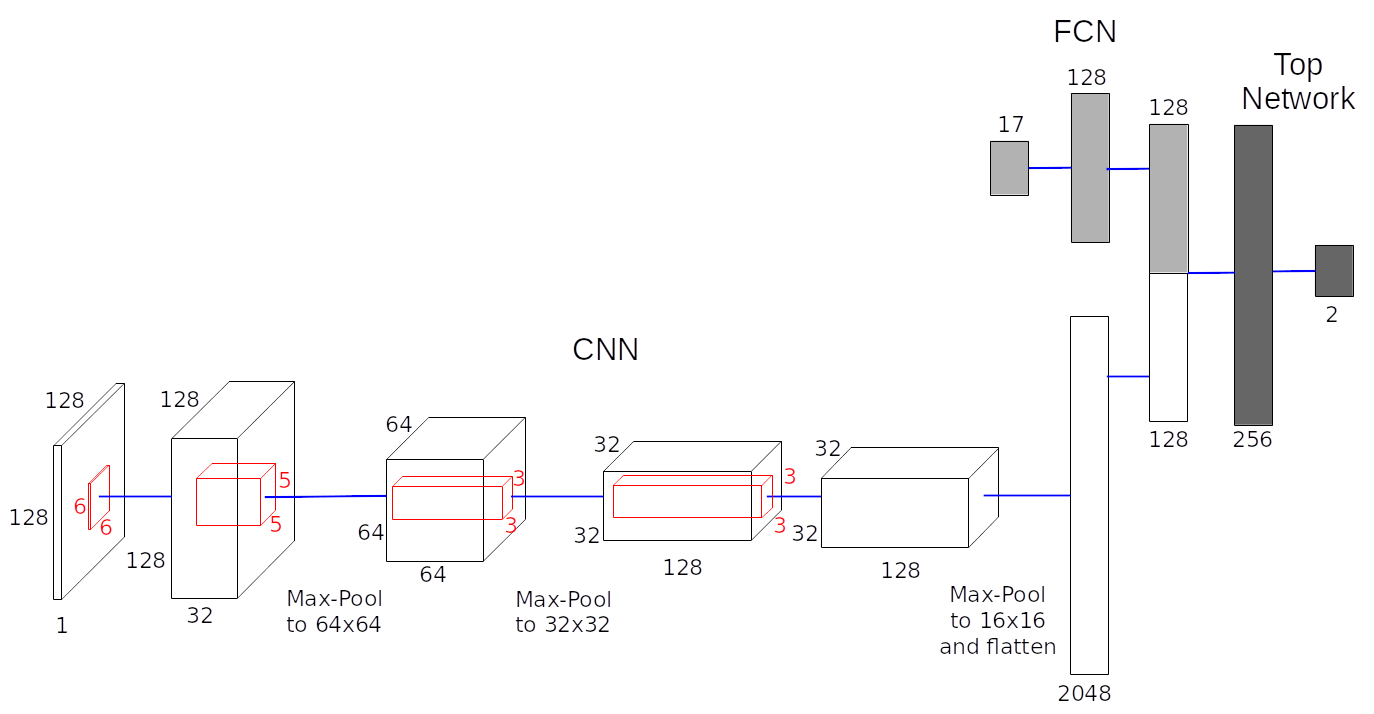
Figure 4: Visual schematic for the full neural network. White regions are the CNN, light shaded regions are the FCN and the dark shaded regions are the Top Network. The input to the CNN is a single band, 128$\times$128 pixel image while the input to the FCN is the 17 morphological parameters. Both of these inputs are on the left of their corresponding part of the network. The output from the full network is on the right as a two neuron, binary classification. The sizes of the kernels for the CNN (red) and fully connected layers for all parts of the network are shown. The blue line between layers represent the batch normalisation, ReLU activation and dropout that is applied between layers. The CNN has 67 652 128 trainable parameters, the FCN has 19 328 trainable parameters and the Top Network has 66 818 trainable parameters. The full network has a total of 67 738 274 trainable parameters.

The CNN, FCN, and Top Network were trained separately (see Sect. 3.2). For each part of the network, the loss of the network was determined using categorical cross-entropy and was optimised using the Adam algorithm (Kingma & Ba 2015). The initial learning rate was $5\times 10^{-5}$ for the FCN, $5\times 10^{-6}$ for the CNN and $5\times 10^{-3}$ for the Top Network. The networks themselves were built using Tensorflow 2.3 (Abadi et al. 2015) and are available on GitHub along with the learnt parameters.

For the FCN, a number of different hyper-parameter values were explored. Three layer and four layer architectures were tested, with no improvement over the used two layer structure. Also, 256 and 1 024 neurons per layer were also tested, again with no improvement over the current architecture. As fewer neurons require less data to effectively train, the smaller size of a two layer network with 128 neurons per layer was chosen.

Few different hyper-parameters were explored for the CNN, as this architecture has been found to perform well in identifying galaxy mergers with data from a number of different surveys (Pearson et al. 2019a, b). However, the number of neurons in the fully connected layers in the CNN were explored, testing 1 024 and 4 096 neurons in the left most fully connected layer in Fig. 4 with no marked improvement to performance.

While testing different architectures for the FCN, the size of the last fully connected layer in the CNN was also changed. As the right most layers of the CNN and FCN (in Fig. 4) are the same size, 256 and 1 024 neurons in this layer were also tested, again showing no change over the architecture used here. The last layers in the FCN and CNN were chosen to be the same size to potentially allow equal weight to be placed on both the morphological parameters and the images. The size of the first layer in the Top Network was matched to the size of the concatenated last layers of the FCN and CNN, and so a layer with 1 024 and 2 058 neurons was also tested, again showing no improvement over the current architecture.

For all three networks, different initial learning rates for the Adam optimiser were also tested. Here, rates of $5\times 10^{-2}$, $5\times 10^{-3}$, $5\times 10^{-4}$, $5\times 10^{-5}$, $5\times 10^{-6}$ and $5\times 10^{-7}$ were tested. The best performing initial learning rate, one for each part of the network, was then chosen.

3.2 Training, validation, and testing

The FCN, CNN, and full network were trained independently. The FCN and CNN were trained first using the galaxy morphologies and images, respectively. The two-neuron output layers were then removed and the trained weights and biases of the FCN and CNN were fixed. The top layers of the FCN and CNN were then concatenated and the results passed into the Top Network, which was then trained. The output of the full network, the FCN, CNN and Top Network, was then the prediction for if a galaxy is a merger or not.

The training data described in Sect. 2.3 were split into three groups. For the $z<0.15$ networks, 2 692 galaxies were used to train the network, 338 were used to validate the network as it trained, and a final 336 were used to test the network. For the $0.15<z<0.30$ network, 2 514 were used to train the network, 314 were used to validate the network and 314 were used to test the network. The same galaxy samples were used to train each part of the network.

To train the FCN, the morphological parameters were scaled between zero and one by subtracting the minimum value in Table 2 and dividing by the range between the minimum and maximum values in Table 2. We note that the values presented in Table 2 do not necessarily directly correspond to the maximum and minimum values of the training data, as seen in Fig. 1. The FCN was trained for 5 000 epochs with the epoch that provided the lowest validation loss being used for training the Top Network and classification. To train the CNN, the images were used. These images were linearly scaled, randomly rotated by 0^∘, 90^∘, 180^∘, or 270^∘, randomly flipped vertically, then randomly flipped horizontally as they were passed into the network. CNN are known to not be rotationally invariant (e.g. Gong et al. 2014; Mopuri & Babu 2015; Chandrasekhar et al. 2016), while the morphology of a galaxy is independent of rotations in the plane of the sky. Thus this rotation and flipping will help generalisability of the network (e.g. Dieleman et al. 2015; Huertas-Company et al. 2018). Redshifts of the galaxies were not used inside the networks as the networks would need to be designed with a specific number of redshifts to be passed into it. As the number of galaxies (background and foreground) within each image will be different, some images will have more galaxies than a specified number and others fewer, it was decided to not include these data. The CNN was trained for 200 epochs with the epoch that provided the lowest validation loss being used for training the Top Network and classification. The Top Network was trained for 1 000 epochs with the epoch that provided the lowest validation loss being used for classification.

Table 2: Minimum and maximum values used to scale the morphological parameters

Parameter	Minimum	Maximum
Asymmetry (A)	-4.0	4.0
Concentration (C)	0.0	6.0
Deviation (D)	0.0	3.0
Ellipticity asymmetry (Eli A)	0.0	1.0
Ellipticity centroid (Eli Cen)	0.0	1.0
Elongation asymmetry (Elo A)	1.0	8.0
Elongation centroid (Elo Cen)	1.0	8.0
Gini	0.0	1.0
Gini-M20 bulge (GMB)	-3.0	3.0
Gini-M20 merger (GMM)	-1.0	1.0
Intensity (I)	0.0	1.0
M20	-4.0	0.0
Multimode (M)	0.0	1.0
Sérsic amplitude (SA)	0.0	200.0
Sérsic ellipticity (SE)	-6.0	3.0
Sérsic index ($n$)	0.0	50.0
Smoothness (S)	-0.4	0.4

4 Results

4.1 Morphological Parameters

Here we examine the morphological parameters that were used to train the neural networks. As can be seen in Fig. 1, some of the derived asymmetries are negative; due to the asymmetry being a sum of residuals, it should always be positive. In theory, the intrinsic asymmetry of a galaxy should be positive but it cannot be measured directly due to the presence of noise. As an attempt to remove the contribution of the background, the corrected asymmetry A_corr = A_obs - A_bkg is typically used (Conselice et al. 2000), where A_obs is the uncorrected asymmetry and A_bkg is the asymmetry of the background. Therefore, negative asymmetries are mathematically allowed as a result of over-correcting for the asymmetry of the background. In general, correctly accounting for noise when measuring the asymmetry parameter is a non-trivial task and is still the topic of active research (e.g. Thorp et al. 2021). Large fractions of negative asymmetry, and smoothness as also seen here, are also found in other observational works (e.g. Rodriguez-Gomez et al. 2019; Sazonova et al. 2020). Inspection of the positioning of the skyboxes, used to estimate the background noise, and the segmentation maps for a random sample of objects with negative asymmetry did not greatly differ from a random sample of galaxies with positive asymmetry. Thus, we deem the asymmetry and smoothness to be adequate for this work.

We also note that there are negative Sérsic ellipticities in Fig. 1 as well as values above unity. While the Sérsic ellipticity should lie between zero and unity, statmorph allows for fitting to values outside of this range. These can be converted to an equivalent ellipticity (SE^′) within the range [0,1] using SE^′ = min(SE, 2-SE) for SE $>1$ or SE^′ = max(SE, SE/(SE-1)) for SE $<0$. As these conversions are simple we elected to use the Sérsic ellipticity from statmorph in this work without conversion. Use of the Sérsic ellipticity in the presented with this paper in future works should use these conversions.

To check the validity of the morphologies used to train the networks, the morphological parameters of the $z<0.15$ training data derived from the HSC-SSP images were compared to those derived from GAMA-KiDS data in Pearson et al. (2019a). This allows the comparison of the morphologies of the same galaxies using different data. The morphological parameters from the HSC-SSP data were subtracted from those of the GAMA-KiDS data, with the resulting differences ($\delta$) presented in Table 3. Outliers are defined as galaxies whose morphological parameters are outside of 5$\sigma$ of the mean, where $\sigma$ is the sample standard deviation.

Table 3: Comparison between morphological parameters derived from HSC-SSP images used to train the low redshift network in this work and derived from GAMA-KiDS data in Pearson et al. (2019b). These differences are expressed the value from HSC-SSP morphological parameters subtracted from the GAMA-KiDS morphologies ($\delta$): negative means imply that HSC-SSP morphologies are larger than GAMA-KiDS.

Parameter	Mean $\delta$	Std $\delta$	Outliers
Asymmetry (A)	-0.060	0.087	22
Concentration (C)	-0.052	0.299	26
Deviation (D)	0.011	0.097	28
Ellipticity asymmetry (Eli A)	-0.003	0.095	22
Ellipticity centroid (Eli Cen)	-0.003	0.096	22
Elongation asymmetry (Elo A)	0.073	2.882	4
Elongation centroid (Elo Cen)	0.051	2.694	2
Gini	0.010	0.052	21
Gini-M20 bulge (GMB)	0.027	0.235	14
Gini-M20 merger (GMM)	0.013	0.068	24
Intensity (I)	-0.023	0.160	38
M20	0.029	0.200	28
Multimode (M)	0.000	0.158	55
Sérsic amplitude (SA)	0.330	1.077	21
Sérsic ellipticity (SE)	-0.044	0.150	33
Sérsic index ($n$)	-0.433	6.744	9
Smoothness (S)	-0.039	0.367	24

Generally, the results using the HSC-SSP are in good agreement with the morphologies from GAMA-KiDS. For the Sérsic amplitude, as the photometric zero-points and pixel areas are different for HSC-SSP and KiDS, the comparison is made with the surface brightness in mag arcsec^-2 and not the counts, the latter of which are presented in Table 1 and Pearson et al. (2019a). Thus, the positive mean $\delta$ for SA indicates that the HSC-SSP values are brighter than the GAMA-KiDS values.

None of the resulting distributions are Gaussian, thus we cannot use the expected number of 5$\sigma$ outliers to check the closeness of fit. Chebyshev’s inequality restricts the number of objects more than 5$\sigma$ from the mean to be 1/25 of the total number of objects, that is no more than 134 of the 3 366 galaxies can be classified as outliers. For all but Multimode and Intensity, there are fewer outliers than a quarter of this value. Multimode and Intensity also have the most non-Gaussian distributions so the higher numbers of outliers may be expected.

Elongation asymmetry, elongation centroid, and Sérsic index have large standard deviations. For the elongation asymmetry and centroid, these large standard deviations are driven by large values from the GAMA-KiDS morphologies; all outliers have large parameter values compared to the rest of the population. For the Sérsic index, the large standard deviation is driven by a small number of galaxies with a large Sérsic index in either the HSC-SSP data or GAMA-KiDS, with four out of nine of the outliers being due to large $n$ in GAMA-KiDS and five being due to large HSC-SSP $n$.

4.2 Galaxy mergers

In this section, we present the results of our model’s test performance and outline our visual inspection programme. An example of the final catalogue is presented in Table 4. The results from the neural networks are given as the probability that a galaxy is a merger or non-merger, frac_merger and frac_nonmerger respectively. It also has the classification from visual inspection as vis_merger (see Sect. 4.2.2 below). Randomly selected examples of HSC-NEP galaxies identified as non-mergers by the networks, as mergers by the networks but not visual inspection, and as mergers by visual inspection are presented in Fig. 5. Here, we take galaxies with frac_merger $>0.5$ to be identified as mergers by the networks (hereafter merger candidates).

Table 4: Ten rows of the catalogue of merging galaxies in NEP

HSC_ID	RA	Dec	frac_merger	frac_nonmerger	vis_merger
79217643822780147	270.743	65.328	0.572	0.428	False
79217643822780325	270.782	65.341	0.988	0.012	False
79217643822780333	270.789	65.343	0.025	0.975	False
79217643822780337	270.795	65.340	0.056	0.944	False
79217643822781103	270.745	65.346	0.088	0.912	False
79217648117743947	270.775	65.386	0.182	0.818	False
79217648117753062	270.734	65.374	0.056	0.944	False
79217648117753093	270.758	65.361	0.145	0.855	False
79217648117753463	270.737	65.374	0.286	0.714	False
79666772847897740	267.434	65.748	0.959	0.041	True
…	…	…	…	…	…

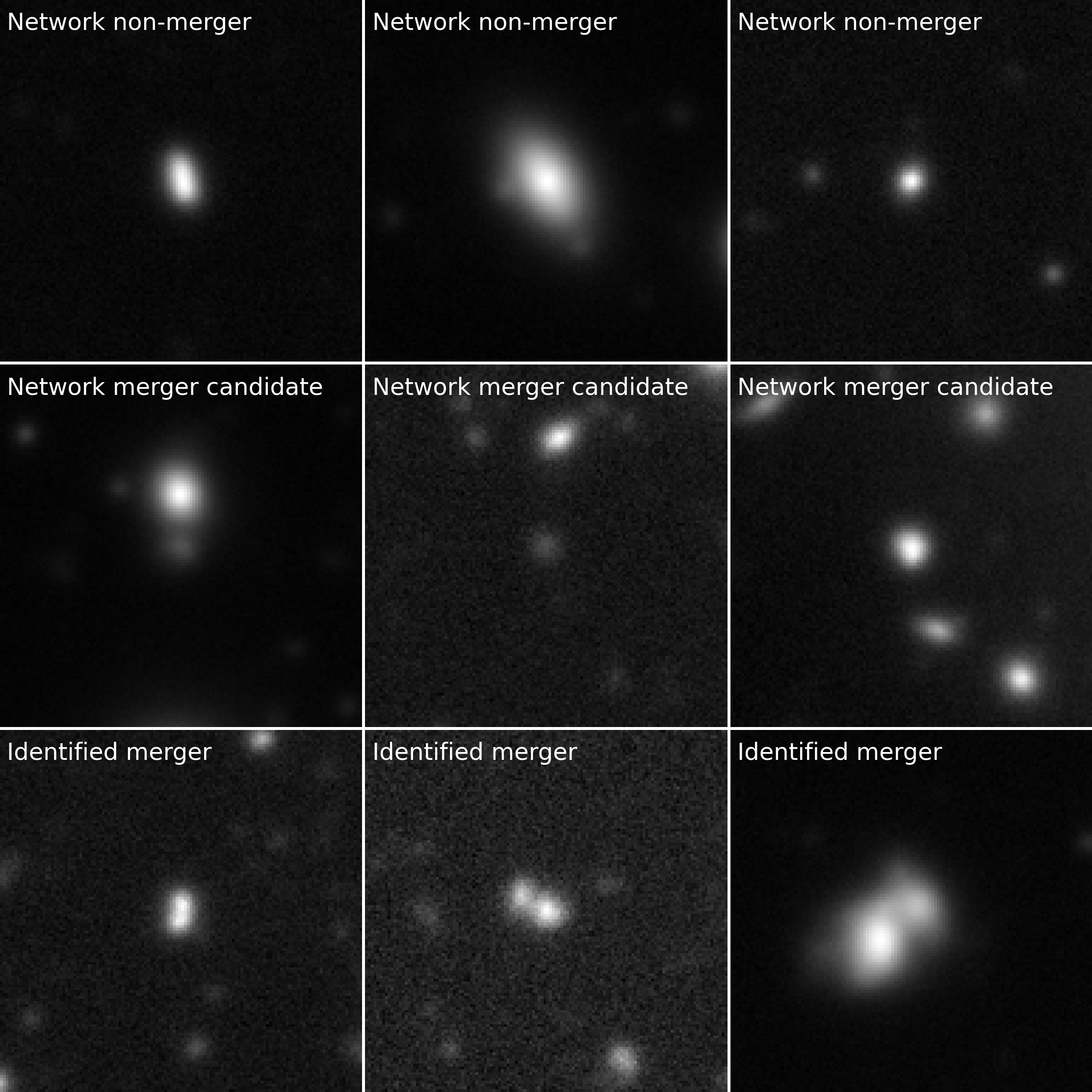
Figure 5: Randomly selected HSC-NEP galaxies as example for galaxies selected by the networks as non-mergers (top row), galaxies selected as merger candidates by the networks but not identified as mergers by visual inspection (middle row), and galaxies selected as galaxy mergers by visual inspection (bottom row). The classified galaxy lies in the centre of the 128$\times$128 pixel ($\approx$ 21.5$\times$21.5 arcsec) image and the images are shown with asinh scaling.

4.2.1 Neural networks

In determining the architecture of the neural network, it was found that combining a FCN and CNN had better performance than a FCN or CNN alone. Tests with the $z<0.15$ data set, the validation of the best FCN had a loss of 0.301 and accuracy of 88.8% while the validation of the best CNN had a loss of 0.473 and accuracy of 79.3%. When combining the FCN and CNN, as described in Sect. 3.1, the validation of the final full network for $z<0.15$ galaxies has a loss of 0.260 and accuracy of 91.7%. It would be expected that there is information contained in the images that is not present in the morphological parameters: the morphological parameters can be seen as a compression of the information of the images. However, this result suggests that there is information in the morphological parameters that is not present in the images, or more likely the information in the morphological parameters is more easily extracted by a neural network than the information in the images. This difficulty may lie in the noise or background of the image confusing the network. The same noise or background may present a similar issue for the morphological parameter extraction but the network itself is presented the pre-extracted parameters. Thus, combining the images and morphologies allows the network to supplement the more easily interpreted morphological parameters with further, harder to extract information contained within the images. As a result, it is not entirely surprising that the network performs better combining the images with the morphological parameters than either alone despite both containing similar information.

The quality of the two full networks, one for $z<0.15$ and one for $0.15\leq z<0.30$, can be determined by the results presented in Table 5. Due to the training set being class balanced while mergers are expected to be in the minority of real galaxies, we caution the use of accuracy alone to determine the quality of a network when applied to non-class balanced data.

The trained networks described in Sects. 3.1 and 3.2 were applied to galaxies in the North Ecliptic Pole. Taking a galaxy with frac_merger greater than 0.5 as a merger candidate, these classifications resulted in 1 477 of 6 965 galaxies at $z<0.15$ and 8 718 of 27 299 galaxies at $0.15\leq z<0.30$ being identified as galaxy merger candidates. This results in a merger candidate fraction of 21.2% for the lower redshift range and 31.9% for the higher redshift range.

Table 5: Performance statistics from the neural networks. All values calculated with the class balanced test data set.

Redshift	Statistic	Value
$z<0.15$	Accuracy	0.884
	Recall	0.863
	Precision	0.901
	Specificity	0.905
	NPV	0.869
$0.15\leq z<0.30$	Accuracy	0.850
	Recall	0.790
	Precision	0.899
	Specificity	0.911
	NPV	0.812

4.2.2 Visual Inspection

As we expect there to be a large number of falsely identified galaxy mergers in the merger candidates identified by our full networks, the galaxies identified as galaxy merger candidates by the full network were visually checked by two authors, the majority by WJP and a minority by LES. Discussion of the quality of the visual classifiers can be found in Appendix B. The visual classification includes considering the redshifts of galaxies close to the merger candidate to check for close companions. If both WJP and LES inspected a merger candidate, a galaxy was only considered a merger if both WJP and LES considered the galaxy to be a merger. This resulted in 251 of 1 477 being true mergers at $z<0.15$ and 1858 of 8718 being true mergers at $0.15\leq z<0.30$. This results in a merger fraction of $3.6\%$ for $z<0.15$ and $6.8\%$ for $0.15\leq z<0.30$. However, due to the difficulties in visual classification, it is possible that some of the galaxies identified as merger candidates by the networks could truly be mergers but misclassified as non-mergers during visual inspection.

With the large number of non-merging galaxies that would need to be visually checked, it was deemed too time costly to visually confirm all non-mergers. As the number of mergers is expected to be low and the recall of the network is high, very few true mergers (approximately 13.7% at $z<0.15$ and 21.0% at $0.15\leq z<0.30$) are expected to be classified as non-mergers and so few mergers are expected to be missed. Using the recall of the two full networks presented in Table 5 and the number of visually confirmed mergers, we expect to miss approximately 40 mergers at $z<0.15$ and approximately 494 at $0.15\leq z<0.30$.

However, as discussed in Appendix B, the visual classifications are not complete with a recall of 0.45. If we combine this with the network performances presented in Table 5, we expect the final visually selected merger samples to be 38.8% complete at $z<0.15$ and 35.6% complete at $0.15\leq z<0.30$. The test merger candidate samples contain 9.5% and 8.9% of all non-mergers at $z<0.15$ and $0.15\leq z<0.30$, respectively. Again combining these with the average specificity of the visual classifiers, the visually selected merger samples contain 1.9% and 1.8% of all non-mergers at $z<0.15$ and $0.15\leq z<0.30$, respectively. If we take the true merger fractions to be 3.6% at $z<0.15$ and 6.8% at $0.15\leq z<0.30$, this implies the visually confirmed merger samples are 43.3% pure at $z<0.15$ and 59.0% pure at $0.15\leq z<0.30$. However, as the visual classification was done on a pre-selected sample of merger candidates while the discussion in Appendix B was performed with a class balanced sample of mergers and non-mergers with no pre-selection on morphologies, the quality of the visual classifiers may be lower than presented, a result of a pre-selected sample likely being harder to differentiate between mergers and non-mergers than an unselected sample.

We also visually inspected a small sample of galaxies identified as non-mergers, 100 from the $z<0.15$ network and 100 from the $0.15\leq z<0.30$ network. Within both of these samples we found no obvious misclassifications, supporting the expectation that very few mergers were misclassified as non-mergers by the networks. A summary of the number of galaxies identified as non-merger, merger candidates and visually selected mergers is presented in Table 6.

Table 6: Summary of the number of galaxies identified as non-mergers, merger candidates and visually confirmed mergers

	Total galaxies		Merger candidate	Confirmed merger
Redshift		Non-merger
$z<0.15$	6 965	5 488	1 477	251
$0.15\leq z<0.30$	27 299	18 581	8 718	1 858

During visual inspection, the non-mergers were also briefly checked for true non-merging galaxies with visible structure. This is due to the training sample possibly causing the networks to be trained on structureless and structured galaxies, and not mergers and non-mergers, as discussed in Sect. 2.3. The brief visual inspection found that there were galaxies identified as non-mergers that did contain resolvable structure, such as spiral arms, as can be seen in Fig. 6. Similarly, there are merger candidate galaxies that have no visible structure, as shown in Appendix C. Thus, the networks have not been inadvertently trained to find structured and non-structured galaxies.

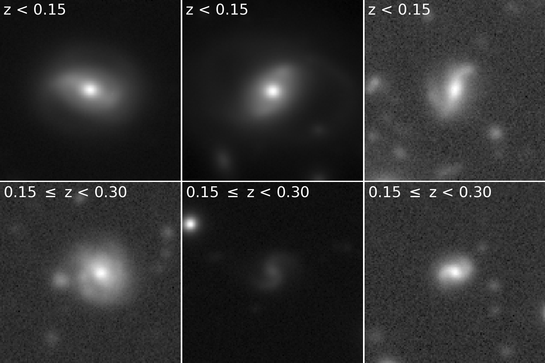
Figure 6: Examples of visually confirmed non-mergers with visible structure. The top row shows non-mergers detected by the $z<0.15$ network and the bottom row shows non-mergers detected by the $0.15\leq z<0.30$ network.

5 Discussion

5.1 False positives

While it is expected that there will be false positive (FP) detections from the networks, that is galaxies that are identified by the full network as a merger which are non-mergers, it is informative to understand why such galaxies are misclassified.

5.1.1 Image Occlusion

To understand which visual properties of the FP galaxies were being identified for galaxies at $z<0.15$, occlusion experiments (e.g. Zeiler & Fergus 2014; Ancona et al. 2018; Pearson et al. 2019b; Wang et al. 2020) were performed on four FP galaxies with frac_merger$\approx$0.76 (galaxies b, d, j, and l in Fig. 7) and four with frac_merger$\approx$0.99 (galaxies f, h, n, and p in Fig. 7). Eight true positive (TP) galaxies were also selected for occlusion experiments: four with frac_merger$\approx$0.76 (galaxies a, c, i, and k) and four with frac_merger$\approx$0.99 (galaxies e, g, m, and o). For this experiment, a $16\times 16$ pixel region of the images were set to zero. The $16\times 16$ pixel zero region was translated across the image by one pixel such that there were a total of 12 769 copies of the galaxy with a different $16\times 16$ pixel regions set to zero. These occluded images were then passed through the full network with the morphological parameters left unchanged. The occluded galaxy images are treated as a normal galaxy by the networks and so are scaled by the networks to be between zero, the faintest pixel in the occluded image, and one, the brightest pixel in the occluded image. Heat maps were then generated by taking the average classification for when each pixel was occluded. Figure 7 shows these heat-maps along with the original image of the galaxy.

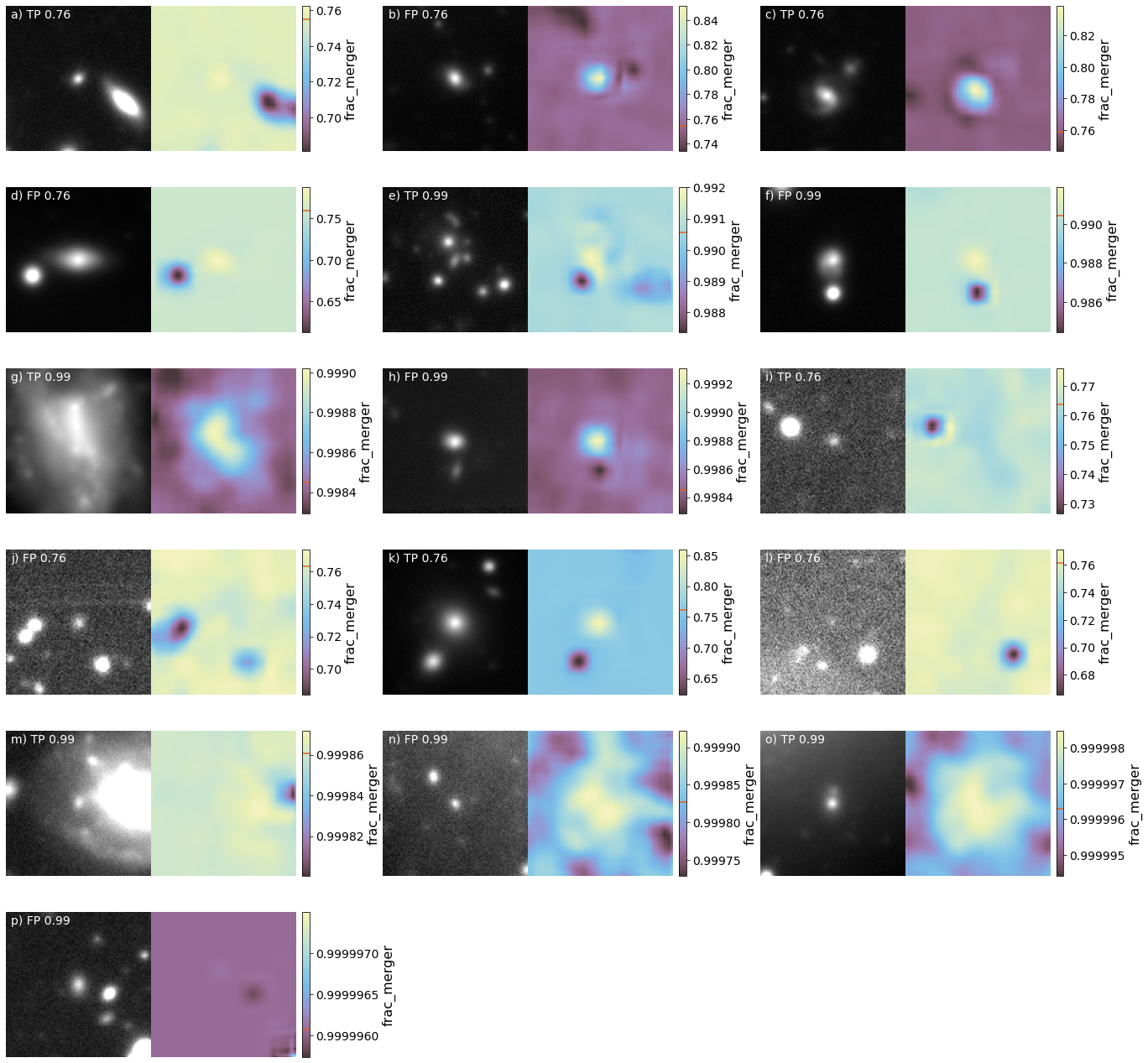
Figure 7: Galaxy images and associated feature importance heatmaps for sixteen galaxies at $z<0.15$. The sixteen galaxies comprise of four TP galaxies with frac_merger$\approx$0.76, four TP galaxies with frac_merger$\approx$0.99, four FP galaxies with frac_merger$\approx$0.76, and four FP galaxies with frac_merger$\approx$0.99, as indicated in the upper left corners of the galaxy images. The panels to the right of the galaxy images contain the heat maps for feature importance, with pixels that when obscured cause the galaxy to have lower frac_merger in dark purple and pixels that cause the galaxy to have a higher frac_merger in light yellow. The orange line in the colour bar indicates the frac_merger of the un-occluded galaxy.

The heat-maps in Figs. 7a and 8 indicate the regions that are important for the CNN part of the network to identify a merging galaxy. Each pixel within these images indicates the average change of classification when the pixel is occluded. As the average is of up to 256 values, large changes when the pixel is occluded will be suppressed. This means that Figs. 7 and 8 are primarily useful for qualitative analysis. Thus, while no galaxies seen in these figures show a change in classification and suggest the classification is primarily driven by the morphologies, these plots cannot be used for such definitive statements.

For all FPs, the presence of the second galaxy in the frame is an important component used for classification. These secondary galaxies are not physically associated with the primary galaxies in the centre of the image due to their different redshifts. Occlusion of these secondary galaxies reveals that the full network is interpreting them as potential merging companions.As the redshift information is not passed into the network, this is a somewhat understandable mistake. However, the weak reliance on the images by the full network means the presence of the secondary galaxy in the image is not of great importance overall.

The secondary galaxy influencing classification is also seen with the TPs (a), (e), (i), (k), and (m). For the remaining TPs, instead of being influenced by a secondary galaxy the network is identifying faint features around the primary galaxy, likely signatures of tidal disruption.

From the comparison of the FP and TP, there is the suggestion that including the redshift of the primary and secondary galaxies may aid in determining if two galaxies are indeed merging or are just close in projection but are not physically associated. This was not done due to the reasons previously outlined in Sect. 3.2.

The majority of galaxies show that the primary galaxy is also used in determining the classification. Only galaxies (i), (j), (l), (m), and (p) do not show this behaviour. It is unclear why obscuring the primary galaxy makes a galaxy more likely to be seen to contain a merger. Hiding of the central source may make fainter structures around the galaxy more apparent and hence easier to identify as a merger, but this is speculation.

For the higher redshift network, the image occlusion provides similar results, as seen in Fig. 8. All FP galaxies show the presence of a secondary galaxy is important for classification, with an apparent reduction infrac_merger when it is abscured. Only the TP (i) and (m) galaxies do not see a reduction when a secondary galaxy is obscured. In the case of (i), the merging galaxies are very close to one another making obscuration of a single galaxy of the pair difficult. The high redshift network also sees an influence to classification when the primary galaxy is obscured for galaxies (a), (d), (g), (h), (j), (l), (m), (n), and (p), similar to the low redshift network.

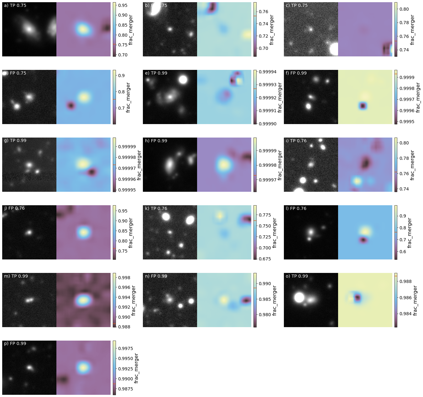
Figure 8: Same as Fig. 7 but for the $0.15\leq z<0.30$ network. Galaxy images and associated feature importance heatmaps for sixteen galaxies at $0.15\leq z<0.30$. The sixteen galaxies comprise of four TP galaxies with frac_merger$\approx$0.76, four TP galaxies with frac_merger$\approx$0.99, four FP galaxies with frac_merger$\approx$0.76, and four FP galaxies with frac_merger$\approx$0.99, as indicated in the upper left corners of the galaxy images. The panels to the right of the galaxy images contain the heat maps for feature importance, with pixels that when obscured cause the galaxy to have lower frac_merger in dark purple and pixels that cause the galaxy to have a higher frac_merger in light yellow. The orange line in the colour bar indicates the frac_merger of the un-occluded galaxy.

However, none of the sixteen, higher redshift galaxies that had the occlusion experiment performed show the importance of faint structures. This does not mean that such structures are not important to the network, just that such structures are not important for the sixteen galaxies shown. Galaxy (i) also exhibits occlusion behaviour that is opposite to what is seen in all other galaxies at both redshifts. For galaxy (i), the occlusion of the primary galaxy reduces frac_merger while the occlusion of the bright object in the field of view increases frac_merger.

We also fully occluded all galaxies, that is we passed an array of zeros in place of the image into the network, and compared the resulting frac_merger with the original classification. As can be seen in Fig. 9a, the low redshift network’s new classifications are typically slightly higher for the fully occluded images at lower frac_merger before becoming consistent at higher frac_merger. There is a positive correlation between the two classifications, although with a large scatter of approximately 0.1. This suggests that, while useful in determining classification, the images are not a strong influence on the classification when compared to the morphologies being fully occluded (Sect. 5.1.2).

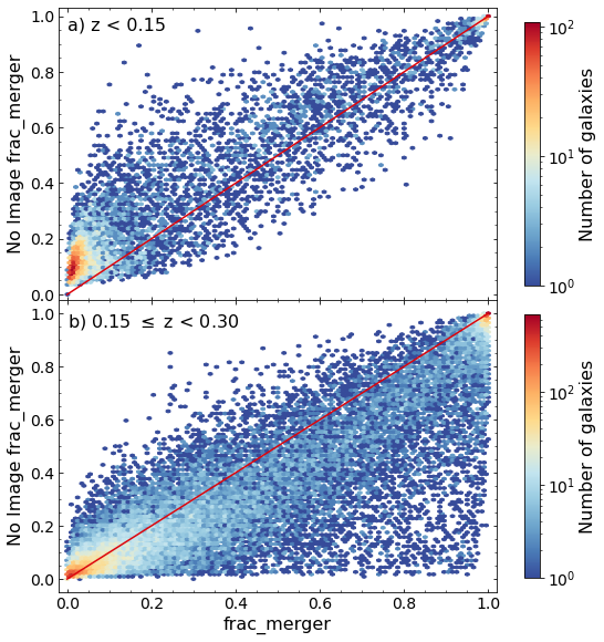
Figure 9: frac_merger when the image is occluded as a function of the original frac_merger for all galaxies classified by the low redshift network (panel a) and the high redshift network (panel b). Number density of galaxies is shown from low (dark blue) to high (red). The 1-to-1 line is shown in red.

For the high redshift network, there is good agreement between the original frac_merger and the image occluded frac_merger at low frac_merger. As frac_merger increases, the occluded frac_merger typically has a lower value, as can be seen in Fig. 9b. There is a large number of objects with the occluded frac_merger close to zero while the un-occluded frac_merger is much larger, a trend not seen in the lower network. This suggests that the images have more importance for the classification than the lower redshift network. However, the correlation between the original frac_merger and the occluded frac_merger suggests that the images still play a minor roll in classification. The morphological parameter occlusion discussed below is in support of the minor importance of the images for the higher redshift network.

5.1.2 Morphological Parameter Occlusion

Occlusion experiments similar to those applied to the images are difficult to perform with the morphological parameters. The lowest input morphological value into the full network is zero by design (see Sect. 3.2) and passing negative values could result in unpredictable and non-interpretable behaviour. Instead of setting each morphological parameter to zero, we instead change the value of each parameter. The range of each parameter in Table 2 was split into 802 equally spaced steps. For each of the 32 galaxies in Figs. 7 and 8, each morphological parameter was set to each of these 802 values one at a time. For example, the asymmetry was set to -4 while all other parameters and the image were left alone. As GMB and GMM are linear combinations of Gini and M₂₀, we also alter Gini or M₂₀ as described above and perform the corresponding change to GMB and GMM following Eqns. 1 and 2, respectively. These are presented in Figs. 10 and 11 as ‘Gini (with GMB, GMM)’ and ‘M₂₀ (with GMB, GMM)’. While altering Gini, M₂₀, GMB or GMM individually is not representative of real world applications, we make these comparisons for completeness. These galaxies with modified morphological parameters were then classified by the full network so the change in classification as each parameter is changed can be studied. The resulting changes in frac_merger as the morphological parameters are changed are shown in Fig. 10 for the $z<0.15$ network and Fig. 11 for the $0.15\leq z<0.30$ network.

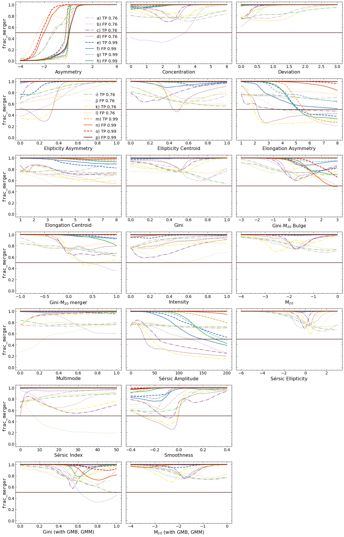
Figure 10: Change in frac_merger due to change in the morphological parameters for sixteen galaxies at $z<0.15$: four TP galaxies with frac_merger$\approx$0.76 (dot-dashed lines), four TP galaxies with frac_merger$\approx$0.99 (dashed lines), four FP galaxies with frac_merger$\approx$0.76 (dotted lines), and four FP galaxies with frac_merger$\approx$0.99 (solid lines). The horizontal line indicates the decision threshold with the merger class being above and the non-merger class being below the line. The sixteen galaxies correspond to the sixteen galaxies in Fig. 7.

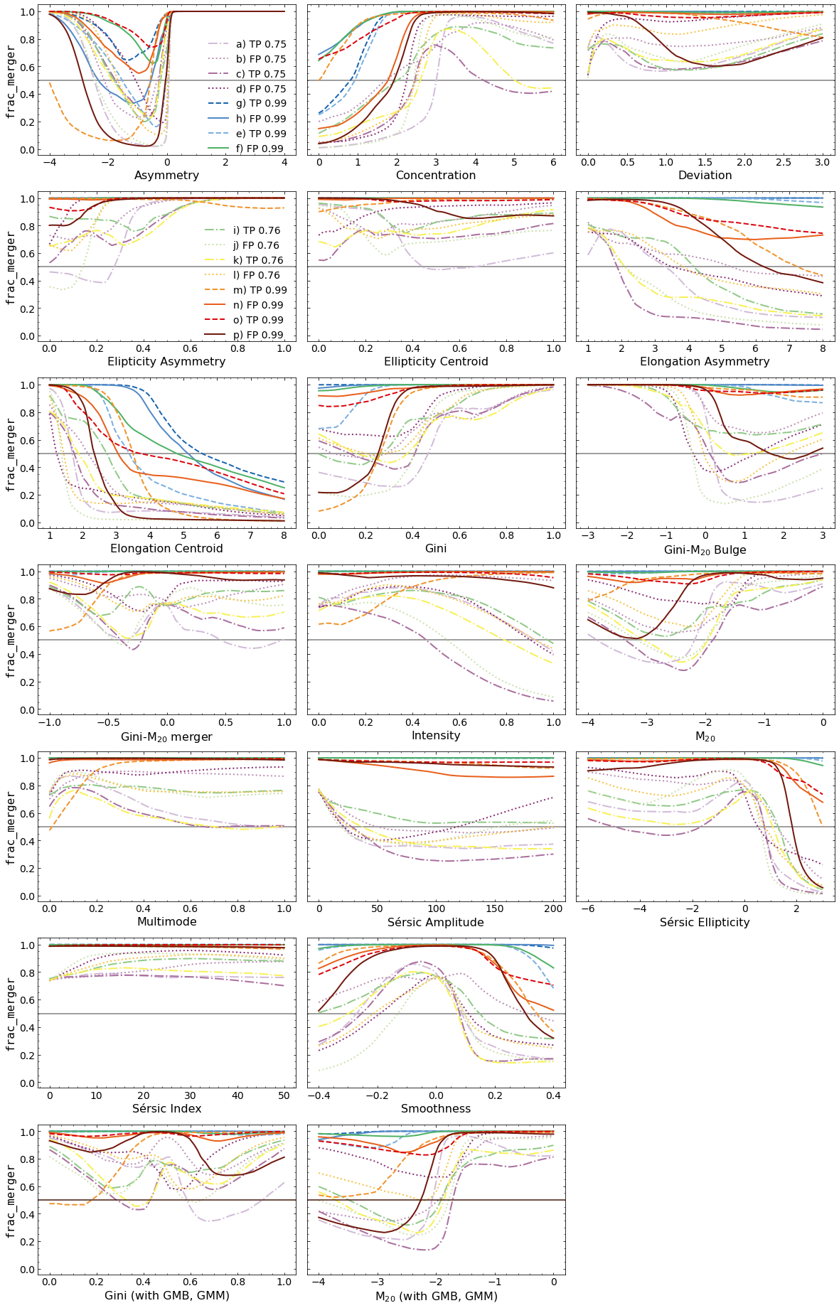
Figure 11: Same as Fig. 10 but for the $0.15\leq z<0.30$ network. Change in frac_merger due to change in the morphological parameters for sixteen galaxies: four TP galaxies with frac_merger$\approx$0.76 (dot-dashed lines), four TP galaxies with frac_merger$\approx$0.99 (dashed lines), four FP galaxies with frac_merger$\approx$0.76 (dotted lines), and four FP galaxies with frac_merger$\approx$0.99 (solid lines). The horizontal line indicates the decision threshold with the merger class being above and the non-merger class being below the line. The sixteen galaxies correspond to the sixteen galaxies in Fig. 8.

Changing the morphological parameters alters frac_merger in all cases. However, changes in D, Gini, M₂₀, I, SE and M₂₀ (with GMB, GMM) do not result in a change of classification for any of the 16 $z<0.15$ galaxies studied. Thus, these parameters are the least important in this network for determining the classification of the galaxy. For a further five parameters, C, Eli Cen, Elo Cen, M, and $n$, only one of the sixteen galaxies sees a change in classification, again indicating that these parameters play a minor role in classification for the $z<0.15$ network. For these parameters, the galaxies that see a change in classification are all FP with frac_merger$\approx$0.76.

While Gini and M₂₀ are often used to identify galaxy mergers (e.g. Lotz et al. 2004, 2008), as the training sample was not selected using these parameters it is perhaps not surprising that these two parameters have little importnace. This is also not due to the presence of linear combinations of Gini and M₂₀ in GMB and GMM. When GMB and GMM are changed along with Gini or M₂₀ as per their definitions, changing M₂₀ (with GMB, GMM) does not result in a change in classification for any of the sixteen galaxies while changing Gini (with GMB, GMM) only sees a change in classification for two of the galaxies.

In the other extreme, only changing A changed the classification of all sixteen galaxies at $z<0.15$, indicating that this is a powerful morphological parameter for identifying merging systems. The Elo A also sees changes in classifications for half of the galaxies studied in detail, further indicating the importance of an asymmetric light distribution in identifying merging galaxies. The Eli A, however, sees changes for fewer galaxies: only three of the sixteen galaxies see a change to classification.

For the remaining parameters for the $z<0.15$ galaxies, the SA sees a change in classification for half of the sixteen galaxies, indicating that it is an important parameter for this network. The S parameter sees a change in the classification for two TP frac_merger$\approx$0.76 galaxies and one FP frac_merger$\approx$0.76 galaxy. The GMB shows a change in classification for one FP frac_merger$\approx$0.76 galaxy and one FP frac_merger$\approx$0.99 galaxy, while GMM sees a change in classification for two galaxies. We reiterate that changing GMB or GMM independently of Gini or M₂₀ is not representative of the real world and so limited understanding can be gained from changing these two parameters in isolation.

For the higher redshift network, only changes in D and $n$ do not result in a classification change for all sixteen galaxies. In the other extreme, only changing the Elo Cen changes the classification for the $0.15\leq z<0.30$ galaxies studied. Like the $z<0.15$ network, asymmetry is again important for classification for the $0.15\leq z<0.30$ network, with only two FP frac_merger$\approx$0.99 and two TP frac_merger$\approx$0.99 galaxies not showing a change in classification. Elo A is again shows a change in classification, here for ten of the galaxies. The galaxies that do not see change to the classification all have frac_merger$\approx$0.99. This again highlights the importance of an asymmetric light distribution in identifying merging galaxies.

Concentration is more important for the higher redshift network than the lower redshift network, with only two FP frac_merger$\approx$0.99 and two TP frac_merger$\approx$0.99 galaxies seeing no change in classification. Gini and M₂₀ are also more important in the higher redshift network than the lower redshift network, with Gini causing a change in classification to nine galaxies and M₂₀ causing a change to four galaxies. GMM and GMB also cause changes to classifications in more galaxies in the higher redshift network than the lower redshift network. Again, changing these four parameters in isolation is not realistic. Changing Gini and M₂₀ with GMB and GMM also shows a greater influence on the classification than the lower redshift network. Gini (with GMB, GMM) sees a change in classification for five of the sixteen galaxies while M₂₀ (with GMB, GMM) sees a change for seven of the galaxies. This again indicates the stronger reliance on Gini and M₂₀ for the higher redsift network compared to the lower redshift network.

The changes in frac_merger for the morphological parameters were much larger than seen in the occlusion experiments. This supports the idea that the morphological parameters are more important to the full networks than the images for both the $z<0.15$ and $0.15\leq z<0.30$ networks. Generally, the higher redshift network appears to rely on a number of different parameters for the classification of galaxies while the lower redshift network primarily sees changes for the parameters that measure the asymmetry of the light distribution. We note caution, however, as these examinations have only been conducted with a small number of galaxies.

As with the images, we have also occluded the morphologies for all galaxies by setting each morphological parameter to the minimum value in Table 2 in place of the correct parameter value. For the low redshift network, this sets the frac_merger for all galaxies close to unity, as can be seen in Fig. 12a. As the image occlusion resulted in a changed but correlated new frac_merger value, it is apparent that the morphology is the main component used for classification of the galaxies as occluding the morphology has a much larger impact on the resulting frac_merger. If the images provided no information for classification, then all the galaxies would all have the same frac_merger when the morphologies are occluded.

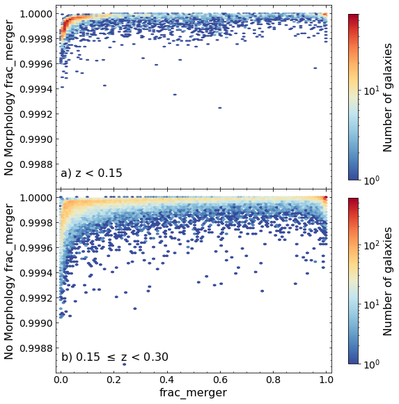
Figure 12: frac_merger when all morphological parameters are occluded as a function of the original frac_merger for all galaxies classified by the low redshift network (panel a) and the high redshift network (panel b). Number density of galaxies is shown from low (dark blue) to high (red).

A similar trend is seen with the high redshift network. When the morphological parameters are to the minimum value in Table 2, the frac_merger of all galaxies becomes close to unity, as can be seen in Fig 12b. Again, the large change in frac_merger when the morphologies are occluded while the changes to frac_merger due to image occlusion are not as severe implies that the high redshift network is primarily using information from the morphologies to determine the classification.

5.2 Merger fraction

As a simple application of the catalogue, it is possible to examine how the merger fraction changes as a function of redshift using the visually confirmed mergers. Here we used redshift bins with width 0.025 and determine the mass completeness within each redshift bin as outlined in Sect. 2.4 and shown in Fig. 13. Once the sample of galaxies within each redshift bin is mass complete, we selected redshift bins with more than 100 galaxies and determined the merger fraction for these bins using the visually confirmed mergers. Errors on the merger fractions are Poisson binomial errors. These results can be found in Fig. 14. As can be seen, the merger fraction generally rises from 2.1$\pm$0.7% at $z\approx 0.039$ to 7.9$\pm$0.5% at $z\approx 0.238$. However, between $z\approx 0.088$ and $z\approx 0.138$, the merger fraction appears to plateau as well as at redshifts above $z\approx 0.238$. Thus generally speaking, mergers are more common in the earlier Universe than we see in the later Universe. This is consistent with theoretical works (e.g. Hopkins et al. 2010a, b).

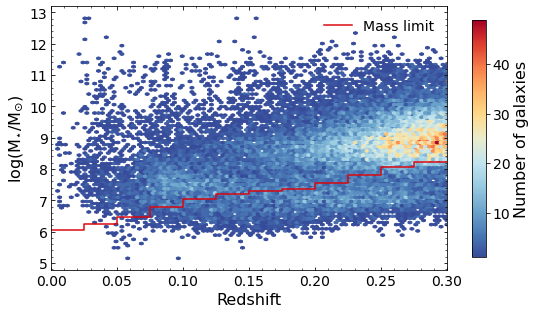
Figure 13: Stellar mass as a function of redshift. The number of galaxies in each mass-redshift bin is from low in blue to high in red. The mass limits calculated following Sect. 2.4 are shown as a red line.

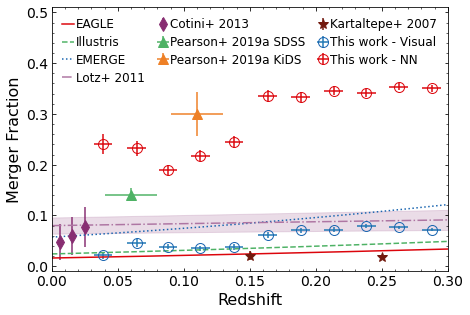
Figure 14: Merger fraction from the neural networks (red circles) and visual classification (blue circles) as a function of redshift. The merger fraction of the visually confirmed galaxies rises out to $z\approx 0.238$ before falling slightly. The error on the redshift is the standard deviation of the redshift within the redshift bin. The error on the merger fraction is the statistical error. Merger fractions from Cotini et al. (2013, purple diamonds), Pearson et al. (2019a, green and orange triangles), Kartaltepe et al. (2007, brown stars) and Lotz et al. (2011, dot-dashed purple line) are also shown along with the merger fraction trend from the EAGLE simulation (Qu et al. 2017, solid red line), Illustris simulation (Rodriguez-Gomez et al. 2015, dashed green line), and the pair fraction trend from the EMERGE simulation (O’Leary et al. 2021, dotted blue line).

An increasing merger fraction with redshift is consistent with other observational works. Using mergers identified by a CNN, Pearson et al. (2019a) find an increasing merger fraction as redshift increases, over $0.0<z<4.0$ using data from the Sloan Digital Sky Survey (York et al. 2000), KiDS and the Cosmic Assembly Near-infrared Deep Extragalactic Legacy Survey (Grogin et al. 2011; Koekemoer et al. 2011). An increase in the merger fraction with redshift is also seen with close pairs, galaxies with projected separations between 5 and 20 kpc, from $z=0.1$ to $z=1.2$ Kartaltepe et al. (2007). Using non-parametric statistics, Cotini et al. (2013) also find that the merger fraction increases with redshift at $z<0.03$. Similar results were found by Lotz et al. (2011), finding that the fraction of mergers and the fraction of close pair galaxies increases with redshift. Lotz et al. (2011) use a Gini-M₂₀ cut, asymmetry cut and select close pairs in Hubble Space Telescope data for galaxies with stellar masses above $10^{10}$ M_⊙.

We converted the merger rates of Lotz et al. (2011) into a merger fraction using their merger observability timescale of 0.2 Gyr for comparison with our results. We present their extrapolation to lower redshifts used in this work in Fig. 14 as the dot-dashed purple line, with their errors shown by the purple shaded region. At higher redshifts, the visually selected mergers are in agreement with the Lotz et al. (2011) merger fractions. At lower redshifts, the visually selected merger fraction is lower than that of Lotz et al. (2011). This may be due to the extrapolation required to reach these lower redshifts as the lowest redshift data point of Lotz et al. (2011) is at $z=0.3$. The observability timescale of Lotz et al. (2011) has slight redshift dependence which is not presented in the paper. Thus the use of constant timescale may be causing an increase in the Lotz et al. (2011) merger fraction presented here at lower redshifts. The merger candidate fraction is much higher than the Lotz et al. (2011) merger fraction. As we expect the merger candidates to be contaminated with a large number of non-mergers, this is expected.

Pearson et al. (2019a) has a much higher merger fraction than this work. This is likely a result of their pure CNN identification of galaxy mergers leaving many false merger detections in the merger sample. This will increase the merger fraction due to the prevalence of non-merging galaxies in the Universe compared to merging galaxies, hence there being more false merger detections than false non-merger detections. Indeed, the merger fraction from the KiDS sample in Pearson et al. (2019a) is consistent with the merger candidate fraction found by the neural network in this work, before visual confirmation. This consistency between the merger fractions found only with neural networks and these fractions being much larger than the visually selected merger fractions is a strong indication that merger identifications from current neural networks are highly contaminated with non-mergers.

The merger fractions of Cotini et al. (2013) are larger than the visually inspected merger fractions found in this work. The mergers presented in Cotini et al. (2013) have been visually checked, like in this work, so there are unlikely to be misclassified non-mergers. However, the size of the merger and non-merger samples are small, a few tens of non-mergers and a few mergers, so these fractions may suffer from low number statistics and so have large uncertainties as seen in Fig. 14. Kartaltepe et al. (2007) find merger fractions that are lower than this work, as can be seen in Fig. 14. As Kartaltepe et al. (2007) use close pairs, it is possible that earlier stage mergers are missed that the hybrid neural-network - human classification can find. To add to this, the close pair method misses mergers that are coalescence and post-coalescence which can be detected by the method presented in this work. As a result, it would be expected that the merger fractions presented here are larger than those in Kartaltepe et al. (2007).

Simulations also provide similar results. O’Leary et al. (2021) find the merger fraction increasing with redshift, at least at $z<1$, in the EMERGE cosmological simulation (Moster et al. 2018). This is also seen in the Illustris (Vogelsberger et al. 2014; Rodriguez-Gomez et al. 2015) and the Evolution and Assembly of Galaxies and their Environments (EAGLE; Schaye et al. 2015; Qu et al. 2017) hydrodynamical, cosmological simulations. However, the Horizon-AGN cosmological simulation (Dubois et al. 2014) finds no evolution of the merger fraction with redshift (Kaviraj et al. 2015).

The results presented in this paper show similar merger fractions to the EAGLE results for galaxies with stellar masses above 10¹⁰ M_⊙, at the lower redshifts presented in this work. At higher redshifts we find higher merger fractions than EAGLE. Higher merger fractions than EAGLE are expected. As our mass limits are lower than EAGLE at all redshifts, the largest mass limit in this work is less than 10⁹ M_⊙, we expect to find higher merger fractions (Stott et al. 2013). This is likely due to a greater fraction of lower mass galaxies are undergoing a merger compared to higher mass galaxies (Stott et al. 2013; Casteels et al. 2014; Wang et al. 2020). If the redshift evolution of the merger fraction in EAGLE and the visually selected mergers in this work were the same, it would be expected that the merger fraction of EAGLE and this work would converge towards higher masses, where the mass limit of this work becomes closer to that of EAGLE. As the opposite is seen, we find a faster increase in merger fraction with redshift compared to EAGLE if the same mass limits are used.

The Illustris simulation shows a similar merger fraction trend to the EAGLE simulation. Using the merger rate given by Rodriguez-Gomez et al. (2015) and assuming a merger ratio of 1/4 and a descendant mass of 10¹⁰ M_⊙, the merger rate is converted to a merger fraction by assuming an average observational timescale (T_obs) of 0.65 Gyr (Lotz et al. 2011). The Illustris merger fraction is consistent with the visually selected merger fraction at $z<0.15$. The visually selected merger fraction increases at a faster rate with redshift than the Illustris merger fraction and so the visually selected merger fraction rises above the Illustris merger fraction at $z>0.15$.

The EMERGE simulation finds a larger pair fraction than the visually selected merger fraction. In Fig. 14, we show the pair fraction from O’Leary et al. (2021) for simulated galaxy pairs with M${}_{\star}\geq 10^{10.3}$ M_☉ and projected distances between 5 and 50 kpc. As with the Illustris merger rate, the EMERGE merger rate has been multiplied by a T_obs of 0.65 Gyr to get the merger fraction. The EMERGE merger fraction is slightly larger than the visually selected merger fraction of this work, as can be seen in Fig. 14. However, the merger rate derived in O’Leary et al. (2021) does not apply a correction factor to account for not all galaxy pairs resulting in a merger. If a typical correction factor of 0.6 is applied (e.g. Conselice 2014), the EMERGE merger fraction is in good agreement with the visually selected merger fraction of this work. On the other hand, as pair samples miss post-coalescence galaxies, approximately half of all mergers, the EMERGE pair fraction as presented in O’Leary et al. (2021) is likely to be close to the true merger fraction of pre and post-merger galaxies. This is a result of the factor of 0.6 reduction not applied in O’Leary et al. (2021) being almost entirely offset by the approximate factor of 2 needed to account for the missing post-coalescence galaxies.

The comparisons with other works presented here are not exhaustive. There is a wealth of similar studies onto the merger fraction and merger rates in the Universe from a number of different surveys and data sources. They do, however, typically all indicate that the merger fraction increases with redshift, although the evolution with redshift does differ (e.g. Patton et al. 2002; Lin et al. 2004; de Ravel et al. 2009; López-Sanjuan et al. 2013; Casteels et al. 2014; Mundy et al. 2017; Ferreira et al. 2020). Moreover, Conselice et al. (2008) has an increasing merger fraction at lower redshifts but a decreasing fraction at high redshifts of $z\gtrapprox 2.5$.

5.3 Star-formation Enhancement

A second simple application of the catalogue allows the study of the star-formation enhancement, or lack thereof, due to galaxy mergers. For this, we compared the SFRs in the merger candidates and visually verified mergers with the SFRs in a control sample for star-forming galaxies.

Star-forming galaxies were selected based on their position relative to the galaxy main-sequence (MS), a tight correlation between the M_⋆ and SFR of star-forming galaxies (e.g. Brinchmann et al. 2004; Noeske et al. 2007; Elbaz et al. 2007; Speagle et al. 2014). We use the redshift dependent main-sequence of Pearson et al. (2018) at $z=0.24$ (orange line in Fig.15), the mean redshift of the mass complete sample defined in Sect. 5.2. The empirical scatter in this MS is $\sigma_{MS}=0.23$ dex. We consider galaxies above MS$-3\sigma_{MS}$ as part of the MS (red line in Fig. 15).

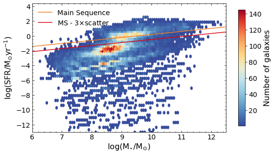
Figure 15: M_⋆-SFR plane for the galaxies classified by the neural networks. The number of galaxies in each M_⋆-SFR bin is from low in blue to high in red. The orange line indicates the Pearson et al. (2018) main-sequence at $z=0.24$ while the red line indicated three times the scatter below the main-sequence. Galaxies are classified as star-forming if they lie above the red line.

The control galaxies were selected from the non-merging samples, defined as galaxies with $\texttt{frac\_merger}<0.5$ for both the merger candidates and the visually selected mergers. For each merger (candidate), non-merging galaxies within 0.05 dex in M_⋆ and 0.005 in redshift were identified. Where at least one matching non-merger was found, each merger (candidate) was assigned a unique non-merger control. If no match was found, the matching distance was then increased by 0.05 dex in M_⋆ and 0.005 in redshift and the matching process repeated for any unmatched merging galaxies. The matching distance was repeatedly increased until the M_⋆ matching distance was over 0.3 dex or the redshift matching distance was over 0.05, the typical weighted dispersion of the photometric redshifts. Any merger (candidates) that had not been matched were then removed. Matching was done independently for the merger candidates and visually confirmed mergers. This process resulted in 2 905 of the 3 342 mass complete merger candidates and 801 of the 803 mass complete mergers having a matched control galaxy. The mass and redshift distributions for the merger candidates, mergers and their respective controls are shown in Fig. 16. The environment in which a galaxy lies, for example in a group, cluster or the field, can influence the SFR of a galaxy independent of if the galaxy is interacting or not, with high density regions having lower typical SFR (e.g. Lewis et al. 2002; Peng et al. 2010; Vázquez-Mata et al. 2020). For this work, the envirnoment in which the galaxy mergers and non-merger controlls lie was not considered when matching mergers with thier controlls.

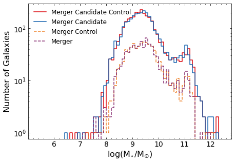
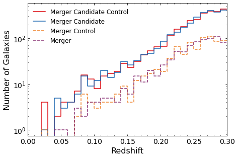
Figure 16: Stellar mass (left panel) and redshift (right panel) distributions for merger candidates (blue) and visually confirmed mergers (dashed purple) and their selected non-merging control galaxies (red and dashed orange for candidate and visually confirmed merger controls, respectively).

We find that for the merger candidates, the SFR of the control sample is only slightly lower than that of the merger candidate sample. Here we subtract the log(SFR/M_⊙yr^-1) of the control galaxies from the log(SFR/M_⊙yr^-1) of their matched merger candidate. The average of these differences is

$$\Delta\log(\mathrm{SFR}/M_{\odot}yr^{-1})=0.071\pm 0.014\leavevmode\nobreak\ \mathrm{dex}$$ (4)

with a sample standard deviation in $\Delta\log(\mathrm{SFR}/M_{\odot}yr^{-1})$ of

$$\sigma\Delta\log(\mathrm{SFR}/M_{\odot}yr^{-1})=0.733\pm 0.010\leavevmode\nobreak\ \mathrm{dex}.$$ (5)

The errors on $\sigma\Delta\log(\mathrm{SFR}/M_{\odot}yr^{-1})$ are the standard error for the standard deviation. Thus, the average SFR enhancement is in 5$\sigma$ tension of being zero. The average enhancement of the visually confirmed merger sample, derived in the same manner, is smaller than that of the merger candidates, with an average change to log(SFR/M_⊙yr^-1) being

$$\Delta\log(\mathrm{SFR}/M_{\odot}yr^{-1})=0.040\pm 0.025\leavevmode\nobreak\ \mathrm{dex}$$ (6)

and a sample standard deviation of

$$\sigma\Delta\log(\mathrm{SFR}/M_{\odot}yr^{-1})=0.696\pm 0.017\leavevmode\nobreak\ \mathrm{dex}.$$ (7)

For the visually selected mergers, therefore, the average enhancement is in 1$\sigma$ tension of being zero.

We know that the merger candidate sample is contaminated with non-mergers and the visually selected sample is also likely to be contaminated. If non-mergers have a lower SFR than merging galaxies, this contamination will act to reduce the SFR enhancement seen when comparing the mergers with non-mergers. The merger candidate and visually confirmed samples are likely to have a large fraction of widely separated galaxies. This is a result of widely separated galaxies being easier to identify by eye, and the training sample being based on visual selection and the visual confirmation being visual by design. Closely separated galaxies may show more merger-like features, but two very close galactic cores can be indistinguishable from a single galactic core. This makes the choice between a merging galaxy or an irregular galaxy difficult. More closely separated galaxies are more likely to have higher SFRs (e.g. Davies et al. 2015; Moreno et al. 2019) so a high fraction of widely spaced galaxies can weaken any SFR enhancement. To add to this, if our control sample is primarily selected from lower density environments while the mergers are in higher density environments, this will act to suppress the apparent SFR enhancement for the merging systems. These factors could be combining to give such a marginal enhancement in both samples.

These results are qualitatively in line with other works in that the enhancement we see to SFR is less than a factor of two. The low SFR enhancement is consistent with Silva et al. (2018), who find no significant SFR enhancement in merging galaxies when compared to non-mergers. Knapen et al. (2015) find a typical increase in SFR by up to a factor of 1.9 for the most highly interacting and closest pair galaxies with a reduction in SFR enhancement as the galaxies are more wideley separated. Hwang et al. (2011) also see an increase in SFR of a factor of approximately 2 for merging galaxies when compared to non-merging counterparts. Ellison et al. (2013) find an increase in SFR by a factor of 2 for pre-merger galaxies and 3.5 for post mergers. They also find that the enhancement is greater for galaxy pairs with smaller separation. In this work, we do not distinguish between pre and post-mergers nor do we determine the separation of the galaxy pairs. However, as the enhancement of the merger galaxies is much less than the 3.5 seen for post-merger galaxies in Ellison et al. (2013), it suggests that the sample of galaxies herein identified are primarily pre-merger galaxies. The visual confirmation of the galaxy mergers did not directly record the type of merger, pre-merger or post-merger, but a brief reinspection shows the identified galaxies are more likely to be pre-merger systems. The visual identifier WJP is not biased towards pre-merger or post-merger systems while LES has a slight bias towards post-merger systems, see Appendix B, suggesting the greater number of pre-mergers is not a result of visual classifier selection bias. The larger SFR enhancement seen in Ellison et al. (2013) may be a result of their controlling for environment. The environment controlled sample of Ellison et al. (2013) will not suffer from the potential environmental influence that may be influencing our results, as noted above.

The work of Pearson et al. (2019a) provides an interesting comparison to this work. Both this work and that of Pearson et al. (2019a) identify galaxy mergers using neural networks, a CNN in Pearson et al. (2019a) and a CNN-FCN-human hybrid here. Pearson et al. (2019a) find a typical enhancement to SFR of a factor of $1.15\pm 0.12$ while we find an enhancement of a factor of $1.178\pm 0.065$ for the merger candidates, the closest comparison. Evidently, these two values are consistent within the standard errors in the means. Both the Pearson et al. (2019a) merger sample and the merger candidates of this work are likely to be contaminated with non-merging galaxies. If mergers are typically of higher SFR than non-mergers it would be expected that the increase in SFR for a merger sample with fewer contaminants would have a larger change in SFR. However, this is not what is seen in this work, indeed a smaller enhancement to SFR is seen with the visually confirmed merger sample. Thus, it may be expected that cleaning the Pearson et al. (2019a) merger sample may similarly see a smaller SFR enhancement. We note, however, that Pearson et al. (2019a) compare the average SFR of their mergers with the average SFR of the non-mergers while here we compare the difference in SFR between a merger and its matched control.

6 Summary

In this paper, we present a catalogue of galaxy mergers in the North Ecliptic Pole field using optical data from the Hyper Suprime-Cam. The merger identification is a hybrid of automated and human classification: a neural network is used to identify merger candidates which are then visually inspected. The neural networks used a combination of both images and morphological parameters, which was found to provide better results than just images or morphological parameters alone. From the hybrid approach for merger identification, the final catalogue contains 2 109 merging galaxies out of a total of 34 264 galaxies with redshifts between 0.0 and 0.3.

Studying the networks and how they classify the galaxies, it appears that both the networks will miss-classify galaxies as merging that have a companion that is close in projection but not physically associated. Both networks appear to primarily rely on the morphological parameters for classification with parameters that examine the asymmetry of the light distribution being a key component.

As test applications of the catalogue, we performed an analysis of the merger fraction as a function of redshift and examine the SFR enhancement due to galaxy mergers. We find that the evolution of the merger fraction is qualitatively consistent with merger fraction evolutions found in other observational surveys as well as cosmological simulations. For the SFR enhancement, we find a mild increase by a factor of $1.178\pm 0.065$ for the merger candidates and a factor of $1.096\pm 0.063$ for the visually confirmed mergers, consistent with other works.

The resulting catalogue is well placed to be exploited for further use within the NEP field. It is also in a prime position to be used as a training set for the upcoming Euclid Northern deep field. Due to the scale of the upcoming surveys, such a catalogue could prove to be invaluable as a training sample for automated merger detection over larger regions of the sky.

Appendix A CNN performance definitions

The terms used to describe the performance of the neural networks presented in this work may be an alternate nomenclature to other works or may be unfamiliar. To avoid confusion we present the definitions used in this work in Table 7.

Table 7: Terms used when describing the performance of neural networks from Pearson et al. (2019b)

Term	Definition
True Positive (TP)	An object known to be a merger that is identified by a network as a merger.
False Positive (FP)	An object known to be a non-merger that is identified by a network as a merger.
True Negative (TN)	An object known to be a non-merger that is identified by a network as a non-merger.
False Negative (FN)	An object known to be a merger that is identified by a network as a non-merger.
Recall	Fraction of objects correctly identified by a network as a merger with respect to the total number of objects classified in the catalogues as mergers.	TP / (TP+FN)
Specificity	Fraction of objects correctly identified by a network as a non-merger with respect to the total number of objects classified in the catalogues as non-mergers.	TN / (TN+FP)
Precision	Fraction of objects correctly identified by a network as a merger with respect to the total number of objects identified by a network as a merger.	TP / (TP+FP)
Negative Predictive Value (NPV)	Fraction of objects correctly identified by a network as a non-merger with respect to the total number of objects identified by a network as a non-merger.	TN / (TN+FN)
Accuracy	Fraction of objects, both merger and non-merger, correctly identified by a network.	(TP+TN) / (TP+FP+TN+FN)

Appendix B Visual inspection performance

To check the performance of the two authors’ merger identification, images of mergers and non-mergers from the Illustris TNG simulation (Marinacci et al. 2018; Naiman et al. 2018; Nelson et al. 2018; Pillepich et al. 2018; Springel et al. 2018; Nelson et al. 2019) were used. A sample of 100 major merger galaxies were selected, along with a further 100 non-mergers, from snapshot 87 ($z=0.15$). Here, a major merger is defined to have merged in the last 500 Myr or will merge in the next 1000 Myr and have a mass ratio of $<4:1$ (Wang et al. 2020). This mass ratio is derived from the stellar masses of the two merging galaxies at the snapshot when the secondary galaxy reached its maximum stellar mass (Rodriguez-Gomez et al. 2015). The simulated galaxies were then convolved with the point-spread function of the HSC-NEP images before being embedded into the HSC-NEP images to add realistic noise and chance projections. The position in the image where the simulated galaxies were embedded were selected such that there were no sources in the HSC-NEP catalogue within 10 arcsec (64 pixels). These mock galaxy observations were then classified by WJP and LES, with neither knowing if the galaxy was truly a merger or non-merger, only that the sample had an equal number of each. The results of the performance test can be found in Table 8.

Table 8: Performance statistics of WJP and LES classifying simulated observations of merging and non-merging galaxies.

Statistic	WJP	LES
Accuracy	0.620	0.630
Recall	0.450	0.440
Precision	0.682	0.710
Specificity	0.790	0.820
NPV	0.590	0.594

As can be seen, the performance of WJP and LES is lower than that of the neural networks presented in this work but both are similar. WJP has fewer FP than LES (21 compared to 18) but also has more TP (45 compared to 41). However, both authors correctly identify fewer than half of the merging galaxies. For the FN, there is no clear trend with time before or after the merger, as shown in Fig. 17. WJP has a larger fraction of missed mergers that are close to the merger event (here defined as the snapshot when two galaxies are tracked as one in the simulation) than LES while LES has a larger fraction of missed mergers with longer times until the merger event will take place. Thus WJP is likely to miss merging galaxies that are physically close to one another or have just merged. On the other hand, LES is likely to miss galaxies that are at the early stages of a merger.

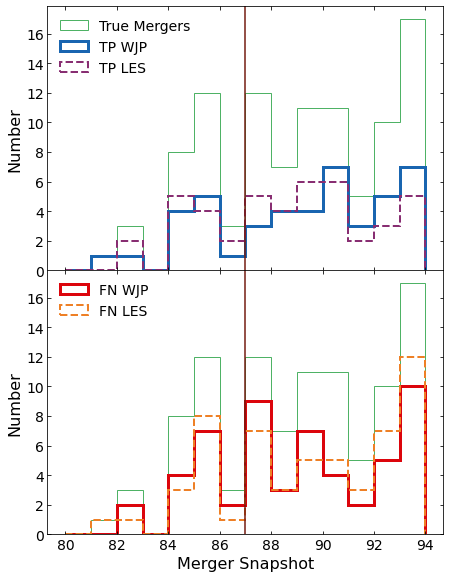
Figure 17: Plot of correctly and incorrectly identified images of simulated mergers as a function of snapshot when the merger occurred. The blue and red lines indicate the TP and FN, respectively, classified by WJP while the purple and orange dashed lines indicate the TP and FN, respectively, classified by LES. The Green line indicates the total number of mergers used from Illustris TNG while the vertical brown line indicates the snapshot of observation (87, $z=0.15$).

Appendix C Examples of differet galaxy classification

Further to the discussion in the main body of the paper, in this appendix we study, in more detail, if the neural network has been inadvertantly trained to identify structured and unstructured galaxies. To this end, we present 16 randomly selected non-mergers in Fig. 18 and 16 randomly selected merger candidates (both TP and FP) in Fig. 19. While the non-mergers presented in Fig. 18 are predominantly unstructured galaxies, the same is also true of the merger candidates presented in Fig. 19. Examples of structured non-mergers are presented in Fig. 6 above. The images of unstructured merger candidates do typically contain other galaxies or stars in close projection, although later may be found to be unassociated during visual inspection. If the neural networks had been trained to identify structured and unstructured galaxies, very few merger candidates would be expected to not have structure regardless of whether there are other objects in close projection. As this is not the case, we conclude that the networks are indeed identifying mergers and non-mergers as intended. For comparison, we also present 16 randomly selected visually confirmed mergers in Fig. 20.

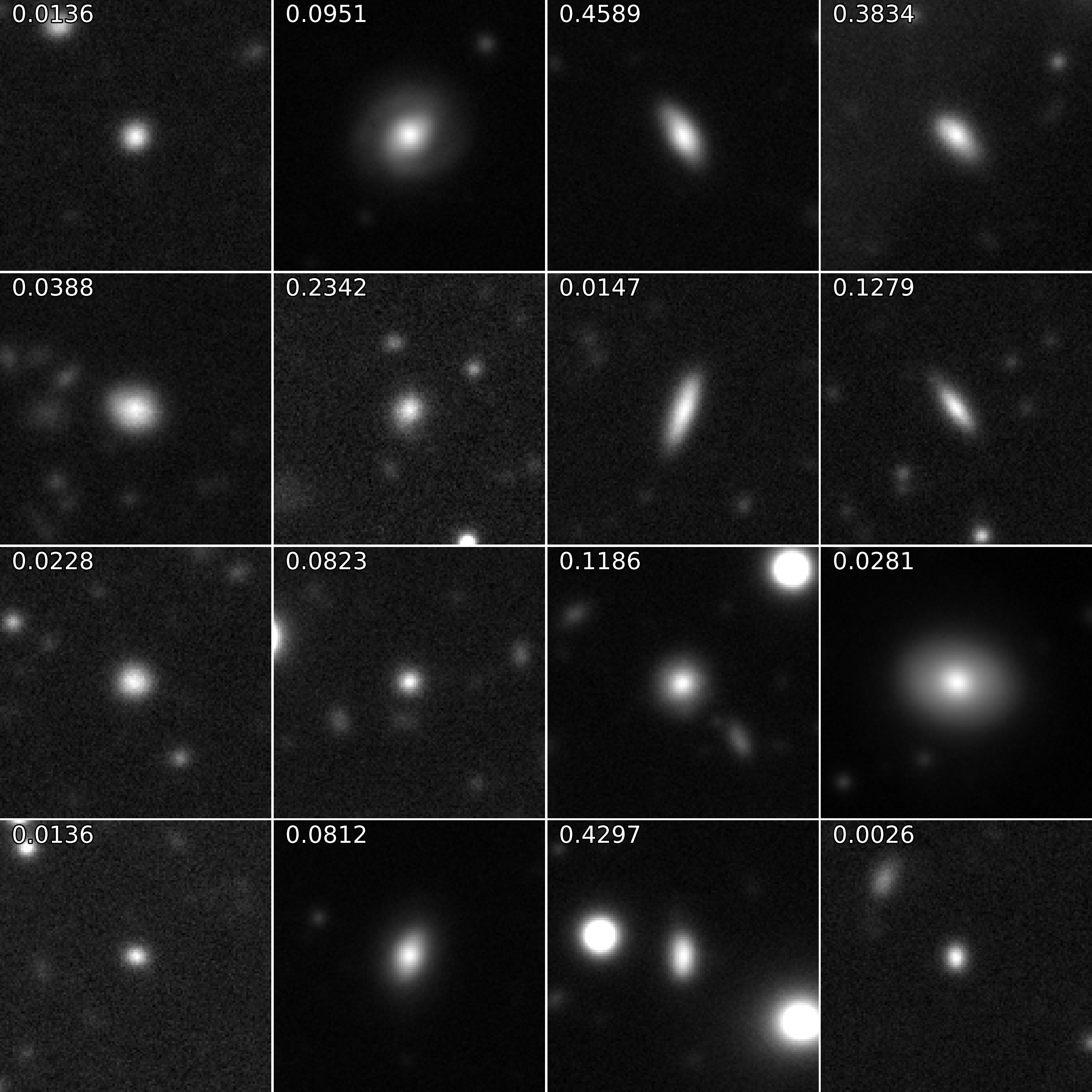
Figure 18: Sixteen randomly selected galaxies identified as non-mergers by the neural networks with frac_merger in the upper left corner of the image.

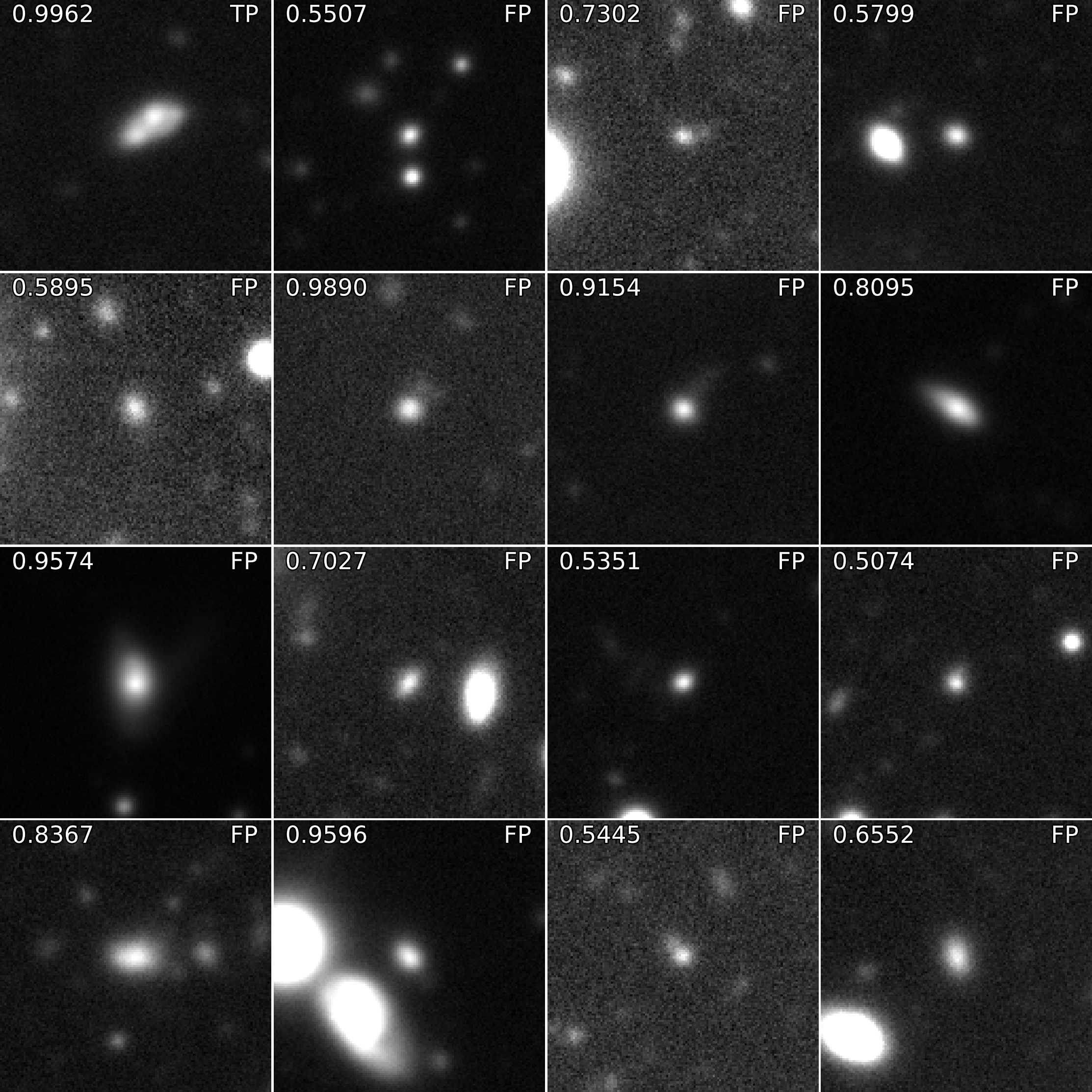
Figure 19: Sixteen randomly selected galaxies identified as mergers by the neural networks with frac_merger in the upper left corner of the image and if they are TP or FP in the top right corner.

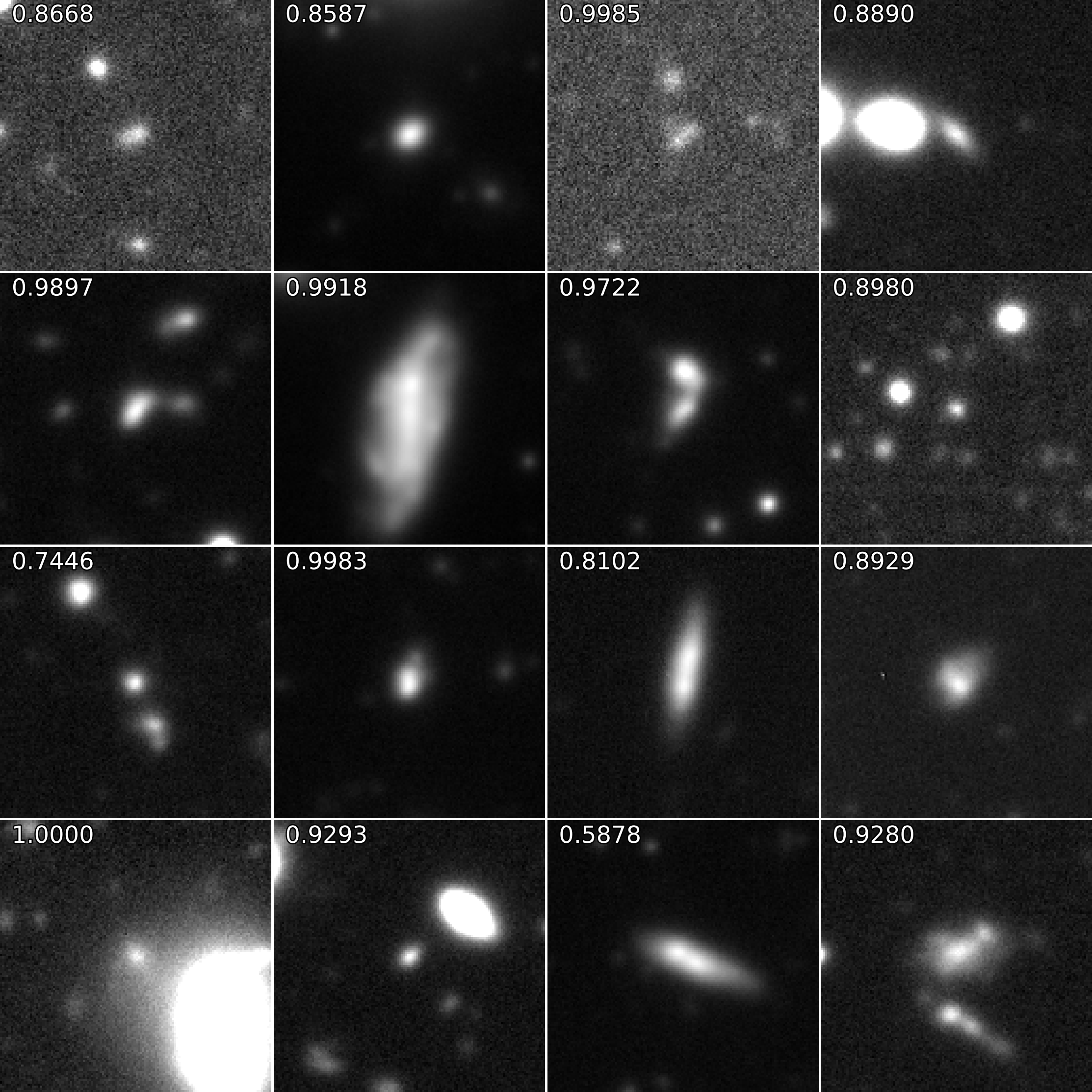
Figure 20: Sixteen randomly selected galaxies visually confirmed to be mergers with frac_merger in the upper left corner of the image.