The duo Fenchel-Young divergence

Abstract

By calculating the Kullback-Leibler divergence between two probability measures belonging to different exponential families, we end up with a formula that generalizes the ordinary Fenchel-Young divergence. Inspired by this formula, we define the duo Fenchel-Young divergence and reports a majorization condition on its pair of generators which guarantees that this divergence is always non-negative. The duo Fenchel-Young divergence is also equivalent to a duo Bregman divergence. We show the use of these duo divergences by calculating the Kullback-Leibler divergence between densities of nested exponential families, and report a formula for the Kullback-Leibler divergence between truncated normal distributions. Finally, we prove that the skewed Bhattacharyya distance between nested exponential families amounts to an equivalent skewed duo Jensen divergence.

Keywords: exponential family; statistical divergence; truncated normal distributions.

1 Introduction

1.1 Exponential families

Let $(\mathcal{X},\Sigma)$ be a measurable space, and consider a regular minimal exponential family [28] $\mathcal{E}$ of probability measures $P_{\theta}$ all dominated by a base measure $\mu$ ($P_{\theta}\ll\mu$):

$$\mathcal{E}=\{P_{\theta}\ :\ \theta\in\Theta\}.$$

The Radon-Nikodym derivatives of the probability measures $P_{\theta}$ with respect to $\mu$ can be written canonically as

$$p_{\theta}(x)=\frac{\mathrm{d}P_{\theta}}{\mathrm{d}\mu}(x)=\exp\left(\theta^{\top}t(x)-F(\theta)+k(x)\right),$$

where $\theta$ denotes the natural parameter, $t(x)$ the sufficient statistic, and $F(\theta)$ the log-normalizer [28] (or cumulant function). The optional auxiliary term $k(x)$ allows to change the base measure $\mu$ into the measure $\nu$ such that $\frac{\mathrm{d}\nu}{\mathrm{d}\mu}(x)=e^{k(x)}$. The distributions $P_{\theta}$ of the exponential family $\mathcal{E}$ can be interpreted as distributions obtained by tilting the base measure $\mu$ [12]. Thus when $t(x)=x$, these natural exponential families [28] are also called tilted exponential families [15] in the literature.

1.2 Kullback-Leibler divergence between exponential family distributions

For two $\sigma$-finite probability measures $P$ and $Q$ on $(\mathcal{X},\Sigma)$ such that $P$ is dominated by $Q$ ($P\ll Q$), the Kullback-Leibler divergence between $P$ and $Q$ is defined by

$$D_{\mathrm{KL}}[P:Q]=\int_{\mathcal{X}}\log\frac{\mathrm{d}P}{\mathrm{d}Q}\,\mathrm{d}P=E_{P}\left[\log\frac{\mathrm{d}P}{\mathrm{d}Q}\right].$$

When $P\not\ll Q$, we set $D_{\mathrm{KL}}[P:Q]=+\infty$. Gibbs’ inequality [9] $D_{\mathrm{KL}}[P:Q]\geq 0$ shows that the KLD is always non-negative. The proof of Gibbs’ inequality relies on Jensen’s inequality and holds for the wide class of $f$-divergences [10] induced by convex generators $f(u)$:

$$I_{f}[P:Q]=\int_{\mathcal{X}}f\left(\frac{\mathrm{d}Q}{\mathrm{d}P}\right)\,\mathrm{d}P\geq f\left(\int_{\mathcal{X}}\frac{\mathrm{d}Q}{\mathrm{d}P}\,\mathrm{d}P\right)\geq f(1).$$

The KLD is a $f$-divergence for the convex generator $f(u)=-\log u$.

1.3 Kullback-Leibler divergence between exponential family densities

It is well-known that the KLD between two distributions $P_{\theta_{1}}$ and $P_{\theta_{2}}$ of $\mathcal{E}$ amounts to compute an equivalent Fenchel-Young divergence [3]:

$$D_{\mathrm{KL}}[P_{\theta_{1}}:P_{\theta_{2}}]=\int_{\mathcal{X}}p_{\theta_{1}}\log\frac{p_{\theta_{1}}}{p_{\theta_{2}}}\,\mathrm{d}\mu(x)=Y_{F,F^{*}}(\theta_{2},\eta_{1}),$$

where $\eta=\nabla F(\theta)=E_{P_{\theta}}[t(x)]$ is the moment parameter [28], and the Fenchel-Young divergence is defined for a pair of strictly convex conjugate functions [27] $F(\theta)$ and $F^{*}(\eta)$ related by the Legendre-Fenchel transform by

$$Y_{F,F^{*}}(\theta_{1},\eta_{2}):=F(\theta_{1})+F^{*}(\eta_{2})-\theta_{1}^{\top}\eta_{2}.$$

Amari (1985) first introduced this formula as the canonical divergence of dually flat spaces in information geometry [2] (Eq. 3.21), and proved that the Fenchel-Young divergence is obtained as the KLD between densities belonging to a same exponential family [2] (Theorem 3.7). Azoury and Warmuth expressed the KLD $D_{\mathrm{KL}}[P_{\theta_{1}}:P_{\theta_{2}}]$ using dual Bregman divergences in [3] (2001):

$$D_{\mathrm{KL}}[P_{\theta_{1}}:P_{\theta_{2}}]=B_{F}(\theta_{2}:\theta_{1})=B_{F^{*}}(\eta_{1}:\eta_{2}),$$

where a Bregman divergence [7] $B_{F}(\theta_{1}:\theta_{2})$ is defined for a strictly convex and differentiable generator $F(\theta)$ by:

$$B_{F}(\theta_{1}:\theta_{2}):=F(\theta_{1})-F(\theta_{2})-(\theta_{1}-\theta_{2})^{\top}\nabla F(\theta_{2}).$$

Acharyya termed the divergence $Y_{F,F^{*}}$ the Fenchel-Young divergence in his PhD thesis [1] (2013), and Blondel et al. called them Fenchel-Young losses (2020) in the context of machine learning [6] (Eq. 9 in Definition 2). It was also called by the author the Legendre-Fenchel divergence in [19]. The Fenchel-Young divergence stems from the Fenchel-Young inequality [27]:

$$F(\theta_{1})+F^{*}(\eta_{2})\geq\theta_{1}^{\top}\eta_{2},$$

with equality iff. $\eta_{2}=\nabla F(\theta_{1})$. Figure 1 visualizes the 1D Fenchel–Young divergence and gives a geometric proof that $Y_{F,F^{*}}(\theta_{1},\eta_{2})\geq 0$ with equality if and only if $\eta_{2}=F^{\prime}(\theta_{1})$.

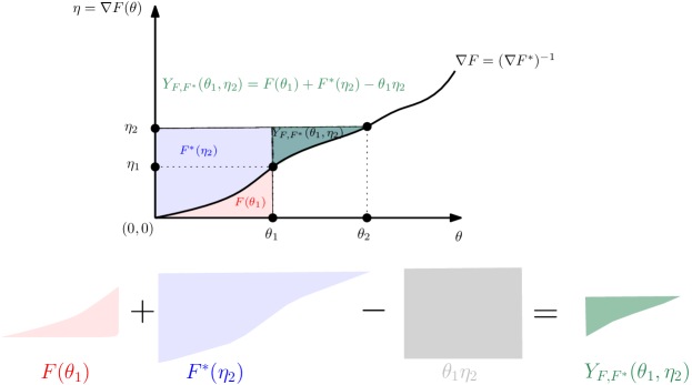
Figure 1: Visualizing the Fenchel–Young divergence.

The symmetrized Kullback-Leibler divergence $D_{J}[P_{\theta_{1}}:P_{\theta_{2}}]$ between two distributions $P_{\theta_{1}}$ and $P_{\theta_{2}}$ of $\mathcal{E}$ is called the Jeffreys’ divergence [17] and amounts to a symmetrized Bregman divergence [23]:

$$D_{J}[P_{\theta_{1}}:P_{\theta_{2}}] = D_{\mathrm{KL}}[P_{\theta_{1}}:P_{\theta_{2}}]+D_{\mathrm{KL}}[P_{\theta_{2}}:P_{\theta_{1}}],$$ (1)

$$= B_{F}(\theta_{2}:\theta_{1})+B_{F}(\theta_{1}:\theta_{2}),$$ (2)

$$= (\theta_{2}-\theta_{1})^{\top}(\eta_{2}-\eta_{1}):=S_{F}(\theta_{1},\theta_{2}).$$ (3)

Notice that the Bregman divergence $B_{F}(\theta_{1}:\theta_{2})$ can also be interpreted as a surface area:

$$B_{F}(\theta_{1}:\theta_{2})=\int_{\theta_{2}}^{\theta_{1}}(F^{\prime}(\theta)-F^{\prime}(\theta_{2}))\mathrm{d}\theta.$$ (4)

Figure 2 illustrates the sided and symmetrized Bregman divergences.

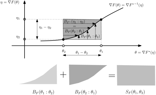
Figure 2: Visualizing the sided and symmetrized Bregman divergences.

1.4 Contributions and paper outline

We recall in §2 the formula obtained for the Kullback-Leibler divergence between two exponential family densities equivalent to each other [20] (Eq. 5). Inspired by this formula, we give a definition of the duo Fenchel-Young divergence induced by a pair of strictly convex functions $F_{1}$ and $F_{2}$ (Definition 1) in §3, and proves that the divergence is always non-negative provided that $F_{1}$ upper bounds $F_{2}$. We then define the duo Bregman divergence (Definition 2) corresponding to the duo Fenchel-Young divergence. In §4, we show that the Kullback-Leibler divergence between a truncated density and a density of a same parametric exponential family amounts to a duo Fenchel-Young divergence or equivalently to a Bregman divergence on swapped parameters (Theorem 1). As an example, we report a formula for the Kullback-Leibler divergence between truncated normal distributions (Example 6). In §5, we further consider the skewed Bhattacharyya distance between nested exponential family densities and prove that it amounts to a duo Jensen divergence (Theorem 2). Finally, we conclude in §7.

2 Kullback-Leibler divergence between different exponential families

Consider now two exponential families [28] $\mathcal{P}$ and $\mathcal{Q}$ defined by their Radon-Nikodym derivatives with respect to two positive measures $\mu_{\mathcal{P}}$ and $\mu_{\mathcal{Q}}$ on $(\mathcal{X},\Sigma)$:

$$\mathcal{P} = \left\{P_{\theta}\ :\ \theta\in\Theta\right\},$$

$$\mathcal{Q} = \left\{Q_{\theta^{\prime}}\ :\ \theta^{\prime}\in\Theta^{\prime}\right\}.$$

The corresponding natural parameter spaces are

$$\Theta = \left\{\theta\in\mathbb{R}^{D}\ :\ \int_{\mathcal{X}}\exp(\theta^{\top}t_{\mathcal{P}}(x)+k_{\mathcal{P}}(x))\,\mathrm{d}\mu_{\mathcal{P}}(x)<\infty\right\},$$

$$\Theta^{\prime} = \left\{\theta^{\prime}\in\mathbb{R}^{D^{\prime}}\ :\ \int_{\mathcal{X}}\exp({\theta^{\prime}}^{\top}t_{\mathcal{Q}}(x)+k_{\mathcal{Q}}(x))\,\mathrm{d}\mu_{\mathcal{Q}}(x)<\infty\right\},$$

The order of $\mathcal{P}$ is $D$, $t_{\mathcal{P}}(x)$ denotes the sufficient statistics of $P_{\theta}$, and $k_{\mathcal{P}}(x)$ is a term to adjust/tilt the base measure $\mu_{\mathcal{P}}$. Similarly, the order of $\mathcal{Q}$ is $D^{\prime}$, $t_{\mathcal{Q}}(x)$ denotes the sufficient statistics of $Q_{\theta^{\prime}}$, and $k_{\mathcal{Q}}(x)$ is an optional term to adjust the base measure $\mu_{\mathcal{Q}}$. Let $p_{\theta}$ and $q_{\theta^{\prime}}$ denote the Radon-Nikodym with respect to the measure $\mu_{\mathcal{P}}$ and $\mu_{\mathcal{Q}}$, respectively:

$$p_{\theta} = \frac{\mathrm{d}P_{\theta}}{\mathrm{d}\mu_{\mathcal{P}}}=\exp(\theta^{\top}t_{\mathcal{P}}(x)-F_{\mathcal{P}}(\theta)+k_{\mathcal{P}}(x)),$$

$$q_{\theta^{\prime}} = \frac{\mathrm{d}Q_{\theta^{\prime}}}{\mathrm{d}\mu_{\mathcal{Q}}}=\exp({\theta^{\prime}}^{\top}t_{\mathcal{Q}}(x)-F_{\mathcal{Q}}(\theta^{\prime})+k_{\mathcal{Q}}(x)),$$

where $F_{\mathcal{P}}(\theta)$ and $F_{\mathcal{Q}}(\theta^{\prime})$ denote the corresponding log-normalizers of $\mathcal{P}$ and $\mathcal{Q}$, respectively.

$$F_{\mathcal{P}}(\theta) = \log\left(\int\exp(\theta^{\top}t_{\mathcal{P}}(x)+k_{\mathcal{P}}(x))\,\mathrm{d}\mu_{\mathcal{P}}(x)\right),$$

$$F_{\mathcal{Q}}(\theta) = \log\left(\int\exp(\theta^{\top}t_{\mathcal{Q}}(x)+k_{\mathcal{Q}}(x))\,\mathrm{d}\mu_{\mathcal{Q}}(x)\right).$$

The functions $F_{\mathcal{P}}$ and $F_{\mathcal{Q}}$ are strictly convex and real analytic [28]. Hence, those functions are infinitely many times differentiable on their open natural parameter spaces.

Consider the KLD between $P_{\theta}\in\mathcal{P}$ and $Q_{\theta^{\prime}}\in\mathcal{Q}$ such that $\mu_{\mathcal{P}}=\mu_{\mathcal{Q}}$ (and hence $P_{\theta}\ll Q_{\theta^{\prime}}$). Then the KLD between $P_{\theta}$ and $Q_{\theta^{\prime}}$ was first considered in [20]:

$$D_{\mathrm{KL}}[P_{\theta}:Q_{\theta^{\prime}}] = E_{P}\left[\log\left(\frac{\mathrm{d}P_{\theta}}{\mathrm{d}Q_{\theta^{\prime}}}\right)\right],$$

$$= E_{P_{\theta}}\left[\left(\theta^{\top}t_{\mathcal{P}}(x)-{\theta^{\prime}}^{\top}t_{\mathcal{Q}}(x)-F_{\mathcal{P}}(\theta)+F_{\mathcal{Q}}(\theta^{\prime})+k_{\mathcal{P}}(x)-k_{\mathcal{Q}}(x)\right)\underbrace{\frac{\mathrm{d}\mu_{\mathcal{P}}}{\mathrm{d}\mu_{\mathcal{Q}}}}_{=1}\right],$$

$$= F_{\mathcal{Q}}(\theta^{\prime})-F_{\mathcal{P}}(\theta)+\theta^{\top}E_{P_{\theta}}[t_{\mathcal{P}}(x)]-{\theta^{\prime}}^{\top}E_{P_{\theta}}\left[t_{\mathcal{Q}}(x)\right]+E_{P_{\theta}}\left[k_{\mathcal{P}}(x)-k_{\mathcal{Q}}(x)\right].$$

Recall that the dual parameterization of an exponential family density $P_{\theta}$ is $P^{\eta}$ with $\eta=E_{P_{\theta}}[t_{\mathcal{P}}(x)]=\nabla F_{\mathcal{P}}(\theta)$ [28], and that the Fenchel-Young equality is $F(\theta)+F^{*}(\eta)=\theta^{\top}\eta$ for $\eta=\nabla F(\theta)$. Thus the KLD between $P_{\theta}$ and $Q_{\theta^{\prime}}$ can be rewritten as

$$\boxed{D_{\mathrm{KL}}[P_{\theta}:Q_{\theta^{\prime}}]=F_{\mathcal{Q}}(\theta^{\prime})+F_{\mathcal{P}}^{*}(\eta)-{\theta^{\prime}}^{\top}E_{P_{\theta}}\left[t_{\mathcal{Q}}(x)\right]+E_{P_{\theta}}\left[k_{\mathcal{P}}(x)-k_{\mathcal{Q}}(x)\right].}$$ (5)

This formula was reported in [20] and generalizes the Fenchel-Young divergence [1] obtained when $\mathcal{P}=\mathcal{Q}$ (with $t_{\mathcal{P}}(x)=t_{\mathcal{Q}}(x)$, $k_{\mathcal{P}}(x)=k_{\mathcal{Q}}(x)$, and $F(\theta)=F_{\mathcal{P}}(\theta)=F_{\mathcal{Q}}(\theta)$ and $F^{*}(\eta)=F_{\mathcal{P}}^{*}(\eta)=F_{\mathcal{Q}}^{*}(\eta)$).

The formula of Eq. 5 was illustrated in [20] with two examples: The KLD between Laplacian distributions and zero-centered Gaussian distributions, and the KLD between two Weibull distributions. Both these examples use the Lebesgue base measure for $\mu_{\mathcal{P}}$ and $\mu_{\mathcal{Q}}$.

Let us report another example which uses the counting measure as the base measure for $\mu_{\mathcal{P}}$ and $\mu_{\mathcal{Q}}$.

Example 1.

Consider the KLD between a Poisson probability mass function (pmf) and a geometric pmf. The canonical decomposition of the Poisson and geometric pmfs are summarized in Table 1. The KLD between a Poisson pmf $p_{\lambda}$ and a geometric pmf $q_{p}$ is equal to

$$D_{\mathrm{KL}}[P_{\lambda}:Q_{p}] = F_{\mathcal{Q}}(\theta^{\prime})+F_{\mathcal{P}}^{*}(\eta)-E_{P_{\theta}}[t_{\mathcal{Q}}(x)]\cdot\theta^{\prime}+E_{P_{\theta}}[k_{\mathcal{P}}(x)-k_{\mathcal{Q}}(x)],$$ (6)

$$= -\log p+\lambda\log\lambda-\lambda-\lambda\log(1-p)-E_{P_{\lambda}}[\log x!].$$ (7)

Since $E_{p_{\lambda}}[-\log x!]=-\sum_{k=0}^{\infty}e^{-\lambda}\frac{\lambda^{k}\log(k!)}{k!}$, we have

$$D_{\mathrm{KL}}[P_{\lambda}:Q_{p}]=-\log p+\lambda\log\frac{\lambda}{1-p}-\lambda-\sum_{k=0}^{\infty}e^{-\lambda}\frac{\lambda^{k}\log(k!)}{k!}$$

Notice that we can calculate the KLD between two geometric distributions $Q_{p_{1}}$ and $Q_{p_{2}}$ as

$$D_{\mathrm{KL}}[Q_{p_{1}}:Q_{p_{2}}] = B_{F_{\mathcal{Q}}}(\theta(p_{2}):\theta(p_{1})),$$

$$= F_{\mathcal{Q}}(\theta(p_{2}))-F_{\mathcal{Q}}(\theta(p_{1}))-(\theta(p_{2})-\theta(p_{1}))\eta(p_{1}),$$

We get:

$$D_{\mathrm{KL}}[Q_{p_{1}}:Q_{p_{2}}]=\log\left(\frac{p_{1}}{p_{2}}\right)-\left(1-\frac{1}{p_{1}}\right)\log\frac{1-p_{1}}{1-p_{2}}.$$

	Poisson family $\mathcal{P}$	Geometric family $\mathcal{Q}$
support	$\mathbb{N}\cup\{0\}$	$\mathbb{N}\cup\{0\}$
base measure	counting measure	counting measure
ordinary parameter	rate $\lambda>0$	success probability $p\in(0,1)$
pmf	$\frac{\lambda^{x}}{x!}\exp(-\lambda)$	$(1-p)^{x}p$
sufficient statistic	$t_{\mathcal{P}}(x)=x$	$t_{\mathcal{Q}}(x)=x$
natural parameter	$\theta(\lambda)=\log\lambda$	$\theta(p)=\log(1-p)$
cumulant function	$F_{\mathcal{P}}(\theta)=\exp(\theta)$	$F_{\mathcal{Q}}(\theta)=-\log(1-\exp(\theta))$
	$F_{\mathcal{P}}(\lambda)=\lambda$	$F_{\mathcal{Q}}(p)=-\log(p)$
auxiliary measure term	$k_{\mathcal{P}}(x)=-\log x!$	$k_{\mathcal{Q}}(x)=0$
moment parameter $\eta=E[t(x)]$	$\eta=\lambda$	$\eta=\frac{e^{\theta}}{1-e^{\theta}}=\frac{1}{p}-1$
negentropy (convex conjugate)	$F^{*}_{\mathcal{P}}(\eta(\lambda))=\lambda\log\lambda-\lambda$	$F^{*}_{\mathcal{Q}}(\eta(p))=\left(1-\frac{1}{p}\right)\log(1-p)+\log p$
($F^{*}(\eta)=\theta\cdot\eta-F(\theta)$)

Table 1: Canonical decomposition of the Poisson and the geometric discrete exponential families.

3 The duo Fenchel-Young divergence and its corresponding duo Bregman divergence

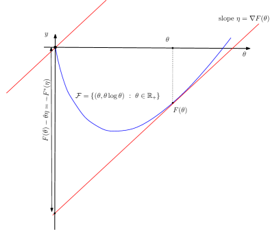
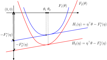
(a)	(b)

Figure 3: (a) Visual illustration of the Legendre-Fenchel transformation: $F^{*}(\eta)$ is measured as the vertical gap between the origin and the hyperplane of “slope” $\eta$ tangent at $F(\theta)$ evaluated at $\theta=0$. (b) The Legendre transforms $F_{1}^{*}(\eta)$ and $F_{1}^{*}(\eta)$ of two functions $F_{1}(\theta)$ and $F_{2}(\theta)$ such that $F_{1}(\theta)\geq F_{2}(\theta)$ reverses the dominance order: $F_{2}^{*}(\eta)\geq F_{1}^{*}(\eta)$.

Inspired by formula of Eq. 5, we shall define the duo Fenchel-Young divergence using a dominance condition on a pair $(F_{1}(\theta),F_{2}(\theta))$ of strictly convex generators:

Definition 1 (duo Fenchel-Young divergence).

Let $F_{1}(\theta)$ and $F_{2}(\theta)$ be two strictly convex functions such that $F_{1}(\theta)\geq F_{2}(\theta)$ for any $\theta\in\Theta_{12}=\mathrm{dom}(F_{1})\cap\mathrm{dom}(F_{2})$. Then the duo Fenchel-Young divergence $Y_{F_{1},F_{2}^{*}}(\theta,\eta^{\prime})$ is defined by

$$\boxed{Y_{F_{1},F_{2}^{*}}(\theta,\eta^{\prime}):=F_{1}(\theta)+F_{2}^{*}(\eta^{\prime})-\theta^{\top}\eta^{\prime}.}$$ (8)

When $F_{1}(\theta)=F_{2}(\theta)=:F(\theta)$, we have $F_{1}^{*}(\eta)=F_{2}^{*}(\eta)=:F^{*}(\eta)$, and we retrieve the ordinary Fenchel-Young divergence [1]:

$$Y_{F,F^{*}}(\theta,\eta^{\prime}):=F(\theta)+F^{*}(\eta^{\prime})-\theta^{\top}\eta^{\prime}\geq 0.$$

Property 1 (Non-negative duo Fenchel-Young divergence).

The duo Fenchel-Young divergence is always non-negative.

Proof.

The proof relies on the reverse dominance property of strictly convex and differentiable conjugate functions: Namely, if $F_{1}(\theta)\geq F_{2}(\theta)$ then we have $F_{2}^{*}(\eta)\geq F_{1}^{*}(\eta)$. This property is graphically illustrated in Figure 3. The reverse dominance property of the Legendre-Fenchel transformation can be checked algebraically as follows:

$$F_{1}^{*}(\eta) = \sup_{\theta\in\Theta}\{\eta^{\top}\theta-F_{1}(\theta)\},$$

$$= \eta^{\top}\theta_{1}-F_{1}(\theta_{1})\quad\quad(\mbox{with $\eta=\nabla F_{1}(\theta_{1})$}),$$

$$\leq \eta^{\top}\theta_{1}-F_{2}(\theta_{1}),$$

$$\leq \sup_{\theta\in\Theta}\{\eta^{\top}\theta-F_{2}(\theta)\}=F_{2}^{*}(\eta).$$

Thus we have $F_{1}^{*}(\eta)\leq F_{2}^{*}(\eta)$ when $F_{1}(\theta)\geq F_{2}(\theta)$. Therefore it follows that $Y_{F_{1},F_{2}^{*}}(\theta,\eta^{\prime})\geq 0$ since we have

$$Y_{F_{1},F_{2}^{*}}(\theta,\eta^{\prime}) := F_{1}(\theta)+F_{2}^{*}(\eta^{\prime})-\theta^{\top}\eta^{\prime},$$

$$\geq F_{1}(\theta)+F_{1}^{*}(\eta^{\prime})-\theta^{\top}\eta^{\prime}=Y_{F_{1},F_{1}^{*}}(\theta,\eta^{\prime})\geq 0,$$

where $Y_{F_{1},F_{1}^{*}}$ is the ordinary Fenchel-Young divergence which is guaranteed to be non-negative from the Fenchel-Young’s inequality. ∎

We can express the duo Fenchel-Young divergence using the primal coordinate systems as a generalization of the Bregman divergence to two generators that we term the duo Bregman divergence (see Figure 4) :

$$B_{F_{1},F_{2}}(\theta:\theta^{\prime}):=Y_{F_{1},F_{2}^{*}}(\theta,\eta^{\prime})=F_{1}(\theta)-F_{2}(\theta^{\prime})-(\theta-\theta^{\prime})^{\top}\nabla F_{2}(\theta^{\prime}),$$ (9)

with $\eta^{\prime}=\nabla F_{2}(\theta^{\prime})$.

This generalized Bregman divergence is non-negative when $F_{1}(\theta)\geq F_{2}(\theta)$. Indeed, we check that

$$B_{F_{1},F_{2}}(\theta:\theta^{\prime}) = F_{1}(\theta)-F_{2}(\theta^{\prime})-(\theta-\theta^{\prime})^{\top}\nabla F_{2}(\theta^{\prime}),$$

$$\geq F_{2}(\theta)-F_{2}(\theta^{\prime})-(\theta-\theta^{\prime})^{\top}\nabla F_{2}(\theta^{\prime})=B_{F_{2}}(\theta:\theta^{\prime})\geq 0.$$

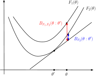
Figure 4: The duo Bregman divergence induced by two strictly convex and differentiable functions $F_{1}$ and $F_{2}$ such that $F_{1}(\theta)\geq F_{2}(\theta)$: We check graphically that $B_{F_{1},F_{2}}(\theta:\theta^{\prime})\geq B_{F_{2}}(\theta:\theta^{\prime})$ (vertical gaps).

Definition 2 (duo Bregman divergence).

Let $F_{1}(\theta)$ and $F_{2}(\theta)$ be two strictly convex functions such that $F_{1}(\theta)\geq F_{2}(\theta)$ for any $\theta\in\Theta_{12}=\mathrm{dom}(F_{1})\cap\mathrm{dom}(F_{2})$. Then the generalized Bregman divergence is defined by

$$\boxed{B_{F_{1},F_{2}}(\theta:\theta^{\prime})=F_{1}(\theta)-F_{2}(\theta^{\prime})-(\theta-\theta^{\prime})^{\top}\nabla F_{2}(\theta^{\prime})\geq 0.}$$ (10)

Example 2.

Consider $F_{1}(\theta)=\frac{a}{2}\theta^{2}$ for $a>0$. We have $\eta=a\theta$, $\theta=\frac{\eta}{a}$, and

$$F_{1}^{*}(\eta)=\frac{\eta^{2}}{a}-\frac{a}{2}\frac{\eta^{2}}{a^{2}}=\frac{\eta^{2}}{2a}.$$

Let $F_{2}(\theta)=\frac{1}{2}\theta^{2}$ so that $F_{1}(\theta)\geq F_{2}(\theta)$ for $a\geq 1$. We check that $F_{1}^{*}(\eta)=\frac{\eta^{2}}{2a}\leq F_{2}^{*}(\eta)$ when $a\geq 1$. The duo Fenchel-Young divergence is

$$Y_{F_{1},F_{2}^{*}}(\theta,\eta^{\prime})=\frac{a}{2}\theta^{2}+\frac{1}{2}{\eta^{\prime}}^{2}-\theta\eta^{\prime}\geq 0,$$

when $a\geq 1$. We can express the duo Fenchel-Young divergence in the primal coordinate systems as

$$B_{F_{1},F_{2}}(\theta,\theta)=\frac{a}{2}\theta^{2}+\frac{1}{2}{\theta^{\prime}}^{2}-\theta\theta^{\prime}.$$

When $a=1$, $F_{1}(\theta)=F_{2}(\theta)=\frac{1}{2}\theta^{2}:=F(\theta)$, and we get $B_{F}(\theta,\theta^{\prime})=\frac{1}{2}\|\theta-\theta^{\prime}\|_{2}^{2}$, half the squared Euclidean distance as expected. Figure 5 displays the graph plot of the duo Bregman divergence for several values $a$.

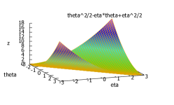
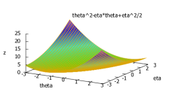
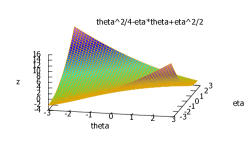
(a)	(b)	(c)

Figure 5: The duo half squared Euclidean distance $D_{a}^{2}(\theta:\theta^{\prime}):=\frac{a}{2}\theta^{2}+\frac{1}{2}{\theta^{\prime}}^{2}-\theta\theta^{\prime}$ is non-negative when $a\geq 1$: (a) half squared Euclidean distance ($a=1$), (b) $a=2$, (c) $a=\frac{1}{2}$ which shows that the divergence can be negative then since $a<1$.

Example 3.

Consider $F_{1}(\theta)=\theta^{2}$ and $F_{2}(\theta)=\theta^{4}$ on the domain $\Theta=[0,1]$. We have $F_{1}(\theta)\geq F_{2}(\theta)$ for $\theta\in\Theta$. The convex conjugate of $F_{1}(\eta)$ is $F_{1}^{*}(\eta)=\frac{1}{4}\eta^{2}$. We have

$$F_{2}^{*}(\eta)={\eta}^{\frac{4}{3}}\left(\left(\frac{1}{4}\right)^{\frac{1}{3}}-\left(\frac{1}{4}\right)^{\frac{4}{3}}\right)=\frac{3}{4^{\frac{4}{3}}}{\eta}^{\frac{4}{3}}$$

with $\eta_{2}(\theta)=4{\theta}^{3}$. Figure 6 plots the convex functions $F_{1}(\theta)$ and $F_{2}(\theta)$, and their convex conjugates $F_{1}^{*}(\eta)$ and $F_{2}^{*}(\eta)$. We observe that $F_{1}(\theta)\geq F_{2}(\theta)$ on $\theta\in[0,1]$ and that $F_{1}^{*}(\eta)\leq F_{2}^{*}(\eta)$ on $H=[0,2]$.

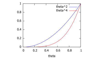
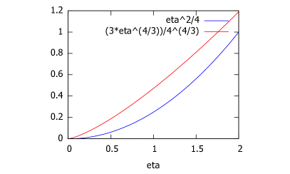
Convex functions	Conjugate functions

Figure 6: The Legendre transform reverses the dominance ordering: $F_{1}(\theta)=\theta^{2}\geq F_{2}(\theta)=\theta^{4}\Leftrightarrow F_{1}^{*}(\eta)\geq F_{2}^{*}(\eta)$ for $\theta\in[0,1]$.

We now state a property between dual duo Bregman divergences:

Property 2 (Dual duo Fenchel-Young/Bregman divergences).

We have

$$Y_{F_{1},F_{2}^{*}}(\theta:\eta^{\prime})=B_{F_{1},F_{2}}(\theta:\theta^{\prime})=B_{F_{2}^{*},F_{1}^{*}}(\eta^{\prime}:\eta)=Y_{F_{2}^{*},F_{1}}(\eta^{\prime}:\theta)$$

Proof.

From the Fenchel-Young equalities of the inequalities, we have $F_{1}(\theta)=\theta^{\top}\eta-F_{1}^{*}(\eta)$ for $\eta=\nabla F_{1}(\theta)$ and $F_{2}(\theta^{\prime})={\theta^{\prime}}^{\top}\eta^{\prime}-F_{2}^{*}(\eta^{\prime})$ with $\eta^{\prime}=\nabla F_{2}(\theta^{\prime})$. Thus we have

$$B_{F_{1},F_{2}}(\theta:\theta^{\prime}) = F_{1}(\theta)-F_{2}(\theta^{\prime})-(\theta-\theta^{\prime})^{\top}\nabla F_{2}(\theta^{\prime}),$$

$$= \theta^{\top}\eta-F_{1}^{*}(\eta)-{\theta^{\prime}}^{\top}\eta^{\prime}+F_{2}^{*}(\eta^{\prime})-(\theta-\theta^{\prime})^{\top}\eta^{\prime},$$

$$= F_{2}^{*}(\eta^{\prime})-F_{1}^{*}(\eta)-(\eta^{\prime}-\eta)^{\top}\theta,$$

$$= B_{F_{2}^{*},F_{1}^{*}}(\eta^{\prime}:\eta).$$

Recall that $F_{1}(\theta)\geq F_{2}(\theta)$ implies that $F_{1}^{*}(\eta)\leq F_{2}^{*}(\eta)$, and therefore the dual duo Bregman divergence is non-negative: $B_{F_{2}^{*},F_{1}^{*}}(\eta^{\prime}:\eta)\geq 0$. ∎

4 Kullback-Leibler divergence between a truncated density and a density of an exponential family

Let $\mathcal{E}_{1}=\{P_{\theta}\ :\ \theta\in\Theta_{1}\}$ be an exponential family of distributions all dominated by $\mu$ with Radon-Nikodym density $p_{\theta}(x)=\exp(\theta^{\top}t(x)-F_{1}(\theta)+k(x))\,\mathrm{d}\mu(x)$ defined on the support $\mathcal{X}_{1}$. Let $\mathcal{E}_{2}=\{Q_{\theta}\ :\ \theta\in\Theta_{2}\}$ be another exponential family of distributions all dominated by $\mu$ with Radon-Nikodym density $q_{\theta}(x)=\exp(\theta^{\top}t(x)-F_{2}(\theta)+k(x))\,\mathrm{d}\mu(x)$ defined on the support $\mathcal{X}_{2}$ such that $\mathcal{X}_{1}\subseteq\mathcal{X}_{2}$. Let $\tilde{p}_{\theta}(x)=\exp(\theta^{\top}t(x)+k(x))\,\mathrm{d}\mu(x)$ be the common unnormalized density so that

$$p_{\theta}(x)=\frac{\tilde{p}_{\theta}(x)}{Z_{1}(\theta)}$$

and

$$q_{\theta}(x)=\frac{\tilde{p}_{\theta}(x)}{Z_{2}(\theta)}=\frac{Z_{1}(\theta)}{Z_{2}(\theta)}\,p_{\theta}(x),$$

with $Z_{1}(\theta)=\exp(F_{1}(\theta))$ and $Z_{2}(\theta)=\exp(F_{2}(\theta))$ are the log-normalizer functions of $\mathcal{E}_{1}$ and $\mathcal{E}_{2}$, respectively.

We have

$$D_{\mathrm{KL}}[p_{\theta_{1}}:q_{\theta_{2}}] = \int_{\mathcal{X}_{1}}p_{\theta_{1}}(x)\log\frac{p_{\theta_{1}}(x)}{q_{\theta_{2}}(x)}\mathrm{d}\mu(x),$$

$$= \int_{\mathcal{X}_{1}}p_{\theta_{1}}(x)\log\frac{p_{\theta_{1}}(x)}{p_{\theta_{2}}(x)}\mathrm{d}\mu(x)+\int_{\mathcal{X}_{1}}p_{\theta_{1}}(x)\log\left(\frac{Z_{2}(\theta_{2})}{Z_{1}(\theta_{2})}\right),$$

$$= D_{\mathrm{KL}}[p_{\theta_{1}}:p_{\theta_{2}}]+\log Z_{2}(\theta_{2})-\log Z_{1}(\theta_{2}).$$

Since $D_{\mathrm{KL}}[p_{\theta_{1}}:p_{\theta_{2}}]=B_{F_{1}}(\theta_{2}:\theta_{1})$ and $\log Z_{i}(\theta)=F_{i}(\theta)$, we get

$$D_{\mathrm{KL}}[p_{\theta_{1}}:q_{\theta_{2}}] = B_{F_{1}}(\theta_{2}:\theta_{1})+F_{2}(\theta_{2})-F_{1}(\theta_{2}),$$

$$= F_{1}(\theta_{2})-F_{1}(\theta_{1})-(\theta_{2}-\theta_{1})^{\top}\nabla F_{1}(\theta_{1})+F_{2}(\theta_{2})-F_{1}(\theta_{2}),$$

$$= F_{2}(\theta_{2})-F_{1}(\theta_{1})-(\theta_{2}-\theta_{1})^{\top}\nabla F_{1}(\theta_{1})=:B_{F_{2},F_{1}}(\theta_{2}:\theta_{1}).$$

Observe that we have:

$$F_{2}(\theta)=\log\int_{\mathcal{X}_{2}}\tilde{p}_{\theta}(x)\,\mathrm{d}\mu(x)\geq\log\int_{\mathcal{X}_{1}}\tilde{p}_{\theta}(x)))\,\mathrm{d}\mu(x):=F_{1}(\theta),$$

since $\mathcal{X}_{1}\subseteq\mathcal{X}2$. Therefore $\Theta_{2}\subseteq\Theta_{1}$, and the common natural parameter space is $\Theta_{12}=\Theta_{1}\cap\Theta_{2}=\Theta_{2}$.

Notice that the reverse Kullback-Leibler divergence $D_{\mathrm{KL}}^{*}[p_{\theta_{1}}:q_{\theta_{2}}]=D_{\mathrm{KL}}[q_{\theta_{2}}:p_{\theta_{1}}]=+\infty$ since $Q_{\theta_{2}}\not\ll P_{\theta_{1}}$.

Theorem 1 (Kullback-Leibler divergence between nested exponential family densities).

Let $\mathcal{E}_{2}=\{q_{\theta_{2}}\}$ be an exponential family with support $\mathcal{X}_{2}$, and $\mathcal{E}_{1}=\{p_{\theta_{1}}\}$ a truncated exponential family of $\mathcal{E}_{2}$ with support $\mathcal{X}_{1}\subset\mathcal{X}_{2}$. Let $F_{1}$ and $F_{2}$ denote the log-normalizers of $\mathcal{E}_{1}$ and $\mathcal{E}_{2}$ and $\eta_{1}$ and $\eta_{2}$ the moment parameters corresponding to the natural parameters $\theta_{1}$ and $\theta_{2}$. Then the Kullback-Leibler divergence between a truncated density of $\mathcal{E}_{1}$ and a density of $\mathcal{E}_{2}$ is

$$D_{\mathrm{KL}}[p_{\theta_{1}}:q_{\theta_{2}}]=Y_{F_{2},F_{1}^{*}}(\theta_{2}:\eta_{1})=B_{F_{2},F_{1}}(\theta_{2}:\theta_{1})=B_{F_{1}^{*},F_{2}^{*}}(\eta_{1}:\eta_{2})=Y_{F_{1}^{*},F_{2}}(\eta_{1}:\theta_{2}).$$

For example, consider the calculation of the KLD between an exponential distribution (view as half a Laplacian distribution) and a Laplacian distribution.

Example 4.

Let $\mathcal{E}_{1}=\{p_{\lambda}(x)=\lambda\exp(-\lambda x),\lambda\in\mathbb{R}_{++},x>0\}$ and $\mathcal{E}_{2}=\{q_{\lambda}(x)=\lambda\exp(-\lambda|x|),\lambda\in\mathbb{R}_{++},x\in\mathbb{R}\}$ denote the exponential families of exponential distributions and Laplacian distributions, respectively. We have the sufficient statistic $t(x)=-|x|$ and natural parameter $\theta=\lambda$ so that $\tilde{p}_{\theta}(x)=\exp(-|x|\theta)$. The log-normalizers are $F_{1}(\theta)=-\log\theta$ and $F_{2}(\theta)=-\log\theta+\log 2$ (hence $F_{2}(\theta)\geq F_{1}(\theta)$). The moment parameter $\eta=\nabla F_{1}(\theta)=\nabla F_{2}(\theta)=-\frac{1}{\theta}=-\frac{1}{\lambda}$. Thus using the duo Bregman divergence, we have:

$$D_{\mathrm{KL}}[p_{\theta_{1}}:q_{\theta_{2}}] = B_{F_{2},F_{1}}(\theta_{2}:\theta_{1}),$$

$$= F_{2}(\theta_{2})-F_{1}(\theta_{1})-(\theta_{2}-\theta_{1})^{\top}\nabla F_{1}(\theta_{1}),$$

$$= \log 2+\log\frac{\lambda_{1}}{\lambda_{2}}+\frac{\lambda_{2}}{\lambda_{1}}-1.$$

Moreover, we can interpret that divergence using the Itakura-Saito divergence [16]:

$$D_{\mathrm{IS}}[\lambda_{1}:\lambda_{2}]:=\frac{\lambda_{1}}{\lambda_{2}}-\log\frac{\lambda_{1}}{\lambda_{2}}-1\geq 0.$$

we have

$$D_{\mathrm{KL}}[p_{\theta_{1}}:q_{\theta_{2}}]=D_{\mathrm{IS}}[\lambda_{2}:\lambda_{1}]+\log 2\geq 0.$$

We check the result using the duo Fenchel-Young divergence:

$$D_{\mathrm{KL}}[p_{\theta_{1}}:q_{\theta_{2}}]=Y_{F_{2},F_{1}^{*}}(\theta_{2}:\eta_{1}),$$

with $F_{1}^{*}(\eta)=-1+\log\left(-\frac{1}{\eta}\right)$:

$$D_{\mathrm{KL}}[p_{\theta_{1}}:q_{\theta_{2}}] = Y_{F_{2},F_{1}^{*}}(\theta_{2}:\eta_{1}),$$

$$= -\log\lambda_{2}+\log 2-1+\log\lambda_{1}+\frac{\lambda_{2}}{\lambda_{1}},$$

$$= \log\frac{\lambda_{1}}{\lambda_{2}}+\frac{\lambda_{2}}{\lambda_{1}}+\log_{2}-1.$$

Next, consider the calculation of the KLD between a half-normal distribution and a (full) normal distribution:

Example 5.

Consider $\mathcal{E}_{1}$ and $\mathcal{E}_{2}$ be the scale family of the half standard normal distributions and the scale family of the standard normal distribution, respectively. We have $\tilde{p}_{\theta}(x)=\exp\left(-\frac{x^{2}}{2\sigma^{2}}\right)$ with $Z_{1}(\theta)=\sigma\sqrt{\frac{\pi}{2}}$ and $Z_{2}(\theta)=\sigma\sqrt{2\pi}$. Let the sufficient statistic be $t(x)=-\frac{x^{2}}{2}$ so that the natural parameter is $\theta=\frac{1}{\sigma^{2}}\in\mathbb{R}_{++}$. Here, we have both $\Theta_{1}=\Theta_{2}=\mathbb{R}_{++}$. For this example, we check that $Z_{1}(\theta)=\frac{1}{2}\,Z_{2}(\theta)$. We have $F_{1}(\theta)=-\frac{1}{2}\log\theta+\frac{1}{2}\log\frac{\pi}{2}$ and $F_{2}(\theta)=-\frac{1}{2}\log\theta+\frac{1}{2}\log(2\pi)$ (with $F_{2}(\theta)\geq F_{1}(\theta)$). We have $\eta=-\frac{1}{2\theta}=-\frac{1}{2}\sigma^{2}$. The KLD between two half scale normal distributions is

$$D_{\mathrm{KL}}[p_{\theta_{1}}:p_{\theta_{2}}] = B_{F_{1}}(\theta_{2}:\theta_{1}),$$

$$= \frac{1}{2}\left(\log\frac{\sigma_{2}^{2}}{\sigma_{1}^{2}}+\frac{\sigma_{1}^{2}}{\sigma_{2}^{2}}-1\right).$$

Since $F_{1}(\theta)$ and $F_{2}(\theta)$ differ only by a constant and that the Bregman divergence is invariant under an affine term of its generator, we have

$$D_{\mathrm{KL}}[q_{\theta_{1}}:q_{\theta_{2}}] = B_{F_{2}}(\theta_{2}:\theta_{1}),$$

$$= B_{F_{1}}(\theta_{2}:\theta_{1})=\frac{1}{2}\left(\log\frac{\sigma_{2}^{2}}{\sigma_{1}^{2}}+\frac{\sigma_{1}^{2}}{\sigma_{2}^{2}}-1\right).$$

Moreover, we can interpret those Bregman divergences as half of the Itakura-Saito divergence:

$$D_{\mathrm{KL}}[p_{\theta_{1}}:p_{\theta_{2}}]=D_{\mathrm{KL}}[q_{\theta_{1}}:q_{\theta_{2}}]=B_{F_{2}}(\theta_{2}:\theta_{1})=\frac{1}{2}D_{\mathrm{IS}}[\sigma_{1}^{2}:\sigma_{2}^{2}],$$

where

$$D_{\mathrm{IS}}[\lambda_{1}:\lambda_{2}]:=\frac{\lambda_{1}}{\lambda_{2}}-\log\frac{\lambda_{1}}{\lambda_{2}}-1.$$

It follows that

$$D_{\mathrm{KL}}[p_{\theta_{1}}:q_{\theta_{2}}] = B_{F_{2},F_{1}}(\theta_{2}:\theta_{1})=F_{2}(\theta_{2})-F_{1}(\theta_{1})-(\theta_{2}-\theta_{1})^{\top}\nabla F_{1}(\theta_{1}),$$

$$= \frac{1}{2}\left(\log\frac{\sigma_{2}^{2}}{\sigma_{1}^{2}}+{\sigma_{1}^{2}}{\sigma_{2}^{2}}+\log 4-1\right).$$

Notice that $\frac{1}{2}\log 4=\log 2>0$ so that $D_{\mathrm{KL}}[p_{\theta_{1}}:q_{\theta_{2}}]\geq D_{\mathrm{KL}}[q_{\theta_{1}}:q_{\theta_{2}}]$.

Thus the Kullback-Leibler divergence between a truncated density and another density of the same exponential family amounts to calculate a duo Bregman divergence on the reverse parameter order: $D_{\mathrm{KL}}[p_{\theta_{1}}:q_{\theta_{2}}]=B_{F_{2},F_{1}}(\theta_{2}:\theta_{1})$. Let $D_{\mathrm{KL}}^{*}[p:q]:=D_{\mathrm{KL}}[q:p]$ be the reverse Kullback-Leibler divergence. Then $D_{\mathrm{KL}}^{*}[q_{\theta_{2}}:p_{\theta_{1}}]=B_{F_{2},F_{1}}(\theta_{2}:\theta_{1})$.

Notice that truncated exponential families are also exponential families but they may be non-steep [11].

The next example shows how to compute the Kullback-Leibler divergence between two truncated normal distributions:

Example 6.

Let $N_{a,b}(m,s)$ denote a truncated normal distribution with support the open interval $(a,b)$ ($a<b$) and probability density function (pdf) defined by:

$$p_{m,s}^{a,b}(x)=\frac{1}{Z_{a,b}(m,s)}\,\exp\left(-\frac{(x-m)^{2}}{2s^{2}}\right),$$

where $Z_{a,b}(m,s)$ is related to the partition function [8] expressed using the cumulative distribution function (CDF) $\Phi_{m,s}(x)$:

$$Z_{a,b}(m,s)=\sqrt{2\pi}s\,\left(\Phi_{m,s}(b)-\Phi_{m,s}(a)\right),$$

with

$$\Phi_{m,s}(x)=\frac{1}{2}\left(1+\mathrm{erf}\left(\frac{x-m}{\sqrt{2}s}\right)\right),$$

where $\mathrm{erf}(x)$ is the error function:

$$\mathrm{erf}(x):=\frac{2}{\sqrt{\pi}}\,\int_{0}^{x}e^{-t^{2}}\mathrm{d}t.$$

Thus we have $\mathrm{erf}(x)=2\,\Phi(\sqrt{2}x)-1$ where $\Phi(x)=\Phi_{0,1}(x)$.

The pdf can also be written as

$$p_{m,s}^{a,b}(x)=\frac{1}{\sigma}\frac{\phi(\frac{x-m}{s})}{\Phi(\frac{b-m}{s})-\Phi(\frac{a-m}{s})},$$

where $\phi(x)$ denotes the standard normal pdf ($\phi(x)=p_{0,1}^{-\infty,+\infty}(x)$):

$$\phi(x):=\frac{1}{\sqrt{2\pi}}\,\exp\left(-\frac{x^{2}}{2}\right),$$

and $\Phi(x)=\Phi_{0,1}(x)=\int_{-\infty}^{x}\phi(t)\,\mathrm{d}t$ is the standard normal CDF. When $a=-\infty$ and $b=+\infty$, we have $Z_{-\infty,\infty}(m,s)=\sqrt{2\pi}\,s$ since $\Phi(-\infty)=0$ and $\Phi(+\infty)=1$.

The density $p_{m,s}^{a,b}(x)$ belongs to an exponential family $\mathcal{E}_{a,b}$ with natural parameter $\theta=\left(\frac{m}{s^{2}},-\frac{1}{2s^{2}}\right)$, sufficient statistics $t(x)=(x,x^{2})$, and log-normalizer:

$$F_{a,b}(\theta)=-\frac{\theta_{1}^{2}}{4\theta_{2}}+\log Z_{a,b}(\theta)$$

The natural parameter space is $\Theta=\mathbb{R}\times\mathbb{R}_{--}$ where $\mathbb{R}_{--}$ denotes the set of negative real numbers.

The log-normalizer can be expressed using the source parameters $(m,s)$ (which are not the mean and standard deviation when the support is truncated, hence the notation $m$ and $s$):

$$F_{a,b}(m,s) = \frac{m^{2}}{2s^{2}}+\log Z_{a,b}(m,s),$$

$$= \frac{m^{2}}{2s^{2}}+\frac{1}{2}\log 2\pi s^{2}+\log\left(\Phi_{m,s}(b)-\Phi_{m,s}(a)\right).$$

We shall use the fact that the gradient of the log-normalizer of any exponential family distribution amounts to the expectation of the sufficient statistics [28]:

$$\nabla F_{a,b}(\theta)=E_{p_{m,s}^{a,b}}[t(x)]=\eta.$$

Parameter $\eta$ is called the moment or expectation parameter [28].

The mean $\mu(m,s;a,b)=E_{p_{m,s}^{a,b}}[x]=\frac{\partial}{\partial\theta_{1}}F_{a,b}(\theta)$ and the variance $\sigma^{2}(m,s;a,b)=E_{p_{m,s}^{a,b}}[x^{2}]-\mu^{2}$ (with $E_{p_{m,s}^{a,b}}[x^{2}]=\frac{\partial}{\partial\theta_{2}}F_{a,b}(\theta)$) of the truncated normal $p_{m,s}^{a,b}$ can be expressed using the following formula [18, 8] (page 25):

$$\mu(m,s;a,b) = m-s\,\frac{\phi(\beta)-\phi(\alpha)}{\Phi(\beta)-\Phi(\alpha)},$$

$$\sigma^{2}(m,s;a,b) = s^{2}\,\left(1-\frac{\beta\phi(\beta)-\alpha\phi(\alpha)}{\Phi(\beta)-\Phi(\alpha)}-\left(\frac{\phi(\beta)-\phi(\alpha)}{\Phi(\beta)-\Phi(\alpha)}\right)^{2}\right),$$

where $\alpha:=\frac{a-m}{s}$ and $\beta:=\frac{b-m}{s}$. Thus we have the following moment parameter $\eta=(\eta_{1},\eta_{2})$ with

$$\eta_{1}(m,s;a,b) = E_{p_{m,s}^{a,b}}[x]=\mu(m,s;a,b),$$ (11)

$$\eta_{2}(m,s;a,b) = E_{p_{m,s}^{a,b}}[x^{2}]=\sigma^{2}(m,s;a,b)+\mu^{2}(m,s;a,b).$$ (12)

Now consider two truncated normal distributions $p_{m_{1},s_{1}}^{a_{1},b_{1}}$ and $p_{m_{2},s_{2}}^{a_{2},b_{2}}$ with $[a_{1},b_{1}]\subseteq[a_{2},b_{2}]$ (otherwise, we have $D_{\mathrm{KL}}[p_{m_{1},s_{1}}^{a_{1},b_{1}}:p_{m_{2},s_{2}}^{a_{2},b_{2}}]=+\infty$). Then the KLD between $p_{m_{1},s_{1}}^{a_{1},b_{1}}$ and $p_{m_{2},s_{2}}^{a_{2},b_{2}}$ is equivalent to a duo Bregman divergence:

$$D_{\mathrm{KL}}[p_{m_{1},s_{1}}^{a_{1},b_{1}}:p_{m_{2},s_{2}}^{a_{2},b_{2}}] = F_{m_{2},s_{2}}(\theta_{2})-F_{m_{1},s_{1}}(\theta_{1})-(\theta_{2}-\theta_{1})^{\top}\nabla F_{m_{1},s_{1}}(\theta_{1}),$$ (13)

$$= \frac{m_{2}}{2s_{2}^{2}}-\frac{m_{1}}{2s_{1}^{2}}+\log\frac{Z_{a_{2},b_{2}}(m_{2},s_{2})}{Z_{a_{1},b_{1}}(m_{1},s_{1})}-\left(\frac{m_{2}}{s_{2}^{2}}-\frac{m_{1}}{s_{1}^{2}}\right)\eta_{1}(m_{1},s_{1};a_{1},b_{1})$$

$$-\left(\frac{1}{2s_{1}^{2}}-\frac{1}{2s_{2}^{2}}\right)\eta_{2}(m_{1},s_{1};a_{1},b_{1}).$$

Notice that $F_{m_{2},s_{2}}(\theta)\geq F_{m_{1},s_{1}}(\theta)$.

This formula is valid for (1) the KLD between two nested truncated normal distributions, or for (2) the KLD between a truncated normal distribution and a (full support) normal distribution. Notice that formula depends on the erf function used in function $\Phi$. Furthermore, when $a_{1}=a_{2}=-\infty$ and $b_{1}=b_{2}=+\infty$, we recover (3) the KLD between two univariate normal distributions since $\log\frac{Z_{a_{2},b_{2}}(m_{2},s_{2})}{Z_{a_{1},b_{1}}(m_{1},s_{1})}=\log\frac{\sigma_{2}}{\sigma_{1}}=\frac{1}{2}\log\frac{\sigma_{2}^{2}}{\sigma_{1}^{2}}$:

$$D_{\mathrm{KL}}[p_{m_{1},s_{1}}:p_{m_{2},s_{2}}]=\frac{1}{2}\,\left(\log\frac{s_{2}^{2}}{s_{1}^{2}}+\frac{\sigma_{1}^{2}}{\sigma_{2}^{2}}+\frac{(m_{2}-m_{1})^{2}}{s_{2}^{2}}-1.\right).$$

Notice that for full support normal distributions, $\mu(m,s;-\infty;+\infty)=m$ and $\sigma^{2}(m,s;-\infty;+\infty)=s^{2}$.

The entropy of a truncated normal distribution (an exponential family [24]) is $h[p_{m,s}^{a,b}]=-\int_{a}^{b}p_{m,s}^{a,b}(x)\log p_{m,s}^{a,b}\mathrm{d}x=-F^{*}(\eta)=F(\theta)-\theta^{\top}\eta$. We find that

$$h[p_{m,s}^{a,b}]=\log\left(\sqrt{2\pi e}s\,\left(\Phi(\beta)-\Phi(\alpha)\right)\right)+\frac{\alpha\phi(\alpha)-\beta\phi(\beta)}{2\left(\Phi(\beta)-\Phi(\alpha)\right)}.$$

When $(a,b)=(-\infty,\infty)$, we have $\Phi(\beta)-\Phi(\alpha)=1$ and $\alpha\phi(\alpha)-\beta\phi(\beta)=0$ since $\beta=-\alpha$, $\phi(-x)=\phi(x)$ (an even function), and $\lim_{\beta\rightarrow+\infty}\beta\phi(\beta)=0$. Thus we recover the differential entropy of a normal distribution: $h[p_{\mu,\sigma}]=\log\left(\sqrt{2\pi e}\sigma\right)$.

5 Bhattacharyya skewed divergence between nested densities of an exponential family

The Bhattacharyya $\alpha$-skewed divergence [5, 21] between two densities $p(x)$ and $q(x)$ with respect to $\mu$ is defined for a skewing scalar parameter $\alpha\in(0,1)$ as:

$$D_{\mathrm{Bhat},\alpha}[p:q]:=-\log\int_{\mathcal{X}}p(x)^{\alpha}q(x)^{1-\alpha}\,\mathrm{d}\mu(x),$$

where $\mathcal{X}$ denotes the support of the distributions. Let $I_{\alpha}[p:q]:=\int_{\mathcal{X}}p(x)^{\alpha}q(x)^{1-\alpha}\,\mathrm{d}\mu(x)$ denote the skewed affinity coefficient so that $D_{\mathrm{Bhat},\alpha}[p:q]=-\log I_{\alpha}[p:q]$. Since $I_{\alpha}[p:q]=I_{1-\alpha}[q:p]$, we have $D_{\mathrm{Bhat},\alpha}[p:q]=D_{\mathrm{Bhat},1-\alpha}[q:p]$.

Consider an exponential family $\mathcal{E}=\{p_{\theta}\}$ with log-normalizer $F(\theta)$. Then it is well-known that the $\alpha$-skewed Bhattacharyya divergence between two densities of an exponential family amounts to a skewed Jensen divergence [21] (originally called Jensen difference in [26]):

$$D_{\mathrm{Bhat},\alpha}[p_{\theta_{1}}:p_{\theta_{2}}]=J_{F,\alpha}(\theta_{1}:\theta_{2}),$$

where the skewed Jensen divergence is defined by

$$J_{F,\alpha}(\theta_{1}:\theta_{2})=\alpha F(\theta_{1})+(1-\alpha)F(\theta_{2})-F(\alpha\theta_{1}+(1-\alpha)\theta_{2}).$$

The convexity of the log-normalizer $F(\theta)$ ensures that $J_{F,\alpha}(\theta_{1}:\theta_{2})\geq 0$. The Jensen divergence can be extended to full real $\alpha$ by rescaling it by $\frac{1}{\alpha(1-\alpha)}$, see [29].

Remark 1.

The Bhattacharyya skewed divergence $D_{\mathrm{Bhat},\alpha}[p:q]$ appears naturally as the negative of the log-normalizer of the exponential family induced by the exponential arc $\{r_{\alpha}(x)\>\alpha\in(0,1)\}$ linking two densities $p$ and $q$ with $r_{\alpha}(x)\propto p(x)^{\alpha}q(x)^{1-\alpha}$. This arc is an exponential family of order $1$:

$$r_{\alpha}(x) = \exp\left(\alpha\log p(x)+(1-\alpha)\log q(x)-\log Z_{\alpha}(p:q)\right),$$

$$= \exp\left(\alpha\log\frac{p(x)}{q(x)}-F_{pq}(\alpha)\right)\,q(x).$$

The sufficient statistic is $t(x)=\frac{p(x)}{q(x)}$, the natural parameter $\alpha\in(0,1)$ and the log-normalizer $F_{pq}(\alpha)=\log Z_{\alpha}(p:q)=\log\int p(x)^{\alpha}q(x)^{1-\alpha}\mathrm{d}\mu(x)=-D_{\mathrm{Bhat},\alpha}[p:q]$. This shows that $D_{\mathrm{Bhat},\alpha}[p:q]$ is concave with respect to $\alpha$ since log-normalizers $F_{pq}(\alpha)$ are always convex. Grünwald called those exponential families: The likelihood ratio exponential families [14].

Now, consider calculating $D_{\mathrm{Bhat},\alpha}[p_{\theta_{1}}:q_{\theta_{2}}]$ where $p_{\theta_{1}}\in\mathcal{E}_{1}$ with $\mathcal{E}_{1}$ a nested exponential family of $\mathcal{E}_{2}$ and $q_{\theta_{2}}\in\mathcal{E}_{2}=\{q_{\theta}\}$. We have $q_{\theta}(x)=\frac{Z_{1}(\theta)}{Z_{2}(\theta)}p_{\theta}(x)$, where $Z_{1}(\theta)$ and $Z_{2}(\theta)$ are the partition functions of $\mathcal{E}_{1}$ and $\mathcal{E}_{2}$, respectively. Thus we have

$$I_{\alpha}[p_{\theta_{1}}:q_{\theta_{2}}]=\left(\frac{Z_{1}(\theta_{2})}{Z_{2}(\theta_{2})}\right)^{1-\alpha}\,I_{\alpha}[p_{\theta_{1}}:p_{\theta_{2}}],$$

and the $\alpha$-skewed Bhattacharyya divergence is

$$D_{\mathrm{Bhat},\alpha}[p_{\theta_{1}}:q_{\theta_{2}}]=D_{\mathrm{Bhat},\alpha}[p_{\theta_{1}}:p_{\theta_{2}}]-(1-\alpha)(F_{1}(\theta_{2})-F_{2}(\theta_{2})).$$

Therefore we get

$$D_{\mathrm{Bhat},\alpha}[p_{\theta_{1}}:q_{\theta_{2}}] = J_{F_{1},\alpha}(\theta_{1}:\theta_{2})-(1-\alpha)(F_{1}(\theta_{2})-F_{2}(\theta_{2})),$$

$$= \alpha F_{1}(\theta_{1})+(1-\alpha)F_{2}(\theta_{2})-F_{1}(\alpha\theta_{1}+(1-\alpha)\theta_{2}),$$

$$=: J_{F_{1},F_{2},\alpha}(\theta_{1}:\theta_{2}).$$

We call $J_{F_{1},F_{2},\alpha}(\theta_{1}:\theta_{2})$ the duo Jensen divergence. Since $F_{2}(\theta)\geq F_{1}(\theta)$, we check that

$$J_{F_{1},F_{2},\alpha}(\theta_{1}:\theta_{2})\geq J_{F_{1},\alpha}(\theta_{1}:\theta_{2})\geq 0.$$

Figure 7 illustrates graphically the duo Jensen divergence $J_{F_{1},F_{2},\alpha}(\theta_{1}:\theta_{2})$.

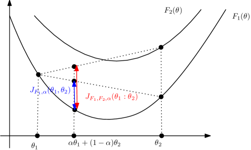
Figure 7: The duo Jensen divergence $J_{F_{1},F_{2},\alpha}(\theta_{1}:\theta_{2})$ is greater than the Jensen divergence $J_{F_{1},\alpha}(\theta_{1}:\theta_{2})$ for $F_{2}(\theta)\geq F_{1}(\theta)$.

Theorem 2.

The $\alpha$-skewed Bhattacharyya divergence for $\alpha\in(0,1)$ between a truncated density of $\mathcal{E}_{1}$ with log-normalizer $F_{1}(\theta)$ and another density of an exponential family $\mathcal{E}_{2}$ with log-normalizer $F_{2}(\theta)$ amounts to a duo Jensen divergence:

$$D_{\mathrm{Bhat},\alpha}[p_{\theta_{1}}:q_{\theta_{2}}]=J_{F_{1},F_{2},\alpha}(\theta_{1}:\theta_{2}),$$

where $J_{F_{1},F_{2},\alpha}(\theta_{1}:\theta_{2})$ is the duo skewed Jensen divergence induced by two strictly convex functions $F_{1}(\theta)$ and $F_{2}(\theta)$ such that $F_{2}(\theta)\geq F_{1}(\theta)$:

$$J_{F_{1},F_{2},\alpha}(\theta_{1}:\theta_{2})=\alpha F_{1}(\theta_{1})+(1-\alpha)F_{2}(\theta_{2})-F_{1}(\alpha\theta_{1}+(1-\alpha)\theta_{2}).$$

In [21], it is reported that

$$D_{\mathrm{KL}}[p_{\theta_{1}}:p_{\theta_{2}}] = B_{F}(\theta_{2}:\theta_{1}),$$

$$= \lim_{\alpha\rightarrow 0}\frac{1}{\alpha}J_{F,\alpha}(\theta_{2}:\theta_{1})=\lim_{\alpha\rightarrow 0}\frac{1}{\alpha}J_{F,1-\alpha}(\theta_{1}:\theta_{2}),$$

$$= \lim_{\alpha\rightarrow 0}\frac{1}{\alpha}D_{\mathrm{Bhat},\alpha}[p_{\theta_{2}}:p_{\theta_{1}}]=\lim_{\alpha\rightarrow 0}\frac{1}{\alpha}D_{\mathrm{Bhat},1-\alpha}[p_{\theta_{1}}:p_{\theta_{2}}].$$

Indeed, using the first order Taylor expansion of

$$F(\theta_{1}+\alpha(\theta_{2}-\theta_{1}))=F(\theta_{1})+\alpha(\theta_{2}-\theta_{1})^{\top}\nabla F(\theta_{1})$$

when $\alpha\rightarrow 0$, we check that we have

$$\frac{1}{\alpha}J_{F,\alpha}(\theta_{2}:\theta_{1}) \approx_{\alpha\rightarrow 0} \frac{F(\theta_{1})+\alpha(F(\theta_{2})-F(\theta_{1}))-F(\theta_{1}+\alpha(\theta_{2}-\theta_{1}))}{\alpha},$$

$$= B_{F}(\theta_{2}:\theta_{1}).$$

Moreover, we have

$$\lim_{\alpha\rightarrow 0}\frac{1}{\alpha}D_{\mathrm{Bhat},1-\alpha}[p:q]=D_{\mathrm{KL}}[p:q].$$

Similarly, we can prove that

$$\lim_{\alpha\rightarrow 1}\frac{1}{1-\alpha}J_{F_{1},F_{2},\alpha}(\theta_{1}:\theta_{2})=B_{F_{2},F_{1}}(\theta_{2}:\theta_{1}),$$

which can be reinterpreted as

$$\lim_{\alpha\rightarrow 1}\frac{1}{1-\alpha}D_{\mathrm{Bhat},\alpha}[p_{\theta_{1}}:q_{\theta_{2}}]=D_{\mathrm{KL}}[p_{\theta_{1}}:q_{\theta_{2}}].$$

6 Sided duo Bregman centroids

A centroid of a finite set of $n$ parameters $\{\theta_{1},\ldots,\theta_{n}\}$ with respect to a divergence $D(\cdot:\cdot)$ is defined by the following minimization problem:

$$\min_{\theta}\frac{1}{n}\sum_{i=1}^{n}D(\theta:\theta_{i}).$$ (14)

When $D(\theta:\theta^{\prime})=\|\theta-\theta^{\prime}\|^{2}$m the centroid corresponds to the center of mass $\bar{\theta}=\frac{1}{n}\sum_{i=1}^{n}\theta_{i}$.

Since the divergence $D(\cdot:\cdot)$ may be asymmetric, we may also consider the centroid defined with respect to the dual divergence $D^{*}(\theta:\theta^{\prime})=D(\theta^{\prime}:\theta)$ (also called the reverse divergence or backward divergence):

$$\min_{\theta}\frac{1}{n}\sum_{i=1}^{n}D^{*}(\theta:\theta_{i})=\min_{\theta}\frac{1}{n}\sum_{i=1}^{n}D(\theta_{i}:\theta).$$ (15)

We shall call the minimizer(s) of Eq. 14 the left-sided centroid(s) and the minimizer(s) of Eq. 15 the right-sided centroid(s).

Now, consider the duo Bregman left-sided centroid defined by the following minimization problem:

$$\min_{\theta^{L}}\frac{1}{n}\sum_{i=1}^{n}B_{F_{1},F_{2}}(\theta^{L}:\theta_{i}).$$ (16)

Using the equivalent duo Fenchel-Young divergence of Eq. 9, the minimization of Eq. 16 amounts equivalently to

$$\min_{\theta^{L}}L(\theta^{L}):=\sum_{i=1}^{n}Y_{F_{1},F_{2}^{*}}(\theta^{L}:\eta_{i})=\sum_{i=1}^{n}F_{1}(\theta^{L})+F_{2}^{*}(\eta_{i})-{\theta^{L}}^{\top}\eta_{i},$$

where $\eta_{i}=\nabla F_{2}(\theta_{i})$. Setting the gradient of $L(\theta^{L})$ to zero, we find that $\nabla F_{1}(\theta^{L})=\frac{1}{n}\sum_{i=1}^{n}\eta_{i}:=\bar{\eta}$. Thus we have

$$\theta^{L}=(\nabla F_{1})^{-1}\left(\frac{1}{n}\sum_{i=1}^{n}\nabla F_{2}(\theta_{i})\right).$$ (17)

When $F_{2}=F_{1}=F$ and $F$ is coordinate-wise separable, Eq. 17 is a multivariate quasi-arithmetic mean [21].

Next, consider the duo Bregman right-sided centroid:

$$\min_{\theta^{R}}\sum_{i=1}^{n}B_{F_{1},F_{2}}(\theta_{i}:\theta^{R}).$$

Using the equivalent duo Fenchel-Young divergence, the minimization amounts equivalently to

$$\min_{\theta^{R}}R(\theta^{R}):=\sum_{i=1}^{n}Y_{F_{1},F_{2}^{*}}(\theta_{i}:\eta^{R})=\sum_{i=1}^{n}F_{1}(\theta_{i})+F_{2}^{*}(\eta^{R})-{\theta_{i}}^{\top}\eta^{R},$$

where $\eta^{R}=\nabla F_{2}(\theta^{R})$. Setting the gradient of $R(\theta^{R})$ to zero, we find that $\nabla F_{2}^{*}(\eta^{R})=\frac{1}{n}\sum_{i=1}^{n}\theta_{i}$. That is, we get

$$\eta^{R}=(\nabla F_{2}^{*})^{-1}\left(\frac{1}{n}\sum_{i=1}^{n}\theta_{i}\right)=\nabla F_{2}(\theta^{R}).$$

Since $(\nabla F_{2})^{-1}=(\nabla F_{2}^{*})$, we get

$$\theta^{R}=\frac{1}{n}\sum_{i=1}^{n}\theta_{i}:=\bar{\theta}.$$ (18)

Thus the duo Bregman right-sided centroid is always the center of mass. This generalizes the result of Banerjee et al. [4] (Proposition 1).

Notice that the symmetrized duo Bregman divergence is

$$S_{F_{1},F_{2}}(\theta_{1},\theta_{2}) = B_{F_{1},F_{2}}(\theta_{1}:\theta_{2})+B_{F_{1},F_{2}}(\theta_{2}:\theta_{1}),$$

$$= (\theta_{1}-\theta_{2})^{\top}(\nabla F_{2}(\theta_{1})-\nabla F_{2}(\theta_{2}))+(F_{1}(\theta_{1})-F_{2}(\theta_{1})+F_{1}(\theta_{2})-F_{2}(\theta_{2})).$$

When $F_{1}=F_{2}=F$, we recover the ordinary symmetrized Bregman divergence [23]:

$$S_{F}(\theta_{1},\theta_{2})=S_{F,F}(\theta_{1},\theta_{2})=(\theta_{1}-\theta_{2})^{\top}(\nabla F(\theta_{1})-\nabla F(\theta_{2})).$$

7 Concluding remarks

We considered the Kullback-Leibler divergence between two parametric densities $p_{\theta}\in\mathcal{E}_{1}$ and $q_{\theta^{\prime}}\in\mathcal{E}_{2}$ belonging to nested exponential families $\mathcal{E}_{1}$ and $\mathcal{E}_{2}$, and we showed that their KLD is equivalent to a duo Bregman divergence on swapped parameter order (Theorem 1). This result generalizes the study of Azoury and Warmuth [3]. The duo Bregman divergence can be rewritten as a duo Fenchel-Young divergence using mixed natural/moment parameterizations of the exponential family densities (Definition 1). This second result generalizes the approach taken in information geometry [2]. We showed how to calculate the Kullback-Leibler divergence between two truncated normal distributions as a duo Bregman divergence. More generally, we proved that the skewed Bhattacharyya distance between two parametric nested exponential family densities amount to a duo Jensen divergence (Theorem 2). We show asymptotically that scaled duo Jensen divergences tend to duo Bregman divergences generalizing a result of [29, 21]. This study of duo divergences induced by pair of generators was motivated by the formula obtained for the Kullback-Leibler divergence between two densities of two different exponential families originally reported in [20] (Eq. 5). We called those duo divergences although they are pseudo-divergences since those divergences are always strictly greater than zero when the first generators are strictly majorizing the second generators.

It is interesting to find applications of the duo Fenchel-Young, Bregman, and Jensen divergences beyond the scope of calculating statistical distances between nested exponential family densities. Let us point out that nested exponential families have been seldom considered in the literature (see [25] for a recent work). Notice that in [22], the authors exhibit a relationship between densities with nested supports and quasi-convex Bregman divergences. Recently, Khan and Swaroop [13] used this duo Fenchel-Young divergence in machine learning for knowledge-adaptation priors in the so-called change regularizer task.

References

- [1] Sreangsu Acharyya. Learning to rank in supervised and unsupervised settings using convexity and monotonicity. PhD thesis, The University of Texas at Austin, USA, 2013.
- [2] Shun-ichi Amari. Differential-geometrical methods in statistics. Lecture Notes on Statistics, 28:1, 1985.
- [3] Katy S Azoury and Manfred K Warmuth. Relative loss bounds for on-line density estimation with the exponential family of distributions. Machine Learning, 43(3):211–246, 2001.
- [4] Arindam Banerjee, Srujana Merugu, Inderjit S Dhillon, Joydeep Ghosh, and John Lafferty. Clustering with Bregman divergences. Journal of machine learning research, 6(10), 2005.
- [5] Anil Bhattacharyya. On a measure of divergence between two statistical populations defined by their probability distributions. Bull. Calcutta Math. Soc., 35:99–109, 1943.
- [6] Mathieu Blondel, André FT Martins, and Vlad Niculae. Learning with fenchel-young losses. J. Mach. Learn. Res., 21(35):1–69, 2020.
- [7] Lev M Bregman. The relaxation method of finding the common point of convex sets and its application to the solution of problems in convex programming. USSR computational mathematics and mathematical physics, 7(3):200–217, 1967.
- [8] John Burkardt. The truncated normal distribution. Technical report, Department of Scientific Computing Website, Florida State University, 2014.
- [9] Thomas M Cover. Elements of information theory. John Wiley & Sons, 1999.
- [10] Imre Csiszár. Eine informationstheoretische Ungleichung und ihre Anwendung auf Beweis der Ergodizitaet von Markoffschen Ketten. Magyer Tud. Akad. Mat. Kutato Int. Koezl., 8:85–108, 1964.
- [11] Joan Del Castillo. The singly truncated normal distribution: a non-steep exponential family. Annals of the Institute of Statistical Mathematics, 46(1):57–66, 1994.
- [12] Bradley Efron and Trevor Hastie. Computer Age Statistical Inference: Algorithms, Evidence, and Data Science, volume 6. Cambridge University Press, 2021.
- [13] Mohammad Emtiyaz Khan and Siddharth Swaroop. Knowledge-adaptation priors. arXiv e-prints, pages arXiv–2106, 2021.
- [14] Peter D Grünwald. The minimum description length principle. MIT press, 2007.
- [15] Yoshimitsu Hiejima. Interpretation of the quasi-likelihood via the tilted exponential family. Journal of the Japan Statistical Society, 27(2):157–164, 1997.
- [16] Fumitada Itakura and S. Saito. Analysis synthesis telephony based on the maximum likelihood method. In The 6th international congress on acoustics, pages 280–292, 1968.
- [17] Harold Jeffreys. The theory of probability. OUP Oxford, 1998.
- [18] Johnson Kotz and Balakrishan. Continuous Univariate Distributions, Volumes I and II. John Wiley and Sons, 1994.
- [19] Frank Nielsen. An elementary introduction to information geometry. Entropy, 22(10):1100, 2020.
- [20] Frank Nielsen. On a variational definition for the Jensen-Shannon symmetrization of distances based on the information radius. Entropy, 23(4):464, 2021.
- [21] Frank Nielsen and Sylvain Boltz. The Burbea-Rao and Bhattacharyya centroids. IEEE Transactions on Information Theory, 57(8):5455–5466, 2011.
- [22] Frank Nielsen and Gaëtan Hadjeres. Quasiconvex Jensen Divergences and Quasiconvex Bregman Divergences. In Workshop on Joint Structures and Common Foundations of Statistical Physics, Information Geometry and Inference for Learning, pages 196–218. Springer, 2020.
- [23] Frank Nielsen and Richard Nock. Sided and symmetrized Bregman centroids. IEEE transactions on Information Theory, 55(6):2882–2904, 2009.
- [24] Frank Nielsen and Richard Nock. Entropies and cross-entropies of exponential families. In 2010 IEEE International Conference on Image Processing, pages 3621–3624. IEEE, 2010.
- [25] Zachary M Pisano, Daniel Q Naiman, and Carey E Priebe. Occam factor for gaussian models with unknown variance structure. arXiv preprint arXiv:2105.01566, 2021.
- [26] C Radhakrishna Rao. Diversity and dissimilarity coefficients: a unified approach. Theoretical population biology, 21(1):24–43, 1982.
- [27] Ralph Tyrell Rockafellar. Convex analysis. Princeton university press, 2015.
- [28] Rolf Sundberg. Statistical modelling by exponential families, volume 12. Cambridge University Press, 2019.
- [29] Jun Zhang. Divergence function, duality, and convex analysis. Neural computation, 16(1):159–195, 2004.