Risk Parity Portfolios with Skewness Risk:
An Application to Factor Investing and Alternative Risk Premia

Abstract

This article develops a model that takes into account skewness risk in risk parity portfolios. In this framework, asset returns are viewed as stochastic processes with jumps or random variables generated by a Gaussian mixture distribution. This dual representation allows us to show that skewness and jump risks are equivalent. As the mixture representation is simple, we obtain analytical formulas for computing asset risk contributions of a given portfolio. Therefore, we define risk budgeting portfolios and derive existence and uniqueness conditions. We then apply our model to the equity/bond/volatility asset mix policy. When assets exhibit jump risks like the short volatility strategy, we show that skewness-based risk parity portfolios produce better allocation than volatility-based risk parity portfolios. Finally, we illustrate how this model is suitable to manage the skewness risk of long-only equity factor portfolios and to allocate between alternative risk premia.

Keywords: Risk parity, equal risk contribution, expected shortfall, skewness, jump diffusion, Gaussian mixture model, EM algorithm, filtering theory, factor investing, alternative risk premia, short volatility strategy, diversification, skewness hedging, CTA strategy.

JEL classification: C50, C60, G11.

1 Introduction

Over the last few years, three concepts have rapidly emerged in asset management and definitively changed allocation policies of large institutional investors and pension funds around the world. These three concepts are risk parity, factor investing and alternative risk premia. They constitute the key components of risk-based investing. Risk parity is an asset allocation model, which focuses on risk diversification (Roncalli, 2013). The primary idea of factor investing is to capture risk factors, which are rewarded in the universe of equities (Ang, 2014), whereas the concept of alternative risk premia is an extension of the factor investing approach, and concerns all the asset classes (Hamdan et al., 2016). These three methods share the same philosophy. For institutional investors, the main issue is the diversification level of their allocation, that is the exposure to systematic risk factors, because idiosyncratic risks and specific bets generally disappear in large portfolios. This explains that most of factor investing portfolios and alternative risk premia portfolios are managed with a risk parity approach.

However, risk parity portfolios are generally designed to manage a long-only portfolio of traditional assets (equities and bonds). For instance, the ERC portfolio of Maillard et al. (2010) consists in allocating the same amount of risk across the assets of the portfolio. The simplicity and robustness of this portfolio have attracted many professionals. Nevertheless, one may think that it is not adapted when assets present a high jump risk. In this case, the volatility is certainly not the best metric to assess the risk of the asset. A typical example is the volatility carry risk premium, which has a very low volatility but a high skewness. Other examples are the value strategy or the long/short winners-minus-losers strategy in equities.

Portfolio allocation with skewness is an extensive field of research in finance (Kraus and Litzenberger, 1976; Harvey and Siddique, 2000; Patton, 2004; Jurczenko and Maillet, 2006; Jondeau and Rockinger, 2006; Martellini and Ziemann, 2010; Xiong and Idzorek, 2011). Most of these studies are based on the maximization of a utility function that takes into account high-order moments. Whereas these approaches are appealing from a theoretical point of view, they are not actually implemented by professionals because of their complexity and lack of robustness. Another approach consists in using the Cornish-Fisher value-at-risk. Again, this approach is not used in practice because it requires the computation of co-skewness statistics, which are difficult to estimate.

In this paper, we propose an approach as an extension of the original framework of risk parity portfolios. By noting that skewness risk is related to jump risk, we consider a regime-switching model with two states: a normal state and a state where the jumps occur. It follows that asset returns follow a Gaussian mixture model, which is easy to manipulate. Our model is related to the econometric literature on Markov switching models (Hamilton, 1989), without the ambitious nature of forecasting. The primary objective of the model is to measure the total risk of a portfolio, including both volatility and skewness risks. For that, we use the expected shortfall, a coherent and convex risk measure (thus) satisfying the Euler decomposition. We can then calculate the risk contribution of assets and define risk budgeting portfolios. We apply this framework to the equity/bond asset mix policy when we introduce a short volatility strategy. We then compare the results with those obtained with a traditional risk parity model. In particular, we illustrate the skewness aggregation dilemma found by Hamdan et al. (2016) and discuss whether the skewness risk can be hedged like the volatility risk.

This article is organized as follows. In section two, we describe the skewness model of asset returns, and analyze the relationship between jump and skewness risks. In section three, we provide analytical formulas of the expected shortfall and the corresponding risk contributions. We also define risk budgeting portfolios and study the existence/uniqueness problem. The application to the equity/bond/volatility asset mix policy is presented in section four. Section five deals with the allocation of risk factors and alternative risk premia. Finally, section six offers our concluding remarks.

2 A skewness model of asset returns

In this section, we develop a simple model for modeling skewness. We consider a standard Lévy process and approximate its density by a mixture of two Gaussian distributions. The mixture representation presents some appealing properties for computational purposes, whereas the jump-diffusion representation helps in understanding the dynamics of the model. Moreover, this framework highlights the relationship between skewness risk and jump risk.

2.1 A model of asset returns

2.1.1 The jump-diffusion representation

We consider $n$ risky assets represented by the vector of prices $S_{t}=\left(S_{1,t},\ldots,S_{n,t}\right)$. We note $B_{t}$ the price of the risk-free asset. We assume that asset prices follow a diffusion, which is governed by a standard Lévy process:

$$\left\{\begin{array}[]{l}\mathrm{d}B_{t}=rB_{t}\,\mathrm{d}t\\ \mathrm{d}S_{t}=\mathop{\rm diag}\left(S_{t}\right)\,\mathrm{d}L_{t}\\ \mathrm{d}L_{t}=\mu\,\mathrm{d}t+\Sigma^{1/2}\,\mathrm{d}W_{t}+\mathrm{d}Z_{t}\end{array}\right.$$

where $r$ is the interest rate, $\mu$ and $\Sigma$ are the vector of expected returns and the covariance matrix, $W_{t}$ is a $n$-dimensional standard Brownian motion and $Z_{t}$ is a pure $n$-dimensional jump process. We also assume that the components of $W_{t}$ and $Z_{t}$ are mutually independent.

In order to keep the model simple, the jump process $Z_{t}$ is set to a compound Poisson process with a finite number of jumps:

$$Z_{t}=\sum_{i=1}^{N_{t}}Z_{i}$$

where $N_{t}$ is a scalar Poisson process with constant intensity parameter $\lambda>0$, and $Z_{1},\ldots,Z_{N_{t}}$ are vectors of i.i.d. random jump amplitudes with law $\nu\left(\mathrm{d}z\right)$. Using standard assumptions, we have $\nu\left(\mathrm{d}z\right)=\lambda f\left(z\right)\mathrm{d}z$ where $f\left(z\right)$ is the probability density function of the multivariate Gaussian distribution $\mathcal{N}\left(\tilde{\mu},\tilde{\Sigma}\right)$, $\tilde{\mu}$ is the expected value of jump amplitudes and $\tilde{\Sigma}$ is the associated covariance matrix. In Appendix A.1, we show that the characteristic function of asset returns $R_{t}=\left(R_{1,t},\ldots,R_{n,t}\right)$ for the holding period $\mathrm{d}t$ may be approximated with the following expression:

$$\mathbb{E}\left[e^{-iu.R_{t}}\right]\approx\left(1-\lambda\,\mathrm{d}t\right)\cdot e^{\left(iu^{\top}\mu-\frac{1}{2}u^{\top}\Sigma u\right)\,\mathrm{d}t}+\left(\lambda\,\mathrm{d}t\right)\cdot e^{iu^{\top}\left(\mu\,\mathrm{d}t+\tilde{\mu}\right)-\frac{1}{2}u^{\top}\left(\Sigma\,\mathrm{d}t+\tilde{\Sigma}\right)u}$$ (1)

2.1.2 The Gaussian mixture representation

For the sake of simplicity, we make the following assumptions: jumps occur simultaneously for all assets; portfolio’s rebalancing is done at frequency $\mathrm{d}t$; between two rebalancing dates, the assets can jump with probability $\lambda\,\mathrm{d}t$. Let $R_{t}=\left(R_{1,t},\ldots,R_{n,t}\right)$ be the asset returns for the holding period $\mathrm{d}t$. Using the previous assumptions, we consider a Gaussian mixture model with two regimes to define $R_{t}$:

• The continuous component, which has probability $\left(1-\lambda\,\mathrm{d}t\right)$ to occur, is driven by the Gaussian distribution $\mathcal{N}\left(\mu\,\mathrm{d}t,\Sigma\,\mathrm{d}t\right)$;

• The jump component, which has probability $\lambda\,\mathrm{d}t$ to occur, is driven by the Gaussian distribution $\mathcal{N}\left(\tilde{\mu},\tilde{\Sigma}\right)$.

Therefore, asset returns have the following multivariate density function:

$$f\left(y\right) = \frac{1-\lambda\,\mathrm{d}t}{\left(2\pi\right)^{n/2}\left|\Sigma\,\mathrm{d}t\right|^{1/2}}\exp\left(-\frac{1}{2\,}\left(y-\mu\,\mathrm{d}t\right)^{\top}\left(\Sigma\,\mathrm{d}t\right)^{-1}\left(y-\mu\,\mathrm{d}t\right)\right)+$$

$$\frac{\lambda\,\mathrm{d}t}{\left(2\pi\right)^{n/2}\left|\Sigma\,\mathrm{d}t+\tilde{\Sigma}\right|^{1/2}}\exp\left(-\frac{1}{2}\left(y-\left(\mu\,\mathrm{d}t+\tilde{\mu}\right)\right)^{\top}\left(\Sigma\,\mathrm{d}t+\tilde{\Sigma}\right)^{-1}\left(y-\left(\mu\,\mathrm{d}t+\tilde{\mu}\right)\right)\right)$$

It follows that the characteristic function of $R_{t}$ is equal to:

$$\mathbb{E}\left[e^{-iu.R_{t}}\right]=\left(1-\lambda\,\mathrm{d}t\right)\cdot e^{\left(iu^{\top}\mu-\frac{1}{2}u^{\top}\Sigma u\right)\,\mathrm{d}t}+\left(\lambda\,\mathrm{d}t\right)\cdot e^{iu^{\top}\left(\mu\,\mathrm{d}t+\tilde{\mu}\right)-\frac{1}{2}u^{\top}\left(\Sigma\,\mathrm{d}t+\tilde{\Sigma}\right)u}$$ (2)

We notice that the characteristic functions (1) and (2) coincide. This justifies the use of a Gaussian mixture distribution for modeling asset returns.

Remark 1

Without loss of generality, we set $\mathrm{d}t$ equal to one in the sequel. This simplifies the notations without changing the results. If one prefers to consider another holding period, it suffices to scale the parameters $\mu$, $\Sigma$ and $\lambda$ by a factor $\mathrm{d}t$.

2.2 Distribution function of the portfolio’s return

Let $x=\left(x_{1},\ldots,x_{n}\right)$ be the vector of weights in the portfolio. We assume that the portfolio is fully invested meaning that $\sum_{i=1}^{n}x_{i}=1$. We note $V_{t}$ the value of the portfolio $x$ at time $t$. Let $n_{i}=x_{i}V_{t}/S_{i,t}$ the number of shares invested in asset $i$. We have:

$$\mathrm{d}V_{t} =\sum_{i=1}^{n}n_{i}\,\mathrm{d}S_{i,t}$$

$$=V_{t}x^{\top}\left(\mathop{\rm diag}S_{t}\right)^{-1}\,\mathrm{d}S_{t}$$

$$=V_{t}x^{\top}\,\mathrm{d}L_{t}$$

It follows that:

$$\frac{\mathrm{d}V_{t}}{V_{t}}=x^{\top}\,\mathrm{d}L_{t}$$

We deduce that the return of the portfolio $R\left(x\right)=\sum_{i=1}^{n}x_{i}R_{i}=x^{\top}R$ is then a mixture of two normal random variables:

$$R\left(x\right)=Y=B_{1}\cdot Y_{1}+B_{2}\cdot Y_{2}$$

where $B_{1}$ and $B_{2}=1-B_{1}$ are Bernoulli random variables with probability $\pi_{1}=1-\lambda$ and $\pi_{2}=\lambda$. The first regime corresponds to the normal case: $Y_{1}\sim\mathcal{N}\left(\mu_{1}\left(x\right),\sigma_{1}^{2}\left(x\right)\right)$ where $\mu_{1}\left(x\right)=x^{\top}\mu$ and $\sigma_{1}^{2}\left(x\right)=x^{\top}\Sigma x$. The second regime incorporates the jumps: $Y_{2}\sim\mathcal{N}\left(\mu_{2}\left(x\right),\sigma_{2}^{2}\left(x\right)\right)$ where $\mu_{2}\left(x\right)=x^{\top}\left(\mu+\tilde{\mu}\right)$ and $\sigma_{2}^{2}\left(x\right)=x^{\top}\left(\Sigma+\tilde{\Sigma}\right)x$. It follows that the portfolio’s return $R\left(x\right)$ has the following density function:

$$f\left(y\right) = \pi_{1}f_{1}\left(y\right)+\pi_{2}f_{2}\left(y\right)$$ (3)

$$= \left(1-\lambda\right)\frac{1}{\sigma_{1}\left(x\right)}\phi\left(\frac{y-\mu_{1}\left(x\right)}{\sigma_{1}\left(x\right)}\right)+\lambda\frac{1}{\sigma_{2}\left(x\right)}\phi\left(\frac{y-\mu_{2}\left(x\right)}{\sigma_{2}\left(x\right)}\right)$$

We consider a universe of two assets with the following characteristics: $\mu_{1}=5\%$, $\sigma_{1}=10\%$, $\tilde{\mu}_{1}=-20\%$, $\tilde{\sigma}_{1}=5\%$, $\mu_{2}=10\%$, $\sigma_{2}=20\%$, $\tilde{\mu}_{2}=-40\%$ and $\tilde{\sigma}_{2}=5\%$. The cross-correlations are set to $\rho=50\%$ and $\tilde{\rho}=60\%$. When the jump frequency $\lambda$ is equal to $20\%$, the probability density function of asset returns and portfolio’s returns is given in Figure 1. The shape of the distribution function depends highly on the parameter $\lambda$. Indeed, if this parameter is equal to $0$ or $1$, the portfolio’s return is Gaussian. For $\lambda\in\left]0,1\right[$, the distribution function exhibits skewness and kurtosis as shown in Figure 2.

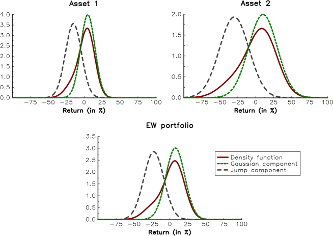
Figure 1: Probability density function of $R\left(x\right)$ when $\lambda=0.20$

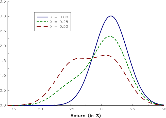
Figure 2: Probability density function of $R\left(x\right)$ for several values of $\lambda$

2.3 Relationship between jump risk and skewness risk

Using Equation (16) found in Appendix A.2, we deduce the skewness of the portfolio’s return $R\left(x\right)$ is equal to:

$$\gamma_{1}=\frac{\left(\lambda-\lambda^{2}\right)\left(\left(1-2\lambda\right)\left(x^{\top}\tilde{\mu}\right)^{3}+3\left(x^{\top}\tilde{\mu}\right)\left(x^{\top}\tilde{\Sigma}x\right)\right)}{\left(x^{\top}\Sigma x+\lambda x^{\top}\tilde{\Sigma}x+\left(\lambda-\lambda^{2}\right)\left(x^{\top}\tilde{\mu}\right)^{2}\right)^{\nicefrac{{3}}{{2}}}}$$

It follows that the model exhibits skewness, except in some limit cases. Indeed, we have:

$$\gamma_{1}=0\Leftrightarrow x^{\top}\tilde{\mu}=0\text{ or }\lambda=0\text{ or }\lambda=1$$

In the other cases, $\gamma_{1}$ may be positive or negative depending on the value of the parameters:

$$\mathop{\rm sgn}\gamma_{1}=\mathop{\rm sgn}\left(1-2\lambda\right)\left(x^{\top}\tilde{\mu}\right)^{3}+3\left(x^{\top}\tilde{\mu}\right)\left(x^{\top}\tilde{\Sigma}x\right)$$

If the expected value $x^{\top}\tilde{\mu}$ of the portfolio’s jump is positive, the skewness is then positive. If $x^{\top}\tilde{\mu}<0$, the skewness is generally negative, except if the frequency $\lambda$ is high and the variance $x^{\top}\tilde{\Sigma}x$ of the portfolio’s jump is low.

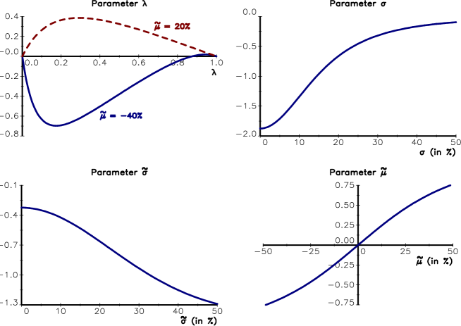
Figure 3: Skewness coefficient of the portfolio’s return $R\left(x\right)$

Let us consider a portfolio with only one asset. The parameters are equal to $\sigma=20\%$, $\tilde{\mu}=-40\%$, $\tilde{\sigma}=20\%$ and $\lambda=25\%$. In this case, we obtain $\gamma_{1}=-0.663$. In Figure 3, we show the evolution of the skewness coefficient with respect to a given parameter while the other parameters remain constant. Skewness coefficient increases with the normal volatility (top-right panel). That’s because all else being equal if the normal volatility increases, jumps get more and more indistinct from normal movements of returns. We observe that the jump’s volatility generally increases the magnitude of the skewness (bottom-left panel). The impact of the frequency $\lambda$ is more difficult to analyze, but we generally obtain a bell curve or an inverted bell curve (top-left panel).

These results are in line with those found by Hamdan et al. (2016) on the skewness risk of alternative risk premia. These authors observed that the skewness is maximum in absolute value when the portfolio’s volatility is low. We now understand the mechanism behind this stylized fact. When the volatility is high, jumps have a moderate impact on the probability distribution of asset returns, because they may appear as the realization of a high volatility regime. When the volatility is low, jumps substantially change the probability distribution and are not compatible with the normal dynamics of asset returns. In particular, we have:

$$\lim_{\sigma_{1}\left(x\right)\rightarrow 0}\gamma_{1}=\Delta_{\mu}\left(x\right)\cdot\frac{\left(\lambda-\lambda^{2}\right)\left(\left(1-2\lambda\right)\Delta_{\mu}\left(x\right)^{2}+3\Delta_{\sigma}\left(x\right)^{2}\right)}{\left(\left(\lambda-\lambda^{2}\right)\Delta_{\mu}\left(x\right)^{2}+\lambda\Delta_{\sigma}\left(x\right)^{2}\right)^{\nicefrac{{3}}{{2}}}}$$

where $\Delta_{\mu}\left(x\right)=\mu_{2}\left(x\right)-\mu_{1}\left(x\right)=x^{\top}\tilde{\mu}$ and $\Delta_{\sigma}\left(x\right)=\sqrt{\sigma_{2}^{2}\left(x\right)-\sigma_{1}^{2}\left(x\right)}=\sqrt{x^{\top}\tilde{\Sigma}x}$ are the portfolio’s expected return and volatility due to the jump component. In this case, the (negative) skewness risk is an increasing function of $\Delta_{\mu}\left(x\right)$ and $\Delta_{\sigma}\left(x\right)$.

2.4 Estimation of the parameters

Our Gaussian mixture model contains 5 parameters:

$$\theta=\left(\lambda,\mu,\Sigma,\tilde{\mu},\tilde{\Sigma}\right)$$

A first idea to estimate $\theta$ is to use the method of maximum likelihood. We consider a sample $\left\{R_{t},t=1,\ldots,T\right\}$ of asset returns, where $R_{t}=\left(R_{1,t},\ldots,R_{n,t}\right)$ is the vector of asset returns observed at time $t$ and $R_{i,t}$ is the return of the asset $i$ for the same period. The log-likelihood function is then equal to:

$$\ell\left(\theta\right)=\sum_{t=1}^{T}\ln f\left(R_{t}\right)$$

where $f\left(y\right)$ is the multivariate probability density function:

$$f\left(y\right)=\pi_{1}\phi_{n}\left(y;\mu,\Sigma\right)+\pi_{2}\phi_{n}\left(y;\mu+\tilde{\mu},\Sigma+\tilde{\Sigma}\right)$$

However, maximizing the log-likelihood function is a difficult task using standard numerical optimization procedure. A better approach is to consider the EM algorithm of Dempster et al. (1977), which is used extensively for such problems (Xu and Jordan, 1996).

Following Redner and Walker (1984), we introduce the notations: $\mu_{1}=\mu$, $\Sigma_{1}=\Sigma$, $\mu_{2}=\mu+\tilde{\mu}$, $\Sigma_{2}=\Sigma+\tilde{\Sigma}$. The log-likelihood function becomes:

$$\ell\left(\theta\right)=\sum_{t=1}^{T}\ln\sum_{j=1}^{2}\pi_{j}\phi_{n}\left(R_{t};\mu_{j},\Sigma_{j}\right)$$

Let $\pi_{j,t}$ be the posterior probability of the regime $j$ at time $t$. We have:

$$\pi_{j,t} = \Pr\left\{B_{j}=1\mid R_{t}\right\}$$

$$= \frac{\pi_{j}\phi_{n}\left(R_{t};\mu_{j},\Sigma_{j}\right)}{\sum_{s=1}^{2}\pi_{s}\phi_{n}\left(R_{t};\mu_{s},\Sigma_{s}\right)}$$

In Appendix A.3, we derive the following EM algorithm:

1. The E-step consists in updating the posterior distribution of $B_{j}$ for all the observations:

   $$\pi_{j,t}^{\left(k\right)}=\frac{\pi_{j}^{\left(k\right)}\phi_{n}\left(R_{t};\mu_{j}^{\left(k\right)},\Sigma_{j}^{\left(k\right)}\right)}{\sum_{s=1}^{2}\pi_{s}^{\left(k\right)}\phi_{n}\left(R_{t};\mu_{s}^{\left(k\right)},\Sigma_{s}^{\left(k\right)}\right)}$$

2. The M-step consists in updating the estimators $\hat{\pi}_{j}$, $\hat{\mu}_{j}$ and $\hat{\Sigma}_{j}$:

   $$\pi_{j}^{\left(k+1\right)} = \frac{\sum_{t=1}^{T}\pi_{j,t}^{\left(k\right)}}{T}$$

   $$\mu_{j}^{\left(k+1\right)} = \frac{\sum_{t=1}^{T}\pi_{j,t}^{\left(k\right)}R_{t}}{\sum_{t=1}^{T}\pi_{j,t}^{\left(k\right)}}$$

   $$\Sigma_{j}^{\left(k+1\right)} = \frac{\sum_{t=1}^{T}\pi_{j,t}^{\left(k\right)}\left(R_{t}-\mu_{j}^{\left(k+1\right)}\right)\left(R_{t}-\mu_{j}^{\left(k+1\right)}\right)^{\top}}{\sum_{t=1}^{T}\pi_{j,t}^{\left(k\right)}}$$

Starting from initial values $\pi_{j}^{\left(0\right)}$, $\mu_{j}^{\left(0\right)}$ and $\Sigma_{j}^{\left(0\right)}$, the EM algorithm generally converges and we have $\hat{\pi}_{j}=\pi_{j}^{\left(\infty\right)}$, $\hat{\mu}_{j}=\pi_{j}^{\left(\infty\right)}$ and $\hat{\Sigma}_{j}=\Sigma_{j}^{\left(\infty\right)}$.

3 Risk parity portfolios with jumps

As shown in the previous section, jumps occur rarely and their impacts mainly affect the tail of the distribution. It is thus natural to change the volatility risk measure in order to perform portfolio allocation. As value-at-risk is not a convex risk measure, expected shortfall is a better alternative.

3.1 The expected shortfall risk measure

The expected shortfall of Portfolio $x$ is defined by:

$$\mathop{\rm ES}\nolimits_{\alpha}\left(x\right)=\frac{1}{1-\alpha}\int_{\alpha}^{1}\mathop{\rm VaR}\nolimits_{u}\left(x\right)\,\mathrm{d}u$$

Acerbi and Tasche (2002) interpreted the expected shortfall as the average of the value-at-risk at level $\alpha$ and higher. We also notice that it is equal to the expected loss given that the loss is beyond the value-at-risk:

$$\mathop{\rm ES}\nolimits_{\alpha}\left(x\right)=\mathbb{E}\left[L\left(x\right)\mid L\left(x\right)\geq\mathop{\rm VaR}\nolimits_{\alpha}\left(x\right)\right]$$

where $L\left(x\right)=-R\left(x\right)$ is the portfolio’s loss. Using results in Appendix A.4, we show that the expression of the expected shortfall when the portfolio’s return $R\left(x\right)$ follows the distribution function (3) is equal to:

$$\mathop{\rm ES}\nolimits_{\alpha}\left(x\right)=\left(1-\lambda\right)\cdot\varphi\left(\mathop{\rm VaR}\nolimits_{\alpha}\left(x\right),\mu_{1}\left(x\right),\sigma_{1}\left(x\right)\right)+\lambda\cdot\varphi\left(\mathop{\rm VaR}\nolimits_{\alpha}\left(x\right),\mu_{2}\left(x\right),\sigma_{2}\left(x\right)\right)$$ (4)

where the function $\varphi\left(a,b,c\right)$ is defined by:

$$\varphi\left(a,b,c\right)=\frac{c}{1-\alpha}\phi\left(\frac{a+b}{c}\right)-\frac{b}{1-\alpha}\Phi\left(-\frac{a+b}{c}\right)$$

Here, the value-at-risk $\mathop{\rm VaR}\nolimits_{\alpha}\left(x\right)$ is found by solving the following equation:

$$\left(1-\lambda\right)\cdot\Phi\left(\frac{\mathop{\rm VaR}\nolimits_{\alpha}\left(x\right)+\mu_{1}\left(x\right)}{\sigma_{1}\left(x\right)}\right)+\lambda\cdot\Phi\left(\frac{\mathop{\rm VaR}\nolimits_{\alpha}\left(x\right)+\mu_{2}\left(x\right)}{\sigma_{2}\left(x\right)}\right)=\alpha$$

3.2 Analytical expression of risk contributions

Using results in Appendix A.5, we show that the vector of risk contributions is equal to :

$$\mathcal{RC}\left(x\right) = \frac{\varpi_{1}\left(x\right)}{1-\alpha}\left(x\circ\delta_{1}\left(x\right)\right)+\frac{\varpi_{2}\left(x\right)}{1-\alpha}\left(x\circ\delta_{2}\left(x\right)\right)-$$ (5)

$$\frac{1}{1-\alpha}\left(\left(1-\lambda\right)\left(x\circ\mu\right)\Phi\left(-h_{1}\left(x\right)\right)+\lambda\left(x\circ\left(\mu+\tilde{\mu}\right)\right)\Phi\left(-h_{2}\left(x\right)\right)\right)$$

where $\circ$ is the Hadamard product,

$$\delta_{1}\left(x\right) = \left(1+\frac{h_{1}\left(x\right)}{\sigma_{1}\left(x\right)}\mathop{\rm VaR}\nolimits_{\alpha}\left(x\right)\right)\Sigma x-$$

$$\mathop{\rm VaR}\nolimits_{\alpha}\left(x\right)\frac{\varpi_{1}\left(x\right)\frac{h_{1}\left(x\right)}{\sigma_{1}\left(x\right)}\Sigma x+\varpi_{2}\left(x\right)\left(\frac{h_{2}\left(x\right)}{\sigma_{2}\left(x\right)}\left(\Sigma+\tilde{\Sigma}\right)x-\tilde{\mu}\right)}{\varpi_{1}\left(x\right)+\varpi_{2}\left(x\right)}$$

and:

$$\delta_{2}\left(x\right) = \left(1+\frac{h_{2}\left(x\right)}{\sigma_{2}\left(x\right)}\mathop{\rm VaR}\nolimits_{\alpha}\left(x\right)\right)\left(\Sigma+\tilde{\Sigma}\right)x-$$

$$\mathop{\rm VaR}\nolimits_{\alpha}\left(x\right)\frac{\varpi_{1}\left(x\right)\left(\frac{h_{1}\left(x\right)}{\sigma_{1}\left(x\right)}\Sigma x+\tilde{\mu}\right)+\varpi_{2}\left(x\right)\frac{h_{2}\left(x\right)}{\sigma_{2}\left(x\right)}\left(\Sigma+\tilde{\Sigma}\right)x}{\varpi_{1}\left(x\right)+\varpi_{2}\left(x\right)}$$

The other notations are $h_{i}\left(x\right)=\sigma_{i}\left(x\right)^{-1}\left(\mathop{\rm VaR}\nolimits_{\alpha}\left(x\right)+\mu_{i}\left(x\right)\right)$, $\varpi_{i}\left(x\right)=\pi_{i}\sigma_{i}\left(x\right)^{-1}\phi\left(h_{i}\left(x\right)\right)$ where $\pi_{1}=1-\lambda$ and $\pi_{2}=\lambda$.

Example 1

We consider three assets, whose expected returns are equal to $10\%$, $15\%$ and $20\%$. Their volatilities are equal to $20\%$, $25\%$ and $30\%$ while the correlation matrix of asset returns is provided by the following matrix:

$$\rho=\left(\begin{array}[]{ccc}1.00&&\\ 0.50&1.00&\\ 0.20&0.40&1.00\\ \end{array}\right)$$

For the jumps, we assume that $\tilde{\mu}_{i}=-10\%$, $\tilde{\sigma}_{i}=20\%$ and $\tilde{\rho}_{i,j}=50\%$. Moreover, the intensity $\lambda$ of jumps is equal to $0.25$, meaning that we observe a jump every four years on average.

We calculate the one-year expected shortfall at the $95\%$ confidence level. Results (expressed in $\%$) are reported in Tables 1 and 2. The first table corresponds to the traditional Gaussian expected shortfall when we do not take into account the jumps. In this case, the risk is equal to $28.46\%$ of the portfolio’s value. By considering jumps, the expected shortfall increases and is equal to $37.22\%$. The introduction of jumps has also modified the risk decomposition. For instance, the risk contribution of Asset 1 has increased whereas this of Asset 3 has been reduced.

Table 1: Expected shortfall decomposition (without jumps)

Asset	$x_{i}$	$\mathcal{MR}_{i}$	$\mathcal{RC}_{i}$	$\mathcal{RC}_{i}^{\star}$
$1$	$20.00$	${\hskip 5.0pt}8.90$	${\hskip 5.0pt}1.78$	${\hskip 5.0pt}6.26$
$2$	$20.00$	$18.22$	${\hskip 5.0pt}3.64$	$12.80$
$3$	$60.00$	$38.40$	$23.04$	$80.94$
$\mathop{\rm ES}\nolimits_{\alpha}\left(x\right)$			$28.46$

Table 2: Expected shortfall decomposition (with jumps)

Asset	$x_{i}$	$\mathcal{MR}_{i}$	$\mathcal{RC}_{i}$	$\mathcal{RC}_{i}^{\star}$
$1$	$20.00$	$20.39$	${\hskip 5.0pt}4.08$	$10.96$
$2$	$20.00$	$27.31$	${\hskip 5.0pt}5.46$	$14.67$
$3$	$60.00$	$46.13$	$27.68$	$74.37$
$\mathop{\rm ES}\nolimits_{\alpha}\left(x\right)$			$37.22$

Figure 4: Evolution of risk contributions (in %) with respect to the intensity $\lambda$

3.3 Risk budgeting portfolios

Roncalli (2013) defines the RB portfolio using the following non-linear system:

$$\left\{\begin{array}[]{l}\mathcal{RC}_{i}\left(x\right)=b_{i}\mathcal{R}\left(x\right)\\ b_{i}>0\\ x_{i}\geq 0\\ \sum_{i=1}^{n}b_{i}=1\\ \sum_{i=1}^{n}x_{i}=1\end{array}\right.$$ (6)

where $b_{i}$ is the risk budget of asset $i$ expressed in relative terms. The constraint $b_{i}>0$ implies that no risk budget can be set to zero. This restriction is necessary in order to ensure that the RB portfolio is unique (Roncalli, 2013).

The program (6) is valid for any coherent and convex risk measure. Therefore, we can use the expected shortfall, whose expression is given in Equation (4) and risk contributions are defined by Formula (5).

3.3.1 Existence and uniqueness of the RB portfolio

In order to ensure the existence of the RB portfolio, we have to impose the following restriction:

$$\mathcal{R}\left(x\right)=\mathop{\rm ES}\nolimits_{\alpha}\left(x\right)\geq 0$$

where $\mathcal{R}\left(x\right)$ is the risk measure and corresponds to the expected shortfall in our case. Indeed, a coherent convex risk measure satisfies the homogeneity property $\mathcal{R}\left(\delta x\right)=\delta\mathcal{R}\left(x\right)$ where $\delta$ is a positive scalar. Suppose that there is a portfolio $x\in\left[0,1\right]^{n}$ such that $\mathcal{R}\left(x\right)<0$. We can then leverage the portfolio by a scaling factor $\delta>1$, and we obtain $\mathcal{R}\left(\delta x\right)<\mathcal{R}\left(x\right)<0$. It follows that$\lim\limits_{\delta\rightarrow\infty}\mathcal{R}\left(\delta x\right)=-\infty$. This is why it is necessary for the risk measure to always be positive. As Acerbi and Tasche (2002) proved that the expected shortfall is a coherent convex risk measure, $\mathop{\rm ES}\nolimits_{\alpha}\left(x\right)\geq 0$ must be satisfied to ensure the existence of the RB portfolio.

In Appendix A.6, we study the existence problem. Let $\alpha^{-}$ be the root of the equation below:

$$\frac{1-\lambda}{1-\alpha^{-}}\phi\left(\Phi^{-1}\left(\frac{\alpha^{-}-\lambda}{1-\lambda}\right)\right)+\lambda\Phi^{-1}\left(\frac{\alpha^{-}-\lambda}{1-\lambda}\right)=\left(1+\lambda\right)\mathop{\rm SR}\nolimits\nolimits_{1}^{+}$$

where $\mathop{\rm SR}\nolimits\nolimits_{1}^{+}$ is the maximum Sharpe ratio under the first regime. We obtain two cases that depend on the parameter $\alpha^{-}$. In particular, we obtain the following theorem:

Theorem 1

If $\alpha\geq\max\left(\alpha^{-},\lambda\right)$, the RB portfolio exists and is unique. It is the solution of the following optimization program:

$$x^{\star}\left(c\right) = \arg\min\mathop{\rm ES}\nolimits_{\alpha}\left(x\right)$$ (7)

u.c. $$\left\{\begin{array}[]{l}\sum_{i=1}^{n}b_{i}\ln x_{i}\geq c\\ 1^{\top}x=1\\ c\geq\mathbf{0}\end{array}\right.$$ (11)

where $c$ is a constant to be determined.

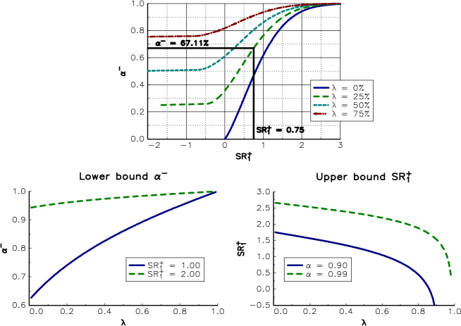
Figure 5: Relationship between $\lambda$, $\mathop{\rm SR}\nolimits\nolimits_{1}^{+}$ and $\alpha^{-}$

This theorem states that the RB portfolio may not exist when $\alpha\leq\max\left(\alpha^{-},\lambda\right)$. In general, $\alpha$ is equal to $99\%$ and $\lambda$ is lower than $25\%$. This case corresponds to a jump every four years. Therefore, the stronger constraint is $\alpha\geq\alpha^{-}$. In Figure 5, we report the relationship between $\alpha^{-}$ and the parameters $\lambda$ and $\mathop{\rm SR}\nolimits\nolimits_{1}^{+}$. We notice that $\alpha^{-}$ is an increasing function of the maximum Sharpe ratio. For instance, if $\lambda$ is equal to $25\%$, the lower bound $\alpha^{-}$ is equal to $67.11\%$ when the maximum Sharpe ratio is equal to $75\%$. In this case, the existence condition is equivalent to:

$$\alpha\geq 67.11\%$$

or:

$$\mathop{\rm SR}\nolimits_{1}^{+}\leq 0.75$$

The worst scenario occurs when the Sharpe ratio of the tangency portfolio is high. In this case, the expected shortfall may be negative, meaning that there is no risk, except if we consider a high confidence level. For example, when we consider a trend-following strategy, the maximum Sharpe ratio may be high at some periods due to important trends. However, in most cases, the vector of expected returns $\mu$ is equal to zero, because the portfolio manager has no views on the future performance of the assets. Therefore, his objective is to build a diversified portfolio. In this case, the maximum Sharpe ratio is equal to zero, implying that there is always a unique solution to the optimization program.

3.3.2 Some examples

To find the numerical solution of the RB portfolio, we use the following optimization program (Roncalli, 2013; Spinu, 2013):

$$y^{\star} = \arg\min\mathop{\rm ES}\nolimits_{\alpha}\left(y\right)-\sum_{i=1}^{n}b_{i}\ln y_{i}$$

u.c. $$y\geq\mathbf{0}$$

The RB portfolio corresponds then to the following weights:

$$x_{i}^{\star}=\frac{y_{i}^{\star}}{\sum_{j=1}^{n}y_{j}^{\star}}$$

Example 2

We consider three assets, whose expected returns are equal to $3\%$, $8\%$ and $12\%$. Their volatilities are equal to $8\%$, $20\%$ and $30\%$ while the correlation matrix of asset returns is provided by the following matrix:

$$\rho=\left(\begin{array}[]{ccc}1.00&&\\ 0.50&1.00&\\ 0.20&0.40&1.00\\ \end{array}\right)$$

For the jumps, we have $\tilde{\mu}_{1}=-15\%$, $\tilde{\mu}_{2}=-40\%$, $\tilde{\mu}_{3}=0\%$, $\tilde{\sigma}_{1}=15\%$, $\tilde{\sigma}_{2}=20\%$ and $\tilde{\sigma}_{3}=10\%$. We also assume that the correlation matrix between the jumps is equal to:

$$\tilde{\rho}=\left(\begin{array}[]{ccc}1.00&&\\ 0.50&1.00&\\ 0.00&0.00&1.00\\ \end{array}\right)$$

Moreover, the intensity $\lambda$ of jumps is equal to $0.25$.

We consider the equal risk contribution (ERC) portfolio where the risk budgets are the same for all the assets. In Table 3, we report the weights of the ERC portfolio when the risk measure is the portfolio’s volatility (Maillard et al., 2010). In this case, the weight of Asset 1 is equal to $60.94\%$ whereas the weight of Asset 3 is equal to $16.87\%$. The difference between the two weights can be explained by the difference in terms of volatility between the three assets. If we use a Gaussian expected shortfall (Roncalli, 2015), the allocation does not change significantly (Table 4). This is normal as the Sharpe ratio of the three assets is similar. However, when we introduce jumps, we note a big impact on the allocation (Table 5). Indeed, Asset 3 is highly volatile, but the risk of jumps is limited. This is not the case for the two other assets. In particular, the skewness risk of Asset 1 is high because its volatility is low, but the expected value of a jump is approximatively five times the expected return in the normal regime. As a result, the allocation is equal to $\left(44.70\%,19.87\%,35.42\%\right)$.

Table 3: ERC portfolio (volatility risk measure)

Asset	$x_{i}$	$\mathcal{MR}_{i}$	$\mathcal{RC}_{i}$	$\mathcal{RC}_{i}^{\star}$
$1$	$60.94$	${\hskip 5.0pt}5.96$	$3.63$	$33.33$
$2$	$22.20$	$16.35$	$3.63$	$33.33$
$3$	$16.87$	$21.52$	$3.63$	$33.33$
$\sigma\left(x\right)$			$10.89$

Table 4: ERC portfolio ($95\%$ Gaussian expected shortfall)

Asset	$x_{i}$	$\mathcal{MR}_{i}$	$\mathcal{RC}_{i}$	$\mathcal{RC}_{i}^{\star}$
$1$	$60.85$	${\hskip 5.0pt}9.24$	$5.62$	$33.33$
$2$	$21.96$	$25.60$	$5.62$	$33.33$
$3$	$17.19$	$32.72$	$5.62$	$33.33$
$\mathop{\rm ES}\nolimits_{\alpha}\left(x\right)$			$16.87$

Table 5: ERC portfolio ($95\%$ expected shortfall with jumps)

Asset	$x_{i}$	$\mathcal{MR}_{i}$	$\mathcal{RC}_{i}$	$\mathcal{RC}_{i}^{\star}$
$1$	$44.70$	$24.70$	$11.04$	$33.33$
$2$	$19.87$	$55.56$	$11.04$	$33.33$
$3$	$35.42$	$31.17$	$11.04$	$33.33$
$\mathop{\rm ES}\nolimits_{\alpha}\left(x\right)$			$33.12$

Remark 2

Using the previous example, we find that $\mathop{\rm SR}\nolimits\nolimits_{1}^{+}=0.52$. It follows that $\alpha^{-}$ is equal to $57.4\%$.

4 Illustration with the equity/bond/volatility asset mix policy

We consider the traditional equity-bond asset mix policy. Nowadays, a lot of investors prefer to use a risk parity portfolio instead of a constant-mix portfolio in order to obtain a risk-balanced allocation between the two assets. While bonds and equities are not Gaussian, it is however accepted that the volatility measure is a good approximation of the risks taken by the investor. Nevertheless, if we introduce a short volatility (or volatility carry) exposure, this assumption is not valid. For instance, we report the cumulative performance of bonds, equities and the short volatility strategy in Figure 6 for the study period January 2000–December 2015. We notice that the short volatility strategy presents a high jump risk compared to bonds and equities. This is confirmed by the extreme returns and statistics of skewness coefficients calculated with different frequencies (see Tables 6 and 7). Indeed, we observe a high asymmetry between best and worst returns for the short volatility strategy. Moreover, the skewness of daily returns is about $-7$ for the volatility carry index, whereas it is close to zero for the bond and equity indices.

Table 6: Best returns, worst returns and maximum drawdown

Asset	Daily	Weekly	Monthly	Annually	Maximum
	Best returns (in %)
Bonds	${\hskip 8.0pt}1.89$	${\hskip 12.0pt}3.06$	${\hskip 12.0pt}7.10$	${\hskip 8.0pt}15.75$
Equities	${\hskip 3.0pt}11.58$	${\hskip 8.0pt}19.21$	${\hskip 8.0pt}22.64$	${\hskip 8.0pt}75.32$
Carry	${\hskip 8.0pt}2.27$	${\hskip 12.0pt}3.13$	${\hskip 12.0pt}4.39$	${\hskip 8.0pt}16.99$
	Worst returns (in %)
Bonds	$-1.67$	$-2.81$	$-4.40$	$-3.41$	$-6.03$
Equities	$-9.03$	$-18.29$	$-29.67$	$-49.69$	$-55.25$
Carry	$-6.82$	$-11.04$	$-23.43$	$-23.37$	$-27.30$

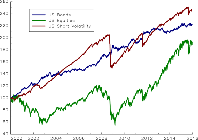
Figure 6: Cumulative performance of US bonds, US equities and US short volatility

Table 7: Skewness coefficients

Asset	Daily	Weekly	Monthly	Annually
Bonds	$-0.12$	$-0.17$	${\hskip 8.0pt}0.07$	${\hskip 8.0pt}0.22$
Equities	${\hskip 8.0pt}0.01$	$-0.44$	$-0.81$	$-0.57$
Carry	$-7.24$	$-5.77$	$-6.32$	$-2.23$

4.1 Estimation of the mixture model

Table 8: Estimation of the Gaussian model (daily model)

Asset	$\mu_{i}$	$\sigma_{i}$	$\rho_{i,j}$
Bonds	$5.54$	${\hskip 5.0pt}4.37$	${\hskip 3.0pt}100.00$
Equities	$6.25$	$20.39$	$-35.06$	$100.00$
Carry	$5.96$	${\hskip 5.0pt}5.62$	$-22.28$	${\hskip 5.0pt}58.07$	$100.00$

In Table 8, we report the maximum likelihood results of the Gaussian model:

$$f\left(y\right)=\phi_{3}\left(y;\mu\,\mathrm{d}t,\Sigma\,\mathrm{d}t\right)$$ (12)

The parameters $\mu$ and $\Sigma$ (expressed in %) are estimated using daily returns. In Appendix B on Page 12, we also give the estimated values of $\mu$ and $\Sigma$ when we consider weekly, monthly and annually overlapping returns. On average, the volatility of US bonds and volatility carry is about $5\%$, whereas the volatility of US equities is $4$ times larger and approximately equal to $20\%$. US bonds have a negative correlation with US equites and volatility carry, which are both positively correlated. We notice that the frequency to compute the returns has an influence on the parameters, but the impact is relatively low, except for the cross-correlations.

We now estimate the Gaussian mixture model with the following parametrization of the probability density function:

$$f\left(y\right)=\left(1-\pi\right)\phi_{1}\left(y;\mu_{1}\,\mathrm{d}t,\sigma_{1}^{2}\,\mathrm{d}t\right)+\pi\phi_{1}\left(y;\mu_{2}\,\mathrm{d}t,\sigma_{2}^{2}\,\mathrm{d}t\right)$$ (13)

We only consider the one-dimensional case in order to illustrate some issues related to the choice of parametrization and frequency. In Figures 7, 8 and 9, we report the estimated values of the parameters $\pi$, $\mu_{1}$, $\mu_{2}$, $\sigma_{1}$ and $\sigma_{2}$. The frequency $\pi$ is large for bonds and equities. These results suggest that a two-volatility regime model is better to describe the returns of equities and bonds than a model with jumps. The first regime is a low volatility environment associated with positive returns, whereas the second regime is a high volatility environment associated with negative returns. In the case of the carry risk premium, the frequency $\pi$ is lower. The large discrepancy between $\mu_{1}$ and $\mu_{2}$, but also between $\sigma_{1}$ and $\sigma_{2}$ justifies that a model with jumps is more relevant than a model with two volatility regimes. Contrary to the standard Gaussian model, the choice of the period for calculating the returns is an important factor. We notice that using one-year returns is not appropriate, because it may produce incoherent results. For instance, the second regime for bonds corresponds to an environment of high returns with low volatility. For the carry risk premium, the volatility is also higher for the first regime than for the second regime. Similarly the case of daily returns is an issue. Indeed, the period may be too short to observe a complete drawdown risk. This is why we prefer to consider a weekly or monthly period to estimate the jump component.

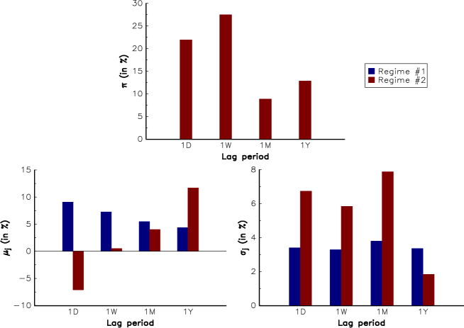
Figure 7: Estimated EM parameters (bonds)

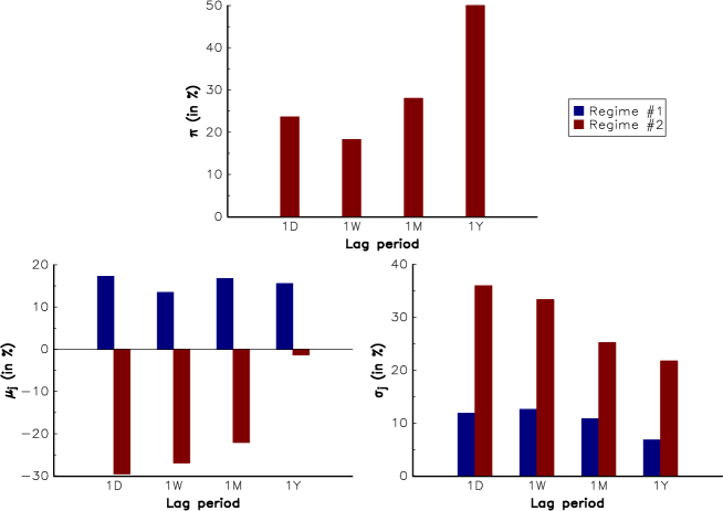
Figure 8: Estimated EM parameters (equities)

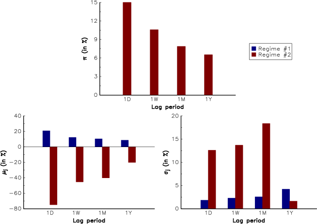
Figure 9: Estimated EM parameters (carry)

Let us consider the multivariate case, where the probability density function is specified as follows:

$$f\left(y\right)=\left(1-\pi\right)\phi_{3}\left(y;\mu\,\mathrm{d}t,\Sigma\,\mathrm{d}t\right)+\pi\phi_{3}\left(y;\mu\,\mathrm{d}t+\tilde{\mu},\Sigma\,\mathrm{d}t+\tilde{\Sigma}\right)$$ (14)

This parametrization ensures that the estimated model is a Gaussian mixture model with a jump component, and not a two-volatility regime model. The reason is that $\Sigma$ is a one-year covariance matrix, whereas $\tilde{\Sigma}$ is a covariance matrix, whose period corresponds to the frequency of calculated returns. Moreover, we assume that $\pi$ is given in order to control the jump frequency. Results are provided in Tables 15 – 18 on Page 15. We confirm that the expected value of the jump $\tilde{\mu}_{i}$ is positive for bonds, whereas it is negative for equities and carry. Moreover, the absolute value of $\tilde{\mu}_{i}$ increases when the jump frequency $\pi$ decreases. For the carry risk premium, we report the probability density function of the jump component in Figure 10. Regarding the dependence of jumps, we notice that the correlations $\tilde{\rho}_{i,j}$ tend to be higher when the jump probability is lower.

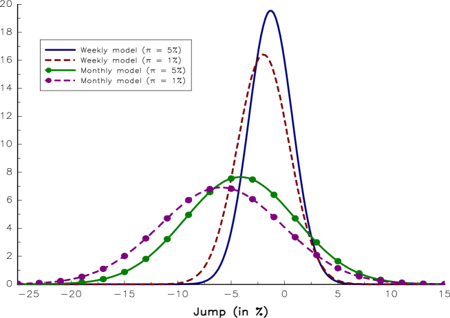
Figure 10: Density function of the jump component (carry)

Remark 3

With the parametrization (14), it is not possible to compare results for different values of the frequency $\mathrm{d}t$. Indeed, fixing $\pi$ at $5\%$ is equivalent to observing a jump every $20$ periods on average. The return period is then approximately equal to five months in the case of weekly returns and one year and eight months in the case of monthly returns. Conversely, if fixing the return period is preferable, it is better to consider the parametrization $\pi=\lambda\,\mathrm{d}t$, where $\lambda$ is the annually jump frequency:

$$f\left(y\right)=\left(1-\lambda\,\mathrm{d}t\right)\phi_{3}\left(y;\mu\,\mathrm{d}t,\Sigma\,\mathrm{d}t\right)+\left(\lambda\,\mathrm{d}t\right)\phi_{3}\left(y;\mu\,\mathrm{d}t+\tilde{\mu},\Sigma\,\mathrm{d}t+\tilde{\Sigma}\right)$$ (15)

In this case, the return period (expressed in years) is equal to $1/\lambda$. For example, if $\lambda$ is equal to $10\%$, the return period of jumps is equal to ten years and we obtain results that are given in Tables 19 and 20 on Page 19.

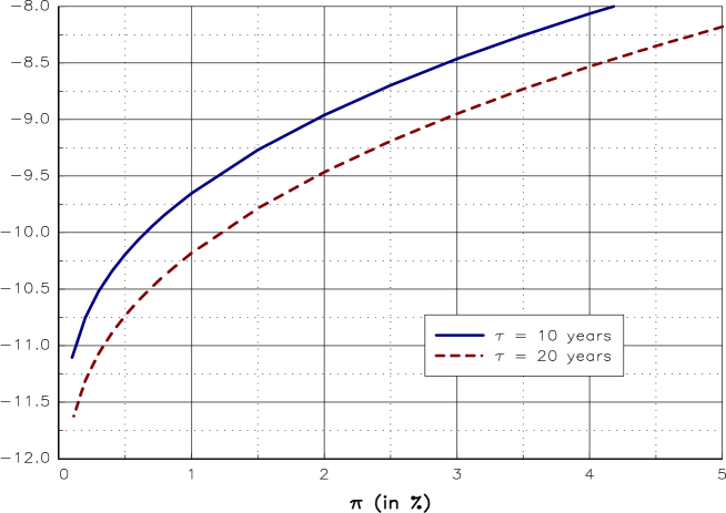
Figure 11: Expected weekly drawdown (in %) of the carry risk premium

In order to deduce the final model, we calculate the expected drawdown associated to a given return period $\tau$:

$$\mathbb{E}\left[\mathop{\rm DD}\nolimits_{i}\left(\tau\right)\right]=\tilde{\mu}_{i}+\Phi^{-1}\left(\frac{\mathrm{d}t}{\tau}\right)\tilde{\sigma}_{i}$$

As the carry strategy constitutes our most skewed asset, it is the only one used in calibrating the parameter $\pi$. Results are reported in Figure 11 for weekly returns. We observe that the expected drawdown is about $-10.5\%$ for $\pi=0.5\%$ when the return period is between 10 and 20 years. This expected drawdown is then close to the worst weekly return observed during the period January 2000 – December 2015 (see Table 6 on Page 6). We also introduce the constraint that bonds have no jump component, because the previous estimations suggest that the expected jump is positive for this asset class. Moreover, it is not statistically significant.

Table 9: Estimation of the constrained mixture model when $\pi=0.5\%$ (weekly model)

Asset	$\mu_{i}$	$\sigma_{i}$	$\rho_{i,j}$
Bonds	${\hskip 8.0pt}5.38$	${\hskip 5.0pt}4.17$	${\hskip 3.0pt}100.00$
Equities	${\hskip 8.0pt}7.89$	$15.64$	$-36.80$	$100.00$
Carry	${\hskip 3.0pt}10.10$	${\hskip 5.0pt}2.91$	$-25.17$	${\hskip 5.0pt}57.43$	$100.00$
Asset	$\tilde{\mu}_{i}$	$\tilde{\sigma}_{i}$	$\tilde{\rho}_{i,j}$
Bonds	${\hskip 8.0pt}0.00$	${\hskip 5.0pt}0.00$	$100.00$
Equities	$-1.20$	${\hskip 5.0pt}6.76$	${\hskip 10.0pt}0.00$	$100.00$
Carry	$-2.23$	${\hskip 5.0pt}2.57$	${\hskip 10.0pt}0.00$	${\hskip 5.0pt}60.45$	$100.00$

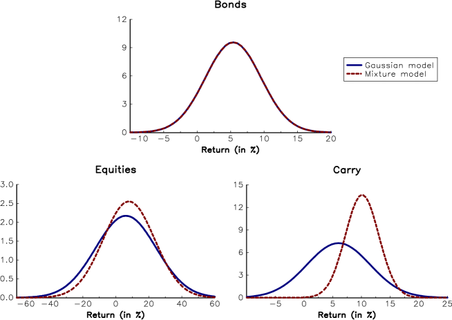
Figure 12: Probability density function of asset returns in the normal regime (weekly model)

Using the method of maximum likelihood, we finally obtain the results given in Table 9. In the case of bonds, we retrieve the results of the Gaussian model (see Table 12 on Page 12). The normal expected return and volatility are equal to $5.38\%$ and $4.17\%$. For equities and the short volatility strategy, the introduction of the jump component increases the expected return and decreases volatility. Indeed, $\mu_{i}$ is respectively equal to $7.89\%$ and $10.10\%$, whereas it was equal to $6.09\%$ and $6.00\%$ in the Gaussian case. The impact on volatility is particularly pronounced for the carry risk premium since it is divided by a factor of $1.9$ ($2.91\%$ versus $5.50\%$). The cross-correlations in the normal regime are close to the values obtained in the Gaussian model. In order to compare the two models, we report the probability density function of asset returns in the normal regime in Figure 12. We confirm that the jump model impacts mainly the modeling of the carry risk premium.

4.2 Comparing in-sample ERC portfolios

We now calculate the ERC portfolio using the $99\%$ expected shortfall risk measure. For that, we use the previous estimates. By construction, we introduce a backtesting bias because the portfolio allocation is based on the full sample of historical data. However, we assume that the expected returns $\mu_{i}$ are equal to zero and not to the historical estimates in order to limit the in-sample bias. In the case of the Gaussian model, we obtain the traditional ERC portfolio based on the volatility risk measure (Maillard et al., 2010). In the case of the weekly model, the allocation is the following: $59.17\%$ in bonds, $10.43\%$ in equities and $30.40\%$ in the short volatility strategy. If we consider the jump model and consider only the normal regime, the allocation becomes: $46.46\%$ in bonds, $9.18\%$ in equities and $44.36\%$ in the short volatility strategy. Therefore, the carry risk premium represents a large part of the portfolio. If we take into account the skewness risk, the allocation is lower and is equal to $36.93\%$. This difference in terms of allocation is even larger when we consider the monthly model. In this case, the allocation for the carry risk premium is $45.58\%$ without jumps and $25.53\%$ with jumps.

Table 10: Weights (in %) of the ERC portfolio

Asset	Weekly model			Monthly model
		Jump model			Jump model
	Gaussian	Normal	Mixture	Gaussian	Normal	Mixture
Bonds	$59.17$	$46.46$	$52.71$	$61.36$	$44.36$	$62.22$
Equities	$10.43$	${\hskip 5.0pt}9.18$	$10.36$	$12.09$	$10.06$	$12.25$
carry	$30.40$	$44.36$	$36.93$	$26.55$	$45.58$	$25.53$

The previous results give the illusion that the Gaussian model is a conservative model and can be compared to the mixture model. This is inaccurate because the results presented are in-sample. For instance, the first major drawdown of the carry strategy occurs in 2008. Before 2008, a Gaussian model will dramatically underestimate the skewness risk of the carry strategy. By considering the full period (January 2000 – December 2015), the covariance matrix of the Gaussian model incorporates these jumps, meaning that the ex-post volatility risk takes into account this skewness risk. To illustrate this bias, we report the one-year rolling volatility of the short volatility strategy in Figure 13. We verify that our estimate largely overestimates the volatility of the carry risk premium in normal periods.

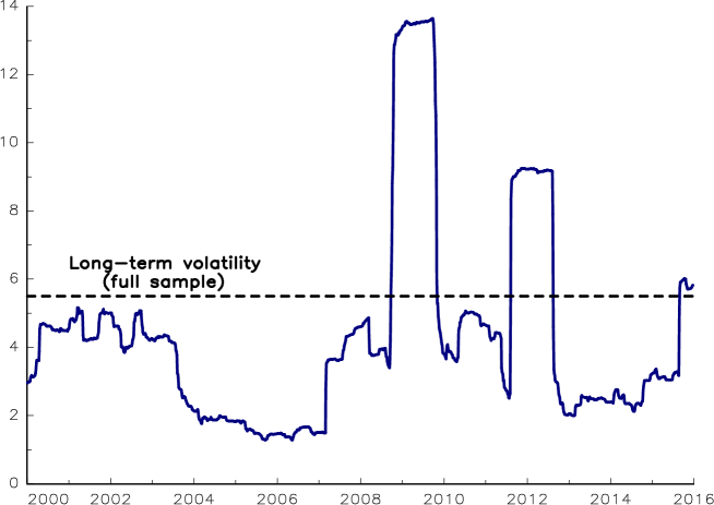
Figure 13: One-year rolling volatility (in %) of the carry risk premium (weekly model)

4.3 Dynamics of out-of-sample ERC portfolios

A more realistic backtest consists in rebalancing the portfolio at a given frequency and to calculate the allocation by using only past data. Therefore, the covariance matrix is no longer static, but time-varying. $\Sigma_{t}$ is then calculated using information until time $t-1$. In the case of the ERC portfolio, it is common to consider a monthly rebalancing based on a one-year rolling covariance matrix. The allocation of the ERC portfolio based on the Gaussian model is reported in Figure 14. We observe that the allocation is not smooth. The weight of the carry risk premium decreases sharply every time there is a jump in asset returns. This negative jump is accompanied by a positive jump in the allocation one year later when the jump in the asset returns exits the rolling window. As a result, we obtain a high turnover and changes in the allocation, which are mainly due to jumps in asset returns.

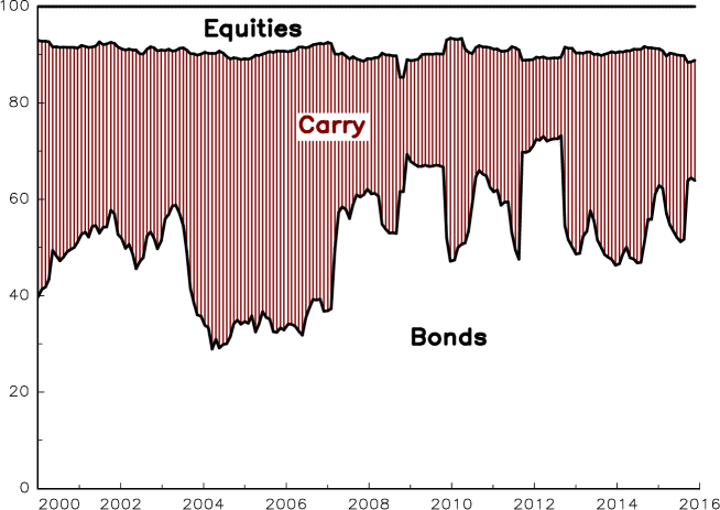
Figure 14: Dynamics of the ERC weights (Gaussian model)

When asset returns exhibit high skewness risk, the drawback of risk parity portfolios is that they reduce the allocation after the occurrence of a jump. However, it is generally too late because jumps are not frequent and not correlated. Moreover, the occurrence of a negative jump is generally followed by a positive performance of the asset. Another drawback of such portfolios is that they will overweight the asset that has no jump over the estimation period, because the risk is underestimated. This implies that the weight will be generally maximum just before the occurrence of a jump.

We now consider the dynamics of the ERC portfolio in the case of our mixture model. We assume that the parameters $\pi$, $\tilde{\mu}$ and $\tilde{\Sigma}$ are given once and for all, and are set to the previous estimates. At each rebalancing date, we have to estimate the covariance matrix $\Sigma_{t}$ for the normal regime. For that, we can apply the method of maximum likelihood to the mixture model with the data of the rolling window:

$$\left(\hat{\mu}_{t},\hat{\Sigma}_{t}\right)=\underset{\left(\mu_{t},\Sigma_{t}\right)}{\arg\max}\sum_{s=1}^{n_{\mathrm{rw}}}\ln\left(\left(1-\pi\right)\phi_{3}\left(R_{t-s},\mu_{t}\,\mathrm{d}t,\Sigma_{t}\,\mathrm{d}t\right)+\pi\phi_{3}\left(R_{t-s},\mu_{t}\,\mathrm{d}t+\tilde{\mu},\Sigma_{t}\,\mathrm{d}t+\tilde{\Sigma}\right)\right)$$

where $n_{\mathrm{rw}}$ is the length of the rolling window. Contrary to the previous analysis, the parameters $\pi$, $\tilde{\mu}$ and $\tilde{\Sigma}$ are not estimated, but are fixed. Only the parameters $\mu_{t}$ and $\Sigma_{t}$ are optimized. The resulting allocation of the ERC portfolio is reported on Page 23.

However, estimating the covariance matrix in the normal regime by maximum likelihood is not our preferred approach. Instead, a popular approach consists in isolating continuous and jump components (Ait-Sahalia and Jacod, 2012). Let $R_{t}$ be the return of one asset. In the thresholding approach, we observe a jump at time $t$ when the absolute return is larger than a given level $r^{\star}$:

$$J_{t}=1\Leftrightarrow\left|R_{t}-v\right|\geq r^{\star}$$

Using a sample of asset returns, we can then create two sub-samples:

• a sub-sample of asset returns without jump that satisfy $\left|R_{t}-v\right|<r^{\star}$;

• a sample of asset returns with jumps that satisfy $\left|R_{t}-v\right|\geq r^{\star}$;

This method is simple and easy to understand. For instance, we can easily estimate the normal volatility by considering the first sub-sample. However, one of the issue is to choose the truncating point $r^{\star}$. Another drawback is that the thresholding approach is only valid in the one-dimensional case. Consequently we prefer to use another approach called the filtering method. In this case, we calculate the posterior probability of the jump regime:

$$\hat{\pi}_{t}=\frac{\pi\phi_{n}\left(R_{t},\mu\,\mathrm{d}t+\tilde{\mu},\Sigma\,\mathrm{d}t+\tilde{\Sigma}\right)}{\left(1-\pi\right)\phi_{n}\left(R_{t},\mu\,\mathrm{d}t,\Sigma\,\mathrm{d}t\right)+\pi\phi_{n}\left(R_{t},\mu\,\mathrm{d}t+\tilde{\mu},\Sigma\,\mathrm{d}t+\tilde{\Sigma}\right)}$$

We will say that we observe a jump at time $t$ when the posterior probability is larger than a threshold $\pi^{\star}$:

$$J_{t}=1\Leftrightarrow\hat{\pi}_{t}\geq\pi^{\star}$$

In Appendix A.7, we show that the filtering procedure is equivalent to the thresholding procedure in the one-dimensional case. However, the thresholding approach is no longer valid in the multi-dimensional case, because the jumps across assets are not necessarily synchronous and the jump regime depends on asset correlations. Moreover, the thresholding rule becomes:

$$J_{t}=1\Leftrightarrow\left(R_{t}-v\right)^{\top}\left(\Sigma\,\mathrm{d}t+\tilde{\Sigma}\right)^{-1}\tilde{\Sigma}\left(\Sigma\,\mathrm{d}t\right)^{-1}\left(R_{t}-v\right)\geq r^{\star}$$

where $v$ and $r^{\star}$ depend on the parameters $\mu$, $\Sigma$, $\tilde{\mu}$ and $\tilde{\Sigma}$. The solution of the thresholding approach is therefore not unique. For this reason, we prefer the filtering approach to detect jumps in the multi-dimensional case.

The filtering method can also be used to estimate the out-of-sample parameters $\hat{\mu}_{t}$ and $\hat{\Sigma}_{t}$. The algorithm is explained in Appendix A.9. The underlying idea is the following:

• Given $\hat{\mu}_{t-1}$ and $\hat{\Sigma}_{t-1}$, we estimate the jump probability for each dates of the rolling window that ends at time $t$;

• Given the previous jump probabilities, we estimate the parameters $\hat{\mu}_{t}$ and $\hat{\Sigma}_{t}$ by only considering the dates of the rolling window, which do not correspond to a jump;

• We iterate the algorithm until today.

The only difficulty is the initialization of the covariance matrix. For that, we consider that there is no jump in the first rolling window. To illustrate the filtering method, we report the jump probability in Figure 15. The in-sample probabilities are calculated using the estimates given in Tables 9 and 21, which have been obtained using the full sample. The out-of-sample probabilities correspond to the average of posterior probabilities, which are calculated using the filtering algorithm, a one-year rolling window and $\pi^{\star}=30\%$.

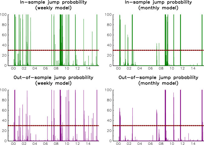
Figure 15: Jump probabilities (in %)

Remark 4

In Markov regime-switching models, in-sample probabilities are called smoothing probabilities, whereas out-of-sample probabilities are called filtering probabilities.

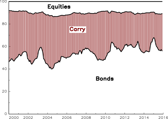
Figure 23: Dynamics of the ERC weights (mixture model, ML method)

We notice some differences between smoothing and filtering probabilities. One reason is that filtering probabilities depend on the value taken by $\pi^{\star}$. If we use a small value, we will delete a lot of observations when computing $\hat{\mu}_{t}$ and $\hat{\Sigma}_{t}$. Therefore, the covariance matrix will be underestimated implying that the jump probabilities will be higher. The opposite is also true. The choice of $\pi^{\star}$ is then a key factor. In Figure 15, we observe that some jumps detected by the smoothing procedure are not identified by the filtering algorithm. This explains that the filtering volatility of the carry risk premium is slightly overestimated with respect to the smoothing volatility (see Figure 16). However, the filtering procedure appears as a robust out-of-sample method if we compare rolling and filtering volatilities. Moreover, it produces an allocation (Figure 17) that is close to the one obtained by the maximum likelihood approach (see Figure 23 on Page 23).

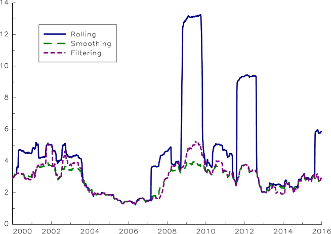
Figure 16: Estimated volatility (in %) of the carry risk premium (weekly model)

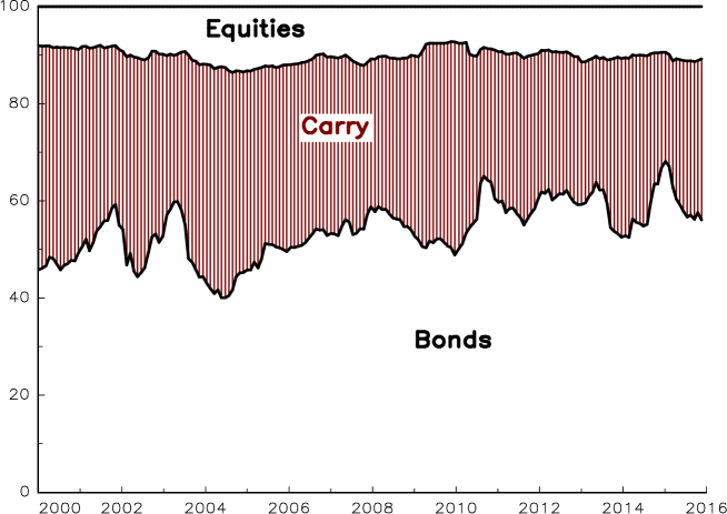
Figure 17: Dynamics of the ERC weights (mixture model, filtering method)

4.4 Analysis of the results

If we compare the previous out-of-sample ERC portfolios calculated using the volatility risk measure and the skewness risk measure; we obtain the following results:

• The annual turnover of the skewness-based ERC allocation is $40\%$ lower than the annual turnover of the volatility-based ERC allocation.

• This additional turnover is mainly explained by the jumps of the short volatility strategy. In Figure 18, we report the cumulative performance of the carry risk premium and the weights in the ERC portfolios. In the case of the volatility-based ERC allocation, we notice that each time we observe a jump, the volatility-based weight decreases dramatically. One year later after the jump, the weight highly increases because the jump falls outside the rolling window.

• In terms of historical performance, volatility and Sharpe ratio, the two portfolios are equivalent. However, we observe two different periods. Before 2008, the volatility-based ERC portfolio largely outperforms the skewness-based ERC portfolio (28 bps more in terms of Sharpe ratio). Since 2008, the opposite is true.

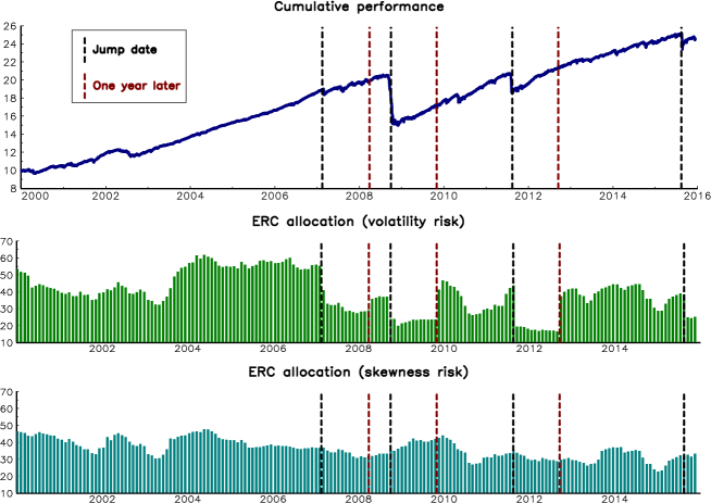
Figure 18: Comparison of the carry allocation (weekly model)

5 Application to factor investing and alternative risk premia

The extensive study on the equity/bond/volatility asset mix policy in the previous section shows how the properties of risk parity portfolios can be improved by taking into account skewness or jump risk. This is particularly true if we consider transaction costs. Indeed, the volatility-based risk parity portfolio reduces dramatically the allocation of one asset immediately after the jump. In this situation, portfolio rebalancing happens in a period of stress and there is no guarantee that market liquidity will be enough to ensure fair bid-ask spreads or even execute the sell order.

Nowadays, the traditional risk parity portfolio (and especially the equal risk contribution portfolio) has become the standard approach for allocating between risk premia, far ahead mean-variance optimized portfolios (Maeso and Martellini, 2016). In the case of standard and liquid assets, this approach is robust. Indeed, the drawdowns of these assets are generally in line with their volatility. This concerns equities, investment grade bonds and commodities. However, as illustrated in this article, traditional risk-based portfolios are not necessarily optimal investments when assets present high skewness risk. This is the case of the short volatility strategy, but also other alternative risk premia like equity size and value risk factors. This is also true with illiquid assets or low liquidity strategies like the credit carry risk premium and some leveraged relative value strategies.

5.1 Factor investing

Equity factor investing is a typical example of skewness risk. It consists in building a diversified portfolio using the more relevant long-only equity risk factors (size, value, momentum, low beta and quality). This portfolio combines then two pure (or skewness) risk premia – size and value – and three market anomalies – momentum, low beta and quality (Cazalet and Roncalli, 2014). The risk parity portfolio allocates the same volatility risk to the five risk factors. However, the risk parity portfolio ignores two main risks which are difficult to measure using the volatility risk measure (Hamdan et al., 2016):

• The value strategy faces a distressed risk due to the default risk of value stocks. An example was the impact of the Lehman Brothers bankruptcy on the performance of value portfolios at the end of 2008.

• The size risk premium also faces a distressed risk due to the liquidity risk of small cap stocks. For instance, the period of low liquidity between June 2008 and March 2009 has weighted on the performance of the size factor.

By using the framework developed here, we show that the size and value allocation is generally overestimated in factor-based investing, because the portfolio construction does not take into account the skewness risk.

5.2 Skewness risk premia

By construction, our framework is particularly relevant for managing a portfolio of assets that incorporates skewness risk premia. The equity/bond/volatility asset mix policy is an emblematic illustration, because the short volatility strategy is one of the most famous example of skewness risk. We may also consider other asset allocation problems, like the portfolio of cross-asset carry risk premia or the introduction of less liquid strategies. Another example concerns the equity cross-section momentum risk premium. In a long/short format, this risk premium is subject to a high skewness risk known as momentum crashes (Daniel and Moskowitz, 2016). In this context, a volatility-based risk parity portfolio overestimates the allocation of such risk premium. Moreover, our analysis shows that this result depends on the implementation of the momentum risk factor. In particular, the overestimation is more salient for the winners-minus-losers strategy than for the winners-minus-market strategy.

5.3 Volatility hedging versus skewness hedging

Hamdan et al. (2016) noticed that “there is a floor to the hedging of the third moment, which is not the case for the second moment. As a consequence, volatility diversification or negative correlation leads to reduced volatility, but increased tail risks in relative terms”. Using the equity/bond/carry example, we confirm that skewness hedging is a difficult task. In table 11, we report the composition of some risk-based portfolios using the estimates of the weekly model. Using the Gaussian model, the minimum variance (MV) portfolio is composed of $63.26\%$ of bonds, $2.23\%$ of equities and $34.51\%$ of the carry risk premium. The volatility and the skewness of the MV portfolio are then equal to $2.62\%$ and $-2.75$. If we consider the normal regime of the mixture model and compute the MV portfolio, the weights become $36.06\%$ for bonds, $0\%$ for equities and $63.95\%$ for the carry risk premium. In both cases, the MV portfolio has a low or zero allocation in equities, because this asset class is highly volatile. The allocation in the short volatility strategy is high when we consider the normal regime. This is the most frequent situation because jumps are rare. However, the portfolio is also highly risky because skewness is equal to $-19.81$!. We have also computed the minimum expected shortfall (MES) portfolio at the $99\%$ confidence level in the last column. In this case, the portfolio is fully invested in bonds. Therefore, we notice a big difference between MV and MES portfolios. Minimizing the volatility leads then to allocating a large part in the carry risk premium, whereas minimizing the expected shortfall implies replacing this asset by bonds. By focusing on volatility, the investor may then neglect the skewness risk. Moreover, this risk cannot be diversified contrary to the volatility risk. These results explain that life performance of risk factor and alternatives risk premia portfolios are not always in line with the performance of their (in-sample) backtests.

Table 11: Volatility and skewness risks of risk-based portfolios (weekly model)

Portfolio	MV	MV	ERC	MES
Model	Gaussian	Jump model
	(full sample)	Normal	Mixture	Mixture
Bonds	${\hskip 3.0pt}63.26\%$	${\hskip 8.0pt}36.05\%$	${\hskip 3.0pt}52.71\%$	$100.00\%$
Equities	${\hskip 8.0pt}2.23\%$	${\hskip 13.0pt}0.00\%$	${\hskip 3.0pt}10.36\%$	${\hskip 10.0pt}0.00\%$
Carry	${\hskip 3.0pt}34.51\%$	${\hskip 8.0pt}63.95\%$	${\hskip 3.0pt}36.93\%$	${\hskip 10.0pt}0.00\%$
$\sigma\left(x\right)$	${\hskip 8.0pt}2.62\%$	${\hskip 13.0pt}2.33\%$	${\hskip 8.0pt}2.75\%$	${\hskip 10.0pt}4.17\%$
$\gamma_{1}$	$-2.75{\hskip 8.0pt}$	$-19.81{\hskip 8.0pt}$	$-6.17{\hskip 8.0pt}$	${\hskip 10.0pt}0.00{\hskip 8.0pt}$

Remark 5

Some investors think that CTA is a good strategy for hedging the skewness risk. This belief comes from the 2008 financial crisis, when CTA has posted positive returns while the drawdown of the equity market was large. In fact, there is a confusion between two risks: the CTA strategy has done a good job in hedging the volatility risk, not the skewness risk. Indeed, the 2008 financial crisis is more an event of high volatility risk than an episode of pure skewness risk. This explains that the performance of CTA is generally disappointing when skewness risks occur (e.g. 2011, January 2015, etc.)

6 Conclusion

This paper may be viewed as the end of a trilogy, which started with the study of factor investing (Cazalet and Roncalli, 2014) and was extended with the analysis of alternative risk premia (Hamdan et al., 2016). The two previous analysis have shown the importance of skewness risk in the universe of risk premia and confirmed the asymmetric tail risks of some strategies (Lempérière et al., 2014). This is particularly true for skewness risk premia, which may exhibit extreme jump movements.

As shown by Hamdan et al. (2016), it is an illusion to think that we can fully hedge the skewness risk, because there is a floor to skewness diversification. In this paper, we present a new risk-based model, whose objective is to take into account these limits. Our framework uses the risk budgeting approach by considering the expected shortfall measure instead of the volatility risk measure. However, contrary to Roncalli (2015) who assumed that asset returns are Gaussian, we use a mixture distribution with two regimes for modeling asset returns. The first regime is normal whereas the second regime incorporates jumps. This model allows us to obtain closed-form formulas for risk contributions, and we can then compute risk-based portfolios.

To illustrate the model, we consider the traditional equity/bond asset mix policy by introducing the short volatility strategy, which is a highly skewed asset. The comparison of volatility-based and skewness-based risk parity portfolios showed that traditional risk-based portfolios give too much weight to skewed assets in periods of calm. Skewness-based risk parity portfolios are more robust and remain invested in skewed assets once the jump risk has been observed. This example shows that hedging the skewness is a difficult task. Because the skewness is a statistical measure of jumps, skewness hedging is equivalent to jump hedging. However, contrary to the volatility, we show that jumps are difficult to hedge. In particular, volatility diversification and optimization can produce portfolios, which present low volatility risk but high stress risk. This is why skewness diversification is an illusion. The appropriate answer is then to size the position of the skewed asset according to its real risk, and not only to its volatility risk. This result is important for institutional investors and pension funds managing portfolios of equity risk factors or alternative risk premia. More generally, our results question the strategic asset allocation when it includes skewed and illiquid assets. It is of course the case of hedge fund strategies (Billio et al., 2012), but also other alternative assets like credit, real estate or infrastructure.

Appendix A Mathematical results

A.1 Characteristic function of the jump-diffusion process

We know that the characteristic function of the compound Poisson process $Z_{t}$ has the following expression:

$$\mathbb{E}\left[e^{-iu.Z_{t}}\right]=e^{\lambda t\left(F\left(u\right)-1\right)}$$

where $F\left(u\right)=\exp\left(iu^{\top}\tilde{\mu}-\frac{1}{2}u^{\top}\tilde{\Sigma}u\right)$ is the characteristic function of jump amplitudes. It follows that the characteristic function of the Lévy process $\mathrm{d}L_{t}$ is equal to:

$$\mathbb{E}\left[e^{-iu.\mathrm{d}L_{t}}\right]=e^{\left(iu^{\top}\mu-\frac{1}{2}u^{\top}\Sigma u\right)\,\mathrm{d}t+\lambda\left(F\left(u\right)-1\right)\,\mathrm{d}t}$$

If we assume $\lambda\,\mathrm{d}t$ small enough (or alternatively that $\lambda$ is small), we can make the following approximation:

$$\mathbb{E}\left[e^{-iu.\mathrm{d}L_{t}}\right] \approx\left(1+\lambda\,\mathrm{d}t\left(F\left(u\right)-1\right)\right)e^{\left(iu^{\top}\mu-\frac{1}{2}u^{\top}\Sigma u\right)\,\mathrm{d}t}$$

$$\approx\left(1-\lambda\,\mathrm{d}t\right)\cdot e^{\left(iu^{\top}\mu-\frac{1}{2}u^{\top}\Sigma u\right)\,\mathrm{d}t}+\left(\lambda\,\mathrm{d}t\right)\cdot e^{\left(iu^{\top}\mu-\frac{1}{2}u^{\top}\Sigma u\right)\,\mathrm{d}t}e^{iu^{\top}\tilde{\mu}-\frac{1}{2}u^{\top}\tilde{\Sigma}u}$$

Finally, we obtain:

$$\mathbb{E}\left[e^{-iu.\mathrm{d}L_{t}}\right]\approx\left(1-\lambda\,\mathrm{d}t\right)\cdot e^{\left(iu^{\top}\mu-\frac{1}{2}u^{\top}\Sigma u\right)\,\mathrm{d}t}+\left(\lambda\,\mathrm{d}t\right)\cdot e^{iu^{\top}\left(\mu\,\mathrm{d}t+\tilde{\mu}\right)-\frac{1}{2}u^{\top}\left(\Sigma\,\mathrm{d}t+\tilde{\Sigma}\right)u\ }$$

A.2 Skewness of Gaussian mixture models

We consider the mixture $Y$ of two normal random variables $Y_{1}$ and $Y_{2}$, whose distribution function is:

$$f\left(y\right)=\pi_{1}f_{1}\left(y\right)+\pi_{2}f_{2}\left(y\right)$$

where $Y_{1}\sim\mathcal{N}\left(\mu_{1},\sigma_{1}^{2}\right)$, $Y_{2}\sim\mathcal{N}\left(\mu_{2},\sigma_{2}^{2}\right)$ and $\pi_{1}+\pi_{2}=1$. The $k$-th moment of $Y$ is given by:

$$\mathbb{E}\left[Y^{k}\right]=\pi_{1}\mathbb{E}\left[Y_{1}^{k}\right]+\pi_{2}\mathbb{E}\left[Y_{2}^{k}\right]$$

We know that $\mathbb{E}\left[Y_{i}\right]=\mu_{i}$, $\mathbb{E}\left[Y_{i}^{2}\right]=\mu_{i}^{2}+\sigma_{i}^{2}$ and $\mathbb{E}\left[Y_{i}^{3}\right]=\mu_{i}^{3}+3\mu_{i}\sigma_{i}^{2}$. We deduce that:

$$\mathbb{E}\left[Y\right]=\pi_{1}\mu_{1}+\pi_{2}\mu_{2}$$

and:

$$\sigma^{2}\left(Y\right) = \pi_{1}\mathbb{E}\left[Y_{1}^{2}\right]+\pi_{2}\mathbb{E}\left[Y_{2}^{2}\right]-\mathbb{E}^{2}\left[Y\right]$$

$$= \pi_{1}\left(\mu_{1}^{2}+\sigma_{1}^{2}\right)+\pi_{2}\left(\mu_{2}^{2}+\sigma_{2}^{2}\right)-\left(\pi_{1}\mu_{1}+\pi_{2}\mu_{2}\right)^{2}$$

$$= \pi_{1}\sigma_{1}^{2}+\pi_{2}\sigma_{2}^{2}+\pi_{1}\left(1-\pi_{1}\right)\left(\mu_{1}^{2}+\mu_{2}^{2}\right)-2\pi_{1}\pi_{2}\mu_{1}\mu_{2}$$

$$= \pi_{1}\sigma_{1}^{2}+\pi_{2}\sigma_{2}^{2}+\pi_{1}\pi_{2}\left(\mu_{1}-\mu_{2}\right)^{2}$$

because $\pi_{2}=1-\pi_{1}$. Recall that the skewness coefficient of $Y$ has the following expression:

$$\gamma_{1}\left(Y\right)=\mathbb{E}\left[\left(\frac{Y-\mathbb{E}\left[Y\right]}{\sigma\left(Y\right)}\right)^{3}\right]$$

It follows:

$$\mathbb{E}\left[\left(Y-\mathbb{E}\left[Y\right]\right)^{3}\right] = \mathbb{E}\left[Y^{3}\right]-3\mathbb{E}\left[Y\right]\sigma^{2}\left(Y\right)-\mathbb{E}^{3}\left[Y\right]$$

$$= \pi_{1}\left(\mu_{1}^{3}+3\mu_{1}\sigma_{1}^{2}\right)+\pi_{2}\left(\mu_{2}^{3}+3\mu_{2}\sigma_{2}^{2}\right)-$$

$$3\left(\pi_{1}\mu_{1}+\pi_{2}\mu_{2}\right)\left(\pi_{1}\sigma_{1}^{2}+\pi_{2}\sigma_{2}^{2}+\pi_{1}\pi_{2}\left(\mu_{1}-\mu_{2}\right)^{2}\right)-$$

$$\left(\pi_{1}\mu_{1}+\pi_{2}\mu_{2}\right)^{3}$$

$$= \pi_{1}\pi_{2}\left(\pi_{2}-\pi_{1}\right)\left(\mu_{1}-\mu_{2}\right)^{3}+3\pi_{1}\pi_{2}\left(\mu_{1}-\mu_{2}\right)\left(\sigma_{1}^{2}-\sigma_{2}^{2}\right)$$

We deduce:

$$\gamma_{1}\left(Y\right)=\frac{\pi_{1}\pi_{2}\left(\left(\pi_{2}-\pi_{1}\right)\left(\mu_{1}-\mu_{2}\right)^{3}+3\left(\mu_{1}-\mu_{2}\right)\left(\sigma_{1}^{2}-\sigma_{2}^{2}\right)\right)}{\left(\pi_{1}\sigma_{1}^{2}+\pi_{2}\sigma_{2}^{2}+\pi_{1}\pi_{2}\left(\mu_{1}-\mu_{2}\right)^{2}\right)^{\nicefrac{{3}}{{2}}}}$$ (16)

A.3 Derivation of the EM algorithm

The log-likelihood function is:

$$\ell\left(\theta\right)=\sum_{t=1}^{T}\ln\sum_{j=1}^{2}\pi_{j}\phi_{n}\left(R_{t};\mu_{j},\Sigma_{j}\right)$$

The derivative of $\ell\left(\theta\right)$ with respect to $\mu_{j}$ is equal to:

$$\frac{\partial\,\ell\left(\theta\right)}{\partial\,\mu_{j}}=\sum_{t=1}^{T}\frac{\pi_{j}\phi_{n}\left(R_{t};\mu_{j},\Sigma_{j}\right)}{\sum_{s=1}^{2}\pi_{s}\phi_{n}\left(R_{t};\mu_{s},\Sigma_{s}\right)}\Sigma_{j}^{-1}\left(R_{t}-\mu_{j}\right)$$

Therefore, the first-order condition is:

$$\sum_{t=1}^{T}\pi_{j,t}\Sigma_{j}^{-1}\left(R_{t}-\mu_{j}\right)=\mathbf{0}$$

where:

$$\pi_{j,t}=\frac{\pi_{j}\phi_{n}\left(R_{t};\mu_{j},\Sigma_{j}\right)}{\sum_{s=1}^{2}\pi_{s}\phi_{n}\left(R_{t};\mu_{s},\Sigma_{s}\right)}$$

We deduce the expression of the estimator $\hat{\mu}_{j}$:

$$\hat{\mu}_{j}=\frac{\sum_{t=1}^{T}\pi_{j,t}R_{t}}{\sum_{t=1}^{T}\pi_{j,t}}$$ (17)

For the derivative with respect to $\Sigma_{j}$, we consider the function $g\left(\Sigma_{j}^{-1}\right)$ defined as follows:

$$g\left(\Sigma_{j}^{-1}\right) = \frac{1}{\left(2\pi\right)^{n/2}\left|\Sigma_{j}\right|^{1/2}}e^{-\frac{1}{2}\left(R_{t}-\mu_{j}\right)^{\top}\Sigma_{j}^{-1}\left(R_{t}-\mu_{j}\right)}$$

$$= \frac{\left|\Sigma_{j}^{-1}\right|^{1/2}}{\left(2\pi\right)^{n/2}}e^{-\frac{1}{2}\mathop{\rm trace}\left(\Sigma_{j}^{-1}\left(R_{t}-\mu_{j}\right)\left(R_{t}-\mu_{j}\right)^{\top}\right)}$$

It follows:

$$\frac{\partial\,g\left(\Sigma_{j}^{-1}\right)}{\partial\,\Sigma_{j}^{-1}} = \frac{1}{2}\frac{\left|\Sigma_{j}^{-1}\right|^{-1/2}\left|\Sigma_{j}^{-1}\right|\Sigma_{j}}{\left(2\pi\right)^{n/2}}e^{-\dfrac{1}{2}\mathop{\rm trace}\left(\Sigma_{j}^{-1}\left(R_{t}-\mu_{j}\right)\left(R_{t}-\mu_{j}\right)^{\top}\right)}$$

$$-\frac{1}{2}\left(R_{t}-\mu_{j}\right)\left(R_{t}-\mu_{j}\right)^{\top}\frac{\left|\Sigma_{j}^{-1}\right|^{1/2}}{\left(2\pi\right)^{n/2}}e^{-\dfrac{1}{2}\mathop{\rm trace}\left(\Sigma_{j}^{-1}\left(R_{t}-\mu_{j}\right)\left(R_{t}-\mu_{j}\right)^{\top}\right)}$$

$$= \frac{1}{\left(2\pi\right)^{n/2}\left|\Sigma_{j}\right|^{1/2}}e^{-\dfrac{1}{2}\left(R_{t}-\mu_{j}\right)\Sigma_{j}^{-1}\left(R_{t}-\mu_{j}\right)^{\top}}\frac{\left(\Sigma_{j}-\left(R_{t}-\mu_{j}\right)\left(R_{t}-\mu_{j}\right)^{\top}\right)}{2}$$

We deduce:

$$\frac{\partial\,\ell\left(\theta\right)}{\partial\,\Sigma_{j}^{-1}}=\frac{1}{2}\sum_{t=1}^{T}\frac{\pi_{j}\phi_{n}\left(R_{t};\mu_{j},\Sigma_{j}\right)}{\sum_{s=1}^{2}\pi_{s}\phi_{n}\left(R_{t};\mu_{s},\Sigma_{s}\right)}\left(\Sigma_{j}-\left(R_{t}-\mu_{j}\right)\left(R_{t}-\mu_{j}\right)^{\top}\right)$$

The first-order condition is then:

$$\sum_{t=1}^{T}\pi_{j,t}\left(\Sigma_{j}-\left(R_{t}-\mu_{j}\right)\left(R_{t}-\mu_{j}\right)^{\top}\right)=0$$

It follows that the estimator $\hat{\Sigma}_{j}$ is equal to:

$$\hat{\Sigma}_{j}=\frac{\sum_{t=1}^{T}\pi_{j,t}\left(R_{t}-\hat{\mu}_{j}\right)\left(R_{t}-\hat{\mu}_{j}\right)^{\top}}{\sum_{t=1}^{T}\pi_{j,t}}$$ (18)

Regarding the mixture probabilities $\pi_{j}$, the first-order condition implies:

$$\sum_{t=1}^{T}\frac{\phi_{n}\left(R_{t};\mu_{j},\Sigma_{j}\right)}{\sum_{s=1}^{2}\pi_{s}\phi_{n}\left(R_{t};\mu_{s},\Sigma_{s}\right)}=c$$

where $c$ is the Lagrange multiplier associated to the constraint $\sum_{j=1}^{2}\pi_{j}=1$. We deduce that $c=T$. We conclude that it is not possible to directly define the estimator $\hat{\pi}_{j}$. This is why we have to use another route to obtain the ML estimators.

We introduce the estimator $\hat{\pi}_{j,t}$:

$$\hat{\pi}_{j,t}=\frac{\pi_{j}\phi_{n}\left(R_{t};\mu_{j},\Sigma_{j}\right)}{\sum_{s=1}^{2}\pi_{s}\phi_{n}\left(R_{t};\mu_{s},\Sigma_{s}\right)}$$ (19)

$\hat{\pi}_{j,t}$ is the posterior probability of the regime index for the observation $t$. Knowing $\hat{\pi}_{j,t}$, the estimator $\hat{\pi}_{j}$ is given by:

$$\hat{\pi}_{j}=\frac{\sum_{t=1}^{T}\hat{\pi}_{j,t}}{T}$$ (20)

The EM algorithm consists in the following iterations:

1. Initialize the algorithm with starting values $\pi_{j}^{\left(0\right)}$, $\mu_{j}^{\left(0\right)}$ and $\Sigma_{j}^{\left(0\right)}$; Set $k=0$.

2. Using Equation (19), we calculate the posterior probabilities $\pi_{j,t}$:

   $$\pi_{j,t}^{\left(k\right)}=\frac{\pi_{j}^{\left(k\right)}\phi_{n}\left(R_{t};\mu_{j}^{\left(k\right)},\Sigma_{j}^{\left(k\right)}\right)}{\sum_{s=1}^{2}\pi_{s}^{\left(k\right)}\phi_{n}\left(R_{t};\mu_{s}^{\left(k\right)},\Sigma_{s}^{\left(k\right)}\right)}$$

3. Using Equations (20), (17) and (18), we update the estimators $\hat{\pi}_{j}$, $\hat{\mu}_{j}$ and $\hat{\Sigma}_{j}$:

   $$\pi_{j}^{\left(k+1\right)} = \frac{\sum_{t=1}^{T}\pi_{j,t}^{\left(k\right)}}{T}$$

   $$\mu_{j}^{\left(k+1\right)} = \frac{\sum_{t=1}^{T}\pi_{j,t}^{\left(k\right)}R_{t}}{\sum_{t=1}^{T}\pi_{j,t}^{\left(k\right)}}$$

   $$\Sigma_{j}^{\left(k+1\right)} = \frac{\sum_{t=1}^{T}\pi_{j,t}^{\left(k\right)}\left(R_{t}-\mu_{j}^{\left(k+1\right)}\right)\left(R_{t}-\mu_{j}^{\left(k+1\right)}\right)^{\top}}{\sum_{t=1}^{T}\pi_{j,t}^{\left(k\right)}}$$

4. We iterate Steps 2 and 3 until convergence.

5. Finally, we have $\hat{\pi}_{j}=\pi_{j}^{\left(\infty\right)}$, $\hat{\mu}_{j}=\pi_{j}^{\left(\infty\right)}$ and $\hat{\Sigma}_{j}=\Sigma_{j}^{\left(\infty\right)}$.

A.4 Expression of the expected shortfall

Let $Y\sim\mathcal{N}\left(\mu,\sigma^{2}\right)$ be a Gaussian random variable. We consider the following quantity:

$$\varphi=\mathbb{E}\left[\mathds{1}\left\{Y\geq a\right\}\cdot Y\right]$$

We have:

$$\varphi = \int_{a}^{\infty}\frac{y}{\sigma}\phi\left(\frac{y-\mu}{\sigma}\right)\,\mathrm{d}y$$

$$= \int_{\sigma^{-1}\left(a-\mu\right)}^{\infty}\left(\mu+\sigma t\right)\phi\left(t\right)\,\mathrm{d}t$$

$$= \mu\left[\Phi\left(t\right)\right]_{\sigma^{-1}\left(a-\mu\right)}^{\infty}+\frac{\sigma}{\sqrt{2\pi}}\int_{\sigma^{-1}\left(a-\mu\right)}^{\infty}t\exp\left(-\frac{1}{2}t^{2}\right)\,\mathrm{d}t$$

$$= \mu\left(1-\Phi\left(\frac{a-\mu}{\sigma}\right)\right)+\frac{\sigma}{\sqrt{2\pi}}\left[-\exp\left(-\frac{1}{2}t^{2}\right)\right]_{\sigma^{-1}\left(a-\mu\right)}^{\infty}$$

$$= \mu\Phi\left(-\frac{a-\mu}{\sigma}\right)+\sigma\phi\left(\frac{a-\mu}{\sigma}\right)$$

In the case of the model with jumps, the definition of the expected shortfall is:

$$\mathop{\rm ES}\nolimits_{\alpha}\left(x\right)=\mathbb{E}\left[L\left(x\right)\mid L\left(x\right)\geq\mathop{\rm VaR}\nolimits_{\alpha}\left(x\right)\right]$$

where $L(x)=-R(x)$ is the portfolio’s loss. It follows that:

$$\mathop{\rm ES}\nolimits_{\alpha}\left(x\right) = \frac{1}{1-\alpha}\cdot\mathbb{E}\left[\mathds{1}\left\{L\left(x\right)\geq\mathop{\rm VaR}\nolimits_{\alpha}\left(x\right)\right\}\cdot L\left(x\right)\right]$$

$$= \frac{1}{1-\alpha}\int_{\mathop{\rm VaR}\nolimits_{\alpha}\left(x\right)}^{\infty}yg\left(y\right)\,\mathrm{d}y$$

where $g\left(y\right)$ is the density function of $L\left(x\right)$. Using Equation (3), we have:

$$g\left(y\right)=\left(1-\lambda\right)\frac{1}{\sigma_{1}\left(x\right)}\phi\left(\frac{y+\mu_{1}\left(x\right)}{\sigma_{1}\left(x\right)}\right)+\lambda\frac{1}{\sigma_{2}\left(x\right)}\phi\left(\frac{y+\mu_{2}\left(x\right)}{\sigma_{2}\left(x\right)}\right)$$

We deduce:

$$\int_{\mathop{\rm VaR}\nolimits_{\alpha}\left(x\right)}^{\infty}yg\left(y\right)\,\mathrm{d}y = \left(1-\lambda\right)\cdot\mathbb{E}\left[\mathds{1}\left\{L_{1}\left(x\right)\geq\mathop{\rm VaR}\nolimits_{\alpha}\left(x\right)\right\}\cdot L_{1}\left(x\right)\right]+$$

$$\lambda\cdot\mathbb{E}\left[\mathds{1}\left\{L_{2}\left(x\right)\geq\mathop{\rm VaR}\nolimits_{\alpha}\left(x\right)\right\}\cdot L_{2}\left(x\right)\right]$$

where $L_{1}\left(x\right)\sim\mathcal{N}\left(-\mu_{1}\left(x\right),\sigma_{1}^{2}\left(x\right)\right)$ and $L_{2}\left(x\right)\sim\mathcal{N}\left(-\mu_{2}\left(x\right),\sigma_{2}^{2}\left(x\right)\right)$. Finally, we obtain:

$$\mathop{\rm ES}\nolimits_{\alpha}\left(x\right) = \frac{1-\lambda}{1-\alpha}\left(\sigma_{1}\left(x\right)\phi\left(\frac{\mathop{\rm VaR}\nolimits_{\alpha}\left(x\right)+\mu_{1}\left(x\right)}{\sigma_{1}\left(x\right)}\right)-\mu_{1}\left(x\right)\Phi\left(-\frac{\mathop{\rm VaR}\nolimits_{\alpha}\left(x\right)+\mu_{1}\left(x\right)}{\sigma_{1}\left(x\right)}\right)\right)+$$

$$\frac{\lambda}{1-\alpha}\left(\sigma_{2}\left(x\right)\phi\left(\frac{\mathop{\rm VaR}\nolimits_{\alpha}\left(x\right)+\mu_{2}\left(x\right)}{\sigma_{2}\left(x\right)}\right)-\mu_{2}\left(x\right)\Phi\left(-\frac{\mathop{\rm VaR}\nolimits_{\alpha}\left(x\right)+\mu_{2}\left(x\right)}{\sigma_{2}\left(x\right)}\right)\right)$$

This expression depends on the value taken by the value-at-risk, which is defined by:

$$\Pr\left\{L\left(x\right)\leq\mathop{\rm VaR}\nolimits_{\alpha}\left(x\right)\right\}=\alpha$$

It follows:

$$\int_{-\infty}^{\mathop{\rm VaR}\nolimits_{\alpha}\left(x\right)}g\left(y\right)\,\mathrm{d}y=\alpha$$

or:

$$\left(1-\lambda\right)\cdot\Phi\left(\frac{\mathop{\rm VaR}\nolimits_{\alpha}\left(x\right)+\mu_{1}\left(x\right)}{\sigma_{1}\left(x\right)}\right)+\lambda\cdot\Phi\left(\frac{\mathop{\rm VaR}\nolimits_{\alpha}\left(x\right)+\mu_{2}\left(x\right)}{\sigma_{2}\left(x\right)}\right)=\alpha$$

The calculation of the value-at-risk can then be done numerically using a bisection algorithm.

A.5 Calculation of the marginal expected shortfall

We introduce the following notations:

$$h_{i}\left(x\right)=\frac{\mathop{\rm VaR}\nolimits_{\alpha}\left(x\right)+\mu_{i}\left(x\right)}{\sigma_{i}\left(x\right)}$$

Recall that the value-at-risk is defined by this implicit equation:

$$\left(1-\lambda\right)\cdot\Phi\left(h_{1}\left(x\right)\right)+\lambda\cdot\Phi\left(h_{2}\left(x\right)\right)=\alpha$$

We deduce:

$$\left(1-\lambda\right)\cdot\phi\left(h_{1}\left(x\right)\right)\partial_{x}h_{1}\left(x\right)+\lambda\cdot\phi\left(h_{2}\left(x\right)\right)\partial_{x}h_{2}\left(x\right)=0$$

where:

$$\partial_{x}h_{1}\left(x\right)=\frac{\partial_{x}\mathop{\rm VaR}\nolimits_{\alpha}\left(x\right)+\mu}{\sigma_{1}\left(x\right)}-\frac{h_{1}\left(x\right)}{\sigma_{1}^{2}\left(x\right)}\Sigma x$$

and:

$$\partial_{x}h_{2}\left(x\right)=\frac{\partial_{x}\mathop{\rm VaR}\nolimits_{\alpha}\left(x\right)+\mu+\tilde{\mu}}{\sigma_{2}\left(x\right)}-\frac{h_{2}\left(x\right)}{\sigma_{2}^{2}\left(x\right)}\left(\Sigma+\tilde{\Sigma}\right)x$$

We finally obtain the following gradient of the value-at-risk:

$$\partial_{x}\mathop{\rm VaR}\nolimits_{\alpha}\left(x\right)=\frac{\varpi_{1}\left(x\right)\left(\frac{h_{1}\left(x\right)}{\sigma_{1}\left(x\right)}\Sigma x-\mu\right)+\varpi_{2}\left(x\right)\left(\frac{h_{2}\left(x\right)}{\sigma_{2}\left(x\right)}\left(\Sigma+\tilde{\Sigma}\right)x-\left(\mu+\tilde{\mu}\right)\right)}{\varpi_{1}\left(x\right)+\varpi_{2}\left(x\right)}$$

where:

$$\varpi_{i}\left(x\right)=\frac{\pi_{i}\phi\left(h_{i}\left(x\right)\right)}{\sigma_{i}\left(x\right)}$$

Let us now consider the expected shortfall. We have:

$$\mathop{\rm ES}\nolimits_{\alpha}\left(x\right) = \frac{1-\lambda}{1-\alpha}\sigma_{1}\left(x\right)\phi\left(h_{1}\left(x\right)\right)-\frac{1-\lambda}{1-\alpha}\mu_{1}\left(x\right)\Phi\left(-h_{1}\left(x\right)\right)+$$

$$\frac{\lambda}{1-\alpha}\sigma_{2}\left(x\right)\phi\left(h_{2}\left(x\right)\right)-\frac{\lambda}{1-\alpha}\mu_{2}\left(x\right)\Phi\left(-h_{2}\left(x\right)\right)$$

We deduce:

$$\partial_{x}\mathop{\rm ES}\nolimits_{\alpha}\left(x\right) = \frac{1-\lambda}{1-\alpha}\left(\partial_{x}\sigma_{1}\left(x\right)\phi\left(h_{1}\left(x\right)\right)-\sigma_{1}\left(x\right)h_{1}\left(x\right)\phi\left(h_{1}\left(x\right)\right)\partial_{x}h_{1}\left(x\right)\right)-$$

$$\frac{1-\lambda}{1-\alpha}\left(\partial_{x}\mu_{1}\left(x\right)\Phi\left(-h_{1}\left(x\right)\right)-\mu_{1}\left(x\right)\phi\left(h_{1}\left(x\right)\right)\partial_{x}h_{1}\left(x\right)\right)+$$

$$\frac{\lambda}{1-\alpha}\left(\partial_{x}\sigma_{2}\left(x\right)\phi\left(h_{2}\left(x\right)\right)-\sigma_{2}\left(x\right)h_{2}\left(x\right)\phi\left(h_{2}\left(x\right)\right)\partial_{x}h_{2}\left(x\right)\right)-$$

$$\frac{\lambda}{1-\alpha}\left(\partial_{x}\mu_{2}\left(x\right)\Phi\left(-h_{2}\left(x\right)\right)-\mu_{2}\left(x\right)\phi\left(h_{2}\left(x\right)\right)\partial_{x}h_{2}\left(x\right)\right)$$

We obtain:

$$\partial_{x}\mathop{\rm ES}\nolimits_{\alpha}\left(x\right) = \frac{\varpi_{1}\left(x\right)}{1-\alpha}\delta_{1}\left(x\right)+\frac{\varpi_{2}\left(x\right)}{1-\alpha}\delta_{2}\left(x\right)-$$

$$\frac{1}{1-\alpha}\left(\left(1-\lambda\right)\mu\Phi\left(-h_{1}\left(x\right)\right)+\lambda\left(\mu+\tilde{\mu}\right)\Phi\left(-h_{2}\left(x\right)\right)\right)$$

where:

$$\delta_{1}\left(x\right)=\left(1+\frac{h_{1}\left(x\right)}{\sigma_{1}\left(x\right)}\mathop{\rm VaR}\nolimits_{\alpha}\left(x\right)\right)\Sigma x-\mathop{\rm VaR}\nolimits_{\alpha}\left(x\right)\left(\partial_{x}\mathop{\rm VaR}\nolimits_{\alpha}\left(x\right)+\mu\right)$$

and:

$$\delta_{2}\left(x\right) = \left(1+\frac{h_{2}\left(x\right)}{\sigma_{2}\left(x\right)}\mathop{\rm VaR}\nolimits_{\alpha}\left(x\right)\right)\left(\Sigma+\tilde{\Sigma}\right)x-$$

$$\mathop{\rm VaR}\nolimits_{\alpha}\left(x\right)\left(\partial_{x}\mathop{\rm VaR}\nolimits_{\alpha}\left(x\right)+\mu+\tilde{\mu}\right)$$

A.6 Existence and uniqueness of the RB portfolio

In our model, the portfolio’s loss $L\left(x\right)$ can be decomposed in two components:

$$L\left(x\right)=B\cdot L_{1}\left(x\right)+\left(1-B\right)\cdot L_{2}\left(x\right)$$

where $B\sim\mathcal{B}\left(\pi_{1}\right)$, $L_{1}\left(x\right)$ is the portfolio’s loss under the first regime without jumps and $L_{2}\left(x\right)$ is the portfolio’s loss under the second regime with jumps. In order to obtain some interesting results, we will bound the expected shortfall of the jump model by another expected shortfall.

A.6.1 VaR lower bound

Let us consider the value-at-risk, which is defined as:

$$\int_{-\infty}^{\mathop{\rm VaR}\nolimits_{\alpha}\left(x\right)}g\left(y\right)\,\mathrm{d}y=\alpha$$

where $g\left(y\right)=\pi_{1}g_{1}\left(y\right)+\pi_{2}g_{2}\left(y\right)$, $g_{1}\left(y\right)$ is the density function of $L_{1}\left(x\right)$ and $g_{2}\left(y\right)$ is the density function of $L_{2}\left(x\right)$. We also have:

$$\int_{\mathop{\rm VaR}\nolimits_{\alpha}\left(x\right)}^{+\infty}\left(\pi_{1}g_{1}\left(y\right)+\pi_{2}g_{2}\left(y\right)\right)\,\mathrm{d}y=1-\alpha$$

Since $\pi_{2}g_{2}\left(y\right)\geq 0$, we have:

$$\int_{\mathop{\rm VaR}\nolimits_{\alpha}\left(x\right)}^{+\infty}\pi_{1}g_{1}\left(y\right)\,\mathrm{d}y\leq 1-\alpha$$

and:

$$\int_{\mathop{\rm VaR}\nolimits_{\alpha}\left(x\right)}^{+\infty}g_{1}\left(y\right)\,\mathrm{d}y\leq\frac{1-\alpha}{\pi_{1}}$$

We set $1-\alpha^{\prime}=\left(1-\alpha\right)/\pi_{1}$. It follows:

$$\alpha^{\prime} = \frac{\pi_{1}-\left(1-\alpha\right)}{\pi_{1}}$$

$$= \frac{\alpha-\lambda}{1-\lambda}$$

If we assume that $\alpha\geq\lambda$, we obtain:

$$\int_{\mathop{\rm VaR}\nolimits_{\alpha}\left(x\right)}^{+\infty}g_{1}\left(y\right)\,\mathrm{d}y\leq 1-\alpha^{\prime}=\int_{\mathop{\rm VaR}\nolimits_{\alpha^{\prime}}^{1}\left(x\right)}^{+\infty}g_{1}\left(y\right)\,\mathrm{d}y$$

where $\mathop{\rm VaR}_{\alpha^{\prime}}^{1}(x)$ is the value-at-risk of the portfolio’s loss under the first regime at the confidence level $\alpha^{\prime}$. As $\int_{a}^{b}g_{1}\left(y\right)\,\mathrm{d}y$ is a decreasing function of $a$, we conclude:

$$\mathop{\rm VaR}\nolimits\nolimits_{\alpha}\left(x\right)\geq\mathop{\rm VaR}\nolimits\nolimits_{\alpha^{\prime}}^{1}\left(x\right)$$

We have found a lower bound $\mathop{\rm VaR}\nolimits^{-}$ of the value-at-risk, which is equal to:

$$\mathop{\rm VaR}\nolimits^{-}=-\mu_{1}\left(x\right)+\Phi^{-1}\left(\frac{\alpha-\lambda}{1-\lambda}\right)\sigma_{1}\left(x\right)$$

A.6.2 ES lower bound

The expected shortfall is equal to:

$$\mathop{\rm ES}\nolimits\nolimits_{\alpha}\left(x\right) = \frac{1}{1-\alpha}\int_{\mathop{\rm VaR}\nolimits_{\alpha}\left(x\right)}^{+\infty}yg\left(y\right)\,\mathrm{d}y$$

$$= \frac{\pi_{1}}{1-\alpha}\int_{\mathop{\rm VaR}\nolimits_{\alpha}\left(x\right)}^{+\infty}yg_{1}\left(y\right)\,\mathrm{d}y+\frac{\pi_{2}}{1-\alpha}\int_{\mathop{\rm VaR}\nolimits_{\alpha}\left(x\right)}^{+\infty}yg_{2}\left(y\right)\,\mathrm{d}y$$

We consider the worst case scenario when $g_{2}\left(y\right)$ is a Dirac measure on $\mathop{\rm VaR}\nolimits_{\alpha}\left(x\right)$. Using the previous lower bound of the value-at-risk, it follows:

$$\int_{\mathop{\rm VaR}\nolimits_{\alpha}\left(x\right)}^{+\infty}yg_{2}\left(y\right)\,\mathrm{d}y\geq\left(1-\alpha\right)\mathop{\rm VaR}\nolimits\nolimits_{\alpha}\left(x\right)\geq\left(1-\alpha\right)\mathop{\rm VaR}\nolimits\nolimits_{\alpha^{\prime}}^{1}\left(x\right)$$

As the expected shortfall is an increasing function of the confidence level and the value-at-risk, we obtain:

$$\int_{\mathop{\rm VaR}\nolimits_{\alpha}\left(x\right)}^{+\infty}yg_{1}\left(y\right)\,\mathrm{d}y\geq\int_{\mathop{\rm VaR}\nolimits\nolimits_{\alpha^{\prime}}^{1}\left(x\right)}^{+\infty}yg_{1}\left(y\right)\,\mathrm{d}y=\left(1-\alpha^{\prime}\right)\mathop{\rm ES}\nolimits\nolimits_{\alpha^{\prime}}^{1}\left(x\right)$$

where $\mathop{\rm ES}\nolimits\nolimits_{\alpha^{\prime}}^{1}\left(x\right)$ is the expected shortfall under the first regime at the confidence level $\alpha^{\prime}$. We deduce:

$$\mathop{\rm ES}\nolimits\nolimits_{\alpha}\left(x\right)\geq\frac{\pi_{1}}{1-\alpha}\left(1-\alpha^{\prime}\right)\mathop{\rm ES}\nolimits\nolimits_{\alpha^{\prime}}^{1}\left(x\right)+\frac{\pi_{2}}{1-\alpha}\left(1-\alpha\right)\mathop{\rm VaR}\nolimits\nolimits_{\alpha^{\prime}}^{1}\left(x\right)$$

or:

$$\mathop{\rm ES}\nolimits_{\alpha}\left(x\right)\geq\mathop{\rm ES}\nolimits_{\alpha^{\prime}}^{1}\left(x\right)+\pi_{2}\mathop{\rm VaR}\nolimits_{\alpha^{\prime}}^{1}\left(x\right)$$

Using the analytical expression of $\mathop{\rm ES}\nolimits_{\alpha^{\prime}}^{1}\left(x\right)$ and $\mathop{\rm VaR}\nolimits_{\alpha^{\prime}}^{1}\left(x\right)$, the lower bound $\mathop{\rm ES}\nolimits^{-}$ of the expected shortfall becomes:

$$\mathop{\rm ES}\nolimits^{-} = -\mu_{1}\left(x\right)+\frac{1-\lambda}{1-\alpha}\phi\left(\Phi^{-1}\left(\frac{\alpha-\lambda}{1-\lambda}\right)\right)\sigma_{1}\left(x\right)+$$

$$\lambda\left(-\mu_{1}\left(x\right)+\Phi^{-1}\left(\frac{\alpha-\lambda}{1-\lambda}\right)\sigma_{1}\left(x\right)\right)$$

$$= -\left(1+\lambda\right)\mu_{1}\left(x\right)+\left(\frac{1-\lambda}{1-\alpha}\phi\left(\Phi^{-1}\left(\frac{\alpha-\lambda}{1-\lambda}\right)\right)+\lambda\Phi^{-1}\left(\frac{\alpha-\lambda}{1-\lambda}\right)\right)\sigma_{1}\left(x\right)$$

A.6.3 Main result

Roncalli (2015) showed that when the risk measure $\mathcal{R}\left(x\right)$ has the following form:

$$\mathcal{R}\left(x\right)=-\left(\mu\left(x\right)-r\right)+c\cdot\sigma\left(x\right)$$

then the RB portfolio exists and is unique if the following condition holds:

$$c\geq\mathop{\rm SR}\nolimits^{+}=\max\left(\sup_{x\in\left[0,1\right]^{n}}\mathop{\rm SR}\left(x\mid r\right),0\right)$$

In our case, it follows that the RB portfolio exists and is unique if we have:

$$\alpha\geq\max\left(\alpha^{-},0\right)$$

where:

$$\frac{1-\lambda}{1-\alpha^{-}}\phi\left(\Phi^{-1}\left(\frac{\alpha^{-}-\lambda}{1-\lambda}\right)\right)+\lambda\Phi^{-1}\left(\frac{\alpha^{-}-\lambda}{1-\lambda}\right)=\left(1+\lambda\right)\mathop{\rm SR}\nolimits_{1}^{+}$$

and $\mathop{\rm SR}\nolimits_{1}^{+}$ is the maximum Sharpe ratio under the first regime, which is calculated with a zero-interest rate.

A.7 Equivalence between filtering and thresholding methods in the one-dimensional case

We use the following parametrization of the probability density function:

$$f\left(y\right)=\left(1-\pi\right)\phi_{1}\left(y_{t},\mu\,\mathrm{d}t,\sigma^{2}\,\mathrm{d}t\right)+\pi\phi_{1}\left(y_{t},\mu\,\mathrm{d}t+\tilde{\mu},\sigma^{2}\,\mathrm{d}t+\tilde{\sigma}^{2}\right)$$

The posteriori probability to have a jump at time $t$ is:

$$\hat{\pi}_{t}=\frac{\pi\phi_{1}\left(y_{t},\mu\,\mathrm{d}t+\tilde{\mu},\sigma^{2}\,\mathrm{d}t+\tilde{\sigma}^{2}\right)}{\left(1-\pi\right)\phi_{1}\left(y_{t},\mu\,\mathrm{d}t,\sigma^{2}\,\mathrm{d}t\right)+\pi\phi_{1}\left(y_{t},\mu\,\mathrm{d}t+\tilde{\mu},\sigma^{2}\,\mathrm{d}t+\tilde{\sigma}^{2}\right)}$$

It follows that $\hat{\pi}_{t}\geq\pi^{\star}$ is equivalent to:

$$\phi_{1}\left(y_{t},\mu\,\mathrm{d}t,\sigma^{2}\,\mathrm{d}t\right)\leq\frac{\pi\left(1-\pi^{\star}\right)}{\pi^{\star}\left(1-\pi\right)}\phi_{1}\left(y_{t},\mu\,\mathrm{d}t+\tilde{\mu},\sigma^{2}\,\mathrm{d}t+\tilde{\sigma}^{2}\right)$$

or:

$$\frac{\left(y_{t}-\mu\,\mathrm{d}t-\tilde{\mu}\right)^{2}}{\sigma^{2}\,\mathrm{d}t+\tilde{\sigma}^{2}}-\frac{\left(y_{t}-\mu\,\mathrm{d}t\right)^{2}}{\sigma^{2}\,\mathrm{d}t}\leq 2\ln\frac{\pi\left(1-\pi^{\star}\right)}{\pi^{\star}\left(1-\pi\right)}+\ln\frac{\sigma^{2}\,\mathrm{d}t}{\sigma^{2}\,\mathrm{d}t+\tilde{\sigma}^{2}}$$

We finally obtain:

$$\alpha y_{t}^{2}+2\beta y_{t}+\gamma\geq 0$$

where:

$$\alpha = \tilde{\sigma}^{2}$$

$$\beta = \left(\tilde{\mu}\sigma^{2}-\mu\tilde{\sigma}^{2}\right)\,\mathrm{d}t$$

$$\gamma = \left(\mu\,\mathrm{d}t\right)^{2}\left(\sigma^{2}\,\mathrm{d}t+\tilde{\sigma}^{2}\right)-\left(\mu\,\mathrm{d}t+\tilde{\mu}\right)^{2}\sigma^{2}\,\mathrm{d}t+$$

$$\left(2\ln\frac{\pi\left(1-\pi^{\star}\right)}{\pi^{\star}\left(1-\pi\right)}+\ln\frac{\sigma^{2}\,\mathrm{d}t}{\sigma^{2}\,\mathrm{d}t+\tilde{\sigma}^{2}}\right)\left(\sigma^{2}\,\mathrm{d}t+\tilde{\sigma}^{2}\right)\sigma^{2}\,\mathrm{d}t$$

Under some assumptions, we can show that $\Delta^{\prime}=\beta^{2}-\alpha\gamma\geq 0$ implying that there are two roots:

$$y^{-}=\frac{-\beta-\sqrt{\beta^{2}-\alpha\gamma}}{\alpha}$$

and:

$$y^{+}=\frac{-\beta+\sqrt{\beta^{2}-\alpha\gamma}}{\alpha}$$

We deduce:

$$\hat{\pi}_{t}\geq\pi^{\star}\Leftrightarrow y_{t}\leq y^{-}\text{ or }y_{t}\geq y^{+}$$

We conclude that we observe a jump if the following condition holds:

$$J_{t}=1\Leftrightarrow y_{t}\leq y^{-}\text{ or }y_{t}\geq y^{+}$$

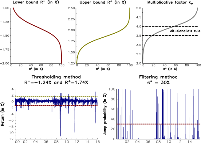
Figure 19: Detecting the jumps of the carry risk premium (weekly model)

To show the equivalence of the two approaches, we consider the returns $R_{t}$ of the carry risk premium. Using the weekly model, we calculate the truncation points of the thresholding approach. Results are given in top panels in Figure 19. For instance, when $\pi^{\star}$ is equal to $30\%$, we obtain $R^{-}=-1.24\%$ and $R^{+}=1.74\%$. Therefore, we believe that we have a jump when the weekly return is lower than $-1.24\%$ or when it is higher than $1.74\%$. In the bottom/left panel, we illustrate the thresholding approach with $R^{-}=-1.24\%$ and $R^{+}=1.74\%$ whereas the filtering approach is showed in the bottom/right panel with $\pi^{\star}=30\%$. As expected, the two approaches detect the jumps at the same times.

A.8 Derivation of the thresholding approach in the multi-dimensional case

We use the following parametrization of the probability density function:

$$f\left(y\right)=\left(1-\pi\right)\phi_{n}\left(y_{t},\mu_{1},\Sigma_{1}\right)+\pi\phi_{n}\left(y_{t},\mu_{2},\Sigma_{2}\right)$$

The posteriori probability to have a jump at time $t$ is:

$$\hat{\pi}_{t}=\frac{\pi\phi_{n}\left(y_{t},\mu_{2},\Sigma_{2}\right)}{\left(1-\pi\right)\phi_{n}\left(y_{t},\mu_{1},\Sigma_{1}\right)+\pi\phi_{n}\left(y_{t},\mu_{2},\Sigma_{2}\right)}$$

It follows that $\hat{\pi}_{t}\geq\pi^{\star}$ is equivalent to:

$$\left(y_{t}-\mu_{1}\right)^{\top}\Sigma_{1}^{-1}\left(y_{t}-\mu_{1}\right)-\left(y_{t}-\mu_{2}\right)^{\top}\Sigma_{2}^{-1}\left(y_{t}-\mu_{2}\right)+2\ln\frac{\pi\left(1-\pi^{\ast}\right)}{\pi^{\ast}\left(1-\pi\right)}+\ln\frac{\left|\Sigma_{1}\right|}{\left|\Sigma_{2}\right|}\geq 0$$

We deduce:

$$y_{t}^{\top}\left(\Sigma_{1}^{-1}-\Sigma_{2}^{-1}\right)y_{t}+2\left(\mu_{2}^{\top}\Sigma_{2}^{-1}-\mu_{1}^{\top}\Sigma_{1}^{-1}\right)y_{t}+$$

$$\left(\mu_{1}^{\top}\Sigma_{1}^{-1}\mu_{1}-\mu_{2}^{\top}\Sigma_{2}^{-1}\mu_{2}\right)+2\ln\frac{\pi\left(1-\pi^{\ast}\right)}{\pi^{\ast}\left(1-\pi\right)}+\ln\frac{\left|\Sigma_{1}\right|}{\left|\Sigma_{2}\right|}\geq 0$$

The quadratic form of this inequality is:

$$\left(y_{t}-v\right)^{\top}Q\left(y_{t}-v\right)\geq r^{\star}$$

where:

$$Q = \Sigma_{1}^{-1}-\Sigma_{2}^{-1}$$

$$v = Q^{-1}\left(\Sigma_{1}^{-1}\mu_{1}-\Sigma_{2}^{-1}\mu_{2}\right)$$

$$r^{\star} = v^{\top}Qv+\mu_{2}^{\top}\Sigma_{2}^{-1}\mu_{2}-\mu_{1}^{\top}\Sigma_{1}^{-1}\mu_{1}-2\ln\frac{\pi\left(1-\pi^{\ast}\right)}{\pi^{\ast}\left(1-\pi\right)}-\ln\frac{\left|\Sigma_{1}\right|}{\left|\Sigma_{2}\right|}$$

With the parametrization $\mu_{1}=\mu\,\mathrm{d}t$, $\Sigma_{1}=\Sigma\,\mathrm{d}t$, $\mu_{2}=\mu\,\mathrm{d}t+\tilde{\mu}$ and $\Sigma_{2}=\Sigma\,\mathrm{d}t+\tilde{\Sigma}$, we obtain:

$$Q = \left(\Sigma\,\mathrm{d}t+\tilde{\Sigma}\right)^{-1}\tilde{\Sigma}\left(\Sigma\,\mathrm{d}t\right)^{-1}$$

$$v = \left(\mu-\Sigma\tilde{\Sigma}^{-1}\tilde{\mu}\right)\mathrm{d}t$$

$$r^{\star} = \tilde{\mu}^{\top}\tilde{\Sigma}^{-1}\tilde{\mu}-2\ln\frac{\pi\left(1-\pi^{\ast}\right)}{\pi^{\ast}\left(1-\pi\right)}-\ln\frac{\left|\Sigma\,\mathrm{d}t\right|}{\left|\Sigma\,\mathrm{d}t+\tilde{\Sigma}\right|}$$

The solution of the quadratic equation $\left(y_{t}-v\right)^{\top}Q\left(y_{t}-v\right)=r^{\star}$ is a $n$-dimensional ellipsoid centered at $v$ and whose semi-axes are the square root of the eigenvalues of the matrix $r^{\star}Q^{-1}$. We deduce that the solution is not unique and can not be expressed in terms of truncation points:

$$J_{t}=1\nLeftrightarrow y_{i,t}\leq y_{i}^{-}\text{ and }y_{i,t}\geq y_{i}^{+}$$

We consider again the equity/bond/volatility example. In the top panel in Figure 20, we report the solution of the quadratic equation, which is an ellipsoid. For the thresholding method, we compare at each date the quadratic form $\mathbb{QF}_{t}=\left(R_{t}-v\right)^{\top}Q\left(R_{t}-v\right)$ with the threshold $r^{\star}=16.03$ calculated using the numerical values of Table 9. We will say that we observe a jump if the following conditions holds:

$$J_{t}=1\Leftrightarrow\mathbb{QF}_{t}\geq r^{\star}$$

The filtering method is given in the bottom/right panel. In this case, we have:

$$J_{t}=1\Leftrightarrow\pi_{t}\geq\pi^{\star}$$

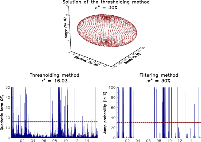
Figure 20: Detecting the jumps in the multivariate case (weekly model)

A.9 Filtering algorithm for estimating $\hat{\mu}_{t}$ and $\hat{\Sigma}_{t}$

We consider a sample $\left\{y_{1},\ldots,y_{T}\right\}$ of $T$ observations. We note $y_{i,t}$ the value of the $i^{\mathrm{th}}$ component at time $t$. Given $\pi$, $\tilde{\mu}$ and $\tilde{\Sigma}$, we would like to estimate the parameters $\hat{\mu}_{t}$ and $\hat{\Sigma}_{t}$ by assuming that the probability density function of the mixture model is:

$$f\left(y\right)=\left(1-\pi\right)\phi_{n}\left(y;\mu\,\mathrm{d}t,\Sigma\,\mathrm{d}t\right)+\pi\phi_{n}\left(y;\mu\,\mathrm{d}t+\tilde{\mu},\Sigma\,\mathrm{d}t+\tilde{\Sigma}\right)$$

We assume that there is a jump at time $t$ if the filtering probability $\hat{\pi}_{t}$ is larger than a given threshold $\pi^{\star}$:

$$J_{t}=1\Leftrightarrow\hat{\pi}_{t}\geq\pi^{\star}$$

The algorithm for estimating the parameters is then given by the following steps:

1. Let $n_{rw}$ be the length of the rolling window. We initialize the filtering procedure at time $n_{rw}+1$.

2. At time $t$, we calculate the posterior jump probabilities:

   $$\hat{\pi}_{t-s}=\frac{\pi\phi_{n}\left(y_{t-s},\hat{\mu}_{t-1}\,\mathrm{d}t+\tilde{\mu},\hat{\Sigma}_{t-1}\,\mathrm{d}t+\tilde{\Sigma}\right)}{\left(1-\pi\right)\phi_{n}\left(y_{t-s},\hat{\mu}_{t-1}\,\mathrm{d}t,\hat{\Sigma}_{t-1}\,\mathrm{d}t\right)+\pi\phi_{n}\left(y_{t-s},\hat{\mu}_{t-1}\,\mathrm{d}t+\tilde{\mu},\hat{\Sigma}_{t-1}\,\mathrm{d}t+\tilde{\Sigma}\right)}$$

   for $s=0,\ldots,n_{rw}-1$. The probabilities $\hat{\pi}_{t-s}$ are based on the estimates $\hat{\mu}_{t-1}$ and $\hat{\Sigma}_{t-1}$ calculated at time $t-1$.

3. We update the estimates $\hat{\mu}_{t-1}$ and $\hat{\Sigma}_{t-1}$ using the following formulas:

   $$\hat{\mu}_{i,t}\,\mathrm{d}t=\frac{1}{n_{t}}\sum_{s=0}^{n_{rw}-1}\mathds{1}\left\{\hat{\pi}_{t-s}\leq\bar{\pi}\right\}\cdot y_{i,t-s}$$

   $$\hat{\Sigma}_{i,j,t}\,\mathrm{d}t=\frac{1}{n_{t}}\sum_{s=0}^{n_{rw}-1}\mathds{1}\left\{\hat{\pi}_{t-s}\leq\bar{\pi}\right\}\cdot\left(y_{i,t-s}-\hat{\mu}_{i,t}\right)\left(y_{j,t-s}-\hat{\mu}_{j,t}\right)$$

   where $n_{t}$ indicates the number of observations that do not jump:

   $$n_{t}=\sum_{s=0}^{n_{rw}-1}\mathds{1}\left\{\hat{\pi}_{t-s}\leq\bar{\pi}\right\}$$

   These new estimates $\hat{\mu}_{t}$ and $\hat{\Sigma}_{t}$ will be valid to calculate the posterior probabilities $\hat{\pi}_{t+1-s}$.

4. We go back to Step 2.

To initialize the algorithm, we can use the traditional Gaussian estimates.

Appendix B Additional results

Table 12: Estimation of the Gaussian model (weekly model)

Asset	$\mu_{i}$	$\sigma_{i}$	$\rho_{i,j}$
Bonds	$5.38$	${\hskip 5.0pt}4.17$	${\hskip 3.0pt}100.00$
Equities	$6.09$	$18.38$	$-34.43$	$100.00$
Carry	$6.00$	${\hskip 5.0pt}5.50$	$-18.22$	${\hskip 5.0pt}51.92$	$100.00$

Table 13: Estimation of the Gaussian model (monthly model)

Asset	$\mu_{i}$	$\sigma_{i}$	$\rho_{i,j}$
Bonds	$5.32$	${\hskip 5.0pt}4.31$	${\hskip 3.0pt}100.00$
Equities	$5.91$	$16.97$	$-28.56$	$100.00$
Carry	$6.26$	${\hskip 5.0pt}6.91$	$-14.50$	${\hskip 5.0pt}55.21$	$100.00$

Table 14: Estimation of the Gaussian model (annually model)

Asset	$\mu_{i}$	$\sigma_{i}$	$\rho_{i,j}$
Bonds	$5.29$	${\hskip 5.0pt}4.03$	${\hskip 3.0pt}100.00$
Equities	$6.47$	$18.59$	$-69.26$	$100.00$
Carry	$6.68$	${\hskip 5.0pt}8.16$	$-26.22$	${\hskip 5.0pt}63.25$	$100.00$

Table 15: Estimation of the Gaussian mixture model when $\pi=5\%$ (weekly model)

Asset	$\mu_{i}$	$\sigma_{i}$	$\rho_{i,j}$
Bonds	${\hskip 8.0pt}4.65$	${\hskip 5.0pt}3.84$	${\hskip 3.0pt}100.00$
Equities	${\hskip 3.0pt}10.85$	$14.32$	$-34.78$	$100.00$
Carry	${\hskip 3.0pt}11.35$	${\hskip 5.0pt}2.53$	$-22.40$	${\hskip 5.0pt}57.72$	$100.00$
Asset	$\tilde{\mu}_{i}$	$\tilde{\sigma}_{i}$	$\tilde{\rho}_{i,j}$
Bonds	${\hskip 8.0pt}0.18$	${\hskip 5.0pt}0.78$	${\hskip 3.0pt}100.00$
Equities	$-1.26$	${\hskip 5.0pt}5.56$	$-35.80$	$100.00$
Carry	$-1.30$	${\hskip 5.0pt}2.04$	$-16.34$	${\hskip 5.0pt}53.86$	$100.00$

Table 16: Estimation of the Gaussian mixture model when $\pi=5\%$ (monthly model)

Asset	$\mu_{i}$	$\sigma_{i}$	$\rho_{i,j}$
Bonds	${\hskip 8.0pt}4.25$	${\hskip 5.0pt}4.01$	${\hskip 3.0pt}100.00$
Equities	${\hskip 3.0pt}10.76$	$13.79$	$-33.04$	$100.00$
Carry	${\hskip 3.0pt}10.14$	${\hskip 5.0pt}2.61$	$-19.03$	${\hskip 5.0pt}46.49$	$100.00$
Asset	$\tilde{\mu}_{i}$	$\tilde{\sigma}_{i}$	$\tilde{\rho}_{i,j}$
Bonds	${\hskip 8.0pt}1.18$	${\hskip 5.0pt}1.21$	${\hskip 3.0pt}100.00$
Equities	$-5.33$	${\hskip 5.0pt}8.97$	${\hskip 8.0pt}26.78$	$100.00$
Carry	$-4.14$	${\hskip 5.0pt}5.21$	${\hskip 8.0pt}32.51$	${\hskip 5.0pt}65.69$	$100.00$

Table 17: Estimation of the Gaussian mixture model when $\pi=1\%$ (weekly model)

Asset	$\mu_{i}$	$\sigma_{i}$	$\rho_{i,j}$
Bonds	${\hskip 8.0pt}4.75$	${\hskip 5.0pt}3.95$	${\hskip 3.0pt}100.00$
Equities	${\hskip 8.0pt}9.23$	$15.21$	$-34.60$	$100.00$
Carry	${\hskip 3.0pt}10.51$	${\hskip 5.0pt}2.80$	$-22.91$	${\hskip 5.0pt}56.83$	$100.00$
Asset	$\tilde{\mu}_{i}$	$\tilde{\sigma}_{i}$	$\tilde{\rho}_{i,j}$
Bonds	${\hskip 8.0pt}0.29$	${\hskip 5.0pt}0.85$	${\hskip 3.0pt}100.00$
Equities	$-1.56$	${\hskip 5.0pt}6.66$	$-35.97$	$100.00$
Carry	$-1.98$	${\hskip 5.0pt}2.43$	$-7.65$	${\hskip 5.0pt}57.45$	$100.00$

Table 18: Estimation of the Gaussian mixture model when $\pi=1\%$ (monthly model)

Asset	$\mu_{i}$	$\sigma_{i}$	$\rho_{i,j}$
Bonds	${\hskip 8.0pt}4.57$	${\hskip 5.0pt}4.07$	${\hskip 3.0pt}100.00$
Equities	${\hskip 8.0pt}9.16$	$14.54$	$-32.14$	$100.00$
Carry	${\hskip 8.0pt}9.70$	${\hskip 5.0pt}2.90$	$-19.56$	${\hskip 5.0pt}47.68$	$100.00$
Asset	$\tilde{\mu}_{i}$	$\tilde{\sigma}_{i}$	$\tilde{\rho}_{i,j}$
Bonds	${\hskip 8.0pt}1.36$	${\hskip 5.0pt}1.33$	${\hskip 3.0pt}100.00$
Equities	$-5.84$	$10.17$	${\hskip 3.0pt}30.97$	$100.00$
Carry	$-5.94$	${\hskip 5.0pt}5.77$	${\hskip 3.0pt}55.18$	${\hskip 5.0pt}74.83$	$100.00$

Table 19: Estimation of the Gaussian mixture model when $\lambda=10\%$ (weekly model)

Asset	$\mu_{i}$	$\sigma_{i}$	$\rho_{i,j}$
Bonds	${\hskip 8.0pt}4.85$	${\hskip 5.0pt}3.99$	${\hskip 3.0pt}100.00$
Equities	${\hskip 8.0pt}8.53$	$15.70$	$-35.21$	$100.00$
Carry	${\hskip 3.0pt}10.10$	${\hskip 5.0pt}2.94$	$-23.44$	${\hskip 5.0pt}56.95$	$100.00$
Asset	$\tilde{\mu}_{i}$	$\tilde{\sigma}_{i}$	$\tilde{\rho}_{i,j}$
Bonds	${\hskip 8.0pt}0.33$	${\hskip 5.0pt}0.89$	${\hskip 3.0pt}100.00$
Equities	$-1.71$	${\hskip 5.0pt}7.22$	$-32.16$	$100.00$
Carry	$-2.46$	${\hskip 5.0pt}2.62$	$-1.96$	${\hskip 5.0pt}60.59$	$100.00$

Table 20: Estimation of the Gaussian mixture model when $\lambda=10\%$ (monthly model)

Asset	$\mu_{i}$	$\sigma_{i}$	$\rho_{i,j}$
Bonds	${\hskip 8.0pt}4.59$	${\hskip 5.0pt}4.08$	${\hskip 3.0pt}100.00$
Equities	${\hskip 8.0pt}8.96$	$14.64$	$-31.97$	$100.00$
Carry	${\hskip 8.0pt}9.64$	${\hskip 5.0pt}2.93$	$-19.58$	${\hskip 5.0pt}48.02$	$100.00$
Asset	$\tilde{\mu}_{i}$	$\tilde{\sigma}_{i}$	$\tilde{\rho}_{i,j}$
Bonds	${\hskip 8.0pt}1.38$	${\hskip 5.0pt}1.34$	${\hskip 3.0pt}100.00$
Equities	$-5.79$	$10.28$	${\hskip 3.0pt}30.71$	$100.00$
Carry	$-6.15$	${\hskip 5.0pt}5.83$	${\hskip 3.0pt}58.45$	${\hskip 5.0pt}76.92$	$100.00$

Table 21: Estimation of the constrained mixture model when $\pi=1\%$ (monthly model)

Asset	$\mu_{i}$	$\sigma_{i}$	$\rho_{i,j}$
Bonds	${\hskip 8.0pt}5.32$	${\hskip 5.0pt}4.31$	${\hskip 3.0pt}100.00$
Equities	${\hskip 8.0pt}8.69$	$14.53$	$-32.57$	$100.00$
Carry	${\hskip 8.0pt}9.54$	${\hskip 5.0pt}2.94$	$-22.21$	${\hskip 5.0pt}48.50$	$100.00$
Asset	$\tilde{\mu}_{i}$	$\tilde{\sigma}_{i}$	$\tilde{\rho}_{i,j}$
Bonds	${\hskip 8.0pt}0.00$	${\hskip 5.0pt}0.00$	$100.00$
Equities	$-5.46$	$10.86$	${\hskip 10.0pt}0.00$	$100.00$
Carry	$-6.16$	${\hskip 5.0pt}5.93$	${\hskip 10.0pt}0.00$	${\hskip 5.0pt}73.28$	$100.00$

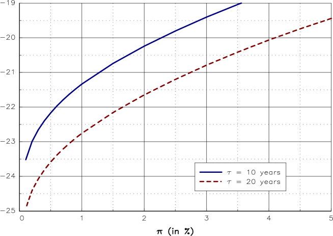
Figure 21: Expected monthly drawdown (in %) of the carry risk premium

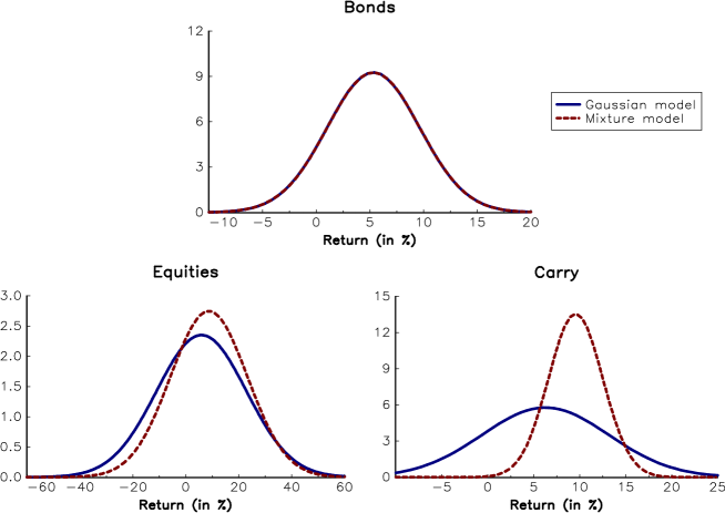
Figure 22: Probability density function of asset returns in the normal regime (monthly model)

References

- [1] Acerbi, C., and Tasche, D. (2002), On the Coherence of Expected Shortfall, Journal of Banking & Finance, 26(7), pp. 1487-1503.
- [2] Ait-Sahalia, Y. (2004), Disentangling Diffusion from Jumps, Journal of Financial Economics, 74(3), pp. 487-528.
- [3] Aït-Sahalia, Y., and Jacod, J. (2012), Analyzing the Spectrum of Asset Returns: Jump and Volatility Components in High Frequency Data, Journal of Economic Literature, 50(4), pp. 1007-1050.
- [4] Ang, A. (2014), Asset Management – A Systematic Approach to Factor Investing, Oxford University Press.
- [5] Billio, M., Getmansky, M., and Pelizzon, L. (2012), Dynamic Risk Exposures in Hedge Funds, Computational Statistics & Data Analysis, 56(11), pp. 3517-3532.
- [6] Cazalet, Z., and Roncalli, T. (2014), Facts and Fantasies About Factor Investing, SSRN, www.ssrn.com/abstract=2524547.
- [7] Daniel, K.D., and Moskowitz, T.J. (2016), Momentum Crashes, Jorunal of Financial Economics, forthcoming.
- [8] Dempster, A.P., Laird, N.M., and Rubin, D.B. (1977), Maximum Likelihood from Incomplete Data via the EM Algorithm, Journal of the Royal Statistical Society, B39(1), pp. 1-38.
- [9] Eraker, B., Johannes, M., and Polson, N. (2003), The Impact of Jumps in Volatility and Returns, Journal of Finance, 58(3), pp. 1269-1300.
- [10] Hamdan, R., Pavlowsky, F., Roncalli, T. and Zheng, B. (2016), A Primer on Alternative Risk Premia, SSRN, www.ssrn.com/abstract=2766850.
- [11] Hamilton, J.D. (1989), A New Approach to the Economic Analysis of Nonstationary Time Series and the Business Cycle, Econometrica, 57(2), pp. 357-384.
- [12] Harvey, C.R., and Siddique, A. (2000), Conditional Skewness in Asset Pricing Tests, Journal of Finance, 55(3), pp. 1263-1295.
- [13] Jondeau, E., and Rockinger, M. (2006), Optimal Portfolio Allocation under Higher Moments, European Financial Management, 12(1), pp. 29-55.
- [14] Jurczenko, E., and Maillet, B. (2006), Multi-moment Asset Allocation and Pricing Models, John Wiley & Sons.
- [15] Kraus, A., and Litzenberger, R.H. (1976), Skewness Preference and the Valuation of Risk Assets, Journal of Finance, 31(4), pp. 1085-1100.
- [16] Lempérière, Y., Deremble, C., Nguyen, T.T., Seager, P., Potters, M., and Bouchaud, J-P. (2014), Risk Premia: Asymmetric Tail Risks and Excess Returns, SSRN, www.ssrn.com/abstract=2502743.
- [17] Maeso, J-M., and Martellini, L. (2016), Factor Investing and Risk Allocation: From Traditional to Alternative Risk Premia Harvesting, EDHEC Working Paper.
- [18] Maillard, S., Roncalli, T. and Teïletche, J. (2010), The Properties of Equally Weighted Risk Contribution Portfolios, Journal of Portfolio Management, 36(4), pp. 60-70.
- [19] Martellini, L. and Ziemann, V. (2010), Improved Estimates of Higher-Order Comoments and Implications for Portfolio Selection, Review of Financial Studies, 23(4), pp. 1467-1502.
- [20] Pan, J. (2002), The Jump-risk Premia Implicit in Options: Evidence from an Integrated Time-series Study, Journal of Financial Economics, 63(1), pp. 3-50.
- [21] Patton, A.J. (2004), On the Out-of-sample Importance of Skewness and Asymmetric Dependence for Asset Allocation, Journal of Financial Econometrics, 2(1), pp. 130-168.
- [22] Redner, R.A., and Walker, H.F. (1984), Mixture Densities, Maximum Likelihood and the EM Algorithm, SIAM Review, 26(2), pp. 195-239.
- [23] Roncalli, T. (2013), Introduction to Risk Parity and Budgeting, Chapman & Hall/CRC Financial Mathematics Series.
- [24] Roncalli, T. (2015), Introducing Expected Returns into Risk Parity Portfolios: A New Framework for Asset Allocation, Bankers, Markets & Investors, 138, pp. 18-28.
- [25] Roncalli, T., and weisang, G. (2016), Risk Parity Portfolios with Risk factors, Quantitative Finance, 16(3), pp. 377-388.
- [26] Spinu, F. (2013), An Algorithm for the Computation of Risk Parity Weights, SSRN, www.ssrn.com/abstract=2297383.
- [27] Xiong, J.X., and Idzorek, T.M. (2011), The Impact of Skewness and Fat Tails on the Asset Allocation Decision, Financial Analysts Journal, 67(2), pp. 23-35.
- [28] Xu, L., and Jordan, M.I. (1996), On Convergence Properties of the EM Algorithm for Gaussian Mixtures, Neural Computation, 8(1), pp. 129-151.