Extraction of interaction parameters for $\alpha$-RuCl₃ from neutron data using machine learning

Abstract

Single crystal inelastic neutron scattering data contain rich information about the structure and dynamics of a material. Yet the challenge of matching sophisticated theoretical models with large data volumes is compounded by computational complexity and the ill-posed nature of the inverse scattering problem. Here we utilize a novel machine-learning-assisted framework featuring multiple neural network architectures to address this via high-dimensional modeling and numerical methods. A comprehensive data set of diffraction and inelastic neutron scattering measured on the Kitaev material $\alpha-$RuCl₃ is processed to extract its Hamiltonian. Semiclassical Landau-Lifshitz dynamics and Monte-Carlo simulations were employed to explore the parameter space of an extended Kitaev-Heisenberg Hamiltonian. A machine-learning-assisted iterative algorithm was developed to map the uncertainty manifold to match experimental data; a non-linear autoencoder used to undertake information compression; and Radial Basis networks utilized as fast surrogates for diffraction and dynamics simulations to predict potential spin Hamiltonians with uncertainty. Exact diagonalization calculations were employed to assess the impact of quantum fluctuations on the selected parameters around the best prediction.

Introduction.—Highly frustrated quantum systems are important routes to realizing exotic ground states and excitations. They are proposed to host states ranging from long-range entangled quantum spin liquids (QSLs) with nonlocal excitations to quantum spin ices with emergent photons [1, 2, 3]. Recently, the two-dimensional honeycomb spin-1/2 material $\alpha$-RuCl₃ [Fig. 1(a)] has garnered particular attention following being reported [4, 5, 6, 7, 8, 9, 10, 11] as a leading candidate [12, 13, 14] for realization of the Kitaev model—an exactly solvable QSL Hamiltonian [15, 16]. The Kitaev model is a spin network with competing bond-dependent interactions and hosts a topological QSL ground state that supports two types of fractionalized excitations: visons, which are excitations of the emergent flux, and deconfined Majorana fermions. These quasiparticles are predicted to show non-Abelian statistics, suggesting potential applications in e.g. topological quantum computing [17]. Recently, theoretical propositions have been made for interferometers utilizing their braiding statistics as a precursor to undertaking quantum operations [18, 19]. Meanwhile, however, the experimental situation regarding the quasiparticles in $\alpha$-RuCl₃ remains inconclusive, primarily due to difficulties in determining the precise nature of the spin couplings in the material and to what extent these destabilize the QSL state in zero and applied magnetic fields.

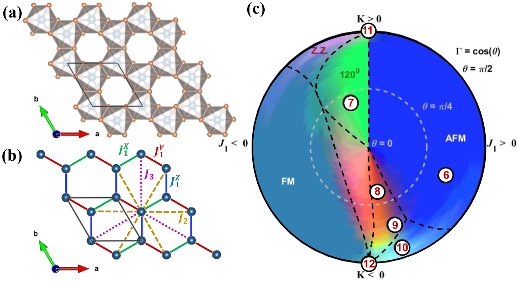
Figure 1: (a) $\alpha$-RuCl₃ crystal structure, consisting of Ru sites at centers of edge-sharing Cl octahedra. (b) The magnetism is due to Ru³⁺ ions, which form a honeycomb lattice. Nearest, second-nearest, and third-nearest neighbor bonds are indicated by solid, dashed, and dotted lines respectively. Anisotropic nearest-neighbor interactions are considered as given in Eq. (1). (c) Machine-learned phase diagram for the $J_{1}-K-\Gamma$ model at $T=1$ K, with theoretical phase boundaries from Ref. [20] overlaid in black dashed lines. The different colors, which represent different structure factors $S(\textbf{Q})$, are predicted by a trained neural network as explained in the main text. Numbered points correspond to $S(\textbf{Q})$ shown in Fig. 2(b). The identified phases include ferromagnetic [FM], Néel [AFM], $120^{\degree}$, and zigzag [Z.Z.] orders.

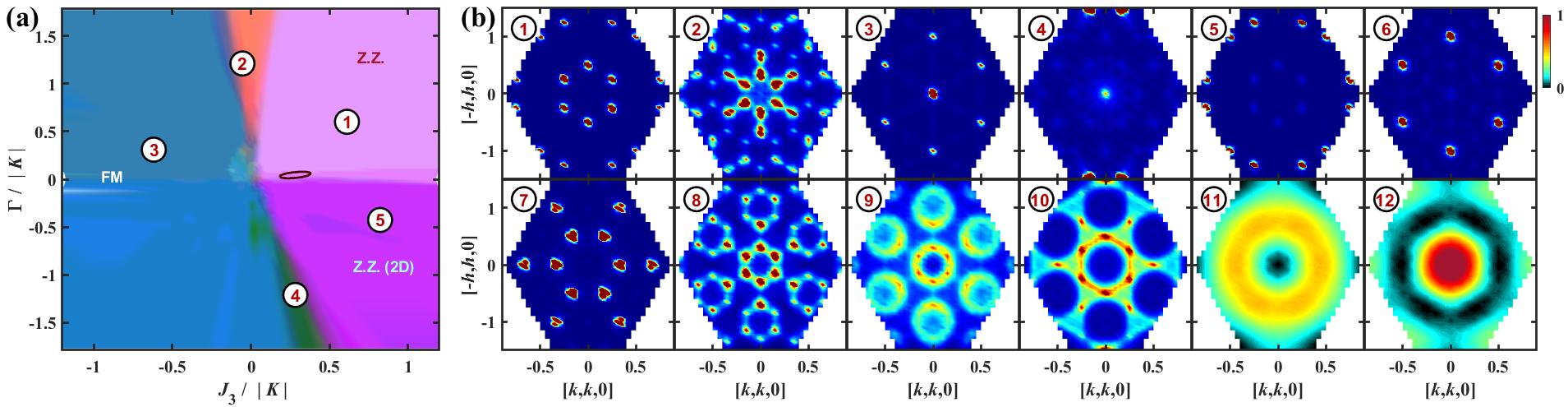
Figure 2: (a) Machine-learned phase map varying $\Gamma/|K|$ and $J_{3}/|K|$ through the optimal solution for $\alpha$-RuCl₃ at fixed $J_{1}/|K|=-0.1$ and $J_{2}/|K|=0$, with $K<0$. Labeled phases include ferromagnetic [FM], zigzag [Z.Z.] and planar zigzag [Z.Z. (2D)] orders. The ellipsoidal approximation to the optimal solution is marked in panel (a) in dark-red. Due to uneven sampling of the IMA process from which the data was taken, the prediction accuracy varies in parameter space resulting in a blotchy appearance. The different colors, which represent different structure factors $S(\textbf{Q})$, are predicted by a trained neural network as explained in the main text. Panel (b) shows the surrogate predicted neutron structure factor, $S^{\rm Sur}(\textbf{Q}),$ at numbered locations indicated in (a) and Fig. 1(c). Corresponding spin structures for the long-range ordered phases labeled 1, 3-7 are given in the SM [21]. Note that Z.Z. and Z.Z. (2D) have similar long-range order, but along different spin-orientation directions. This occurs because, as discussed in Ref. [22], when $K<0$ the spin orientation in zigzag ground states depends on the sign of $\Gamma$. Due to the neutron spin polarization factor, the two $S(\textbf{Q})$ are different in the shown plane, despite yielding the same trace over spin correlations, $\sum_{\alpha}S^{\alpha\alpha}\left(\mathbf{Q}\right)$. Some of the diffuse $S(\textbf{Q})$, taken at either phase boundaries or critical points, are also shown. The $S(\textbf{Q})$ labeled 11 and 12 are for the pure AFM and FM Kitaev models.

Experiments have revealed evidence that $\alpha$-RuCl₃ is close to the Kitaev QSL [12, 13, 23, 24]. At low temperatures and magnetic fields it orders magnetically in a zigzag structure [25, 26, 27, 6], implying the presence of symmetry-allowed interactions additional to the Kitaev Hamiltonian, as is generically predicted by theory [28, 20, 29, 30]. Inelastic neutron scattering (INS) shows scattering dominated by continua at the zone center [7, 8, 9, 10, 11], interpreted as originating from underlying fractional Majorana excitations, or from incoherent excitations due to magnon decay [31, 32, 33]; both related to strongly fluctuating quantum states. Similarly, Raman scattering shows a broad scattering continuum at the zone center [5, 34, 35, 36, 37], and a fermionic temperature dependence, interpreted as indicating fractional excitations. The zigzag order melts in a narrow range of applied in-plane magnetic fields, possibly inducing a QSL state [10, 11, 38, 39, 40]. Oscillations of the thermal conductivity were also observed in this field range, suggesting the presence of a Fermi surface [41, 42, 43]. Perhaps the most striking reports are those of a half-integer-quantized thermal Hall effect in the same field range [44, 45, 46]. Additional experimental evidence for Kitaev interactions in $\alpha$-RuCl₃ has been reported using e.g. inelastic X-ray scattering [47], thermodynamical [48, 8, 49, 50, 51], NMR [39, 52], electron spin resonance [53], microwave absorption [54], thermal transport [55, 56], and THz spectroscopy [57, 58, 59, 60, 61] techniques.

The complexity of magnetic interactions in RuCl₃ has hindered determination of an underlying model. Various groups have fit or derived proposed Hamiltonian parameters for the material [29, 31, 62, 59, 63, 64, 65, 66, 67, 68, 69, 30, 9, 6, 60, 23, 70, 24, 71], but these studies disagree significantly about which interactions are present, and on values of specific interaction parameters [72, 73, 33]. Part of the reason for this lack of agreement is that many experimental fits have relied on linear spin wave theory (LSWT), which cannot account for the quantum fluctuations inherent to $\alpha$-RuCl₃. However, the more central issue is that a comparatively large set of weak perturbations are possible, that can significantly modify the magnetic ordering, dynamics and thermal properties of Kitaev materials. With such a high-dimensional parameter space, comparing modeling with experimental data leaves a great deal of uncertainty, unless comprehensive enough to explore the range of possible interactions; an approach which is absent to date.

Scattering data contain considerable information on the magnetic states and interactions in materials. A difficult step in the quantification of models has been inversion from measured data to a model—the so-called inverse scattering problem, which is usually ill-posed due to loss of phase information. In this regard, machine learning (ML) [74, 75] has shown promising results [76, 77, 78, 79, 80]. Here we combine ML approaches with large-scale semi-classical simulations (SCSs) [80]. ML-SCS techniques have been used to successfully extract couplings from diffuse neutron scattering data and yielded significant insight by mapping the physical behavior in high-dimensional interaction spaces of materials [81, 80]. We extend these methods to include dynamics data for $\alpha$-RuCl₃, allowing a comprehensive fit.

Experiments.—Elastic neutron studies were performed at the Spallation Neutron Source (SNS) [82] using the CORELLI beamline [83]. A 125 mg $\alpha$-RuCl₃ crystal was mounted on an aluminium plate and aligned with the $[h,0,l]$ plane horizontal. The crystal was rotated through $170$ degrees in $2^{\degree}$ steps about the vertical axis. The temperature of the measurement was 2 K and the perpendicular wave vector transfer was integrated in the range $l$ = [0.92, 1.08] r.l.u.. The elastic scattering data was previously published as Supplementary Figure S2(a) in Ref. [10].

INS was performed on a $0.7$ g single crystal, which was sealed in a thin-walled aluminium can with 1 atmosphere of Helium gas for thermal contact. Measurements at $4$ K were carried out using the SEQUOIA spectrometer [84, 85] at the SNS. The incident energy was set to $E_{i}=22.5$ meV. The crystal was mounted with $[h,0,0]$ and $[0,0,l]$ axes in the horizontal plane, and the orthogonal $[0.5k,-k,0]$ axis pointing vertically upwards. Data were collected by rotating the crystal about the vertical axis over $290^{\degree}$ in $1^{\degree}$ steps. The data are integrated over the range $[0,0,l]$= [-3.5, 3.5].

Modeling.—We consider a generalized spin-$1/2$ Kitaev-Heisenberg spin (local moment) Hamiltonian,

$$H =\sum_{\gamma=X,Y,Z}\sum_{\langle i,j\rangle^{\gamma}}\mathbf{S}_{i}\cdot J_{1}^{\gamma}\cdot\mathbf{S}_{j}$$

$$+J_{2}\sum_{\langle\langle i,j\rangle\rangle}\mathbf{S}_{i}\cdot\mathbf{S}_{j}+J_{3}\sum_{\langle\langle\langle i,j\rangle\rangle\rangle}\mathbf{S}_{i}\cdot\mathbf{S}_{j},$$ (1)

on the honeycomb lattice [Fig. 1(b)], which is expected to capture relevant interactions in the 2D plane. $\langle\dots\rangle$, $\langle\langle\dots\rangle\rangle$, and $\langle\langle\langle\dots\rangle\rangle\rangle$ represent nearest, next-nearest and third-nearest neighbors, respectively, and ${\footnotesize J_{1}^{X}=\begin{bmatrix}J_{1}+K&0&0\\ 0&J_{1}&\Gamma\\ 0&\Gamma&J_{1}\\ \end{bmatrix},J_{1}^{Y}=\begin{bmatrix}J_{1}&0&\Gamma\\ 0&J_{1}+K&0\\ \Gamma&0&J_{1}\\ \end{bmatrix},\\ J_{1}^{Z}=\begin{bmatrix}J_{1}&\Gamma&0\\ \Gamma&J_{1}&0\\ 0&0&J_{1}+K\\ \end{bmatrix}\\ }$
Exchange matrices are defined in the $\{X,Y,Z\}$ coordinate system with principal axes along mutually orthogonal normal vectors of three nearest neighbor Ru-Cl-Ru-Cl plaquettes. Our model includes nearest-neighbor Heisenberg ($J_{1}$), Kitaev ($K$) and symmetric off-diagonal Gamma ($\Gamma$) interactions, as well as second- ($J_{2}$) and third-nearest ($J_{3}$) Heisenberg exchanges. For $J_{2}=0$ it reduces to a proposed minimal model for $\alpha$-RuCl₃ [29]. Eq. (1) is, however, restricted compared to some proposed models, notably neglecting e.g. interlayer exchange [11, 86, 23], and the $\Gamma^{\prime}$ term associated with trigonal distortion [20]. There are conflicting reports as to the magnitude of $\Gamma^{\prime}$ [73, 33, 70], such that neglecting it may not be fully justified. Nevertheless, this choice of Hamiltonian allows us to reduce the computational complexity, and to clearly present our proposed method and its capabilities. We note that ML-SCS techniques have been used to theoretically explore phase diagrams of related Hamiltonians [87, 88].

To simulate spin structure and dynamics, Metropolis (Monte Carlo) sampling [89] and Landau-Lifshitz (LL) dynamics is used [80]. This incorporates effects beyond LSWT, while achieving sufficiently good performance to allow generating a sufficient amount of training data. Spin-$1/2$ operators in Eq. (1) are approximated by classical spin vectors subject to semiclassical normalization, $|\mathbf{S}_{i}|=\sqrt{S(S+1)}$. Metropolis sampling is carried out at fixed temperature, yielding well-thermalized spin configurations. Spin dynamics is governed by the usual LL equations of motion, see Supplemental Material (SM) [21]. The LL equation is solved numerically using a fourth-order Runge-Kutta algorithm with adaptive step size [90]. We use a cluster of 20x20 unit cells (2400 spins) with periodic boundary conditions [21]. Neutron magnetic form factor for Ru³⁺, polarization factors, and instrumental resolution are accounted for, to match with experimental data. Figure 2(b) shows sampling of diffuse scattering at different locations in parameter space. The simulated scattering , $S^{\rm sim}(\textbf{Q})$, shows complex behavior, reflecting the rich physics of Eq. (1).

Machine learning method.—

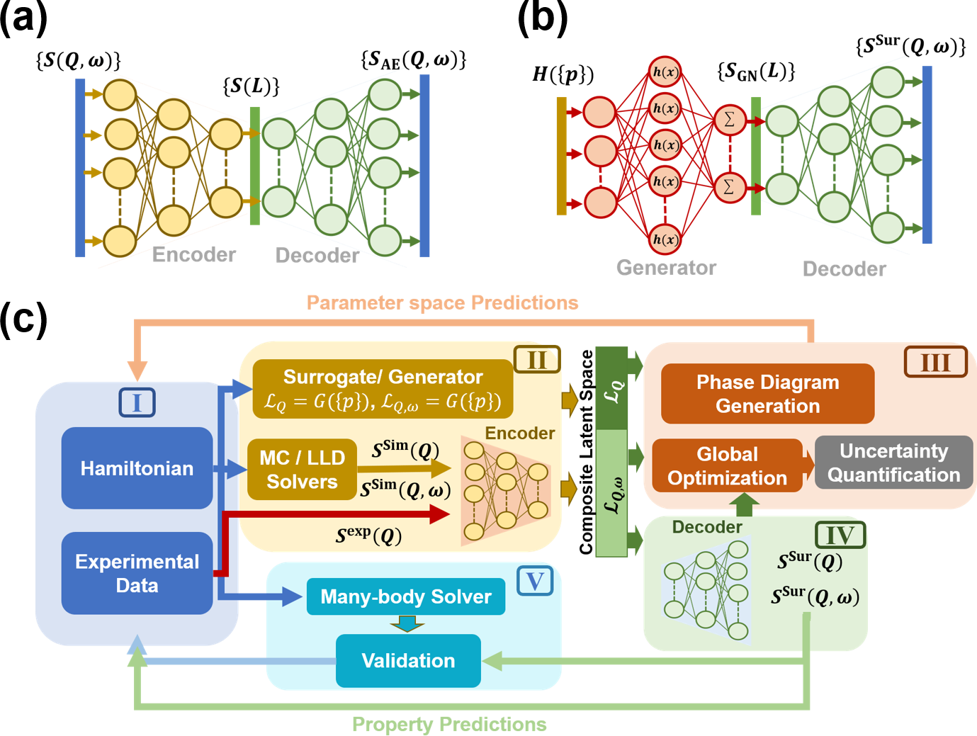
Figure 3: Schematic illustrations of ML methods. (a) Autoencoder architecture used to compress 3D/4D $S(\textbf{Q})$/$S(\textbf{Q},\omega)$ volumes into a much lower dimensionality. The autoencoder is trained with simulated data to reproduce the input. The architecture consists of two networks: Encoder and Decoder. The output of Encoder contains a compressed (latent space) representation, $S(L)$ of the input $S(Q,\omega)$. Decoder decompresses $S(L)$ into a filtered structure factor, $S_{\rm AE}(Q,\omega),$ with the original dimensionality. (b) Schematic design of constructing the surrogate for predicting $S(\textbf{Q})$/$S(\textbf{Q},\omega)$ given a set of model parameters. The surrogate comprises a radial basis network (RBN) as the Generator mapping parameter space, $H(\{p\}),$ to latent space $S_{\rm GN}(L)$ and a Decoder to reconstruct $S(\textbf{Q})$/$S(\textbf{Q},\omega)$ from latent space representations. The generator network (GN) is trained with simulated data for evaluated parameter sets $\{p\}$ as input and corresponding $S(L)$ as target. (c) The ML workflow implemented here to integrate scattering experiments with theory, and extract model parameters and phase-diagram information.

Our method builds on Ref. [81], which recently demonstrated that an ML-integrated method can be used with the experimental static structure factor, $S^{\rm exp}(\textbf{Q}),$ to extract Hamiltonian parameters from diffuse scattering data on a spin ice. Unlike spin ice, $\alpha$-RuCl3 shows a magnetic diffraction pattern with sharp Bragg peaks associated with long-range order, which does not sufficiently constrain the model parameters. Thus we extend the method to account also for the dynamical structure factor, $S^{\rm exp}(Q,\omega)$ from spectroscopy. Although finding a single model to explain the entire 4D scattering is a formidable task, doing so should help avoid fits biased by incomplete information.

A machine-learning-integrated workflow with autoencoder training and global optimization was used to simultaneously fit both $S(\textbf{Q})$ and $S(\textbf{Q},\omega)$. A four-dimensional hyper-parameter space, $\{p\}$, was explored to learn the uncertainty manifold in the five-dimensional parameter space $\{J_{1},K,\Gamma,J_{2},J_{3}\}$ [21] using a variant of the Efficient Global Optimization algorithm [91, 81] which we call the Iterative Mapping algorithm (IMA). Autoencoders are unsupervised artificial neural networks with architecture as shown in Fig. 3(a). We train two autoencoders [21] with either $S(\textbf{Q})$ or $S(\textbf{Q},\omega)$. The Encoder takes a linearized version of the structure factor $S(\nu)$ [$\nu=Q$ or $\nu=Q,\omega$] and outputs a compressed representation, $S(L)$, reducing the input dimensionality $N_{\nu}=10^{6}-10^{8}$ pixels down to $N_{L}=10^{0}-10^{2}$. The Decoder is a contrary network, which projects $S(L)$ back to the original dimensionality and predicts $S_{\rm AE}(\nu)$. Our Encoders and Decoders are designed to be symmetrical, and the numbers of layers are tuned as described in [21].

Two separate Radial Basis Networks (RBN) [92], shown in Fig. 3(b), provide Generator Networks (GN) to approximately map the Hamiltonian space, $H(\{p\})$ directly to latent space, $\mathcal{L}_{\nu}$. See [21] for training details. The GN provides surrogate calculations to bypass the computationally expensive direct solver, allowing exhaustive searches for parameter space mapping as illustrated in Fig. 3(c). GN predictions depend on the degree of training of the network, the topography of the parameter space, and the sampling sparsity. They do not fully replace simulations, and should not be used to draw conclusions when detailed information is needed. Complete surrogates predicting structure factors, $S^{\rm sur}(\nu)$, are constructed by linking the GN with corresponding Decoder. These surrogates can also be used as low-cost estimators in the IMA as an alternative to the Gaussian Process Regression in Ref. [81].

As Fig. 3(c) schematically shows, the workflow can be split into five sections: I) scattering experiment and hypothesis; II) parameter space exploration and information compression; III) structure or property predictions; IV) parameter space predictions; and V) validation of SCS results using a quantum many-body solver. The workflow is similar to one proposed in Ref. [93], but here we add step V and use a composite latent space $\mathcal{L}_{Q}\cup\mathcal{L}_{Q,\omega}$. The latent space forms the backbone of the operation, into which experimental data, simulations, and predictions from GN feed, and from which structure, property, and model parameters are predicted.

ML predictions.—The $S(\textbf{Q})$ (and consequently $S(L)$) provides natural classification of phases, as the correlations of the system are encoded [93]. A high-dimensional graphical phase diagram can be constructed easily by projecting $Q$-space into a latent space of $N_{L}=3$ as suggested in Ref. [93]. An architecture of three intermediate layers with 300-3-300 logistic neurons (activation function as $f(x)=1/(1+e^{-x})$) was empirically found have the highest performance for the $S^{\rm sim}(\textbf{Q})$.

Two phase diagrams are plotted in Figures 1(c) and 2(a). Phases are indicated by color derived by treating latent vectors as RGB color components [80]. Fig. 1(c) corresponds to the $J_{2}=J_{3}=0$ hyperplane, and uses the parametrization [20] $J_{1}=\sin\theta\cos\phi$, $K=\sin\theta\sin\phi$, $\Gamma=\cos\theta$, where the energy scale is fixed according to $1=\sqrt{J_{1}^{2}+K^{2}+\Gamma^{2}}$. Overlaid dashed black lines indicate the theoretically predicted phase diagram. We note that typically our method does not find sharp transitions, so our results are not phase diagrams in a strict sense. Nevertheless, the excellent agreement between Fig. 1(c) and the phase diagram derived in Ref. [20] shows the merit of the approach. Fig. 2(a) shows the phase diagram in a slice around the optimal solution we find for $\alpha$-RuCl₃ (see Fig. 4 and later discussion). Fig. 2(b) indicates the scattering at various points in the two phase diagrams.

To fit experimental scattering data and map uncertainty in the five-dimensional parameter space we employed IMA with cost function ${\hat{\chi}}_{\rm Com}^{2}={\hat{\chi}}_{S(\textbf{Q})}^{2}\times{\hat{\chi}}_{S(Q,\omega)}^{2}$, where the ${\hat{\chi}}_{S(\nu)}^{2}$ are low-cost estimators defined in SM [21]. IMA samples the parameter space iteratively subject to ${\hat{\chi}}_{\rm Com}^{2}\leq C_{\rm Com}$. The threshold value $C_{\rm Com}$ is iteratively reduced to a final value. The Autoencoders and GN, are retrained at the end of each iteration. Thus, the predictability of the networks becomes reliable towards the minimum of ${\hat{\chi}}_{\rm Com}^{2}$.

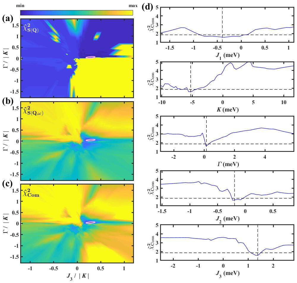
Figure 4: Optimal solution for $\alpha$-RuCl₃. (a) shows a slice of $\hat{\chi}^{2}_{S(\textbf{Q})}$ as function of $J_{3}/|K|$ and $\Gamma/|K|$. The problem is strongly underdetermined when only $S(\textbf{Q})$ is taken into account, with a flat fitness landscape indicating many possible solutions. (b) Same slice for $\hat{\chi}^{2}_{S(Q,\omega)}$. The fitness landscape remains relatively flat when only $S(\mathbf{Q},\omega)$ is accounted for. (c) Slice for the combined $\hat{\chi}^{2}_{\rm Com}$ function, which accounts for both statics and dynamics. An ellipsoidal approximation to the optimal regions is shown in pink on panels (a), (b) and (c). (d) shows line-cuts of $\hat{\chi}^{2}_{\rm Com}$ for individual parameters by fixing other parameters to their optimal values.

Results and Discussion.—Figure 4 shows slices and cuts of the final ${\hat{\chi}}_{\rm Com}^{2}$in parameter space. Due to uncertainties in the data, minimizing ${\hat{\chi}}_{\rm Com}^{2}$ leads to a region of potential fits, indicated by the ellipsoid in panels (a)-(c). Additional Hamiltonian terms may need to be included in the modeling to capture all relevant interactions and achieve higher fitting certainty. This restriction aside, we have identified several parameter sets with particularly low ${\hat{\chi}}_{\rm Com}^{2}$, and these were investigated more closely. Fig. 5 shows $S(\textbf{Q})$ and $S(\textbf{Q},\omega)$ from experiment, LL simulation, and Lanczos exact diagonalization (ED) for the optimized parameter set: $J_{1}=-0.4\pm 0.4$ meV, $K=-5.3\pm 0.3$ meV, $\Gamma=0.15\pm 0.05$ meV, $J_{2}=-0.19\pm 0.15$ meV and $J_{3}=1.35\pm 0.15$ meV. The LL-simulated spectrum shows intensity at both the $M$ and $\Gamma$ points, although the intensity at $\Gamma$ is lower than in the experiment. In addition, the simulation captures the curvature of the spin wave dispersion along the $\Gamma\rightarrow M$ path, as well as the feature at $\omega=6$ meV. ED is subject to finite-size restrictions and low momentum resolution, but captures the magnetic order and energy scale of the low-energy scattering ($\omega<5$ meV).

How does our optimized solution compare to other proposed models for $\alpha$-RuCl₃? Using the surrogates we can easily calculate $\hat{\chi}^{2}$ values for proposed models described by Eq. (1). By this metric our fit outperforms other models in the literature at describing the neutron data, see SM [21]. Our fit has a Kitaev interaction strength comparable to a previous INS fit [31], but lower $\Gamma/K$ and higher $J_{3}/K$. However, the energy scale is generally smaller than for models predicted by band structure calculations, and for models that seek to explain the experimental magnetic specific heat $C(T)$ [73]. Consequently, thermal pure quantum state [94, 95] $C(T)$ results for the optimized solution fail to capture the experimentally observed high-temperature peak [49, 21]. One of our identified near-optimized parameter sets performs better in this regard, but worse at reproducing subtle spectral features [21]. This reinforces the point that Eq. (1) may miss some important term.

One limitation of our approach is the use of SCS. This was necessary to generate large amounts of training data, and allowed us to generate phase diagrams. However, quantum effects can be significant close to phase boundaries, thus locally diminishing the reliability of our networks and requiring many-body verification. This is particularly important in $\alpha$-RuCl₃, which is close to a phase transition under magnetic fields, and where many Hamiltonian parameters matter. Our optimized parameters are close to a transition between the Z.Z. and Z.Z. (2D) orders, but using ED we fortunately find the SCS results are physical, and correctly identifies the ground state. In contrast, the recently proposed Hamiltonian of Ref. [70] is close to a transition between FM and Z.Z. orders, and our SCS predict FM, while ED finds Z.Z. This suggests it may be useful to retrain the networks using many-body simulations in regions close to phase boundaries to increase physical predictability.

Our analysis shows that subtle changes in parameters affect the spectra and ordering. This means that other Hamiltonian terms could also account for the results. This implies that zero field neutron scattering is probably insufficient to constrain the model beyond the treatment here. For a more definitive understanding of $\alpha$-RuCl₃ additional data is needed. Simulations of field dependence suggest that high field spectroscopy measurements should be helpful here in disentangling the contributions of competing terms. Neutron scattering with its ability to capture wavevector and energy effects would be particularly valuable. Co-analysis of high field data along with zero field measurements used here, as well as other observable properties, can then be undertaken using the machine-learning-based approach.

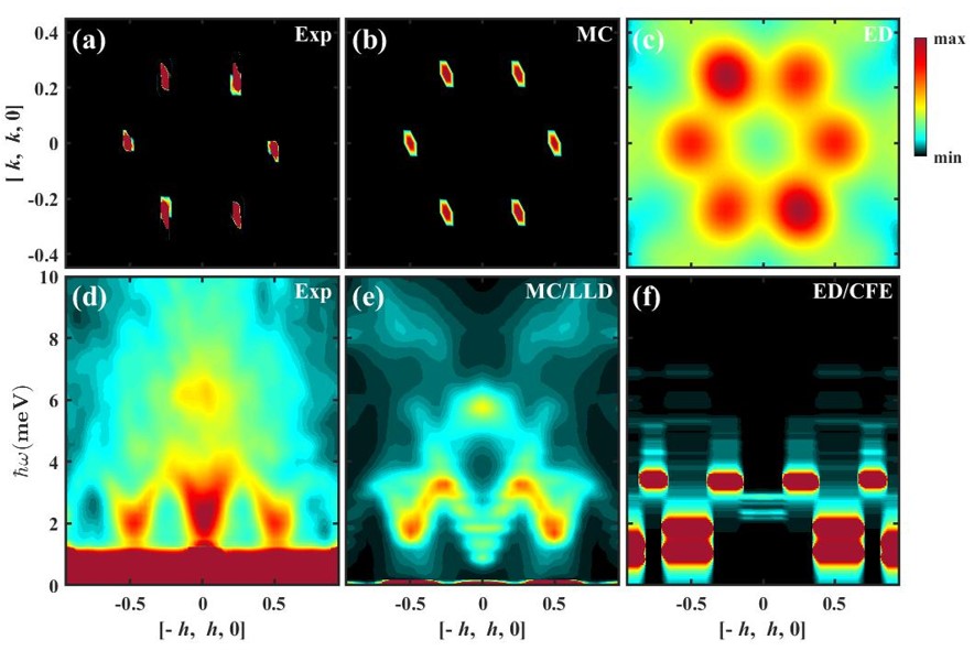
Figure 5: Top row: (a) Experimental and (b,c) theoretical static spin structure factors calculated using (b) MC simulation and (c) Lanczos ED for the optimized Hamiltonian parameters. All methods find peaks at the $M$ points, reflecting the zigzag ordering. Bottom row: Inelastic scattering from (d) experiment, (e) LLD, and (f) Lanczos for the same parameter set.

Conclusion.—We have demonstrated unsupervised ML-SCS methods can be used to solve the inverse scattering problem inherent to INS experiments, thereby extending previous methods to also account for dynamics. Our approach can be applied to a wide range of magnetic systems, to obtain phase diagrams and fit the full 4D experimental scattering, as long as sufficient amounts of training data can be generated. For $\alpha$-RuCl₃ we find a relatively flat fitness landscape, producing an uncertain fit. It does not fully explain the experimental scattering, likely due to interactions not considered here. Nevertheless, the optimal parameters reproduce many smaller scattering features, not captured by other proposed models. Improved algorithms are needed to extend the method further to even higher-dimensional parameter spaces and to fully constrain Hamiltonians. This can be done iteratively, building on previously simulated data. With future advances in computing power, we hope such methods may be used to rapidly and reliably identify the crucial physics of new materials.

I Acknowledgements

We thank J. Q. Yan for valuable discussions and for providing detailed crystal growth instructions. D.A.T, A.B., S.E.N., and S.O. have been supported by the U.S. Department of Energy, Office of Science, National Quantum Information Science Research Centers, Quantum Science Center. A.M.S. was supported by the U.S. Department of Energy, Office of Science, Materials Sciences and Engineering Division and Scientific User Facilities Division. The research by P.L. and the early stage of S.O.’s effort were supported by the scientific Discovery through Advanced Computing (SciDAC) program funded by U.S. Department of Energy, Office of Science, Advanced Scientific Computing Research and Basic Energy Sciences, Division of Materials Sciences and Engineering. A portion of this research used resources at the Spallation Neutron Source, a DOE Office of Science User Facility operated by the Oak Ridge National Laboratory. The computer modeling used resources of the Oak Ridge Leadership Computing Facility, which is a DOE Office of Science User Facility supported under Contract DE-AC05-00OR22725, and of the Compute and Data Environment for Science (CADES) at the Oak Ridge National Laboratory, which is supported by the Office of Science of the U.S. Department of Energy under Contract No. DE-AC05-00OR22725.

References

- Balents [2010] L. Balents, Nature (London) 464, 199 (2010).
- Lacroix et al. [2011] C. Lacroix, P. Mendels, and F. Mila, eds., Introduction to Frustrated Magnetism: Materials, Experiments, Theory, Springer Series in Solid-State Sciences (Springer, Berlin, 2011).
- Savary and Balents [2017] L. Savary and L. Balents, Rep. Prog. Phys. 80, 016502 (2017).
- Plumb et al. [2014] K. W. Plumb, J. P. Clancy, L. J. Sandilands, V. V. Shankar, Y. F. Hu, K. S. Burch, H.-Y. Kee, and Y.-J. Kim, Phys. Rev. B 90, 041112 (2014).
- Sandilands et al. [2015] L. J. Sandilands, Y. Tian, K. W. Plumb, Y.-J. Kim, and K. S. Burch, Phys. Rev. Lett. 114, 147201 (2015).
- Banerjee et al. [2016] A. Banerjee, C. A. Bridges, J.-Q. Yan, A. A. Aczel, L. Li, M. B. Stone, G. E. Granroth, M. D. Lumsden, Y. Yiu, J. Knolle, S. Bhattacharjee, D. L. Kovrizhin, R. Moessner, D. A. Tennant, D. G. Mandrus, and S. E. Nagler, Nat. Mat. 15, 733 (2016).
- Banerjee et al. [2017] A. Banerjee, J. Yan, J. Knolle, C. A. Bridges, M. B. Stone, M. D. Lumsden, D. G. Mandrus, D. A. Tennant, R. Moessner, and S. E. Nagler, Science 356, 1055 (2017).
- Do et al. [2017] S.-H. Do, S.-Y. Park, J. Yoshitake, J. Nasu, Y. Motome, Y. S. Kwon, D. T. Adroja, D. J. Voneshen, K. Kim, T.-H. Jang, J.-H. Park, K.-Y. Choi, and S. Ji, Nat. Phys. 13, 1079 (2017).
- Ran et al. [2017] K. Ran, J. Wang, W. Wang, Z.-Y. Dong, X. Ren, S. Bao, S. Li, Z. Ma, Y. Gan, Y. Zhang, J. T. Park, G. Deng, S. Danilkin, S.-L. Yu, J.-X. Li, and J. Wen, Phys. Rev. Lett. 118, 107203 (2017).
- Banerjee et al. [2018] A. Banerjee, P. Lampen-Kelley, J. Knolle, C. Balz, A. A. Aczel, B. Winn, Y. Liu, D. Pajerowski, J. Yang, C. A. Bridges, A. T. Savici, B. C. Chakoumakos, M. D. Lumsden, D. A. Tennant, R. Moessner, D. G. Mandrus, and S. E. Nagler, npj Quantum Mater. 3, 8 (2018).
- Balz et al. [2019] C. Balz, P. Lampen-Kelley, A. Banerjee, J. Yan, Z. Lu, X. Hu, S. M. Yadav, Y. Takano, Y. Liu, D. A. Tennant, M. D. Lumsden, D. Mandrus, and S. E. Nagler, Phys. Rev. B 100, 060405 (2019).
- Winter et al. [2017a] S. M. Winter, A. A. Tsirlin, M. Daghofer, J. van den Brink, Y. Singh, P. Gegenwart, and R. Valentí, J. Phys. Condens. Matter 29, 493002 (2017a).
- Takagi et al. [2019] H. Takagi, T. Takayama, G. Jackeli, G. Khaliullin, and S. E. Nagler, Nat. Rev. Phys. 1, 264 (2019).
- Motome and Nasu [2020] Y. Motome and J. Nasu, J. Phys. Soc. Jpn. 89, 012002 (2020).
- Kitaev [2006] A. Kitaev, Ann. Phys. (N.Y.) 321, 2 (2006).
- Hermanns et al. [2018] M. Hermanns, I. Kimchi, and J. Knolle, Annu. Rev. Condens. Matter Phys. 9, 17 (2018).
- Nayak et al. [2008] C. Nayak, S. H. Simon, A. Stern, M. Freedman, and S. Das Sarma, Rev. Mod. Phys. 80, 1083 (2008).
- Aasen et al. [2020] D. Aasen, R. S. K. Mong, B. M. Hunt, D. Mandrus, and J. Alicea, Phys. Rev. X 10, 031014 (2020).
- Klocke et al. [2021] K. Klocke, D. Aasen, R. S. K. Mong, E. A. Demler, and J. Alicea, Phys. Rev. Lett. 126, 177204 (2021).
- Rau et al. [2014] J. G. Rau, E. K.-H. Lee, and H.-Y. Kee, Phys. Rev. Lett. 112, 077204 (2014).
- [21] See Supplemental Material, which includes Refs. [neutron_scattering, PhysRevB.95.174429, Mu2021, chollet2015keras, RevModPhys.66.763, moshtagh2005minimum], at [URL will be inserted by publisher] for more details of the experiments and calculations.
- Chaloupka and Khaliullin [2016] J. Chaloupka and G. Khaliullin, Phys. Rev. B 94, 064435 (2016).
- Balz et al. [2021] C. Balz, L. Janssen, P. Lampen-Kelley, A. Banerjee, Y. H. Liu, J.-Q. Yan, D. G. Mandrus, M. Vojta, and S. E. Nagler, Phys. Rev. B 103, 174417 (2021).
- Suzuki et al. [2021] H. Suzuki, H. Liu, J. Bertinshaw, K. Ueda, H. Kim, S. Laha, D. Weber, Z. Yang, L. Wang, K. F. H. Takahash and, M. Minola, B. V. Lotsch, B. J. Kim, H. Yavaş, M. Daghofer, J. Chaloupka, G. Khaliullin, H. Gretarsson, and B. Keimer, Nat. Commun. 12, 4512 (2021).
- Sears et al. [2015] J. A. Sears, M. Songvilay, K. W. Plumb, J. P. Clancy, Y. Qiu, Y. Zhao, D. Parshall, and Y.-J. Kim, Phys. Rev. B 91, 144420 (2015).
- Johnson et al. [2015] R. D. Johnson, S. C. Williams, A. A. Haghighirad, J. Singleton, V. Zapf, P. Manuel, I. I. Mazin, Y. Li, H. O. Jeschke, R. Valentí, and R. Coldea, Phys. Rev. B 92, 235119 (2015).
- Cao et al. [2016] H. B. Cao, A. Banerjee, J.-Q. Yan, C. A. Bridges, M. D. Lumsden, D. G. Mandrus, D. A. Tennant, B. C. Chakoumakos, and S. E. Nagler, Phys. Rev. B 93, 134423 (2016).
- Jackeli and Khaliullin [2009] G. Jackeli and G. Khaliullin, Phys. Rev. Lett. 102, 017205 (2009).
- Winter et al. [2016] S. M. Winter, Y. Li, H. O. Jeschke, and R. Valentí, Phys. Rev. B 93, 214431 (2016).
- Eichstaedt et al. [2019] C. Eichstaedt, Y. Zhang, P. Laurell, S. Okamoto, A. G. Eguiluz, and T. Berlijn, Phys. Rev. B 100, 075110 (2019).
- Winter et al. [2017b] S. M. Winter, K. Riedl, P. A. Maksimov, A. L. Chernyshev, A. Honecker, and R. Valentí, Nat. Commun. 8, 1152 (2017b).
- Winter et al. [2018] S. M. Winter, K. Riedl, D. Kaib, R. Coldea, and R. Valentí, Phys. Rev. Lett. 120, 077203 (2018).
- Maksimov and Chernyshev [2020] P. A. Maksimov and A. L. Chernyshev, Phys. Rev. Research 2, 033011 (2020).
- Nasu et al. [2016] J. Nasu, J. Knolle, D. L. Kovrizhin, Y. Motome, and R. Moessner, Nat. Phys. 12, 912 (2016).
- Du et al. [2018] L. Du, Y. Huang, Y. Wang, Q. Wang, R. Yang, J. Tang, M. Liao, D. Shi, Y. Shi, and X. Zhou, 2D Mater. 6, 015014 (2018).
- Mai et al. [2019] T. T. Mai, A. McCreary, P. Lampen-Kelley, N. Butch, J. R. Simpson, J.-Q. Yan, S. E. Nagler, D. Mandrus, A. R. H. Walker, and R. V. Aguilar, Phys. Rev. B 100, 134419 (2019).
- Wang et al. [2020] Y. Wang, G. B. Osterhoudt, Y. Tian, P. Lampen-Kelley, A. Banerjee, T. Goldstein, J. Yan, J. Knolle, H. Ji, R. J. Cava, J. Nasu, Y. Motome, S. E. Nagler, D. Mandrus, and K. S. Burch, npj Quantum Mater. 5, 14 (2020).
- Zheng et al. [2017] J. Zheng, K. Ran, T. Li, J. Wang, P. Wang, B. Liu, Z.-X. Liu, B. Normand, J. Wen, and W. Yu, Phys. Rev. Lett. 119, 227208 (2017).
- Baek et al. [2017] S.-H. Baek, S.-H. Do, K.-Y. Choi, Y. S. Kwon, A. U. B. Wolter, S. Nishimoto, J. van den Brink, and B. Büchner, Phys. Rev. Lett. 119, 037201 (2017).
- Sears et al. [2017] J. A. Sears, Y. Zhao, Z. Xu, J. W. Lynn, and Y.-J. Kim, Phys. Rev. B 95, 180411 (2017).
- Czajka et al. [2021] P. Czajka, T. Gao, M. Hirschberger, P. Lampen-Kelley, A. Banerjee, J. Yan, D. G. Mandrus, S. E. Nagler, and N. P. Ong, Nat. Phys. 17, 915 (2021).
- Villadiego [2021] I. S. Villadiego, Phys. Rev. B 104, 195149 (2021).
- Krüger and Janssen [2021] W. G. F. Krüger and L. Janssen, Phys. Rev. B 104, 165133 (2021).
- Kasahara et al. [2018a] Y. Kasahara, T. Ohnishi, Y. Mizukami, O. Tanaka, S. Ma, K. Sugii, N. Kurita, H. Tanaka, J. Nasu, Y. Motome, T. Shibauchi, and Y. Matsuda, Nature (London) 559, 227 (2018a).
- Yamashita et al. [2020] M. Yamashita, J. Gouchi, Y. Uwatoko, N. Kurita, and H. Tanaka, Phys. Rev. B 102, 220404 (2020).
- Yokoi et al. [2021] T. Yokoi, S. Ma, Y. Kasahara, S. Kasahara, T. Shibauchi, N. Kurita, H. Tanaka, J. Nasu, Y. Motome, C. Hickey, S. Trebst, and Y. Matsuda, Science 373, 568 (2021).
- Li et al. [2021a] H. Li, T. T. Zhang, A. Said, G. Fabbris, D. G. Mazzone, J. Q. Yan, D. Mandrus, G. B. Halász, S. Okamoto, S. Murakami, M. P. M. Dean, H. N. Lee, and H. Miao, Nat. Commun. 12, 3513 (2021a).
- Wolter et al. [2017] A. U. B. Wolter, L. T. Corredor, L. Janssen, K. Nenkov, S. Schönecker, S.-H. Do, K.-Y. Choi, R. Albrecht, J. Hunger, T. Doert, M. Vojta, and B. Büchner, Phys. Rev. B 96, 041405 (2017).
- Widmann et al. [2019] S. Widmann, V. Tsurkan, D. A. Prishchenko, V. G. Mazurenko, A. A. Tsirlin, and A. Loidl, Phys. Rev. B 99, 094415 (2019).
- Bachus et al. [2020] S. Bachus, D. A. S. Kaib, Y. Tokiwa, A. Jesche, V. Tsurkan, A. Loidl, S. M. Winter, A. A. Tsirlin, R. Valentí, and P. Gegenwart, Phys. Rev. Lett. 125, 097203 (2020).
- Tanaka et al. [2022] O. Tanaka, Y. Mizukami, R. Harasawa, K. Hashimoto, K. Hwang, N. Kurita, H. Tanaka, S. Fujimoto, Y. Matsuda, E.-G. Moon, and T. Shibauchi, Nat. Phys. https://doi.org/10.1038/s41567-021-01488-6 (2022).
- Janša et al. [2018] N. Janša, A. Zorko, M. Gomilšek, M. Pregelj, K. W. Krämer, D. Biner, A. Biffin, C. Rüegg, and M. Klanjšek, Nat. Phys. 14, 786 (2018).
- Ponomaryov et al. [2020] A. N. Ponomaryov, L. Zviagina, J. Wosnitza, P. Lampen-Kelley, A. Banerjee, J.-Q. Yan, C. A. Bridges, D. G. Mandrus, S. E. Nagler, and S. A. Zvyagin, Phys. Rev. Lett. 125, 037202 (2020).
- Wellm et al. [2018] C. Wellm, J. Zeisner, A. Alfonsov, A. U. B. Wolter, M. Roslova, A. Isaeva, T. Doert, M. Vojta, B. Büchner, and V. Kataev, Phys. Rev. B 98, 184408 (2018).
- Hirobe et al. [2017] D. Hirobe, M. Sato, Y. Shiomi, H. Tanaka, and E. Saitoh, Phys. Rev. B 95, 241112 (2017).
- Kasahara et al. [2018b] Y. Kasahara, K. Sugii, T. Ohnishi, M. Shimozawa, M. Yamashita, N. Kurita, H. Tanaka, J. Nasu, Y. Motome, T. Shibauchi, and Y. Matsuda, Phys. Rev. Lett. 120, 217205 (2018b).
- Little et al. [2017] A. Little, L. Wu, P. Lampen-Kelley, A. Banerjee, S. Patankar, D. Rees, C. A. Bridges, J.-Q. Yan, D. Mandrus, S. E. Nagler, and J. Orenstein, Phys. Rev. Lett. 119, 227201 (2017).
- Wang et al. [2017a] Z. Wang, S. Reschke, D. Hüvonen, S.-H. Do, K.-Y. Choi, M. Gensch, U. Nagel, T. Rõõm, and A. Loidl, Phys. Rev. Lett. 119, 227202 (2017a).
- Wu et al. [2018] L. Wu, A. Little, E. E. Aldape, D. Rees, E. Thewalt, P. Lampen-Kelley, A. Banerjee, C. A. Bridges, J.-Q. Yan, D. Boone, S. Patankar, D. Goldhaber-Gordon, D. Mandrus, S. E. Nagler, E. Altman, and J. Orenstein, Phys. Rev. B 98, 094425 (2018).
- Ozel et al. [2019] I. O. Ozel, C. A. Belvin, E. Baldini, I. Kimchi, S. Do, K.-Y. Choi, and N. Gedik, Phys. Rev. B 100, 085108 (2019).
- Reschke et al. [2019] S. Reschke, V. Tsurkan, S.-H. Do, K.-Y. Choi, P. Lunkenheimer, Z. Wang, and A. Loidl, Phys. Rev. B 100, 100403 (2019).
- Cookmeyer and Moore [2018] J. Cookmeyer and J. E. Moore, Phys. Rev. B 98, 060412 (2018).
- Kim et al. [2015] H.-S. Kim, V. S. V., A. Catuneanu, and H.-Y. Kee, Phys. Rev. B 91, 241110 (2015).
- Kim and Kee [2016] H.-S. Kim and H.-Y. Kee, Phys. Rev. B 93, 155143 (2016).
- Yadav et al. [2016] R. Yadav, N. A. Bogdanov, V. M. Katukuri, S. Nishimoto, J. van den Brink, and L. Hozoi, Sci. Rep. 6, 37925 (2016).
- Suzuki and Suga [2018] T. Suzuki and S.-i. Suga, Phys. Rev. B 97, 134424 (2018).
- Suzuki and Suga [2019] T. Suzuki and S.-i. Suga, Phys. Rev. B 99, 249902 (2019).
- Hou et al. [2017] Y. S. Hou, H. J. Xiang, and X. G. Gong, Phys. Rev. B 96, 054410 (2017).
- Wang et al. [2017b] W. Wang, Z.-Y. Dong, S.-L. Yu, and J.-X. Li, Phys. Rev. B 96, 115103 (2017b).
- Li et al. [2021b] H. Li, H.-K. Zhang, J. Wang, H.-Q. Wu, Y. Gao, D.-W. Qu, Z.-X. Liu, S.-S. Gong, and W. Li, Nat. Commun. 12, 4007 (2021b).
- Ran et al. [2022] K. Ran, J. Wang, S. Bao, Z. Cai, Y. Shangguan, Z. Ma, W. Wang, Z.-Y. Dong, P. Čermák, A. Schneidewind, S. Meng, Z. Lu, S.-L. Yu, J.-X. Li, and J. Wen, Chin. Phys. Lett. 39, 027501 (2022).
- Janssen et al. [2017] L. Janssen, E. C. Andrade, and M. Vojta, Phys. Rev. B 96, 064430 (2017).
- Laurell and Okamoto [2020] P. Laurell and S. Okamoto, npj Quantum Mater. 5, 2 (2020).
- Mehta et al. [2019] P. Mehta, M. Bukov, C.-H. Wang, A. G. Day, C. Richardson, C. K. Fisher, and D. J. Schwab, Phys. Rep. 810, 1 (2019).
- Carrasquilla [2020] J. Carrasquilla, Adv. Phys. X 5, 1797528 (2020).
- Doucet et al. [2021] M. Doucet, A. M. Samarakoon, C. Do, W. T. Heller, R. Archibald, D. A. Tennant, T. Proffen, and G. E. Granroth, Mach. Learn. Sci. Technol. 2, 023001 (2021).
- Butler et al. [2021] K. T. Butler, M. D. Le, J. Thiyagalingam, and T. G. Perring, J. Phys. Condens. Matter 33, 194006 (2021).
- Chen et al. [2021] Z. Chen, N. Andrejevic, N. C. Drucker, T. Nguyen, R. P. Xian, T. Smidt, Y. Wang, R. Ernstorfer, D. A. Tennant, M. Chan, and M. Li, Chem. Phys. Rev. 2, 031301 (2021).
- Yu et al. [2021] S. Yu, Y. Gao, B.-B. Chen, and W. Li, Chin. Phys. Lett. 38, 097502 (2021).
- Tennant and Samarakoon [2021] A. Tennant and A. Samarakoon, J. Phys. Condens. Matter 34, 044002 (2021).
- Samarakoon et al. [2020] A. M. Samarakoon, K. Barros, Y. W. Li, M. Eisenbach, Q. Zhang, F. Ye, V. Sharma, Z. L. Dun, H. Zhou, S. A. Grigera, C. D. Batista, and D. A. Tennant, Nat. Commun. 11, 892 (2020).
- Mason et al. [2006] T. E. Mason, D. Abernathy, I. Anderson, J. Ankner, T. Egami, G. Ehlers, A. Ekkebus, G. Granroth, M. Hagen, K. Herwig, J. Hodges, C. Hoffmann, C. Horak, L. Horton, F. Klose, J. Larese, A. Mesecar, D. Myles, J. Neuefeind, M. Ohl, C. Tulk, X.-L. Wang, and J. Zhao, Physica B: Condensed Matter 385-386, 955 (2006).
- Rosenkranz and Osborn [2008] S. Rosenkranz and R. Osborn, Pramana-J. Phys. 71, 705 (2008).
- Granroth et al. [2006] G. E. Granroth, D. H. Vandergriff, and S. E. Nagler, Physica B: Condensed Matter 385-86, 1104 (2006).
- Granroth et al. [2010] G. E. Granroth, A. I. Kolesnikov, T. E. Sherline, J. P. Clancy, K. A. Ross, J. P. C. Ruff, B. D. Gaulin, and S. E. Nagler, J. Phys.: Conf. Ser. 251, 012058 (2010).
- Janssen et al. [2020] L. Janssen, S. Koch, and M. Vojta, Phys. Rev. B 101, 174444 (2020).
- Liu et al. [2021] K. Liu, N. Sadoune, N. Rao, J. Greitemann, and L. Pollet, Phys. Rev. Research 3, 023016 (2021).
- Rao et al. [2021] N. Rao, K. Liu, M. Machaczek, and L. Pollet, Phys. Rev. Research 3, 033223 (2021).
- Metropolis et al. [1953] N. Metropolis, A. W. Rosenbluth, M. N. Rosenbluth, A. H. Teller, and E. Teller, J. Chem. Phys. 21, 1087 (1953).
- Huberman et al. [2008] T. Huberman, D. A. Tennant, R. A. Cowley, R. Coldea, and C. D. Frost, J. Stat. Mech.: Theory Exp. 2008 (05), P05017.
- Jones et al. [1998] D. R. Jones, M. Schonlau, and W. J. Welch, J. Glob. Optim. 13, 455 (1998).
- Broomhead and Lowe [1988] D. S. Broomhead and D. Lowe, Radial Basis Functions, Multi-Variable Functional Interpolation and Adaptive Networks, Tech. Rep. (Royal Signals and Radar Establishment Malvern (United Kingdom), 1988).
- Samarakoon et al. [2021] A. M. Samarakoon, D. A. Tennant, F. Ye, Q. Zhang, and S. A. Grigera, https://arxiv.org/abs/2110.15817 (2021), arXiv:2110.15817.
- Sugiura and Shimizu [2012] S. Sugiura and A. Shimizu, Phys. Rev. Lett. 108, 240401 (2012).
- Kawamura et al. [2017] M. Kawamura, K. Yoshimi, T. Misawa, Y. Yamaji, S. Todo, and N. Kawashima, Comp. Phys. Comms. 217, 180 (2017).