Automatic Test Pattern Generation
for Robust Quantum Circuit Testing

Abstract

Quantum circuit testing is essential for detecting potential faults in realistic quantum devices, while the testing process itself also suffers from the inexactness and unreliability of quantum operations. This paper alleviates the issue by proposing a novel framework of automatic test pattern generation (ATPG) for the robust quantum circuit testing. We introduce the stabilizer projector decomposition (SPD) for representing the quantum test pattern, and construct the test application using Clifford-only circuits, which are rather robust and efficient as evidenced in the fault-tolerant quantum computation. However, it is generally hard to generate SPDs due to the exponentially growing number of the stabilizer projectors. To circumvent this difficulty, we develop an SPD generation algorithm, as well as several acceleration techniques which can exploit both locality and sparsity in generating SPDs. The effectiveness of our algorithms are validated by 1) theoretical guarantees under reasonable conditions, 2) experimental results on commonly used benchmark circuits, such as Quantum Fourier Transform (QFT), Quantum Volume (QV) and Bernstein-Vazirani (BV) in IBM Qiskit. For example, test patterns are automatically generated by our algorithm for a 10-qubit QFT circuit, and then a fault is detected by simulating the test application with detection accuracy higher than 91%.

I Introduction

Quantum computing has been realized in various platforms, including superconducting devices and photonic devices. The former offer high-fidelity gate implementations, while the latter benefit much from the development of classical photonic integration and has made great progress in integrating photonic quantum chips [1, 2]. Nevertheless, scalability and integrability remain challenges for all platforms due to the imperfections of quantum operations. Therefore, quantum circuit testing will play an essential role towards large-scale integrated quantum circuits (particularly photonic integrated circuits, of which the structure is more similar to classical circuits, where gates are fabricated and integrated on a chip).

Randomized Benchmarking (RB) [3, 4] has achieved great successes in assessing quantum gate, by dynamically constructing and testing a random gate sequence. However, for real quantum circuits, faults can also arise when specific quantum operations are integrated [5, 6], which means the faults may not only depend on each single gate, but also the specific circuit structure. In this case, RB may not be suitable enough as it does not preserve or take into account the circuit structure that we are concerned with. Thus, there are still questions about how to test an integrated quantum circuit [1, 7], as a whole. For classical integrated circuit testing, an automatic test pattern generation (ATPG) algorithm called the D-algorithm, was first proposed by Roth [8], where a new logical value $D$ is introduced to represent both the good and faulty circuit values. After that, many ATPG algorithms have been proposed and employed in industry.

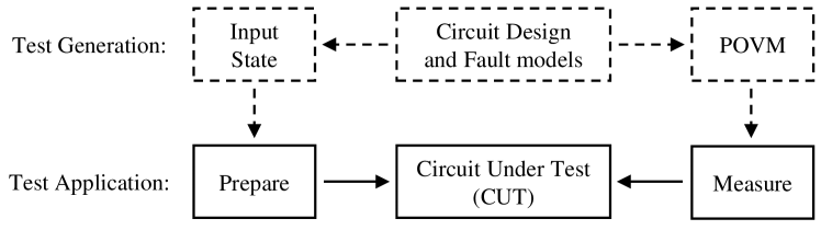
Figure 1: Components of quantum circuit testing.

For classical circuits, an ATPG algorithm faces two challenging tasks: fault-excitation and fault-propagation. The former aims to find the input patterns that can generate suitable value at the wire before the fault site, and the latter lets the output difference of the fault site be reflected at the circuit output. At the first glance, one may believe that the reversibility of quantum circuits makes the fault-excitation and fault-propagation always possible and straightforward. But actually it is hard to directly apply the classical ATPG algorithms on quantum circuits. There are at least three difficulties that hinder the quantum ATPG algorithms.

1. The probabilistic nature and inherent uncertainty of quantum mechanisms make it difficult for us to read-out all information from a given quantum state. Though the quantum state tomography [9, 10] is able to reconstruct the classical description of the given quantum state, the number and complexity of required experiments can be prohibitive. Thus the output analysis for quantum circuits is generally much harder than that for classical circuits.

2. The variety of quantum fault models make the fault analysis rather complicated. For example, the fault effect can be a small rotation on any direction, e.g. small perturbation on the phase, so that the detection of such fault could be very difficult and inefficient.

3. The complexity of implementing the test state and test measurement makes the quantum test equipment (i.e., the quantum equipment for test application, see Fig. 1) itself more likely to be faulty or contain non-negligible noises. This is because the input test pattern can be a highly entangled state, and the corresponding state-preparation circuit can be as complicated as the circuit under test (CUT). To see this, let us consider a simple case: suppose the fault-site is at the end of the circuit, and the state that can excite the fault is simply $|0\rangle$. Then, the state-preparation circuit can trivially be $U^{-1}$ where $U$ is the unitary representing the CUT. Obviously $U^{-1}$ and $U$ have the same circuit complexity (up to a constant scalar). Similarly, the measurement circuit corresponding to the output test pattern could also be as complicated as the CUT. There is no reason to believe that such as-complicated-as-CUT testing circuits are fault-free and will not introduce extra error in the testing process.

The first two difficulties have been partially addressed in several seminal works on quantum ATPG. Paler et al. [11] proposed the Binary Tomographic Test (BTT) which meets the probabilistic nature of quantum circuits. A BTT is a pair of test input state and test measurement. They first simulate both fault-free and faulty quantum circuits on the BTTs, and store the corresponding output distributions. Then the CUT is run many times on the same BTTs. The output distributions are analyzed and compared with the simulation results to detect the faults. However, in [11], both test states and test measurements are simply chosen to be the computational basis, which makes the test inefficient and even unable to detect some important types of fault (e.g. fault in the phase). Bera [12] improved the BTT algorithm to account for the variety of quantum fault models. He adopts the unitary discrimination protocol [13] with Helstrom measurement [14], where the input state and measurement are adaptively chosen for a specific fault, so that an arbitrary single fault can be detected efficiently. However, the complexity of implementing the input state and measurement is not considered in [12], which makes the method difficult to use in practice.

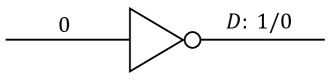
(a) Stuck-at-0 fault

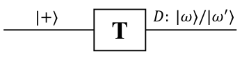
(b) Missing gate fault

Figure 2: An example of the quantum analogue of classical $D$-value.

In this paper, we propose a novel framework of quantum ATPG in which the aforementioned difficulties can be handled in a principled way. To motivate our approach, let us begin by considering an quantum analogue of the classical D-algorithm. Suppose at the fault-site, say quantum gate $U_{i}$, we have a fault model $U^{\prime}_{i}$. By the unitary discrimination protocol [13] and Helstrom measurement [14], we can obtain the optimal input state $|\psi\rangle$ and optimal projective measurement $\{|\omega\rangle\!\langle\omega|,|\omega^{\prime}\rangle\!\langle\omega^{\prime}|\}$ for distinguishing between $U_{i}$ and $U^{\prime}_{i}$. We argue that this measurement is analogue to the $D$-value in the classical D-method. Indeed, this measurement can be seen as a composite “logical value” $|\omega\rangle/|\omega^{\prime}\rangle$ where the first entry $|\omega\rangle$ represents the “value” of fault-free gate and the second entry $|\omega^{\prime}\rangle$ represents the “value” of faulty gate. Note that the “value” here does not indicate the exact quantum state but the optimal measurement for distinguishing the fault-free and faulty states. This is because in an operational view of quantum theory, the fault-effect is no more than the optimal measurement for this specified fault. To be more specific, a simple example is shown in Fig. 2, where $|+\rangle$ is the optimal input state for distinguishing the $T$ gate and the identity gate (i.e., missing gate), $|\omega\rangle/|\omega^{\prime}\rangle$ corresponds to the Helstrom measurement for distinguishing quantum states $T|+\rangle$ and $|+\rangle$.

Similar to the D-algorithm, our next step is to propagate both $|\psi\rangle$ and $|\omega\rangle/|\omega^{\prime}\rangle$ to the primary input and output of the circuit. But as pointed out above, the major issue in the quantum case is not how to propagate the fault effect to the circuit input and output as the quantum circuits are always reversible and thus the propagation can be straightforward. Instead, what concerns us is the complexity of the input and output test patterns (see the above discussions on difficulty (3)). To tackle this issue, we propose to employ the Clifford-only circuits for test application. The reason is three-fold:

1. The Clifford gates are believed to be nearly ideal [15] in the fault-tolerant quantum computation based on stabilizer codes, as the Clifford gates have rather robust and cheap implementation [16, 17].

2. Any Clifford operation can be efficiently synthesized to a relatively small Clifford circuit with size no more than $O(n^{2}/\log n)$ [18, 19], where $n$ is the number of qubits.

3. The Clifford-universal gate set (e.g. Hadamard, Phase and controlled-NOT) is finite and discrete. Thus the Clifford gates can be carefully calibrated on specific quantum devices. This contrasts with the continuous rotation gates such as those in the QFT circuit.

The above advantages ensure that using the Clifford circuits for testing is much simpler and more robust than using general quantum circuits. Based on this observation, we introduce the stabilizer projector decomposition (SPD) to represent the test pattern. By applying a sampling algorithm on the SPD, the test application can be constructed using Clifford-only circuits with classical randomness. It is worth noting that here we use classical randomness rather than quantum randomness (i.e., superposition) because preparing an arbitrary superposition state is much harder than sampling from the corresponding classical distribution. The number of required experiments in our sampling algorithm is explicitly related to the 1-norm metric of SPD. The optimal SPD (i.e., that with minimal 1-norm) for given test pattern can be obtained by solving a convex optimization problem. But in general, it is practically intractable to solve this optimization problem due to the exponentially growing of the problem size, or more specifically, the number of stabilizer projectors. To mitigate this issue, we propose an SPD generation algorithm with several acceleration techniques, where both locality and sparsity are exploited in the SPD calculation. It is proved that the locality exploiting algorithm is optimal in the sense that it reveals the most locality of given SPD, under some mild conditions.

To demonstrate the effectiveness and efficiency of our approach, the overall quantum ATPG framework and the proposed SPD generation algorithm are implemented and evaluated on several commonly used benchmark circuits in IBM Qiskit. The code is available at Github.

The paper is organized as follows. In Section II, the main technical tools needed in this paper are reviewed, including quantum circuits and the fault models, unitary discrimination protocol and the corresponding test pattern, stabilizer formalism and Clifford gates. In Section III, the notion of stabilizer projector decomposition (SPD) with a sampling algorithm is proposed to implement the robust quantum test application. In Section IV, an SPD generation algorithm is developed, with several practical acceleration techniques and certain theoretical guarantees. In Section V, the proposed algorithms are implemented and evaluated on several commonly used benchmark circuits in IBM Qiskit. In Section VI, we summarize the contributions of this work and provide an outlook for future work. Due to the limited space, the proofs of all lemmas, propositions and theorems are omitted in the main text but given in the Appendix.

II Preliminaries

II-A Quantum Circuits and Fault Models

Let us first recall the notion of quantum circuit and its fault models. Classical digital circuits from logic gates acting on boolean variables. Similarly, quantum circuits are made up of quantum (logic) gates on qubits (quantum bits). Using the Dirac notation, a (pure) state of a single qubit is represented by $|\psi\rangle=\alpha_{0}|0\rangle+\alpha_{1}|1\rangle$ with complex numbers $\alpha_{0}$ and $\alpha_{1}$ satisfying $|\alpha_{0}|^{2}+|\alpha_{1}|^{2}=1$. More generally, a state of $n$ qubits can be written as a superposition of $n$-bit strings:

$$|\psi\rangle=\sum_{x\in\{0,1\}^{n}}\alpha_{x}|x\rangle$$ (1)

where complex numbers $\alpha_{x}$ satisfies the normalization condition $\sum_{x}|\alpha_{x}|^{2}=1$. If we identify a string $x=x_{1}...x_{n}\in\{0,1\}^{n}$ with the integer $x=\sum_{i=1}^{n}x_{i}\cdot 2^{i-1}$, then state (1) can also be represented by the $2^{n}$-dimensional column vector $|\psi\rangle=(\alpha_{0},\ldots,\alpha_{2^{n}-1})^{T}$.

A quantum gate on $n$ qubits is mathematically described by a $2^{n}\times 2^{n}$ unitary matrix $U=\{u_{ij}\}$ satisfying $U^{\dagger}U=I_{n}$, where $U^{\dagger}$ stand for the conjugate transpose of $U$ and $I_{n}$ the identity matrix of dimension $2^{n}$ (we may omit the subscript of $I_{n}$ when it does not cause confusion). If state $|\psi\rangle$ is input to this gate, then the output from the gate is the state represented by column vector $|\psi^{\prime}\rangle=U|\psi\rangle$. Thus, a quantum circuit is a sequence of quantum gates: $(U_{1},\ldots,U_{d})$, where $d\geq 1$, and $U_{i}\,\,(1\leq i\leq d)$ are quantum gates. We will use $U_{i:j}\,\,(i\leq j)$ to denote the unitary matrix corresponding to the circuit slice from $i$-th gate to $j$-th gate; that is, $U_{i:j}=U_{j}\ldots U_{i+1}U_{i}$.

Hadamard:    @C=1.0em @R=0.65em @!R & H $\frac{1}{\sqrt{2}}\begin{bmatrix}1&1\\ 1&-1\end{bmatrix}$

(a)

Pauli-X (NOT):    @C=1.0em @R=0.65em @!R & X $\,\quad\begin{bmatrix}0&1\\ 1&0\end{bmatrix}$

(b)

Controlled-NOT:   @C=1.0em @R=0.65em @!R & 1
$\begin{bmatrix}1&0&0&0\\ 0&1&0&0\\ 0&0&0&1\\ 0&0&1&0\end{bmatrix}$

(c)

Figure 3: Examples of single and multi-qubit quantum gates.

Example 1 (Quantum Gates).

Some commonly used quantum gates are shown in Fig. 3, including:

1. Single-qubit quantum gates such as the Hadamard gate and Pauli-X (NOT) gate.

2. Multi-qubit quantum gates such as the controlled-NOT (CNOT) gate.

In this work, we adopt the single-fault assumption typically used in test generation and evaluation for both classical circuits [20] and quantum circuits [11, 12]: there can be only one fault in the circuit. Let $U_{\text{\tiny{CUT}}}:=(\tilde{U}_{1},\ldots,\tilde{U}_{d})$ be the circuit under test (CUT). Each gate $\tilde{U}_{i}$ is specified by its fault-free version $U_{i}$ and is potentially to be faulty. We assume that its fault model $U^{\prime}_{i}$ is known in advance. Our goal is to determine whether the given CUT is fault-free or faulty. In this work, we adopt the single-fault assumption (i.e., the cause of a circuit failure is attributed to only one faulty gate), which is typically used for both classical [20] and quantum[11, 12] circuits.

II-B Discrimination of Quantum Gates

A basic step in quantum ATPG is to discriminate a gate $U_{i}$ from its faulty version $U_{i}^{\prime}$. This problem has been well studied by the quantum information community [13, 14, 21]. A general manner is by inputting a mixed state $\rho$ to this unknown unitary and then performing the measurement to obtain the result. Mathematically, the distinguishability between $U_{i}\rho U_{i}^{\dagger},U^{\prime}_{i}\rho{U^{\prime}}_{i}^{{\dagger}}$, i.e., the trace distance $tr(|U_{i}\rho U_{i}^{\dagger}-U^{\prime}_{i}\rho{U^{\prime}}_{i}^{{\dagger}}|)$ by the Holevo-Helstrom theorem [14, 21], must be maximized. Due to the convexity of trace distance, the optimal input can always be achieved by a pure state $\rho=|\psi\rangle\!\langle\psi|$. Thus the problem is equivalent to minimizing the inner product of $U_{i}|\psi\rangle$ and $U^{\prime}_{i}|\psi\rangle$:

$$\min_{|\psi\rangle}\big{|}\langle\psi|U_{i}^{\dagger}U^{\prime}_{i}|\psi\rangle\big{|}$$ (2)

Let the spectral decomposition of $U_{i}^{\dagger}U^{\prime}_{i}$ be $\sum_{i}\lambda_{i}|v_{i}\rangle\!\langle v_{i}|$, and $|\psi\rangle=\sum_{i}\alpha_{i}|v_{i}\rangle$. Then it becomes:

$$\min_{|\psi\rangle}\bigg{|}\sum_{i}\lambda_{i}\langle{\psi}|{v_{i}}\rangle\langle{v_{i}}|{\psi}\rangle\bigg{|}=\min_{\sum|\alpha_{i}|^{2}=1}\bigg{|}\sum_{i}\lambda_{i}|\alpha_{i}|^{2}\bigg{|}$$ (3)

This optimization problem can be solved by quadratic programming.

After obtaining the optimal input state $|\overline{\psi}\rangle$, the optimal measurement for distinguishing between the pair $|\psi\rangle=U_{i}|\overline{\psi}\rangle,\ |\psi^{\prime}\rangle=U_{i}^{\prime}|\overline{\psi}\rangle$ of output states of the two gates can be achieved by their Helstrom measurement. More specifically, assume $\langle{\psi}|{\psi^{\prime}}\rangle=re^{i\theta}$ and define:

$$\begin{split}&|\omega\rangle=\frac{1}{\sqrt{2}}\bigg{(}\frac{|\psi\rangle+e^{-i\theta}|\psi^{\prime}\rangle}{\||\psi\rangle+e^{-i\theta}|\psi^{\prime}\rangle\|}+\frac{|\psi\rangle-e^{-i\theta}|\psi^{\prime}\rangle}{\||\psi\rangle-e^{-i\theta}|\psi^{\prime}\rangle\|}\bigg{)}\\ &|\omega^{\prime}\rangle=\frac{1}{\sqrt{2}}\bigg{(}\frac{|\psi\rangle+e^{-i\theta}|\psi^{\prime}\rangle}{\||\psi\rangle+e^{-i\theta}|\psi^{\prime}\rangle\|}-\frac{|\psi\rangle-e^{-i\theta}|\psi^{\prime}\rangle}{\||\psi\rangle-e^{-i\theta}|\psi^{\prime}\rangle\|}\bigg{)}\end{split}$$ (4)

Then the Helstrom measurement is the measurement in basis states $|\omega\rangle$ and $|\omega^{\prime}\rangle$, or more precisely the measurement with two measurement operators $\{|\omega\rangle\!\langle\omega|,|\omega^{\prime}\rangle\!\langle\omega^{\prime}|\}$. Actually, if we define the order $A\sqsubseteq B$ between two matrices $A$ and $B$ by requiring that $B-A$ is positive semi-definite, then any POVM measurement with measurement operators $\{M,I-M\}$ satisfying $M\sqsupseteq|\omega\rangle\!\langle\omega|,I-M\sqsupseteq|\omega^{\prime}\rangle\!\langle\omega^{\prime}|$ is optimal for discriminating states $|\psi\rangle$ and $|\psi^{\prime}\rangle$.

II-C Test Patterns for Single-Fault Quantum Circuits

The above discussion considers gate-level discrimination, which only involves a small sub-system. Now we move on to consider how to distinguish the fault-free circuit and a faulty circuit. It is impractical to solve the optimization problem (3) for the whole circuit due to the exponential growth of dimension. Instead, we should locally solve the discrimination problem for $U_{i}$ and $U^{\prime}_{i}$, where the dimension is $2^{m}$ in which $m$ is the number of qubits involved in gates $U_{i}$ and $U^{\prime}_{i}$ and is generally small (say, a single qubit or two qubits). Then we can simply propagate the fault excitation signal and fault effect (i.e., state $|\psi\rangle\!\langle\psi|$ and measurement $\{|\omega\rangle\!\langle\omega|,|\omega^{\prime}\rangle\!\langle\omega^{\prime}|\}$ obtained in Subsection II-B) to the beginning and end of the circuit respectively. Formally, we have:

Proposition 1.

If quantum state $\rho$ and projective measurement $M$ satisfies the following conditions:

$$\begin{gathered}\rho\sqsubseteq U_{1:i-1}^{\dagger}\,(Q\otimes|\psi\rangle\!\langle\psi|)\,U_{1:i-1}\\ U_{i+1:d}\,(Q\otimes|\omega\rangle\!\langle\omega|)\,U^{\dagger}_{i+1:d}\sqsubseteq M\\ U_{i+1:d}\,(Q\otimes|\omega^{\prime}\rangle\!\langle\omega^{\prime}|)\,U^{\dagger}_{i+1:d}\sqsubseteq I-M\end{gathered}$$ (5)

for some projection $Q$ on the state space of the qubits that are not in gates $U_{i}$ and $U^{\prime}_{i}$, then they are optimal as the input state and the measurement at the end of circuit for detecting the fault.

We call a pair $(\rho,M)$ of input state $\rho$ and measurement $M$ satisfying conditions (5) a test pattern of CUT $C$ with respect to faulty version $C_{i}$. For simplicity, we can choose test pattern $(\rho,M)$ defined by

$$\begin{gathered}\rho=U^{{\dagger}}_{1:i-1}\big{(}\frac{Q}{\textup{tr}(Q)}\otimes|\psi\rangle\!\langle\psi|\big{)}U_{1:i-1}\\ M=U_{i+1:d}\big{(}Q\otimes|\omega\rangle\!\langle\omega|\big{)}U^{\dagger}_{i+1:d}.\end{gathered}$$ (6)

In particular, $Q=I$ (the idenity operator on the state space of the qubits that are not in $U_{i}$ and $U^{\prime}_{i}$) is a practical choice for computational efficiency. This is because $I$ is invariant under any gate $U_{j}$; that is $U_{j}IU_{j}^{\dagger}=I$.

II-D Stabilizer Formalism and Clifford Gates

As discussed in Section I and explicitly shown in Proposition 1, in quantum ATPG, the backward propogation and forward propagation of fault effect are straightforward, and the major challenge is to find efficient implementation of a test pattern, including the preparation of the input state $\rho$ and implementation of the output measurement $M$. Our solution to this problem is based on the stabilizer formalism and Clifford gates widely used in quantum error correction and fault-tolerant quantum computation. For convenience of the reader, we review basics of them in this subsection.

II-D1 Pauli Operators

Pauli operators are widely used in quantum computation and quantum information [22]. Single-qubit Pauli operators consist of $I,X,Y,Z$ where

$$X=\begin{bmatrix}0&1\\ 1&0\end{bmatrix},\,Y=\begin{bmatrix}0&-i\\ i&0\end{bmatrix},\,Z=\begin{bmatrix}1&0\\ 0&-1\end{bmatrix}$$ (7)

Any $n$-qubit Pauli operator $P$ is of the form:

$$P_{1}\otimes P_{2}\otimes\cdots\otimes P_{n}$$ (8)

where each $P_{i}$ is chosen from $I,X,Y,Z$. We will use $X_{i}$ (or $Y_{i},Z_{i}$) to denote the Pauli operator $P_{1}\otimes\cdots\otimes P_{n}$ with $P_{i}=X$ (or $Y,Z$) and $P_{j}=I$ for all $j\neq i$. Suppose $P$ is a Pauli operator, we will use $\underline{e^{i\theta}P}$ to denote the Pauli operator by simply discarding the phase $e^{i\theta}$, (e.g. $\underline{ZX}=\underline{iY}=Y$). We call $e^{i\theta}P$ a signed Pauli operator, if $\theta\in\{0,\pi\}$ and $P$ is a Pauli operator. Without causing confusion, the same letters (e.g. $P,Q$) may be used to denote either Pauli or signed Pauli operators. Note that any two (signed) Pauli operators $P,Q$ are either commute (i.e., $PQ=QP$) or anti-commute (i.e., $PQ=-QP$).

There is a very useful representation for the Pauli operators, using the vectors over $\textup{GF}(2)$. In this paper, we use $00,01,10,11$ to represent $I,Z,X,Y$ respectively. The Pauli operator $P=P_{1}\otimes\ldots\otimes P_{n}$ is then represented by the vector $v(P)=(v_{1},\ldots,v_{2n})$, where $v_{2i-1},v_{2i}$ corresponds to the representation of $P_{i}$. Note that the vector addition coincides with the Pauli operator multiplication up to a global phase. That is, if $\underline{PQ}=R$ where $P,Q,R$ are Pauli operators, then $v(P)+v(Q)=v(R)$. For a signed Pauli operator $P$, we simply define its vector representation as $v(\underline{P})$. We say that a set of (signed) Pauli operators are independent if their vector representations are independent.

II-D2 Stabilizer Formalism

We say that a state $|\psi\rangle$ is stabilized by a signed Pauli operator $P$ if $P|\psi\rangle=|\psi\rangle$. In this case, $P$ is called the stabilizer of $|\psi\rangle$. The basic idea of the stabilizer formalism is that many quantum states can be more easily described by their stabilizers [22].

Example 2 (Pauli Stabilizer).

Consider the EPR state

$$|\psi\rangle=\frac{|00\rangle+|11\rangle}{\sqrt{2}}$$ (9)

We can verify that $|\psi\rangle$ is the unique quantum state (up to global phase) stabilized by Pauli operators $X_{1}X_{2}$ and $Z_{1}Z_{2}$. Thus $|\psi\rangle$ can be described by its stabilizers $\{X_{1}X_{2},Z_{1}Z_{2}\}$.

In general, suppose $G$ is a group of $n$-qubit signed Pauli operators and $-I\notin G$. We call $G$ the stabilizer group. Let $V$ be the set of all $n$-qubit states which are stabilized by every element of $G$. Then $V$ forms a vector space. The projector $S$ onto $V$ is called the stabilizer projector corresponding to group $G$. When $V$ is one-dimensional, its projector $S$ is of the form $S=|\phi\rangle\!\langle\phi|$ and $|\phi\rangle$ is called the stabilizer state corresponding to $G$. A set of elements $P_{1},\ldots,P_{l}$ is said to be the generators of $G$ if every element of $G$ can be written as a product of elements from the list $P_{1},\ldots,P_{l}$, and we write $G=\langle P_{1},\ldots,P_{l}\rangle$. There are some useful properties of the stabilizer formalism. First, the elements of $G$ commute, i.e., for any $P,Q\in G$, $PQ=QP$. Second, the stabilizer projector $S$ can be represented by

$$S=\prod_{i=1}^{l}\frac{I+P_{i}}{2}=\frac{1}{|G|}\sum_{P_{i}\in G}P_{i}$$ (10)

where $P_{1},\ldots,P_{l}$ are the generators of $G$.

II-D3 Clifford Operation

Suppose we apply a unitary $U$ to the stabilizer space $V$. Let $|\phi\rangle\in V$. Then for any $g\in G$:

$$U|\phi\rangle=Ug|\phi\rangle=UgU^{\dagger}U|\phi\rangle$$ (11)

which means that $U|\phi\rangle$ is stabilized by $UgU^{\dagger}$. Thus subspace $UV$ is stabilized by the group $UGU^{\dagger}\equiv\{UgU^{\dagger}|g\in G\}$ and the corresponding stabilizer projector is $USU^{\dagger}$. For a unitary $U$, if it takes signed Pauli operators to signed Pauli operators under conjugation, i.e., $UPU^{\dagger}=P^{\prime}$, then we call it a Clifford operation. This transformation takes on a particularly appealing form. That is, for any stabilizer projector $S$, $USU^{\dagger}=S^{\prime}$ where $S^{\prime}$ is also a stabilizer projector. It was proved that any $n$-qubit Clifford operation can be implemented using Hadamard, Phase and CNOT gates, with the circuit size no more than $O(n^{2}/\log n)$ [18].

Example 3 (Clifford Gate).

Hadamard gate is Clifford:

$$HXH^{\dagger}=Z,\,\,HYH^{\dagger}=-Y,\,\,HZH^{\dagger}=X$$ (12)

Clifford circuits can be efficiently simulated on a classical computer according to the Gottesman-Knill theorem [23]. Furthermore, using fault-tolerant techniques based on CSS codes, including the popular Steane code and surface codes, they can be efficiently implemented with little error rate [16, 17]. This contrasts with the non-Clifford gates (e.g. $T$ gate), which incur more than a hundred times cost for fault-tolerant implementation.

The following facts about Clifford operations will be needed in this paper:

Lemma 1.

Given two sets of signed Pauli operators $\{P_{1},\ldots,P_{n}\}$ and $\{Q_{1},\ldots,Q_{n}\}$. If

1. $\forall i,j\leq n$, $P_{i},P_{j}$ commute $\Longleftrightarrow$ $Q_{i},Q_{j}$ commute,

2. $\{P_{1},\ldots,P_{n}\}$, $\{Q_{1},\ldots,Q_{n}\}$ are both independent

then there is a Clifford unitary $U$ with $UP_{i}U^{\dagger}=Q_{i}$ for all $i$.

Corollary 1.

For any stabilizer projector $A$ of rank $2^{m}$ in an $n$-qubit system, there is a Clifford circuit $U_{A}$ such that $U_{A}(|0\rangle\!\langle 0|^{\otimes n-m}\otimes I)U_{A}^{\dagger}=A$.

III Robust Quantum Test Application

For classical circuits, test application is the process of applying a test pattern obtained from test generation to the CUT and analyzing the output responses [20]. In the quantum case, given a test pattern $(\rho,M)$, the test application aims to estimate the expected outcomes of the test pattern on the CUT, i.e., $\textup{tr}(MU_{\text{\tiny{CUT}}}\rho U_{\text{\tiny{CUT}}}^{\dagger})$.

III-A Stabilizer Projector Decomposition

As mentioned in Subsection II-D, Clifford operations have reliable and efficient fault-tolerant implementation. Then we choose to use Clifford-only circuit to realize our test application. However, a test pattern $(\rho,M)$ as a solution of Equation (5) is generally non-Clifford. To handle this problem, we introduce the stabilizer projector decomposition (SPD), which generalizes the notion of pseudo-mixtures for stabilizer states [24].

Definition 1 (Stabilizer Projector Decomposition, SPD).

Let $0\sqsubseteq A\sqsubseteq I$. Then a stabilizer projector decomposition (SPD for short) of $A$ is a finite set $\mathcal{A}=\{(a_{i},A_{i})\}_{i}$ such that

$$A=\sum_{i}a_{i}A_{i},$$

where $A_{i}$ are stabilizer projectors and $a_{i}$ are real numbers.

We will use the calligraphic letters (e.g. $\mathcal{A},\mathcal{B}$) to denote the SPDs and use $\textup{SPD}(A)$ to denote the set of all possible SPDs of operator $A$. For convenience, given an SPD $\mathcal{A}=\{(a_{i},A_{i})\}$, we use $Q\otimes\mathcal{A}$ to denote the SPD $\{(a_{i},Q\otimes A_{i})\}$, where $Q$ is a stabilizer projector. Similarly, we write $U\mathcal{A}U^{\dagger}$ for the SPD $\{(a_{i},UA_{i}U^{\dagger})\}$ and $c\mathcal{A}$ for the SPD $\{(c\cdot a_{i},A_{i})\}$ where $U$ is a Clifford unitary, and $c$ is a real number. We also define:

$$\textup{tr}(\mathcal{A})=\textup{tr}(\sum_{i}a_{i}A_{i}).$$

In our SPD-based sampling algorithm, the following norms are needed.

Definition 2 (Norms of SPD).

The 1-norm $\nu$ and weighted 1-norm $\nu^{*}$ of SPD $\mathcal{A}=\{(a_{i},A_{i})\}$ are defined by:

$$\small\begin{gathered}\nu(\mathcal{A})=\sum_{i}|a_{i}|\\ \nu^{*}(\mathcal{A})=\sum_{i}|a_{i}|\textup{tr}A_{i}\end{gathered}$$ (13)

III-B SPD-based Sampling Algorithm for Test Application

Now we turn to the main problem in this section: estimate the expectation $\textup{tr}(MU_{\text{\tiny{CUT}}}\rho U_{\text{\tiny{CUT}}}^{\dagger})$ for a given test pattern $(\rho,M)$. Here we assume that the SPDs $\mathcal{A},\mathcal{B}$ for $\rho,M$ are provided, respectively:

$$\begin{gathered}\rho=\sum_{i}a_{i}A_{i}\\ M=\sum_{i}b_{i}B_{i}\end{gathered}$$ (14)

but leave the problem of generating them to the next section.

First, we can rewrite the expectation under estimation in terms of the given SPDs:

$$\begin{split}\textup{tr}(MU_{\text{\tiny{CUT}}}\rho U_{\text{\tiny{CUT}}}^{\dagger})&=\sum_{ij}a_{i}b_{j}\textup{tr}(B_{j}U_{\text{\tiny{CUT}}}A_{i}U_{\text{\tiny{CUT}}}^{\dagger})\\ &=\sum_{ij}a_{i}b_{j}\textup{tr}A_{i}\textup{tr}(B_{j}U_{\text{\tiny{CUT}}}\frac{A_{i}}{\textup{tr}A_{i}}U_{\text{\tiny{CUT}}}^{\dagger})\end{split}$$ (15)

For simplicity, we put:

$$\textup{tr}_{ij}=\textup{tr}(B_{j}U_{\text{\tiny{CUT}}}A_{i}/\textup{tr}A_{i}U_{\text{\tiny{CUT}}}^{\dagger}).$$

Since $A_{i},B_{j}$ are stabilizer projectors, by Corollary 1, we can implement the state preparation of $A_{i}/\textup{tr}A_{i}$ and projective measurement of $B_{j}$ using Clifford-only circuits. Then, we can sample from the Bernoulli distribution of parameter $\textup{tr}_{ij}$, by applying the CUT on input state $A_{i}/\textup{tr}A_{i}$ and sampling the result according to measurement $B_{j}$.

To further estimate $\sum_{ij}a_{i}b_{j}\textup{tr}A_{i}\textup{tr}_{ij}$, we use the quasi-probability distribution [24, 25] $\{a_{i}b_{j}\textup{tr}A_{i}\}_{ij}$ to form a true probability distribution $\{p_{ij}\}_{ij}$, where

$$p_{ij}=|a_{i}b_{j}\textup{tr}A_{i}|/\sum_{k}|a_{k}\textup{tr}A_{k}|\sum_{k}|b_{k}|.$$

In each single trial, we sample $i,j$ from this probability distribution $p_{ij}$ and then sample a result $m\in\{0,1\}$ from the Bernoulli distribution of parameter $\textup{tr}_{ij}$. We do not record $m$ but its corrected version:

$$\begin{split}\hat{m}&=m\cdot\textup{sign}(a_{i}b_{j})(\sum_{k}|a_{k}|\textup{tr}A_{k})(\sum_{k}|b_{k}|)\\ &=m\cdot\textup{sign}(a_{i}b_{j})\nu^{*}(\mathcal{A})\nu(\mathcal{B})\end{split}$$ (16)

where $\textup{sign}(x)=1$ if $x\geq 0$ and $\textup{sign}(x)=-1$ otherwise. Note that $\hat{m}$ is essentially sign-corrected by $\textup{sign}(a_{i}b_{j})$ and modulus-corrected by $\nu^{*}(\mathcal{A})\nu(\mathcal{B})$. The expected value of random variable $\hat{m}$ is

$$\begin{split}E(\hat{m})&=\sum_{ij}p_{ij}\textup{tr}_{ij}\textup{sign}(a_{i}b_{j})(\sum_{k}|a_{k}|\textup{tr}A_{k})(\sum_{k}|b_{k}|)\\ &=\sum_{ij}a_{i}b_{j}\textup{tr}A_{i}\textup{tr}_{ij}=\textup{tr}(MU_{\text{\tiny{CUT}}}\rho U_{\text{\tiny{CUT}}}^{\dagger})\end{split}$$ (17)

This means $\hat{m}$ can serve as an unbiased estimator of the target value $\textup{tr}(MU_{\text{\tiny{CUT}}}\rho U_{\text{\tiny{CUT}}}^{\dagger})$. By repeating this sampling process, we can estimate the result to any desired accuracy, where the number of repetition depends on the variance of $\hat{m}$. The details of this SPD-based sampling algorithm are summarized in Algorithm 1.

Note that $\hat{m}\in[-\nu^{*}(\mathcal{A})\nu(\mathcal{B}),\nu^{*}(\mathcal{A})\nu(\mathcal{B})]$. By the Hoeffding’s inequality, we know that

$$\frac{2}{\delta^{2}}\ln(\frac{2}{\epsilon})\big{[}\nu^{*}(\mathcal{A})\nu(\mathcal{B})\big{]}^{2}$$ (18)

samples are needed to estimate the result with error less than $\delta$ and success probability exceeding $1-\epsilon$.

Algorithm 1 SPD-based sampling algorithm

1:SPD for $\rho,M$ (see Equation (14)), Quantum CUT $U_{\text{\tiny{CUT}}}$, required precision $\delta$ and success probability $1-\epsilon$

2:An estimation $m$ of $\textup{tr}(MU_{\text{\tiny{CUT}}}\rho U_{\text{\tiny{CUT}}}^{\dagger})$

3:Initialize the estimation result $m\leftarrow 0$.

4:Set the iteration number $T\leftarrow\frac{2}{\delta^{2}}\ln(\frac{2}{\epsilon})[\nu^{*}(\mathcal{A})\nu(\mathcal{B})]^{2}$

5:for $t=1,2,\ldots,T$ do

6:    Sample values $i$ and $j$ from distribution $|a_{i}|\textup{tr}A_{i}/\nu^{*}(\mathcal{A})$ and $|b_{j}|/\nu(\mathcal{B})$ respectively.

7:    Uniformly sample value $l\in\{0,\ldots,\textup{tr}A_{i}-1\}$

8:    Initialize the first $n-\log\textup{tr}A_{i}$ qubits to $|0\rangle$, and last $\log\textup{tr}A_{i}$ qubits to $|l\rangle$.

9:    Apply the Clifford circuit $U_{A_{i}}$. $\triangleright$ Corollary 1

10:    Apply the CUT $U_{\text{\tiny{CUT}}}$.

11:    Apply the Clifford circuit $U^{\dagger}_{B_{j}}$. $\triangleright$ Corollary 1

12:    Measure the first $n-\log\textup{tr}B_{j}$ quibts on computational basis.

13:    if The measurement result is $|0\rangle$ then

14:         $m\leftarrow m+\textup{sign}(a_{i}b_{j})\nu^{*}(\mathcal{A})\nu(\mathcal{B})$

15:    end if

16:end for

17:$m\leftarrow m/T$

18:return $m$

Theorem 1.

Algorithm 1 estimates $\textup{tr}(MU_{\text{\tiny{CUT}}}\rho U_{\text{\tiny{CUT}}}^{\dagger})$ to additive error $\delta$ with probability larger than $1-\epsilon$, and runs in

$$O\bigg{(}\frac{\ln(1/\epsilon)}{\delta^{2}}\big{[}\nu^{*}(\mathcal{A})\nu(\mathcal{B})\big{]}^{2}\bigg{)}$$ (19)

IV SPD generation

In the previous section, an algorithm for robust test application was presented under the assumption that the SPDs of input state $\rho$ and measurement $M$ in the test pattern are given. This section is devoted to solving the remaining problem, namely SPD generation.

As shown in Theorem 1, we need to generate the SPDs that have as less $\nu$ (or $\nu^{*}$) value as possible. In this sense, given a positive operator $A$, one can find the $\nu$-optimal SPD by solving this convex optimization problem:

$$\begin{gathered}\min_{x}\quad\|x\|_{1}\\ \textup{subject to}\quad Mx=b\end{gathered}$$ (20)

where $M_{ij}=\textup{tr}(P_{i}S_{j})$, $b_{i}=\textup{tr}(P_{i}A)$, $P_{i}$ is the $i$-th Pauli operator and $S_{j}$ is the $j$-th stabilizer projector. An optimal solution $x$ of problem (20) indicates a $\nu$-optimal SPD $\{(x_{i},S_{i})\}$ for $A$. For computational efficiency, we can discard those $(x_{i},S_{i})$ with $x_{i}=0$. Similarly, we can obtain the $\nu^{*}$-optimal SPD by solving this convex optimization problem:

$$\begin{gathered}\min_{x}\quad\|w\circ x\|_{1}\\ \textup{subject to}\quad Mx=b\end{gathered}$$ (21)

where $w_{i}=\textup{tr}(S_{i})$ and $\circ$ denotes the element-wise product.

IV-A Locality Exploiting

However, the optimization problems (20), (21) are practically intractable since the number of stabilizer projectors grows exponentially [26]. To circumvent this difficulty, we exploit the locality in the SPD generation. Roughly speaking, we first solve the optimization problem locally for the subsystem at the fault-site, obtaining an SPD with a local form. Then, we forward (backward) propagate the fault effect (excitation signal) represented by SPD to the end (beginning) of the circuit, as with the D-algorithm, while keep exploiting the SPD’s locality. The idea is, 1) using a Clifford unitary $U_{C}$ to map the current SPD to a local form, 2) solving problem (20) or (21) in the “non-trivial” subsystem, and 3) mapping back. The optimality is preserved thanks to the nice properties of $\nu$ (and also $\nu^{*}$ analogously), i.e., the Clifford invariance (C-Inv) and tensor invariance (T-Inv):

1. C-Inv: For any Clifford unitary $U_{C}$, if an SPD $\mathcal{A}$ is $\nu$-optimal ($\nu^{*}$-optimal), then $U_{C}\mathcal{A}U_{C}^{\dagger}$ is also $\nu$-optimal ($\nu^{*}$-optimal).

2. T-Inv: For any stabilizer projector $S$, if an SPD $\mathcal{A}$ is $\nu$-optimal ($\nu^{*}$-optimal), then $S\otimes\mathcal{A}$ is also $\nu$-optimal ($\nu^{*}$-optimal).

Specifically, suppose we need to find the $\nu$-optimal (or $\nu^{*}$-optimal) SPD for $UAU^{\dagger}$, and $A$ is represented by an SPD $\mathcal{A}$, then our strategy follows this diagram:

(22)

where $U_{C}$ is a Clifford unitary such that $U\xrightarrow{U_{C}}U_{\bot}\otimes U^{\prime}$ and $\mathcal{A}\xrightarrow{U_{C}}A_{\bot}\otimes\mathcal{A}^{\prime}$ by conjugation, where $U_{\bot}$, $A_{\bot}$ are Clifford unitary and stabilizer projector, which are the “trivial” parts in our computation, and $\bot=U_{\bot}A_{\bot}U_{\bot}^{\dagger}$. The above procedures are summarized in Algorithm 2.

The remaining problem is how to find a good $U_{C}$ that satisfies diagram (22). We propose an algorithm (shown in Algorithm 3) for finding such $U_{C}$ that reveals as many locality as possible. Similar to [27], we assume that the elementary gate set under consideration is contained in the set of Clifford + Pauli rotations (i.e., $e^{i\theta P}$ where $P$ is a Pauli operator and $\theta\in[-\pi,\pi]$). Note that this form covers some important and practical universal quantum gate sets, such as Clifford + T gate set, or more generally the Clifford + Z rotation gate set.

Now, we provide the main intuition behind Algorithm 3 (for simplicity, here we provide the intuition only considering $\mathcal{A}$, without $U$). First note that any stabilizer projector is equivalent to $|0\rangle\!\langle 0|\otimes I$ under Clifford conjugation. Thus, to extract a stabilizer projector $A_{\bot}$ from the SPD $\mathcal{A}$, Algorithm 3 works roughly as follows,

1. extract a rank-1 projector $|0\rangle\!\langle 0|$ (steps 3-8), by computing the intersection of all components in $\mathcal{A}$,

2. extract a full rank projector $I$ (steps 9-20), by computing the complement of the union of all components in $\mathcal{A}$,

3. combine previous results (step 21).

Finally, the algorithm can exploit a smaller “non-trivial” subsystem of size $(s+t)/2$ (see Algorithm 3 for details). Its performance is theoretically guaranteed by the following theorem:

Theorem 2.

Algorithm 3 finds a Clifford unitary $U_{C}$ that satisfies diagram (22). Moreover, if either of the following two conditions is satisfied,

1. $\mathcal{A}$ is $\nu$-optimal and has the smallest $\nu^{*}$ among all other $\nu$-optimal SPDs for $A$

2. $\mathcal{A}$ is $\nu^{*}$-optimal and has the smallest $\nu$ among all other $\nu^{*}$-optimal SPDs for $A$

then $U_{C}$ is optimal (i.e., reveals the minimum “non-trivial” subsystem) among all Clifford unitaries that satisfy diagram (22).

The proof is deferred to the Appendix. Note that both conditions can be easily achieved by multi-objective optimization for Problem (20) and Problem (21), more details are shown in section IV-B1.

Algorithm 2 SPD generation

1:Description of the fault-free circuit $(U_{1},\ldots,U_{d})$, potential fault position $i$ and corresponding fault model $U^{\prime}_{i}$.

2:SPD for $\rho$ and $M$, where $\rho$ and $M$ is the optimal input and measurement that can detect the fault.

3:Let $(|\psi\rangle,|\omega\rangle)$ be the test pattern for distinguishing $U_{i}$ and $U^{\prime}_{i}$. $\triangleright$ see Section II-B

4:Let $\mathcal{A}$ be the $\nu^{*}$-optimal SPD for $|\psi\rangle\!\langle\psi|$ $\triangleright$ Problem (21)

5:Let $\mathcal{B}$ be the $\nu$-optimal SPD for $|\omega\rangle\!\langle\omega|$ $\triangleright$ Problem (20)

6:$\mathcal{A}\leftarrow I\otimes\mathcal{A}$, $\mathcal{B}\leftarrow I\otimes\mathcal{B}$ $\triangleright$ Padding

7:for $j=i-1$ down to $1$ do $\triangleright$ Backward propagation

8:    if $U_{j}$ is Clifford then

9:         $\mathcal{A}\leftarrow U^{\dagger}_{j}\mathcal{A}U_{j}$

10:    else

11:         Let $U_{C}=\text{LOC\_EXPL}(U_{j}^{\dagger},\mathcal{A})$ $\triangleright$ Algorithm 3

12:         $\mathcal{A}\leftarrow$ the optimal SPD computed through diagram (22)

13:    end if

14:end for

15:$\mathcal{A}\leftarrow\mathcal{A}/\textup{tr}(\mathcal{A})$

16:for $j=i+1$ to $d$ do $\triangleright$ Forward propagation

17:    if $U_{j}$ is Clifford then

18:         $\mathcal{B}\leftarrow U_{j}\mathcal{B}U_{j}^{\dagger}$

19:    else

20:         Let $U_{C}=\text{LOC\_EXPL}(U_{j},\mathcal{B})$ $\triangleright$ Algorithm 3

21:         $\mathcal{B}\leftarrow$ the optimal SPD computed through diagram (22)

22:    end if

23:end for

24:return $\mathcal{A},\mathcal{B}$

Algorithm 3 Locality exploiting, LOC_EXPL$(U,\mathcal{A})$

1:Non-Clifford $U$, SPD $\mathcal{A}=\{(a_{i},A_{i})\}_{i=1}^{m}$.

2:Clifford $U_{C}$ that satisfies diagram (22).

3:Suppose $U=e^{i\theta P_{U}}$, $P_{U}$ is a Pauli operator and $|\theta|\leq\pi$

4:Let $G_{i}$ be the group associated to stabilizer projector $A_{i}$

5:Let $\hat{P}_{1},\ldots,\hat{P}_{l}$ be the independent generators of $G_{1}\cap\ldots\cap G_{m}$

6:if $P_{U}$ anti-commutes with some $\hat{P}_{i}$ then

7:    Let $P_{U}$ only anti-commutes with $\hat{P}_{l}$ (exchange the subscripts of $\hat{P}_{i}$ or set $\hat{P}_{i}\leftarrow\hat{P}_{i}\hat{P}_{j}$ if necessary)

8:    $l\leftarrow l-1$

9:end if

10:Generate the Clifford unitary $V_{1}$ that maps $\hat{P}_{1},\ldots,\hat{P}_{l},P_{U}$ to $Z_{1},\ldots,Z_{l},Z_{l+1}$ $\triangleright$ Lemma 1

11:For each $V_{1}G_{i}V_{1}^{\dagger}$, find a set of independent generators of the form $Z_{1},\ldots,Z_{l},I_{l}\otimes P_{i,1},\ldots,I_{l}\otimes P_{i,l_{i}}$

12:Find a maximal independent set $Q_{1},\ldots,Q_{s}$ of $Z_{1},P_{1,1},\ldots,P_{1,l_{1}},\ldots,P_{m,1},\ldots,P_{m,l_{m}}$

13:for $i\leq s,i<j\leq s$ do

14:    if $Q_{i},Q_{j}$ anti-commute then

15:         for $k\leq s,k\neq i,j$ do

16:             If $Q_{k},Q_{i}$ anti-commute, then $Q_{k}\leftarrow\underline{Q_{k}Q_{j}}$

17:             If $Q_{k},Q_{j}$ anti-commute, then $Q_{k}\leftarrow\underline{Q_{k}Q_{i}}$

18:         end for

19:    end if

20:end for

21:Exchange the subscripts of $Q_{1},\ldots,Q_{s}$ so that $Q_{1},\ldots,Q_{t}$ commute with all $Q_{i},i\leq s$ and $Q_{t+2i-1}$ only anti-commutes with $Q_{t+2i}$ for $i=1,\ldots,(s-t)/2$

22:Generate a Clifford unitary $V_{2}$ that maps $Q_{1},\ldots,Q_{t}$ to $Z_{1},\ldots,Z_{t}$ and maps $Q_{t+1},\ldots,Q_{s}$ to $Z_{t+1},X_{t+1},\ldots,Z_{(t+s)/2},X_{(t+s)/2}$ $\triangleright$ Lemma 1

23:$V\leftarrow V_{2}V_{1}$

24:$U_{C}:=V$

25:return $U_{C}$

IV-B Implementation Details

The algorithm presented above still faces some practical challenges in its implementation. In this subsection, we propose several important techniques to meet these challenges and thus improve the feasibility of the algorithm.

IV-B1 Multi-Objective Optimization

To meet the requirements of Theorem 2, we need to obtain an SPD that is primarily $\nu$-optimal and secondarily $\nu^{*}$-optimal in the forward propagation (or primarily $\nu^{*}$-optimal and secondarily $\nu$-optimal in the backward propagation). Consider the case of forward propagation. Let $\overline{\theta}$ be the optimum value of the optimization problem (20) and define the secondary optimization problem:

$$\begin{gathered}\min_{x}\quad\|\omega\circ x\|_{1}\\ \textup{subject to}\quad Mx=b,\,\,\|x\|_{1}\leq\overline{\theta}\end{gathered}$$ (23)

Then, the solution of Problem (23) is primarily $\nu$-optimal and secondarily $\nu^{*}$-optimal. In practice, we use the perturbation method [28] to compute the solution at once. Consider the following problem:

$$\begin{gathered}\min_{x}\quad\|x\|_{1}+\epsilon\|\omega\circ x\|_{1}\\ \textup{subject to}\quad Mx=b\end{gathered}$$ (24)

It can be shown that, for sufficiently small $\epsilon$, the optimal solution $x$ of Problem (24) is also the optimal solution of Problem (23). For the case of backward propagation, we have a similar conclusion.

IV-B2 Sparsity Exploiting

Given an SPD $\mathcal{A}=\{(a_{i},A_{i})\}_{i=1}^{k}$, we say that $\mathcal{A}$ is $k$-sparse as it has $k$ non-zero terms in the decomposition. Since $\mathcal{A}$ is represented by $k$ pairs of real number and stabilizer projector, any non-trivial operation on $\mathcal{A}$ has time complexity at least $\Omega(k)$. Besides, in the worst case, $k$ may grow exponentially with the number of non-Clifford gates applied on this SPD. To accelerate our algorithm, we exploit the sparsity of $\mathcal{A}$ using the iterative log heuristic method [29]. This method finds a sparse solution in the feasible set by finding the local optimal point of the logarithmic function $\sum_{i}\log(\delta+|x_{i}|)$. As this objective function is not convex, a heuristic method is applied where we first replace the objective by its first-order approximation, then solve and re-iterate.

For efficiency, we only use the stabilizer projectors that already exists in $\mathcal{A}$ as the basis, instead of using all stabilizer projectors. We also require the solution is primarily $\nu$-optimal and secondarily $\nu^{*}$-optimal (in the forward propagation for example). Combining the perturbation method [28] mentioned earlier, we obtain the following optimization problem:

$$\begin{gathered}\min_{x}\quad\|x\|_{1}+\epsilon\|\omega\circ x\|_{1}+\epsilon^{2}\|L\circ x\|_{1}\\ \textup{subject to}\quad Mx=b\end{gathered}$$ (25)

where $M_{ij}=\textup{tr}(P_{i}A_{j})$, $P_{i}$ is the $i$-th Pauli operator, $A_{j}$ is the $j$-th stabilizer projector of SPD $\mathcal{A}$, $b_{i}=\textup{tr}(P_{i}A)$ and the weight vector $L$ is re-adjusted in each iteration based on the rule:

$$L_{i}=1/(\gamma+|x_{i}|)$$ (26)

where $\gamma$ is a small threshold value and the iteration number is fixed to $5$ for simplicity. Note that in problem (25), the primary, secondary and tertiary objectives are $\nu$, $\nu^{*}$ and sparsity respectively and this technique also applies to the backward propagation similarly. We use this technique to make the SPD sparse when a non-Clifford gate is applied in the forward or backward propagation.

IV-B3 Clifford Channel Decomposition

If the system size after exploiting locality and sparsity is still large, we can use the Clifford channel decomposition [30] to directly compute the sub-optimal SPD. For example, we use $\boldsymbol{Z}(\theta)$ to denote the quantum channel corresponding to the coherent rotation $\rho\rightarrow Z(\theta)\rho Z(\theta)^{\dagger}$, where $Z(\theta)=\begin{bmatrix}1&0\\ 0&e^{i\theta}\end{bmatrix}$. Then $\boldsymbol{Z}(\theta)$ can be decomposed as

$$\boldsymbol{Z}(\theta)=\frac{1+\cos\theta-\sin\theta}{2}\boldsymbol{I}+\frac{1-\cos\theta-\sin\theta}{2}\boldsymbol{Z}+\sin\theta\boldsymbol{S}$$ (27)

where $I$ denotes the identity channel, $\boldsymbol{Z}$ and $\boldsymbol{S}$ denote the channel $\rho\rightarrow Z\rho Z^{\dagger}$ and channel $\rho\rightarrow S\rho S^{\dagger}$, respectively. The numerical results demonstrate that this decomposition is nearly optimal for $0\leq\theta\leq\pi$, i.e., it has the nearly smallest 1-norm of coefficients among all Clifford channel decomposition (however, this does NOT imply the near-optimality of the resulted SPD). This decomposition can also be generalized to any Pauli rotation channel $\boldsymbol{P}(\theta):=\rho\rightarrow e^{-i\theta/2P}\rho e^{i\theta/2P}$, where $P$ is a Pauli operation (with plus or minus sign) and $0\leq\theta\leq\pi$. We can find a Clifford unitary $U$ that maps $P$ to $Z_{1}$. Then $\boldsymbol{P}(\theta)$ can be decomposed as:

$$\begin{split}\boldsymbol{P}(\theta)=\rho\rightarrow\ &U^{\dagger}e^{-i\theta/2Z_{1}}U\rho U^{\dagger}e^{i\theta/2Z_{1}}U\\ &=\boldsymbol{U^{\dagger}}\cdot\boldsymbol{Z}_{1}(\theta)\cdot\boldsymbol{U}\\ &=\frac{1+\cos\theta-\sin\theta}{2}\boldsymbol{I}+\\ &\ \ \ \frac{1-\cos\theta-\sin\theta}{2}\boldsymbol{U^{\dagger}}\boldsymbol{Z}_{1}\boldsymbol{U}+\sin\theta\boldsymbol{U^{\dagger}}\boldsymbol{S}\boldsymbol{U}\end{split}$$

which is also nearly optimal for $0\leq\theta\leq\pi$. Using the Clifford channel decomposition, we can directly apply these three Clifford channels on SPD separately and then merge the resulted SPDs.

V Evaluation

@C=0.8em @R=0.2em @!R
& H R_Z (π4) 1 1 R_Z (π8) 2 2
R_Z (π4) R_Z (-π4) H R_Z (π4) 1 1
R_Z (π8) R_Z (-π8) R_Z (π4) R_Z (-π4) H

(a) The 3-quibt QFT circuit under test

@C=1.0em @R=1em @!R & —0⟩ [1]

(b) $0.25,\,\langle Z_{2}\rangle$

@C=1.0em @R=0.65em @!R & [1] S H S X ⟨0—

(c) $0.383,\,\langle Y_{2}\rangle$

@C=1.0em @R=0.65em @!R & [1] [2] 2 H ⟨0—

(d) $0.383,\,\langle X_{2}X_{3}\rangle$

@C=1.0em @R=0.65em @!R & [2] H X ⟨0—
H ⟨0—

(e) $-0.153,\,\langle-X_{3},X_{2}\rangle$

@C=1.0em @R=0.65em @!R & [2] H X ⟨0—
H X ⟨0—

(f) $0.388,\,\langle-X_{3},-X_{2}\rangle$

@C=1.0em @R=0.65em @!R & [2] H ⟨0—
S H S X ⟨0—

(g) $0.388,\,\langle X_{3},Y_{2}\rangle$

@C=1.0em @R=0.65em @!R & [2] H ⟨0—
S H S ⟨0—

(h) $-0.153,\,\langle X_{3},-Y_{2}\rangle$

@C=1.0em @R=1em @!R & —0⟩ [1]

(i) $0.154,\,\langle Z_{2}\rangle$

@C=1.0em @R=0.65em @!R & —0⟩ H [1]
-1

(j) $0.005,\,\langle X_{1}X_{2}\rangle$

@C=1.0em @R=0.65em @!R & —0⟩ H [1]
-1 Z

(k) $-0.034,\,\langle-X_{1}X_{2}\rangle$

@C=1.0em @R=0.65em @!R & —0⟩ S H S [1]

(l) $-0.034,\,\langle Y_{2}\rangle$

@C=1.0em @R=0.65em @!R & —0⟩ S H S [1]
X

(m) $0.005,\,\langle-Y_{2}\rangle$

@C=1.0em @R=0.65em @!R & —0⟩ H
—0⟩ H

(n) $0.153,\,\langle X_{1},X_{2}\rangle$

@C=1.0em @R=0.65em @!R & —0⟩ H Z
—0⟩ S H S X

(o) $0.153,\,\langle-X_{1},-Y_{2}\rangle$

@C=1.1em @R=1.0em @!R & [1] ⟨0—

(p) $0.207,\,\langle Z_{2}\rangle$

@C=1.0em @R=0.65em @!R & [1] S H S X ⟨0—

(q) $0.361,\,\langle Y_{2}\rangle$

@C=1.0em @R=0.65em @!R & [1] S H S ⟨0—

(r) $-0.137,\,\langle-Y_{2}\rangle$

@C=1.0em @R=0.65em @!R & [1] [2] 2 H X ⟨0—

(s) $-0.137,\,\langle-X_{2}X_{3}\rangle$

@C=1.0em @R=0.65em @!R & [1] [2] 2 H ⟨0—

(t) $0.361,\,\langle X_{2}X_{3}\rangle$

@C=1.0em @R=0.65em @!R & [2] H X ⟨0—
H X ⟨0—

(u) $0.345,\,\langle-X_{3},-X_{2}\rangle$

@C=1.0em @R=0.65em @!R & [2] H ⟨0—
S H S X ⟨0—

(v) $0.345,\,\langle X_{3},Y_{2}\rangle$

Figure 4: An illustrative example of the quantum test patterns represented by SPD. Sub-figure (a) is the 3-qubit QFT circuit using Clifford + $\exp(i\theta P)$ gates. The red colored $R_{Z}(\pi/4)$ gate is suspected to be faulty, and the following test patterns are automatically generated on two different fault models: 1) Sub-figures (b)-(h) represent the test patterns for detecting the missing-gate fault, where sub-figure (b) is the input pattern and sub-figures (c)-(h) are the measurement patterns. 2) Sub-figures (i)-(v) represent the test patterns for detecting a more general unitary fault, i.e., replaced-by-$R_{X}(\pi/3)$ fault, where sub-figures (i)-(o) are the input patterns and sub-figures (p)-(v) are the measurement patterns. The number and the Pauli operators in the sub-caption of each circuit represent the coefficient and corresponding stabilizer group in the SPD.

TABLE I: Benchmark Circuits

	Qubits	Size	Depth	Non-Clifford
QFT_3	3	18	14	9
QFT_5	5	55	30	30
QFT_10	10	235	70	135
QV_5	5	135	43	105
QV_7	7	201	43	156
BV_10	10	29	12	0
BV_100	100	299	102	0

V-A Experimental Settings

The algorithms proposed in the previous sections are implemented on Python3, with the help of IBM Qiskit [31] — an open source SDK for quantum computation — and CVXPY [32] — an open source Python-embedded modeling language for convex optimization problems. Note that we use the Clifford circuit synthesis algorithm implemented by Qiskit, which is based on the method in [19] and yields lower circuit size (though non-optimal in general).

To demonstrate the effectiveness and scalability of our method, we conduct the experiments on several commonly used quantum circuits of different sizes, including Quantum Fourier Transform (QFT) [22], Bernstein-Vazirani (BV) [33] and Quantum Volume (QV) [34]. The Quantum Fourier Transform is the quantum analogue of the discrete Fourier transform, which is used in many quantum algorithms such as Shor’s factoring, quantum hidden subgroup algorithm, as well as the QFT-based adder. The Bernstein-Vazirani algorithm is a quantum algorithm that can efficiently learn the secret string $s$ of a linear Boolean function $f(x)=x\cdot s$. The Quantum Volume circuits are used to quantify the ability (such as the operation fidelity, connectivity and available gate sets) of near-term quantum computing systems. The detailed information such as circuit size, the depth and number of non-Clifford gates of our benchmark circuits is summarized in Table I.

In our experiments, we adopt the missing-gate fault model [11, 12, 35], where the gate is assumed to be missing (i.e., the gate is replaced by the identity operation). However, any unitary fault is equivalently handled by our algorithms, with no additional overhead in general. An example is shown in Fig. 4, where both the missing-gate fault and a general unitary fault (the replaced-by-$R_{X}(\pi/3)$ fault in this example) are handled on QFT_3 circuit.

The remaining part of this section is arranged as follows. In subsection V-B, we evaluate the proposed SPD-generation algorithm (Algorithm 2) for test pattern generation, on several benchmark circuits. In subsection V-C, we evaluate the proposed sampling algorithm (Algorithm 1) for test application, using the previously generated test pattern, and the overall performance of our method for the fault detection of quantum circuit is also reported.

V-B Test Pattern Generation

(a)

(b)

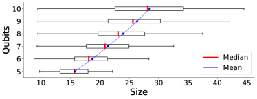
(c)

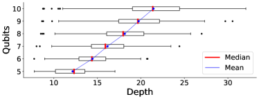
(d)

Figure 5: Different metrics for the generated test patterns. The evaluation is based on QFT circuits and the circuit sizes range from 5 qubits to 10 qubits. The box extends from the first quartile to the third quartile of the data.

TABLE II: Averaged metric values of the generated test patterns on different benchmark circuits. The numbers in parentheses represent the optimal circuit size (depth) if we carefully choose the initial subspace $Q$ (see Equation (6)).

	$\nu^{*}(\mathcal{A}_{\rho})$	$\nu(\mathcal{B}_{M})$	Sparsity	Size	Depth
QFT_5	1.698	3.381	84.0	15.7	12.2
QFT_6	1.956	4.056	171.5	18.7	14.4
QFT_7	2.272	4.764	338.4	21.4	16.2
QFT_8	2.653	5.484	624.8	24.0	18.1
QFT_9	3.112	6.222	1004.7	26.3	19.7
QFT_10	3.736	6.938	1390.8	28.5	21.4
QV_5	2.119	8.632	835.0	26.8	19.2
QV_7	3.209	15.006	5118.4	33.3	22.8
BV_10	1.493	1.479	10.3	18.9	15.9
BV_100	1.513	1.497	10.6	162.0 (37)	145.2 (7)

In this section, we apply the proposed SPD generation algorithm on different benchmark circuits and evaluate the generated test patterns. First, an illustrative example is shown in Fig. 4. In this example, the SPD generation algorithm is applied on the 3-qubit QFT circuit (see sub-figure (a)), where the middle red-colored $R_{z}(\pi/4)$ gate is suspected to be faulty. Two different fault models are adopted and the corresponding test patterns are generated respectively. The sub-figures (b)-(h) are test patterns for the missing-gate fault, and the sub-figures (i)-(v) are test patterns for the replaced-by-$R_{X}(\pi/3)$ fault. The number and signed Pauli operators in the caption of each sub-figures (excluding sub-figure (a)) represent the coefficient and corresponding stabilizer projector of the SPD. The test patterns that have input (output) labels are input (output) patterns. The input labels represent the specified input, and those qubits without input labels are in the maximally mixed state. The output labels represent the specified measurement output, and those qubits without output labels are simply discarded.

We then evaluate the performance of the proposed SPD generation algorithm in detail. Specifically, we are concerned with the following metrics: 1) the product of the SPD 1-norm $\nu^{*}(\mathcal{A}_{\rho})\nu(\mathcal{B}_{M})$, where $\mathcal{A}_{\rho}$ denotes the generated SPD for test input $\rho$ and $\mathcal{B}_{M}$ denotes the generated SPD for test measurement $M$, 2) the sparsity of the generated SPD, 3) the size of the quantum Clifford circuit that implements the test pattern, and 4) the depth of the quantum Clifford circuit that implements the test pattern. The first metric $\nu^{*}(\mathcal{A}_{\rho})\nu(\mathcal{B}_{M})$ could be treated as a quantity that measures how “non-Clifford” the SPD is. It heavily impacts the iteration number needed in the sampling algorithm (see Algorithm 1). The second metric reflects the computational complexity required for any non-trivial operation on the SPD. The third and fourth metrics reflect the complexity of the Clifford circuit implementing the test patterns.

First, we conduct the experiments on QFT circuits with the sizes ranging from 5 qubits to 10 qubits. For each potential fault in the circuit, the corresponding test patterns (represented by SPD) are generated by our algorithm, and then evaluated with the aforementioned metrics. The results are shown in Fig. 5. It is worth noting that, though the maximum of $\nu^{*}(\mathcal{A}_{\rho})\nu(\mathcal{B}_{M})$ grows rapidly, the median of $\nu^{*}(\mathcal{A}_{\rho})\nu(\mathcal{B}_{M})$ grows slowly with the number of qubits. This demonstrates good scalability of the SPD in a considerable proportion of the cases. Similarly, the median of sparsity scales moderately compared to its maximum value, which demonstrates the computational efficiency of the SPD generation in the average sense. We believe that the SPD generation algorithm can be further accelerated using advanced parallel techniques on classical computer. We also observe that the averaged circuit size and depth of the test pattern scale almost linearly, which further ensures the practical feasibility of the proposed test application scheme. Then, we also evaluate the QV and BV circuits, where the results are shown in Table II. Note that for the 7-qubit QV circuit, the metrics $\nu^{*}(\mathcal{A}_{\rho})$, $\nu(\mathcal{B}_{M})$ and the sparsity are rather higher than others. This is likely because QV is a kind of randomized quantum circuits designed for quantifying the maximal capacity of a quantum device, so that it is much more complicated than most of the quantum circuits for normal uses. In contrast, the BV circuit contains only Clifford gates, so that our algorithm even scales well for the circuit size up to 100 qubits.

V-C Test Application and Fault Detection

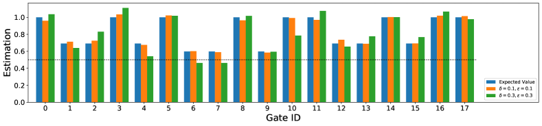
Figure 6: An illustrative example for the sampling algorithm (Algorithm 1) on 3-qubit QFT circuit. The orange and green bars represent the simulation results with different parameters, and the blue bar represents the expected output. The gate ID $i$ means that we apply the test patterns for the $i$-th gate.

TABLE III: Simulation results for quantum fault detection.

	TP	TN	FP	FN	Prec.	Rec.	Acc.
QV_5	51	49	0	0	1.0	1.0	1.0
BV_10	47	53	0	0	1.0	1.0	1.0
QFT_5	46	47	7	0	0.87	1.0	0.93
QFT_10	44	47	9	0	0.83	1.0	0.91

In this section, we apply the previously generated test patterns on benchmark circuits by simulating the sampling algorithm (Algorithm 1). Then, we show the overall results of our framework for quantum circuit fault detection. First, an illustrative example is shown in Fig. 6. In this example, we simulate the sampling algorithm on the 3-qubit fault-free QFT circuit, using the test pattern for each gate in the circuit. The orange and green bars represent the simulation results with different parameters, and the blue bar represents its expected value. The gate ID $i$ indicates that the result is from applying the test patterns of $i$-th gate. First note that when setting $\delta=0.1,\epsilon=0.1$, the estimation returned by the sampling algorithm successfully approximates the ideal output. We found that when applying the test patterns of gate 6 and gate 7, the green bar is lower than $0.5$. This means we may misclassify the CUT as faulty circuit when we set the classification threshold to be $0.5$, resulting in a false positive alert. However, this is mainly because the gate itself is close to the identity gate to some extent. Thus it is intrinsically difficult to detect such fault under the SMGF (single missing gate fault) model. Except gate-6 and gate-7, there is no big difference between the results of using parameters $\delta=0.1,\epsilon=0.1$ and $\delta=0.3,\epsilon=0.3$ while the latter one requires fewer iterations. This means if the faults are sufficiently distinguishable, then the parameters $\delta=0.3,\epsilon=0.3$ may be a practical choice that are both efficient and sound.

Then we evaluate our algorithms for the fault detection task. We first randomly selected $k$ candidate fault-sites in the benchmark circuit such that the maximal discrimination probability is at least $0.5+\tau$. This is because the discrimination probability of $0.5+\tau$ indicates that the trace distance between fault-free and faulty output is at most $2\tau$. Thus $\tau\rightarrow 0$ indicates that the fault is negligible and inherently hard to detect. With the probability of $0.5$, the CUT is set to be faulty, and otherwise the CUT is set to be fault-free. When the CUT is faulty, a fault-site is randomly selected from the $k$ candidates and the gate at the fault-site is replaced by its faulty version. For each candidate fault-site $i$, the corresponding test patterns are automatically generated and applied on the CUT by simulating the sampling algorithm (with parameters $\epsilon,\delta$) to obtain the estimation $m_{i}$. The CUT is predicted to be faulty if $\min\{m_{1},\ldots,m_{k}\}\leq 0.5$, and otherwise is predicted to be fault-free. Note that we need to correctly obtain $k$ estimations to ensure that the final prediction is correct. Since the parameter $\epsilon$ bounds the success probability of our sampling algorithm from below, we set this parameter to $\epsilon/k$ to ensure that the overall success probability for fault detection is at least $1-\epsilon$. Note that the complexity of our sampling algorithm scales logarithmically with $1/\epsilon$, thus the overhead is still acceptable. In this work, we set $k=10,\tau=0.1,\delta=0.3,\epsilon=0.3$. For each benchmark circuit, we repeat the above fault detection procedure $100$ times and the experimental results are shown in Table III.

Our method achieves the highest recall (1.0) uniformly in all experiments, which means all the faults in the quantum circuits are detected with success probability $1.0$. We also found that there are some false positive alerts in the experiments for QFT_5 and QFT_10 circuits, i.e., some fault-free circuits are misclassified as faulty circuits. However, the precision is still higher than $0.83$ and the false positive rate (FPR) is lower than $0.16$. Furthermore, since the recall is sufficiently close to $1.0$, the false positive alerts can be effectively eliminated by repeating the test on the false positive samples and excluding the samples once they are classified as negative (i.e., fault-free). Finally, the overall performance of fault detection is much better than expected by the theoretical bounds (failure probability $\epsilon=0.3$ and estimation deviation $\delta=0.3$), which indicates rather good performance of our method in practice.

VI Conclusion

In this paper, we propose a new ATPG framework for robust quantum circuit testing. The stabilizer projector decomposition (SPD) is introduced for representing the quantum test pattern, and an SPD generation algorithm is developed. Furthermore, the test application is reconstructed using Clifford-only circuits with classical randomness. To tackle the issue of exponentially growing size of the involved optimization problem, we proposed several acceleration techniques that can exploit both locality and sparsity in SPD generation. It is proved that the locality exploiting algorithm will return optimal result under some reasonable conditions. To demonstrate the effectiveness and efficiency, the overall framework is implemented and evaluated on several commonly used benchmark circuits.

For future research, we plan to extend our work in the following two directions:

VI-1 Adaptive quantum ATPG

The adaptive ATPG method [36] for classical circuits utilizes the existing output responses from the CUT to guide the automatic generation of new test patterns, which makes the fault diagnosis much more efficient. In the quantum case, however, the output responses are quantum states, and thus we cannot easily make use of the information in the output responses due to the high cost of quantum state tomography. Further, the response analysis and pattern generation guidance are much more complicated than those for classical circuit. These make the development of adaptive quantum ATPG high nontrivial.

VI-2 Different Fault Models and Circuit Models

In this paper, we assume that the faulty gate is still a unitary gate. This assumption does cover some important classes of faults in the real-world applications. But in many applications, in particular in the current NISQ (Noisy Intermediate Scale Quantum) era, a fault gate is often a non-unitary gate. Then techniques for discriminating a unitary gate and a general quantum operation (see e.g. [37]) is vital in ATPG for this kind of faults. On the other hand, we only consider combinational quantum circuits in this paper. Recently, several new circuit models have been introduced in quantum computing and quantum information. One interesting model is dynamic quantum circuits (see e.g. [38, 39]) in which quantum measurements can occur at the middle of the circuits and the measurement outcomes are used to conditionally control subsequent steps of the computation. A fault in these circuits may happen not only at a quantum gate but also at a measurement. Therefore, techniques for discriminating quantum measurements (see e.g. [40]) will be needed in ATPG for them. Another interesting model is sequential quantum circuits [41]. As we know, in the classical case, ATPG for combinational circuits and that for sequential ones are fundamentally different. The quantum case is similar, and the approach presented in this paper cannot directly generalised to sequential quantum circuits.

Appendix

In this appendix, we provide the detailed proofs of all lemmas, propositions and theorems omitted in the main body of the paper.

VI-A Minimal Norms of SPD

Definition 3 (Minimal SPD norms).

The minimal 1-norm $\xi$ and minimal weighted 1-norm $\xi^{*}$ of operator $A$ are defined by

$$\small\begin{gathered}\xi(A)=\min\bigg{\{}\nu(\mathcal{A})\;\bigg{|}\;\mathcal{A}\in\textup{SPD}(A)\bigg{\}}\\ \xi^{*}(A)=\min\bigg{\{}\nu^{*}(\mathcal{A})\;\bigg{|}\;\mathcal{A}\in\textup{SPD}(A)\bigg{\}}\end{gathered}$$ (28)

We say that $\mathcal{A}$ is $\nu$-optimal (respectively, $\nu^{*}$-optimal) for $A$ if $\mathcal{A}\in\textup{SPD}(A)$ and $\nu(\mathcal{A})=\xi(A)$ (respectively, $\nu^{*}(\mathcal{A})=\xi^{*}(A)$).

The above definition is a generalization of the robustness of magic in quantum resource theory [24]. Some basic properties of $\xi$ and $\xi^{*}$ are given in the following:

Proposition 2.

Both $\xi$ and $\xi^{*}$ are invariant under applying Clifford unitary and tensoring stabilizer projector:

1. Clifford Invariance: for any Clifford unitary $U$,

   $$\xi(UAU^{\dagger})=\xi(A),\quad\xi^{*}(UAU^{\dagger})=\xi^{*}(A).$$

2. Tensor Invariance: for any stabilizer projector $A$,

   $$\xi(A\otimes B)=\xi(B),\quad\xi^{*}(A\otimes B)=\textup{tr}A\cdot\xi^{*}(B).$$

The Clifford invariance is obvious and the proof of tensor invariance is given in the next section.

VI-B Proof of Proposition 2 (Tensor Invariance)

The proof of Proposition 2 requires several technical lemmas:

Lemma 2.

Suppose $A$ is a stabilizer projector of bipartite system $ST$, where $S$ is a single qubit subsystem. Then

$$\langle 0|A|0\rangle=cB$$ (29)

where $B$ is a stabilizer projector of $T$ and $0\leq c\leq 1$. Furthermore, if $c=1$, then $A\sqsupseteq|0\rangle\!\langle 0|\otimes B$.

Proof.

Suppose $G=\langle P_{1},\ldots,P_{l}\rangle$ is the signed Pauli group associated to the stabilizer projector $A$ where $P_{1},\ldots,P_{l}$ are independent generators of $G$. Without loss of generality, we can assume that either $Z_{1}$ commutes with all $P_{i}$ or only anti-commutes with $P_{l}$.

If $Z_{1}$ commutes with all $P_{i}$, then

$$\begin{split}|0\rangle\!\langle 0|\otimes cB&=|0\rangle\!\langle 0|A|0\rangle\!\langle 0|\\ &=\frac{I+Z_{1}}{2}A\frac{I+Z_{1}}{2}\\ &=\frac{I+Z_{1}}{2}\prod_{i\leq l}\frac{I+P_{i}}{2}\frac{I+Z_{1}}{2}\\ &=\prod_{i\leq l}\frac{I+P_{i}}{2}\frac{I+Z_{1}}{2}\end{split}$$ (30)

Since each $P_{i}$ commutes with $Z_{1}$, $\langle P_{1},\ldots,P_{l},Z_{1}\rangle$ is a stabilizer group. Thus we can replace $P_{i}$ by $P_{i}Z_{1}$ (if necessary) to ensure that $P_{i}$ is of the form $I\otimes P^{\prime}_{i}$. This means

$$|0\rangle\!\langle 0|\otimes cB=|0\rangle\!\langle 0|\otimes\prod_{i\leq l}\frac{I+P^{\prime}_{i}}{2}$$ (31)

Thus $c=1$ and $B$ is a stabilizer projector.

If $Z_{1}$ anti-commutes with $P_{l}$, then

$$\begin{split}|0\rangle\!\langle 0|\otimes cB&=|0\rangle\!\langle 0|A|0\rangle\!\langle 0|\\ &=\frac{I+Z_{1}}{2}A\frac{I+Z_{1}}{2}\\ &=\prod_{i\leq l-1}\frac{I+P_{i}}{2}\frac{I+Z_{1}}{2}\frac{I+P_{l}}{2}\frac{I+Z_{1}}{2}\\ &=\frac{1}{2}\prod_{i\leq l-1}\frac{I+P_{i}}{2}\frac{I+Z_{1}}{2}\end{split}$$ (32)

Similarly, we can assume $P_{i}$ is of the form $I\otimes P^{\prime}_{i}$, which means

$$|0\rangle\!\langle 0|\otimes cB=|0\rangle\!\langle 0|\otimes\frac{1}{2}\prod_{i\leq l-1}\frac{I+P^{\prime}_{i}}{2}$$ (33)

Thus $c=1/2$ and $B$ is a stabilizer projector.

Furthermore, $c=1$ indicates that all $P_{i}$ commutes with $Z_{1}$. So each $P_{i}$ is either of the form $I\otimes P^{\prime}_{i}$ or of the form $Z\otimes P^{\prime}_{i}$. If $P_{i}=I\otimes P^{\prime}_{i}$ for all $i$, then

$$A=I\otimes\prod\frac{I+P^{\prime}_{i}}{2}=I\otimes B\sqsupseteq|0\rangle\!\langle 0|\otimes B$$ (34)

Otherwise, there is some generator $P_{i}=Z\otimes P^{\prime}_{i}$. Without loss of generality, we can assume that only $P_{l}$ has the form $Z\otimes P^{\prime}_{l}$. Then

$$\begin{split}A&=(I\otimes\prod_{i<l}\frac{I+P^{\prime}_{i}}{2})\frac{I+Z\otimes P^{\prime}_{l}}{2}\\ &=(I\otimes\prod_{i<l}\frac{I+P^{\prime}_{i}}{2})\big{(}|0\rangle\!\langle 0|\otimes\frac{I+P^{\prime}_{l}}{2}+|1\rangle\!\langle 1|\otimes\frac{I-P^{\prime}_{l}}{2}\big{)}\\ &=|0\rangle\!\langle 0|\otimes\prod_{i\leq l}\frac{I+P^{\prime}_{i}}{2}+|1\rangle\!\langle 1|\otimes\prod_{i<l}\frac{I+P^{\prime}_{i}}{2}\frac{I-P^{\prime}_{l}}{2}\\ &\sqsupseteq|0\rangle\!\langle 0|\otimes B\end{split}$$

∎

Lemma 3.

Suppose $A$ is a stabilizer projector of bipartite system $ST$, where $S$ is an $n$-qubit system, then

$$\langle 0|^{\otimes n}A|0\rangle^{\otimes n}=cB$$ (35)

where $B$ is a stabilizer projector of $T$ and $0\leq c\leq 1$. Furthermore, if $c=1$, then $A\sqsupseteq|0\rangle\!\langle 0|^{\otimes n}\otimes B$

Proof.

By inductively apply Lemma 2. ∎

Lemma 4.

Suppose $A$ is a stabilizer projector of bipartite system $ST$, then

$$\textup{tr}_{S}(A)=cB$$ (36)

where $B$ is a stabilizer projector and $0\leq c\leq\dim(S)$. Furthermore, if $c=\dim(S)$, then $A=I\otimes B$.

Proof.

Suppose $G=\{P_{i}\}_{i}$ is the stabilizer group associated to the stabilizer projector $A$. Obviously, all the signed Pauli operators $P_{i}$ that act trivially on system $T$ (i.e., $P_{i}=I\otimes P^{\prime}_{i}$) form a subgroup $G^{\prime}$. Then,

$$\begin{split}\textup{tr}_{S}(A)&=\frac{1}{|G|}\sum_{P_{i}\in G}\textup{tr}_{S}(P_{i})\\ &=\frac{1}{|G|}\sum_{P_{i}\in G^{\prime}}\textup{tr}_{S}(P_{i})\\ &=\frac{\dim(S)}{|G|}\sum_{P_{i}\in G^{\prime}}P^{\prime}_{i}\\ &=\frac{\dim(S)|G^{\prime}|}{|G|}\frac{1}{|G^{\prime}|}\sum_{P_{i}\in G^{\prime}}P^{\prime}_{i}\\ &=\frac{\dim(S)|G^{\prime}|}{|G|}B\end{split}$$ (37)

So $c=\dim(S)|G^{\prime}|/|G|\leq\dim(S)$ and $B$ is a stabilizer projector. Furthermore, if $c=\dim(S)$, then $|G^{\prime}|=|G|$. This means $G^{\prime}=G$ and thus $P_{i}=I\otimes P^{\prime}_{i}$ for all $P_{i}\in G$. So $A=I\otimes B$. ∎

Now we are ready to give the proof of Proposition 2. For the clarity, let us split the proposition into the following two:

Proposition 3 (Tensor Invariance of $\xi$).

$$\xi(A\otimes B)=\xi(B)$$ (38)

where $A$ is a stabilizer projector.

Proof.

We use $S$ and $T$ to denote the subsystems corresponding to the operators $A$ and $B$ respectively. By Corollary 1, there is a Clifford unitary $U$ such that $UAU^{\dagger}=|0\rangle\!\langle 0|^{\otimes m}\otimes I_{n}$, where $m=\log\dim(S)-\log\textup{tr}(A)$ and $n=\log\textup{tr}(A)$. Suppose $\{(a_{i},A_{i})\}$ is an optimal SPD for $|0\rangle\!\langle 0|^{\otimes m}\otimes I_{n}\otimes B$, so

$$|0\rangle\!\langle 0|^{\otimes m}\otimes I_{n}\otimes B=\sum_{i}a_{i}A_{i}$$ (39)

By Lemma 3

$$\begin{split}I_{n}\otimes B=\sum_{i}a_{i}\langle 0|^{\otimes m}A_{i}|0\rangle^{\otimes m}=c_{1}\sum_{i}a_{i}A^{\prime}_{i}\end{split}$$ (40)

where $0\leq c_{1}\leq 1$ and $A^{\prime}_{i}$ are stabilizer projectors. By Lemma 4

$$\begin{gathered}2^{n}\cdot B=c_{1}\sum_{i}a_{i}\textup{tr}_{n}(A^{\prime}_{i})=c_{1}c_{2}\sum_{i}a_{i}A^{\prime\prime}_{i}\end{gathered}$$ (41)

where $0\leq c_{2}\leq 2^{n}$, $\textup{tr}_{n}$ denotes the partial trace on first $n$ quibts and $A^{\prime\prime}_{i}$ are stabilizer projectors. Thus

$$B=c_{1}\cdot c_{2}/2^{n}\cdot\sum_{i}a_{i}A^{\prime\prime}_{i}$$ (42)

This implies $\xi(B)\leq\xi(|0\rangle\!\langle 0|^{\otimes m}\otimes I_{n}\otimes B)=\xi(A\otimes B)$. But obviously we have $\xi(A\otimes B)\leq\xi(B)$. Thus $\xi(A\otimes B)=\xi(B)$. ∎

Proposition 4 (Tensor Invariance of $\xi^{*}$).

$$\xi^{*}(A\otimes B)=\textup{tr}A\cdot\xi^{*}(B)$$ (43)

where $A$ is a stabilizer projector.

Proof.

Since any stabilizer projector $S$ can be expanded into the sum of $\textup{tr}S$ stabilizer states, we can show that there is an stabilizer state decomposition

$$A\otimes B=\sum_{i}a_{i}\sigma_{i}$$ (44)

where $\sigma_{i}$ are stabilizer states and $\sum_{i}|a_{i}|=\xi^{*}(A\otimes B)$. We use $S$ to denote the subsystem of operator $A$. By Lemma 4

$$\begin{gathered}\textup{tr}A\cdot B=\sum_{i}a_{i}\textup{tr}_{S}(\sigma_{i})=\sum_{i}a_{i}c_{i}\sigma^{\prime}_{i}\end{gathered}$$ (45)

where $\sigma^{\prime}_{i}$ are stabilizer projectors and $c_{i}\textup{tr}(\sigma^{\prime}_{i})=\textup{tr}(\sigma_{i})=1$. This means

$$B=\sum_{i}a_{i}\frac{1}{\textup{tr}A\cdot\textup{tr}(\sigma^{\prime}_{i})}\sigma^{\prime}_{i}$$ (46)

This implies $\xi^{*}(B)\leq 1/\textup{tr}A\cdot\sum_{i}|a_{i}|=1/\textup{tr}A\cdot\xi^{*}(A\otimes B)$. But obviously we have $\xi^{*}(A\otimes B)\leq\textup{tr}(A)\xi^{*}(B)$. Thus $\xi^{*}(A\otimes B)=\textup{tr}A\cdot\xi^{*}(B)$ ∎

VI-C Proof of Theorem 2 (Optimality of Algorithm 3)

First, we show that the SPD is in a canonical form if one of the two conditions in Theorem 2 is satisfied. For clarity, we will prove the two cases separately.

Proposition 5.

Suppose $A$ is a stabilizer projector and $B$ is a positive operator. If $\mathcal{C}=\{(c_{i},C_{i})\}\in\textup{SPD}(A\otimes B)$ satisfies

1. $\mathcal{C}$ is $\nu$-optimal,

2. $\mathcal{C}$ has the smallest $\nu^{*}$ among all $\nu$-optimal SPDs of $A\otimes B$

then each $C_{i}$ has the form $C_{i}=A\otimes C^{\prime}_{i}$

Proof.

Suppose $A$ is an $n$-qubit stabilizer projector and let $m=\log\textup{tr}A$. Then, there is a Clifford unitary $U$ such that $UAU^{\dagger}=|0\rangle\!\langle 0|^{\otimes n-m}\otimes I_{m}$, where $I_{m}$ is the identity operator on the $m$-qubit system. Note that $U$ is Clifford, if $\{(c_{i},C_{i})\}$ satisfies conditions 1) and 2) for $A\otimes B$, then $\{(c_{i},UC_{i}U^{\dagger})\}$ also satisfies conditions 1) and 2) for $UAU^{\dagger}\otimes B$. This means we only need to prove this proposition with $A=|0\rangle\!\langle 0|^{n-m}\otimes I_{m}$ where $m\geq 0$.

First, note that

$$\begin{split}\sum_{i}c_{i}\langle 0|^{\otimes n-m}C_{i}|0\rangle^{\otimes n-m}&=\langle 0|^{\otimes n-m}A\otimes B|0\rangle^{\otimes n-m}\\ &=I_{m}\otimes B\end{split}$$ (47)

By Lemma 3, $c_{i}\langle 0|^{\otimes n-m}C_{i}|0\rangle^{\otimes n-m}=c^{\prime}_{i}C^{\prime}_{i}$ where $|c^{\prime}_{i}|\leq|c_{i}|$ and $C^{\prime}_{i}$ are also stabilizer projectors. This means

$$\xi(I_{m}\otimes B)\leq\sum_{i}|c^{\prime}_{i}|\leq\sum_{i}|c_{i}|=\xi(A\otimes B)$$ (48)

However, by the tensor invariance of $\xi$, i.e.,

$$\xi(A\otimes B)=\xi(|0\rangle\!\langle 0|^{\otimes n-m}\otimes I_{m}\otimes B)=\xi(I_{m}\otimes B),$$

we can conclude that $c_{i}=c^{\prime}_{i}$. This means each $C_{i}$ satisfies $C_{i}\sqsupseteq|0\rangle\!\langle 0|^{\otimes n-m}\otimes C^{\prime}_{i}$ (see Lemma 3). Note that $\{(c_{i},|0\rangle\!\langle 0|^{\otimes n-m}\otimes C^{\prime}_{i})\}$ is also a $\nu$-optimal SPD for $A\otimes B$ since

$$\sum_{i}c_{i}|0\rangle\!\langle 0|^{\otimes n-m}\otimes C^{\prime}_{i}=|0\rangle\!\langle 0|^{\otimes n-m}\otimes I_{m}\otimes B$$ (49)

and has smaller $\nu^{*}$, i.e.,

$$\sum_{i}|c_{i}|\textup{tr}(|0\rangle\!\langle 0|^{\otimes n-m}\otimes C^{\prime}_{i})\leq\sum_{i}|c_{i}|\textup{tr}(C_{i})$$ (50)

So by condition 2), we conclude that $C_{i}=|0\rangle\!\langle 0|^{\otimes n-m}\otimes C^{\prime}_{i}$.

Next,

$$\begin{split}2^{m}\cdot B&=\textup{tr}_{m}(I_{m}\otimes B)=\textup{tr}_{m}(\sum_{i}c_{i}C^{\prime}_{i})\\ &=\sum_{i}c_{i}\textup{tr}_{m}(C^{\prime}_{i})\end{split}$$ (51)

where $\textup{tr}_{m}$ denotes the partial trace for the system of first $m$ qubits. By Lemma 4, $c_{i}\textup{tr}_{m}(C^{\prime}_{i})=2^{m}c^{\prime\prime}_{i}C^{\prime\prime}_{i}$, where $|c^{\prime\prime}_{i}|\leq|c_{i}|$ and $C^{\prime\prime}_{i}$ are also stabilizer projectors. Thus $B=\sum_{i}c^{\prime\prime}_{i}C^{\prime\prime}_{i}$ and

$$\xi(B)\leq\sum_{i}|c^{\prime\prime}_{i}|\leq\sum_{i}|c_{i}|=\xi(A\otimes B).$$

Similarly, by the tensor invariance of $\xi$, we can conclude that $c^{\prime\prime}_{i}=c_{i}$. This means each $C^{\prime}_{i}$ has the form $C^{\prime}_{i}=I_{m}\otimes C^{\prime\prime}_{i}$ (see Lemma 4). So,

$$C_{i}=|0\rangle\!\langle 0|^{\otimes n-m}\otimes I_{m}\otimes C^{\prime\prime}_{i}=A\otimes C^{\prime\prime}_{i}.$$

∎

Proposition 6.

Suppose $A$ is a stabilizer projector and $B$ is a positive operator. If $\mathcal{C}=\{(c_{i},C_{i})\}\in\textup{SPD}(A\otimes B)$ satisfies

1. $\mathcal{C}$ is $\nu^{*}$-optimal,

2. $\mathcal{C}$ has the smallest $\nu$ among all $\nu^{*}$-optimal SPDs of $A\otimes B$

then each $C_{i}$ has the form $C_{i}=A\otimes C^{\prime}_{i}$

Proof.

Suppose $A$ is an $n$-qubit stabilizer projector and let $m=\log\textup{tr}A$. Similarly, we only need to prove this proposition with $A=|0\rangle\!\langle 0|^{n-m}\otimes I_{m}$ where $m\geq 0$.

First, note that

$$\begin{split}\sum_{i}c_{i}\langle 0|^{\otimes n-m}C_{i}|0\rangle^{\otimes n-m}&=\langle 0|^{\otimes n-m}A\otimes B|0\rangle^{\otimes n-m}\\ &=I_{m}\otimes B\end{split}$$ (52)

By Lemma 3, $c_{i}\langle 0|^{\otimes n-m}C_{i}|0\rangle^{\otimes n-m}=c^{\prime}_{i}C^{\prime}_{i}$ where $C^{\prime}_{i}$ are stabilizer projectors. Note that

$$\begin{split}\textup{tr}C_{i}&=\sum_{j\in\{0,1\}^{n-m}}\textup{tr}\langle j|C_{i}|j\rangle\\ &\geq\textup{tr}\langle 0|^{\otimes n-m}C_{i}|0\rangle^{\otimes n-m}\\ &=\frac{c^{\prime}_{i}}{c_{i}}\textup{tr}C^{\prime}_{i}\end{split}$$ (53)

which means $|c_{i}|\textup{tr}C_{i}\geq|c^{\prime}_{i}|\textup{tr}C^{\prime}_{i}$. Then, we have

$$\xi^{*}(I_{m}\otimes B)\leq\sum_{i}|c^{\prime}_{i}|\textup{tr}C^{\prime}_{i}\leq\sum_{i}|c_{i}|\textup{tr}C_{i}=\xi^{*}(A\otimes B)$$ (54)

However, by the tensor invariance of $\xi^{*}$, i.e.,

$$\xi^{*}(A\otimes B)=\xi^{*}(|0\rangle\!\langle 0|^{\otimes n-m}\otimes I_{m}\otimes B)=\xi^{*}(I_{m}\otimes B).$$

We can conclude that $c_{i}\textup{tr}C_{i}=c^{\prime}_{i}\textup{tr}C^{\prime}_{i}$ and so that $\langle j|C_{i}|j\rangle=0$ for all $0^{n-m}\neq j\in\{0,1\}^{n-m}$. This means $C_{i}=|0\rangle\!\langle 0|^{\otimes n-m}\otimes C^{\prime}_{i}$.

Next, we have:

$$\begin{split}2^{m}\cdot B&=\textup{tr}_{m}(I_{m}\otimes B)=\textup{tr}_{m}(\sum_{i}c_{i}C^{\prime}_{i})\\ &=\sum_{i}c_{i}\textup{tr}_{m}(C^{\prime}_{i})\end{split}$$ (55)

where $\textup{tr}_{m}$ denotes the partial trace for the system of first $m$ qubits. By Lemma 4, $c_{i}\textup{tr}_{m}(C^{\prime}_{i})=2^{m}c^{\prime\prime}_{i}C^{\prime\prime}_{i}$, where $|c^{\prime\prime}_{i}|\leq|c_{i}|$ and $C^{\prime\prime}_{i}$ are also stabilizer projectors. Thus $B=\sum_{i}c^{\prime\prime}_{i}C^{\prime\prime}_{i}$ and $I_{m}\otimes B=\sum_{i}c^{\prime\prime}_{i}I_{m}\otimes C^{\prime\prime}_{i}$. Note that

$$\begin{gathered}\sum_{i}|c^{\prime\prime}_{i}|2^{m}\textup{tr}(C^{\prime\prime}_{i})=\sum_{i}|c_{i}|\textup{tr}(C^{\prime}_{i})=\xi(I_{m}\otimes B)\end{gathered}$$ (56)

which means $\{(c^{\prime\prime}_{i},I_{m}\otimes C^{\prime\prime}_{i})\}$ is a $\nu^{*}$-optimal SPD for $I_{m}\otimes B$. It also has smaller $\nu$, i.e.,

$$\sum_{i}|c^{\prime\prime}_{i}|\leq\sum_{i}|c_{i}|$$ (57)

So by condition 2), we have $|c^{\prime\prime}_{i}|=|c_{i}|$, and thus $C^{\prime}_{i}=I_{m}\otimes C^{\prime\prime}_{i}$ (see Lemma 4).

So, $C_{i}=|0\rangle\!\langle 0|^{\otimes n-m}\otimes I_{m}\otimes C^{\prime\prime}_{i}=A\otimes C^{\prime\prime}_{i}$. ∎

Then, we are ready to prove Theorem 2. We will first prove the correctness (i.e., the output of Algorithm 3 correctly reveal the locality) and then prove its optimality.

Proof of Theorem 2.

Correctness: First we prove the correctness of Algorithm 3. Note that $V_{1}$ maps $\hat{P}_{1},\ldots,\hat{P}_{l},P_{U}$ to $Z_{1},\ldots,Z_{l},Z_{l+1}$. This means the group $V_{1}G_{i}V_{1}^{\dagger}$ can be generated by $Z_{1},\ldots,Z_{l},\tilde{P}_{i,1}\otimes P_{i,1},\ldots,\tilde{P}_{i,l_{i}}\otimes P_{i,l_{i}}$, where $\tilde{P}_{i,j}$ are Pauli operators on first $l$ qubits. Note that $\tilde{P}_{i,j}$ contains only $I$ and $Z$, as $\tilde{P}_{i,j}$ commutes with all $Z_{1},\ldots,Z_{l}$. We can set $\tilde{P}_{i,j}$ to $I_{l}$ by multiplying several $Z_{k},k\leq l$ if necessary. Thus each $V_{1}G_{i}V_{1}^{\dagger}$ has the generators $Z_{1},\ldots,Z_{l},I_{l}\otimes P_{i,1},\ldots,I_{l}\otimes P_{i,l_{i}}$, which means $V_{1}A_{i}V_{1}^{\dagger}=|0\rangle\!\langle 0|^{\otimes l}\otimes A^{\prime}_{i}$ where

$$A^{\prime}_{i}=\prod_{j\leq l_{i}}\frac{I+P_{i,j}}{2}.$$

Besides, it holds that

$$V_{1}UV_{1}^{\dagger}=V_{1}e^{i\theta P_{U}}V_{1}^{\dagger}=e^{i\theta Z_{l+1}}=I_{l}\otimes e^{i\theta Z_{1}}.$$

Consider the subsystem that excludes the first $l$ qubits. By steps 10-17 of Algorithm 3, we can ensure that each $Q_{i}$ at most anti-commutes with one $Q_{j}$. Then, by exchanging the subscripts, we can make $\{Q_{i}\}$ normal, i.e., $\exists t$ such that $Q_{1},\ldots,Q_{t}$ commute with all $Q_{i}$ for $i\leq s$ and $Q_{t+2i-1}$ only anti-commutes with $Q_{t+2i}$ for $i=1,\ldots,(s-t)/2$. Then, we can find a Clifford unitary $V_{2}$ that maps $\{Q_{1},\ldots,Q_{t}\}$ to $\{Z_{1},\ldots,Z_{t}\}$ and maps $\{Q_{t+1},\ldots,Q_{s}\}$ to $\{Z_{t+1},X_{t+1},\ldots,Z_{(t+s)/2},X_{(t+s)/2}\}$ (see Lemma 1). Since $\{Q_{1},\ldots,Q_{s}\}$ is the maximal independent set, $V_{2}$ transforms all $P_{i,j}$ and $Z_{1}$ to the signed Pauli operators of the form $I_{n^{\prime}-(s+t)/2}\otimes P$ where $P$ acts on a subsystem of size $(s+t)/2$. Thus,

$$V_{2}A^{\prime}_{i}V_{2}^{\dagger}=I_{n^{\prime}-(s+t)/2}\otimes A^{\prime\prime}_{i}$$

for all $i$ and

$$V_{2}U^{\prime}V_{2}^{\dagger}=I_{n^{\prime}-(s+t)/2}\otimes U^{\prime\prime},$$

where $A^{\prime\prime}_{i}$ and $U^{\prime\prime}$ are the stabilizer projectors and non-Clifford unitary in a subsystem of size $(t+s)/2$. Note that $V=V_{2}V_{1}$ is then the required unitary, i.e.,

$$VUV^{\dagger} =I_{n-(s+t)/2}\otimes U^{\prime\prime}$$

$$VA_{i}V^{\dagger} =|0\rangle\!\langle 0|^{\otimes l}\otimes I_{n^{\prime}-(s+t)/2}\otimes A^{\prime\prime}_{i}.$$

Optimality: Then we prove the optimality of Algorithm 3. Suppose the optimal Clifford unitary is $\overline{V}$ which satisfies $\overline{V}A\overline{V}^{\dagger}=B\otimes\overline{A}$ and $\overline{V}U\overline{V}^{\dagger}=W\otimes\overline{U}$, where $B$ is a stabilizer projector, $W$ is a Clifford unitary and $\overline{A},\overline{U}$ act in a subsystem of size $\overline{n}$. Without loss of generality, we can assume that $B=|0\rangle\!\langle 0|^{\otimes l}\otimes I_{n-\overline{n}-l}$ (by applying extra Clifford unitary on $B$). By conditions 1), 2) and Proposition 5 and 6, we know that for each $A_{i}$, it can be written as follows:

$$A_{i}=\overline{V}^{\dagger}(|0\rangle\!\langle 0|^{\otimes l}\otimes I\otimes\overline{A}_{i})\overline{V}$$ (58)

where $\overline{A}_{i}$ are stabilizer projectors. For convenience, we denote $I_{n-\overline{n}-l}\otimes\overline{A}_{i}$ as $\tilde{A}_{i}$.

Besides, $W\otimes\overline{U}$ is of the form $I_{n-\overline{n}}\otimes e^{i\theta\overline{P}_{U}}$. This is because $e^{i\theta P_{U}}=U=\overline{V}^{\dagger}(W\otimes\overline{U})\overline{V}$ has two different eigenvalues (here we do not consider multiplicity of eigenvalues), which means $W$ and $\overline{U}$ at most have two different eigenvalues. As $\overline{U}$ is a non-Clifford unitary, it has exactly two different eigenvalues $\lambda_{1},\lambda_{2}$. If $W$ has exactly two different eigenvalues $\mu_{1},\mu_{2}$, then it can only be $\lambda_{1}=-\lambda_{2},\mu_{1}=-\mu_{2}$. Thus $U=e^{i\theta P_{U}}$ has two eigenvalues $\pm\lambda_{1}\mu_{1}$, which means $\theta=\pm\pi/2$, contradicting that $U$ is non-Clifford. So $W$ has only one eigenvalue, which means $W=I$ (up to a global phase). Thus $\overline{U}=e^{i\theta\overline{P}_{U}}$ and $P_{U}=\overline{V}^{\dagger}(I\otimes\overline{P}_{U})\overline{V}$. For convenience, we denote $I_{n-\overline{n}-l}\otimes\overline{P}_{U}$ as $\tilde{P}_{U}$.

Define $\overline{P}_{i}=\overline{V}^{\dagger}Z_{i}\overline{V}$ for $i=1,\ldots,l$. Note that $Z_{i}$ commutes with $\overline{P}_{U}$ for $i\leq l$, so that $\overline{P}_{i}$ commutes with $P_{U}$ for $i\leq l$. And since all $Z_{1},\ldots,Z_{l}$ are in the stabilizer group corresponding to $|0\rangle\!\langle 0|^{\otimes}l\otimes I\otimes\overline{A}_{i}$, by Equation (58), we have $\overline{P}_{1},\ldots,\overline{P}_{l}\in G_{1}\cap\ldots\cap G_{m}\equiv\hat{G}$ where $G_{i}$ is the stabilizer group corresponding to $A_{i}$. Since $\overline{V}$ is optimal, $\langle\overline{P}_{1},\ldots,\overline{P}_{l}\rangle$ is the maximal sub-group of $\hat{G}$ that commutes with $P_{U}$ (otherwise there is some $P_{l+1}\in\hat{G}$ such that $\overline{P}_{1},\ldots,\overline{P}_{l},P_{l+1},P_{U}$ are independent and commute with each other. Then we can find another Clifford unitary that maps $\overline{P}_{1},\ldots,\overline{P}_{l},P_{l+1}$ to $Z_{1},\ldots,Z_{l+1}$ and $\overline{P}_{U}$ to $Z_{l+2}$ to further shrink $\overline{A}$ and $\overline{U}$).

On the other hand, our algorithm exactly finds the unique maximal sub-group of $\hat{G}$ that commutes with $P_{U}$, i.e., $\langle\hat{P}_{1},\ldots,\hat{P}_{l}\rangle=\langle\overline{P}_{1},\ldots,\overline{P}_{l}\rangle$. This is because if $P_{U}$ commutes with $\hat{G}$, then $\hat{G}$ itself is the maximal sub-group. Otherwise suppose $P_{U}$ does not commute with $\hat{G}$. If there is another maximal subgroup $G^{\prime}$ that commutes with $P_{U}$, let $P^{\prime}\in G^{\prime}-\langle\overline{P}_{1},\ldots,\overline{P}_{l}\rangle$, then

$$|\langle\hat{P}_{1},\ldots,\hat{P}_{l},P^{\prime}\rangle|=2^{l+1}=|\hat{G}|$$ (59)

which means $\langle\hat{P}_{1},\ldots,\hat{P}_{l},P^{\prime}\rangle=\hat{G}$ and thus $\hat{G}$ commutes with $P_{U}$, contradiction. Thus the $V_{1}$ found by our algorithm satisfies $V_{1}A_{i}V_{1}^{\dagger}=|0\rangle\!\langle 0|^{\otimes l}\otimes A^{\prime}_{i}$ and $V_{1}P_{U}V_{1}^{\dagger}=Z_{l+1}=I_{l}\otimes Z_{1}$.

Note that $V_{1}$ and $\overline{V}$ are isomorphisms between $Z_{1},\ldots,Z_{l}$ and $\langle\hat{P}_{1},\ldots,\hat{P}_{l}\rangle=\langle\overline{P}_{1},\ldots,\overline{P}_{l}\rangle$. Thus $V_{1}\overline{V}^{\dagger}$ is an automorphism on $\langle Z_{1},\ldots,Z_{l}\rangle$. Thus

$$\begin{split}|0\rangle\!\langle 0|^{\otimes l}\otimes A^{\prime}_{i}&=V_{1}A_{i}V_{1}^{\dagger}\\ &=V_{1}\overline{V}^{\dagger}(|0\rangle\!\langle 0|^{\otimes l}\otimes\tilde{A}_{i})(V_{1}\overline{V}^{\dagger})^{\dagger}\\ &=(|0\rangle\!\langle 0|^{\otimes l}\otimes I)\big{[}V_{1}\overline{V}^{\dagger}(I\otimes\tilde{A}_{i})(V_{1}\overline{V}^{\dagger})^{\dagger}\big{]}\end{split}$$ (60)

So

$$A^{\prime}_{i}=\langle 0|^{\otimes l}V_{1}\overline{V}^{\dagger}(I\otimes\tilde{A}_{i})(V_{1}\overline{V}^{\dagger})^{\dagger}|0\rangle^{\otimes l}$$ (61)

for all $i$ and

$$\begin{split}I_{l}\otimes Z_{1}&=V_{1}P_{U}V_{1}^{\dagger}\\ &=V_{1}\overline{V}^{\dagger}(I\otimes\tilde{P}_{U})(V_{1}\overline{V}^{\dagger})^{\dagger}\end{split}$$ (62)

From now on, we will use $\underline{P}$ to denote the unsigned Pauli operator by simply discarding the phase of $P$. If the underline is applied on a set $\underline{\{P,Q,\ldots\}}$, then it will denote $\{\underline{P},\underline{Q},\ldots\}$.

Consider these two sets of Pauli operators:

$$\begin{split}\overline{S}&=\textup{span}(\underline{\textup{SG}(\tilde{A}_{1})},\ldots,\underline{\textup{SG}(\tilde{A}_{m})},\underline{\tilde{P}_{U}})\\ S^{\prime}&=\textup{span}(\underline{\textup{SG}(A^{\prime}_{1})},\ldots,\underline{\textup{SG}(A^{\prime}_{m})},Z_{1})\end{split}$$ (63)

where $\textup{SG}(A)$ denotes the stabilizer group of the stabilizer projector $A$, “span” acts on the vector representations of the input and returns the set of (unsigned) Pauli operators corresponding to the spanned vector space. Then, we will show that $\overline{S}$ and $S^{\prime}$ are isomorphic.

Define the mapping $F:\overline{S}\rightarrow S^{\prime}$ as

$$F(P)=\underline{\langle 0|^{\otimes l}V_{1}\overline{V}^{{\dagger}}(I\otimes P)(V_{1}\overline{V}^{\dagger})^{\dagger}|0\rangle^{\otimes l}}$$ (64)

$F$ has the following properties:

1. $F$ is bijective

2. $P,Q\in\overline{S}$ commutes $\Leftrightarrow$ $F(P),F(Q)$ commutes.

3. $\{P_{1},\ldots,P_{j}\}\subseteq\overline{S}$ independent $\Leftrightarrow$ $\{F(P_{1}),\ldots,F(P_{j})\}$ independent.

1) $F$ is bijective:

Note that

$$\begin{split}&\quad\,\,\underline{\overline{V}^{\dagger}\textup{span}(Z_{1},\ldots,Z_{l},I_{l}\otimes\overline{S})\overline{V}}\\ &=\textup{span}(\underline{\textup{SG}(A_{1})},\ldots,\underline{\textup{SG}(A_{m})},\underline{P_{U}})\\ &=\underline{V_{1}^{\dagger}\textup{span}(Z_{1},\ldots,Z_{l},I_{l}\otimes S^{\prime})V_{1}}\end{split}$$ (65)

This means $\textup{span}(Z_{1},\ldots,Z_{l},I_{l}\otimes\overline{S})$ and $\textup{span}(Z_{1},\ldots,Z_{l},I_{l}\otimes S^{\prime})$ have the same size. And since

$$\langle Z_{1},\ldots,Z_{l}\rangle\cap(I_{l}\otimes\overline{S})=\langle Z_{1},\ldots,Z_{l}\rangle\cap(I_{l}\otimes S^{\prime})=\emptyset,$$

$I_{l}\otimes\overline{S}$ and $I_{l}\otimes S^{\prime}$ have the same size, so do $\overline{S}$ and $S^{\prime}$. Equation (61) implies that $F$ is a surjection of $\underline{\textup{SG}(\tilde{A}_{i})}\rightarrow\underline{\textup{SG}(A^{\prime}_{i})}$ for all $i$. Thus $F$ is surjection of $\overline{S}\rightarrow S^{\prime}$. And since $|\overline{S}|=|S^{\prime}|$, we conclude that $F$ is a bijection of $\overline{S}\rightarrow S^{\prime}$.

2) $P,Q\in\overline{S}$ commutes $\Leftrightarrow$ $F(P),F(Q)$ commutes:

Equation (61) implies that for all $i$ and $P\in\textup{SG}(A_{i})$, $\underline{V_{1}\overline{V}^{\dagger}(I\otimes P)(V_{1}\overline{V}^{\dagger})^{\dagger}}$ is of the form $\perp_{1}\otimes\cdots\otimes\perp_{l}\otimes P^{\prime}$, where $\perp_{j}\in\{I,Z\}$ (since otherwise the RHS of Equation (61) equals $cA$ where $c<1$ and $A$ is a stabilizer projector, see also the proof of Lemma 2 and Lemma 3). Combined with Equation (62), we conclude that for all $P\in\overline{S}$, $\underline{V_{1}\overline{V}^{\dagger}(I\otimes P)(V_{1}\overline{V}^{\dagger})^{\dagger}}$ is of the form $\perp_{1}\otimes\cdots\otimes\perp_{l}\otimes P^{\prime}$, where $\perp_{i}\in\{I,Z\}$. We have

$$\forall P\in\overline{S},\quad\underline{V_{1}\overline{V}^{\dagger}(I\otimes P)(V_{1}\overline{V}^{\dagger})}=\perp_{P}\otimes F(P)$$ (66)

So

$$\begin{split}&\quad\,\,P,Q\textup{ commutes }\\ &\Leftrightarrow\underline{V_{1}\overline{V}^{\dagger}(I\otimes P)(V_{1}\overline{V}^{\dagger})^{\dagger}},\underline{V_{1}\overline{V}^{\dagger}(I\otimes Q)(V_{1}\overline{V}^{\dagger})^{\dagger}}\textup{ commutes}\\ &\Leftrightarrow\perp_{P}\otimes F(P),\perp_{Q}\otimes F(Q)\textup{ commutes}\end{split}$$ (67)

Since $\perp_{P},\perp_{Q}$ always commutes,

$$P,Q\textup{ commutes }\Leftrightarrow\,\,F(P),F(Q)\textup{ commutes}$$ (68)

3) $\{P_{1},\ldots,P_{j}\}\subseteq\overline{S}$ independent $\Leftrightarrow$ $\{F(P_{1}),\ldots,F(P_{j})\}$ independent:

For $\Leftarrow$ part, we have:

$$\begin{split}&\quad\,\,\{F(P_{i})\}\textup{ is independent}\\ &\Rightarrow\{\perp_{P_{i}}\otimes F(P_{i})\}=\{\underline{V_{1}\overline{V}^{\dagger}(I\otimes P_{i})(V_{1}\overline{V}^{\dagger})^{\dagger}}\}\textup{ is independent}\\ &\Rightarrow\{P_{i}\}\textup{ is independent}\end{split}$$ (69)

For the $\Rightarrow$ part, we have:

$$\begin{split}\underline{(\perp_{P}\otimes F(P))(\perp_{Q}\otimes F(Q))}&=\underline{V_{1}\overline{V}^{\dagger}PQ(V_{1}\overline{V}^{\dagger})^{\dagger}}\\ &=\underline{\perp_{P}\perp_{Q}}\otimes F(\underline{PQ})\end{split}$$ (70)

Thus

$$\underline{F(P)F(Q)}=F(\underline{PQ})$$ (71)

Suppose $\{P_{i}\}$ is independent but $\{F(P_{i})\}$ is not. Without loss of generality, we can assume $\underline{F(P_{1})\cdots F(P_{j})}=I$. Then $F(\underline{P_{1}\cdots P_{j}})=I$. However, $F(I)=I$ and $\underline{P_{1}\cdots P_{j}}\neq I$. This contradicts the fact that $F$ is bijective.

At this point, we can conclude that $F$ satisfies the properties 1), 2) and 3). Thus $F$ is an isomorphism between $\overline{S}$ and $S^{\prime}$.

Suppose $\overline{s}$ is the dimension of $\overline{S}$. By Lemma 5, there is a maximal independent $\overline{t}$-normal set (see the Definition 4) $\{P_{1},\ldots,P_{\overline{s}}\}\subseteq\overline{S}$ for some $\overline{t}$. Note that each $P\in\overline{S}$ is of the form $I_{n-\overline{n}-l}\otimes\perp_{P}$, where $\perp_{P}$ is an $\overline{n}$-qubit Pauli operator. So there are $(\overline{s}+\overline{t})/2$ independent $\overline{n}$-qubit Pauli operators $\perp_{P_{1}},\ldots,\perp_{P_{\overline{t}-1}},\perp_{P_{\overline{t}}},\perp_{P_{\overline{t}+2}},\perp_{P_{\overline{t}+4}},\ldots,\perp_{P_{\overline{s}}}$ that commute with each other. This implies that $\overline{n}\geq(\overline{s}+\overline{t})/2$.

By properties 2) and 3) of $F$, $\{F(P_{1}),\ldots,F(P_{\overline{s}})\}$ is also a maximal independent $\overline{t}$-normal set of $S^{\prime}$. Our algorithm finds another maximal independent $t$-normal set $\{h_{1},\ldots,h_{s}\}$ of $S^{\prime}$. Since both of them are maximal independent sets of $S^{\prime}$, we have $s=\overline{s}$. By Lemma 6, we have $t=\overline{t}$. So our algorithm find the unitary $V_{2}$ that maps each $A^{\prime}_{i}$ and $P^{\prime}_{U}$ into a subsystem of $(s+t)/2=(\overline{s}+\overline{t})/2\leq\overline{n}$. This proves the optimality of our algorithm. ∎

Definition 4.

We say that a set of Pauli operators $\{P_{1},\ldots,P_{s}\}$ is $t$-normal if

1. $P_{1},\ldots,P_{t}$ commute with all $P_{i},1\leq i\leq s$

2. $P_{t+2i-1}$ only anti-commutes with $P_{t+2i}$ for $1\leq i\leq(s-t)/2$

Lemma 5.

Suppose $S$ is a set of Pauli operators that satisfies $\forall P,Q\in S,\,\underline{PQ}\in S$. Then, there is a independent subset $\{P_{1},\ldots,P_{s}\}\subseteq S$ such that

1. $S=\textup{span}(P_{1},\ldots,P_{s})$,

2. $\{P_{1},\ldots,P_{s}\}$ is $t$-normal for some $t$

We say that $\{P_{1},\ldots,P_{s}\}$ is a maximal independent $t$-normal set.

Proof.

First find a maximal independent subset $P_{1},\ldots,P_{s}\subseteq S$, then use the similar manner as steps 10-17 of Algorithm 3 and exchange the subscripts if necessary. ∎

Lemma 6.

Suppose $S$ is a set of Pauli operators that satisfies $\forall P,Q\in S,\,\underline{PQ}\in S$. $\{P_{1},\ldots,P_{s}\}$ is a maximal independent $t_{1}$-normal set of $S$ and $\{Q_{1},\ldots,Q_{s}\}$ is a maximal independent $t_{2}$-normal set of $S$. Then $t_{1}=t_{2}$.

Proof.

Suppose $t_{1}<t_{2}$. Since both $\{P_{i}\}$ are maximal independent set, each $Q_{i}$ can be represented as a combination of $P_{1},\ldots,P_{s}$. Note that there must be a $Q\in\{Q_{1},\ldots,Q_{t_{2}}\}$ that has components from $P_{t_{1}+1},\ldots,P_{s}$ (otherwise $\{Q_{1},\ldots,Q_{t_{2}}\}$ can be represented by only $\{P_{1},\ldots,P_{t_{1}}\}$ and thus cannot be independent). Let this $Q$ be $Q_{1}$ and

$$Q_{1}=\underline{Q^{\prime}_{1}\prod_{i\in X}P_{i}}$$

where $\emptyset\neq X\subseteq\{t_{1}+1,\ldots,s\}$ and $Q^{\prime}_{1}$ is composed of elements from $\{P_{1},\ldots,P_{t_{1}}\}$. Define the set $Y$ to be

$$\begin{split}Y=\{i|\exists j\in X,k\geq 1,\,(i,j)&=(t_{1}+2k-1,t_{1}+2k)\\ \vee\,\,(j,i)&=(t_{1}+2k-1,t_{1}+2k)\}\end{split}$$ (72)

Since $X$ is non-empty, $Y$ is also non-empty. Then, suppose each $Q_{i},i\geq 2$ has the form

$$Q_{i}=\underline{Q^{\prime}_{i}\prod_{j\in Y_{i}}P_{j}}$$

where $Y_{i}\subseteq Y$ and $Q^{\prime}_{i}$ is composed of elements from $\{P_{k}|k\notin Y\}$.

First note that $|Y_{i}|$ must be even. Note that all $Q_{i},i\geq 2$ commute with $Q_{1}$, which means $\underline{\prod_{j\in Y_{i}}P_{j}}$ commutes with $\underline{\prod_{j\in X}P_{j}}$. And whether $\underline{\prod_{j\in Y_{i}}P_{j}}$ commutes with $\underline{\prod_{j\in X}P_{j}}$ only depends on the parity of how many pairs of $(P_{j},P_{k}),j\in X,k\in Y_{i}$ that are anti-commute. On the other hand, by the definition of $Y$, we have

$$\forall k\in Y,\exists!j\in X,\quad P_{j}\textup{ anti-commutes with }P_{k}$$ (73)

This implies that $|Y_{i}|$ must be even to ensure that there are even pairs of $(P_{j},P_{k}),j\in X,k\in Y_{i}$ that are anti-commute.

Besides, $|X\cap Y|$ is always even. This is because, if $z=t_{1}+2k\in X\cap Y$ then $z-1=t_{1}+2k-1\in X\cap Y$, and if $z=t_{1}+2k-1\in X\cap Y$ then $z+1=t_{1}+2k\in X\cap Y$. Thus all elements in $X\cap Y$ can be paired to $(2k-1,2k)$ for some $k\geq 1$.

Thus we conclude that for all $i$, $Q_{i}$ has exactly even components from $P_{Y}=\{P_{j}|j\in Y\}$. Note that, $\{Q_{i}\}$ is maximal independent, which means for any $P\in P_{Y}$, $P$ is representable by a combination of $\{Q_{i}\}$. But any $Q_{i}$ has even components from $P_{Y}$, so that the combination of $\{Q_{i}\}$ cannot represent $P$. Contradiction!

Thus $t_{1}\geq t_{2}$, and similarly we also have $t_{2}\geq t_{1}$, which means $t_{1}=t_{2}$. ∎

References

- [1] E. Pelucchi et al., “The potential and global outlook of integrated photonics for quantum technologies,” Nature Reviews Physics, 2022.
- [2] J. Wang et al., “Integrated photonic quantum technologies,” Nature Photonics, vol. 14, no. 5, pp. 273–284, 2020.
- [3] J. Emerson, R. Alicki, and K. Życzkowski, “Scalable noise estimation with random unitary operators,” Journal of Optics B: Quantum and Semiclassical Optics, vol. 7, no. 10, p. S347, 2005.
- [4] E. Magesan, J. M. Gambetta, and J. Emerson, “Scalable and robust randomized benchmarking of quantum processes,” Physical review letters, vol. 106, no. 18, p. 180504, 2011.
- [5] R. Harper, S. T. Flammia, and J. J. Wallman, “Efficient learning of quantum noise,” Nature Physics, vol. 16, no. 12, pp. 1184–1188, 2020.
- [6] N. C. Harris et al., “Efficient, compact and low loss thermo-optic phase shifter in silicon,” Optics express, vol. 22, no. 9, 2014.
- [7] D. Rosenberg et al., “3d integrated superconducting qubits,” npj quantum information, vol. 3, no. 1, pp. 1–5, 2017.
- [8] J. P. Roth, “Diagnosis of automata failures: A calculus and a method,” IBM journal of Research and Development, vol. 10, no. 4, pp. 278–291, 1966.
- [9] J. Haah, A. W. Harrow, Z. Ji, X. Wu, and N. Yu, “Sample-optimal tomography of quantum states,” IEEE Transactions on Information Theory, vol. 63, no. 9, pp. 5628–5641, 2017.
- [10] D. Gross, Y.-K. Liu, S. T. Flammia, S. Becker, and J. Eisert, “Quantum state tomography via compressed sensing,” Physical review letters, vol. 105, no. 15, p. 150401, 2010.
- [11] A. Paler, I. Polian, and J. P. Hayes, “Detection and diagnosis of faulty quantum circuits,” in 17th Asia and South Pacific Design Automation Conference. IEEE, 2012, pp. 181–186.
- [12] D. Bera, “Detection and diagnosis of single faults in quantum circuits,” IEEE Transactions on Computer-Aided Design of Integrated Circuits and Systems, vol. 37, no. 3, pp. 587–600, 2017.
- [13] A. Acin, “Statistical distinguishability between unitary operations,” Physical review letters, vol. 87, no. 17, p. 177901, 2001.
- [14] C. W. Helstrom, “Quantum detection and estimation theory,” Journal of Statistical Physics, vol. 1, no. 2, pp. 231–252, 1969.
- [15] S. Bravyi and A. Kitaev, “Universal quantum computation with ideal clifford gates and noisy ancillas,” Physical Review A, vol. 71, no. 2, p. 022316, 2005.
- [16] A. G. Fowler, A. M. Stephens, and P. Groszkowski, “High-threshold universal quantum computation on the surface code,” Physical Review A, vol. 80, no. 5, p. 052312, 2009.
- [17] X. Zhou, D. W. Leung, and I. L. Chuang, “Methodology for quantum logic gate construction,” Physical Review A, vol. 62, no. 5, p. 052316, 2000.
- [18] S. Aaronson and D. Gottesman, “Improved simulation of stabilizer circuits,” Physical Review A, vol. 70, no. 5, p. 052328, 2004.
- [19] S. Bravyi, R. Shaydulin, S. Hu, and D. Maslov, “Clifford circuit optimization with templates and symbolic pauli gates,” arXiv preprint arXiv:2105.02291, 2021.
- [20] L.-T. Wang, C.-W. Wu, and X. Wen, VLSI test principles and architectures: design for testability. Elsevier, 2006.
- [21] A. S. Holevo, “Statistical decision theory for quantum systems,” Journal of multivariate analysis, vol. 3, no. 4, pp. 337–394, 1973.
- [22] M. A. Nielsen and I. Chuang, “Quantum computation and quantum information,” 2002.
- [23] D. Gottesman, “The heisenberg representation of quantum computers,” arXiv preprint quant-ph/9807006, 1998.
- [24] M. Howard and E. Campbell, “Application of a resource theory for magic states to fault-tolerant quantum computing,” Physical review letters, vol. 118, no. 9, p. 090501, 2017.
- [25] H. Pashayan, J. J. Wallman, and S. D. Bartlett, “Estimating outcome probabilities of quantum circuits using quasiprobabilities,” Physical review letters, vol. 115, no. 7, p. 070501, 2015.
- [26] D. Gross, “Hudson’s theorem for finite-dimensional quantum systems,” Journal of mathematical physics, vol. 47, no. 12, p. 122107, 2006.
- [27] H. Qassim, J. J. Wallman, and J. Emerson, “Clifford recompilation for faster classical simulation of quantum circuits,” Quantum, vol. 3, p. 170, 2019.
- [28] O. L. Mangasarian and R. Meyer, “Nonlinear perturbation of linear programs,” SIAM Journal on Control and Optimization, vol. 17, no. 6, pp. 745–752, 1979.
- [29] M. S. Lobo, M. Fazel, and S. Boyd, “Portfolio optimization with linear and fixed transaction costs,” Annals of Operations Research, vol. 152, no. 1, pp. 341–365, 2007.
- [30] R. S. Bennink, E. M. Ferragut, T. S. Humble, J. A. Laska, J. J. Nutaro, M. G. Pleszkoch, and R. C. Pooser, “Unbiased simulation of near-clifford quantum circuits,” Physical Review A, vol. 95, no. 6, p. 062337, 2017.
- [31] “Qiskit,” https://qiskit.org.
- [32] S. Diamond and S. Boyd, “CVXPY: A Python-embedded modeling language for convex optimization,” Journal of Machine Learning Research, vol. 17, no. 83, pp. 1–5, 2016.
- [33] E. Bernstein and U. Vazirani, “Quantum complexity theory,” SIAM Journal on computing, vol. 26, no. 5, pp. 1411–1473, 1997.
- [34] N. Moll, P. Barkoutsos, L. S. Bishop, J. M. Chow, A. Cross, D. J. Egger, S. Filipp, A. Fuhrer, J. M. Gambetta, M. Ganzhorn et al., “Quantum optimization using variational algorithms on near-term quantum devices,” Quantum Science and Technology, vol. 3, no. 3, p. 030503, 2018.
- [35] J. P. Hayes, I. Polian, and B. Becker, “Testing for missing-gate faults in reversible circuits,” in 13th Asian test symposium. IEEE, 2004, pp. 100–105.
- [36] S. Holst and H.-J. Wunderlich, “Adaptive debug and diagnosis without fault dictionaries,” Journal of Electronic Testing, vol. 25, no. 4, pp. 259–268, 2009.
- [37] A. Gilchrist, N. K. Langford, and M. A. Nielsen, “Distance measures to compare real and ideal quantum processes,” Physical Review A, vol. 71, no. 6, p. 062310, 2005.
- [38] A. D. Córcoles, M. Takita, K. Inoue, S. Lekuch, Z. K. Minev, J. M. Chow, and J. M. Gambetta, “Exploiting dynamic quantum circuits in a quantum algorithm with superconducting qubits,” Physical Review Letters, vol. 127, no. 10, p. 100501, 2021.
- [39] L. Burgholzer and R. Wille, “Towards verification of dynamic quantum circuits,” arXiv preprint arXiv:2106.01099, 2021.
- [40] Z. Ji, Y. Feng, R. Duan, and M. Ying, “Identification and distance measures of measurement apparatus,” Physical Review Letters, vol. 96, no. 20, p. 200401, 2006.
- [41] Q. Wang, R. Li, and M. Ying, “Equivalence checking of sequential quantum circuits,” IEEE Transactions on Computer-Aided Design of Integrated Circuits and Systems, 2021.