A Framework for Multi-stage Bonus Allocation in meal delivery Platform

Abstract.

Online meal delivery is undergoing explosive growth, as this service is becoming increasingly popular. A meal delivery platform aims to provide excellent and stable services for customers and restaurants. However, in reality, several hundred thousand orders are canceled per day in the Meituan meal delivery platform since they are not accepted by the crowd soucing drivers. The cancellation of the orders is incredibly detrimental to the customer’s repurchase rate and the reputation of the Meituan meal delivery platform. To solve this problem, a certain amount of specific funds is provided by Meituan’s business managers to encourage the crowdsourcing drivers to accept more orders. To make better use of the funds, in this work, we propose a framework to deal with the multi-stage bonus allocation problem for a meal delivery platform. The objective of this framework is to maximize the number of accepted orders within a limited bonus budget. This framework consists of a semi-black-box acceptance probability model, a Lagrangian dual-based dynamic programming algorithm, and an online allocation algorithm. The semi-black-box acceptance probability model is employed to forecast the relationship between the bonus allocated to order and its acceptance probability, the Lagrangian dual-based dynamic programming algorithm aims to calculate the empirical Lagrangian multiplier for each allocation stage offline based on the historical data set, and the online allocation algorithm uses the results attained in the offline part to calculate a proper delivery bonus for each order. To verify the effectiveness and efficiency of our framework, both offline experiments on a real-world data set and online A/B tests on the Meituan meal delivery platform are conducted. Our results show that using the proposed framework, the total order cancellations can be decreased by more than 25% in reality.

1. Introduction

With the explosive growth of e-commerce, online meal delivery is becoming an essential service in our daily life. For example, Meituan, the most popular Chinese meal delivery platform, takes 30 million meal orders each day. The platform aims to provide excellent and stable services for restaurants and customers.

After the customer orders a meal through the Meituan application, the corresponding order information is immediately sent to the meal delivery platform, and a typical process for the meal delivery platform is depicted in Figure 1. Firstly, the pricing system determines the delivery price of the order based on its properties, such as restaurant and customer locations, customer-side service difficulty, etc. Secondly, the order information, including the category, price, and estimated delivery time is pushed to nearby crowdsourcing drivers. Thirdly, a confident crowdsourcing driver accepts the order, picks up the meal from the restaurant, and delivers it to the customer. However, if the delivery price is not attractive enough, making it unaccepted for a long period, the customer might cancel the order. For simplicity, in the remaining sections, we call this kind of cancelled orders as NA-canceled orders, i.e. No-Accept orders.

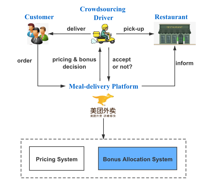
Figure 1. The typical process in the meal delivery platform.

need to add description

NA-canceled order is the main reason for negative ratings of the platform, taking Meituan as an example, about 30,000 negative reviews are received every day, and NA-canceled orders cause over 55% of them. Moreover, about 165,000 NA-canceled orders take place every day, which means less income for the crowdsourcing drivers, more food waste for restaurants, and a lower reputation of the meal delivery platform. The meal delivery platform needs to compensate the cost price of the restaurant’s food waste due to the platform’s responsibility, which is about billions of RMB for NA-canceled orders per year.

Through analyzing the historical data, the NA-canceled orders are led by following two main reasons: On one hand, the delivery price of some orders is not attractive enough to drivers, although the number of drivers is enough to satisfy the delivery demands. On the other hand, in some cases, the number of drivers can not enough to serve incoming orders, such as the lack of drivers online in the stormy weather. In this paper, we only focus on encouraging the driver to accept more orders in the first case. The second case, caused by extreme weather, is beyond the scope of this article.

Bonus allocation is a straightforward and effective way to encourage the drivers to accept the orders. In reality, an order is pushed to multiple nearby drivers simultaneously, and the acceptance probability of an order drops significantly with the time passing due to the potential risk of delay increasing. To motivate drivers to accept more orders and improve the efficiency of subsidy, the platform tends to allocate the bonus based on the empirical rule. For example, it allocates three RMB for the orders unaccepted within ten minutes, six RMB for twenty minutes, and so on. This method is easy to implement, it fails to achieve satisfactory performance since it offers a same price for all orders on every single decision stage separately and lacks global planning. The order’s life cycle could be split to multiple decision stages, and the order might be accepted, unaccepted, or canceled at each stage. If an order is not accepted by drivers or canceled by the consumer at a particular stage, it would be transited to the next stage. Once it is accepted by a driver or canceled by the consumer at a particular stage, its life cycle stops. If no drivers take the order for more than 50 minutes, the meal delivery platform will cancel it forcibly. Although most orders would be accepted in the first few stages, there still exist a considerable number of orders unaccepted until the last few stages. Intuitively, a better bonus allocation strategy should be globally optimized based on multi-stage information.

This paper develops a Multi-Stage Bonus Allocation (MSBA) framework for the bonus allocation problem on the meal delivery platform. Zhao et al.(Zhao et al., 2019) studied a marketing budget allocation problem similar to ours. However, they solved a single-stage problem while we dealt with a multi-stage one. To the best of our knowledge, this is the first study to discuss MSBA for the meal delivery platform, which is not trivial because of the following challenges:

• The bonus decided on each stage is just a display bonus, and will be paid to the driver only when the order is accepted. So this problem involves both multi-stage decision-making and complicated budget allocation.

• In reality, the bonus allocation decision for an order must be performed in milliseconds. An efficient algorithm is proposed to generate fast and efficient bonus allocation decisions to meet such a stringent computational target.

• The total amount of available bonuses is limited to a predetermined monthly budget, but all the orders placed within a month cannot be obtained beforehand. Therefore, solving this problem faces two challenges: 1. How to effectively use historical information to make current decisions. 2. How to dynamically adjust the strategy based on the randomly placed orders that have been generated in the current month.

The main contribution of this study is the development of an MSBA framework. This framework includes an acceptance and cancellation model, a Lagrangian dual-based dynamic programming (LDDP) algorithm, an online allocation algorithm, and a periodic control strategy. The acceptance model is employed to forecast the relationship between the bonus allocated to order and its acceptance probability. The cancellation probability is estimated for each order by an XGBoost (Chen et al., 2015) model at each stage. The LDDP algorithm, which is the backbone of the framework, is developed to calculate an effective parameter (Lagrangian multiplier (Yang and Huang, 2001)) for each allocation stage offline based on the historical dataset. The resulting Lagrangian multipliers are used to infer the bonus allocation decisions online. Finally, we use periodic control strategies to adapt the remained budget and order set dynamically so that the cost meets the total budget constraint. Efficiently, the proposed framework can make quick decisions in real-time with the computational complexity of O(1) for online calculation. Our online A/B tests show that compared with single-stage allocation method, the number of cancelled orders reduces more than 25%. Furthermore, we can save more than 30% of the compensation paid to restaurants for food waste. In addition, the proposed method could be also applied to similar time-series pricing problems, such as discounts on products near expiration date in supermarkets, price design of perishable products, etc. The proposed algorithm has been already actually applied in the largest meal delivery platform in China.

2. Problem Formulation

2.1. The Acceptance and Cancellation Model

As previously mentioned, MSBA aims to maximize the number of accepted orders. To formulate this, our objective function is to maximize the expected value of the number of accepted orders based on the acceptance probability of orders. With multiple allocation stages, an unaccepted and not canceled order from a former allocation stage is transited to the next allocation stage. The transition process of the order is illustrated in Figure 2. Each node represents an allocation stage. Let $p_{1}$ be the acceptance probability in the first allocation stage,$q_{1}$ be the cancellation probability in the first allocation stage. Correspondingly, $1-p_{1}-q_{1}$ is the probability of transitioning to the second allocation stage. Consequently, the probability that an order can enter $|T|$ stage is $\prod_{t_{0}=1}^{|T-1|}(1-p_{t_{0}}-q_{t_{0}})$. Otherwise, the order is accepted in $|T|$ stage with the probability of $\prod_{t_{0}=1}^{|T-1|}(1-p_{t_{0}}-q_{t_{0}})p_{|T|}$. In total, the probability of an order being accepted is expressed as follows:

(1) $$p=\sum_{t=1}^{|T|}\prod_{t_{0}=1}^{t-1}(1-p_{t_{0}}-q_{t_{0}})p_{|T|}$$

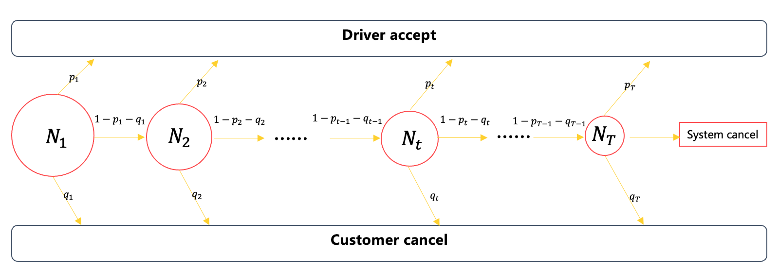
Figure 2. The transition process of an order.

need to add description

We need to forecast the relationship between the bonus allocated to orders and its acceptance probability to make optimal delivery bonus allocation decisions. To simplify the calculation, we assume that if the order is still on the waiting list, the probability of acceptance of the order at stage $t$ is only determined by the price of the order at stage $t$. The price of the order at other stages and the price of other orders do not affect the acceptance probability of this order.

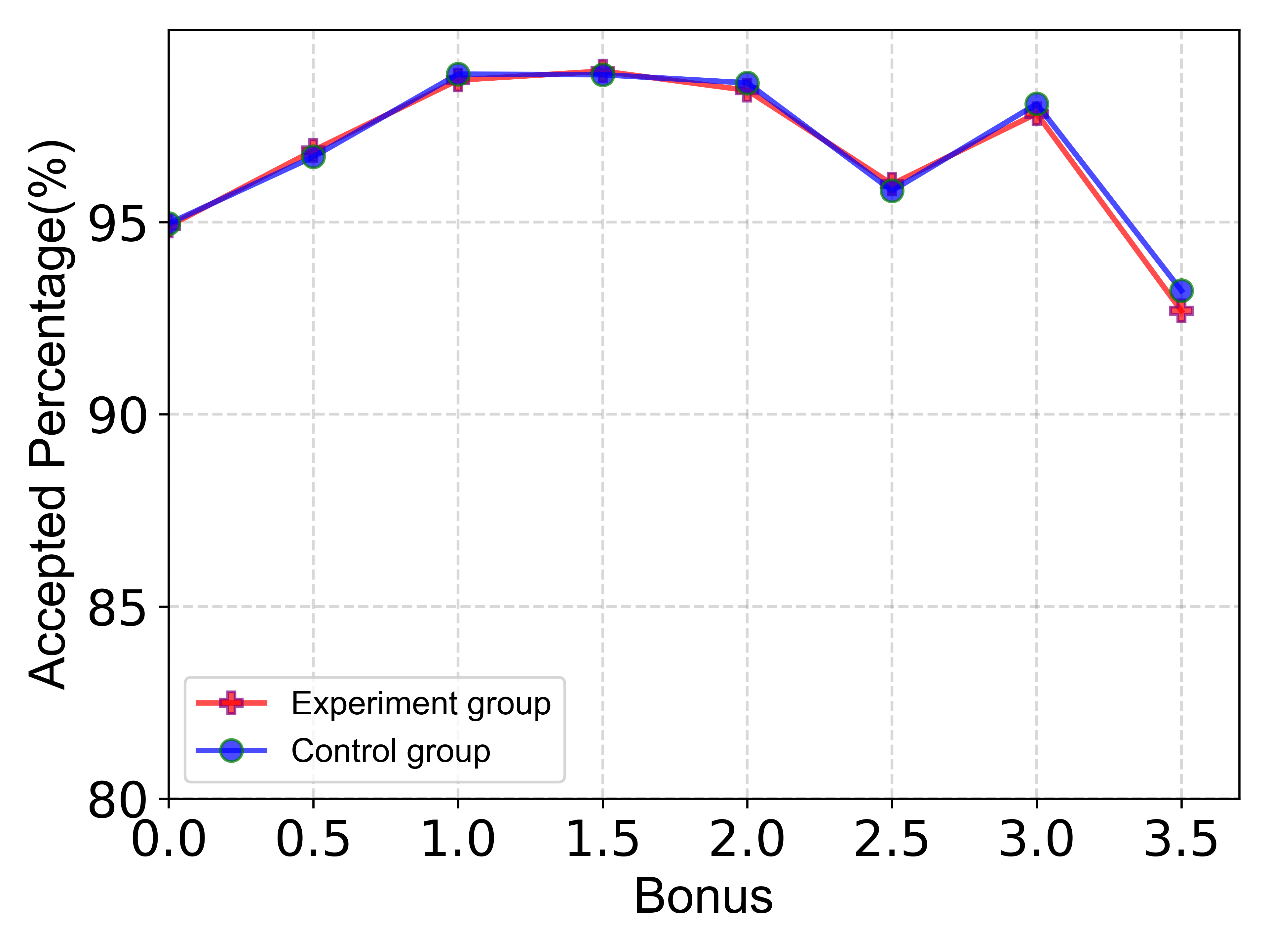
Figure 3. The proportion of orders accepted within 10 minutes.

need to add description

To test this hypothesis in real cases, we further conduct an ablation study. Orders are divided into the experiment group and the control group. We give a fixed bonus changing from 0.0 to 3.5 if the orders are not picked up within 10 minutes in the experiment group, while there is no bonus in the control group. Figure 3 shows the accepted rate of the orders within 10 minutes for different bonus level. It shows that the strategy of bonus after 10 minutes neither affects the drivers’ decisions within 10 minutes, nor causes the drivers to wait for bonus, thus the accepted rate of the two groups within 10 minutes is nearly the same. Hence, the hypothesis is to some extent valid in our real delivery system.

In this study, we adopt a semi-black-box forecasting model. We assume that the acceptance probability model conforms to the following logistic function:

(2) $$p_{i,t}(c_{i,t})=\frac{1}{1+e^{\alpha_{i,t}c_{i,t}+\beta_{i,t}}}$$

Meanwhile, $\alpha_{i,t}$ and $\beta_{i,t}$ are attained by the machine learning model such as a neural network. The input features of the forecasting model can be split into two different parts: the bonus allocated to each order $c_{i,t}$ and contextual features $\boldsymbol{x_{i,t}}$. Contextual features are intrinsic attributes of the order, including the geographical locations of the customer and the restaurant, the time difference between the current time and the user’s order, estimated time of arrival (ETA), the influence of the supply and demand related to drivers, the drivers’ spatial information (e.g. the number of drivers within 2 kilometers of the restaurant), and others. The contextual features contain information as much as available unless prohibited by local law.

The training set $\{[\boldsymbol{x_{i,t}},c_{i,t}],p_{i,t}^{*}\}$ is constructed for each order $i$ at each allocation stage $t$ from historical observations. Contrary to the method in the reference(Zhao et al., 2019) where $\alpha_{i,t}$ and $\beta_{i,t}$ are learned separately, in this study, we learn $\alpha_{i,t}$ and $\beta_{i,t}$ simultaneously but with different hidden layers (see Figure 4). In practice, the bonus is only allocated to a minority of orders such that the sample distribution of the training set is uneven. Therefore, we divide the training set into two kinds of batches: bonus batches with $c_{i,t}>0$ and normal batches with $c_{i,t}=0$. As in reference(Zhao et al., 2019), $\beta_{i,t}$ is determined by contextual features $\boldsymbol{x_{i,t}}$. Therefore, to improve the performance of the model, the hidden layers of $\alpha_{i,t}$ and $\beta_{i,t}$ are updated using different kinds of batches. More specifically, the bonus batches are used to update the parameters of hidden layer 0 and layer 1, and the normal batches are used to do the same for hidden layer 0 and layer 2. Note that the attained $\alpha_{i,t}$ should be less than 0, which is consistent with the common sense of the more the bonus, the larger the acceptance probability.

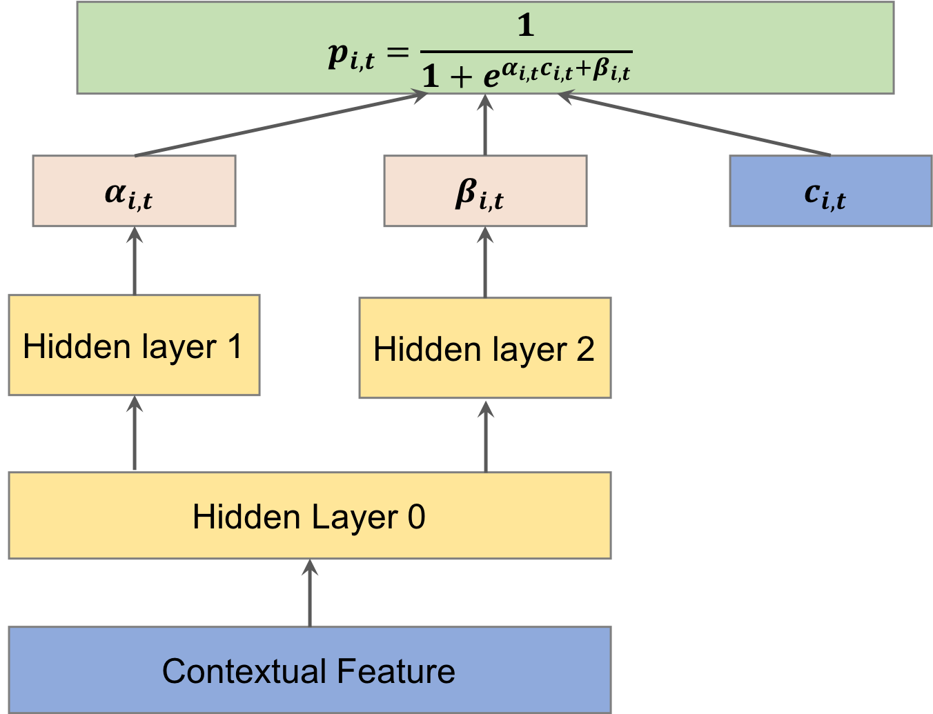
Figure 4. The illustration of the acceptance probability model.

need to add description

The acceptance probability model of orders is illustrated in Figure 5. As shown, the acceptance probabilities of the two orders may differ, even though their delivery bonus is the same. The acceptance probability (over 95%) is much higher than that of order B(approximately 45%) when the bonus is 0. Given the bonus of 2 RMB, the increment of acceptance probability of order A is 0.01, whereas order B is 0.38. Therefore, the motivation is to increase the total acceptance probability by allocating a bonus to order B.

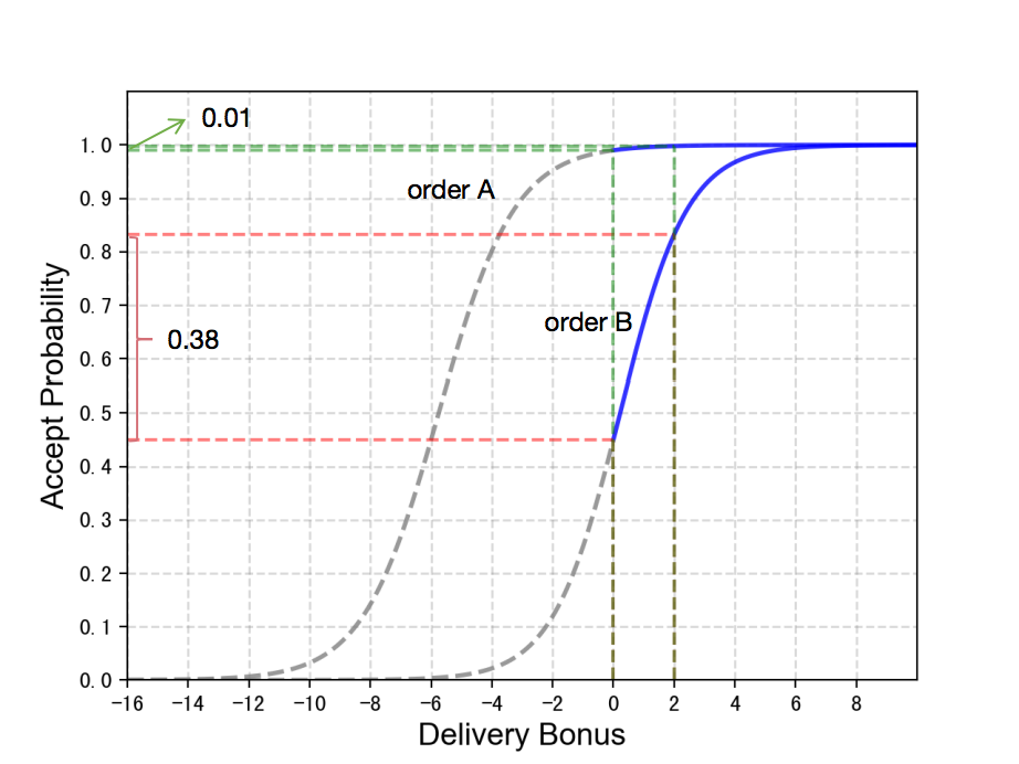
Figure 5. The relationship between the bonus and acceptance probability.

need to add description

The cancellation rate of order in $|T|$ stage also affects our decision, so we need to forecast it, which is marked as Symbol $q_{|T|}$. We have selected all orders entering the $|T|$ stage as a complete sample set. The characteristics of the sample are the relevant attributes of the order entering the stage, such as distance, environment, weather, and other characteristics. The label of the sample is that the canceled orders at this stage are marked as 1, and the other orders are marked as 0. We use the classic XGBoost model to train these samples to get the corresponding estimation model. Then we decompose the predicted value of the model at this stage. Each 0.05 forecast value interval is divided into one category, and each type of order is frequently sampled, and the proportion of positive samples within the interval is counted. This ratio is considered to be a predicted value which is the actual cancellation probability of the order in the region.

2.2. Definition and Mathematical Model

The set $N$ consists of the order placed within a week/month.The set $T$ means the bonus allocation stage set, i.e., the bonus allocated to an order can be changed at most $|T|$ times.Let $p_{i,t}$ be the acceptance probability of the order $i$ at allocation stage $t\in T$,$q_{i,t}$ be the cancellation probability of the order $i$ at allocation stage $t\in T$. The decision variable $c_{i,t}$ is the delivery bonus of the order $i\in N$ at allocation stage $t\in T$. The upper bound of the delivery bonus is $C_{i}^{u}$ . The function $p_{i,t}(c_{i,t})$ denotes the acceptance probability model of the order $i\in N$ if it is transited to allocation stage $t\in T$. The total delivery bonus cost should be within the given budget $B$. The MSBA is modeled as follows:

(3) $$\max~{} \sum_{i\in N}\sum_{t\in T}(\prod_{t_{0}=1}^{t-1}(1-p_{i,t_{0}}(c_{i,t_{0}})-q_{i,t_{0}}))p_{i,t}(c_{i,t})$$

(4) s.t. $$\sum_{i\in N}\sum_{t\in T}(\prod_{t_{0}=1}^{t-1}(1-p_{i,t_{0}}(c_{i,t_{0}})-q_{i,t_{0}}))p_{i,t}(c_{i,t})c_{i,t}\leq B$$

(5) $$0\leq c_{i,t}\leq C_{i}^{u}\qquad\forall i\in N,t\in T$$

The objective function (3) maximizes the total acceptance probability, i.e., the excepted value of the accepted order quantity. Constraint (4) indicates that the expected value of the total delivery bonus cost should be within the given budget B. Constraints (5) restrain the delivery bonus $c_{i,t}$ within the given upper bound.

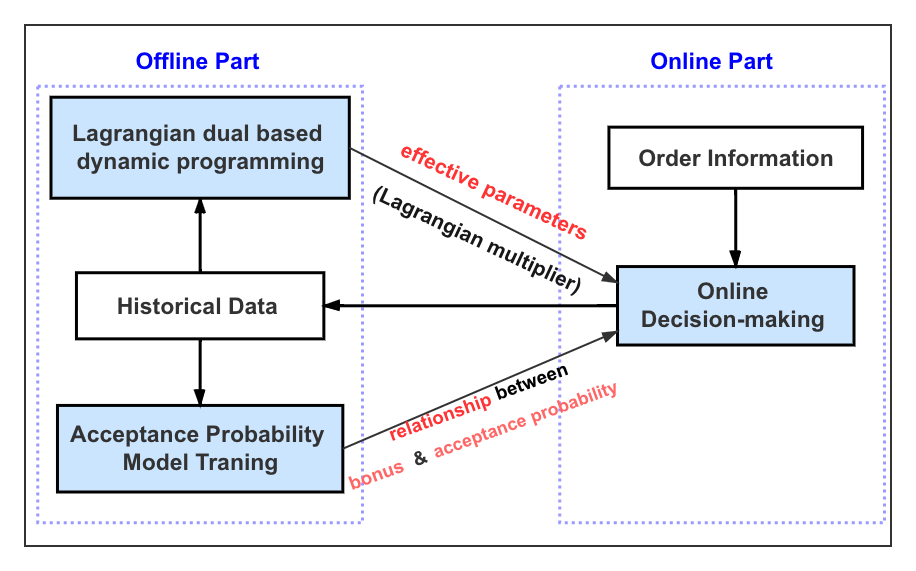
Figure 6. Our multi-stage bonus allocation framework.

need to add description

3. Algorithm

The framework of our bonus allocation approach is shown in Fig. 6. Our algorithm contains an offline part, the Lagrangian Dual-based Dynamic Programming (LDDP), to solve Problem (3) based on the historical dataset, and an online part to satisfy fast real-time calculation of budget allocation. The offline part first optimizes Problem (3) and calculates the empirical Lagrangian multiplier $\lambda^{*}_{t}$ for each allocation stage $t$, and the online part uses the optimal $\lambda^{*}_{t}$ to make real-time bonus allocation decisions online.

3.1. Offline Optimization: The Lagrangian Dual-based Dynamic Programming

Problem (3) is a non-linear and non-convex multi-stage optimization problem, which is intractable in practice. In this section, we propose a novel LDDP method to solve this problem. We view this problem as a combination of two sub-problems. First, we allocate the total budget to each stage, and then within each stage, we calculate the optimal bonus for each order. The former sub-problem could be dealt with dynamic programming, and the latter one is a standard single-stage allocation problem solved by Lagrangian dual theory.

Let $N_{\tilde{t}}$ be the remaining order set transited to allocation stage $\tilde{t}$, if there is no budget posed on stage 1 to $\tilde{t}-1$. Thinking of the right-hand side of constraint (4) $\tilde{B}$ taking value $0,1,2,\cdots,B$ as money level. Note that we discretize the budget to decrease the complexity of the algorithm and meet real-world conditions. The allocation stage subset $\{\tilde{t},\tilde{t}+1,...,|T|\}$ represented by $\tilde{t}$ as the ”stage”(Note that this ”stage” is used to define a sub-problem of dynamic programming, which is different from the allocation stage mentioned before), leads us to define the subproblem $P_{\tilde{t}}(\tilde{B})$ and the optimal value function $G_{\tilde{t}}(\tilde{B})$ as follows:

(6) $$G_{\tilde{t}}(\tilde{B})=\max~{} \sum_{i\in N_{\tilde{t}}}\sum_{t=\tilde{t}}^{|T|}(\prod_{t_{0}=\tilde{t}}^{t-1}(1-p_{i,t_{0}}(c_{i,t_{0}})-q_{i,t_{0}}))p_{i,t}(c_{i,t})$$

(7) s.t. $$\sum_{i\in N_{\tilde{t}}}\sum_{t=\tilde{t}}^{|T|}(\prod_{t_{0}=\tilde{t}}^{t-1}(1-p_{i,t_{0}}(c_{i,t_{0}})-q_{i,t_{0}}))p_{i,t}(c_{i,t})c_{i,t}\leq\tilde{B}$$

(8) $$0\leq c_{i,t}\leq C_{i}^{u},\forall i\in N_{\tilde{t}},t=\tilde{t},\tilde{t}+1,...,|T|$$

Then, $z=G_{1}(B)$ gives us the optimal value of the MSBA(Wolsey, 1998).

To define a recursion that allows us to calculate $G_{\tilde{t}}(\tilde{B})$ in terms of $G_{s}(\tilde{B_{0}})$ for $s>\tilde{t}$ and $\tilde{B_{0}}\leq\tilde{B}$, we need to define a single-stage bonus allocation problem with the objective value function $g_{\tilde{t}}(\tilde{B})$, where budget $\tilde{B}$ is only spent on a single stage $\tilde{t}$. It indicates the optimal expected value of the accepted order quantity if budget $\tilde{B}$ is spent on a single stage $\tilde{t}$. Function $g_{\tilde{t}}(\tilde{B})$ is expressed as follows:

(9) $$g_{\tilde{t}}(\tilde{B})=\max~{} \sum_{i\in N_{\tilde{t}}}p_{i,\tilde{t}}(c_{i,\tilde{t}})$$

(10) s.t. $$\sum_{i\in N_{\tilde{t}}}p_{i,\tilde{t}}(c_{i,\tilde{t}})c_{i,\tilde{t}}\leq\tilde{B}$$

(11) $$0\leq c_{i,\tilde{t}}\leq C_{i}^{u} \forall i\in N_{\tilde{t}}$$

By solving the single-stage bonus allocation problem with single-stage budget $\tilde{B}=k$, we can attain the accepted probability vector. $\boldsymbol{p}_{\tilde{t}}(k)=[p_{1,\tilde{t}}(c_{1,\tilde{t}}(k)),p_{2,\tilde{t}}(c_{2,\tilde{t}}(k)),...,p_{|N_{\tilde{t}}|,\tilde{t}}(c_{|N_{\tilde{t}}|,\tilde{t}}(k))]$, where $c_{i,\tilde{t}}(k)$ is the optimal bonus for order $i$ under total budget $k$ constraint on stage $\tilde{t}$.

Then, $G_{\tilde{t}}(\tilde{B})$ can be expressed as follows:

(12) $$G_{\tilde{t}}(\tilde{B})=\max_{k=0,1,...,\tilde{B}}\{g_{\tilde{t}}(k)+G^{\prime}_{\tilde{t}+1}(\tilde{B}-k)\}$$

$G^{\prime}_{\tilde{t}+1}(\tilde{B}-k)$ indicates the optimal value function with budget of $\tilde{B}-k$ spent on allocation stage set $\{\tilde{t}+1,...,|T|\}$, under the condition that budget of $k$ is spent on single allocation stage $\tilde{t}$. $G^{\prime}_{\tilde{t}+1}(\tilde{B}-k)$ can be formulated as follows (Let $x_{i}$ be $\sum_{t=\tilde{t}+1}^{|T|}(\prod_{t_{0}=\tilde{t}}^{t-1}(1-p_{i,t_{0}}(c_{i,t_{0}})-q_{i,t_{0}}))p_{i,t}(c_{i,t})$ in the following expressions for short.):

(13) $$G^{\prime}_{\tilde{t}+1}(\tilde{B}-k)=\max~{} \sum_{i\in N_{\tilde{t}}}(1-p_{i,\tilde{t}}(k)-q_{i,\tilde{t}})x_{i}$$

(14) s.t. $$\sum_{i\in N_{\tilde{t}}}(1-p_{i,\tilde{t}}(k)-q_{i,\tilde{t}})x_{i}c_{i,t}\leq\tilde{B}-k$$

(15) $$0\leq c_{i,t}\leq C_{i}^{u},\forall i\in N_{\tilde{t}},t=\tilde{t}+1,...,|T|$$

3.1.1. Dimensionality Reduction

Noticing that the definition of $G$ and $G^{\prime}$ in (12) is different, which is hard for dynamic programming. Hence, we must establish link between two optimization problems.

The main difference for $G_{\tilde{t}+1}(\tilde{B})$ and $G^{\prime}_{\tilde{t}+1}(\tilde{B})$ is that $G_{\tilde{t}+1}(\tilde{B})$ is calculated by $\boldsymbol{1}^{T}\boldsymbol{x}$, while $G^{\prime}_{\tilde{t}+1}(\tilde{B})$ is calculated by $(\boldsymbol{1}-\boldsymbol{p}_{\tilde{t}}(k)-\boldsymbol{q}_{\tilde{t}})^{T}\boldsymbol{x}$, in both objective function and constraint. A simple way to reduce complexity is to project vector $\boldsymbol{p}_{\tilde{t}}(k)+\boldsymbol{q}_{\tilde{t}}$ to an m-dimensional space under a predefined projection matrix, i.e. $\boldsymbol{p}_{\tilde{t}}(k)+\boldsymbol{q}_{\tilde{t}}\approx\boldsymbol{H}\boldsymbol{u}$, where $\boldsymbol{H}$ is a predefined $(|N_{\tilde{t}}|\times m)$-dimensional projection matrix. Under such decomposition (Birge, 1985), the objective function of $G^{\prime}_{\tilde{t}+1}(\tilde{B})$ could be written as a form of $\boldsymbol{1}^{T}\boldsymbol{x}-\boldsymbol{u}^{T}\boldsymbol{H}^{T}\boldsymbol{x}$.

To satisfy the computational requirement of industry in practice, we reduce the number of dimension $m$ to 1 in our work. In this simplest way, we choose $\boldsymbol{H}$ as $[1,1,\cdots,1]$ and hence $u=\frac{\sum_{N_{\tilde{t}}}(p_{i,\tilde{t}}(k)+q_{\tilde{t}})}{|N_{\tilde{t}}|}$ representing for the average probability for orders accepted or cancelled on stage $\tilde{t}$. We immediately build up the relationship between $G^{\prime}_{\tilde{t}+1}(\tilde{B})$ and $G_{\tilde{t}+1}(\tilde{B})$: (1) the equivalence of the objective function: $\boldsymbol{1}^{T}\boldsymbol{x}-u\boldsymbol{H}^{T}\boldsymbol{x}=(1-u)\boldsymbol{1}^{T}\boldsymbol{x}$. (2) the equivalence of the constraint:

(16) $$\sum_{i\in N_{\tilde{t}}}(1-p_{i,\tilde{t}}(k)-q_{i,\tilde{t}})x_{i}c_{i,t}\leq\tilde{B}\iff\sum_{i\in N_{\tilde{t}}}x_{i}c_{i,t}\leq\frac{\tilde{B}}{1-u}$$

In other words, there must be $G^{\prime}_{\tilde{t}+1}(\tilde{B})=(1-u)G_{\tilde{t}+1}(\frac{\tilde{B}}{1-u})$. By dimensionality reduction, we sacrifice a little accuracy in change of low time complexity for dynamic programming (Si et al., 2004).

3.1.2. Recursion to Dynamic Programming

Formally, as $\sum_{i\in N_{\tilde{t}}}p_{i,\tilde{t}}(k)=g_{t}(k)$ holds according to the definition of $\boldsymbol{p}_{\tilde{t}}(k)$. Moreover, we define $\sum_{i\in N_{\tilde{t}}}q_{i,\tilde{t}}=Q_{t}$. Therefore, $G^{\prime}_{\tilde{t}+1}(\tilde{B}-k)$ is formulated as follows:

(17) $$G^{\prime}_{\tilde{t}+1}(\tilde{B}-k)=\max~{} \frac{|N_{\tilde{t}}|-g_{t}(k)-Q_{t}}{|N_{\tilde{t}}|}\sum_{i\in N_{\tilde{t}}}x_{i}$$

(18) s.t. $$\sum_{i\in N_{\tilde{t}}}x_{i}c_{i,t}\leq\frac{|N_{\tilde{t}}|}{|N_{\tilde{t}}|-g_{t}(k)-Q_{t}}\tilde{B}-k$$

(19) $$0\leq c_{i,t}\leq C_{i}^{u},\forall i\in N_{\tilde{t}},t=\tilde{t}+1,...,|T|$$

In summary, the expression (12) can be reformulated as the recursion as follows:

(20) $$G_{\tilde{t}}(\tilde{B})=\max_{k=0,1,...,\tilde{B}}\{g_{\tilde{t}}(k)+\frac{|N_{\tilde{t}+1}|}{|N_{\tilde{t}}|}*G_{\tilde{t}+1}[(\tilde{B}-k)\frac{|N_{\tilde{t}}|}{|N_{\tilde{t}+1}|}]\}$$

where $|N_{\tilde{t}+1}|=|N_{\tilde{t}}|-g_{t}(k)-Q_{t}$. Starting the recursion with $G_{|T|}(\tilde{B})=g_{|T|}(\tilde{B})$ for $\tilde{B}\geq 0$, we use the recursion (20) to successively calculate $G_{|T|-1},G_{|T|-2},...,G_{1}$ for all integral values of $\tilde{B}$ from 0 to B. An overview of the dynamic programming algorithm is presented in Algorithm 1. In this process, we must solve a single-stage bonus allocation problem with objective value of $g_{\tilde{t}}(\tilde{B})$ for all $\tilde{t}\in T$ and $\tilde{B}\in\{0,1,2,...,B\}$.

Input: Allocation stage set $T$, order set $N_{\tilde{t}},\forall t\in T$, total budget B

Output: empirical Lagrangian Multipliers $\lambda^{*}[|T|]$

 $\triangleright$ Solve the single-stage bonus allocation repeatedly and obtain $g[|T|][B]$ and $\lambda[|T|][B]$

1 forall $\tilde{t}\in T$ do

2       while $\tilde{B}$¡=B do

3             $g[\tilde{t}][\tilde{B}],\lambda[\tilde{t}][\tilde{B}]\leftarrow BA(N_{\tilde{t}},\tilde{B})$

4             $\tilde{B}\leftarrow\tilde{B}+1$

5            

6      

 $\triangleright$ Solve the sub-problem $P_{\tilde{t}}(\tilde{B})$ recursively and obtain G[|T|][B], then estimate the probability of order cancellation at stage ${\tilde{t}}$ and sum it up,get the corresponding $Q[\tilde{t}]$

7 $G[|T|]\leftarrow g[|T|]$

8 $\tilde{t}\leftarrow|T|-1$

9 $\tilde{B}\leftarrow 0$

10 while $\tilde{t}\geq 1$ do

11       while $\tilde{B}$¡=B do

12             $G[\tilde{t}][\tilde{B}]\leftarrow G[\tilde{t}+1][\tilde{B}]$

13             $k^{*}\leftarrow 0$

14             for $k\leftarrow 0$ to $\tilde{B}$ by $1$ do

15                   $N^{\prime}\leftarrow|N_{\tilde{t}}|-g[\tilde{t}][k]-Q[\tilde{t}]$

16                   $temp\leftarrow g[\tilde{t}][k]+\frac{N^{\prime}}{|N_{\tilde{t}}|}G[\tilde{t}+1][\lfloor{\frac{|N_{\tilde{t}}|}{N^{\prime}}(\tilde{B}-k)}\rfloor]$

17                   if $G[\tilde{t}][\tilde{B}]<temp$ then

18                        $G[\tilde{t}][\tilde{B}]\leftarrow temp$

19                         $k^{*}\leftarrow k$

20                        

21                  

            $a[\tilde{t}][\tilde{B}]\leftarrow k^{*}$

             $\triangleright$ a[][] is used to backtrack the optimal Lagrangian multiplier for each allocation stage

22             $\tilde{B}\leftarrow\tilde{B}+1$

23            

24      $\tilde{t}\leftarrow\tilde{t}-1$

 $\triangleright$ Backtrack the optimal solution and record the optimal empirical Lagrangian multiplier for each stage into arrays $\lambda^{*}[|T|]$

25 $B_{0}\leftarrow B$

26 for $t=1$ to $|T|$ by $1$ do

27       $B^{*}\leftarrow a[t][B_{0}]$

28       $\lambda^{*}[t]\leftarrow\lambda[t][B^{*}]$

29       $B_{0}\leftarrow B_{0}-B^{*}$

return $\lambda^{*}[|T|]$

Algorithm 1 Lagrangian dual-based Dynamic Programming

3.1.3. Solve Single-stage Bonus Allocation Problem Based on Lagrangian Dual Theory

As defined by functions (9)-(11), both the objective function and constraint functions are non-convex with respect to $\boldsymbol{c}$. Therefore, solving the problem directly is very difficult. Inspired by (Zhao et al., 2019; Dong et al., 2009; Li and Huh, 2011), we reformulate the problem into an equivalent convex optimization problem. Because $p_{i,t}(c_{i,t})=\frac{1}{1+e^{\alpha_{i,t}c_{i,t}+\beta_{i,t}}}$, we have

(21) $$\begin{split}&c_{i,t}(p_{i,t})=-\frac{\beta_{i,t}}{\alpha_{i,t}}+\frac{1}{\alpha_{i,t}}(\ln(1-p_{i,t})-\ln(p_{i,t}))\\ &p_{i,t}\in(0,1),\forall i\in N,t\in T\end{split}$$

Consequently, the constraint function (10) is rewritten as a function of $p_{i,\tilde{t}}$:

(22) $$f_{\tilde{t}}(\boldsymbol{p})=\sum_{i\in N_{\tilde{t}}}p_{i,\tilde{t}}c_{i,\tilde{t}}(p_{i,\tilde{t}})\\$$

Referring to (Zhao et al., 2019; Dong et al., 2009; Li and Huh, 2011), $f_{\tilde{t}}(\boldsymbol{p})$ is a convex function in $\boldsymbol{p}$ for $\forall\tilde{t}\in T$.

Therefore, the original problem (9)-(11) is reformulated as follows:

(23) $$-g_{\tilde{t}}(\tilde{B})=\min~{} -\sum_{i\in N_{\tilde{t}}}p_{i,\tilde{t}}$$

(24) s.t. $$\sum_{i\in N_{\tilde{t}}}p_{i,\tilde{t}}c_{i,\tilde{t}}(p_{i,\tilde{t}})\leq\tilde{B}$$

(25) $$P_{i}^{l}\leq p_{i,\tilde{t}}\leq P_{i}^{u} \forall i\in N_{\tilde{t}}$$

Clearly, this is a differentiable convex optimization problem with respect to $\boldsymbol{p}$ and Slater’s condition holds easily. The duality gap between the primal and dual objective value equals to 0(Boyd et al., 2004).

By introducing a dual variable $\lambda$, the Lagrangian relaxation function of the single-stage bonus allocation problem is represented as follows:

(26) $$L(\boldsymbol{p},\lambda)=~{}-\sum_{i\in N_{\tilde{t}}}p_{i,\tilde{t}}+\lambda[\sum_{i\in N_{\tilde{t}}}p_{i,\tilde{t}}c_{i,\tilde{t}}(p_{i,\tilde{t}})-\tilde{B}]$$

where $P_{i}^{l}\leq p_{i,\tilde{t}}\leq P_{i}^{u}$,$\forall i\in N,\lambda\in\mathbb{R}_{+}$. Correspondingly, the Lagrangian dual problem is formulated as:

(27) $$\max_{\lambda\in\mathbb{R}_{+}}\min_{P_{i}^{l}\leq p_{i,\tilde{t}}\leq P_{i}^{u}}L(\boldsymbol{p},\lambda)$$

As mentioned before, the primal optimal value $-g_{\tilde{t}}(\tilde{B})$ is equal to the dual optimal value owing to the zero duality gap. By introducing a bisection algorithm represented in Algorithm 2, we can obtain the optimal solution $\lambda_{\tilde{t}}(\tilde{B})$ and the optimal value $g_{\tilde{t}}(\tilde{B})$.

Input: Order set $N_{\tilde{t}}$, budget $\tilde{B}$

Output: $\lambda_{t}(\tilde{B})$ and $g_{\tilde{t}}(\tilde{B})$

1 $low\leftarrow 0$

$high\leftarrow M$

 $\triangleright$ M is a big number

2 while $high-low>\epsilon$ do

3       $s\leftarrow 0$

4       $opt\leftarrow 0$

5       $mid\leftarrow\frac{high+low}{2}$

6       forall $i\in N_{\tilde{t}}$ do

7             $p_{i,\tilde{t}}^{*}\leftarrow\arg\min_{P_{i}^{l}\leq p_{i,\tilde{t}}\leq P_{i}^{u}}-p_{i,\tilde{t}}+mid*p_{i,\tilde{t}}c_{i,\tilde{t}}(p_{i,\tilde{t}})$

8             $s\leftarrow s+p_{i,\tilde{t}}^{*}c_{i,\tilde{t}}(p_{i,\tilde{t}}^{*})$

9             $opt\leftarrow opt-p_{i,\tilde{t}}^{*}$

10            

11      if $s-\tilde{B}\geq 0$ then

12            $low\leftarrow mid$

13      else

14            $high\leftarrow mid$

15      

return $\lambda_{t}(\tilde{B})\leftarrow high$, $g_{\tilde{t}}(\tilde{B})\leftarrow-opt$

Algorithm 2 Bisection Algorithm for a single-stage problem(BA($N_{\tilde{t}}$,$\tilde{B}$))

3.2. Online Allocation Algorithm

Given the multiplier $\lambda^{*}_{\tilde{t}}$ attained by the LDDP algorithm for stage $\tilde{t}\in T$, the online problem is written as:

(28) $$\min_{0\leq c_{i,\tilde{t}}\leq C_{i}^{u}}~{}\{-\sum_{i\in N_{\tilde{t}}}p_{i,\tilde{t}}(c_{i,\tilde{t}})+\lambda^{*}_{\tilde{t}}[\sum_{i\in N_{\tilde{t}}}p_{i,\tilde{t}}(c_{i,\tilde{t}})c_{i,\tilde{t}}]\}$$

which is equivalent to:

(29) $$\min_{0\leq c_{i,\tilde{t}}\leq C_{i}^{u}}~{}\{\sum_{i\in N_{\tilde{t}}}(\lambda^{*}_{\tilde{t}}p_{i,\tilde{t}}(c_{i,\tilde{t}})c_{i,\tilde{t}}-p_{i,\tilde{t}}(c_{i,\tilde{t}}))\}$$

The above problem is reformulated as the summation of —$N_{\tilde{t}}$— separable minimizing problems as follows:

(30) $$\sum_{i\in N_{\tilde{t}}}\min_{0\leq c_{i,\tilde{t}}\leq C_{i}^{u}}\{(\lambda^{*}_{\tilde{t}}p_{i,\tilde{t}}(c_{i,\tilde{t}})c_{i,\tilde{t}}-p_{i,\tilde{t}}(c_{i,\tilde{t}}))\}$$

Therefore, to determine the delivery bonus for a specific order, only a one-dimensional problem needs to be solved. An optimal solution for each separated problem can easily be obtained online. The optimal delivery bonus of a specific order $i\in N$ is expressed as follows:

(31) $$c^{*}_{i,\tilde{t}} =\arg\min_{0\leq c_{i,\tilde{t}}\leq C_{i}^{u}}\lambda^{*}_{\tilde{t}}p_{i,\tilde{t}}(c_{i,\tilde{t}})c_{i,\tilde{t}}-p_{i,\tilde{t}}(c_{i,\tilde{t}})$$

Because the bonus of the order $i$ ranges from 0 to $C_{i}^{u}$, and the number of potential bonuses is limited, the optimization problem (31) is easily solved by enumerating the potential bonus. Other numerical optimization methods are applicable, but we are not going to investigate them further here. Note that multiple problems can be solved in parallel here because the first problem is separated into multiple independent problems. The bonus decision for each order can be traversed to obtain the optimal solution. The complexity of determining the delivery bonus of an order online is O(1).

3.3. Periodic Control

At the beginning of the month, the total budget is worked out by business analysts, but the actual future monthly order size and distribution are unknown. Fortunately, history data shows that the monthly order distribution of the meal delivery platform is relatively stable and the deviation between offline historical orders and online orders is slight. To further satisfy the budget constraint under uncertain online scenario, we adopt some simple but effective periodic control strategies.

The first strategy is that we execute the offline decision-making system once a day, and the selected training set is the order data of the previous month from the current day. The target budget for offline training is calculated by the remaining budget of this month divided by the expected future order numbers of this month and multiply the total order numbers in the past 30 days. The second strategy is to adopt some simple control methods on realtime expenditure  (Hao et al., 2015). For example, when the proportion of total realtime expenditure to total budget is greater than 110%, we will reduce the bonus to some proportion ratio. When the proportion is less than 90%, we will increase the bonus. The ratio of upward and downward adjustment is positively correlated with the difference between the total realtime expenditure and total budget. These two strategies ensure that the online realtime expenditure could be controlled around the pre-defined budget within an acceptable range.

4. Experiments

To verify the effectiveness of this method, we present the results of both offline experiments and online A/B tests.

4.1. Performance of offline experiments

In this section, we conducted several offline experiments. The instances are generated on real-world data derived from the Meituan meal delivery platform. Without the loss of generality, we chose the instances of four cities named Lanzhou, Nanchang, Weihai, and Chengdu with different typical order sizes over one week. Specifically, the data sets contain 46,978, 71,427, 120,017, and 258,612 orders, respectively. The delivery bonus of each order is calculated within the upper bound, which the business manager sets. It is worth mentioning that the budget in the figures below indicates the average budget for each order, which makes the results comparable among instances with different numbers of orders. A typical order life cycle starts from the order placed time to order delivered time or order canceled time, and the number of allocation stages indicates the dynamic bonus allocation frequency. For example, if the order life cycle is 50 minutes and the number of allocation stages is 10, the bonus allocation decision is determined every 5 minutes.

4.1.1. Performance of the MSBA

In this section, we examine the performance of the MSBA method considering eight allocation stages and about a six-minute time interval between two allocation stages. A comparison of the results with the unified bonus mechanism in which the same delivery bonus is allocated to each order, single-stage bonus allocation(Zhao et al., 2019) and MSBA is presented in Figure 8(a). As shown in the figure, compared to the cases without bonus allocation, using an MSBA reduces the number of canceled orders by more than 60%. Moreover, it also shows that the MSBA outperforms the other two approaches. More specifically, compared to multi-stage bonus allocation and the single-stage bonus allocation, the number of canceled orders derived from the MSBA is around 20% and 40% lower, respectively. More importantly, for the instances with a more significant number of orders, the MSBA performs better, whereas the unified bonus mechanism and single-stage bonus allocation perform worse.

Figure 7 illustrates the total bonus allocation for each allocation stage for different methods. We observe that the total bonus allocation increases at first and then decreases as the allocation stage extends. To determine the potential reasons, we investigate the distribution of the accepted order numbers on these allocation stages. As shown in Figure 8(b), most orders are accepted immediately at the first allocation stage, and the number of accepted orders decreases as the allocation stage extends. Recall from Section 2.1 that our motivation was to increase the total acceptance probabilities of all orders by allocating delivery bonus to ”order B” instead of ”order A” (Figure 5). Correspondingly, orders with high acceptance probability play the role of ”order A”. Consequently, the total bonus allocated to the first stage is small because most ”order A” instances are accepted at the first stage, and the total allocated bonus increases at the early stages because of the number of ”order B” increases. Then, as the allocation stage extends, the total bonus decreases since the remaining orders decrease.

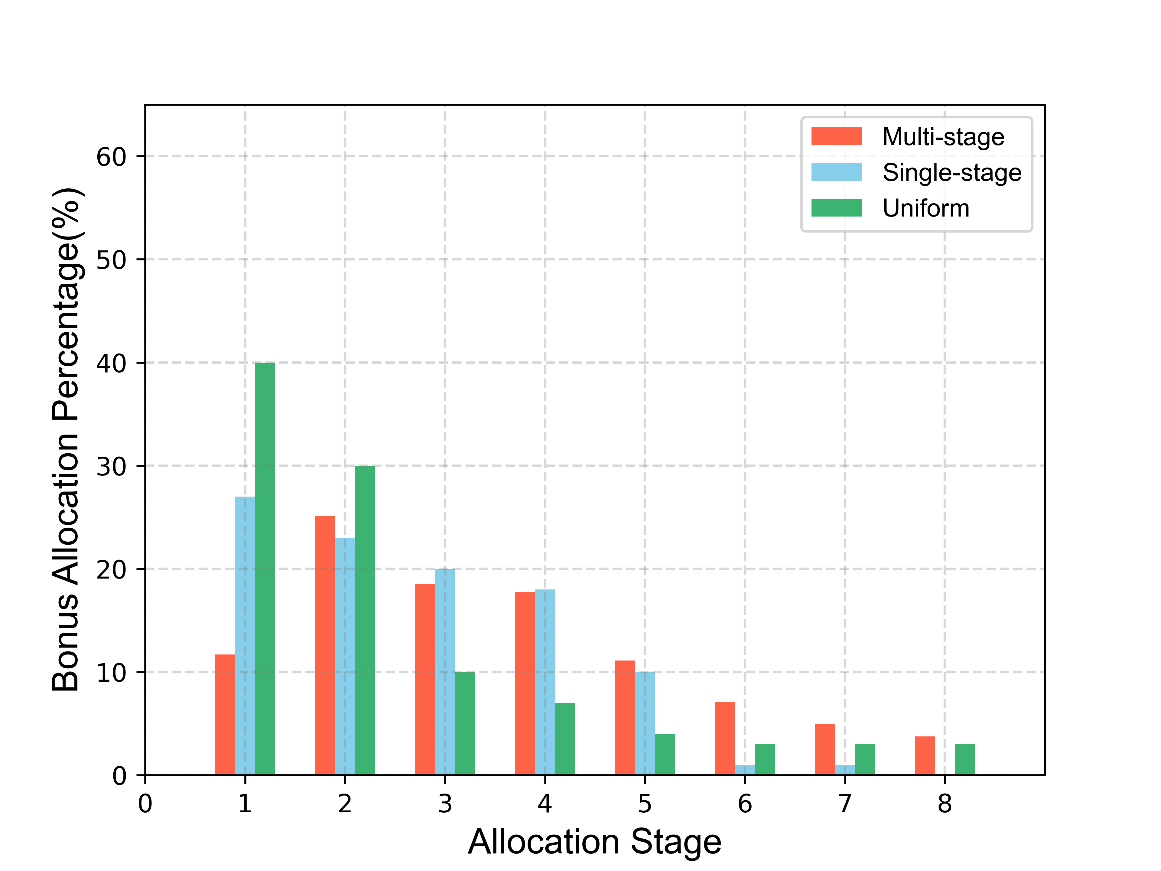
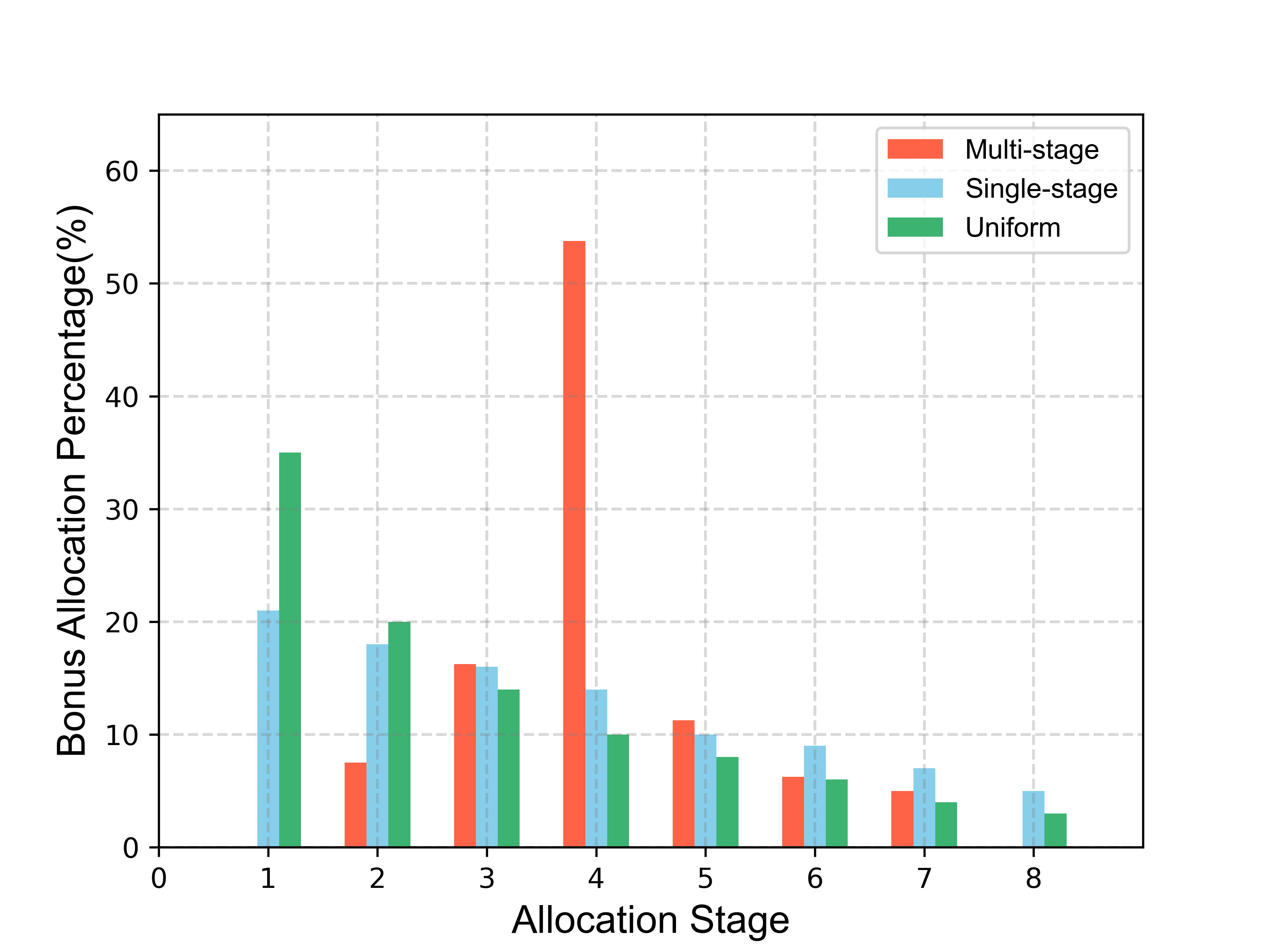
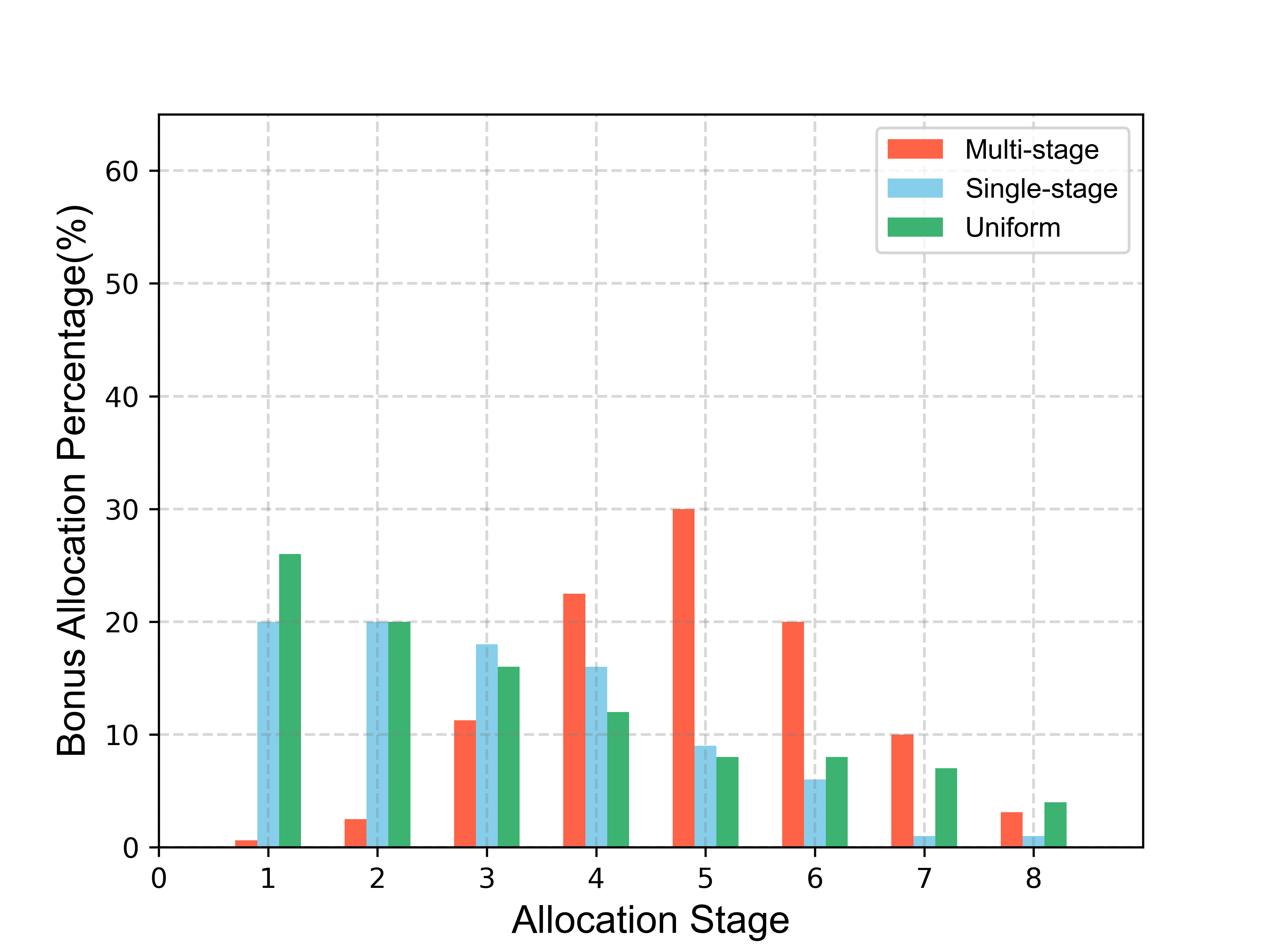
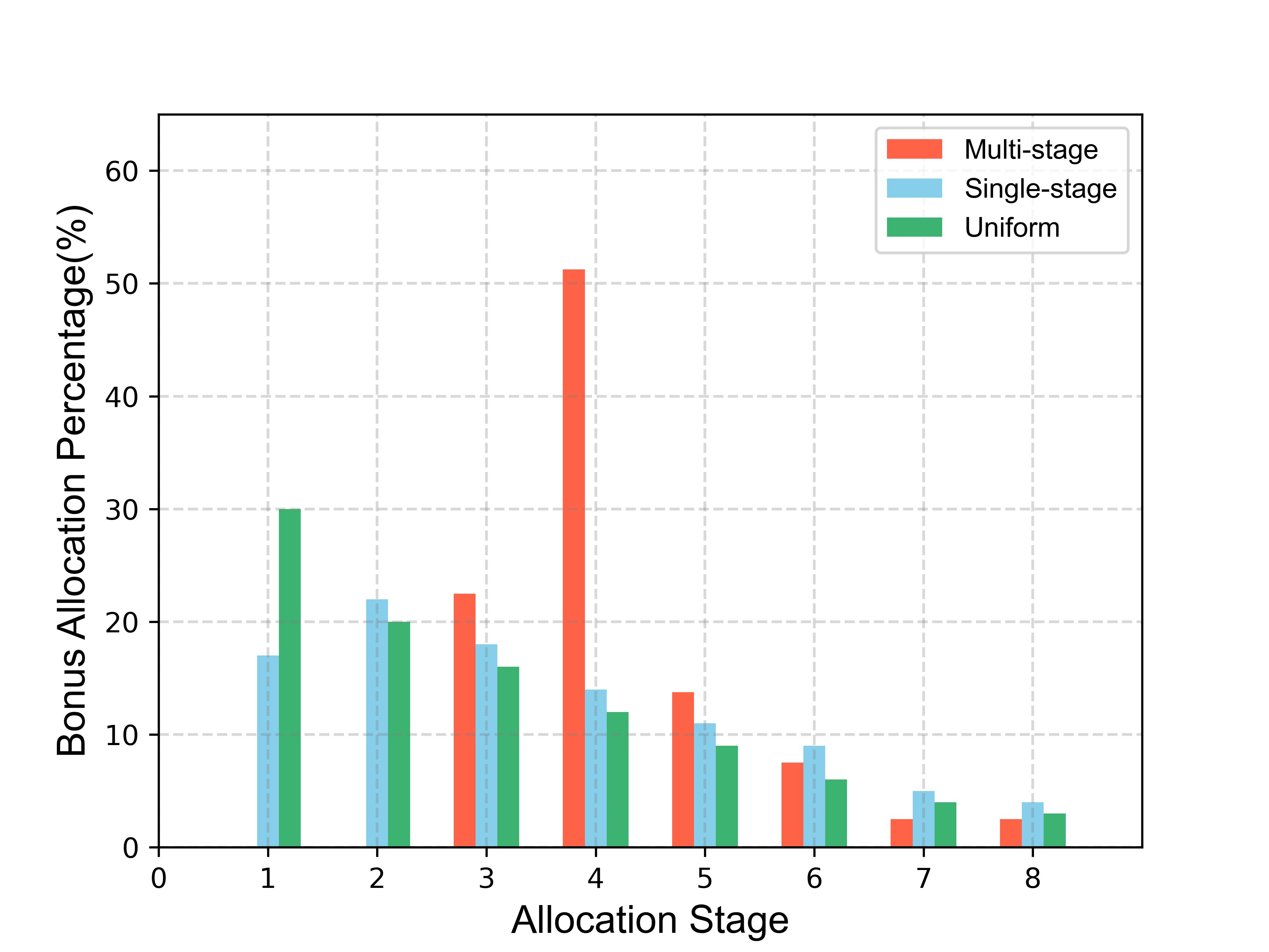
Figure 7. Total bonus allocation among all allocation stages with different approaches.

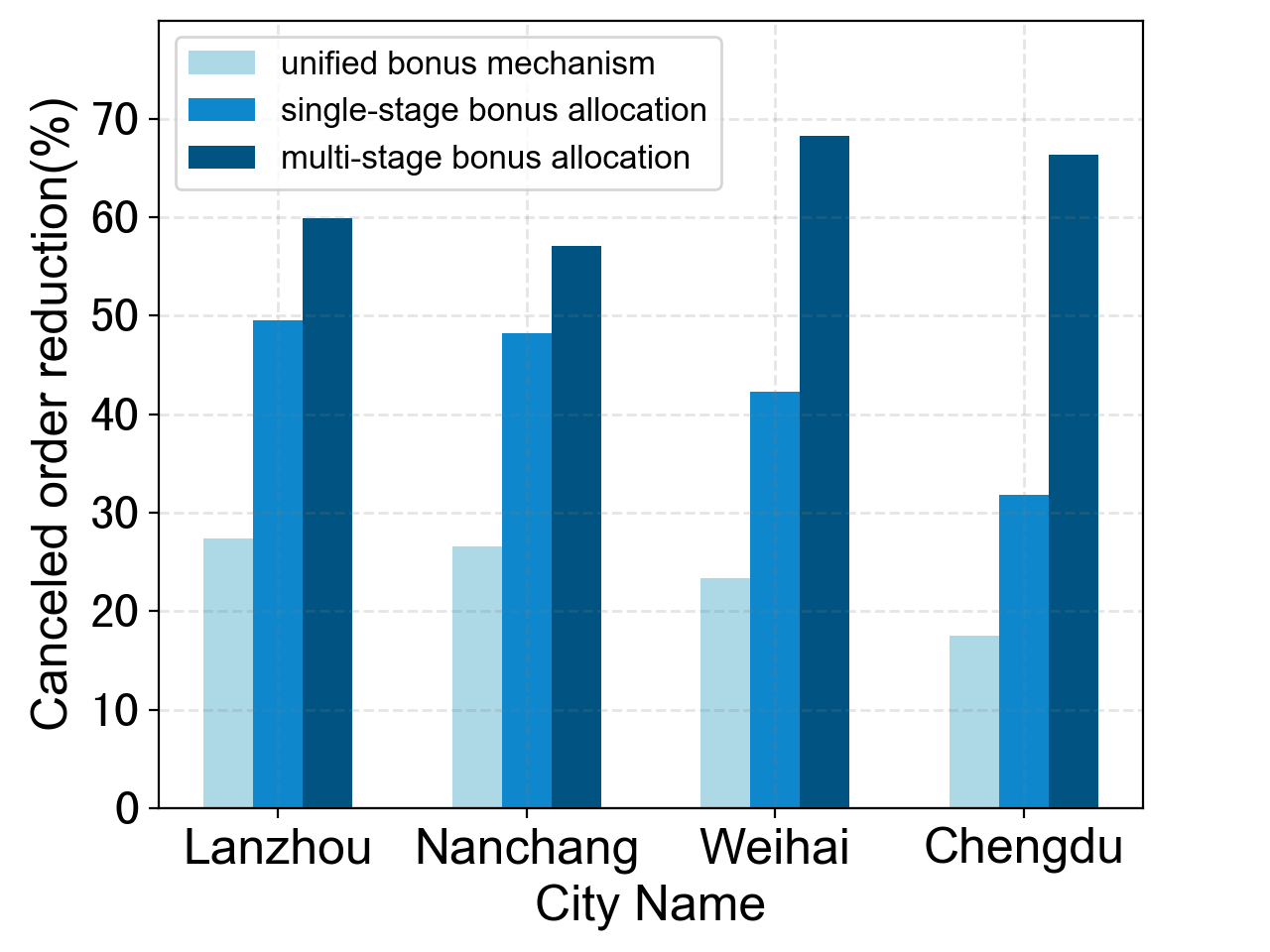
(a)

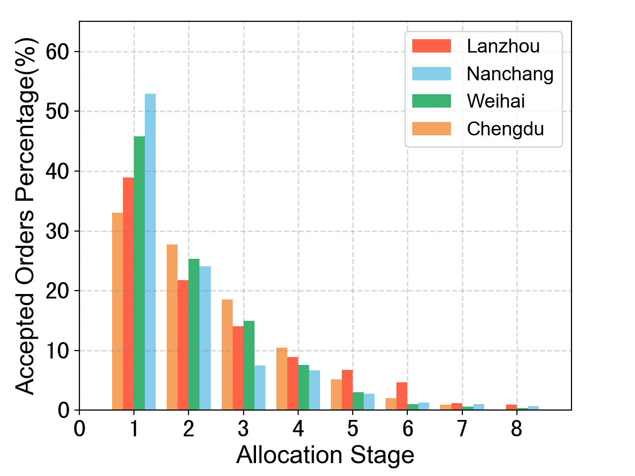
(b)

Figure 8. (a) Comparison of the canceled order reduction with different approaches. (b) The number of accepted orders on multiple allocation stages.

4.1.2. Performance of bonus allocation methods with different budget

In this section, we analyze the performance of bonus allocation methods with different budgets. We compare the results derived by the MSBA ,the single-stage allocation and the unified bonus mechanism when the budget changes. Figure 9 reflects the relationship between the budget and the number of NA-canceled order. The MSBA method outperforms the single-stage allocation and the unified bonus mechanism. Particularly, with a small budget, the MSBA method performs much better than the single-stage allocation and the unified bonus mechanism . As the budget becomes more and more sufficient, the budget can cover all potential cancel orders, while the rest could not be solved by algorithms. Hence the three algorithms get converged under a larger budget.

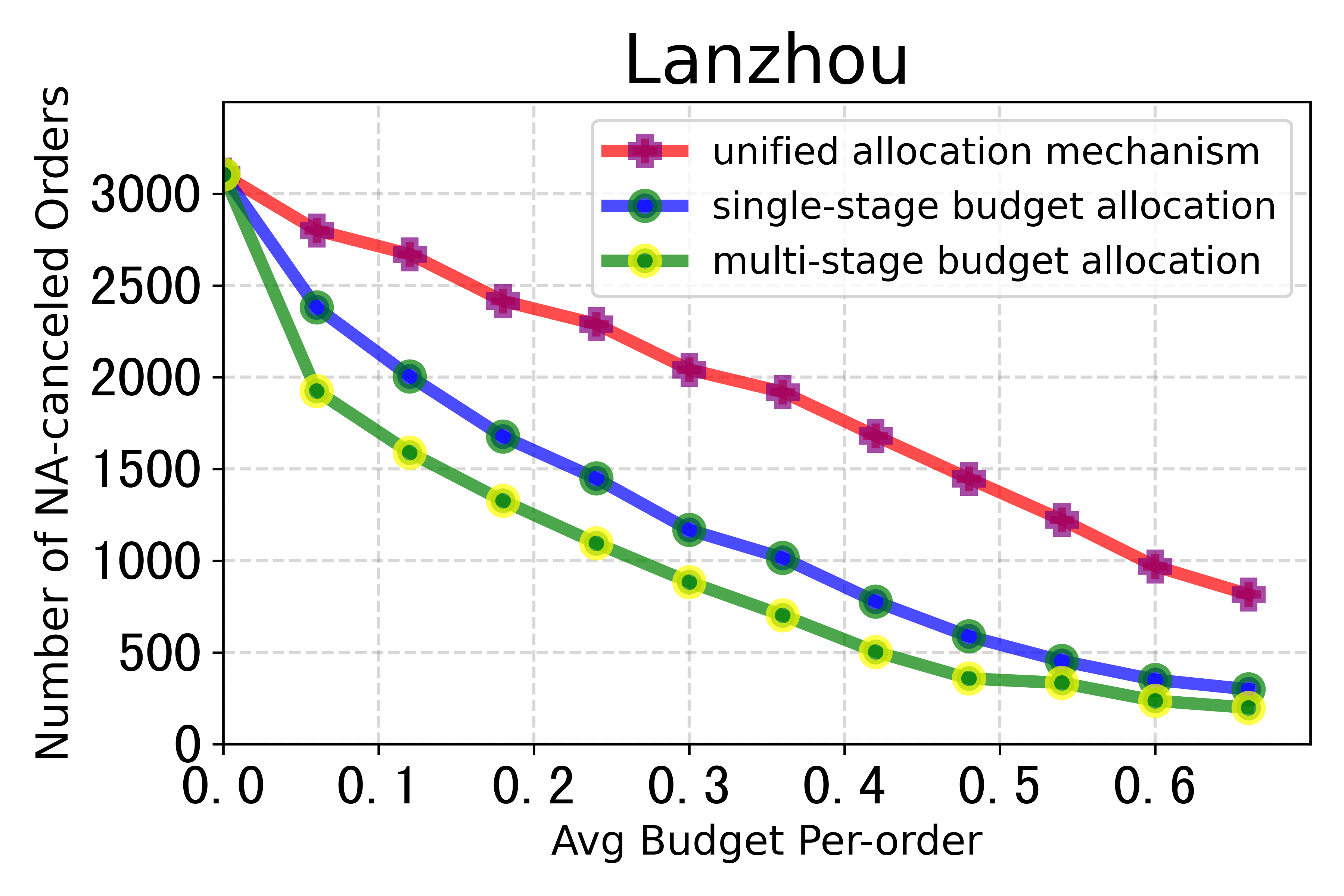
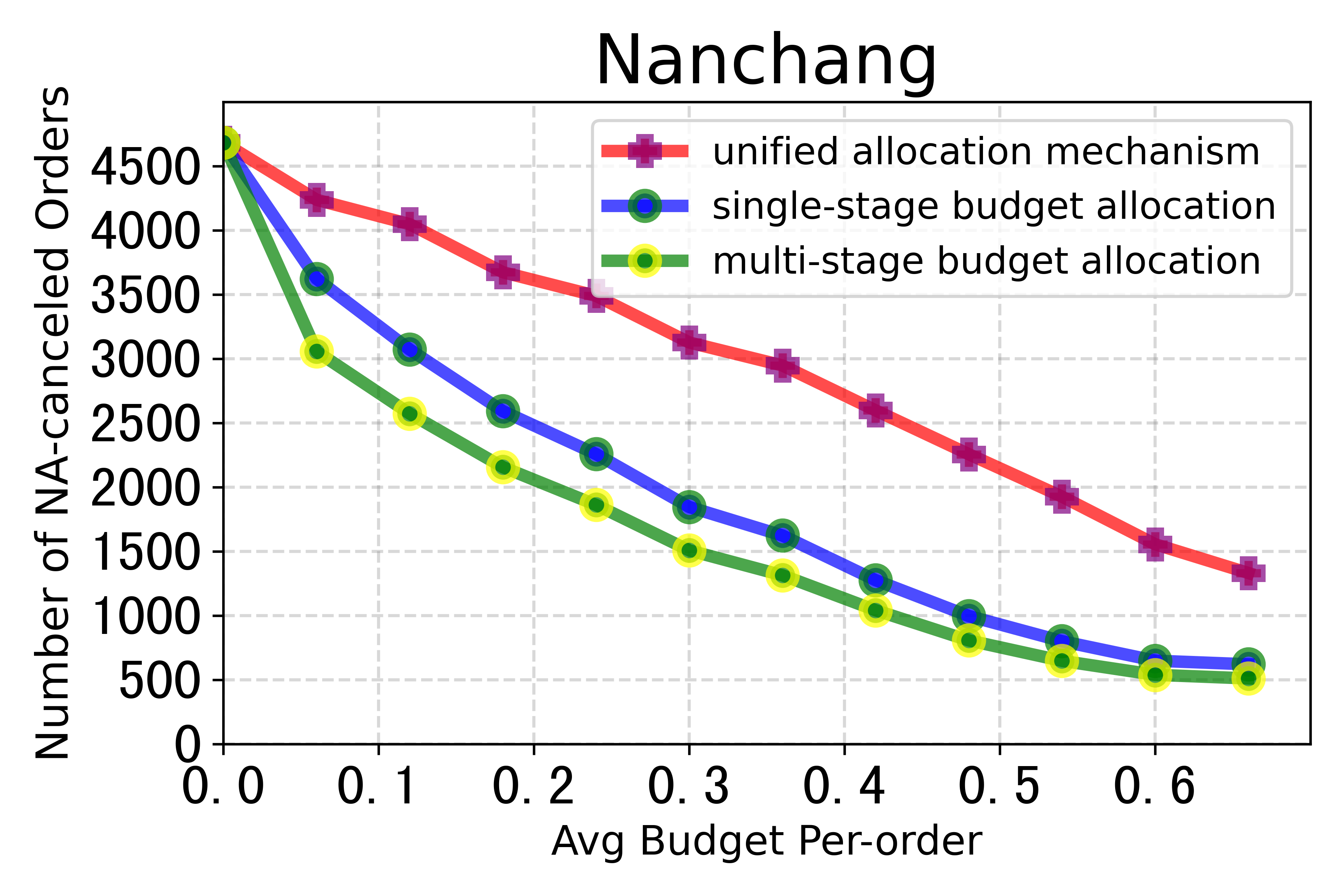
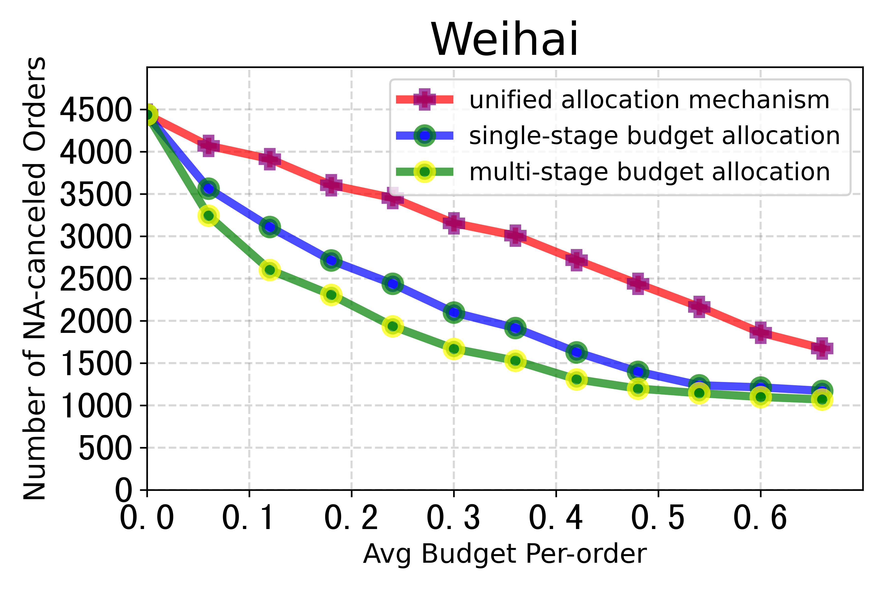
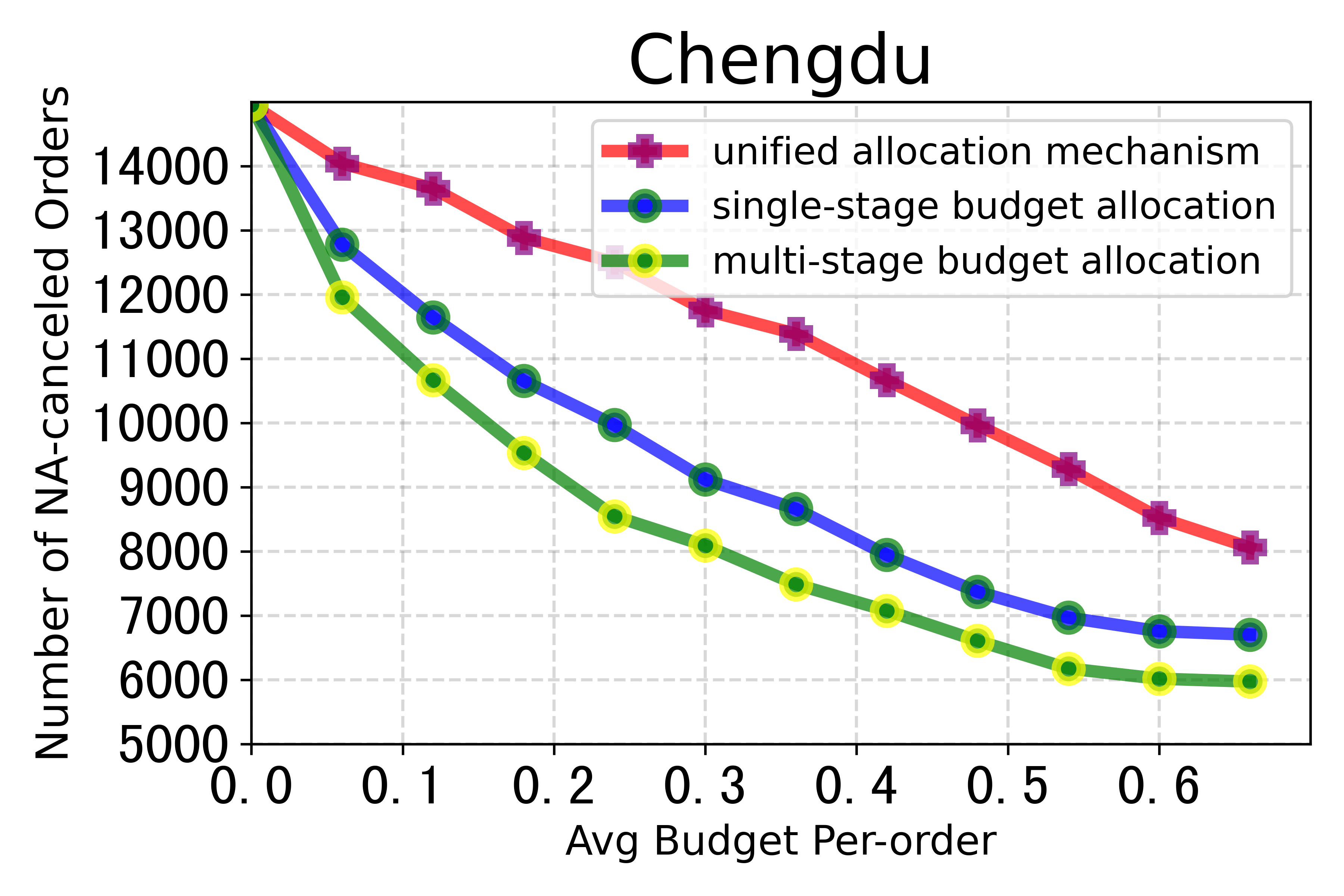
Figure 9. Comparison of the NA-canceled order reduction with different approaches at diffent budget.

4.1.3. Impact of the number of the allocation stages

This section investigates the impact of the number of the allocation stages on the accepted order quantity. As shown in Figure 10, the accepted order quantity increases when the number of allocation stages increases. However, the slope of the curve becomes smaller when the number of allocation stages is more than 10. Besides, it is detrimental to the crowdsourcing driver experiences that the delivery bonus of an order changes too frequently. Therefore, to balance the accepted order quantity and the crowdsourcing driver experience, it is reasonable to set the allocation stages no more than 10.

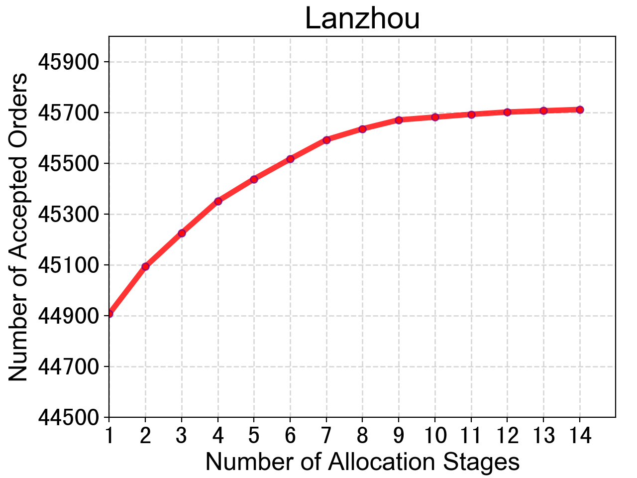
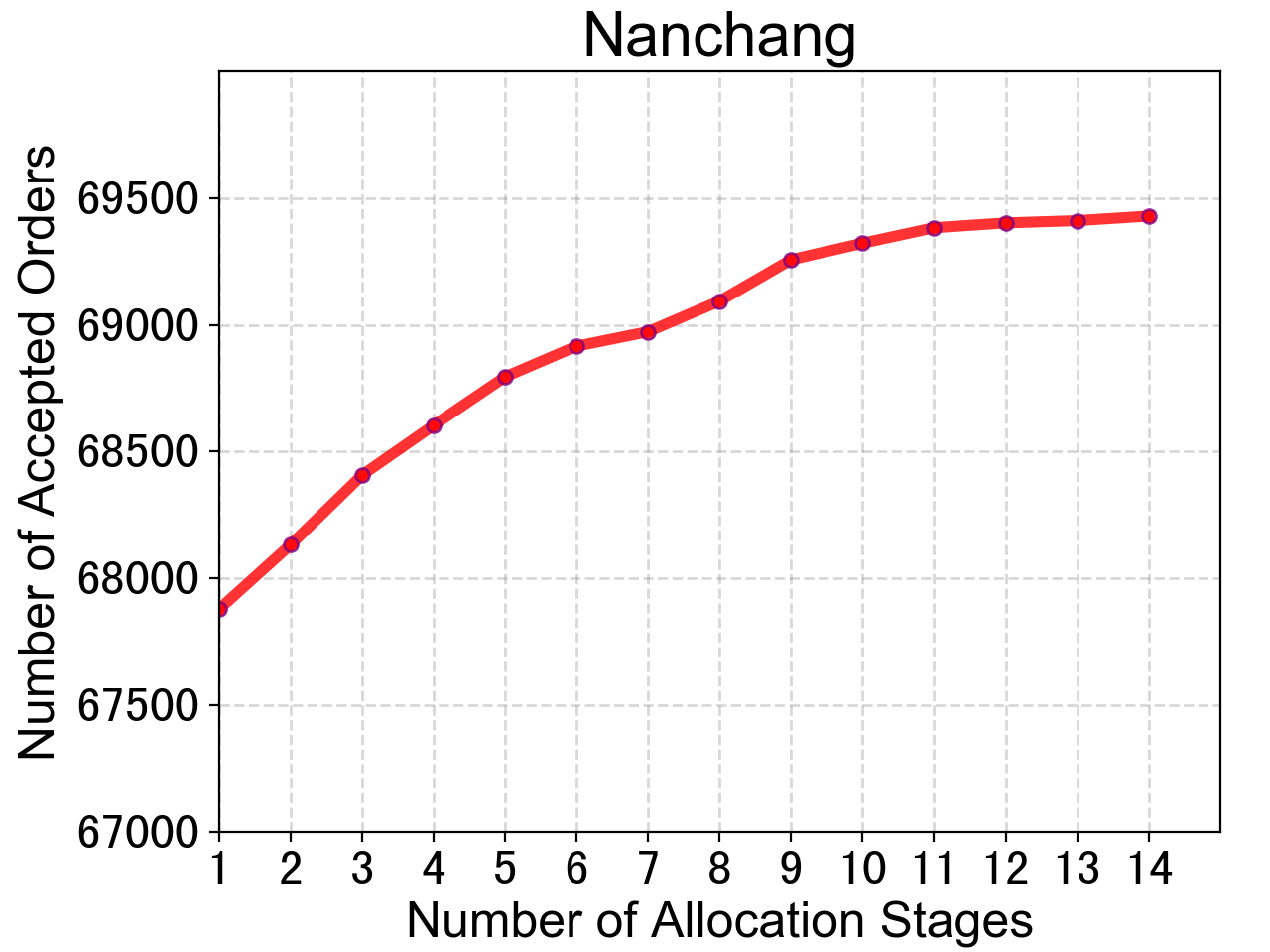
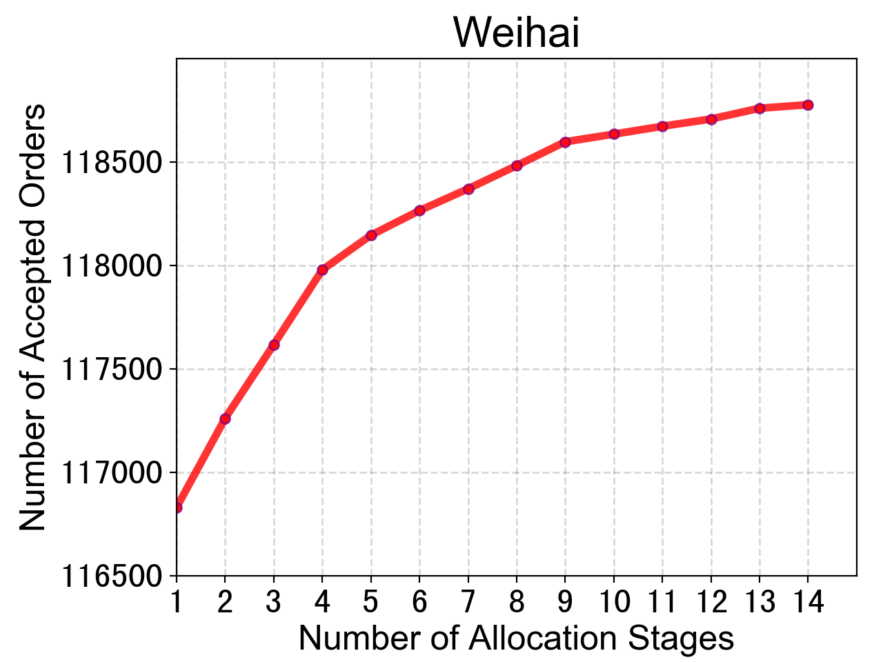
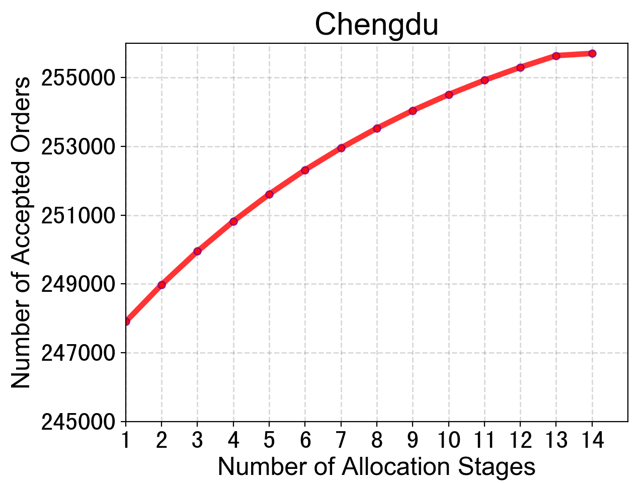
Figure 10. Impact of the number of the allocation stages on the number of accepted orders.

4.2. Performance of online A/B tests

In this section, we introduce our online A/B tests on the Meituan meal delivery platform.

We implemented our A/B tests on five cities in China, covering 120 delivery areas and 4,960,000 orders per day. The orders are randomly and equally split to 3 groups, adopting multi-stage, single-stage and unified allocation method separately. The budget for both the experimental and control group is set to 0.2 RMB per order. To verify the effectiveness of our algorithm, we recorded the order information data two weeks before and after the start of the experiment for both groups. We employ the LDDP algorithm to calculate the Lagrangian multiplier for each allocation stage by the historical data set 30 days before the experiment. The empirical Lagrangian multipliers are updated every day. The online allocation algorithm is triggered when an order is presented on the screen of the crowdsourcing driver. The delivery bonus of an order is calculated in milliseconds using the empirical Lagrangian multiplier.

Table 1. Performance of online A/B tests.

City Name	Multi-Stage Bonus Allocation				Single-Stage Bonus Allocation		Unified Bonus Allocation
	NA-canceled ratio	drops% v.s. single-stage	drops% v.s. unified	per-order compensation	NA-canceled ratio	per-order compensation	NA-canceled ratio	per-order compensation
Nanchang	0.68 %	38.47%	60.82%	0.0049	1.11%	0.0078	1.74%	0.0086
Shenzhen	0.49%	31.70%	51.62%	0.0038	0.72%	0.0057	1.01%	0.0073
Weihai	0.81%	27.51%	40.00%	0.0056	1.12%	0.0078	1.35%	0.0098
Zhuhai	0.56%	27.06%	32.76%	0.0038	0.77%	0.0050	0.84%	0.0061
Shantou	1.56%	25.02%	29.83%	0.0073	2.09%	0.0101	2.23%	0.0113

The results are evaluated from two aspects: the NA-canceled order ratio and the compensation paid to restaurants for food waste per order (in RMB), which are two important indicators to the platform. As shown in Table 1, using the proposed method, compared to the single-stage allocation method the NA-canceled orders ratio was reduced by more than 25%, and more than 29% compared to the unified allocation method under the same budget. Furthermore, we can save more than 30% of the compensation paid to restaurants for food waste.

5. Related Work

Some studies have studied dynamic pricing for attended home delivery (Klein et al., 2018; Koch and Klein, 2020; Yang et al., 2016) where time slot pricing was implemented to dynamically affect customers’ bookings using approximate dynamic programming. (Yang et al., 2016) proposed approximating the opportunity cost by calculating the insertion cost of an incoming request based on the insertion heuristic algorithm. Klein et al.(Klein et al., 2018) improved the method of Yang et al. by considering expected future demand, making delivery cost approximation more accurate. Koch et al. (Koch and Klein, 2020) combine and extend the methods in the previous paper by considering more flexible customer choice and dynamic vehicle routing with time windows. Ulmer (Ulmer, 2020) established a Markov decision process model for dynamic routing and same-day delivery pricing and presented an anticipatory pricing method to solve it. Based on this work of Ulmer (Ulmer, 2020), Prokhorchuk et al. (Prokhorchuk et al., 2019) considered a stochastic travel time to make the model more applicable. Some references discussed the researches related to the meal delivery problem(Yildiz and Savelsbergh, 2019; Ulmer et al., 2021; Ding et al., 2020), but few of them involved the pricing and bonus allocation problem.

There are some studies on dynamic pricing for ride-hailing platforms. Some ride-hailing platforms use a dynamic pricing strategy called surge/prime pricing, in which the base fare is multiplied by a multiplier that is greater than one when the demand is high relative to supply (Hall et al., 2015). Castillo et al.(Castillo et al., 2017) proposed a steady-state model for dynamic pricing in ride-hailing applications and validated that dynamic pricing is particularly important for ride-hailing owing to the so-called wild ”goose chase phenomenon”. Zha et al.(Zha et al., 2018) built a spatial pricing model based on a discrete-time geometric matching framework in which a customer is matched to their closest available vehicle within a set radius. Tong et al. (Tong et al., 2018) proposed the Global Dynamic Pricing (GDP) in spatial crowdsourcing in a ride-hailing platform context. It proposes dynamic pricing in multiple local markets with unknown demand, limited supply, or dependent supply. It differs in pricing between ride-hailing and meal delivery problems. For example, dynamic pricing for ride-hailing determines the price presented to passengers spatiotemporally, but a delivery bonus is presented to drivers based on the order features for meal delivery.

6. Conclusion

In this paper, we study the MSBA problem for meal delivery platform. We propose a framework including a semi-black-box acceptance probability model, an LDDP algorithm, and an online allocation algorithm to solve this problem. Using this framework, online decision could be made within milliseconds. Both offline experiments and online A/B tests are implemented to verify the effectiveness of our method. The offline experiments show that compared to single-stage bonus allocation and unified bonus mechanism, the number of canceled orders derived from MSBA decrease about 25% and 50%, respectively. The online A/B tests show that compared to single-stage bonus allocation the number of canceled orders reduced by more than 25%. The proposed algorithm has been actually applied in the largest meal delivery platform in China.

References

- (1)
- Birge (1985) John R Birge. 1985. Decomposition and partitioning methods for multistage stochastic linear programs. Operations research 33, 5 (1985), 989–1007.
- Boyd et al. (2004) Stephen Boyd, Stephen P Boyd, and Lieven Vandenberghe. 2004. Convex optimization. Cambridge university press.
- Castillo et al. (2017) Juan Camilo Castillo, Dan Knoepfle, and Glen Weyl. 2017. Surge pricing solves the wild goose chase. In Proceedings of the 2017 ACM Conference on Economics and Computation. 241–242.
- Chen et al. (2015) Tianqi Chen, Tong He, Michael Benesty, Vadim Khotilovich, Yuan Tang, Hyunsu Cho, et al. 2015. Xgboost: extreme gradient boosting. R package version 0.4-2 1, 4 (2015), 1–4.
- Ding et al. (2020) Xuetao Ding, Runfeng Zhang, Zhen Mao, Ke Xing, Fangxiao Du, Xingyu Liu, Guoxing Wei, Feifan Yin, Renqing He, and Zhizhao Sun. 2020. Delivery Scope: A New Way of Restaurant Retrieval for On-demand Food Delivery Service. In Proceedings of the 26th ACM SIGKDD International Conference on Knowledge Discovery & Data Mining. 3026–3034.
- Dong et al. (2009) Lingxiu Dong, Panos Kouvelis, and Zhongjun Tian. 2009. Dynamic pricing and inventory control of substitute products. Manufacturing & Service Operations Management 11, 2 (2009), 317–339.
- Hall et al. (2015) Jonathan Hall, Cory Kendrick, and Chris Nosko. 2015. The effects of Uber’s surge pricing: A case study. The University of Chicago Booth School of Business (2015).
- Hao et al. (2015) Jinghua Hao, Min Liu, Shenglong Jiang, and Cheng Wu. 2015. A soft-decision based two-layered scheduling approach for uncertain steelmaking-continuous casting process. European Journal of Operational Research 244, 3 (2015), 966–979.
- Klein et al. (2018) Robert Klein, Jochen Mackert, Michael Neugebauer, and Claudius Steinhardt. 2018. A model-based approximation of opportunity cost for dynamic pricing in attended home delivery. OR Spectrum 40, 4 (2018), 969–996.
- Koch and Klein (2020) Sebastian Koch and Robert Klein. 2020. Route-based approximate dynamic programming for dynamic pricing in attended home delivery. European Journal of Operational Research (2020).
- Li and Huh (2011) Hongmin Li and Woonghee Tim Huh. 2011. Pricing multiple products with the multinomial logit and nested logit models: Concavity and implications. Manufacturing & Service Operations Management 13, 4 (2011), 549–563.
- Prokhorchuk et al. (2019) Anatolii Prokhorchuk, Justin Dauwels, and Patrick Jaillet. 2019. Stochastic Dynamic Pricing for Same-Day Delivery Routing. arXiv preprint arXiv:1912.02946 (2019).
- Si et al. (2004) Jennie Si, Andrew G Barto, Warren B Powell, and Don Wunsch. 2004. Handbook of learning and approximate dynamic programming. Vol. 2. John Wiley & Sons.
- Tong et al. (2018) Yongxin Tong, Libin Wang, Zimu Zhou, Lei Chen, Bowen Du, and Jieping Ye. 2018. Dynamic pricing in spatial crowdsourcing: A matching-based approach. In Proceedings of the 2018 International Conference on Management of Data. 773–788.
- Ulmer (2020) Marlin W Ulmer. 2020. Dynamic pricing and routing for same-day delivery. Transportation Science 54, 4 (2020), 1016–1033.
- Ulmer et al. (2021) Marlin W Ulmer, Barrett W Thomas, Ann Melissa Campbell, and Nicholas Woyak. 2021. The Restaurant Meal Delivery Problem: Dynamic Pickup and Delivery with Deadlines and Random Ready Times. Transportation Science 55, 1 (2021), 75–100.
- Wolsey (1998) Laurence A Wolsey. 1998. Integer programming. Vol. 52. John Wiley & Sons.
- Yang and Huang (2001) XQ Yang and XX Huang. 2001. A nonlinear Lagrangian approach to constrained optimization problems. SIAM Journal on Optimization 11, 4 (2001), 1119–1144.
- Yang et al. (2016) Xinan Yang, Arne K Strauss, Christine SM Currie, and Richard Eglese. 2016. Choice-based demand management and vehicle routing in e-fulfillment. Transportation science 50, 2 (2016), 473–488.
- Yildiz and Savelsbergh (2019) Baris Yildiz and Martin Savelsbergh. 2019. Provably high-quality solutions for the meal delivery routing problem. Transportation Science 53, 5 (2019), 1372–1388.
- Zha et al. (2018) Liteng Zha, Yafeng Yin, and Zhengtian Xu. 2018. Geometric matching and spatial pricing in ride-sourcing markets. Transportation Research Part C: Emerging Technologies 92 (2018), 58–75.
- Zhao et al. (2019) Kui Zhao, Junhao Hua, Ling Yan, Qi Zhang, Huan Xu, and Cheng Yang. 2019. A Unified Framework for Marketing Budget Allocation. In Proceedings of the 25th ACM SIGKDD International Conference on Knowledge Discovery & Data Mining. 1820–1830.