On the stability of nonlinear sampled-data systems and their continuous-time limits

Abstract

This work deals with the stability analysis of nonlinear sampled-data systems under nonuniform sampling. It establishes novel relationships between the stability property of the exact discrete-time model for a given sequence of (aperiodic) sampling instants and the stability property of the continuous-time system when the maximum admissible sampling period converges to zero. These results can be used to infer stability properties for the sampled-data system by direct inspection of the stability of the mentioned continuous-time system, a task which is typically easier than the analysis of the closed-loop sampled-data system. Compared to the literature, our results allow to prove stronger (asymptotic) sampled-data stability properties for nonlinear systems in cases for which existing results only guarantee practical stability.

1 Introduction

The two main approaches to design controllers for sampled-data nonlinear systems are: a) to design a discrete-time (DT) controller based on a DT model of the plant [Nešić et al., 1999, Nešić and Teel, 2004, Liu et al., 2008, Nešić et al., 2009a, Üstüntürk, 2012, Üstüntürk and Kocaoğlan, 2013, Noroozi et al., 2018, Beikzadeh et al., 2018, Vallarella and Haimovich, 2019] or b) to obtain the controller by adequate discretization of a continuous-time (CT) one. In the first approach, the DT model is usually an approximation due to the impossibility of solving nonlinear differential equations in closed form. In the second approach, emulation of the CT controller is known to stabilize the sampled/data system under sufficiently fast sampling [Nešić et al., 2009b, Proskurnikov, 2020]. In addition, controller redesign that accounts for sampling may lead to better performance [Nešić and Grüne, 2005, Monaco and Normand-Cyrot, 2007, Grüne et al., 2008, Postoyan et al., 2008]. In both approaches, the final result is in general a sampling period/dependent DT control law to be implemented usually under zero-order hold.

Results along the first approach generally give conditions under which a stability property of the approximate DT model in closed loop is enough to guarantee (some type of) stability of the closed-loop sampled-data system under sufficiently fast sampling. In many cases, only practical (not asymptotic) stability is ensured or else strong conditions are imposed [see Vallarella et al., 2021, and references therein]. Uniform (periodic) sampling is usually considered, but some results ensuring only practical stability also allow nonuniform (aperiodic) sampling [Di Ferdinando and Pepe, 2019, Di Ferdinando et al., 2021]. Works that address asymptotic stability of sampled-data systems and do not fall within any of the two approaches mentioned also exist [Li and Zhao, 2018, Lin and Wei, 2018, Lin, 2020, Lin and Sun, 2021]. Li and Zhao [2018] shows how asymptotic stability can be preserved via the selection of a specific sampling period. Lin and Wei [2018], Lin [2020], Lin and Sun [2021] give results for semiglobal asymptotic stabilizability under constant sampling, where the term “semiglobal” involves possibly different convergence rates for different sets of initial conditions and upper bounds on the sampling period. By contrast, previous own works within the first approach [Vallarella and Haimovich, 2019, 2018, Vallarella et al., 2021] address semiglobal stability properties, where “semiglobal” involves the same convergence rate but possibly different maximum sampling periods for every initial condition, and allow nonuniform sampling [Omran et al., 2016, Hetel et al., 2017]. In particular, we derived conditions under which semiglobal (practical or exponential) stability is carried over between different DT models [Vallarella and Haimovich, 2019, Vallarella et al., 2021] and we provided adequate Lyapunov-type guarantees [Vallarella and Haimovich, 2018]. This allows to establish the stability of the exact DT model, i.e. the model whose state coincides with the state of the sampled/data system at sampling instants and which is not assumed to be available.

In this context, the aim of this note is to establish a precise correspondence between asymptotic (not only practical) stability properties under nonuniform sampling of the exact DT model and stability properties of a related CT system. This CT system is just the CT open-loop system in closed-loop with the CT limit of the control law, the latter being the value of the control action when the sampling period tends to zero. We provide mild conditions on the open-loop models and (sampling period/dependent) control laws under which the closed-loop exact DT model exhibits some asymptotic stability property if and only if the related CT system exhibits the respective CT equivalent property. These conditions complement existing results by allowing to guarantee stronger (asymptotic) stability properties for the sampled/data system in cases where previous results only show practical stability or apply to uniform sampling. The mild conditions required admit systems that are not globally Lipschitz and not necessarily input-affine, and control laws that may be not differentiable with respect to the sampling period.

Notation: $\mathbb{R}$, $\mathbb{R}_{\geq 0}$, $\mathbb{N}$ and $\mathbb{N}_{0}$ denote the reals, nonnegative reals, naturals and nonnegative integers. Classes $\mathcal{K}$, $\mathcal{K}_{\infty}$ and $\mathcal{KL}$ of functions are defined as in Khalil [2002]. For a vector $x\in\mathbb{R}^{n}$, $|x|$ denotes its Euclidean norm. A sequence is noted as $\{T_{i}\}:=\{T_{i}\}_{i=0}^{\infty}$. For any $\{T_{i}\}\subset\mathbb{R}_{\geq 0}$, we define $\sum_{i=0}^{-1}T_{i}=0$. Given $T>0$, we define $\Phi(T):=\{\{T_{i}\}:\{T_{i}\}\text{ is such that }T_{i}\in(0,T)\text{ for all }i\in\mathbb{N}_{0}\}$.

2 Problem statement

Our aim is to obtain mild conditions that preserve stability properties for sampled-data systems that arise from nonlinear plants of the form

$$\dot{x}=f(x,u),$$ (1)

under zero-order hold, where $x(t)\in\mathbb{R}^{n}$, $u(t)\in\mathbb{R}^{m}$ are the state and control vectors. A control law $u_{c}:\mathbb{R}^{n}\rightarrow\mathbb{R}^{m}$ may render

$$\dot{x}=f(x,u_{c}(x))=:h(x)$$ (2)

stable as per one of the following definitions.

Definition 2.1.

The system (2) is said to be

1. Globally Asymptotically Stable (GAS) if there exists $\beta\in\mathcal{KL}$ such that for any $x_{0}\in\mathbb{R}^{n}$ the solutions satisfy $|x(t)|\leq\beta(|x_{0}|,t),\medspace\forall t\geq 0$. If additionally $\beta\in\mathcal{KL}$ can be chosen as $\beta(r,t):=Kre^{-\lambda t}$ with $K\geq 1$ and $\lambda>0$ it is said to be Globally Exponentially Stable (GES).

2. Locally Exponentially Stable (LES) if there exist $K\geq 1$ and $R,\lambda>0$ such that for all $|x_{0}|\leq R$ the solutions satisfy $|x(t)|\leq K|x_{0}|e^{-\lambda t},\medspace\forall t\geq 0$.

3. GALES if it is GAS and LES.

We consider that the function $f$ in (1) and a control law $u_{c}$ in (2) fulfill the following local Lipschitzness assumptions.

Assumption 2.2.

$f:\mathbb{R}^{n}\times\mathbb{R}^{m}\rightarrow\mathbb{R}^{n}$ fulfills $f(0,0)=0$ and for every $M,M_{u}\geq 0$ there exists $L=L(M,M_{u})>0$ such that for all $|x|,|y|\leq M$ and $|u|,|v|\leq M_{u}$ we have $\left|f(x,u)-f(y,v)\right|\leq L(|x-y|+|u-v|)$.

Assumption 2.3.

$u_{c}:\mathbb{R}^{n}\rightarrow\mathbb{R}^{m}$ fulfills $u_{c}(0)=0$ and for every $M\geq 0$ there exists $L=L(M)>0$ such that for all $|x|,|y|\leq M$ we have $\left|u_{c}(x)-u_{c}(y)\right|\leq L|x-y|$.

We consider sampling instants $t_{k}$, $k\in\mathbb{N}_{0}$, $t_{0}=0$ and $t_{k+1}=t_{k}+T_{k}$, where $T_{k}>0$ is the $k^{th}$ sampling period. The sampling periods may vary following any possible sequence as long as they are bounded by a maximum admissible sampling interval; we refer to this situation as Varying Sampling Rate (VSR). We assume that $T_{k}$ is either known or determined at instant $t_{k}$, so that this information may be used to perform the current control action: $u_{k}=U(x_{k},T_{k})$. This is always the case under periodic sampling (i.e. $T_{k}\equiv T>0$), where the control law is designed based on prior knowledge of the sampling period. The sampled/data system that arises from (1) in feedback with $u_{k}=U(x_{k},T_{k})$ under zero-order hold is

$$\dot{x}(t)=f(x(t),U(x(t_{k}),T_{k}))\text{ }\medspace\forall t\in[t_{k},t_{k+1}),\medspace k\in\mathbb{N}_{0}.$$ (3)

We consider DT models of (3). These can be regarded as estimates of the value $x_{k+1}=x(t_{k+1})$, given $x_{k}$ and $u_{k}$ at the sampling instant $t_{k}$, namely $x_{k+1}=F(x_{k},u_{k},T_{k})$. The exact DT model is the one that generates the actual value that $x(t_{k+1})$ will have as the solution of (3), and is denoted by $F^{e}$. For nonlinear plants, the exact DT model may be unavailable due to the difficulty or impossibility of solving nonlinear differential equations. Thus, a suitable design approach is to design the control law based on a sufficiently good approximate DT model of the plant, such as Runge-Kutta models [Stuart and Humphries, 1996]. The simplest of these models, the Euler model, is given by $F^{E}(x,u,T):=x+Tf(x,u)$. For a DT model $F$ and control law $U$, we define the closed-loop DT model $\bar{F}_{U}(x,T):=F(x,U(x,T),T)$. We may also simply denote a closed-loop DT model by $\bar{F}$ when the control law is not important in the context.

To state our results we need the following Equilibrium/Preserving Consistency (EPC) property, which bounds the mismatch between any two of the previously defined DT models’ solutions after one sampling interval. This property becomes equivalent to the REPC property in Vallarella et al. [2021] when no errors affect the control input.

Definition 2.4.

The DT model $\bar{F}^{a}$ is said to be Equilibrium/Preserving Consistent (EPC) with $\bar{F}^{b}$ if for each $M\geq 0$ there exist constants $K:=K(M)>0$, $T^{*}:=T^{*}(M)>0$ and a function $\rho\in\mathcal{K}_{\infty}$ such that

$$\left|\bar{F}^{a}(x,T)-\bar{F}^{b}(y,T)\right|\leq(1+KT)\left|x-y\right|+T\rho(T)\max\{|x|,|y|\}$$ (4)

for all $|x|,|y|\leq M$ and $T\in(0,T^{*})$. The pair $(\bar{F}^{a},\bar{F}^{b})$ is said to be EPC if $\bar{F}^{a}$ is EPC with $\bar{F}^{b}$.

The EPC property is sufficient to ensure that the following stability properties for DT models, suitable under nonuniform sampling [see Vallarella and Haimovich, 2019, 2018, Vallarella et al., 2021], are shared between different DT models. This fact is stated in Theorem 2.6.

Definition 2.5.

The system $x_{k+1}=\bar{F}(x_{k},T_{k})$ is said to be

1. Semiglobally Practically Stable-VSR (SPS-VSR) if there exists $\beta\in\mathcal{KL}$ such that for every $M\geq 0$ and $R>0$ there exists $T^{\star}:=T^{\star}(M,R)>0$ such that for all $k\in\mathbb{N}_{0}$, $\{T_{i}\}\in\Phi(T^{\star})$ and $|x_{0}|\leq M$ the solutions satisfy $|x_{k}|\leq\beta\left(|x_{0}|,\sum_{i=0}^{k-1}T_{i}\right)+R$.

2. Locally Exponentially Stable-VSR (LES-VSR) if there exist $K\geq 1$ and $R,T^{\star},\lambda>0$ such that for all $k\in\mathbb{N}_{0}$, $\{T_{i}\}\in\Phi(T^{\star})$ and $|x_{0}|\leq R$ the solutions satisfy $|x_{k}|\leq K|x_{0}|e^{-\lambda\sum_{i=0}^{k-1}T_{i}}$.

3. Semiglobally (asymptotically) and Locally Exponentially Stable (SLES-VSR) if it is SPS-VSR and LES-VSR.

4. Semiglobally (asymptotically) Stable-VSR (SS-VSR) if there exists $\beta\in\mathcal{KL}$ such that for every $M\geq 0$ there exists $T^{\star}:=T^{\star}(M)>0$ such that for all $k\in\mathbb{N}_{0}$, $\{T_{i}\}\in\Phi(T^{\star})$ and $|x_{0}|\leq M$ the solutions satisfy $|x_{k}|\leq\beta\left(|x_{0}|,\sum_{i=0}^{k-1}T_{i}\right)$. If additionally $\beta\in\mathcal{KL}$ can be chosen as $\beta(r,t):=Kr\exp(-\lambda t)$ with $K\geq 1$ and $\lambda>0$ it is said to be Semiglobally Exponentially Stable-VSR (SES-VSR).

Theorem 2.6.

Suppose that $(\bar{F}^{a},\bar{F}^{b})$ is EPC. Then i) $\bar{F}^{a}$is SPS-VSR $\Leftrightarrow$ $\bar{F}^{b}$ is SPS-VSR. ii) $\bar{F}^{a}$is LES-VSR $\Leftrightarrow$ $\bar{F}^{b}$ is LES-VSR. iii) $\bar{F}^{a}$is SLES-VSR $\Leftrightarrow$ $\bar{F}^{b}$ is SLES-VSR.

The proof of Theorem 2.6 follows from the proofs of Vallarella et al. [2021, Theorem 3.5, Lemma 3.7] and Vallarella and Haimovich [2019, Theorem 3.1], imposing that no errors affect the control input and can be found in Section 6. To establish that an approximate model $F^{a}$ in closed loop with a control law $U(x,T)$ is such that $\bar{F}^{a}_{U}$ is EPC with the exact model $\bar{F}^{e}_{U}$, one could prove EPC of $(\bar{F}^{E}_{U},\bar{F}^{a}_{U})$, with $\bar{F}^{E}$ the Euler model, which is much simpler. This is all that is required because EPC is a transitive property and $(\bar{F}^{e}_{U},\bar{F}^{E}_{U})$ is already known to be EPC [Vallarella et al., 2021]. Once $(\bar{F}^{a}_{U},\bar{F}^{e}_{U})$ EPC is established, application of Theorem 2.6 would ensure that a stability property of the approximate model also holds for the exact model.

3 Main results

In this section, we present mild sufficient conditions under which sampled-data stability properties as per Definition 2.5 hold if and only if the closed-loop CT system (2), with $u_{c}$ equal to a specific limit of the DT control law, has a corresponding stability property. Conditions to ensure that different open-loop models (say $F^{a}$ and $F^{b}$) in closed/loop with the same control law (say $U$), are EPC, i.e. $(\bar{F}^{a}_{U},\bar{F}^{b}_{U})$ is EPC, already exist [Vallarella et al., 2021]. To derive our main results we need an extension to the case where different control laws may be used, for which we require the following consistency and regularity conditions.

Definition 3.1.

The pair $(U,V)$ is said to be Semiglobally small-time convergent Consistent (StC) if for each $M\geq 0$ there exist a function $\rho\in\mathcal{K}_{\infty}$ and $T^{*}:=T^{*}(M)>0$ such that for all $|x|\leq M$ and $T\in[0,T^{*})$ we have

$$|U(x,T)-V(x,T)|\leq\rho(T)|x|.$$ (5)

Definition 3.2.

The function $U$ is said to be Semiglobally small-time Lipschitz (StL) if for each $M\geq 0$ there exist $K:=K(M)>0$, $T^{*}:=T^{*}(M)>0$ with $T^{*}(\cdot)$ nonincreasing such that for all $|x|,|y|\leq M$ and $T\in[0,T^{*})$ we have $U(0,T)=0$ and

$$|U(x,T)-U(y,T)|\leq K|x-y|.$$ (6)

Definition 3.3.

The DT model $F^{a}$ is said to be Semiglobally small-time Lipschitz Consistent (StLC) if for each $M,E\geq 0$ there exist $K:=K(M,E)>0$, $T^{*}:=T^{*}(M,E)>0$ such that for all $|x|,|y|\leq M$, $|u|,|v|\leq E$, and $T\in[0,T^{*})$

$$|F^{a}(x,u,T)-F^{a}(y,v,T)|\leq(1+KT)|x-y|+KT|u-v|.$$ (7)

Theorem 3.4 gives sufficient conditions so that closed-loop models arising from feeding back the same open-loop model with different control laws are EPC. Theorems 2.6 and 3.4 are both needed to prove Theorem 3.5, which is our main result. The proofs of Theorems 3.4 and 3.5 are provided in Section 6.

Theorem 3.4 (Proof in Section 6.2).

Suppose that i) $F^{a}$is StLC, ii) $U$is StL, iii) $(U,V)$is StC. Then $(\bar{F}^{a}_{U},\bar{F}^{a}_{V})$ is EPC.

Theorem 3.5 (Proof in Section 6.3).

Consider system (1), a DT control law $U(x,T)$, and the CT control law $u_{c}(x):=U(x,0)$. Suppose that

1. Assumptions 2.2 and 2.3 hold.

2. $U$ is StL.

3. $(U,U_{c})$ is StC, with $U_{c}(x,T):=u_{c}(x)$ for all $T\geq 0$.

Then the CT closed/loop plant (2) is

1. GALES $\Leftrightarrow$ the exact model $\bar{F}^{e}_{U}$ is LES-VSR.

2. GALES $\Leftrightarrow$ the exact model $\bar{F}^{e}_{U}$ is SLES-VSR.

3. ALGES $\Leftrightarrow$ the exact model $\bar{F}^{e}_{U}$ is SES-VSR.

Previous results ensure that semiglobal practical [Nešić et al., 1999, Vallarella and Haimovich, 2019] or semiglobal exponential [Vallarella et al., 2021] stability exhibited by an approximate open/loop model $F^{a}$ in closed/loop with a control law $U(x,T)$ is carried over to the exact closed/loop model $\bar{F}^{e}_{U}$. By Theorem 3.5 it may be possible to establish even stronger stability properties of the same exact model $\bar{F}^{e}_{U}$ by analyzing the stability of the CT system (2) in closed/loop with the CT limit of $U$, i.e. $u_{c}(x):=U(x,0)$. For example, it is known that (2) is LES if and only if its linearization at the equilibrium is GES. If $\bar{F}^{e}_{U}$ is already known to be SPS-VSR, and (2) is LES, then according to Theorem 3.5 $\bar{F}^{e}_{U}$ is LES-VSR and hence indeed SLES-VSR. This was not covered in previous results and can be done without an explicit expression of the exact model. We emphasize (Theorem 2.6) that $(\bar{F}^{a},\bar{F}^{e})$ being EPC does not guarantee that if $\bar{F}^{a}$ is SS-VSR then $\bar{F}^{e}$ also is, unless stability is locally exponential in addition to asymptotic. As a side comment, note that the sampled-data control law $U_{c}(x,T)=u_{c}(x)=U(x,0)$ is just the emulation of the CT law $u_{c}(x)$, i.e. application of the control action $u_{c}(x)$ irrespective of the sampling period.

Additionally, Theorem 3.5 allows to prove stability properties of the sampled-data setting for a broader family of control laws than the ones used in some controller redesign approaches [Monaco and Normand-Cyrot, 2007, Grüne et al., 2008]. In particular, note that the StC property in Definition 3.1 allows $U$ to lack a polynomial expansion of the form $U(x,T)=\sum_{i=0}^{N}T^{i}u_{i}(x)$ with $u_{c}(x):=u_{0}(x)$. For example, consider $U(x,T):=U_{c}(x,T)-\sqrt{T}x$ which is not differentiable at $T=0$ but for which $(U,U_{c})$ is StC with $\rho(T):=\sqrt{T}$.

4 Example

In the present example, we use the provided results to prove the SLES-VSR of a nonlinear sampled/data system in closed/loop with a proposed sampling period-dependent DT control law. Consider the following version of the nonlinear CT plant of the form $\dot{x}=f(x,u)=\tilde{f}(x)+g(x)u$ presented in Nešić et al. [2009b]

$$\begin{bmatrix}\dot{x}_{1}\\ \dot{x}_{2}\end{bmatrix}=\begin{bmatrix}-2-x_{1}^{2}&1\\ 0&x_{2}(1-x_{2})\end{bmatrix}\begin{bmatrix}x_{1}\\ x_{2}\end{bmatrix}+\begin{bmatrix}0\\ 1\end{bmatrix}u.$$ (8)

Consider the controller $u_{c}(x)=-2x_{2}$, where $x:=[x_{1},x_{2}]^{T}$. First, we will prove that the resulting closed/loop plant

$$\dot{x}=\begin{bmatrix}-2x_{1}-x_{1}^{3}+x_{2}\\ -2x_{2}+x_{2}^{2}(1-x_{2})\end{bmatrix}=\tilde{f}(x)+g(x)u_{c}(x):=h(x)$$ (9)

is GALES. Define the Lyapunov function $V(x):={\frac{1}{2}}(x_{1}^{2}+x_{2}^{2})$ and note that

$$\dot{V}(x) =\frac{\partial V}{\partial x}h(x)=-x_{1}^{4}-1.5x_{1}^{2}-\frac{1}{2}(x_{1}-x_{2})^{2}-1.5x^{2}_{2}+x_{2}^{3}-x_{2}^{4}$$

$$\leq-x_{1}^{4}-1.5x_{1}^{2}-\frac{1}{2}(x_{1}-x_{2})^{2},$$ (10)

thus (9) is GAS. Additionally, we have that

$$\frac{\partial h(x)}{\partial x}\bigg{|}_{x=0}=\begin{bmatrix}-2&1\\ 0&-2\end{bmatrix}$$ (11)

is Hurwitz. By [Khalil, 2002, Corollary 4.3] (9) is LES, and consequently GALES.

Next, we will derive a stabilizing sampling-period dependent DT control law. Let $H^{e}(x,T)$ denote the solution of (9) from initial state $x$, evaluated $T$ time units after. In other words, $H^{e}$ denotes the exact DT model of $\dot{x}=h(x)$. Additionally, according to Section 2, $F^{e}(x,u,T)$ denotes the solution of (8) from initial state $x$ and under a constant input $u$ (zero-order hold), evaluated $T$ time units after. If a value of $u$ exists so that the matching equation $F^{e}(x,u,T)=H^{e}(x,T)$ is satisfied, then the solution of the sampled-data system would be equal to that of the desired closed-loop CT system (9) at a sampling instant. For analytic and complete vector fields $\tilde{f}$ and $g$, the matching equation $F^{e}(x,u,T)=H^{e}(x,T)$ is solvable if and only if there exists a smooth function $\alpha:\mathbb{R}^{n}\rightarrow\mathbb{R}$ such that $\frac{\partial g(x)}{\partial x}\tilde{f}(x)-\frac{\partial\tilde{f}(x)}{\partial x}g(x)=\alpha(x)g(x)$ [Monaco and Normand-Cyrot, 2007, Theorem 3.2]. This is not the case for the present plant since we have

$$\frac{\partial g(x)}{\partial x}\tilde{f}(x)-\frac{\partial\tilde{f}(x)}{\partial x}g(x)=\begin{bmatrix}-1\\ 2x_{2}(x_{2}-1)+x_{2}^{2}\end{bmatrix}\neq\begin{bmatrix}0\\ \alpha(x)\end{bmatrix}.$$ (12)

Additionally, no sampled/data control law can satisfy $|F^{e}(x,u,T)-H^{e}(x,T)|\leq CT^{N}$ for order $N\geq 4$ for any $T>0$ sufficiently small and $C>0$ [Grüne et al., 2008].

Since the matching equation is not solvable, we will propose an approximate matching equation based on the Heun model of (9)

$$H^{Heun}(x,T):=x+\frac{T}{2}\left(h(x)+h(x+Th(x))\right)$$ (13)

to derive the control law. If $H^{e}$ is approximated by $H^{Heun}$ and $F^{e}$ by $F^{E}$ we obtain

$$F^{E}(x,u,T) =H^{Heun}(x,T)$$

$$x+T[\tilde{f}(x)+g(x)u] =H^{Heun}(x,T)$$

$$g(x)u =\frac{H^{Heun}(x,T)-x}{T}-\tilde{f}(x).$$ (14)

Left-multiplying both sides of (14) by $g^{\dagger}(x):=(g^{T}(x)g(x))^{-1}g^{T}(x)$ and operating we have $U^{E/Heun}(x,T):=g^{\dagger}(x)\left[\frac{H^{Heun}(x,T)-x}{T}-\tilde{f}(x)\right]$. Replacing (13) into the last expression and solving yields

$$U^{E/Heun}(x,T)=-2x_{2}$$

$$+\left(1.5x_{2}^{5}-2.5x_{2}^{4}+5x_{2}^{3}-3x_{2}^{2}+2x_{2}\right)T$$

$$+\left(-1.5x_{2}^{7}+3.5x_{2}^{6}-8.5x_{2}^{5}+8.5x_{2}^{4}-8x_{2}^{3}+2x_{2}^{2}\right)T^{2}$$

$$+\left(0.5x_{2}^{9}-1.5x_{2}^{8}+4.5x_{2}^{7}-6.5x_{2}^{6}+9x_{2}^{5}-6x_{2}^{4}+4x_{2}^{3}\right)T^{3}.$$ (15)

We next simulate the sampled/data system defined by (8) for two different controllers: emulation given by $U_{c}(x,T)=u_{c}(x)=-2x_{2}$ and $U^{E/Heun}$. Note that $U^{E/Heun}(x,0)=u_{c}(x)$, as expected.

Assumptions 2.2 and 2.3 are easy to verify. Note that $f(x,u)=\tilde{f}(x)+g(x)u$ fulfills Assumption 2.2 if and only if $\tilde{f}$ and $g$ are locally Lipschitz. It is easy to prove that the pair $(U_{c},U^{E/Heun})$ is StC and that $U_{c}$ and $U^{E/Heun}$ are both StL. Since $\dot{x}=h(x)$ is GALES, Theorem 3.5 establishes that both $\bar{F}^{e}_{U_{c}}$ and $\bar{F}^{e}_{U^{E/Heun}}$ are SLES-VSR.

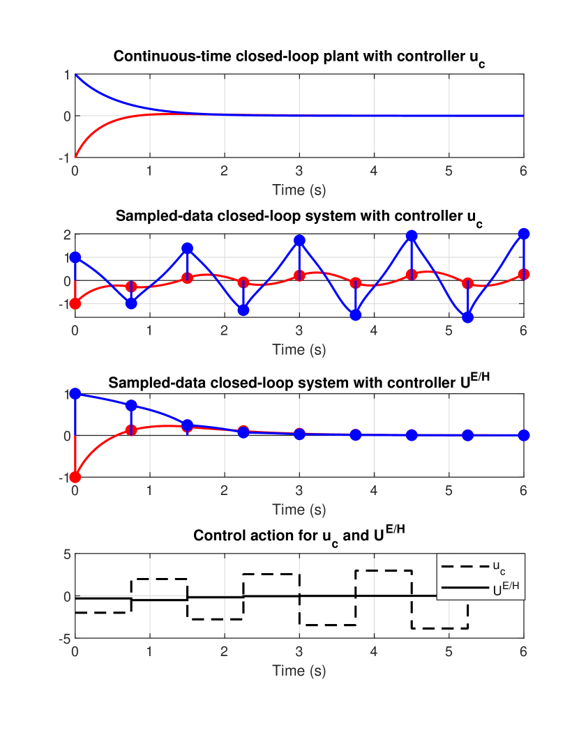
Figure 1: Evolution of the continuous/time closed/loop plant with $u_{c}=-2x_{2}$ compared with the evolution of the sampled/data system (8) in closed/loop with controllers $u_{c}$ and $U^{E/Heun}$ for a constant sampling period $T=0.75$. Blue: $x_{1}$. Red: $x_{2}$.

Figure 1 shows simulations from initial condition $x_{0}=[-1,1]^{T}$ for both sampled/data closed/loop models for a constant sampling period $T=0.75$. Note that for the used sampling instant sequence, emulation leads to unstable behaviour while the sampled/data evolution corresponding to the controller $U^{E/Heun}$ is stable and gets closer to the exact continuous/time solution $H^{e}$.

5 Conclusions

We presented mild consistency and regularity conditions on the plant and control laws that allow to establish novel relationships between the stability of a sampled/data system fed back with sampling-period-dependent control laws with the stability of the CT closed/loop plant obtained in the limit as the sampling period converges to zero. The given results extend previous ones under milder assumptions.

6 Proofs

6.1 Proof of Theorem 2.6

i). We will use the results in Vallarella and Haimovich [2019]. To do so define $G^{a}(x,u,T):=\bar{F}^{a}(x,T)$ and $G^{b}(x,u,T):=\bar{F}^{b}(x,T)$ for any $u$. We will now prove that the fact that $(\bar{F}^{a},\bar{F}^{b})$ is EPC implies that $(U,G^{a})$ is MSEC with $(U,G^{b})$ for any control law $U(x,T)$ according to [Vallarella and Haimovich, 2019, Definition 2.6].

Given $\mathcal{X}\subset\mathbb{R}^{n}$ compact, define $M:=\max\{|x|:x\in\mathcal{X}\}$. Let the EPC definition generate $K>0$, $T^{*}>0$ and $\rho\in\mathcal{K}_{\infty}$ such that

$$\left|\bar{F}^{a}(x,T)-\bar{F}^{b}(y,T)\right|\leq(1+KT)\left|x-y\right|+T\rho(T)\max\{|x|,|y|\}$$ (16)

for all $|x|,|y|\leq M$ and $T\in(0,T^{*})$. Define $\rho_{0}\in\mathcal{K}$ via $\rho_{0}:=M\rho$ and the constant (hence nondecreasing) function $\sigma:\mathbb{R}_{\geq 0}\to\mathbb{R}_{\geq 0}$, $\sigma\equiv K$. Then,

$$|\bar{F}^{a}(x,T)-\bar{F}^{b}(y,T)| =|G^{a}(x,u,T)-G^{b}(y,u,T)|$$

$$\leq T\rho_{0}(T)+(1+T\sigma(T))|x-y|$$

holds for all $u$ and $x,y\in\mathcal{X}$. In particular, for any control law $U$, if we substitute $u=U(x+e,T)$, it follows that

$$|\bar{G}^{a}_{U}(x,e,T)-\bar{G}^{b}_{U}(y,e,T)| :=|G^{a}(x,U(x+e,T),T)-G^{b}(y,U(y+e,T),T)|$$

$$\leq T\rho_{0}(T)+(1+T\sigma(T))|x-y|,$$

where we have employed the notation $\bar{G}^{a}_{U}(x,e,T)$ according to Vallarella and Haimovich [2019]. Therefore, the pair $(U,G^{a})$ is MSEC with $(U,G^{b})$ [Vallarella and Haimovich, 2019, Definition 2.6]. By [Vallarella and Haimovich, 2019, Theorem 3.1] this last fact is sufficient to ensure that if $x_{k+1}=\bar{G}^{a}_{U}(x_{k},e_{k},T_{k})$ is Semiglobally Practically Input-to-State Stable under nonuniform sampling (SP-ISS-VSR) as defined in [Vallarella and Haimovich, 2019, Definition 2.1] then so is $x_{k+1}=\bar{G}^{b}_{U}(x_{k},e_{k},T_{k})$ and viceversa. Note that the property SP-ISS-VSR [Vallarella and Haimovich, 2019, Definition 2.1] becomes SPS-VSR (Definition 2.5) in the absence of errors (inputs). Given that that $\bar{G}^{a}_{U}(x,e,T)=\bar{F}^{a}(x,T)$ and $\bar{G}^{b}_{U}(x,e,T)=\bar{F}^{b}(x,T)$ for all $e\in\mathbb{R}^{n}$ the result follows. $\circ$

ii). We will use the results in Vallarella et al. [2021]. To do so define $\bar{G}^{a}(x,e,T):=\bar{F}^{a}(x,T)$ and $\bar{G}^{b}(x,e,T):=\bar{F}^{b}(x,T)$ for any $e$. Note that if the pair $(\bar{F}^{a},\bar{F}^{b})$ is EPC then the pair $(\bar{G}^{a},\bar{G}^{b})$ is REPC as defined in [Vallarella et al., 2021, Definition 3.1]. Furthermore, the REPC property implies the REPMC property [Vallarella et al., 2021, Lemma 3.7], which is required to prove [Vallarella et al., 2021, Theorem 3.5].

The current proof is based on slight modifications of the proof of [Vallarella et al., 2021, Theorem 3.5]. We modify its first part to adapt it to the LES-VSR property under consideration:

Let $K_{a}\geq 1$ and $R_{a},T^{a},\lambda_{a}>0$, characterize the LES-VSR property of $x^{a}_{k+1}=\bar{G}^{a}(x^{a}_{k},e_{k},T_{k})$. Thus, for all $k\in\mathbb{N}_{0}$, $\{T_{i}\}\in\Phi(T^{a})$ and $|x_{0}|\leq R_{a}$ the solutions satisfy $|x^{a}_{k}|\leq K^{a}|x^{a}_{0}|e^{-\lambda_{a}\sum_{i=0}^{k-1}T_{i}}\leq K^{a}R_{a}=:R$. Let $\delta\in(0,1)$ and $\eta\in(0,\delta)$. Let $\mathcal{T}:=\frac{1}{\lambda_{a}}\ln\left({\frac{K_{a}}{\delta-\eta}}\right)$. Define $\mathcal{T}_{1}:=\mathcal{T}+1$ and let Vallarella et al. [2021, Lemma 3.4] generate $T^{L}=T^{L}(R,0,\mathcal{T}_{1},\eta)$. Define $\bar{T}<\min\{1,T^{a},T^{L}\}$. Consider sampling period sequences such that $\{T_{i}\}\in\Phi(\bar{T})$, and for every $k\in\mathbb{N}_{0}$ and $j\in\mathbb{N}$ define $s(k):=\sup\left\{r\in\mathbb{N}_{0}:r\geq k+1,\sum_{i=k}^{r-1}T_{i}\leq\mathcal{T}_{1}\right\}$ and $s^{j}(k):=\overbrace{s(\ldots s(s}^{j}(k)))$. From this expression the proof follows identically as in the proof of [Vallarella et al., 2021, Theorem 3.5] by performing the following minor changes: a) the quantity $E$ must be chosen as $E=0$, which implies that the error input sequence satisfies $e_{i}=0$ for all $i\in\mathbb{N}_{0}$, b) rename $M$ and $M_{a}$ by $R_{a}$ and $R$, respectively. Consequently, according to the proof of [Vallarella et al., 2021, Theorem 3.5], we obtain that the state evolution for the model $\bar{G}^{b}$ from the initial state $\xi$ satisfies the following condition

$$|x^{b}_{k}(\xi)| \leq K_{b}\exp{\left(-\lambda_{b}\sum_{i=0}^{k-1}T_{i}\right)}|\xi|$$ (17)

for all $k\in\mathbb{N}_{0}$, $|\xi|\leq R$ and $\{T_{i}\}\in\Phi(\bar{T})$, where $K_{b}:=(K_{a}+\eta)\exp{\left(\lambda_{b}\mathcal{T}_{1}\right)}$ $=(K_{a}+\eta)/\delta$ and $\lambda_{b}:=\ln({1/\delta})/\mathcal{T}_{1}$ and the result follows. $\circ$

iii). According to definition of SLES-VSR in Definition 2.4, this result is a direct consequence of the results in the previous items i) and ii). $\circ$

$\hfill\blacksquare$

6.2 Proof of Theorem 3.4.

Consider $M\geq 0$ given and $|x|,|y|\leq M$. Let the StC property of $(U,V)$ generate $T^{V}:=T^{V}(M)>0$ and $\tilde{\rho}\in\mathcal{K}_{\infty}$ and the StL property of $U$ generate $K_{U}:=K_{U}(M)>0$ and $T^{U}:=T^{U}(M)>0$. Thus $|U(x,T)|\leq K_{U}M$ for all $|x|\leq M$ and $T\in[0,T^{U})$. We can bound $|V(x,T)|=|V(x,T)-U(x,T)+U(x,T)|\leq|V(x,T)-U(x,T)|+|U(x,T)|\leq\tilde{\rho}(T^{V})M+K_{U}M=:E$. Let the StLC property of $F^{a}$ generate $K(M,E)>0$ and $T^{*}:=T^{*}(M,E)>0$. Define $\bar{K}:=K(1+K_{U})$ and $\rho\in\mathcal{K}_{\infty}$ via $\rho(s):=K\tilde{\rho}$. Define $T^{\star}:=\min\{T^{*},T^{V},T^{U}\}$ Then, for all $|x|,|y|\leq M$ and $T\in[0,T^{\star})$ we have

$$\left|F^{a}(x,U(x,T),T)-F^{a}(y,V(y,T),T)\right|$$

$$\leq(1+KT)|x-y|+KT|U(x,T)-V(y,T)|$$ (18)

$$=(1+KT)|x-y|+KT|U(x,T)-U(y,T)+U(y,T)-V(y,T)|$$

$$\leq(1+KT)|x-y|+KK_{U}T|x-y|+KT\tilde{\rho}(T)|y|$$ (19)

$$\leq(1+\bar{K}T)|x-y|+T\rho(T)\max\{|x|,|y|\}$$

In (18) and (19) we have used the facts that $F^{a}$ is StLC, $U$ is StL and $(U,V)$ is StC, respectively. $\hfill\blacksquare$

6.3 Proof of Theorem 3.5

To prove Theorem 3.5 we need Theorem 3.4 and the following Lemma 6.1 and Proposition 6.2, whose proofs are given at the end of this section. Lemma 6.1 establishes the relationship between CT stability properties of (2) and the DT model $H^{e}$, given by its samples; i.e. $H^{e}(x_{k},T_{k})$ is just the solution of (2) a time $T_{k}$ ahead from initial state $x_{k}$.

Lemma 6.1.

The CT closed/loop plant (2) is i) GAS $\Leftrightarrow$ $H^{e}$ is SPS-VSR. ii) LES $\Leftrightarrow$ $H^{e}$ is LES-VSR. iii) GALES $\Leftrightarrow$ $H^{e}$ is SLES-VSR. iv) GES $\Leftrightarrow$ $H^{e}$ is SES-VSR.

Proposition 6.2 shows that under Assumptions 2.2 and 2.3, the checkable mild sufficient conditions of StL for the control law $U$ and StC for the pair $(U,U_{c})$ ensure that the pair $(H^{e},\bar{F}^{e}_{U})$ is EPC. This establishes a correspondence between CT and sampled/data systems via Lemma 6.1.

Proposition 6.2.

Under the assumptions of Theorem 3.5, the pair $(H^{e},\bar{F}^{e}_{U})$ is EPC.

Note that asymptotic stability of (2) does not imply that $\bar{F}^{e}_{U}$ also exhibits asymptotic properties. Under the assumptions of Theorem 3.5, by Lemma 6.1, Proposition 6.2 and Theorem 2.6, the system (2) is GAS if and only if $\bar{F}^{e}_{U}$ is SPS-VSR (however GAS of (2) does not imply SS-VSR of $\bar{F}^{e}_{U}$ as one might intuitively think). Next we use Theorem 3.4, Lemma 6.1 and the following Lemma 6.3 to prove Proposition 6.2. Recall that $U_{c}(x,T):=u_{c}(x)$ for all $T$.

Lemma 6.3.

The following implications hold

1. Assumptions 2.2 and 2.3 $\Rightarrow$ $h$ is locally Lipschitz.

2. $h$ is locally Lipschitz $\Rightarrow$ $H^{e}$ is StLC. Moreover, for each $M\geq 0$ there exists $\bar{T}:=\bar{T}(M)$ such that for all $|x|\leq M$ and $T\in(0,\bar{T})$ we have $|H^{e}(x,T)|\leq 2M$.

3. $h$ is locally Lipschitz $\Rightarrow$ $(H^{e},\bar{F}^{E}_{U_{c}})$ is EPC.

4. Assumption 2.2 $\Rightarrow$ $F^{E}$ (Euler model) is StLC.

5. Assumption 2.3 $\Rightarrow$ $U_{c}$ is StL.

6. $F^{E}$ is StLC+ $U$ is StL+ $(U_{c},U)$ is StC $\Rightarrow$ $(\bar{F}_{U_{c}}^{E},\bar{F}^{E}_{U})$ is EPC.

7. Assumptions 2.2 and 2.3 +$U$ is StL $\Rightarrow$ $(\bar{F}^{E}_{U},\bar{F}^{e}_{U})$ is EPC.

Proof.

i) Consider $M\geq 0$ given. Define $L_{u_{c}}:=L_{u_{c}}(M)$ from Assumption 2.3, $L_{f}:=L_{f}(M,L_{u_{c}})$ from Assumption 2.2 and $L:=L_{f}(1+L_{u_{c}})$. For all $|x|,|y|\leq M$ we have

$$|h(x)-h(y)| =|f(x,u_{c}(x))-f(y,u_{c}(y))|\leq L_{f}(|x-y|+|u_{c}(x)-u_{c}(y)|)$$

$$\leq L_{f}(1+L_{u_{c}})|x-y|=L|x-y|.$$

$\circ$

ii) Consider $M\geq 0$ given. Let the locally Lipschitz property of $h$ generate $L_{h}:=L_{h}(M)>0$. Define $\bar{L}(M):=L_{h}(2M)>0$ and $\bar{T}(M):=\ln{(2)}/\bar{L}$. We claim that $|H^{e}(x,T)|\leq 2M$ for all $|x|\leq M$ and $T\in(0,\bar{T})$. For a contradiction, let $x$ and $T^{\prime}$ be such that $|x|\leq M$, $T^{\prime}\in(0,\bar{T})$ and $|H^{e}(x,T^{\prime})|>2M$. Define $\tau:=\inf\{T>0:|H^{e}(x,T)|>2M\}$. Then $|H^{e}(x,T)|\leq 2M$ for all $T\in(0,\tau]$ and $|H^{e}(x,\tau)|=2M$ by continuity, with $\tau<\bar{T}$. We have $|H^{e}(x,\tau)|\leq|x|+\int_{0}^{\tau}|h(H^{e}(x,s))|ds\leq M+\bar{L}\int_{0}^{\tau}|H^{e}(x,s)|ds.$ Using Gronwall inequality, then $|H^{e}(x,\tau)|\leq Me^{\bar{L}\tau}<Me^{\bar{L}\bar{T}}=2M$, reaching a contradiction. The claim is thus true. For all $|x|,|y|\leq M$ and $T\in(0,\bar{T})$ then

$$\left|H^{e}(x,T)-H^{e}(y,T)\right| \leq\left|x-y\right|+\int_{0}^{T}\left|h(H^{e}(x,s))-h(H^{e}(y,s))\right|ds$$

$$\leq\left|x-y\right|+\bar{L}\int_{0}^{T}\left|H^{e}(x,s)-H^{e}(y,s)\right|ds.$$

By Gronwall inequality then $|H^{e}(x,T)-H^{e}(y,T)|\leq e^{\bar{L}\bar{T}}\left|x-y\right|$, thus $H^{e}$ is StLC. $\circ$

iii) Consider $M>0$ given. Let the StLC property of $H^{e}$ generate $L_{H}:=L_{H}(2M)$ and $\bar{T}:=\bar{T}(M)$. From the claim in item ii), note that $|H^{e}(x,T)|\leq 2M$ for all $|x|\leq M$ and $T\in(0,\bar{T})$. Define $L_{h}:=L_{h}(2M)$ from the fact that $h$ is locally Lipschitz. Thus, for all $|x|,|y|\leq M$ and $T\in(0,\bar{T})$ we have

$$|H^{e}(x,T)-\bar{F}^{E}_{U_{c}}(y,T)|=\left|x+\int_{0}^{T}h(H^{e}(x,s))ds-y-Th(y)\right|$$

$$\leq\left|x-y\right|+L_{h}\int_{0}^{T}\left|H^{e}(x,s)-y\right|ds$$

$$\leq\left|x-y\right|+L_{h}\int_{0}^{T}\bigg{|}H^{e}(x,s)-y-\bar{F}^{E}_{U_{c}}(y,s)+\bar{F}^{E}_{U_{c}}(y,s)\bigg{|}ds$$

$$\leq\left|x-y\right|+L_{h}\int_{0}^{T}\left|H^{e}(x,s)-\bar{F}^{E}_{U_{c}}(y,s)\right|ds+L_{h}\int_{0}^{T}T\left|h(y)\right|ds$$

$$\leq\left|x-y\right|+L_{h}\int_{0}^{T}\left|H^{e}(x,s)-\bar{F}^{E}_{U_{c}}(y,s)\right|ds+L_{h}T^{2}\left|h(y)\right|.$$

By Gronwall inequality,

$$\left|H^{e}(x,T)-\bar{F}^{E}_{U_{c}}(y,s)\right| \leq\left(\left|x-y\right|+L_{h}T^{2}\left|h(y)\right|\right)e^{L_{h}T}$$

$$\leq|x-y|\left(1+\frac{e^{L_{h}T}-1}{T}\,T\right)+L_{h}^{2}T^{2}e^{L_{h}T}|y|$$

$$\leq\left(1+KT\right)\left|x-y\right|+\rho(T)T\left|y\right|$$

where $K:=(e^{L_{h}\bar{T}}-1)/\bar{T}=\left(L_{h}+\sum_{k=2}^{\infty}\frac{L_{h}^{k}\bar{T}^{k-1}}{k!}\right)$ and $\rho\in\mathcal{K}_{\infty}$ is defined as $\displaystyle\rho(s):=L_{h}^{2}e^{L_{h}\bar{T}}s$. $\circ$

iv) Consider $M,D\geq 0$ given, then $|F^{E}(x,u,T)-F^{E}(y,v,T)|\leq|x-y|+T|f(x,u)-f(y,v)|\leq|x-y|+TL(|x-y|+|u-v|)\leq(1+KT)|x-y|+KT|u-v|$ for all $|x|\leq M$, $|u|,|v|\leq D$, and $T\in[0,\infty)$ where we have used Assumption 2.2 and $K:=L$. $\circ$

v) By Assumption 2.3 $u_{c}(x)$ is locally Lipschitz. Given that it does not depend on $T$ the result is immediate. $\circ$

vi) Conditions of Theorem 3.4 hold, thus the result is immediate. $\circ$

vii) We will prove that Assumptions 2.1-2.3 (A2.1-2.3 in the following) and conditions i) and ii) of [Vallarella et al., 2021, Theorem 3.9] hold. Define $\bar{U}(x,e,T):=U(x,T)$ for each $q\in\mathbb{N}$ and all $e\in\mathbb{R}^{q}$. Thus, the closed-loop Euler and exact models result $\bar{F}^{E}_{U}(x,e,T):=\bar{F}^{E}(x,U(x,e,T),T)$ and $\bar{F}^{e}_{U}(x,e,T):=\bar{F}^{e}(x,U(x,e,T),T)$, respectively.

A2.1: It is a direct consequence of Assumption 2.2.

A2.2: Consider $M,C_{u}\geq 0$ given and $|x|\leq M$ and $|u|\leq C_{u}$. From Assumption 2.2 define $L:=L(M,C_{u})$ and function $C_{f}(r,s):=L(r+s)$, then for all $|x|\leq M$ and $|u|\leq C_{u}$ $|f(x,u)|=|f(x,u)-f(0,0)|\leq L(|x|+|u|)\leq L(M+C_{u}):=C_{f}(M,C_{u})$.

A2.3: Consider $M,E\geq 0$ given. Define $L:=L(M)$ from Assumption 2.3 and $K:=K(M)$, $T^{*}(M)$ from the fact that $U$ is StL. Define $T_{u}(M,E):=\min\{1,T^{*}(M)\}$ and for all $|x|\leq M$, $|e|\leq E$ and $T\in[0,T_{u})$, we have $|\bar{U}(x,e,T)|\leq|U(x,T)-U(0,T)|+|U(0,T)|\leq K|x|\leq KM=:C_{u}(M,E)$.

Condition i): The result is immediate, since we have that $f(0,\bar{U}(0,e,T))=f(0,U(0,T))=f(0,0)=0$.

Condition ii): From A2.3, and $T\in(0,T_{u})$ we have that $|\bar{U}(x,e,T)|\leq C_{u}(M,E)$. Define $L:=L(M,C_{u}(M,E))$ from Assumption 2.2. For all $|x^{a}|,|x^{b}|\leq M$, $|e|\leq E$ and $T\in(0,T_{u})$ we have $|f(x^{a},\bar{U}(x^{a},e,T))-f(x^{b},\bar{U}(x^{b},e,T))|\leq L(|x^{a}-x^{b}|+|\bar{U}(x^{a},e,T)-\bar{U}(x^{b},e,T)|)\leq L(|x^{a}-x^{b}|+K|x^{a}-x^{b}|)\leq L(1+K)|x^{a}-x^{b}|$. Thus, by [Vallarella et al., 2021, Theorem 3.9] the pair $(\bar{F}^{RK}_{U},\bar{F}^{e}_{U})$ is REPC. By assuming that no errors affect the control input, i.e. $e=0$, REPC coincide with the EPC property and therefore $(\bar{F}^{RK}_{U},\bar{F}^{e}_{U})$ is EPC for any explicit Runge-Kutta (RK) model. Given that the Euler model is the simplest RK model, $(\bar{F}^{E}_{U},\bar{F}^{e}_{U})$ is EPC and the result follows. $\circ$$\hfill\blacksquare$

Proof of Lemma 6.1.

Proof of item i)

$\Longrightarrow$) Let the GAS property of (2) generate $\beta\in\mathcal{KL}$ from i) of Definition 2.1. We have $|x(t)|\leq\beta(|x_{0}|,t),\medspace\forall t\geq 0$. Then,

$$|x_{k}|\leq\beta\left(|x_{0}|,\sum_{i=0}^{k-1}T_{k}\right)$$ (20)

for all $k\in\mathbb{N}_{0}$, $\{T_{i}\}\in\Phi(\infty)$ and $x_{0}\in\mathbb{R}^{n}$. Thus, $H^{e}$ is SS-VSR with $T^{*}:=\infty$, and hence SPS-VSR by the fact that SS-VSR implies SPS-VSR.

$\Longleftarrow$) Let the SPS-VSR property of $H^{e}$ generate $\beta\in\mathcal{KL}$ and $T^{*}:=T^{*}(M,R)$ for every $M,R>0$ such that the bound $|x_{k}|\leq\beta\left(|x_{0}|,\sum_{i=0}^{k-1}T_{k}\right)+R$ holds for all $k\in\mathbb{N}_{0}$, $\{T_{i}\}\in\Phi(T^{*})$ and $|x_{0}|\leq M$. We next establish GAS with function $\bar{\beta}:=2\beta\in\mathcal{KL}$.

Consider $x_{0}\in\mathbb{R}^{n}$ and $t\geq 0$ given. Define $M:=|x_{0}|$ and the constants $R\in(0,1)$ such that $R\leq\beta(M,t)$ and $N\in\mathbb{N}$ such that $N\geq\frac{2t}{T^{*}(M,R)}$. Define the constant sampling period sequence as $T_{k}\equiv\frac{t}{N}\leq T^{*}/2$. Note that $\sum_{i=0}^{N-1}T_{i}=t$ and $x(t)=x_{N}$. Thus,

$$|x(t)|\leq\beta\left(|x_{0}|,\sum_{i=0}^{N-1}T_{i}\right)+R=\beta\left(|x_{0}|,t\right)+R\leq\bar{\beta}\left(|x_{0}|,t\right).$$ (21)

Given that (21) holds for any given $x_{0}\in\mathbb{R}^{n}$ and $t\geq 0$ the result follows. $\circ$

Proof of item ii)

$\Longrightarrow$) Let the LES property of (2) generate $K\geq 1$ and $R,\lambda>0$. We have $|x(t)|\leq K|x_{0}|e^{-\lambda t},\medspace\forall t\geq 0$. Then, $|x_{k}|\leq K|x_{0}|e^{-\lambda\sum_{i=0}^{k-1}T_{i}}$ for all $k\in\mathbb{N}_{0}$, $\{T_{i}\}\in\Phi(\infty)$ and $|x_{0}|\leq R$ and thus, $H^{e}$ is LES-VSR.

$\Longleftarrow$) Let the LES-VSR property of $H^{e}$ generate $K\geq 1$ and $R,T^{*},\lambda>0$ and consider $|x_{0}|\leq R$ given such that the bound $|x_{k}|\leq K|x_{0}|e^{-\lambda\sum_{i=0}^{k-1}T_{i}}$ holds for all $k\in\mathbb{N}_{0}$, $\{T_{i}\}\in\Phi(T^{*})$ and $|x_{0}|\leq R$. Consider a sampling period sequence such that $T_{k}\equiv\frac{aT^{*}}{2}$ with $a\in(0,1]$ for all $k\in\mathbb{N}_{0}$. Define $t(k):=\frac{aT^{*}}{2}k$. Thus, for the given initial condition $x_{0}$ we have $|x_{k}|\leq K|x_{0}|\exp\left(-\lambda t(k)\right)$ for all $k\in\mathbb{N}_{0}$. Given that, irrespectibly of $x_{0}\in\mathbb{R}^{n}$, the previous bound holds for any $a\in(0,1]$ it also holds for any $t\in\mathbb{R}_{\geq 0}$ and the result follows. $\circ$

Proof of item iii) The result follows directly from the proofs of items i) and ii) and the GALES definition. $\circ$

Proof of item iv) $\Longrightarrow$) Let the GES property of (2) generate $\lambda>0$ and $K\geq 1$. We have $|x(t)|\leq K|x_{0}|\exp(-\lambda t),\medspace\forall t\geq 0$. Then

$$|x_{k}|\leq K|x_{0}|\exp\left(-\lambda\sum_{i=0}^{k-1}T_{k}\right)$$ (22)

for all $k\in\mathbb{N}_{0}$, $\{T_{i}\}\in\Phi(\infty)$ and $x_{0}\in\mathbb{R}^{n}$. Thus, $H^{e}$ is SES-VSR with $T^{*}:=\infty$.

$\Longleftarrow$) Consider that $H^{e}$ is SES-VSR. Consider $x_{0}\in\mathbb{R}^{n}$ given. Define $M:=|x_{0}|$, and let the SES-VSR property of $H^{e}$ generate $\lambda>0$, $K\geq 1$ and $T^{*}:=T^{*}(M)$ such that the bound (22) holds for all $k\in\mathbb{N}_{0}$, $\{T_{i}\}\in\Phi(T^{*})$ and the given $x_{0}$. Consider a sampling period sequence such that $T_{k}\equiv\frac{aT^{*}}{2}$ with $a\in(0,1]$ for all $k\in\mathbb{N}_{0}$. Define $t(k):=\frac{aT^{*}}{2}k$. Thus, for the given initial condition $x_{0}$ we have $|x_{k}|\leq K|x_{0}|\exp\left(-\lambda t(k)\right)$ for all $k\in\mathbb{N}_{0}$. Given that, irrespectibly of $x_{0}\in\mathbb{R}^{n}$, this last bound holds for any $a\in(0,1]$ it also holds for any $t\in\mathbb{R}_{\geq 0}$ and the result follows. $\circ$

$\hfill\blacksquare$

Proof of Proposition 6.2.

By the implications in Lemma 6.3, the pairs $(H^{e},\bar{F}^{E}_{U_{c}})$, $(\bar{F}^{E}_{U_{c}},\bar{F}^{E}_{U})$ and $(\bar{F}^{E}_{U},\bar{F}^{e}_{U})$ are EPC. By the transitivity of the EPC property $(H^{e},\bar{F}^{e}_{U})$ is EPC. $\hfill\blacksquare$

Proof of Theorem 3.5.

Conditions of Proposition 6.2 imply that $(H^{e},\bar{F}^{e}_{U})$ is EPC. Consider that $\bar{F}^{e}_{U}$ or $H^{e}$ fulfills the SES-VSR, LES-VSR or SLES-VSR properties. By Theorem 2.6, $H^{e}$ or $\bar{F}^{e}_{U}$ fulfills the same properties, respectively. By the implications of Lemma 6.1 the result follows. $\hfill\blacksquare$

References

• Beikzadeh et al. [2018] Beikzadeh, H., Liu, G., Marquez, H.J., 2018. Robust sensitive fault detection and estimation for single-rate and multirate nonlinear sampled-data systems. Systems & Control Letters 119, 71–80.
• Di Ferdinando and Pepe [2019] Di Ferdinando, M., Pepe, P., 2019. Sampled-data emulation of dynamic output feedback controllers for nonlinear time-delay systems. Automatica 99, 120–131.
• Di Ferdinando et al. [2021] Di Ferdinando, M., Pepe, P., Fridman, E., 2021. Exponential input-to-state stability of globally lipschitz time-delay systems under sampled-data noisy output feedback and actuation disturbances. International Journal of Control 94, 1682–1692.
• Grüne et al. [2008] Grüne, L., Worthmann, K., Nešić, D., 2008. Continuous-time controller redesign for digital implementation: A trajectory based approach. Automatica 44, 225–232.
• Hetel et al. [2017] Hetel, L., Fiter, C., Omran, H., Seuret, A., Fridman, E., Richard, J.P., Niculescu, S.I., 2017. Recent developments on the stability of systems with aperiodic sampling: An overview. Automatica 76, 309–335.
• Khalil [2002] Khalil, H., 2002. Nonlinear Systems. Pearson Education, Prentice Hall.
• Li and Zhao [2018] Li, Z., Zhao, J., 2018. Output feedback stabilization for a general class of nonlinear systems via sampled-data control. International Journal of Robust and Nonlinear Control 28, 2853–2867.
• Lin [2020] Lin, W., 2020. When is a nonlinear system semiglobally asymptotically stabilizable by digital feedback? IEEE Transactions on Automatic Control 65, 4584–4599.
• Lin and Sun [2021] Lin, W., Sun, J., 2021. New results and examples in semiglobal asymptotic stabilization of nonaffine systems by sampled-data output feedback. Systems & Control Letters 148, 104850.
• Lin and Wei [2018] Lin, W., Wei, W., 2018. Semiglobal asymptotic stabilization of lower triangular systems by digital output feedback. IEEE Transactions on Automatic Control 64, 2135–2141.
• Liu et al. [2008] Liu, X., Marquez, H.J., Lin, Y., 2008. Input-to-state stabilization for nonlinear dual-rate sampled-data systems via approximate discrete-time model. Automatica. 44, 3157–3161.
• Monaco and Normand-Cyrot [2007] Monaco, S., Normand-Cyrot, D., 2007. Advanced tools for nonlinear sampled-data systems’ analysis and control. European Journal of Control 13, 221–241.
• Nešić et al. [1999] Nešić, D., A. R. Teel, Kokotović, P.V., 1999. Sufficient conditions for stabilization of sampled-data nonlinear systems via discrete-time approximations. Systems & Control Letters. 38, 259–270.
• Nešić et al. [2009a] Nešić, D., Loría, A., Panteley, E., Teel, A.R., 2009a. On stability of sets for sampled-data nonlinear inclusions via their approximate discrete-time models and summability criteria. SIAM Journal on Control and Optimization. 48, 1888–1913.
• Nešić and Teel [2004] Nešić, D., Teel, A.R., 2004. A framework for stabilization of nonlinear sampled-data systems based on their approximate discrete-time models. IEEE Transactions on Automatic Control. 49, 1103–1122.
• Nešić et al. [2009b] Nešić, D., Teel, A.R., Carnevale, D., 2009b. Explicit computation of the sampling period in emulation of controllers for nonlinear sampled-data systems. IEEE Transactions on Automatic Control 54, 619–624.
• Nešić and Grüne [2005] Nešić, D., Grüne, L., 2005. Lyapunov-based continuous-time nonlinear controller redesign for sampled-data implementation. Automatica 41, 1143–1156.
• Noroozi et al. [2018] Noroozi, N., Mousavi, S.H., Marquez, H.J., 2018. Integral versions of input-to-state stability for dual-rate nonlinear sampled-data systems. Systems & Control Letters 117, 11–17.
• Omran et al. [2016] Omran, H., Hetel, L., Petreczky, M., Richard, J.P., Lamnabhi-Lagarrigue, F., 2016. Stability analysis of some classes of input-affine nonlinear systems with aperiodic sampled-data control. Automatica 70, 266–274.
• Postoyan et al. [2008] Postoyan, R., Ahmed-Ali, T., Burlion, L., Lamnabhi-Lagarrigue, F., 2008. On the Lyapunov-based adaptive control redesign for a class of nonlinear sampled-data systems. Automatica 44, 2099–2107.
• Proskurnikov [2020] Proskurnikov, A.V., 2020. Does sample-time emulation preserve exponential stability?, in: Proceedings of the 23rd International Conference on Hybrid Systems: Computation and Control, pp. 1–8.
• Stuart and Humphries [1996] Stuart, A., Humphries, A., 1996. Dynamical Systems and numerical analysis. Cambridge University Press: NY.
• Üstüntürk [2012] Üstüntürk, A., 2012. Output feedback stabilization of nonlinear dual-rate sampled-data systems via an approximate discrete-time model. Automatica 48, 1796–1802.
• Üstüntürk and Kocaoğlan [2013] Üstüntürk, A., Kocaoğlan, E., 2013. Backstepping designs for the stabilisation of nonlinear sampled-data systems via approximate discrete-time model. International Journal of Control 86, 893–911.
• Vallarella et al. [2021] Vallarella, A.J., Cardone, P., Haimovich, H., 2021. Semiglobal exponential input-to-state stability of sampled-data systems based on approximate discrete-time models. Automatica 131, 109742.
• Vallarella and Haimovich [2018] Vallarella, A.J., Haimovich, H., 2018. Characterization of semiglobal stability properties for discrete-time models of non-uniformly sampled nonlinear systems. Systems & Control Letters 122, 60–66.
• Vallarella and Haimovich [2019] Vallarella, A.J., Haimovich, H., 2019. State measurement error-to-state stability results based on approximate discrete-time models. IEEE Transactions on Automatic Control. 64, 3308–3315.
Refer to caption