Privacy Leakage of Adversarial Training Models in Federated Learning Systems

Abstract

Adversarial Training (AT) is crucial for obtaining deep neural networks that are robust to adversarial attacks, yet recent works found that it could also make models more vulnerable to privacy attacks. In this work, we further reveal this unsettling property of AT by designing a novel privacy attack that is practically applicable to the privacy-sensitive Federated Learning (FL) systems. Using our method, the attacker can exploit AT models in the FL system to accurately reconstruct users’ private training images even when the training batch size is large. Code is available at https://github.com/zjysteven/PrivayAttack_AT_FL.

1 Introduction

Deep Neural Networks (DNNs) suffer from the notorious adversarial perturbations [17]: These imperceptible noises could easily fool DNNs to yield wildly wrong and malicious decisions (e.g., misclassification with high confidence). Adversarial Training (AT) [9] has been one of the most effective techniques that mitigate such vulnerability, which withstands adaptive attacks [18] and leads to the highest empirical adversarial robustness to date [1]. It is without doubt that AT is crucial for building robust intelligent systems.

Despite the desired robustness, recent works [16, 12] revealed an unexpected and alarming property of AT: It can make models more likely to leak the data privacy than the ones that undergoes vanilla training (i.e., using the original clean images instead of online-generated adversarial examples). Specifically, Song et al. [16] found that AT makes it easier for membership inference attack [14] to succeed, which aims to identify whether a certain sample was used during the training. In another work [12], it is shown that model inversion attack [4] is tractable on AT models, with which the attacker can generate images that visually resemble the actual training samples. In all, both papers indicated that AT models exhibit a robustness-privacy trade-off.

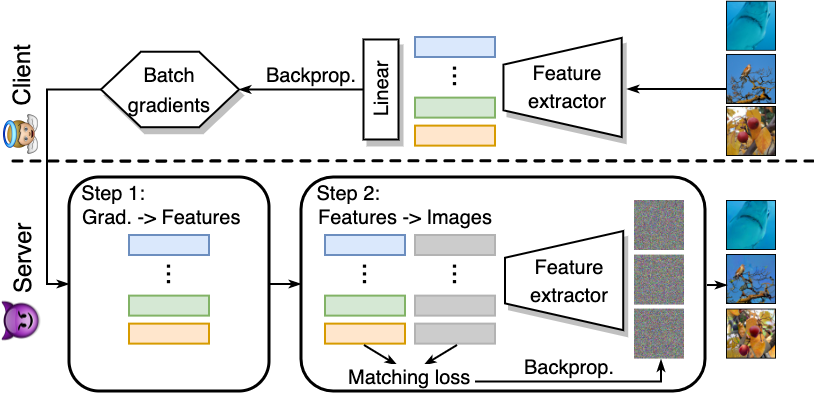
Figure 1: An overview of the proposed privacy attack against FL systems to “steal” the client’s training images. We formulate a novel two-step procedure: 1) Feature restoration from gradients (Sec. 4.2) and 2) Image reconstruction from features (Sec. 4.3). Zoom in and also refer Fig. 5 to see image reconstruction quality.

In this work, we pursue this line of inquiry and further demonstrate such trade-off by presenting a novel privacy attack that exploits AT models. Our attack is practically applicable to Federated Learning (FL) systems [11]. The goal is to compromise the privacy of FL clients by reconstructing their own training images (which may contain private information) based on the weight gradients that are communicated between the clients and the central server.

Different from previous approaches that directly invert gradients to reconstruct images [24, 5, 19], our attack methodology forms a unique two-step procedure, where we first restore the features (i.e., the outputs of the penultimate layer) from the gradients, and then reconstruct the inputs using the recovered features as supervision (see Fig. 1 for illustration). The key insight behind our method is that while the gradients of the samples within a batch are fused together and prohibit accurate reconstruction of each individual input, the features are less coupled and (once restored) can provide more precise information for the reconstruction than the batch-averaged gradients. Upon the general framework, the proposed attack leverages AT models which enable the success execution of both attack steps.

We conduct extensive experiments using high-resolution images from ImageNet [2] to demonstrate how our privacy attack can work with AT models to compromise the privacy of FL clients. Specifically, we are able to accurately reconstruct the clients’ training images at a large batch size (e.g., 256), something that is not achieved by previous methods with vanilla models [24, 5, 19]. The results suggest that AT poses a risk to the expected-to-be-secure FL systems.

2 Related Work

Privacy risks of AT models. As discussed earlier, a few prior works [16, 12] also identified that AT could make models more vulnerable to privacy attacks. In comparison, our work focuses on a considerably more strict and challenging criterion of privacy leakage: We consider exact reconstruction of the training images owned by the victims, a scenario which we believe poses more severe risks than the attacks that synthesize human-recognizable images [12] or infer the membership of data samples [16]. Besides, we put ourselves in the realistic, privacy-sensitive FL setting, to which our attack is practically applicable.

Privacy attacks against FL systems. There has been a line of research trying to expose the privacy vulnerability of the FL systems. Zhu et al. [24] developed the seminal DLG attack which reconstructs input images by matching the gradients computed using the reconstructed ones and the real ones. Geiping et al. [5] made improvements by using a better matching loss function and optimizer. They achieved near-perfect recovery quality when the gradients are computed using a single image (i.e., the batch size is 1). More recently, Yin et al. [19] further incorporated advanced image priors as regularization to enhance the recover quality.

All these works, however, can only unveil clear visual information under a small batch size (e.g., when the batch includes only a single or a few images), while a large batch size (e.g., 128 or 256) is often required for effective and efficient training of DNNs [6, 8]. As a result, whether the privacy can really be compromised in realistic settings (i.e., with large batch size) remains unclear. In this paper, we show that the privacy of FL clients is indeed at risk if they are performing AT, as the attacker can leverage our attack and exploit AT models to achieve accurate reconstruction of users’ images even at a batch size of 256.

Inverting features to reconstruct images. Inverting the features has been studied as a way to understand/interpret what DNN models learn [10, 3]. In particular, Engstrom et al. [3] discovered that AT models are more “invertible” than vanilla models, as the reconstructed images from AT models’ features look much more plausible. However, their focus is on the interpretability perspective. In our work, we take the security perspective and demonstrate how the good “invertibility” of AT models can unexpectedly/undesirably enable a privacy attack.

3 Problem Setting

We first formulate the problem setting and define the threat model before delving into our proposed attack. In a FL system, in each step the client will receive a copy of the global model from the central server and perform local training. Here, following prior works [24, 5, 19], we focus on the case of single-step local training. Concretely, considering an image classification task, the gradients of loss w.r.t. the model parameters are computed as follows during the local training:

$$\Delta_{\theta}\coloneqq\frac{1}{N}\sum_{i=1}^{N}\nabla_{\theta}\mathcal{L}(f_{\theta}(\bm{x}_{i}),y_{i}),$$ (1)

where $f_{\theta}(\cdot)$ is the mapping function of the DNN model parameterized by $\theta$, $N$ is the batch size, $\bm{x}_{i}$ is $i$-th input image of the batch, $y_{i}$ is the corresponding groundtruth label, $\mathcal{L}(\cdot,\cdot)$ computes the cross-entropy loss, and $\Delta_{\theta}$ is a simplified notion for the batch-averaged gradients. Note, if the client is performing AT, the input $\bm{x}_{i}$ will be the adversarial example instead of the original clean sample.

After the local training, the server will collect the gradients $\Delta_{\theta}$ from the clients and aggregate the updates into the current global model $f_{\theta}(\cdot)$. Here, we assume that the server is malicious or has been compromised by the attacker. Therefore, the attacker can access the model $f_{\theta}(\cdot)$ and the gradients $\Delta_{\theta}$. Similar to [5], we do not pose any further assumptions beyond this point which may allow the attacker to better exploit the vulnerability, e.g., we do not assume that the attacker can modify the model architecture or send fake, malicious global parameters to the clients. The attack goal is then to reconstruct the input images $\bm{x}_{i}$ that are used during the last local training step, given the available information $f_{\theta}(\cdot)$ and $\Delta_{\theta}$.

4 Methodology

4.1 Overview

To better motivate and describe our proposed methodology, we first give a brief overview of existing methods [24, 5, 19] and discuss their shortcomings. Essentially, previous works all solve the following optimization problem:

$$\operatorname*{arg\,min}_{\bm{z}}\mathcal{L}_{\text{grad}}\left(\frac{1}{N}\sum_{i=1}^{N}\nabla_{\theta}\mathcal{L}(f_{\theta}(\bm{z}_{i}),\hat{y}_{i}),\Delta_{\theta}\right)+\mathcal{R}(\bm{z}).$$ (2)

Specifically, the optimization variable here is a randomly-initialized batch of inputs $\bm{z}$. The first term in Eq. 2 enforces the gradients of loss computed using $\bm{z}$ to match the ground-truth gradients $\Delta_{\theta}$ according to a certain distance metric $\mathcal{L}_{\text{grad}}(\cdot,\cdot)$ (e.g., cosine distance is used in [5] and $\ell_{2}$ distance is used in [24] and [19]). Note, an estimation of the ground-truth labels $\hat{y}_{i}$ is used here to compute the loss [23, 5, 19]. The underlying idea of the first term is that the synthesized images $\bm{z}$ will resemble the original inputs if the gradients computed on them are similar. Meanwhile, to encourage the generation of realistic and natural images, the second term in Eq. 2 incorporates image priors $\mathcal{R}(\cdot)$ as regularization (e.g., the Total Variation loss [10] and the Group Consistency loss [19]).

While the idea of Eq. 2 is natural and straightforward, one can identify an obvious limitation. Note from Eq. 1 that the gradients contributed by each individual sample, i.e., $\nabla_{\theta}\mathcal{L}(f_{\theta}(x_{i}),y_{i})$, are fused together in the batch-averaged gradients $\Delta_{\theta}$. Therefore, $\Delta_{\theta}$ does not provide precise supervision for each individual image especially under a large batch size, making it much difficult to achieve accurate reconstruction (in a similar sense to how exactly knowing the value of $a$ and $b$ is hard given the value of $a+b$). As a result, Eq. 2 only works well when the batch size is extremely small (e.g., when the batch has only a single or a few samples). When the batch size is large, the restored images lack clear visual details and do not resemble the real images anymore [5, 19].

To mitigate this problem, we propose a unique two-step attack procedure. In the first step, we decouple the fused information of each individual image by restoring their features from the gradients which are less coupled. Here, we define the feature vector of a sample as the output of the penultimate layer when that sample is passed through the DNN model. Once we restore the feature vectors, each corresponding to one input image, we can use them as more accurate supervision to reconstruct the images. Next, we will explain each of the two steps in detail and discuss how AT models kick in and benefit the attack.

4.2 Feature restoration from gradients

We first introduce some notions to facilitate the description. A DNN model $f(\cdot)$ deployed for image classification tasks can always be decomposed as $f(\cdot)=h(r(\cdot))$, where $r(\cdot)$ typically comprises convolutional layers and extracts high-level representations/features of the inputs, and $h(\cdot)$ is the linear layer that performs classification on top of the features and outputs activation scores for each class (i.e., logits). For simplicity, we denote the feature of an input $\bm{x}$ as $\bm{r}$, i.e., $\bm{r}\coloneqq r(\bm{x})$. Note that $\bm{r}\in\mathbb{R}^{D}$ is a $D$-dimensional column vector.

Our key insight here is that the features can be restored from the gradients w.r.t. the linear layer’s weights, which are directly accessible to the attacker. To see this, let us first delve into the computation of the weight gradients of $h(\cdot)$. Denote the linear layer’s weight matrix as $\bm{W}\in\mathbb{R}^{D\times K}$, wherein the $k$-th column $\bm{W}_{k}\in\mathbb{R}^{D}$ is a weight vector corresponding to the $k$-th class, and $K$ is the total number of classes. Then, the class activations/logits are $\bm{a}=\bm{W}^{\top}\bm{r}$, and the class probabilities are $\bm{p}=\text{softmax}(\bm{a})$, where the probability on $k$-th class $\bm{p}_{k}$ is $\frac{e^{\bm{a}_{k}}}{\sum_{j=1}^{K}e^{\bm{a}_{j}}}$. Here, $\bm{a}_{k}=\bm{W}_{:,k}^{\top}\bm{r}$ is the $k$-th element of the vector $\bm{a}$, with $\bm{W}_{:,k}$ being the $k$-th column of $\bm{W}$. Finally, the cross-entropy loss computed on an input pair $(\bm{x},y)$ is $l=-\log\bm{p}_{y}$. Accordingly, one can derive the gradients of loss w.r.t. each weight vector $\bm{W}_{:,k}$ in the linear layer:

$$\frac{\partial l}{\partial\bm{W}_{:,k}} =\frac{\partial l}{\partial\bm{p}_{y}}\cdot\sum_{j=1}^{K}\frac{\partial\bm{p}_{y}}{\partial\bm{a}_{j}}\cdot\frac{\partial\bm{a}_{j}}{\bm{W}_{:,k}}$$

$$=\begin{cases}-(1-\bm{p}_{y})\bm{r},&k=y\\ ~{}~{}~{}~{}~{}~{}~{}~{}~{}~{}~{}~{}~{}\bm{p}_{k}\bm{r},&k\neq y\end{cases}.$$ (3)

Based on the derivation in Eq. 3, we now discuss how one can restore the features from the batch-averaged gradients w.r.t. the linear layer’s weights. We consider a batch of $N$ inputs $\bm{x}_{i}$, each with a corresponding feature vector $\bm{r}_{i}$. Note, following [5, 19], here we assume that there are no samples sharing the same label within the batch. This assumption generally holds for the randomly constructed batch when the size $N$ is (much) smaller than the number of classes $K$ (e.g., on ImageNet $K=1000$ while $N$ typically takes 256 [6]). Then, suppose that we want to restore the feature vector $\bm{r}_{i}$ whose corresponding label is $y_{i}$, we can directly take the gradients w.r.t. the weight vector $\bm{W}_{:,y_{i}}$:

$$\hat{\bm{r}}_{i} \coloneqq\Delta_{\bm{W}_{:,y_{i}}}=\frac{1}{N}\sum_{j=1}^{N}\frac{\partial l_{j}}{\partial\bm{W}_{:,y_{i}}}$$

$$\propto-(1-\bm{p}_{i,y_{i}})\bm{r}_{i}+\sum_{j=1,j\neq i}^{N}\bm{p}_{j,y_{i}}\bm{r}_{j}$$

$$\approx-(1-\bm{p}_{i,y_{i}})\bm{r}_{i}.$$ (4)

Here, we denote the restored feature vector as $\hat{\bm{r}}_{i}$. $l_{j}$ is the loss computed on the $j$-th image, and $\bm{p}_{i,y_{i}}$ represents the probability of the $i$-th sample belonging to class $y_{i}$.

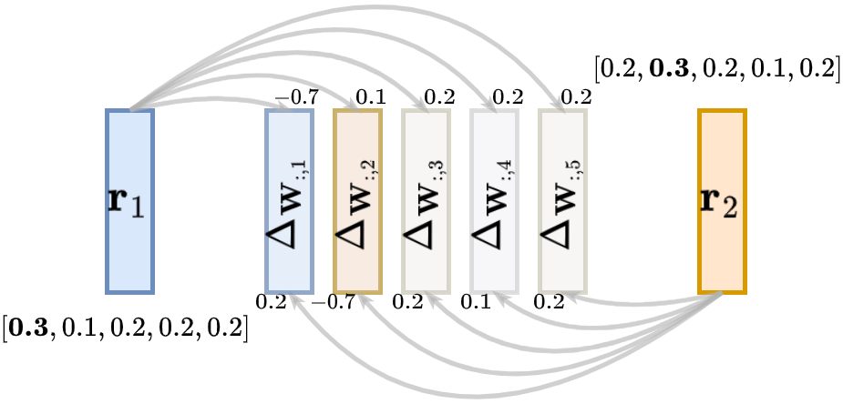
Figure 2: A toy example showcasing how the features can be restored from the linear layer’s weight gradients on an AT model. Here we suppose the batch size $N=2$ and the number of classes $K=5$. Without loss of generality, assume $\bm{r}_{1}$ and $\bm{r}_{2}$ have label $1$ and $2$, respectively. The numbers in the brackets are the softmax probabilities. Adversarial examples result in small $\bm{p}_{1,1}$ and $\bm{p}_{2,2}$. According to Eq. 4, $\Delta_{\bm{W}_{:,1}}\propto-(1-0.3)\bm{r}_{1}+0.2\bm{r}_{2}$. The attacker can take $\Delta_{\bm{W}_{:,1}}$ as the restored feature $\hat{\bm{r}}_{1}$.

Essentially, Eq. 4 indicates that the restored feature $\hat{\bm{r}}_{i}$ is approximately proportional to the true feature $\bm{r}_{i}$. The approximation in the last row of Eq. 4 holds because the probabilities assigned to the wrong class $\bm{p}_{j,y_{i}}$ (recall that $y_{j}\neq y_{i}$ when $j\neq i$) are becoming smaller and smaller as the training proceeds, therefore they may contribute much less to the summation than $-(1-\bm{p}_{i,y_{i}})\bm{r}_{i}$, especially if $\bm{p}_{i,y_{i}}$ is not too large. In fact, this is exactly the case for an AT model. During each iteration, AT uses adversarial examples as inputs, which are generated by maximizing the cross-entropy loss. Equivalently, adversarial examples minimize the probability assigned to the ground-truth class, i.e., $\bm{p}_{i,y_{i}}$. As a result, AT models can lead to a more tight approximation of Eq. 4 and better restoration of the features. We present a toy example of the feature restoration process in Fig. 2. Note, although in the case of AT the attacker is actually reconstructing the adversarial example, the privacy can still be compromised because the adversarial image is visually very similar to the clean image since their distance is bounded by a small value.

We finally discuss how to recover the batch labels $y_{i}$, which is necessary for knowing which columns of the gradient matrix of $\bm{W}$ should be taken for feature restoration. Here we adopt the common practice of existing works [23, 5, 19], which is to look at the sign of the gradient elements of $\bm{W}$. For the ease of illustration, without loss of generality, assume that the batch of $N$ samples are with the labels $1,2,...,N$, i.e., the $k$-th sample is from the $k$-th class. Then according to Eq. 4, the gradients w.r.t. the $k$-th column of $\bm{W}$ are:

$$\frac{1}{N}\sum_{j=1}^{N}\frac{\partial l_{j}}{\partial\bm{W}_{:,k}}\propto$$

$$~{}~{}~{}~{}~{}~{}\begin{cases}-(1-\bm{p}_{k,k})\bm{r}_{k}+\sum_{j=1,j\neq k}^{N}\bm{p}_{j,k}\bm{r}_{j},&~{}1\leq k\leq N\\ \sum_{j=1}^{N}\bm{p}_{j,k}\bm{r}_{j},&N<k\leq K\end{cases}.$$ (5)

Note that modern DNN architectures (e.g., ResNet [6] and VGG [15]) typically use ReLU as the activation function, which makes the elements of the feature vector $\bm{r}$ always non-negative. With this in mind, the takeaway of Eq. 5 is that in the gradient matrix of $\bm{W}$, only the columns that correspond to the appeared labels may have negative elements, while the other columns will have all positive values. Therefore, we can determine the batch labels by checking the sign of the smallest value of each column. If the smallest value of $k$-th column is positive, then $k$ is very unlikely to be one of the batch labels. In practice, one can pick the top-$N$ columns that have the smallest elements, and take their indices as the batch labels.

4.3 Image reconstruction from features

Once we obtain the restored feature $\hat{\bm{r}}_{i}$, the attacker can reconstruct each input image by solving the following optimization objective:

$$\operatorname*{arg\,min}_{\bm{z}_{i}}\mathcal{L}_{\text{feat}}\left(r_{\theta}(\bm{z}_{i}),\hat{\bm{r}}_{i}\right)+\mathcal{R}(\bm{z}_{i}).$$ (6)

The idea here is to optimize the input $\bm{z}_{i}$ such that its feature $r_{\theta}(\bm{z}_{i})$ is close to the restored feature $\hat{\bm{r}}_{i}$ (which in turn is similar to the ground-truth feature $\bm{r}_{i}$) according to a certain metric $\mathcal{L}_{\text{feat}}(\cdot,\cdot)$. Here we opt to use the scale-invariant cosine distance as $\mathcal{L}_{\text{feat}}$ since $\hat{\bm{r}}_{i}$ approximates $\bm{r}_{i}$ by a factor of $-(1-\bm{p}_{i,y_{i}})$ (Eq. 4). Again, image prior $\mathcal{R(\cdot)}$ is incorporated to improve the fidelity of the generated images. In this work, we apply the Total Variation [10] as the regularization, while using more sophisticated/complex image priors is likely to further enhance the reconstruction quality.

Inverting features to reconstruct input images is more feasible on AT models than on vanilla models. This observation is first made in the work of [3], where it is found that inverting the features of AT models can yield meaningful images that share a great amount of semantic similarity with the real inputs, while doing so on vanilla non-robust models only lead to meaningless noisy patterns. Back then, the researchers focused on the interpretability aspect of such phenomenon without discussing its security implications. In this work, we show how AT models’ good “invertibility” can actually be exploited to conduct privacy attack.

5 Experiments

5.1 Setup

Dataset. We target the reconstruction of $224\times 224$ high-resolution images from ImageNet [2], which is more challenging than restoring low-resolution images (e.g., $32\times 32$ CIFAR images) [5].

Models. We consider various DNN architectures to comprehensively demonstrate the effectiveness of our attack and to evaluate how the architecture affects the attack performance. Specifically, we consider VGG-16 (VGG16) [15], ResNet-18/50 (RN18/50) [6], WideResNet-50x4 (WRN50x4) [20], and DenseNet-161 (DN161) [7].

Training. We evaluate both vanilla training (i.e., minimizing the loss on clean inputs) and AT (i.e., minimizing the loss on adversarial examples) to demonstrate how AT makes it more easier for the privacy attack to succeed. Specifically, in this work we consider Madry’s AT [9] with $\ell_{2}$ norm bound, although our attack can work with other types of AT (e.g., TRADES [21], or with $\ell_{\infty}$ norm bound) as both attack steps only rely on AT’s general properties. We also vary the perturbation strength of the AT to see its effect on the attack. We leverage the pre-trained models provided by [13] to conduct all the experiments.

Attack process. We simulate an attack process by first creating a set of anchor images. Specifically, we randomly sample 5 images from each of the 1,000 categories from the validation set of ImageNet, resulting in a total of 5,000 anchors. Then, for each anchor, we construct 5 random batches which include that anchor. Finally, we play as an attacker who tries to reconstruct each anchor given the 5 groups of batch-averaged gradients corresponding to the 5 random batches. Note, here we focus on the best-case performance out of the 5 batches, which equivalently exposes the worst-case scenario for the victim/defender. We explicitly focus on the reconstruction of the anchor images because it allows easier analysis.

Evaluation metric. We measure the cosine similarity between the restored features and the ground-truth features to evaluate the performance of our first attack step, i.e., the quality of feature restoration. When evaluating the second step, namely image reconstruction from features, we will both use LPIPS [22] as the quantitative metric and qualitatively demonstrate the performance by visualizing the reconstructed images.

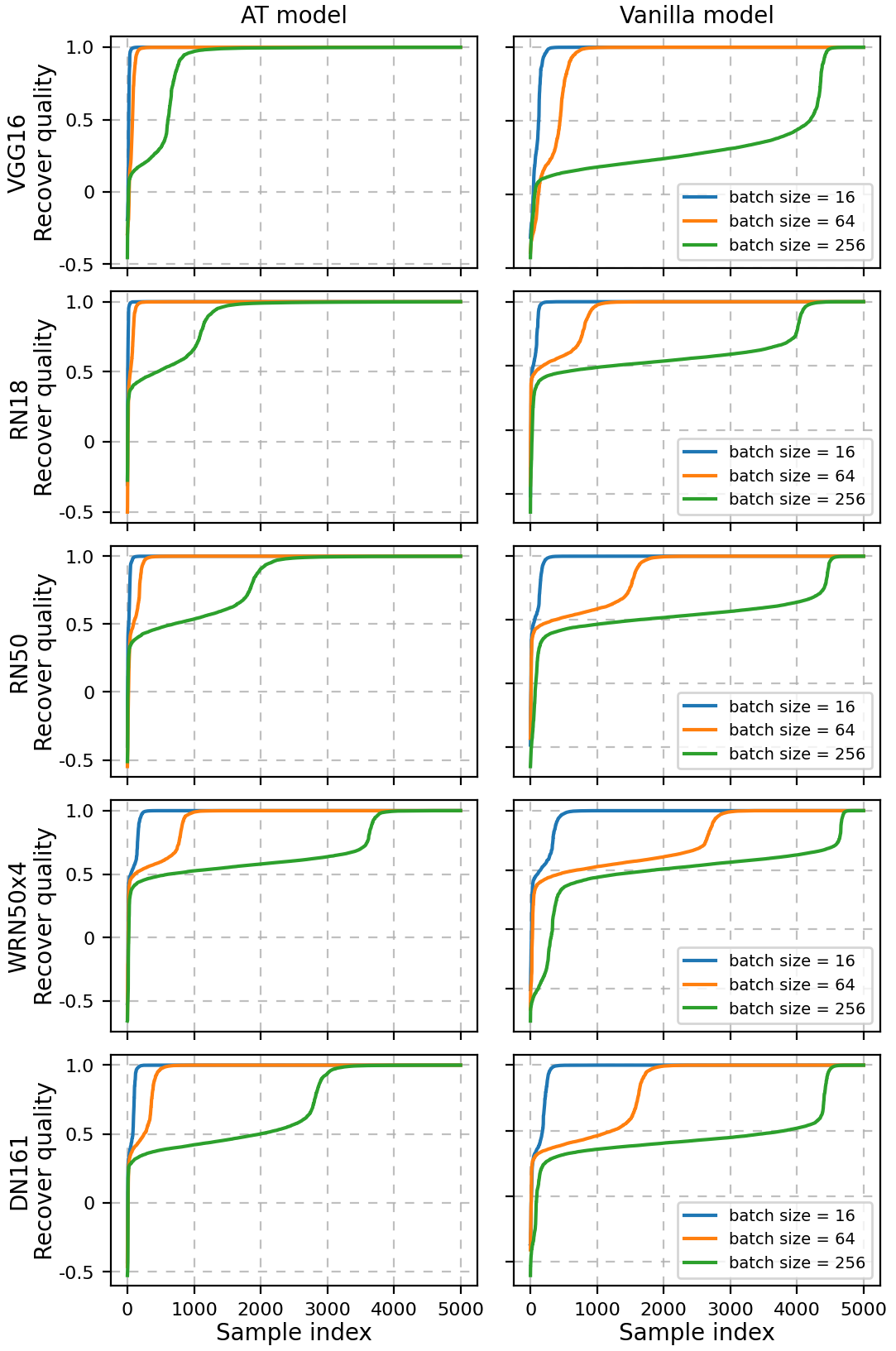
Figure 3: Feature restoration quality (in terms of cosine similarity) of the 5,000 anchor images on various AT and vanilla models and under various batch size. The samples are sorted by the recover quality in each plot. The closer the curve is to the upper left corner, the better feature restoration is achieved.

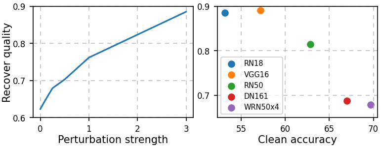
Figure 4: Left: Feature restoration quality v.s. the perturbation strength $\varepsilon$ of AT. RN18 is used here. Right: Feature restoration quality v.s. the model architecture. $\varepsilon=3.0$ is used here.

5.2 Feature restoration from gradients

We first evaluate our first attack step, namely feature restoration, for which the results are shown in Fig. 3. There are several key observations made from the results.

AT models enable better restoration of the features. Comparing the first and second column of Fig. 3, it is obvious that the feature restoration is much more successful on AT models than on vanilla models. For example, with RN18 architecture and a batch size of 256, there are around 3,500 out of 5,000 samples whose features can be restored nearly perfectly (i.e., with $\sim 1.0$ cosine similarity) on the AT model, while less than 1,000 samples’ features are restored that well on the vanilla model. This observation aligns with our analysis in Sec. 4.2.

In the left plot of Fig. 4, we also observe that the feature restoration quality (averaged over 5,000 samples) becomes better as the AT’s perturbation strength $\varepsilon$ increases, which further demonstrates that AT makes the model more vulnerable to the feature restoration attack step.

Feature restoration works even under large batch size. As discussed earlier, the motivation of the feature restoration step is to decouple the fused information of each individual input from the batch-averaged gradients. Indeed, we find this strategy effective even under a large batch size. Specifically, under the batch size of 256, the attack applied to an AT model can perfectly restore the features of at least 1,000 samples (with WRN50x4) and up to 4,000 samples (with VGG16), out of the total 5,000 samples. Not surprisingly, the restoration quality is even better when the batch size is smaller.

Models with smaller capacity are more vulnerable. In the right plot of Fig. 4, we visualize the feature restoration quality (averaged over 5,000 anchor samples) w.r.t. the test accuracy of various model architectures on the clean images of ImageNet. The general trend is that the models with lower clean accuracy is more vulnerable to the feature restoration attack step. We suspect that this is because the models with a smaller learning capacity (in terms of the clean accuracy) do not resist adversarial examples very well, and the probability $\bm{p}_{i,y_{i}}$ assigned to the ground-truth class of the adversarial input would be lower. As a result, small-capacity models could lead to better feature restoration (see Eq. 4).

5.3 Image reconstruction from features

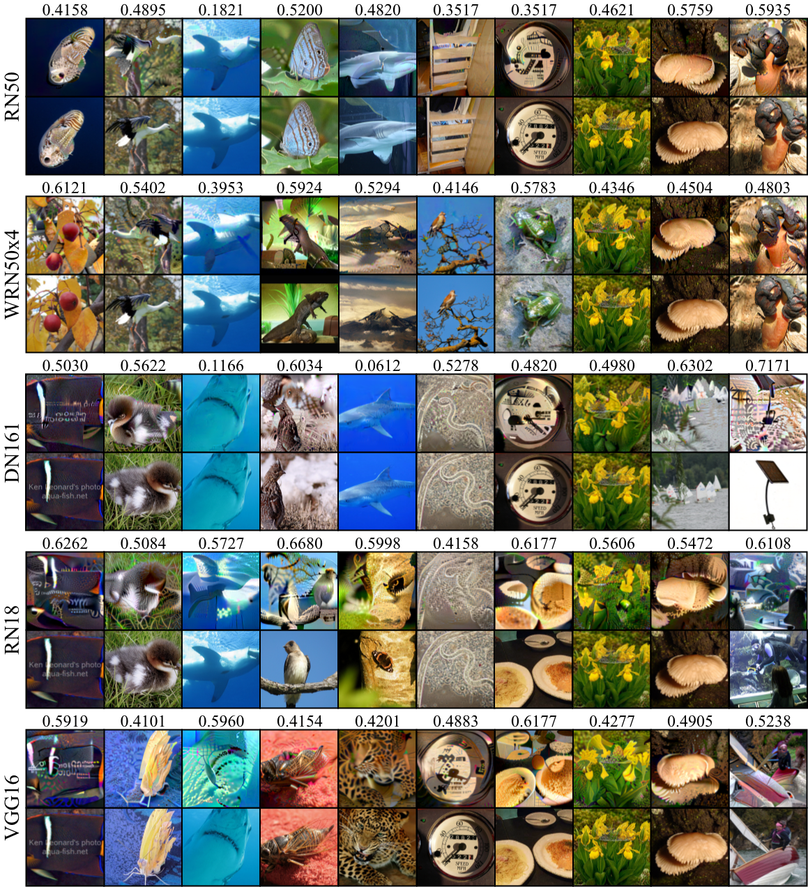
Figure 5: Visualization of reconstructed images on AT models (first row in each pair) and ground-truth ones (second row). The numbers are the LPIPS score ($\downarrow$).

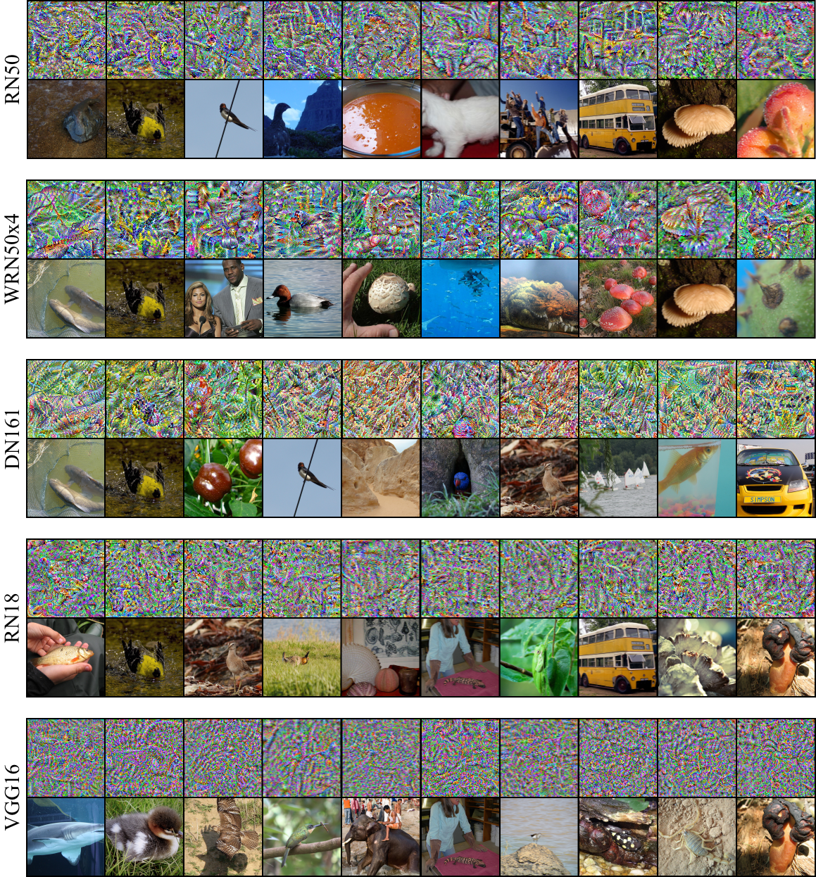
Figure 6: Visualization of reconstructed images on vanilla models (first row in each pair) and ground-truth ones (second row).

We next invert the restored features to recontruct input images according to Eq. 6. Specifically, we use Adam optimizer with a learning rate of 0.1 and perform 5,000 steps of optimization. The weight for the Total Variation loss $\mathcal{R}$ is $1e^{-6}$. Image generation is often sensitive to the initialization, and we find that using multiple random starts (and picking the best result according to the loss) can improve the image quality. Here we use 5 random starts.

We present the results obtained on AT models and vanilla models in Fig. 5 and Fig. 6, respectively. The takeaway here is twofold. First, AT models obviously enable much better reconstruction than vanilla models. Many of the generated images from AT models clearly unveil the object identity, often with accurate restoration of the visual details (e.g., the branches in the bird image obtained on WRN50x4). In comparison, vanilla models only yield absurd, hard-to-interpret patterns which hardly reveal useful information about the original images. Second, we find that the models with larger learning capacity are more suitable for the feature inversion. Recall that RN50, WRN50x4, and DN161 achieve higher clean accuracy than RN18 and VGG16 according to Fig. 4. In Fig. 5, the latter two models more often have distortions or unnatural patterns in their reconstructed images than the first three models. We suspect that this is because the large-capacity models can learn more semantic-meaningful features [3] during AT, which is essential for recovering the semantics of the original input images.

Finally, we remark that with AT models, our attack can better compromise the clients’ privacy than prior arts. Specifically, our method achieves an averaged LPIPS score of $0.4424$ on RN50 under a batch size of 256, while the current state-of-the-art method [19] obtained $0.4840$ under a batch size of 8 with the same model architecture. In addition, to our knowledge we are the first to report success of reconstruction under the batch size of 256 among the privacy attacks towards FL systems.

6 Conclusion

We develop a novel privacy attack against Adversarial Training models to break the privacy of Federated Learning systems. Evaluation demonstrates that our attack can accurately reconstruct the clients’ training images even when the batch size is large (up to 256). Thus, the clients that perform AT in the pursuit of robustness are in the same time putting their privacy at risk. By further exposing such robustness-privacy trade-off of AT models with a practical attack, we hope to motivate future studies to address this issue and develop some kind of privacy-aware AT.

References

- [1] Francesco Croce, Maksym Andriushchenko, Vikash Sehwag, Edoardo Debenedetti, Nicolas Flammarion, Mung Chiang, Prateek Mittal, and Matthias Hein. Robustbench: a standardized adversarial robustness benchmark. arXiv preprint arXiv:2010.09670, 2020.
- [2] Jia Deng, Wei Dong, Richard Socher, Li-Jia Li, Kai Li, and Li Fei-Fei. Imagenet: A large-scale hierarchical image database. In 2009 IEEE conference on computer vision and pattern recognition, pages 248–255. Ieee, 2009.
- [3] Logan Engstrom, Andrew Ilyas, Shibani Santurkar, Dimitris Tsipras, Brandon Tran, and Aleksander Madry. Adversarial robustness as a prior for learned representations. arXiv preprint arXiv:1906.00945, 2019.
- [4] Matt Fredrikson, Somesh Jha, and Thomas Ristenpart. Model inversion attacks that exploit confidence information and basic countermeasures. In Proceedings of the 22nd ACM SIGSAC conference on computer and communications security, pages 1322–1333, 2015.
- [5] Jonas Geiping, Hartmut Bauermeister, Hannah Dröge, and Michael Moeller. Inverting gradients - how easy is it to break privacy in federated learning? In H. Larochelle, M. Ranzato, R. Hadsell, M. F. Balcan, and H. Lin, editors, Advances in Neural Information Processing Systems, volume 33, pages 16937–16947. Curran Associates, Inc., 2020.
- [6] Kaiming He, Xiangyu Zhang, Shaoqing Ren, and Jian Sun. Deep residual learning for image recognition. In Proceedings of the IEEE conference on computer vision and pattern recognition, pages 770–778, 2016.
- [7] Gao Huang, Zhuang Liu, Laurens Van Der Maaten, and Kilian Q Weinberger. Densely connected convolutional networks. In Proceedings of the IEEE conference on computer vision and pattern recognition, pages 4700–4708, 2017.
- [8] Nitish Shirish Keskar, Dheevatsa Mudigere, Jorge Nocedal, Mikhail Smelyanskiy, and Ping Tak Peter Tang. On large-batch training for deep learning: Generalization gap and sharp minima. In 5th International Conference on Learning Representations, ICLR 2017, Toulon, France, April 24-26, 2017, Conference Track Proceedings. OpenReview.net, 2017.
- [9] Aleksander Madry, Aleksandar Makelov, Ludwig Schmidt, Dimitris Tsipras, and Adrian Vladu. Towards deep learning models resistant to adversarial attacks. In 6th International Conference on Learning Representations, ICLR 2018, Vancouver, BC, Canada, April 30 - May 3, 2018, Conference Track Proceedings. OpenReview.net, 2018.
- [10] Aravindh Mahendran and Andrea Vedaldi. Understanding deep image representations by inverting them. In Proceedings of the IEEE conference on computer vision and pattern recognition, pages 5188–5196, 2015.
- [11] Brendan McMahan, Eider Moore, Daniel Ramage, Seth Hampson, and Blaise Aguera y Arcas. Communication-efficient learning of deep networks from decentralized data. In Artificial intelligence and statistics, pages 1273–1282. PMLR, 2017.
- [12] Felipe A Mejia, Paul Gamble, Zigfried Hampel-Arias, Michael Lomnitz, Nina Lopatina, Lucas Tindall, and Maria Alejandra Barrios. Robust or private? adversarial training makes models more vulnerable to privacy attacks. arXiv preprint arXiv:1906.06449, 2019.
- [13] Hadi Salman, Andrew Ilyas, Logan Engstrom, Ashish Kapoor, and Aleksander Madry. Do adversarially robust imagenet models transfer better? Advances in Neural Information Processing Systems, 33:3533–3545, 2020.
- [14] Reza Shokri, Marco Stronati, Congzheng Song, and Vitaly Shmatikov. Membership inference attacks against machine learning models. In 2017 IEEE symposium on security and privacy (SP), pages 3–18. IEEE, 2017.
- [15] Karen Simonyan and Andrew Zisserman. Very deep convolutional networks for large-scale image recognition. arXiv preprint arXiv:1409.1556, 2014.
- [16] Liwei Song, Reza Shokri, and Prateek Mittal. Privacy risks of securing machine learning models against adversarial examples. In Proceedings of the 2019 ACM SIGSAC Conference on Computer and Communications Security, pages 241–257, 2019.
- [17] Christian Szegedy, Wojciech Zaremba, Ilya Sutskever, Joan Bruna, Dumitru Erhan, Ian J. Goodfellow, and Rob Fergus. Intriguing properties of neural networks. In Yoshua Bengio and Yann LeCun, editors, 2nd International Conference on Learning Representations, ICLR 2014, Banff, AB, Canada, April 14-16, 2014, Conference Track Proceedings, 2014.
- [18] Florian Tramer, Nicholas Carlini, Wieland Brendel, and Aleksander Madry. On adaptive attacks to adversarial example defenses. Advances in Neural Information Processing Systems, 33:1633–1645, 2020.
- [19] Hongxu Yin, Arun Mallya, Arash Vahdat, Jose M Alvarez, Jan Kautz, and Pavlo Molchanov. See through gradients: Image batch recovery via gradinversion. In Proceedings of the IEEE/CVF Conference on Computer Vision and Pattern Recognition, pages 16337–16346, 2021.
- [20] Sergey Zagoruyko and Nikos Komodakis. Wide residual networks. In Edwin R. Hancock Richard C. Wilson and William A. P. Smith, editors, Proceedings of the British Machine Vision Conference (BMVC), pages 87.1–87.12. BMVA Press, September 2016.
- [21] Hongyang Zhang, Yaodong Yu, Jiantao Jiao, Eric Xing, Laurent El Ghaoui, and Michael Jordan. Theoretically principled trade-off between robustness and accuracy. In International conference on machine learning, pages 7472–7482. PMLR, 2019.
- [22] Richard Zhang, Phillip Isola, Alexei A Efros, Eli Shechtman, and Oliver Wang. The unreasonable effectiveness of deep features as a perceptual metric. In Proceedings of the IEEE conference on computer vision and pattern recognition, pages 586–595, 2018.
- [23] Bo Zhao, Konda Reddy Mopuri, and Hakan Bilen. idlg: Improved deep leakage from gradients. arXiv preprint arXiv:2001.02610, 2020.
- [24] Ligeng Zhu and Song Han. Deep leakage from gradients. In Federated learning, pages 17–31. Springer, 2020.