SUPPLEMENTARY MATERIAL

 

 

S1 Scattering parameters for a transmission measurement

Just as the load impedance determines the reflection amplitude in a reflectometry experiment (Eq. (10)), it also determines the scattering amplitudes in a transmission experiment. The two simplest transmission circuits are shown in Fig. S1. The amplitude for transmission through an impedance $Z_{\mathrm{load}}$ (Fig. S1(a)) is

$$T=\frac{2Z_{\mathrm{0}}}{2Z_{\mathrm{0}}+Z_{\mathrm{load}}}.$$ (S1)

The amplitude for transmission past an impedance $Z_{\mathrm{load}}$ (Fig. S1(b)) is

$$T=\frac{2Z_{\mathrm{load}}}{2Z_{\mathrm{load}}+Z_{\mathrm{0}}}.$$ (S2)

Examples of rf-SETs measured in a transmission configuration are Refs. Hirayama2000, fujisawa2000_transmission.

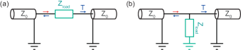
Figure S1: The simplest geometries for a transmission measurement. (a) Transmission through an impedance. (b) Transmission past an impedance.

S2 The series equivalent of a reflectrometry resonator; derivation of Equation (42) of the main text

Here, we demonstrate the approximate equivalence between the reflectometry circuit of Fig. 7(a), described by Eq. (40), and its series model in Fig. 7(b), described by Eq. (42). We do this by showing that they have the same impedance near resonance.

First, we write explicitly the real and imaginary parts of Eq. (40):

$$Z_{\mathrm{load}}=j\omega L_{\mathrm{C}}+R_{\mathrm{L}}+\frac{R_{\mathrm{eq}}}{1+\omega^{2}R_{\mathrm{eq}}^{2}C_{\mathrm{P}}^{2}}-j\omega\frac{R_{\mathrm{eq}}^{2}C_{\mathrm{P}}}{1+\omega^{2}R_{\mathrm{eq}}^{2}C_{\mathrm{P}}^{2}}$$ (S3)

In the limit $\omega R_{\mathrm{eq}}C_{\mathrm{P}}\gg 1$, which is true for most applications, we obtain:

$$Z_{\mathrm{load}}=R_{\mathrm{L}}+\frac{1}{\omega^{2}R_{\mathrm{eq}}C_{\mathrm{P}}^{2}}+j\omega L_{\mathrm{C}}+\frac{1}{j\omega C_{\mathrm{P}}}.$$ (S4)

The resonant angular frequency $\omega_{\mathrm{r}}=1/\sqrt{L_{\mathrm{C}}C_{\mathrm{P}}}$ can be found by setting the imaginary part of Eq. (S4) equal to zero.

Finally, to see the equivalence between the reflectometry circuit on resonance and a standard RLC circuit, substitute the resonant frequency into Eq. (S4), to find the effective resistance:

$$R_{\mathrm{eff}}=\frac{L_{\mathrm{C}}}{C_{\mathrm{P}}R_{\mathrm{eq}}}+R_{\mathrm{L}},$$ (S5)

which implies that near the resonance frequency, the reflectometry circuit behaves like an series RLC circuit with impedance

$$Z_{\mathrm{load}}=R_{\mathrm{eff}}+j\omega L_{\mathrm{C}}+\frac{1}{j\omega C_{\mathrm{P}}}.$$ (S6)

S3 Using spectral densities

In this section, we summarise how to calculate and use a spectral density, with a focus on quantitative experimental analysis. Two excellent explanations of how to understand and use spectral densities are the review article by Clerk et al. [Clerk2010], written from a theoretical physics perspective, and the textbook by Press et al. [Press2007], written from a computer science perspective. Unfortunately nomenclature differs in many ways between these two fields, and both differ from the conventions of electronic engineering, represented e.g. by the textbook of Horowitz and Hill [Horowitz2015]. Infuriating scaling factors proliferate, and some of them are infinite. Here we present a self-consistent pedagogical treatment, written from an experimentalist’s perspective and including brief derivations and examples, of how to calculate a spectral density and use it to estimate uncertainty in a measurement.

The spectral density $S_{VV}[f]$ represents the intensity of a signal $V(t)$ near frequency $f$. This representation involves some choices. We make the following choices in order to make our spectral densities consistent with what appears on the screen of your spectrum analyser:

1. The signal $V(t)$ is assumed to be real and classical.

2. The spectral density of a voltage signal is defined by Eq. (134), giving units $\mathrm{V}^{2}\mathrm{s}$. Some authors [Press2007] call this “power spectral density per unit time.”

3. The spectral density is one-sided, which means that it is defined for both positive and negative $f$ but is normalised so that $\int_{0}^{\infty}S_{VV}[f]\,df=\langle V^{2}(t)\rangle$.

With these conventions, we will show how to calculate a spectral density in different situations, and how to use it for its most valuable purpose, which is to derive uncertainties in measured quantities.

Recognizing and converting between definitions of the spectral density
Here’s our cheat sheet for converting between conventions for the classical spectral density. It covers most of the definitions we have encountered. (a) This Review follows the one-sided convention common among experimentalists, in which the factors in Eqs. (S24-S25) are chosen so that $${{\langle}}V^{2}(t){{\rangle}}=\int_{0}^{\infty}S_{VV}[f]\,df.$$ (S7) In this convention the Wiener-Khinchin theorem, i.e. the inverse of Eq. (S26), is $$S_{VV}[f]=2\int_{-\infty}^{\infty}{{\langle}}V(0)V(\tau){{\rangle}}e^{-2\pi if\tau}\,d\tau.$$ (S8) The noise density $e_{\mathrm{n}}$ used by electrical engineers [Horowitz2015] is $$e_{\mathrm{n}}^{2}[f]=S_{VV}^{\mathrm{N}}[f].$$ (S9) (b) In the one-sided convention using angular frequency, the spectral density $S_{VV}^{\prime}$ satisfies $\displaystyle{{\langle}}V^{2}(t){{\rangle}}$ $\displaystyle=\int_{0}^{\infty}S^{\prime}_{VV}[\omega]\,\frac{d\omega}{2\pi}$ (S10) $\displaystyle S^{\prime}_{VV}[\omega]$ $\displaystyle=2\int_{-\infty}^{\infty}{{\langle}}V(0)V(\tau){{\rangle}}e^{-i\omega\tau}\,d\tau.$ (S11) To convert from our convention, use $$S^{\prime}_{VV}[\omega]=S_{VV}\left[\frac{\omega}{2\pi}\right].$$ (S12) (c) In the two-sided convention using frequency, $\displaystyle{{\langle}}V^{2}(t){{\rangle}}$ $\displaystyle=\int_{-\infty}^{\infty}S^{\prime}_{VV}[f]\,df,$ (S13) $\displaystyle S^{\prime}_{VV}[f]$ $\displaystyle=\int_{-\infty}^{\infty}{{\langle}}V(0)V(\tau){{\rangle}}e^{-2\pi if\tau}\,d\tau.$ (S14) and the conversion is $$S^{\prime}_{VV}[f]=\frac{1}{2}S_{VV}[f].$$ (S15)       (d) In the two-sided convention using angular fre- quency, which is common among theorists [Clerk2010], $\displaystyle{{\langle}}V^{2}(t){{\rangle}}$ $\displaystyle=\int_{-\infty}^{\infty}S^{\prime}_{VV}[\omega]\,\frac{d\omega}{2\pi},$ (S16) $\displaystyle S^{\prime}_{VV}[\omega]$ $\displaystyle=\int_{-\infty}^{\infty}{{\langle}}V(0)V(\tau){{\rangle}}e^{-i\omega\tau}\,d\tau.$ (S17) with $$S^{\prime}_{VV}[\omega]=\frac{1}{2}S_{VV}\left[\frac{\omega}{2\pi}\right].$$ (S18) (e) In the two-sided convention using angular frequency and normalised over $\omega$, $\displaystyle{{\langle}}V^{2}(t){{\rangle}}$ $\displaystyle=\int_{-\infty}^{\infty}S^{\prime}_{VV}[\omega]\,d\omega,$ (S19) $\displaystyle S^{\prime}_{VV}[\omega]$ $\displaystyle=\frac{1}{2\pi}\int_{-\infty}^{\infty}{{\langle}}V(0)V(\tau){{\rangle}}e^{-i\omega\tau}\,d\tau.$ (S20) with $$S^{\prime}_{VV}[\omega]=\frac{1}{4\pi}\,S_{VV}\left[\frac{\omega}{2\pi}\right].$$ (S21) (f) In the one-sided computer science convention [Press2007], the “power spectral density” $P_{V}[f]$ is defined such that $$S_{VV}[f]=\lim_{T\rightarrow\infty}\Braket{\frac{1}{T}\,P_{V}[f]}$$ (S22) where $T$ is the measurement duration, meaning that $$\lceil V^{2}(t)\rceil=\frac{1}{T}\int_{0}^{\infty}P_{V}[f]\,df.$$ (S23) where $\lceil\cdot\rceil$ denotes a time average. Confusingly, $P_{V}[f]$ has units $\mathrm{V}^{2}\,\mathrm{s}^{2}$, which means it’s neither a power nor a density per unit frequency. A final freedom is the sign of the exponent in Eq. (S8). Fortunately, if $V(t)$ is real, both choices give the same $S_{VV}[f]$. Most papers containing spectral densities either state their convention as one-sided or two-sided, or else define $S_{VV}$ by an equation similar to Eq. (S8) by which their convention is implied. However, some contain more subtle clues, or even no clues at all. If anything here was of service to you, we implore you to play your part in ending this misery: Whenever you use a spectral density, say clearly how it is defined.

S3.1 How to calculate a spectral density

Suppose our experiment is generating a voltage $V(t)$. How do we calculate its spectral density $S_{VV}[f]$? We will answer this question by presenting the definition of $S_{VV}[f]$ in terms of a Fourier integral. Under nearly all practical conditions, this definition implies Eq. (134) of the main text. We will prove this statement and discuss when it holds. We then explain how to estimate the Fourier integral in different situations.

S3.1.1 Definition of $S_{VV}[f]$ in terms of a Fourier integral

The one-sided spectral density is defined as

$$S_{VV}(f)~{}\text{or}~{}S_{VV}[f]\equiv 2\lim_{T\rightarrow\infty}\langle|V_{\mathrm{T}}[f]|^{2}\rangle$$ (S24)

where

$$V_{\mathrm{T}}[f]\equiv\frac{1}{\sqrt{T}}\int_{-T/2}^{T/2}V(t)e^{-2\pi ift}dt.$$ (S25)

is the windowed Fourier transform. Since $V(t)$ is real, we have $S_{VV}[f]=S_{VV}[-f]$.

As noted, there is more than one way to define the spectral density. The most common conventions are summarised in the box overleaf.

S3.1.2 When the two expressions for $S_{VV}[f]$ are equivalent

We take Eq. (S24) to define the spectral density, but Eq. (134) is more intuitive. Here we explain when the first expression implies the second.

Suppose $V(t)$ is stationary, which means that its statistical properties are independent of time. (We return shortly to the question of when this is true.) Then its spectral density, defined by Eq. (S24), obeys the Wiener-Khinchin theorem, which states that $S_{VV}[f]$ is related to the autocorrelation function through a Fourier transform:

$${{\langle}}V(t)V(t^{\prime}){{\rangle}}=\frac{1}{2}\int_{-\infty}^{\infty}df\,e^{2\pi if(t-t^{\prime})}S_{VV}[f].$$ (S26)

Now apply this to the filtered voltage $\mathbb{V}(t)$ of Eq. (134), from which all spectral components of $V(t)$ have been removed except those within a small bandwidth $B_{f}$ of $f$. The Wiener-Khinchin theorem now gives

$${{\langle}}\mathbb{V}(t)\mathbb{V}(t^{\prime}){{\rangle}}=\int_{f-B_{f}/2}^{f+B_{f}/2}df^{\prime}\,e^{2\pi if^{\prime}(t-t^{\prime})}S_{VV}[f^{\prime}],$$ (S27)

where we have also used that $S_{VV}[f]=S_{VV}[-f]$. Setting $t^{\prime}=t$ and dividing both sides by $B_{f}$ leads to

$$\frac{{{\langle}}\mathbb{V}^{2}(t){{\rangle}}}{B_{f}} =\frac{1}{B_{f}}\int_{f-B_{f}/2}^{f+B_{f}/2}df^{\prime}\,S_{VV}[f^{\prime}]$$ (S28)

In the limit $B_{f}\rightarrow 0$ this becomes

$$S_{VV}[f] =\lim_{B_{f}\rightarrow 0}\frac{{{\langle}}\mathbb{V}^{2}(t){{\rangle}}}{B_{f}}$$ (S29)

$$=\lim_{B_{f}\rightarrow 0}\frac{{\lceil\langle}\mathbb{V}^{2}(t){\rangle\rceil}}{B_{f}}.$$ (S30)

where the second equality follows because $V(t)$ is stationary and therefore the time average $\lceil\cdot\rceil$ does not change the right hand side. This is identical to Eq. (134) in the main text.

What about a non-stationary $V(t)$? For example, $V(t)=A\cos(2\pi f_{0}t)$ is clearly non-stationary because its variance depends on time as ${{\langle}}V^{2}(t){{\rangle}}\propto\cos^{2}(2\pi f_{0}t)$. Does Eq. (S30) hold for such an observable? Although we cannot use our argument based on Eq. (S26), we show below Eq. (S37) that any signal that can be represented as a Fourier series nevertheless obeys Eq. (S30). Thus we have proved Eq. (134) in the main text, provided that $V(t)$ is either stationary or a Fourier series.

These two cases cover many observables that are encountered experimentally . The reason that most observables, especially noise, are stationary is time translation invariance; once an experiment has been running for a long time, its behavior should not depend on when it was turned on. As we shall see in Section S3.2, this is an extremely useful property when estimating measurement uncertainty. Unfortunately it is not always true, even for noise: an obvious counterexample is a constant drift in experimental parameters. Such non-stationary noise is not accurately described by a spectral density, and indeed the right-hand side of Eq. (S24) may not be mathematically defined.

S3.1.3 Evaluating the Fourier integral

Equation (S24) defines the spectral density $S_{VV}[f]$, but is not directly useful for calculating it in a real experiment, where we cannot wait for infinite $T$ and we may not have access to multiple iterations. In that case we should use the following approximation to Eq. (S24):

$$S_{VV}[f]\approx 2|V_{\mathrm{T}}[f]|^{2}.$$ (S31)

with $V_{\mathrm{T}}[f]$ given by Eq. (S25).

Often Eq. (S31) is still insufficient because we do not have a continuous record $V(t)$, but instead a series of samples $V(t_{k})$ taken at regular instants $t_{k}$ separated by a sampling interval $\Delta$. Now we must be careful, because frequency components separated by the Nyquist frequency $1/2\Delta$ are indistinguishable in the sampled record. A high-frequency component of $V(t)$ may therefore appear spuriously at a lower frequency in the calculated spectrum, an effect known as aliasing. For this reason, before digitising any signal, it should be filtered using a low-pass filter with a cutoff below the Nyquist frequency. If this has been done, the spectral density is [Press2007]:

$$S_{VV}[f]\approx 2\frac{\Delta^{2}}{T}\langle|V_{\mathrm{D}}[f]|^{2}\rangle$$ (S32)

where the discrete Fourier transform of $V(t_{k})$ is:

$$V_{\mathrm{D}}[f]\equiv\sum_{k=0}^{N-1}V(t_{k})e^{-2\pi ikf\Delta}.$$ (S33)

If only one iteration of the measurement is available, we must omit the expectation value in Eq. (S32).

Lastly, we may need to calculate the spectral density of a mathematical function $V(t)$ that is known for all values of $t$. If $V(t)$ is stationary, then Eq. (S26) leads to:

$$S_{VV}[f]=2\int_{\infty}^{\infty}{{\langle}}V[f]V[f^{\prime}]{{\rangle}}\,df^{\prime}$$ (S34)

where $V[f]\equiv\int_{-\infty}^{\infty}V(t)e^{-2\pi ift}dt$ is the conventional Fourier transform.

If not, then Eq. (S24) needs to be evaluated directly. A useful case is the Fourier series

$$V(t)=\sum_{n}A_{n}\cos(2\pi f_{n}t)+B_{n}\sin(2\pi f_{n}t)$$ (S35)

with $A_{n}$ and $B_{n}$ real. The corresponding spectral density is

$$S_{VV}[f]=\sum_{n}({{\langle}}A_{n}^{2}{{\rangle}}+{{\langle}}B_{n}^{2}{{\rangle}})\,\frac{\delta[f+f_{n}]+\delta[f-f_{n}])}{2}.$$ (S36)

If the voltage in Eq. (S35) is filtered around a single frequency $f$, then clearly

$${\lceil\langle}\mathbb{V}^{2}{\rangle\rceil}=\frac{1}{2}({{\langle}}A_{n}^{2}{{\rangle}}+{{\langle}}B_{n}^{2}{{\rangle}})(\delta[f+f_{n}]+\delta[f-f_{n}]),$$ (S37)

in agreement with Eq. (S36) and Eq. (S30).

S3.2 How to derive a measurement uncertainty from the spectral density

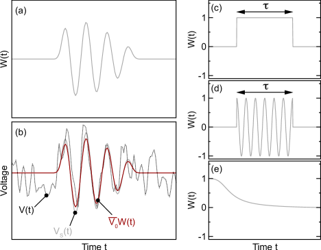
Figure S2: Using a window function to estimate an observable. (a) Example of a window function, proportional to the noise-free signal. (b) Typical measured signal $V(t)$, including noise, arising from an underlying signal $V_{\mathrm{S}}(t)$. Applying Eq. (S40) leads to an estimate of the signal amplitude $\overline{V_{0}}$ and a reconstructed signal $\overline{V_{0}}W(t)$. (c-e) Examples of weighting functions for (c) averaging a dc voltage (Eq. (S39)); (d) estimating the amplitude of an oscillating voltage (Eq. (S63)); (e) high-fidelity qubit readout [Gambetta2007].

S3.2.1 Uncertainty in measuring a voltage

As stated in Section VI A 3, a valuable property of the spectral density is that it determines the uncertainty of a measurement in the presence of noise. Let us explain how this is done. In general, electrical measurements transduce the observable of interest (for example qubit state, displacement, temperature, or impedance) into a voltage $V_{\mathrm{S}}(t)$ contaminated by noise $V_{\mathrm{N}}(t)$. From a record of $V(t)=V_{\mathrm{S}}(t)+V_{\mathrm{N}}(t)$, acquired over a duration $\tau$, it is our task to extract the observable with an associated uncertainty or error bar.

A general model of this process is shown in Fig. S2. We expect the signal to be

$$V_{\mathrm{S}}(t)=V_{0}\,W(t),$$ (S38)

where $V_{0}$ is proportional to the observable and $W(t)$ is a weighting function. Figure S2(a) shows an example of such a weighting function. For example, if we are measuring a constant voltage then

$$W(t)=\begin{cases}1&\text{if}\ 0<t<\tau\\ 0&\text{otherwise}\end{cases}$$ (S39)

as in Fig. S2(c).

The optimal estimate $\overline{V_{0}}$ can be derived using a least-squares fit [Press2007]. In other words, we choose $\overline{V_{0}}$ to minimise the integrated squared difference between the model and the data. This implies that

$$\frac{\partial}{\partial\overline{V_{0}}}\int_{-\infty}^{\infty}(V(t)-\overline{V_{0}}\,W(t))^{2}\,dt=0$$ (S40)

where

$$V(t)=V_{0}W(t)+V_{\mathrm{N}}(t)$$ (S41)

is the measured voltage trace including noise. Solving Eq. (S40) gives

$$\overline{V_{0}}=\frac{1}{\tau_{W}}\int_{-\infty}^{\infty}V(t)\,W(t)\,dt,$$ (S42)

where

$$\tau_{W}\equiv\int_{-\infty}^{\infty}W^{2}(t)\,dt$$ (S43)

is a normalisation factor which can be thought of as the weighted duration of the measurement. Equation. (S40) provides an optimal estimate of $V_{0}$ in the sense that the expectation value of $\overline{V_{0}}$ over many iterations is the true value:

$$\langle\overline{V_{0}}\rangle =\frac{1}{\tau_{W}}\int_{-\infty}^{\infty}\langle V_{0}W(t)+V_{\mathrm{N}}(t)\rangle\,W(t)\,dt$$ (S44)

$$=V_{0},$$ (S45)

since $\langle V_{\mathrm{N}}(t)\rangle=0$. (If not, $V_{\mathrm{N}}(t)$ is a correctable offset rather than noise).

Figure S2(b) shows an example of a “true” signal $V_{\mathrm{S}}(t)$ associated with the weighting function in Fig. S2(a), and one realisation of a measured signal $V(t)$. Applying Eq. (S42) to generate an estimate $\overline{V_{0}}$ leads to a reconstructed signal $\overline{V_{0}}W(t)$ which fairly accurately matches the “true” signal.

As this figure suggests and Eq. (S45) confirms, the procedure estimates the correct $\overline{V_{0}}$ on average. However, the value derived from any individual voltage trace has an uncertainty. This uncertainty is determined by the variance over a large number of estimates, each incorporating a different realisation of the random noise. To calculate this, we evaluate

$$\langle\overline{V_{0}}^{2}\rangle =\frac{1}{\tau_{W}^{2}}\left\langle\int_{-\infty}^{\infty}V(t)W(t)\,dt\int_{-\infty}^{\infty}V(t^{\prime})W(t^{\prime})\,dt^{\prime}\right\rangle$$ (S46)

$$=\frac{1}{\tau_{W}^{2}}\iint_{-\infty}^{\infty}dt\,dt^{\prime}\,\langle V(t)V(t^{\prime})\rangle\,W(t)W(t^{\prime})$$ (S47)

$$=\frac{1}{\tau_{W}^{2}}\iint_{-\infty}^{\infty}dt\,dt^{\prime}\,\langle(V_{0}W(t)+V_{\mathrm{N}}(t))(V_{0}W(t^{\prime})+V_{\mathrm{N}}(t^{\prime}))\rangle\,W(t)W(t^{\prime})$$ (S48)

$$=\frac{1}{\tau_{W}^{2}}\iint_{-\infty}^{\infty}dt\,dt^{\prime}\,\langle V_{0}^{2}W(t)W(t^{\prime})+V_{0}V_{\mathrm{N}}(t)W(t^{\prime})+V_{0}V_{\mathrm{N}}(t^{\prime})W(t)+V_{\mathrm{N}}(t)V_{\mathrm{N}}(t^{\prime})\rangle\,W(t)W(t^{\prime})$$ (S49)

$$=\frac{1}{\tau_{W}^{2}}\iint_{-\infty}^{\infty}dt\,dt^{\prime}\,(V_{0}^{2}W(t)W(t^{\prime})+V_{0}\langle V_{\mathrm{N}}(t)\rangle W(t^{\prime})+V_{0}\langle V_{\mathrm{N}}(t^{\prime})\rangle W(t)+\langle V_{\mathrm{N}}(t)V_{\mathrm{N}}(t^{\prime})\rangle\,W(t)W(t^{\prime})).$$ (S50)

Here the first line is a substitution from Eq. (S42), the second line follows by rearrangement, the third line by substituting from Eq. (S41), the fourth line by expanding the brackets, and the fifth line follows because the expectation values need to be taken only over combinations of $V_{\mathrm{N}}(t)$, which are the only stochastic terms. Since the expectation value of $V_{\mathrm{N}}(t)$ is zero, Eq. (S50) simplifies to:

$$\begin{split}\langle\overline{V_{0}}^{2}\rangle&=\frac{1}{\tau_{W}^{2}}\iint_{-\infty}^{\infty}dt\,dt^{\prime}\,V_{0}^{2}W^{2}(t)W^{2}(t^{\prime})\\ &\qquad\qquad+\langle V_{\mathrm{N}}(t)V_{\mathrm{N}}(t^{\prime})\rangle\,W(t)W(t^{\prime})\\ \end{split}$$ (S51)

$$=V_{0}^{2}+\frac{1}{\tau_{W}^{2}}\iint_{-\infty}^{\infty}dt\,dt^{\prime}\,\langle V_{\mathrm{N}}(t)V_{\mathrm{N}}(t^{\prime})\rangle\,W(t)W(t^{\prime}).$$ (S52)

To proceed further, we need to assume that $V_{\mathrm{N}}(t)$ is stationary. Our justification is discussed at the end of Section S3.1.2. If we do this, we can evaluate Eq. (S52) using the Wiener-Khinchin theorem (Eq. (S26)). The double integral becomes

$$\iint_{-\infty}^{\infty}dt\,dt^{\prime}\int_{-\infty}^{\infty}df\,e^{2\pi if(t-t^{\prime})}S_{VV}^{\mathrm{N}}[f]W(t)W(t^{\prime})$$

$$=\int_{-\infty}^{\infty}df\,S_{VV}^{\mathrm{N}}[f]\int_{-\infty}^{\infty}dt\,e^{2\pi ift}W(t)\int_{-\infty}^{\infty}dt\,e^{-2\pi ift^{\prime}}W(t^{\prime})$$ (S53)

$$=\int_{-\infty}^{\infty}df\,S_{VV}^{\mathrm{N}}[f]\,W[-f]W[f]$$ (S54)

$$=\int_{-\infty}^{\infty}df\,S_{VV}^{\mathrm{N}}[f]\,|W[f]|^{2}$$ (S55)

where $W[f]$ is the Fourier transform of $W(t)$. The first equation follows by rearrangement, the second equation follows from the definition of the Fourier transform, and the third equation follows because $W(t)$ is real and therefore $W[-f]=(W[f])^{*}$.

Finally, Eqs. (S45), (S52), and (S55) can be combined to give a compact expression for the variance of the estimate $\overline{V_{0}}$:

$$\mathrm{var}(\overline{V_{0}}) \equiv\langle\overline{V_{0}}^{2}\rangle-\langle\overline{V_{0}}\rangle^{2}$$ (S56)

$$=\frac{1}{\tau_{W}^{2}}\int_{0}^{\infty}df\,S_{VV}^{\mathrm{N}}[f]\,|W[f]|^{2}.$$ (S57)

The uncertainty in the measured parameter $V_{0}$ is

$$\sigma(\overline{V_{0}})=\sqrt{\mathrm{var}(\overline{V_{0}})}.$$ (S58)

Equation (S57) is intuitive because the uncertainty is determined by the overlap between the noise spectral density $S_{VV}^{\mathrm{N}}[f]$ and the spectral weighting of the expected signal $|W[f]|^{2}$. This is the fundamental relationship between the spectral density of stationary noise and the corresponding measurement uncertainty.

S3.2.2 Example 1: Uncertainty from a measurement with fixed duration

Calculating the uncertainty is now a matter of choosing the appropriate weighting function $W[f]$ in Eq. (S57). For example, consider the measurement described by Eqs. (135a) and (135b) in the main text, in which $\overline{V_{0}}$ must be estimated from a measurement of fixed duration $\tau$. If we are measuring a constant voltage, i.e. using $W(t)$ given by Eq. (S39), then we find:

$$\tau_{W} =\tau$$ (S59)

$$|W[f]|^{2} =\tau^{2}\left(\frac{\sin(\pi\tau f)}{\pi\tau f}\right)^{2}$$ (S60)

and therefore

$$\mathrm{var}(\overline{V_{0}}) =\int_{0}^{\infty}df\,\left(\frac{\sin(\pi\tau f)}{\pi\tau f}\right)^{2}S_{VV}^{\mathrm{N}}[f]$$ (S61)

$$\approx\frac{1}{2\tau}S_{VV}^{\mathrm{N}}[0],$$ (S62)

where the approximation holds provided that $S_{VV}^{\mathrm{N}}[f]$ is smooth near the origin where $|W[f]|^{2}$ is large. This is Eq. (124a) in the main text.

If we are measuring an oscillating voltage such as Eq. (139) in the main text, then the appropriate window function is

$$W(t)=\begin{cases}\cos(2\pi f_{0}t)&\text{if}\ 0<t<\tau\\ 0&\text{otherwise},\end{cases}$$ (S63)

as in Fig. S2(b). If we can average over many cycles of the oscillation, i.e. $f_{0}\tau\gg 1$, then

$$\tau_{W} \approx\frac{\tau}{2}$$ (S64)

$$|W[f]|^{2} \approx\frac{\tau^{2}}{4}\left(\delta[f-f_{0}]+\delta[f+f_{0}]\right)$$ (S65)

and therefore

$$\mathrm{var}(\overline{V_{0}})\approx\frac{1}{\tau}S_{VV}^{\mathrm{N}}[f_{0}]$$ (S66)

This leads to Eq. (140b).

S3.2.3 Example 2: Uncertainty from a measurement using a frequency filter

Another common situation is that we have filtered the voltage record using a filter with amplitude transmission $F[f]$. The filtered record can be regarded as a measurement of the underlying signal $V_{\mathrm{S}}(t)$. What is the uncertainty of this measurement?

If the Fourier transform of the original voltage is $V[f]$, the Fourier transform of the filtered signal is

$$\mathbb{V}[f]=F[f]V[f],$$ (S67)

or equivalently

$$\mathbb{V}(t)=\int_{-\infty}^{\infty}V(u)F(t-u)\,du$$ (S68)

where $u$ is a time interval and $F(u)$ is the inverse Fourier transform of $F[f]$. (Obviously a causal filter has $F(t-u)=0$ for $t<u$.) This is the process that generates the low-pass filtered traces in Fig. 24(d).

Equation (S68) has the same form as Eq. (S42), except that $W(u)$ has been replaced by a new weighting function $\tau_{W}F(t-u)$. The filtered voltage $\mathbb{V}(t)$ is thus an estimate of $V_{\mathrm{S}}(t)$. Although the estimate may not be optimal in the sense of Eq. (S45), a sensibly chosen filter often gets pretty close, meaning that the error is dominated by fluctuations due to $V_{\mathrm{N}}(t)$ rather than by distortion of $V_{\mathrm{S}}(t)$ due to the filter.

Provided this is true, then the measurement uncertainty can be calculated by the same procedure as led to Eq. (S57), giving

$$\mathrm{var}(\mathbb{V}(t)-\mathbb{V}_{\mathrm{S}}(t)) =\int_{0}^{\infty}df\,S_{VV}^{\mathrm{N}}[f]\,|F[f]|^{2}$$ (S69)

$$\approx B_{f}\,S_{VV}^{\mathrm{N}}[f_{0}]$$ (S70)

where the approximation holds provided the noise spectrum is smooth across the filter passband. Here $\mathbb{V}_{\mathrm{S}}(t)\approx V_{\mathrm{S}}(t)$ is the filtered signal voltage, $f_{0}$ is the center frequency of the filter, and

$$B_{f}\equiv\int_{0}^{\infty}|F[f]|^{2}\,df$$ (S71)

is its equivalent noise bandwidth. As above, the uncertainty is the square root of Eq. (S71).

In terms of the windowing function in the time domain associated with a filter in the frequency domain, the equivalent noise bandwidth can be written

$$B_{f}=\frac{1}{2\tau_{W}}.$$ (S72)

In other words, a top-hat window of duration $\tau$ admits the same amount of white noise as a brick-wall filter of bandwidth $1/2\tau$.

S3.2.4 Example 3: Single-shot readout

Suppose we are trying to determine the state of a qubit. Unlike the situation in Fig. 24, we do not simply need to distinguish two levels of the readout signal, because the qubit can decay during the measurement. The best way to determine the state in this situation is explained in Ref. Gambetta2007.

At first sight, we might choose to apply Eq. (S42) with an exponentially decaying weighting function $W(t)$, to match the expected decay profile of the qubit. This is indeed the optimal way to determine the average qubit state, but this is not the same as optimising single-shot fidelity; to achieve high fidelity it is necessary (among other things) to identify the small number of experimental runs in which the qubit decays rapidly from its excited state. The optimum $W(t)$ must be determined numerically using the known signal-to-noise ratio and qubit relaxation time [Gambetta2007]; an example is shown in Fig. S2(e). In fact, it is possible to do even better than this by applying a non-linear filter[Gambetta2007] not described by Eq. (S42).

S3.2.5 Example 4: Uncertainty in a combined measurement of more than one observable

Suppose that we are trying to extract more than one observable from a signal. For example, if

$$V_{\mathrm{S}}(t)=V_{\mathrm{R}}\cos(2\pi f_{\mathrm{c}}t+\varphi)$$ (S73)

we may want to estimate both the amplitude $V_{\mathrm{R}}$ and the phase $\varphi$.

We approach this problem by explaining how to do a linear fit and calculate its uncertainty. Suppose we generalise Eq. (S38) by writing

$$V_{\mathrm{S}}(t)=\sum_{k}V_{k}W_{k}(t)$$ (S74)

where $V_{k}$ are the observables we want to estimate and $W_{k}(t)$ are their corresponding weightings. Then the same process that led to Eq. (S42) leads to the matrix equation

$$\sum_{j}\alpha_{kj}\overline{V}_{j}=\beta_{k}$$ (S75)

where

$$\alpha_{kj} \equiv\int_{-\infty}^{\infty}W_{k}(t)W_{j}(t)\,dt$$ (S76)

$$\beta_{k} \equiv\int_{-\infty}^{\infty}W_{k}(t)V(t)\,dt.$$ (S77)

Thus the optimal estimate is

$$\overline{V}_{j}=\sum_{k}C_{jk}\beta_{k}$$ (S78)

where $\mathbf{C}$ is the covariance matrix, defined as the inverse of Eq (S76):

$$\mathbf{C}=\boldsymbol{\alpha}^{-1}.$$ (S79)

By a similar process that led to Eq. (S57), the variance of the estimate, which by Eq. (S58) determines the uncertainty in $\overline{V}_{j}$, is

$$\mathrm{var}(\overline{V}_{j})=\sum_{k,l}C_{jk}C_{jl}\int_{0}^{\infty}S_{VV}^{\mathrm{N}}[f]\,W_{k}^{*}[f]\,W_{l}[f]\,df.$$ (S80)

If the noise spectral density is white over the frequency range of the signal, then this simplifies to

$$\mathrm{var}(\overline{V}_{j})=\frac{1}{2}S_{VV}^{\mathrm{N}}C_{jj}.$$ (S81)

Let us apply Eq. (S81) to the observables in Eq. (S73). Equation (S73) is not of the form of Eq. (S74) because it is not linear in the observable $\varphi$. However, we will assume the common situation in which the fit function varies linearly with changes in the fit parameters over the range of uncertainty. For example, if we were trying to measure the amplitude and phase of a segment of signal from Fig. 24(b), the corresponding location in $(V_{\mathrm{I}},V_{\mathrm{Q}})$ space lies near the spots in Fig. 24(h), and the relative uncertainty, given by the separation of the spots, is small. We therefore convert the problem to a linear fit by writing

$$V_{\text{R}} =V_{\text{R}0}+\delta V_{\text{R}}$$ (S82)

$$\varphi =\varphi_{0}+\delta\varphi$$ (S83)

where $V_{\text{R}0}$ and $\varphi_{0}$ are known approximate values, and $\delta R$ and $\delta\varphi$ are the unknown deviations. Expanding in $\delta R$ and $\delta\varphi$ leads to

$$\begin{split}V_{\mathrm{S}}(t)-V_{\mathrm{R}0}\cos(2\pi f_{\mathrm{c}}t+\varphi_{0})&\approx\\ &\delta V_{\mathrm{R}}\cos(2\pi f_{\mathrm{c}}t+\varphi_{0})-\delta\varphi V_{\mathrm{R}0}\sin(2\pi f_{\mathrm{c}}t+\varphi_{0}).\\ \end{split}$$ (S84)

Clearly, fitting the left-hand side is equivalent to fitting $V_{\mathrm{S}}(t)$, and estimating $\delta V_{\mathrm{R}}$ and $\delta\varphi$ is equivalent to estimating $V_{\mathrm{R}}$ and $\varphi$. The right-hand side of Eq. (S84) is of the form of Eq. (S74), with

$$V_{1} =\delta V_{\mathrm{R}}$$ (S85)

$$V_{2} =\delta\varphi$$ (S86)

$$W_{1}(t) =\cos(2\pi f_{\mathrm{c}}t+\varphi_{0})$$ (S87)

$$W_{2}(t) =-V_{\mathrm{R}0}\sin(2\pi f_{\mathrm{c}}t+\varphi_{0}).$$ (S88)

If we measure this signal for a time $\tau$ extending over many cycles, Eq. (S76) leads to

$$\boldsymbol{\alpha}=\begin{pmatrix}\tau/2&0\\ 0&V_{\mathrm{R}0}^{2}\tau/2\\ \end{pmatrix}.$$ (S89)

The resulting covariance matrix (Eq. (S79)) is

$$\mathbf{C}=\begin{pmatrix}2/\tau&0\\ 0&2/\tau V_{\mathrm{R}0}^{2}\\ \end{pmatrix}.$$ (S90)

Substituting into Eq. (S81) finally gives the uncertainties in the observables $V_{\mathrm{R}}$ and $\varphi$:

$$\sigma(\overline{V_{\mathrm{R}}}) =\sqrt{\frac{S_{VV}^{\mathrm{N}}[f_{\mathrm{c}}]}{\tau}}$$ (S91)

$$\sigma(\overline{\varphi}) =\sqrt{\frac{S_{VV}^{\mathrm{N}}[f_{\mathrm{c}}]}{V_{\mathrm{R}0}^{2}\tau}}$$ (S92)

where the noise spectral density is evaluated at $f_{\mathrm{c}}$ because that is the noise frequency which overlaps with the weighting functions (Eqs. (S87-S88)).

As noted, this procedure requires the uncertainty in the fit parameters to be small enough for the fit function to be linearised. If this is not true, the uncertainty must be determined in some other way and does not in general have a simple relation to the noise spectral density.

S3.2.6 Uncertainty in measuring power

Equation (S57) can be applied to a measurement of voltage and, via Eq. (141), to any observable on which the voltage depends linearly. However, a common situation in which the model of Fig. S2 no longer holds is when the observable is proportional to the signal power, for example when measuring thermal noise. We can still estimate the uncertainty using Eqs. (S42) and (S66), but we need to use the spectral density of the power instead of the voltage .

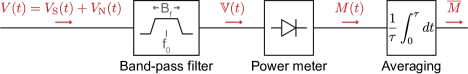
Figure S3: Model of the process for estimating power in a signal $V(t)$. A real power meter, whose response depends on the input frequency, is modelled as the combination of a band-pass-filter whose output is the filtered voltage $\mathbb{V}(t)$ followed by an ideal power meter whose output is $M(t)\equiv\mathbb{V}^{2}(t)$. The average of the meter output gives $\overline{M}$, which is the optimal estimate of ${{\langle}}\mathbb{V}^{2}{{\rangle}}$.

To do this, assume that the signal $V(t)$ whose power content we are estimating is stationary. We model the estimation process by assuming that we have a power meter whose output $M(t)$ is equal to the square of the incident voltage within its detection bandwidth:

$$M(t)\equiv\mathbb{V}^{2}(t).$$ (S93)

This may represent a real power meter, or $M(t)$ may be calculated from the digitised $V(t)$. As in Section S3.2, we must estimate the power from a record of $M(t)$ acquired over a time $\tau$. A model of this process is shown in Fig. S3.

We need the spectral density $S_{MM}[f]$. To calculate it, we first evaluate the autocorrelation function of $M(t)$. This is done with the help of Isserlis’ theorem , which states that

$$\langle M(t)M(t^{\prime})\rangle \equiv\langle\mathbb{V}^{2}(t)\mathbb{V}^{2}(t^{\prime})\rangle$$ (S100)

$$=\langle\mathbb{V}^{2}(t)\rangle\langle\mathbb{V}^{2}(t^{\prime})\rangle+2\,\langle\mathbb{V}(t)\mathbb{V}(t^{\prime})\rangle^{2}$$ (S101)

$$=\langle\mathbb{V}^{2}(0)\rangle^{2}+2\,\langle\mathbb{V}(0)\mathbb{V}(t-t^{\prime})\rangle^{2}.$$ (S102)

The theorem holds provided that $\mathbb{V}(t)$ obeys a multivariate normal distribution, which it should do because it is a sum of many independent contributions to the noise. Using Eq. (S102) in combination wih the Wiener-Khinchin theorem (Eq. (S8)) gives

$$S_{MM}[f]=2\left\{\langle\mathbb{V}^{2}(0)\rangle^{2}\delta[f]+2\int_{-\infty}^{\infty}dt\,e^{-2\pi ift}\langle\mathbb{V}(0)\mathbb{V}(t)\rangle^{2}\right\}.$$ (S103)

To evaluate the second term we again use the Wiener-Khinchin theorem, this time for the correlator $\langle\mathbb{V}(0)\mathbb{V}(t)\rangle$:

$$\int_{-\infty}^{\infty}dt\,e^{-2\pi ift}\langle\mathbb{V}(0)\mathbb{V}(t)\rangle^{2}$$

$$=\frac{1}{4}\iiint_{-\infty}^{\infty}dt\ df_{1}\ df_{2}\ S_{\mathbb{V}\mathbb{V}}[f_{1}]S_{\mathbb{V}\mathbb{V}}[f_{2}]e^{2\pi i(f_{1}+f_{2}-f)t}$$ (S104)

$$=\frac{1}{4}\iint_{-\infty}^{\infty}df_{1}\ df_{2}\ S_{\mathbb{V}\mathbb{V}}[f_{1}]S_{\mathbb{V}\mathbb{V}}[f_{2}]\delta[f_{1}+f_{2}-f]$$ (S105)

$$=\frac{1}{4}\int_{-\infty}^{\infty}df_{1}\ S_{\mathbb{V}\mathbb{V}}[f_{1}]S_{\mathbb{V}\mathbb{V}}[f_{1}-f].$$ (S106)

We now make the approximation that $f$ is small enough that $S_{\mathbb{V}\mathbb{V}}[f_{1}-f]\approx S_{\mathbb{V}\mathbb{V}}[f_{1}]$. This is valid because in the final evaluation of the uncertainty, which comes from an equation analogous to Eq. (S55), the noise spectral density is multiplied by the Fourier transform of the weighting function corresponding to the final averaging step in Fig. S3. By choosing a weighting function that varies slowly (e.g. by averaging over a long time $\tau$), we suppress high-frequency components of $W[f]$. Applying this approximation to Eq. (S106) and substituting into Eq. (S103) gives

$$S_{MM}[f]\approx 2\langle\mathbb{V}^{2}(0)\rangle^{2}\delta[f]+\int_{-\infty}^{\infty}df_{1}\,S_{\mathbb{V}\mathbb{V}}^{2}[f_{1}].$$ (S107)

The first term, which is proportional to the average power, contains the signal; the second term is the noise $S_{MM}^{\mathrm{N}}[f]$.

We now use analogs of Eqs. (S42) and (S57) to calculate the expectation value and variance of $\overline{M}$. For simplicity, assume that the expected power is independent of time so that the appropriate weighting function is Eq. (S39). This leads (via Eq. (S42)) to:

$$\langle\overline{M}\rangle =\langle\mathbb{V}^{2}(0)\rangle$$ (S108)

$$=\frac{1}{2}\int_{-\infty}^{\infty}S_{\mathbb{V}\mathbb{V}}[f]\,df$$ (S109)

$$=\int_{0}^{\infty}|F[f]|^{2}S_{VV}[f]\,df$$ (S110)

and (via Eq. (S57)) to:

$$\mathrm{var}(\overline{M}) =\frac{1}{2\tau}\,\lim_{f\rightarrow 0}S_{MM}^{\mathrm{N}}[f]$$ (S111)

$$=\frac{1}{\tau}\int_{0}^{\infty}|F[f]|^{4}S_{VV}^{2}[f]\,df,$$ (S112)

where $F[f]$ is the amplitude transmission of the filter before the power meter. Obviously the power estimate is related to $\overline{M}$ by

$$\overline{P}=\frac{\overline{M}}{Z_{\mathrm{0}}}.$$ (S113)

Let us approximate that $S_{VV}[f]$ is white, i.e. independent of frequency within the detection bandwidth, and that the filter transmits either all the signal or none of it. In that case Eqs. (S110) and (S112) combine into a single expression for the signal-to-noise ratio:

$$\frac{\sqrt{\mathrm{var}(\overline{M})}}{\overline{M}}\approx\frac{1}{\sqrt{\tau B_{f}}}.$$ (S114)

where $B_{f}$ is the detection bandwidth. Equation (S114) holds for any observable proportional to the power. Another way to express Eq. (S114) is as an uncertainty in estimating the spectral density, once the noise is fully characterised:

$$\sqrt{\mathrm{var}(S_{VV}^{\mathrm{S}}[f_{0}])}=\frac{S_{VV}^{\mathrm{S}}[f_{0}]+S_{VV}^{\mathrm{N}}[f_{0}]}{\sqrt{\tau B_{f}}},$$ (S115)

where $f_{0}$ is the center of the power meter’s detection bandwidth. This is the famous radiometer equation, derived by Dicke [Dicke1946] for microwave thermometers.

Another form of the radiometer equation, useful for dark-matter searches [Asztalos2010], is as the amplitude signal-to-noise ratio in the power meter’s output when it is fed a weak narrowband signal, for which $S_{VV}^{\mathrm{S}}\ll S_{VV}^{\mathrm{N}}$. Then

$$\frac{\mathrm{Signal}}{\mathrm{Noise}} \equiv\frac{\overline{M}-\langle\mathbb{V}_{\mathrm{N}}^{2}\rangle}{\sqrt{\mathrm{var}(\overline{M})}}$$ (S116)

$$=\frac{V_{\mathrm{S}}^{2}}{S_{VV}^{\mathrm{N}}\sqrt{B_{f}/\tau}}$$ (S117)

$$=\frac{P_{\mathrm{S}}}{k_{\mathrm{B}}T_{\mathrm{N}}}\sqrt{\frac{\tau}{B_{f}}},$$ (S118)

where $P_{\mathrm{S}}\equiv V_{\mathrm{S}}^{2}/Z_{\mathrm{0}}$ is the signal power. This is the signal-to-noise ratio with which a signal power $P_{\mathrm{S}}$ can be measured within an acquisition time $\tau$.

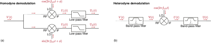
Figure S4: Circuits for generating demodulated filtered voltages. (a) Homodyne circuit, to generate voltages as in Eqs. (S125-S126). (b) Heterodyne circuit, to generate a voltage as in Eq. (S137).

S3.3 Effect of demodulation on the spectral density

As shown in Fig. 2, a high-frequency measurement nearly always involves demodulation of the signal by mixing it with a local oscillator. As one would expect, when done properly this does not affect the accuracy of any measurement based on this signal. We will now justify this statement by calculating the signal and noise spectral density after demodulation.

Suppose we have a voltage of the form

$$V(t)=A(t)\cos(2\pi f_{\mathrm{c}}t)+B(t)\sin(2\pi f_{\mathrm{c}}t)+V_{\mathrm{N}}(t),$$ (S119)

where $f_{\mathrm{c}}$ is the carrier frequency and $V_{\mathrm{N}}(t)$ is stationary noise. We want to estimate the two slowly varying quadratures $A(t)$ and $B(t)$, assumed for simplicity to be uncorrelated. An example of a voltage described by Eq. (S119) is the reflected signal from a coherently illuminated circuit when both the real and imaginary parts of the reflection coefficient are changing.

In principle we can estimate $A(t)$ and $B(t)$ directly from $V(t)$. If our measurement duration $\tau$ is longer than $1/f_{\mathrm{c}}$ but shorter than the timescale over which $A$ and $B$ vary, then by Eq. (S66) the uncertainties are

$$\sigma(A)=\sigma(B) =\sqrt{\mathrm{var}(\overline{A})}$$ (S120)

$$=\sqrt{\frac{S_{VV}^{\mathrm{N}}[f_{\mathrm{c}}]}{\tau}}$$ (S121)

provided that $S_{VV}^{\mathrm{N}}[f]$ varies smoothly near $f_{\mathrm{c}}$.

If our measurement includes a demodulation step, then we must estimate $A(t)$ and $B(t)$ from the demodulated voltage. Whether the demodulation is homodyne (with $f_{\mathrm{LO}}=f_{\mathrm{c}}$) or heterodyne (with $f_{\mathrm{LO}}\neq f_{\mathrm{c}}$), the estimates should have the same uncertainty as Eq. (S121).

S3.3.1 Homodyne demodulation

In a homodyne setup (Fig. S4(a)), we need to demodulate with two quadratures in order to extract both $A(t)$ and $B(t)$. This generates the two output voltages

$$U_{1}(t) \equiv V(t)\cos(2\pi f_{\mathrm{LO}}t)$$ (S122)

$$U_{2}(t) \equiv V(t)\sin(2\pi f_{\mathrm{LO}}t)$$ (S123)

where $f_{\mathrm{LO}}$ is the local oscillator frequency. (For simplicity we have omitted a prefactor $\sqrt{2/L_{\mathrm{C}}}$, where $L_{\mathrm{C}}$ is the mixer conversion loss .) Application of Eq. (S24) shows that the noise spectral density in both mixer outputs is related to the noise spectral density in $V(t)$ by

$$S_{UU}^{\mathrm{N}}[f]=\frac{1}{4}(S_{VV}^{\mathrm{N}}[f-f_{\mathrm{LO}}]+S_{VV}^{\mathrm{N}}[f+f_{\mathrm{LO}}]).$$ (S124)

This is illustrated in Fig. S5.

To extract $A(t)$ and $B(t)$, the demodulated voltages $U_{1}(t)$ and $U_{2}(t)$ are low-pass filtered to generate voltages $\mathbb{U}_{1}(t)$ and $\mathbb{U}_{2}(t)$. The filter cut-off should be chosen to pass all components of $A(t)$ and $B(t)$ but reject components near $2f_{\mathrm{c}}$. It then follows from Eqs. (S119) and (S122-S123) that the filtered demodulated voltages are

$$\mathbb{U}_{1}(t) =\frac{A(t)}{2}+\mathbb{U}_{1}^{\mathrm{N}}(t)$$ (S125)

$$\mathbb{U}_{2}(t) =\frac{B(t)}{2}+\mathbb{U}_{2}^{\mathrm{N}}(t),$$ (S126)

showing as expected that the outputs of the homodyne circuit contain the two signal quadratures of $V(t)$, plus noise.

The spectral density of both noise components $\mathbb{U}_{1}^{\mathrm{N}}(t)$ and $\mathbb{U}_{2}^{\mathrm{N}}(t)$ is

$$S_{\mathbb{U}\mathbb{U}}^{\mathrm{N}}[f]=\frac{1}{2}S_{VV}^{\mathrm{N}}[f+f_{\mathrm{c}}].$$ (S127)

Since $\mathbb{U}_{1,2}^{\mathrm{N}}(t)$ is stationary , we can apply Eq. (S62), obtaining

$$\sigma(A)=\sigma(B) =\sqrt{\mathrm{var}(\overline{A})}$$ (S133)

$$=\sqrt{\frac{2S_{\mathbb{U}\mathbb{U}}^{\mathrm{N}}[0]}{\tau}}$$ (S134)

$$=\sqrt{\frac{S_{VV}^{\mathrm{N}}[f_{\mathrm{c}}]}{\tau}},$$ (S135)

in agreement with Eq. (S121). This confirms that the same information is present in the homodyne outputs as was contained in the input.

Another way to express this result is to say that the sensitivity when measuring the demodulated filtered noise voltage (defined above Eq. (140)) is related to the sensitivity when measuring the voltage at the mixer input by

$$\sqrt{S_{\mathbb{U}\mathbb{U}}^{\mathrm{N}}[0]}=\sqrt{\frac{S_{VV}^{\mathrm{N}}f_{\mathrm{c}}]}{2}}$$ (S136)

but that this does not degrade the accuracy of the measurement because the signal power in each quadrature is decreased by a factor 2.

S3.3.2 Heterodyne demodulation

In a heterodyne setup (Fig. S4(b)) the entire signal information is contained in the output of a single mixer. We find

$$\mathbb{U}(t)=\frac{A(t)}{2}\cos(2\pi f_{-}t)+\frac{B(t)}{2}\sin(2\pi f_{-}t)+\mathbb{U}_{\mathrm{N}}(t)$$ (S137)

with $\mathbb{U}_{\mathrm{N}}(t)$ described by the spectral density

$$S_{\mathbb{U}\mathbb{U}}^{\mathrm{N}}[f_{-}]=\frac{1}{4}S_{VV}^{\mathrm{N}}[f_{\mathrm{c}}]$$ (S138)

where $f_{-}\equiv f_{\mathrm{c}}-f_{\mathrm{LO}}$. Once again, this leads to the measurement uncertainties given by Eq. (S121), thus confirming that heterodyne demodulation, like homodyne demodulation, preserves the information in the original signal.

S3.4 The sideband method of determining measurement sensitivity; derivation of Equation (124)

The sensitivity of a reflectometry measurement can in principle be determined from Eq. (136). However, this requires knowledge of the proportionality constant $\left|\frac{\partial V}{\partial X}\right|$, which depends on many details of the circuit. It is usually better to use Eq. (124), which we will now derive.

Figure S5: The effect of homodyne demodulation on the spectral density. (a) Cartoon of the spectral density at the mixer rf input. The signal is concentrated near frequency $f_{\mathrm{c}}$; the noise is white. (b) Cartoon of the spectral density at one of the outputs, before and after low-pass filtering.

Suppose we want to find the sensitivity to charge $Q$ on an SET. We modulate this charge in a known way, so that

$$Q(t)=\sqrt{2}\,\Delta q_{\mathrm{rms}}\cos(2\pi f_{\mathrm{M}}t),$$ (S139)

where $f_{\mathrm{M}}\ll f_{\mathrm{c}}$ is the modulation frequency and $\Delta q_{\mathrm{rms}}$ is the rms modulation amplitude. Since the reflected signal is

$$V_{\mathrm{S}}(t)=V_{\mathrm{c}}\,\mathrm{Re}\left(e^{i(2\pi f_{\mathrm{c}}t+\varphi_{\mathrm{c}})}\Gamma(t)\right),$$ (S140)

where $V_{\mathrm{c}}$ and $\varphi_{\mathrm{c}}$ are the amplitude and phase of the carrier, and since for weak modulation we have

$$\Gamma(t)=\Gamma_{0}+\frac{\partial\Gamma}{\partial Q}Q(t),$$ (S141)

this leads to

$$\begin{split}V_{\mathrm{S}}(t)&=V_{\mathrm{c}}\,\mathrm{Re}\left(\Gamma_{0}\,e^{i(2\pi f_{\mathrm{c}}t+\varphi_{\mathrm{c}})}\right)\\ &\qquad+V_{\mathrm{c}}Q(t)\,\mathrm{Re}\left(\frac{\partial\Gamma}{\partial Q}\,e^{i(2\pi f_{\mathrm{c}}t+\varphi_{\mathrm{c}})}\right).\end{split}$$ (S142)

Without loss of generality we assume $\Gamma_{0}=0$ and choose $\varphi_{\mathrm{c}}=-\mathrm{arg}\left(\frac{\partial\Gamma}{\partial Q}\right)$. The signal voltage is then

$$V_{\mathrm{S}}(t)=V_{\mathrm{c}}\left|\frac{\partial\Gamma}{\partial Q}\right|Q(t)\cos(2\pi f_{\mathrm{c}}t).$$ (S143)

We cannot yet use Eq. (136) because the $\cos(2\pi f_{\mathrm{c}}t)$ term makes $\partial V_{\mathrm{S}}/\partial Q$ non-constant. However, we can define

$$\mathbb{U}(t) \equiv\mathsf{LPF}\left\{V(t)\cos(2\pi f_{\mathrm{c}}t)\right\}$$ (S144)

$$=\frac{V_{\mathrm{c}}}{2}\left|\frac{\partial\Gamma}{\partial Q}\right|Q(t)$$ (S145)

where $\mathsf{LPF}\{\cdot\}$ denotes a low-pass filter. This gives us the proportionality we need to use Eq. (136), which leads to:

$$S_{QQ}^{\mathrm{N}}[f] =\frac{4}{V_{\mathrm{c}}^{2}|\partial\Gamma/\partial Q|^{2}}{S_{\mathbb{U}\mathbb{U}}^{\mathrm{N}}}[f]$$ (S146)

$$=\frac{2}{V_{\mathrm{c}}^{2}|\partial\Gamma/\partial Q|^{2}}S_{VV}^{\mathrm{N}}[f+f_{\mathrm{c}}]$$ (S147)

where the second line follows from Eq. (S127).

We now substitute Eq. (S139) into Eq. (S143), leading to

$$V_{\mathrm{S}}(t)=\frac{V_{\mathrm{c}}\Delta q_{\mathrm{rms}}}{\sqrt{2}}\left|\frac{\partial\Gamma}{\partial Q}\right|(\cos(2\pi f_{+}t)+\cos(2\pi f_{-}t)),$$ (S148)

where now $f_{\pm}\equiv f_{\mathrm{c}}\pm f_{\mathrm{M}}$. The corresponding spectral density is

$$S_{VV}^{\mathrm{S}}[f]=\frac{V_{\mathrm{c}}^{2}\Delta q_{\mathrm{rms}}^{2}}{4}\left|\frac{\partial\Gamma}{\partial Q}\right|^{2}(\delta[f-f_{+}]+\delta[f-f_{-}]).$$ (S149)

This describes the sidebands that appear in a spectrum such as Fig. 22(c).

Now we are ready to derive Eq. (124). First, we note that since a spectral analyser obviously cannot resolve a delta function but instead measures the average of $S_{VV}[f]$ over the resolution bandwidth $\Delta_{f}$, the apparent spectral density of the signal at the peak of a sideband is

$$s_{VV}^{\mathrm{S}}[f_{\pm}]=\frac{V_{\mathrm{c}}^{2}\Delta q_{\mathrm{rms}}^{2}}{4\Delta_{f}}\left|\frac{\partial\Gamma}{\partial Q}\right|^{2}.$$ (S150)

We then use this apparent spectral density to calculate the power SNR, with the noise spectral density taken from Eq. (S147):

$$\mathrm{SNR} \equiv\frac{s_{VV}^{\mathrm{S}}[f_{\pm}]}{S_{VV}^{\mathrm{N}}[f_{\pm}]}$$ (S151)

$$=\frac{\Delta q_{\mathrm{rms}}^{2}}{2\Delta_{f}\,S_{QQ}^{\mathrm{N}}[f_{\mathrm{m}}]},$$ (S152)

which by further rearrangement gives the charge sensitivity

$$\sqrt{S_{QQ}^{\mathrm{N}}[f_{\mathrm{m}}]}=\frac{\Delta q_{\mathrm{rms}}}{\sqrt{2\Delta_{f}\cdot\mathrm{SNR}}}.$$ (S153)

All scaling factors, such as $|\partial\Gamma/\partial Q|$, have dropped out of this equation, meaning that it can be used without knowing details of the reflectometry chain.

The final step is to re-express SNR in dB, after which Eq. (S153) becomes

$$\sqrt{S_{QQ}^{\mathrm{N}}[f_{\mathrm{m}}]}=\frac{\Delta q_{\mathrm{rms}}}{\sqrt{2\Delta_{f}}\,10^{\mathrm{SNR_{dB}}/20}}.$$ (S154)

This is Eq. (124). Clearly it can be applied to any other measured quantity instead of charge $Q$.

Conveniently, $\mathrm{SNR_{dB}}$ can be read off as a peak height as in Fig. 22(c), provided that it is large enough; if not, then the peak height overestimates $\mathrm{SNR_{dB}}$ because it fails to account for the contribution of the noise to the total sideband power.

Finally we comment on the relationship between sensitivity measured in the frequency domain (Eq. (124)) and in the time domain (Eq. (126)). If all relevant noise sources are white and no additional noise is introduced by demodulating or digitising the signal, then these two equations will give the same result. In practice, the frequency-domain method often gives a slightly better apparent sensitivity because $f_{\mathrm{m}}$ can be chosen away from noise spurs. When the target signal is nearly monochromatic, the frequency-domain method is often appropriate; for broadband signals such as for qubit readout, the frequency-domain result can be used as a lower bound but the time-domain result is usually more representative. Ultimately it is Eq. (S57) that determines which components of the noise corrupt a measurement.

S4 Charge detection table

Paper	Technique	System	$f_{\mathrm{r}}$	$Q_{\mathrm{r}}$	$\sqrt{S_{QQ}^{\mathrm{N}}}$	$\tau_{\mathrm{min}}$	$\mathcal{F}$ ($\tau_{\mathrm{int}}$)	Special features
Schoelkopf 1998 [Schoelkopf1998]	Resistive	SET Al/AlOx	1700	6	12
Fujusawa 2000 [fujisawa2000_transmission]	Resistive	SET GaAs	680	10	500			No cryo amp.
Fujusawa 2000 [Hirayama2000]	Resistive	SET GaAs	700	4	36
Aassime 2001 [Delsing2001]	Resistive	SET Al/AlOx	331	18	6.3
Aassime 2001 [Schoelkopf2001]	Resistive	SET Al/AlOx	332	24	3.2
Lehnert 2003 [Schoelkopf2003]	Resistive	SET Al/AlOx	500	10	40
Lu 2003 [Rimberg2003]	Resistive	SET Al/AlOx	1091		24
Roschier 2004 [Schoelkopf2004]	Resistive	SET Al/AlOx	471.2		38
Brenning 2006 [Delsing2006]	Resistive	SET Al/AlOx	345	11	0.9
Angus 2007 [Clark2007]	Resistive	SET Si	340	20	7.2
Ares 2016[Laird2016matching]	Resistive	SET GaAs	211		1650
Schupp 2020[Schupp2020]	Resistive	SET GaAs	200	15	60			SQUID amp.
Qin 2006 [Williams2006]	QPC CS	DQD GaAs	810	10	2000
Cassidy 2007 [Smith2007]	QPC CS	DQD GaAs	332	8	200
Reilly 2007 [Gossard2007]	QPC CS	DQD GaAs	220	15	1000
Barthel 2009 [Gossard2009]	QPC CS	DQD GaAs			600		90 (6 $\upmu$s)
Mason 2010 [Kycia2010]	QPC CS	DQD GaAs	763		146			Superconducting $L_{\mathrm{C}}$
House 2016 [Simmons2016]	SET CS	DQD Si:P	283.6	45		55 ns
Volk 2019 [Kuemmeth2019]	SET CS	DQD Si/SiGe	136		1500	2.1 $\upmu s$
Keith 2019 [Simmons2019SingleShot]	SET CS	DQD Si:P	223	40	50		97 (1.5 $\upmu$s)
Noiri 2020 [Tarucha2020]	SET CS	DQD Si	206.7			22 ns*	99.99 (1.8 $\upmu$s)
Connors 2020 [Nichol2020]	SET CS	DQD SiGe					99.9 (1 $\upmu$s )
Petersson 2010 [Petersson2010]	Disp.	DQD GaAs	385	8	200
Stehlik 2015 [Petta2015]	Disp.	DQD InAs NW	7881	3000		7 ns		QED cavit, JPA
Colless 2013 [Reilly2013]	Disp.	DQD GaAs	704	70	6300	5 $\upmu$s
Gonzalez 2015 [Gonzalez-Zalba2015_limits]	Disp.	DQD Si	335	42	37
Pakkiam 2018 [Simmons2018]	Disp.	DQD Si	339.6	266			82.3 (300 $\upmu$s)	Superconducting $L_{\mathrm{C}}$
Ahmed 2018 [Gonzalez-Zalba2018_rfgate]	Disp.	DQD Si	616	790	1.3			Superconducting $L_{\mathrm{C}}$
West 2019 [Dzurak2019]	Disp.	DQD Si	266.9	38		2.6 ms	73 (2 ms)
Schaal 2019 [Morton2020_JPA]	Disp.	DQD Si	621.9	966		80 ns		Superconducting $L_{\mathrm{C}}$, JPA
Zheng 2019 [Vandersypen2019]	Disp.	DQD Si	5711.6	2600	400	170 ns	98 (6 $\upmu$s)	QED cavity
Ibberson 2021 [Gonzalez-Zalba2021Interaction]	Disp.	DQD Si	1880		100	10 ns		Superconducting $L_{\mathrm{C}}$, waveguide
House 2016 [Simmons2016]	Disp. CS	DQD Si:P	244.8	100		550 ns
Urdampilleta 2019 [Urdampilleta2019]	Disp. CS	DQD Si		234	58		99 (1 ms)
Schaal 2019 [Morton2020_JPA]	Disp. CS	DQD Si	621.9	966	0.25			Superconducting $L_{\mathrm{C}}$, JPA
Bohuslavsky 2020 [Kuemmeth2020quadruple]	Disp. CS	DQD Si	191			17 $\upmu s$*
Chanrion 2020 [Urdampilleta2020]	Disp. CS	DQD Si	286	70	2100

Table SI: Table referencing the sensitivity $\sqrt{S_{QQ}^{\mathrm{N}}}$ (in $\upmu e/\sqrt{\mathrm{Hz}}$), from available sources, over reading the charge occupation of single electron transistors (SETs) or double quantum dots (DQDs) of various sorts. In the SET experiments, $\sqrt{S_{QQ}^{\mathrm{N}}}$ refers to measuring the charge occupation of the SET itself which are obtain by detecting its variation of resistance with the rf setup (Resistive). In the DQD experiments, $\sqrt{S_{QQ}^{\mathrm{N}}}$ refer to measuring the charge occupation of the two quantum dots using either a radio-frequency charge sensor a quantum point contact charge sensor (QPC CS), a SET charge sensor (SET CS), in-situ dispersive readout (Disp.) or dispersive charge sensing (Disp. CS). Next to the charge sensitivity $\sqrt{S_{QQ}^{\mathrm{N}}}$ and the minimum integration time $\tau_{\mathrm{min}}$ to reach $\text{SNR}=1$, we display the resonance frequency $f_{\mathrm{r}}$ (in MHz), the total quality factor $Q_{\mathrm{r}}$ and in the case of single shot readout of spin qubit: the fidelity (in %) $\mathcal{F}$ (and corresponding integration time $\tau_{\mathrm{int}}$). The last column contain special features of the resonators or the setups.
* These papers do not report $\tau_{\mathrm{min}}$ directly; instead they report the SNR at another value of $\tau_{\mathrm{int}}$, and we assume $\tau_{\mathrm{min}}=\tau_{\mathrm{int}}^{2}/\text{SNR}_{x}^{2}$.

S5 Component table

	Name	Reference
Resistor
1 k$\Omega$	TE RP73D1J1K0BTDG	Gonzalez-Zalba2019tunable
10 k$\Omega$	TE RP73D1J10KBTDG	Gonzalez-Zalba2019tunable
10 k$\Omega$	ERA3APB103V
100 k$\Omega$	TE RP73D1J100KBTDG	Gonzalez-Zalba2019tunable 6=1
Capacitor    7=2
1 pF	KEMET BR06C109BAGAC	Gonzalez-Zalba2019tunable
100 pF	Murata GRM1885C1H101JA01	Gonzalez-Zalba2019tunable
100 pF	CC0603JRNPO9BN101
1 nF	Murata GRM1885C1H102JA01	Gonzalez-Zalba2019tunable
10 nF	KEMET C0603C103J3GACTU	Gonzalez-Zalba2019tunable
10 nF	TDK CGA3E2C0G1H103J080AA	13=1
Inductor    14=2
270 nH	TDK B82498F3271J001	Gonzalez-Zalba2019tunable
390 nH	EPCOS B82498B3391J
470 nH	B82498B3471J
560 nH	TDK B82498F3561J001	Gonzalez-Zalba2019tunable
820 nH	Coilcraft 1206CS-821XJL	Kuemmeth2020quadruple
820 nH	Coilcraft 1206CS-821XJE	Simmons2018
1200 nH	Coilcraft 1206CS122XJEB	Kuemmeth2019
Varicap diode
0.7 pF	MA46H200	Gonzalez-Zalba2019tunable
11 pF	MACOM MA46H204-1056	Laird2016matching, Simmons2016, Gonzalez-Zalba2019tunable

Table SII: List of components for PCB board resonator used in various experiments. PCB sample holders stuffed with SMD inductors for reflectometry are also commercially available from QDevil (www.qdevil.com).

Bibliography