Breather modes of fully nonlinear mass-in-mass chains

Abstract

We propose a model for a chain of particles coupled by nonlinear springs in which each mass has an internal mass and all interactions are assumed to be nonlinear. We show how to construct an asymptotic solution of this system using multiple timescales, the systematic solution of coupled equations by repeated application of a consistency condition. Our results show that for some combinations of nonlinearity the dynamics are governed by the NLS as in the more usual mass-in-mass chains with linear interactions between inner and outer masses. However, when both nonlinearities have quadratic components, we show that the asymptotic reduction results in a Ginzburg-Landau equation instead of NLS.

I Introduction

The dynamics exhibited by chains of particles coupled by nonlinear springs has been of long-term interest since the pioneering study of Fermi, Pasta, Ulam and Tsingou (FPUT) fpu . Initially, travelling waves were the main focus of interest zk ; fw ; however, for the last couple of decades, the behaviour of breather-modes in these systems has been a key component ma ; chong , and more recently, the types of chain which exihibit these mode has been extended, to diatomic chains cretegny ; livi ; jw-diFPU , two-dimensional lattices flach ; jce+marin ; jce+marin2 ; dario2 ; bajars ; butt ; butt2 ; alz , and mass-in-mass chains. For a recent review of the applications of these systems, see Archilla et al. QinMica .

In mass-in-mass systems, the interconnected nodes are assumed to contain an internal oscillator, which allows a more complicated frequency response. Most commonly, the along-chain interactions are assumed to be nonlinear, whilst the interactions between inner and outer particles are linear as in dario3 ; ksx ; vain ; however, in some cases, the along chain interactions are linear, and the inner-outer interactions are nonlinear, for example, see Wallen et al. wallen . Liu et al. vain investigate the lifetimes of bright breathers in the problem with Hertzian contact by reducing the equations to a discrete $p$-Schrodinger equation. Liu et al. liu use Schrodinger reductions to investigate the form and stability of localised energy transport in these systems, they note the existence of both bright and dark breathers in alternating regions of parameter space. Conditions for the existence of travelling waves have been explored by Kevrekidis et al. ksx . In dario3 , Kevrekidis et al. analyse energy trapping due to a localised defect in a Hertzian chain with internal masses. Bonanomi et al. bona also analyse wave propagation in chains with internal resonators; they observe a wide gap between the frequency bands corresponding to linear waves. The simpler case of a single resonant defect is considered by Lydon et al lydon .

In this paper we consider the case where there is an internal resonator at every node along the lattice, and further generalise these mass-in-mass systems to allow both interactions to be nonlinear, that is, both between the internal oscillator and external shell, and the interaction between neighbouring particles along the chain. One application of such a model is a precompressed Hertzian chain, of particles in contact, in which each particle contains an identical nonlinear resonator. Such systems clearly have nonlinear nearest-neighbour interactions, which can be adjusted by varying the amount of precompression applied. Whilst we acknowledge that Hertzian contact may be more strongly nonlinear than an internal resonator, no experimental oscillator can be precisely linear, so it seems natural to model both internal and nearest-neighbour interactions as nonlinear. The results we derive below suggest that the effects of combining these two nonlinearities can be significant.  From a mathematical modelling perspective, the inclusion of nonlinear terms in both interaction forces is a natural generalisation by which the mass-in-mass model is extended. Much of the previous theoretical analysis of mass-in-mass systems has relied on this inner-outer relationship being linear, which leads to some simplification of the theory. In the analysis presented below, we include nonlinear terms, showing how the nonlinear terms can be accommodated in a full asymptotic solution of the dynamics using multiple scales techniques bo . We find conditions on the form of the nonlinearities required for breathers to be long-lived.

II Fully nonlinear mass in mass system

Figure 1 illustrates the chain of coupled mass-in-mass oscillators that we are modelling. We define the displacements of the outer oscillators of mass $m$ by $q_{n}(t)$, with corresponding momenta $p_{n}(t)$. These are coupled to their nearest neighbours ($n\pm 1$), as well as the inner masses ($M$), whose displacements and momenta are given by $Q_{n}(t)$, $P_{n}(t)$. We derive the equations of motion from the Hamiltonian

$$H=\sum_{n}\frac{p_{n}^{2}}{2m}+\frac{P_{n}^{2}}{2M}+V(q_{n+1}-q_{n})+W(q_{n}-Q_{n}),$$ (2.1)

where the potential energies are given by

$$V(\phi)= \;\mbox{$\frac{1}{2}$}\phi^{2}+\mbox{$\frac{1}{3}$}a\phi^{3}+\mbox{$\frac{1}{4}$}b\phi^{4},$$ (2.2)

$$W(\psi)= \;\mbox{$\frac{1}{2}$}\rho\psi^{2}+\mbox{$\frac{1}{3}$}\alpha\psi^{3}+\mbox{$\frac{1}{4}$}\beta\psi^{4},$$ (2.3)

for some $\rho>0$, with $a,b,\alpha,\beta$ of either sign.

The equations of motion are then

$$m\frac{\mbox{d}^{2}q_{n}}{\mbox{d}t^{2}}= \;V^{\prime}(q_{n+1}\!-\!q_{n})-V^{\prime}(q_{n}\!-\!q_{n-1})-W^{\prime}(q_{n}\!-\!Q_{n}),$$

(2.4)

$$M\frac{\mbox{d}^{2}Q_{n}}{\mbox{d}t^{2}}= \;W^{\prime}(q_{n}-Q_{n}),$$ (2.5)

where

$$V^{\prime}(\phi)= \;\phi+a\phi^{2}+b\phi^{3},$$ (2.6)

$$W^{\prime}(\psi)= \;\rho\psi+\alpha\psi^{2}+\beta\psi^{3},$$ (2.7)

represent the forces due to nearest-neighbour, and inner-outer interactions. We propose to investigate the form small amplitude breathers in this system, using multiple-scales asymptotic methods bo .

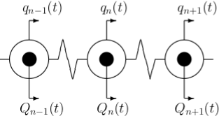
Figure 1: Illustration of the mass-in-mass chain whose dynamics are described in this paper.

III Asymptotic analysis

We seek waves which have the form of a linear wave whose amplitude is modulated by a slowly-varying envelope. We introduce a small parameter, $\epsilon$, which is proportional to the amplitude of the breather soluton; since we use a multiple scales techniques, we introduce a large space scale ($y$) and two long timescales,

$$\epsilon\ll 1,\quad y=\epsilon n,\quad\tau=\epsilon t,\quad T=\epsilon^{2}t.$$ (3.1)

The leading order linear wave has the form $q,Q\propto\mbox{Re}({\rm e}^{i\theta})=\mbox{Re}({\rm e}^{i(kn-\omega(k)t})$. Since we wish to consider quadratic nonlinearities, the centre of the oscillation may be offset from zero, so we include a ‘zero’-mode in addition to the envelope that describes the amplitude of the oscillations. We use $F_{j}(y,\tau,T),P_{j}(y,\tau,T)$ for the leading order expressions for the amplitude envelope and zero mode, hence our ansatz is

$$q_{n}(t)= \;\epsilon{\rm e}^{i\theta}F_{1}(y,\tau,T)+\epsilon F_{0}(y,\tau,T)$$

$$\;+\epsilon^{2}\left[{\rm e}^{2i\theta}G_{2}+{\rm e}^{i\theta}G_{1}+G_{0}\right]$$

$$+\epsilon^{3}\left[{\rm e}^{3i\theta}H_{3}+{\rm e}^{2i\theta}H_{2}+{\rm e}^{i\theta}H_{1}+H_{0}\right]$$

$$+\epsilon^{4}\left[I_{0}+\ldots\right]+\ldots+c.c.,$$ (3.2)

$$Q_{n}(t)= \;\epsilon{\rm e}^{i\theta}P_{1}(y,\tau,T)+\epsilon P_{0}(y,\tau,T)$$

$$\;+\epsilon^{2}\left[{\rm e}^{2i\theta}S_{2}+{\rm e}^{i\theta}S_{1}+S_{0}\right]$$

$$+\epsilon^{3}\left[{\rm e}^{3i\theta}R_{3}+{\rm e}^{2i\theta}R_{2}+{\rm e}^{i\theta}R_{1}+R_{0}\right]$$

$$+\epsilon^{4}\left[U_{0}+\ldots\right]+\ldots+c.c.,$$ (3.3)

where $G_{j},H_{j},S_{j},R_{j}$ describe the amplitudes of other modes caused by nonlinearities, which are also functions of $(y,\tau,T)$ and are determined by correction terms of higher order in $\epsilon$. These expressions are substituted into the equations of motion (2.4)–(2.5), then all terms are expanded in powers of $\epsilon$. From (3.1), the time derivative is expanded as $\mbox{d}/\mbox{d}t=\partial_{t}+\epsilon\partial_{\tau}+\epsilon^{2}\partial_{T}$. Equating terms of equal powers of $\epsilon$ and equal frequencies (in terms of ${\rm e}^{im\theta}$, for $m=0,1,2,\ldots$), gives a hierarchy of coupled pairs of equations which determine the shape of the envelopes $F_{j},P_{j},G_{j},S_{j}$, etc.; in the remainder of this section we work through the systems of equations sequentially.

III.1 Equations at $\mathcal{O}(\epsilon{\rm e}^{i\theta})$

Substituting the ansatz (3.2)–(3.3) into the governing equations (2.4)–(2.5) and expanding, we find, at leading order

$${\bf M}\begin{pmatrix}F_{1}\\ P_{1}\end{pmatrix}:= \begin{pmatrix}m\omega^{2}\!-\!4\sin^{2}\mbox{$\frac{1}{2}$}k\!-\!\rho&\rho\\ \rho&M\omega^{2}\!-\!\rho\end{pmatrix}\begin{pmatrix}F_{1}\\ P_{1}\end{pmatrix}=\begin{pmatrix}0\\ 0\end{pmatrix}.$$

For there to be nonzero solutions for $F_{1},P_{1}$, we need the matrix to be singular, which occurs when the frequency respons, $\omega$, is given by

$$\omega^{2}= \;\frac{1}{2mM}\left[\rho\,M\!+\!\rho\,m\!+\!4M\sin^{2}\mbox{$\frac{1}{2}$}k\pm\sqrt{D}\right],$$

$$D= \;(\rho\,M\!+\!\rho\,m\!+\!4M\sin^{2}\mbox{$\frac{1}{2}$}k)^{2}-16Mm\rho\,\sin^{2}\mbox{$\frac{1}{2}$}k.$$

(3.5)

This relationship is illustrated in Figure 2 for a variety of values of $\rho\,,m,M$. Note that there are two modes for each frequency (discounting the $\omega\mapsto-\omega$ symmetry). We refer to the one with the larger frequency as the optical mode ($\omega_{\mbox{\scriptsize op}}$), and the smaller frequency one as the acoustic mode ($\omega_{\mbox{\scriptsize ac}}$).

To give simple explicit examples, we consider the asymptotic cases of large mass ratios, defining

$$\mu=M/m,$$ (3.6)

as the ratio of the inner mass to the outer. The speed of sound in the lattice is defined by $c_{0}=\lim_{k\rightarrow 0}\omega_{\mbox{\scriptsize ac}}(k)/k$, which gives

$$c_{0}=\frac{1}{\sqrt{m(1+\mu)}}.$$ (3.7)

This speed is small when the mass ratio ($\mu$) is large.

To illustrate the types of behaviour that may be observed, we consider mass ratios (3.6), either side of unity, namely 3 and 0.3; and spring constants above and below unity, i.e. $\rho\,=1/3,3$. We also consider cases with no quadratic nonlinearities ($\alpha=a=0$) and with both ($\alpha\neq 0\neq a$), as well as with one but not the other (both $\alpha=0\neq a$ and $\alpha\neq 0=a$).

We observe that in many cases there are a large range of wavenumbers, $k$, which give rise to almost the same frequency ($\omega$). For example, in the lower right panel, the optical frequency is almost independent of wavenumber, whilst the acoustic mode has a strong dependence on $k$; that is, as the wavenumber $k$ varies from zero to $\pi/2$, the acoustic band covers a considerable range of frequencies, ($0\leq\omega\leq 0.53$), whereas, in the same range of $k$, only a very small range of frequencies are covered by the optical band, namely ($1.14\leq\omega\leq 1.19$ – less than one tenth of range of the acoustic band).

This is in contrast with the top left panel, where the situation is reversed: the acoustic mode is almost independent on $k$ whilst the optical mode varies significantly with $k$; here, as $k$ ranges from zero to $\pi/2$, the acoustic band spans $0\leq\omega\leq 0.32$ whilst the optical band spans $0.67\leq\omega\leq 2.08$ – about four times the range of the acoustic band. In the lower left panel, both modes vary with $k$. the acoustic and optical modes spanning $0\leq\omega\leq 0.73$ and $2.00\leq\omega\leq 2.73$ respectively. Similarly, the top right panel also has relatively wide ranges, namely $0\leq\omega\leq 0.32$ and $0.38\leq\omega\leq 0.67$. The size of the gap between the bands is also affected strongly by $\rho\,$ and $\mu$, in the four panels the gaps are 0.33, 0.06, 1.27, 0.61 –which we note are small in the first two cases–when $\rho$ is small and significantly larger when $\rho$ is larger.

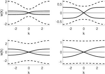
Figure 2: Illustration of the dispersion relation (3.5) for the cases: top left: $\rho=1/3$, $\mu=3$ ($m=1$, $M=3$); top right: $\rho=1/3$, $\mu=0.3$, ($m=10$, $M=3$); bottom left: $\rho=3$, $\mu=3$ ($m=1$, $M=3$); bottom right: $\rho=3$, $\mu=0.3$ ($m=10$, $M=3$). The solid lines correspond to the acoustic mode and the dashed lines to the optical. These cases and key apply to the illustrations in all later figures.

From Figure 2 we also note that there is a gap between the acoustic and optical modes, and this gap can be relatively wide (as in the bottom panels), but also may be very small (top right panel). It is the regions above the optical mode, and between the acoustic and optical modes that we expect breathers to exist and be stable. We note that the gap between the two branches is always positive, and is given by

$$\Delta\omega= \;\omega_{\mbox{\scriptsize op}}(0)-\omega_{\mbox{\scriptsize ac}}(\pi)=\frac{\omega_{\mbox{\scriptsize op}}^{2}(0)-\omega_{\mbox{\scriptsize ac}}^{2}(\pi)}{\omega_{\mbox{\scriptsize op}}(0)+\omega_{\mbox{\scriptsize ac}}(\pi)},$$ (3.8)

which is always positive, since the numerator is given by

$$\Delta^{2}= \omega_{\mbox{\scriptsize op}}^{2}(0)-\omega_{\mbox{\scriptsize ac}}^{2}(\pi)$$

$$= \frac{\rho\,}{2\mu m}\left[1+\mu-\frac{4\mu}{\rho\,}+\sqrt{\left(1+\mu-\frac{4\mu}{\rho\,}\right)^{2}+\frac{16\mu^{2}}{\rho\,}}\right].$$ (3.9)

For any given mass ratio, $\mu$, the narrowest gap is obtained when the spring constant is given by $\rho\,=4\mu/(1+\mu)$.

In the limit of small $\mu$, we find

$$\omega_{\mbox{\scriptsize ac}}^{2}\sim \;\frac{4}{m}\sin^{2}(\mbox{$\frac{1}{2}$}k)(1-\mu),\quad \omega_{\mbox{\scriptsize op}}^{2}\sim \;\frac{\rho\,(1+\mu)}{\mu m},$$ (3.10)

whilst for large mass ratio ($\mu\gg 1$) we have

$$\omega_{\mbox{\scriptsize ac}}^{2}\sim \;\frac{4\rho\,\sin^{2}(\mbox{$\frac{1}{2}$}k)}{\mu m(\rho\,+4\sin^{2}(\mbox{$\frac{1}{2}$}k))}, \omega_{\mbox{\scriptsize op}}^{2}\sim \;\frac{\rho\,+4\sin^{2}(\mbox{$\frac{1}{2}$}k)}{m}.$$

The small $\mu$ case corresponds to the inner oscillators having negligible mass, whereas in case of large $\mu$, the inner masses dominate. Whilst we might expect the former case to be a regular perturbation of the FPUT system and the latter case give rise to more exotic dynamics, the observed behaviour will also depend on the strength of the interaction between the inner and outer masses, $\rho\,$, and, at larger amplitudes, also $\alpha,\beta$.

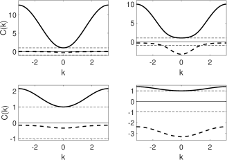
Figure 3: Illustration of the relationship between $P_{1}$ and $F_{1}$, namely $C(k)=P_{1}/F_{1}$ given by (3.12), for the cases top left: $\rho=1/3$, $\mu=3$, ($m=1$, $M=3$); top right: $\rho=1/3$, $\mu=0.3$, ($m=10$, $M=3$); bottom left: $\rho=3$, $\mu=3$, ($m=1$, $M=3$); bottom right: $\rho=3$, $\mu=0.3$, ($m=10$, $M=3$). The solid lines correspond to the acoustic mode and the dashed lines to the optical.

The solution of the matrix problem (LABEL:eq11) is given by

$$P_{1}(y,\tau,T)= \;C(k)F_{1}(y,\tau,T),$$

$$C(k)= \;\frac{\rho\,}{\rho\,-M\omega(k)^{2}}.$$ (3.12)

The dependence of $C$ on wavenumber $k$ is shown in Figure 3. Note that $C$ is real for all wavenumbers $k$. The value of $C$ differs in sign between the acoustic and optical cases. In cases where $C<0$, the inner and outer oscillators are out of phase, where as $C>0$ implies the oscillators are in-phase. We note that in the majority of cases illustrated in Figure 3, we have $|C|>1$ which indicates that the motion of the internal oscillators are larger in amplitude than the external oscillators. The in-phase (acoustic) modes always correspond to larger amplitude oscillation of the internal nodes, that is $C>1$; whereas the out-of-phase modes occur in both the regimes $C<-1$ and $-1<C<0$; the latter range corresponding to the outer oscillator having a larger amplitude than the inner. Compare the lower two panels of Figure 3 which shows results for differing values of $\mu$; and note also, the top right panel, which shows both $C<-1$ and $-1<C<0$ depending on wavenumber $k$, (for the same $\mu$ and $\rho$).

The asymptotic limit cases are given by

$$C_{\mbox{\scriptsize ac}}= \;1+4\mu\sin^{2}(\mbox{$\frac{1}{2}$}k),\quad C_{\mbox{\scriptsize op}}= \;-\frac{1}{\mu},$$ (3.13)

for small $\mu$; and for large $\mu$ we have

$$C_{\mbox{\scriptsize ac}}= \;1+\frac{4}{\rho\,}\sin^{2}(\mbox{$\frac{1}{2}$}k), C_{\mbox{\scriptsize op}}= \;-\frac{\rho\,}{\mu(\rho\,+4\sin^{2}(\mbox{$\frac{1}{2}$}k))}.$$

Note that, whilst the relative amplitudes are $\mathcal{O}(1)$ in both the acoustic cases, in the optical cases, we have $-C_{\mbox{\scriptsize op}}\gg 1$ in the small $\mu$ limit, and $-C_{\mbox{\scriptsize op}}\ll 1$ in the large $\mu$ limit.

III.2 Equations at $\mathcal{O}(\epsilon{\rm e}^{0i\theta})$

Considering terms of $\mathcal{O}(\epsilon{\rm e}^{0i\theta})$, we obtain the equation $0=\rho(F_{0}-P_{0})$ from both (2.4) and (2.5). Thus we write $P_{0}=F_{0}$, where $F_{0}$ will be determined from higher order equations.

III.3 Equations at $\mathcal{O}(\epsilon^{2}{\rm e}^{0i\theta})$

At this order, we again find that both equations (2.4) and (2.5) give the same relationship between $G_{0},S_{0},F_{1},P_{1}$, namely

$$0=\rho\,(G_{0}-S_{0})+\rho\,(G_{0}^{*}-S_{0}^{*})+2\alpha|F_{1}-P_{1}|^{2}.$$ (3.15)

Hence, once $G_{0}$ is known, $S_{0}$ is given by

$$S_{0}=G_{0}+\frac{\alpha}{\rho\,}(C-1)^{2}|F_{1}|^{2}.$$ (3.16)

To determine $G_{0},S_{0}$ independently, if these were needed, we would have to consider (3.16) in conjunction with equations from the higher order, namely terms of $\mathcal{O}(\epsilon^{4}{\rm e}^{0i\theta})$ (see Sec III.7 for details).

III.4 Equations at $\mathcal{O}(\epsilon^{2}{\rm e}^{2i\theta})$

The second harmonic terms are governed by

$$\begin{pmatrix}4m\omega^{2}\!-\!4\sin^{2}k\!-\!\rho&\rho\\ \rho&4M\omega^{2}\!-\!\rho\end{pmatrix}\begin{pmatrix}G_{2}\\ S_{2}\end{pmatrix}\qquad$$

$$\qquad=\begin{pmatrix}\alpha(F_{1}\!-\!P_{1})^{2}+16iaF_{1}^{2}\sin^{3}(\mbox{$\frac{1}{2}$}k)\cos(\mbox{$\frac{1}{2}$}k)\\ -\alpha(F_{1}\!-\!P_{1})^{2}\end{pmatrix}.$$

Hence $G_{2},S_{2}$ can be obtained from $F_{1}$, and $P_{1}=CF_{1}$ by inverting the first matrix in (LABEL:e2e2eq), which leads to

$$\begin{pmatrix}G_{2}\\ S_{2}\end{pmatrix}= \;\frac{4F_{1}^{2}}{D_{2}}\begin{pmatrix}\alpha M\omega^{2}(C\!-\!1)^{2}+4ia\varphi(M\omega^{2}\!-\!\rho\,)\\ \alpha(C\!-\!1)^{2}(\sin^{2}k\!-\!m\omega^{2})-4ia\rho\,\varphi\end{pmatrix},$$

$$D_{2}= \;(4M\omega^{2}\!-\!\rho\,)(4m\omega^{2}\!-\!4\sin^{2}k\!-\!\rho\,)-\rho\,^{2},$$

$$\varphi= \;\sin^{3}(\mbox{$\frac{1}{2}$}k)\cos(\mbox{$\frac{1}{2}$}k).$$ (3.18)

Note that both $G_{2}$ and $S_{2}$ contain both real and imaginary components, with factors of $\alpha$ and $a$ respectively. The expressions

$$G_{2}= \;(\widehat{\alpha}_{g}+i\widehat{a}_{g})F_{1}^{2},\qquad S_{2}=(\widehat{\alpha}_{s}+i\widehat{a}_{s})F_{1}^{2},$$ (3.19)

will be used in calculations at higher order, to obtain a closed expression for $F_{1}$, see Section III.8, note that $\widehat{\alpha}_{g},\widehat{a}_{g},\widehat{\alpha}_{s},\widehat{a}_{s}$ are all real.

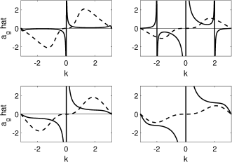
Figure 4: Illustration of the dependence of $\widehat{a}_{g}$ on wave number $k$ given by (3.18)–(3.19), for the cases top left: $\rho=1/3$, $\mu=3$, ($m=1$, $M=3$); top right: $\rho=1/3$, $\mu=0.3$, ($m=10$, $M=3$); bottom left: $\rho=3$, $\mu=3$, ($m=1$, $M=3$); bottom right: $\rho=3$, $\mu=0.3$, ($m=10$, $M=3$). The thick solid lines correspond to the acoustic mode and the dashed lines to the optical. In all panels, the optical cases (dashed-lines) are scaled up, by factors of 10,10,30,100 respectively.

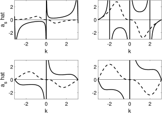
Figure 5: Illustration of the dependence of $\widehat{a}_{s}$ on wave number $k$ given by (3.18)–(3.19), for the cases top left: $\rho=1/3$, $\mu=3$, ($m=1$, $M=3$); top right: $\rho=1/3$, $\mu=0.3$, ($m=10$, $M=3$); bottom left: $\rho=3$, $\mu=3$, ($m=1$, $M=3$); bottom right: $\rho=3$, $\mu=0.3$, ($m=10$, $M=3$). The thick solid lines correspond to the acoustic mode and the dashed lines to the optical. In all panels, the optical cases (dashed-lines) are scaled up, by factors of 30,30,100,100 respectively.

Figures 4, 5, 6, 7 illustrate the amplitude of the terms $\widehat{\alpha}_{g}$, $\widehat{a}_{g}$, $\widehat{\alpha}_{s}$, $\widehat{a}_{s}$ as functions of wavenumber $k$. We note that in many cases, the limit $k\rightarrow 0$ in the acoustic case leads to a singularity. This limit corresponds to the formation of a travelling wave, rather than a breather-mode, and different asymptotic scalings are required to consider this case, further details regarding travelling waves are given in appendix A. Other singularities occur when $D_{2}=0$, these happen when the frequency $\omega$ (3.5) satisfies

$$0=4\mu(m\omega^{2})^{2}-m\omega^{2}(\rho\,+\rho\,\mu+4\mu\sin^{2}k)+\rho\,\sin^{2}(k),$$ (3.20)

which correspond to resonances between the fundamental mode and second harmonics.

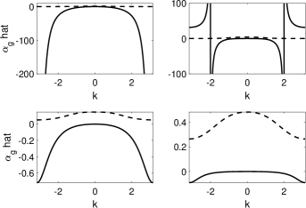
Figure 6: Illustration of the dependence of $\widehat{\alpha}_{g}$ on wave number $k$ given by (3.18)–(3.19), for the cases top left: $\rho=1/3$, $\mu=3$, ($m=1$, $M=3$); top right: $\rho=1/3$, $\mu=0.3$, ($m=10$, $M=3$); bottom left: $\rho=3$, $\mu=3$, ($m=1$, $M=3$); bottom right: $\rho=3$, $\mu=0.3$, ($m=10$, $M=3$). The thick solid lines correspond to the acoustic mode and the dashed lines to the optical.

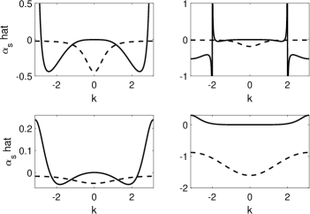
Figure 7: Illustration of the dependence of $\widehat{\alpha}_{s}$ on wave number $k$ given by (3.18)–(3.19), for the cases: top left: $\rho=1/3$, $\mu=3$, ($m=1$, $M=3$); top right: $\rho=1/3$, $\mu=0.3$, ($m=10$, $M=3$); bottom left: $\rho=3$, $\mu=3$, ($m=1$, $M=3$); bottom right: $\rho=3$, $\mu=0.3$, ($m=10$, $M=3$). The thick solid lines correspond to the acoustic mode and the dashed lines to the optical. In the top two panels, the acoustic curves are reduced in magnitude by a factor of $1/200$.

III.5 Equations at $\mathcal{O}(\epsilon^{2}{\rm e}^{i\theta})$

The final terms at $\mathcal{O}(\epsilon^{2})$ are those that have the same wavenumber and frequency as the leading order terms (${\rm e}^{i\theta}$), namely

$$\begin{pmatrix}m\omega^{2}\!-\!4\sin^{2}\mbox{$\frac{1}{2}$}k\!-\!\rho&\rho\\ \rho&M\omega^{2}\!-\!\rho\end{pmatrix}\begin{pmatrix}G_{1}\\ S_{1}\end{pmatrix}={\bf b}_{2},$$ (3.21)

$${\bf b}_{2}=\begin{pmatrix}-2i\omega mF_{1,\tau}-2iF_{1,y}\sin k\\ -2iM\omega P_{1,\tau}\end{pmatrix}.$$ (3.22)

This equation has the same matrix (${\bf M}$) on the lhs as in (LABEL:eq11), it maps all space onto the line $(\rho\,,M\omega^{2}-\rho\,)^{T}$, which is the range of ${\bf M}$. Since ${\bf M}$ is singular, there is a Fredholm consistency condition on the rhs of (3.21) which has to be satisfied in order for solutions to exist. This condition is given by ${\bf n}\cdot{\bf b}_{2}=0$, where ${\bf n}=(\rho\,-M\omega^{2},\rho\,)^{T}$ is normal to the range of ${\bf M}$.

We note that no nonlinear terms enter the equation ${\bf n}\cdot{\bf b}_{2}=0$ or the equation (3.21) for $(G_{1},S_{1})$, since the quadratic terms only generate second and zeroth harmonics, and no terms proportional to ${\rm e}^{i\theta}$.

Solving the consistency condition ${\bf n}\cdot{\bf b}_{2}=0$ using $P_{1}=CF_{1}$, we obtain

$$(\rho\,-M\omega^{2})(m\omega F_{1,\tau}+F_{1,y}\sin k)+\rho\,\omega MCF_{1,\tau}=0,$$ (3.23)

which is a first-order pde, with a travelling wave solution. We write this as $F_{1}(y,\tau,T)=F_{1}(z,T)$ where $z=y-c\tau$ and the speed $c(k)$ is given by

$$c(k)=\frac{(\rho-M\omega^{2})\sin k}{\omega[\rho\,MC\!+\!\rho\,m\!-\!Mm\omega^{2}]}=\frac{\sin k}{m\omega(1\!+\!\mu C^{2})},$$ (3.24)

the simplification being given by (3.6) and (3.12). The range of values taken by the velocity, $c$, are shown in Figure 8. Note that different values of the velocity, $c$, are obtained for the acoustic and optical cases. We note that the acoustic case is not well-defined for $k=0$, which corresponds to the case of pure travelling waves, as noted earlier and detailed in Appendix A. Both velocities are zero when the wavenumber $k=\pi$, and for optical case when $k=0$. From hereon, we work in the moving coordinate frame, taking the independent variables to be $z:=y-c(k)\tau$, and $T$.

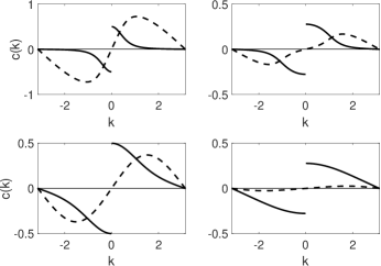
Figure 8: Illustration of the relationship between speed $c$ and wave number $k$ given by (3.24), for the cases: top left: $\rho=1/3$, $\mu=3$, ($m=1$, $M=3$); top right: $\rho=1/3$, $\mu=0.3$, ($m=10$, $M=3$); bottom left: $\rho=3$, $\mu=3$, ($m=1$, $M=3$); bottom right: $\rho=3$, $\mu=0.3$, ($m=10$, $M=3$). The solid lines correspond to the acoustic mode and the dashed lines to the optical.

In the limits of small $\mu$ we find the asymptotic limits

$$c_{\mbox{\scriptsize ac}}= \;\frac{1}{\sqrt{m}}\cos(\mbox{$\frac{1}{2}$}k)(1\!-\!\mbox{$\frac{1}{2}$}\mu),$$

$$c_{\mbox{\scriptsize op}}= \;\frac{\mu^{3/2}\sin(k)}{\sqrt{\rho\,m}}(1\!+\!\mbox{$\frac{3}{2}$}\mu),$$ (3.25)

whilst for large $\mu$, we have

$$c_{\mbox{\scriptsize ac}}= \;\sqrt{\frac{\mu}{m}}\cos(\mbox{$\frac{1}{2}$}k)\sqrt{1\!+\!\frac{4}{\rho\,}\sin^{2}(\mbox{$\frac{1}{2}$}k)}\,(1+\mathcal{O}(\mu)),$$

$$c_{\mbox{\scriptsize op}}= \;\frac{\mu\,\sin(k)}{\sqrt{m\rho\,}}\left(1\!+\!\frac{4}{\rho\,}\sin^{2}(\mbox{$\frac{1}{2}$}k)\right)^{3/2}\,(1+\mathcal{O}(\mu)).$$ (3.26)

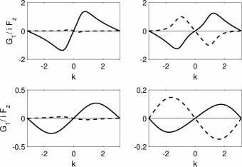
Figure 9: Illustration of the relationship between $G_{1}/iF_{1,z}$ and $k$, given by (3.29), for the cases: top left: $\rho=1/3$, $\mu=3$, ($m=1$, $M=3$); top right: $\rho=1/3$, $\mu=0.3$, ($m=10$, $M=3$); bottom left: $\rho=3$, $\mu=3$, ($m=1$, $M=3$); bottom right: $\rho=3$, $\mu=0.3$, ($m=10$, $M=3$). The solid lines correspond to the acoustic mode and the dashed lines to the optical.

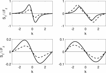
Figure 10: Illustration of the relationship between $S_{1}/iF_{1,z}$ and $k$, given by (3.29), for the cases: top left: $\rho=1/3$, $\mu=3$, ($m=1$, $M=3$); top right: $\rho=1/3$, $\mu=0.3$, ($m=10$, $M=3$); bottom left: $\rho=3$, $\mu=3$, ($m=1$, $M=3$); bottom right: $\rho=3$, $\mu=0.3$, ($m=10$, $M=3$). The solid lines correspond to the acoustic mode and the dashed lines to the optical.

As well as the speed of the envelope, we need to determine the shape of the wave, that is, find solutions for $G_{1},S_{1}$ from (3.21)–(3.22). To solve this singular system of equations, we write

$$\begin{pmatrix}G_{1}\\ S_{1}\end{pmatrix}=\widehat{G}\begin{pmatrix}\rho\,\!-\!M\omega^{2}\\ \rho\,\end{pmatrix}+\widetilde{G}\begin{pmatrix}\rho\,\\ M\omega^{2}\!-\!\rho\end{pmatrix},$$ (3.27)

in this reformulation, the unknowns $G_{1}(z,T)$, $S_{1}(z,T)$ are replaced by $\widehat{G}(z,T)$, $\widetilde{G}(z,T)$. Here, $\widehat{G}$ is the coefficient of the kernel of the singular matrix, so cannot be determined, so we assume that this is accounted for in the leading order terms $F_{1},P_{1}$, and we take $\widehat{G}=0$. This can be justified by considering the hypothetical case $\widehat{G}\neq 0$. The $\mathcal{O}({\rm e}^{i\theta})$ terms in the asymptotic series for $(q_{n},Q_{n})^{T}$ would then start

$$\begin{pmatrix}q_{n}\\ Q_{n}\end{pmatrix}\sim \;\epsilon{\rm e}^{i\theta}F_{1}\begin{pmatrix}1\\ C\end{pmatrix}+\epsilon^{2}{\rm e}^{i\theta}\widehat{G}\begin{pmatrix}1\\ C\end{pmatrix}+\epsilon^{2}{\rm e}^{i\theta}\widetilde{G}\begin{pmatrix}C\\ 1\end{pmatrix}$$

$$\;+\mathcal{O}(\epsilon^{3}{\rm e}^{i\theta}),$$ (3.28)

where $C$ is given by (3.12); note that $C\neq\pm 1$ so the vectors $(C,1)^{T}$ and $(1,C)^{T}$ are linearly independent. If we define $\widehat{F}_{1}=F_{1}+\epsilon\widehat{G}$, then $\widehat{F}_{1}$ satisfies the same equations as $F_{1}$ at leading order. Although definitions of higher order terms, $H_{1},H_{2},R_{1},R_{2}$ etc. may be modified, our expressions for $G_{0},G_{2},S_{0},S_{2},$ remain unchanged.

The last vector in (3.27) is perpendicular to the kernel, and is not in the kernel. This enables us to find $\widetilde{G}$. From the second component of (3.21)–(3.22), we find $\widetilde{G}=i\gamma_{1}F_{1,z}$ where $\gamma_{1}\in\mathbb{R}$ is given by

$$\gamma_{1}= \;\frac{2\omega cCM}{\rho\,^{2}+(M\omega^{2}-\rho\,)^{2}},$$

$$G_{1}= \;\rho\widetilde{G}=i\gamma_{1}\rho\,F_{1,z},$$

$$S_{1}= \;(M\omega^{2}-\rho\,)\widetilde{G}=i\gamma_{1}(M\omega^{2}-\rho\,)F_{1,z}.$$ (3.29)

We now have expressions for $G_{1}$, $G_{2}$, $S_{0}$, $S_{1}$, $S_{2}$ and $P_{1}$ in terms of $F_{1}$ and $G_{0}$. We need to go to higher order to find $G_{0}$ in terms of $F_{1}$ and a closed form expression for $F_{1}$.

III.6 Equations at $\mathcal{O}(\epsilon^{3}{\rm e}^{0i\theta})$

From terms of this order, we obtain the equations

$$mF_{0,\tau\tau}\!+\!mF^{*}_{0,\tau\tau}= \;F_{0,yy}+F^{*}_{0,yy}+\rho\,(R_{0}\!-\!H_{0})$$

$$+\rho\,(R_{0}^{*}\!-\!H_{0}^{*})+8a\sin^{2}(\mbox{$\frac{1}{2}$}k)(|F_{1}|^{2})_{y}$$

$$-2\alpha(F_{1}\!-\!P_{1})(G_{1}^{*}\!-\!S_{1}^{*})$$

$$-2\alpha(F_{1}^{*}\!-\!P_{1}^{*})(G_{1}\!-\!S_{1}),\;$$ (3.30)

$$\mu mP_{0,\tau\tau}+\mu mP^{*}_{0,\tau\tau}= \;\rho\,(H_{0}\!-\!R_{0})+\rho\,(H_{0}^{*}\!-\!R_{0}^{*})$$

$$+2\alpha(F_{1}\!-\!P_{1})(G_{1}^{*}\!-\!S_{1}^{*})$$

$$+2\alpha(F_{1}^{*}\!-\!P_{1}^{*})(G_{1}\!-\!S_{1}).$$ (3.31)

Noting that $P_{0}=F_{0}$, we further simplify the solution of this system by adding the two equations together, transforming to the travelling wave coordinate $z=y-c\tau$ with $c$ given by (3.24). After integrating once, we find

$$F_{0,z}=a\phi_{0}|F_{1}|^{2}=\frac{4a|F_{1}|^{2}\sin^{2}(\mbox{$\frac{1}{2}$}k)}{(1+\mu)mc^{2}-1}.$$ (3.32)

This represents the zero mode which gives the same displacements for both the inner and outer masses. The amplitude factor $\phi_{0}$ is plotted as a function of wavenumber $k$ in Figure 11.

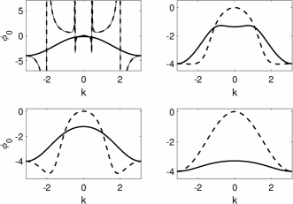
Figure 11: Illustration of $\phi_{0}$ against $k$, which determines the amplitude of the kink-shaped zero mode $F_{0}$ as given by (3.33), for the cases: top left: $\rho=1/3$, $\mu=3$, ($m=1$, $M=3$); top right: $\rho=1/3$, $\mu=0.3$, ($m=10$, $M=3$); bottom left: $\rho=3$, $\mu=3$, ($m=1$, $M=3$); bottom right: $\rho=3$, $\mu=0.3$, ($m=10$, $M=3$). The solid lines correspond to the acoustic mode and the dashed lines to the optical.

If, as frequently occurs in this type of expansion, and as will be seen in Section III.8, the equation for $F_{1}$ has the form of a nonlinear Schrodinger equation, then a typical solution has the form (3.48), which would imply $F_{0}$ is given by

$$F_{0}=\frac{4Aa\sin^{2}(\mbox{$\frac{1}{2}$}k)}{(1+\mu)mc^{2}-1}\sqrt{\frac{2D_{3}}{\eta}}\tanh\left(AZ\sqrt{\frac{\eta}{2D_{3}}}\right).$$ (3.33)

Thus we see the amplitude of the kink diverges near the speed of sound in the lattice, $c=c_{0}$, (3.7). From (3.32), we note that these divergences occur whenever the envelope wave speed $c(k)$, which is determined given by (3.24) and illustrated in Figure 8 satisfies $c(k)=c_{0}$, where $c_{0}$ is the speed of sound of the lattice given by (3.7). These divergences could be described as due to resonances with linear waves in the sonic limit.

III.7 Equations at $\mathcal{O}(\epsilon^{4}{\rm e}^{0i\theta})$

Since we need to determine $G_{0},S_{0}$ in terms of $F_{1}$ before obtaining an equation for $F_{1}$, we now consider the terms at $\mathcal{O}(\epsilon^{4}{\rm e}^{0i\theta})$ even though this is out of order. We find

$$m(G_{0,\tau\tau}\!+\!G_{0,\tau\tau}^{*})= \;G_{0,yy}+G_{0,yy}^{*}$$

$$+2ai\sin(k)(F_{1}F_{1,yy}^{*}-F_{1}^{*}F_{1,yy})$$

$$+8a\sin^{2}(\mbox{$\frac{1}{2}$}k)(F_{1}^{*}G_{1,y}+F_{1}G^{*}_{1,y})$$

$$+\rho\,(U_{0}-I_{0})+\rho\,(U_{0}^{*}-I_{0}^{*})$$

$$-2\alpha(F_{1}^{*}-P_{1}^{*})(H_{1}-R_{1})$$

$$-2\alpha(F_{1}-P_{1})(H_{1}^{*}-R_{1}^{*})$$

$$-2\alpha(G_{2}-S_{2})(G_{2}^{*}-S_{2}^{*})$$

$$-2\alpha(G_{1}-S_{1})(G_{1}^{*}-S_{1}^{*})$$

$$-2\alpha(G_{0}-S_{0})(G_{0}^{*}-S_{0}^{*})$$

$$-\alpha(G_{0}-S_{0})^{2}-\alpha(G_{0}^{*}-S_{0}^{*})^{2}$$

$$-3\beta(G_{2}-S_{2})(F_{1}^{*}-P_{1}^{*})^{2}$$

$$-3\beta(G_{2}^{*}-S_{2}^{*})(F_{1}-P_{1})^{2}$$

$$-6\beta(G_{0}-S_{0})|F_{1}-P_{1}|^{2}$$

$$-6\beta(G_{0}^{*}-S_{0}^{*})|F_{1}-P_{1}|^{2},$$ (3.34)

$$\mu m(S_{0,\tau\tau}\!+\!S_{0,\tau\tau}^{*})= \;\rho\,(I_{0}-U_{0})+\rho\,(I_{0}^{*}-U_{0}^{*})$$

$$+2\alpha(F_{1}^{*}-P_{1}^{*})(H_{1}-R_{1})$$

$$+2\alpha(F_{1}-P_{1})(H_{1}^{*}-R_{1}^{*})$$

$$+2\alpha(G_{2}-S_{2})(G_{2}^{*}-S_{2}^{*})$$

$$+2\alpha(G_{1}-S_{1})(G_{1}^{*}-S_{1}^{*})$$

$$+2\alpha(G_{0}-S_{0})(G_{0}^{*}-S_{0}^{*})$$

$$+\alpha(G_{0}-S_{0})^{2}+\alpha(G_{0}^{*}-S_{0}^{*})^{2}$$

$$+3\beta(G_{2}-S_{2})(F_{1}^{*}-P_{1}^{*})^{2}$$

$$+3\beta(G_{2}^{*}-S_{2}^{*})(F_{1}-P_{1})^{2}$$

$$+6\beta(G_{0}-S_{0})|F_{1}-P_{1}|^{2}$$

$$+6\beta(G_{0}^{*}-S_{0}^{*})|F_{1}-P_{1}|^{2}.$$ (3.35)

Adding these two equations together, and transforming to the travelling wave coordinate $z=y-c\tau$, and integrating once with respect to $z$ (and setting the constant of integration to zero), we find

$$(mc^{2}G_{0}+\mu mc^{2}S_{0}-G_{0})_{z}=$$

$$\quad ai\,\left[\sin(k)-4\gamma_{1}\rho\,\sin^{2}(\mbox{$\frac{1}{2}$}k)\right](F_{1}F^{*}_{1,z}\!-\!F_{1}^{*}F_{1,z}).$$

In the case $a=0$, this implies

$$mc^{2}G_{0}+\mu mc^{2}S_{0}-G_{0}= \;0,$$ (3.37)

which, when combined with (3.16), gives expressions for the zeroth modes $G_{0},S_{0}$ purely in terms of $F_{1}$ as

$$G_{0}= \;\gamma_{0}|F_{1}|^{2}=\frac{\alpha\mu mc^{2}(C-1)^{2}|F_{1}|^{2}}{\rho\,(1-mc^{2}-\mu mc^{2})},$$

$$S_{0}= \;\sigma_{0}|F_{1}|^{2}=\frac{\alpha(1-mc^{2})(C-1)^{2}|F_{1}|^{2}}{\rho\,(1-mc^{2}-\mu mc^{2})}.$$

(3.38)

Note that this (3.38), in together with $F_{0}$ (3.33) determines the size of the zeroth harmonics. The $F_{0}$ term depends explicitly on the along-chain quadratic parameter $a$, and determines the leading order form of the zeroth harmonic, and this component is the same for the inner and outer masses (since we have $P_{0}=F_{0}$). The $G_{0},S_{0}$ terms determine higher-order corrections, these are dependent on $\alpha$ - the coefficient of the quadratic nonlinearity of the potential controlling the difference in displacements between the inner and outer masses. Both these terms suffer singularities when $c^{2}=1/m(1+\mu)$, the speed of sound in the lattice (3.7), as was the case with $F_{0}$ (3.33). We plot the forms of $\gamma_{0},\sigma_{0}$ in Figures 12 and 13. As in Figure 11, we note that the graphs of $G_{0},S_{0}$ against $k$ exhibit several singularities. These occur in the same locations as for $\phi_{0}$ (3.32), and for the same reasons, namely that speed of the solitary wave envolope matches that of the speed of sound in the lattice, $c(k)=c_{0}$.

In the case $a\neq 0$, the solution of (LABEL:G0S0-eq3) is more complicated. Writing $F_{1}=J(z,T){\rm e}^{i\phi(z,T)}$ with $J,\phi\in\mathbb{R}$, we have

$$iF_{1}F^{*}_{1,z}\!-\!iF_{1}^{*}F_{1,z}=2J^{2}\phi_{z},$$ (3.39)

so (LABEL:G0S0-eq3) expresses a relationship between real quantitites. If an NLS equation is obtained from the $\mathcal{O}(\epsilon^{3}{\rm e}^{i\theta})$ terms, and the solution (3.48) is used for $F_{1}$, then $\phi_{z}=0$ and the solutions for $G_{0},S_{0}$ given in (3.38) remain valid. In particular, if $F_{1}=A{\rm e}^{i\Upsilon T}J(z)$, with $A,\Upsilon,J\in\mathbb{R}$, then $F_{1}F_{1,z}^{*}-F_{1}^{*}F_{1,z}=A^{2}JJ^{\prime}-A^{2}JJ^{\prime}=0$, meaning that both (3.39) and the rhs of (LABEL:G0S0-eq3) are zero, and so (3.38) still hold in the case $a\neq 0$.

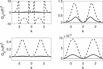
Figure 12: Illustration of the relationship between $\gamma_{0}=G_{0}/\alpha|F_{1}|^{2}$ and wave number $k$ given by (3.38), for the cases: top left: $\rho=1/3$, $\mu=3$, ($m=1$, $M=3$); top right: $\rho=1/3$, $\mu=0.3$, ($m=10$, $M=3$); bottom left: $\rho=3$, $\mu=3$, ($m=1$, $M=3$); bottom right: $\rho=3$, $\mu=0.3$, ($m=10$, $M=3$). The thick solid lines correspond to the acoustic mode and the thick dashed lines to the optical mode.

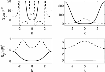
Figure 13: Illustration of the relationship between $\sigma_{0}=S_{0}/\alpha|F_{1}|^{2}$ and wave number $k$ for the cases: top left: $\rho=1/3$, $\mu=3$, ($m=1$, $M=3$); top right: $\rho=1/3$, $\mu=0.3$, ($m=10$, $M=3$); bottom left: $\rho=3$, $\mu=3$, ($m=1$, $M=3$); bottom right: $\rho=3$, $\mu=0.3$, ($m=10$, $M=3$). The thick solid lines correspond to the acoustic mode and the thick dashed lines to the optical mode. Note the wide variation in scales on the vertical axes.

In the limit of small values of $\mu=M/m$, from (3.38), we find

$$\gamma_{0,\mbox{\scriptsize ac}}(k)\sim \;\frac{4\alpha\mu^{3}\sin^{2}(k)}{\rho\,}, \gamma_{0,\mbox{\scriptsize op}}(k)\sim \;\frac{\alpha\mu^{2}\sin^{2}(k)}{\rho\,^{2}},$$

$$\sigma_{0,\mbox{\scriptsize ac}}(k)\sim \;\frac{16\alpha\mu^{2}\sin^{4}(\mbox{$\frac{1}{2}$}k)}{\rho\,}, \sigma_{0,\mbox{\scriptsize op}}(k)\sim \;\frac{\alpha}{\rho\,\mu^{2}};$$ (3.40)

whilst the large $\mu$ limit gives

$$\gamma_{0,\mbox{\scriptsize ac}}(k)\sim \;-\frac{16\alpha\sin^{4}(\mbox{$\frac{1}{2}$}k)}{\rho\,^{3}},$$

$$\gamma_{0,\mbox{\scriptsize op}}(k)\sim \;-\frac{\alpha\rho\,}{\mu^{2}(\rho\,+4\sin^{2}(\mbox{$\frac{1}{2}$}k))^{2}},$$ (3.41)

$$\sigma_{0,\mbox{\scriptsize ac}}(k)\sim \;\frac{16\alpha\sin^{4}(\mbox{$\frac{1}{2}$}k)\cos^{2}(\mbox{$\frac{1}{2}$}k)}{\mu\rho\,^{3}},\quad\sigma_{0,\mbox{\scriptsize op}}(k)\sim\;\frac{\alpha}{\mu\rho\,}.$$

From figures 12 and 13, we observe that almost all of these terms are small, the only exceptions being $\gamma_{0,\mbox{\scriptsize ac}}=\mathcal{O}(1)$ and $\sigma_{0,\mbox{\scriptsize op}}\gg 1$.

III.8 Equations at $\mathcal{O}(\epsilon^{3}{\rm e}^{i\theta})$

At this final order, we obtain a system of similar form to Section III.5, but now for $H_{1},R_{1}$, namely

$$\begin{pmatrix}m\omega^{2}\!-\!4\sin^{2}(\mbox{$\frac{1}{2}$}k)\!-\!\rho\,&\rho\,\\ \rho\,&M\omega^{2}\!-\!\rho\,\end{pmatrix}\begin{pmatrix}H_{1}\\ R_{1}\end{pmatrix}=\begin{pmatrix}b_{31}\\ b_{32}\end{pmatrix}=:{\bf b}_{3},$$ (3.42)

where

$$b_{31}= \;-2i\omega mG_{1,\tau}-2i\omega mF_{1,T}+mF_{1,\tau\tau}-2iG_{1,y}\sin k$$

$$-F_{1,yy}\cos k+2\alpha(F_{1}\!-\!P_{1})(G_{0}\!-\!S_{0}+G_{0}^{*}-S_{0}^{*})$$

$$+2\alpha(F_{1}^{*}\!-\!P_{1}^{*})(G_{2}\!-\!S_{2})+3\beta|F_{1}\!-\!P_{1}|^{2}(F_{1}\!-\!P_{1})$$

$$-32aiG_{2}F_{1}^{*}\sin^{3}(\mbox{$\frac{1}{2}$}k)\cos(\mbox{$\frac{1}{2}$}k)+48b|F_{1}|^{2}F_{1}\sin^{4}(\mbox{$\frac{1}{2}$}k)$$

$$+8aiF_{1}(F_{0,x}+F^{*}_{0,x})\sin^{2}(\mbox{$\frac{1}{2}$}k),$$

$$b_{32}= \;-2i\mu m\omega S_{1,\tau}-2i\omega\mu mP_{1,T}+\mu mP_{1,\tau\tau}$$

$$-2\alpha(F_{1}\!-\!P_{1})(G_{0}\!-\!S_{0}+G_{0}^{*}-S_{0}^{*})$$

$$-2\alpha(F_{1}^{*}\!-\!P_{1}^{*})(G_{2}\!-\!S_{2})-3\beta|F_{1}\!-\!P_{1}|^{2}(F_{1}\!-\!P_{1}).$$

(3.43)

We do not need to solve for $H_{1},R_{1}$, we only require the consistency condition on the rhs for the existence of solutions, namely ${\bf b}_{3}\cdot{\bf n}=0$, where ${\bf n}=(1,1+\mu m\omega^{2}/(\rho\,-\mu m\omega^{2}))^{T}$, which is equivalent to the definition given after (3.22).

Together with $P_{1}=CF_{1}$, and the solutions for $F_{0}$, $G_{0}$, $S_{0}$, $G_{2}$, $S_{2}$, $G_{1}$, $S_{1}$, given by (3.32), (3.12), (3.38), (3.18), (3.27), (3.29), these imply

$$i\Omega F_{1,T}= \;D_{3}F_{1,zz}+(\eta+i\zeta)|F_{1}|^{2}F_{1},$$ (3.44)

where

$$\Omega= \;-\frac{2m\omega(\rho\,+\mu\rho\,C-\mu m\omega^{2})}{(\rho\,-\mu m\omega^{2})},$$

$$D_{3}= \;\frac{\mu^{2}m^{2}\omega^{2}c^{2}C}{(\rho\,-\mu m\omega^{2})}+(1+\mu C)mc^{2}-\cos k$$

$$+2\rho\,\gamma_{1}(\sin k-(1-\mu)m\omega c),$$

$$\eta= \;48b\sin^{4}(\mbox{$\frac{1}{2}$}k)+16a^{2}\phi_{0}\sin^{2}(\mbox{$\frac{1}{2}$}k)$$

$$+\frac{\mu m\omega^{2}(C-1)}{(\rho\,-\mu m\omega^{2})}\left[3\beta(C-1)^{2}+2\alpha(\widehat{\alpha}_{g}-\widehat{\alpha}_{s})\right.$$

$$\left.+4\alpha(\gamma_{0}-\sigma_{0})\right]+32a\widehat{a}_{g}\sin^{3}(\mbox{$\frac{1}{2}$}k)\cos(\mbox{$\frac{1}{2}$}k),$$ (3.45)

$$\zeta= \;32a\widehat{\alpha}_{g}\sin^{3}(\mbox{$\frac{1}{2}$}k)\cos(\mbox{$\frac{1}{2}$}k)-\frac{2\alpha\mu m\omega^{2}(1\!-\!C)(\widehat{a}_{g}\!-\!\widehat{a}_{s})}{(\rho\,-\mu m\omega^{2})}.$$

(3.46)

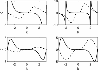
Figure 14: Illustration of $\zeta(k)$ given by (3.46) plotted against wavenumber $k$ for the cases top left: $\rho=1/3$, $\mu=3$, ($m=1$, $M=3$); top right: $\rho=1/3$, $\mu=0.3$, ($m=10$, $M=3$); bottom left: $\rho=3$, $\mu=3$, ($m=1$, $M=3$); bottom right: $\rho=3$, $\mu=0.3$, ($m=10$, $M=3$). The thick solid lines correspond to the acoustic mode and the thick dashed lines to the optical mode. In all cases we take $a=\alpha=1$. In the top two panels, the acoustic cases are scaled down by a factor of 200, in the lower right panel the acoustic case is scaled up by a factor of 10.

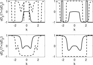
Figure 15: Illustration of wavenumbers where the NLS is of focusing type, that is, $\eta(k)D_{3}(k)>0$ given by (3.45). Due to the varying magnitude of this quantity $\eta D_{3}$, we plot $D_{3}(k)\eta(k)/(1+|D_{3}(k)\eta(k)|)$ against wavenumber $k$ for the cases: top left: $\rho=1/3$, $\mu=3$, ($m=1$, $M=3$); top right: $\rho=1/3$, $\mu=0.3$, ($m=10$, $M=3$); bottom left: $\rho=3$, $\mu=3$, ($m=1$, $M=3$); bottom right: $\rho=3$, $\mu=0.3$, ($m=10$, $M=3$). The solid lines correspond to the acoustic mode and the dashed lines to the optical. In all cases we take $a=\alpha=1$, $b=\beta=2$.

In the case $\zeta=0$, the equation (3.44) has the form of a nonlinear Schrodinger equation, and is of focusing form when $\eta D_{3}>0$ and defocusing form when $\eta D_{3}<0$. The range of wavenumbers where this condition is met is shown in Figure 15. Note that $\eta$ is dependent on $a,b,\alpha,\beta$, in contrast to many of the other parameters that have been introduced; $\eta$ also depends on wavenumber $k$ and linear interaction term $\rho\,$. In particular, by increasing or decreasing $b,\beta$, one can change the sign of $\eta$ so that the condition $\eta D_{3}>0$ is satisfied. In the focusing case, the general breather solution is

$$F_{1}= \;A\exp\left(iKZ+(2D_{3}K^{2}-A^{2}\eta)\frac{iT}{2\Omega}\right)$$

$$\times{\rm sech}\left(\frac{A}{\Omega}\sqrt{\frac{\eta}{2D_{3}}}\left(\Omega Z+2KD_{3}T\right)\right).$$ (3.47)

By absorbing the translation and spatial dependency ($K$) in the exponent into $c$ (3.24), we can assume the simpler form (by putting $K=0$)

$$F_{1}=A{\rm e}^{-i\eta A^{2}T/2\Omega}{\rm sech}\left(AZ\sqrt{\frac{\eta}{2D_{3}}}\right).$$ (3.48)

In cases where $\eta D_{3}<0$, dark breather solutions exist, the general form of these modes are given by

$$F_{1}=R(s){\rm e}^{iWT+i\Phi(s)},\qquad s=z-uT,$$ (3.49)

where, following Remoissenet rembook , $R,\Phi$ are determined by equating real and imaginary parts, namely

$$-\Omega WR+\Omega Ru\Phi^{\prime}= \;\eta R^{3}+D_{3}R^{\prime\prime}-D_{3}R\Phi^{\prime 2},$$ (3.50)

$$-\Omega uR^{\prime}= \;2D_{3}R^{\prime}\Phi^{\prime}+D_{3}R\Phi^{\prime\prime}.$$

Integrating the latter leads to

$$\Phi^{\prime}= \;\frac{K}{D_{3}R^{2}}-\frac{u\Omega}{2D_{3}},$$ (3.51)

and substituting this into the former, (3.50), yields

$$D_{3}R^{\prime\prime}=-\Omega WR-\eta R^{3}+\frac{K^{2}}{D_{3}R^{3}}-\frac{\Omega^{2}u^{2}R}{4D_{3}}.$$ (3.52)

Denoting constants of integration by $K,L$, we integrate this to

$$(2D_{3}RR^{\prime})^{2}= \;LR^{2}-4K^{2}-(4D_{3}W\Omega+u^{2}\Omega^{2})R^{4}$$

$$-2D_{3}\eta R^{6}.$$ (3.53)

The formula

$$R(s)=R_{0}\sqrt{1-\nu{\rm sech}^{2}\left(R_{0}s\sqrt{\frac{-\eta\nu}{2D_{3}}}\right)},$$ (3.54)

provides a solution under the conditions

$$L= \;-2\eta D_{3}R_{0}^{4}(3-2\nu),$$

$$K^{2}= \;-\mbox{$\frac{1}{2}$}\eta D_{3}R_{0}^{6}(1-\nu),$$

$$W= \;-\displaystyle\frac{\eta R_{0}^{2}(3-\nu)}{2\Omega}-\displaystyle\frac{u^{2}\Omega}{4D_{3}}.$$ (3.55)

While the first two merely assign values to the constants of integration, the last provides a necessary relationship for the wavenumber $W$ in terms of the amplitude $R_{0}$, speed $u$ and other parameters. Integrating (3.51), we find

$$\Phi(s)= \;-\frac{u\Omega s}{2D_{3}}+R_{0}s\sqrt{\frac{-\eta(1-\nu)}{2D_{3}}}$$

$$\;+\tan^{\!-1}\left(\sqrt{\frac{\nu}{1\!-\!\nu}}\tanh\left(R_{0}s\sqrt{\frac{-\nu\eta}{2D_{3}}}\right)\right),$$ (3.56)

which, with (3.54), completes the solution for $F_{1}$ (3.49). In the special case $\nu=1$ (where $K=0$), these equations reduce to $K=0$, $\Phi=-u\Omega s/(2D_{3})$, $R=R_{0}\tanh(R_{0}s\sqrt{-\eta/(2D_{3})})$ and hence

$$F_{1}=\; R_{0}\tanh\left(R_{0}(z-uT)\sqrt{\frac{-\eta}{2D_{3}}}\right)$$ (3.57)

$$\times\exp\left(-\frac{iu\Omega}{2D_{3}}(z-uT)-iT\left(\frac{u^{2}\Omega}{4D_{3}}+\frac{\eta R_{0}^{2}}{\Omega}\right)\right),$$

for arbitrary $R_{0},u$. This type of wave has a finite amplitude oscillation over all space, with a decrease in amplitude near $z=uT$.

IV Results

We consider four cases, in increasing complexity: firstly, Case I, where all nonlinearities are symmetric (that is, $a=0=\alpha$ so that $V$ and $W$, given by (2.2) and (2.3) are both even). Secondly, we consider Case II, $\alpha\neq 0=a$; thirdly, $a\neq 0=\alpha$ (Case III), and finally we consider the fully general Case IV where $\alpha\neq 0\neq a$. In all cases, $\beta$ and $b$ are permitted to be nonzero, it is just the cases $\alpha=0$, $a=0$ which allow simpler results to be quoted. The results below hold in the cases of $\beta=0$ and/or $b=0$, the only scenario which is not covered by this analysis is the case where $\alpha=\beta=a=b=0$.

The case $\zeta=0$ occurs when either of the quadratic nonlinearities vanish, that is, $a=0$ or $\alpha=0$ or, when $\alpha a\neq 0$, at isolated values of $k$, such as $k=0,\pi$, as shown in Figure 14. In the case of both quadratic nonlinearities being present, (Case IV, $a\neq 0$ and $\alpha\neq 0$), there may be isolated values of $k$ where $\zeta(k)=0$; however, we might expect any corresponding breather solution to be unstable due to perturbations in the wave number causing the underlying dynamics to become of Ginzburg-Landau form rather than NLS. In the remainder of this section we consider various cases of $a,\alpha=0$ and $a,\alpha\neq 0$ in more detail.

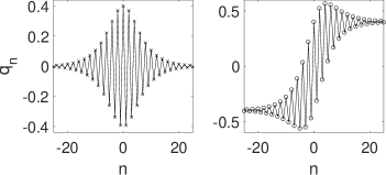
Figure 16: Illustration of the breather wave form (4.1) and breather-kink waveform (4.2). Left: $q_{n}=2h{\rm sech}(hn)\cos(\pi n)$; right: $q_{n}=2h{\rm sech}(hn)\cos(\pi n)+2h\tanh(hn)$ with $h=0.2$ in both cases.

IV.1 Case I: even potentials ($a=0=\alpha$)

Putting $\alpha=0=a$ simplifies the problem considerably. The dispersion relation (3.5) remains, together with $P_{1}=CF_{1}$ with $C=C(k)$ given by (3.12).

In this case we have $S_{0}=G_{0}=0$ from (3.16) and (3.38), $G_{2}=S_{2}=0$ from (LABEL:e2e2eq), but we still have $G_{1},S_{1}$ not necessarily zero (3.29). The envelope speed remains (3.24), and first-correction terms are given by (3.29). The main simplification is that we have $\zeta(k)=0$ in (3.44)–(3.46).

In this case, the breather mode is simple, having no zero-mode contributions from $F_{0}$ or $G_{0},S_{0}$. The leading order solution for the breather is

$$q_{n}(t)\sim 2\epsilon A\cos\left(kn-\omega(k)t-\frac{\epsilon^{2}A^{2}\eta(k)t}{2\Omega(k)}\right)$$

$$\times{\rm sech}\left(\epsilon A(n-ct)\sqrt{\frac{\eta(k)}{2D_{3}(k)}}\right).$$ (4.1)

This form is illustrated in Figure 16. At leading order, we have $Q_{n}(t)=C(k)q_{n}(t)$ with $C(k)$ given by (3.12). Note that this solution is depends on the two parameters, $k$ which governs the wavenumber of the linear carrier wave, and the amplitude $\epsilon A$.

IV.2 Case II: $a=0$, $\alpha\neq 0$

Allowing the force between the inner and outer particles to have a quadratic component ($\alpha\neq 0$, but with $\beta=0$) whilst that of along chain has no quadratic component ($a=0$ with $b\neq 0$) still results in (3.44) being a NLS. The leading order breather solution is again given by (4.1). In this case a zero-mode is produced, that is, $G_{0},S_{0}\neq 0$ by (3.38), however, this is small correction term; and there is no leading order zero mode, since we have $F_{0}=0$ from (3.32). The zero mode (3.38) is localised to the site of the breather.

IV.3 Case III: $a\neq 0$, $\alpha=0$

We now reverse the situation from Sec IV.2. We allow the along chain interactions to have a quadratic component to the force ($a\neq 0$), whilst requiring the force between the inner and outer particles to have only a cubic nonlinearity ($\alpha=0$, $\beta\neq 0$). This again results in (3.44) being a NLS, since $\zeta=0$ for all wavenumbers $k$.

The dispersion relation is given by (3.5), $P_{1}=CF_{1}$ with (3.12). Since $\alpha=0$, from (3.16), we have $G_{0}=S_{0}=0$, however, a zero mode (3.32) is produced due to $F_{0}\neq 0$, this mode is the same for both inner and outer masses. The mode is not localised: given that $F_{1}$ has a sech-shape, $F_{0}$ has a tanh form, so this corresponds to a localised pre-compression of the lattice. In (3.18), there is some simplification, although second harmonic terms are still generated. From (3.38), we find $G_{0}=S_{0}=0$, so the only zero-mode we are concerns is due to $F_{0}$.

The leading order solution (4.1) is replaced by the more general kink-breather combination

$$q_{n}(t)\sim 2\epsilon A\cos\left(kn-\omega(k)t-\frac{\epsilon^{2}A^{2}\eta t}{2\Omega}\right)$$

$$\!\times{\rm sech}\left(\epsilon A(n-ct)\sqrt{\frac{\eta}{2D_{3}}}\right)$$ (4.2)

$$\!\!+\!\frac{8\epsilon aA\sin^{2}(\mbox{$\frac{1}{2}$}k)\sqrt{2D_{3}}}{\sqrt{\eta}[(M\!+\!m)c^{2}-1]}\!\tanh\!\left(\frac{\epsilon A(n-ct)\sqrt{\eta}}{\sqrt{2D_{3}}}\right).$$

This form is illustrated in Figure 16.

IV.4 Case IV: the general case $a\neq 0\neq\alpha$

For $a\neq 0\neq\alpha$, equation (3.44) is of complex Ginzburg-Landau form (CGL), rather than an NLS equation. For some values of the wavenumber $k$, we may have $\zeta(k)=0$ and so the NLS derivation is valid; however, for general values of $k$, we expect $\zeta(k)\neq 0$, and so different dynamics may be observed. When $\zeta=0$, it is natural to consider this as a combination of Cases II and III, (Secs IV.2 & IV.3), so that both the leading order nonlocal zero mode, $F_{0}$ (which is the same for both inner and outer masses), and the smaller, localised zero modes $G_{0}\neq S_{0}$ are present, the latter giving different amplitudes for the inner and outer masses. For example, if we consider the special case $k=\pi$, then we find $c=0=\gamma_{1}=G_{1}=S_{1}=G_{0}=\widehat{a}_{g}=\widehat{a}_{s}$, and $\zeta=0$, so the NLS reduction remains valid, and long-lived stationary breather-modes may be expected to exist.

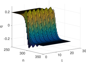
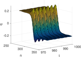
Figure 17: Results of numerical simulations of the full ODE system. The system is simulated using Matlab ode45 matlab with $N=400$ lattice sites, and parameter values given by $\rho=3$, $m=3$, $M=1$, $\epsilon=0.1$, $\mu=1/3$, $\rho\,=3$, $a=0.5$, $b=0.5$, $\beta=2$, $\alpha=0.5$, $k=\pi$. The plots show the resulting acoustic mode at the start and end of a simulation of length $t_{max}=1000$. In colour in online version.

In Figure 17 we illustrate the results of a numerical simulation of the system (2.4)–(2.5), started with initial conditions given by $k=\pi$ in the leading order terms ($F_{0},F_{1},P_{0},P_{1}$) from (3.2)–(3.3), namely (3.48) and (3.32). This corresponds to Case IV, since $\alpha\neq 0\neq\beta$ and $a\neq 0\neq b$. We have neglected the second order and all higher terms ($G_{j},H_{j},S_{j},R_{j},\ldots$); the initial conditions are an approximation to the mode. Over early times ($0<t<\sim 10^{2}$), there is a very small adjustment in the shape of the mode over longer times, the mode appears stable. The system has a small amount of damping built into lattice sites $1\neq n\leq 40$ and $360\leq n\leq 400$ in order to dampen the radiation which is shed from the mode at early times. This takes the form of additional terms $-\lambda\mbox{d}q_{n}/\mbox{d}t$ and $-\lambda\mbox{d}Q_{n}/\mbox{d}t$ added to equations (2.4)–(2.5) with $\lambda=0.03$.

When $\zeta\neq 0$, (3.44) has the form of a complex Ginzburg Landau equation (CGL), which exhibits markedly different behaviour from NLS. The CGL equation is typically written as

$$F_{1,T}=\delta F_{1}+(1+i\chi)F_{1,XX}+(1+i\zeta)|F_{1}|^{2}F_{1}.$$ (4.3)

Our case (3.44) corresponds to the limit $\chi\gg 1$, with $X\gg 1$, $\zeta=\mathcal{O}(1)$, and $\delta=0$. In these cases the equation (3.44) does not have stable pulse-type solutions. Instead, solutions of (3.44) either decay to zero or blow up according to the sign of $\xi$. We find that norm of the distribution $F_{1}$ evolves according to

$$\Omega\frac{\mbox{d}}{\mbox{d}t}\int|F_{1}|^{2}\,\mbox{d}z= \;2\zeta\int|F_{1}|^{4}\,\mbox{d}z,$$ (4.4)

thus if $\zeta>0$, then $\int|F_{1}|^{2}\mbox{d}z$ monotonically increases and if $\zeta<0$ then $\int|F_{1}|^{2}\mbox{d}z$ monotonically decreases. Similarly, the NLS Hamiltonian is not conserved when $\zeta\neq 0$. If we define

$$H=\int D_{3}|F_{1,z}|^{2}-\mbox{$\frac{1}{2}$}\eta|F_{1}|^{4}\,\mbox{d}z,$$ (4.5)

then we find

$$\!\frac{\mbox{d}H}{\mbox{d}t}= \;\frac{\zeta D_{3}}{\Omega}\!\int 4|F_{1}F_{1,z}|^{2}+F_{1}^{2}F_{1,z}^{*2}+F_{1}^{*2}F_{1,z}^{2}-\frac{2\eta}{D_{3}}|F_{1}|^{6}\,\mbox{d}z.$$

A full discussion of the dynamics exhibted by the Ginzburg-Landau equation is beyond the scope of this paper, we refer the interested reader to the wider literature, for example, the introductions provided by Garcia-Morales & Krischer GL-intro2 and Hohenberg & Krekhov GL-intro1 .

V Conclusions

We have considered the fully nonlinear problem of a mass-in-mass FPUT chain in which both the along-chain interactions and the interaction between the inner and outer masses are nonlinear. We have used multiple scales asymptotics to construct an explicit form for the breather in the small amplitude limit. This involves solving systems of equations at each order of magnitude and for each harmonic frequency, using a Fredholm consistency condition to generate additional solution criteria. In many cases, this ultimately yields a nonlinear Schrodinger equation.

Many asymptotic approximations of breathers require the calculation of the “zero”-mode corrections at $\mathcal{O}(\epsilon^{2}{\rm e}^{0i\theta})$, from equations at $\mathcal{O}(\epsilon^{4}{\rm e}^{0i\theta})$. Often this requires knowledge of the leading order term, so giving a coupled problem. However, in the case analysed here, the equations at $\mathcal{O}(\epsilon^{2}{\rm e}^{0i\theta})$ and $\mathcal{O}(\epsilon^{4}{\rm e}^{0i\theta})$ give explicit formulae for $G_{0},S_{0}$. This enables us to calculate a single NLS equation for the leading order shape, $F_{1}$.

In addition to illustrating properties of the solution for various choices of the masses, we have given simplified asymptotic forms for the solution in the cases where the ratio of the inner to outer masses is extremely small or extremely large. In future work reem , we propose to use numerical techniques to investigate the stability, robustness, and other properties of breather solutions in this system, in both the cases $a=0$ and $a\neq 0$.

Acknowledgements

I am grateful to Paul Matthews for helpful conversations regarding the complex Ginzburg-Landau system. I am grateful to Reem Almarashi for writing some of the code which produced Figure 17. My thanks also go to the referees for making helpful comments to improve the manuscript.

Appendix A Asymptotics of travelling wave solutions

Below, we derive the small amplitude travelling wave solutions for the fully nonlinear lattice. The results show that the nonlinear nearest-neighbour interactions control the shape of the waves, and that the nonlinear interaction between inner and outer masses is only relevant in higher order terms. There are two separate cases to consider as different asymptotic scalings are required for the cubic ($a\neq 0$) and quartic ($a=0$) nearest neighbour potential energy functions.

A1 Quartic potential, $a=0$, $b\neq 0$

Here we leave $\alpha,\beta$ arbitrary. The governing ODEs are

$$\!\!m\frac{\mbox{d}^{2}q_{n}}{\mbox{d}t^{2}}\!= q_{n+1}\!-\!2q_{n}\!+\!q_{n-1}\!+\!b(q_{n+1}\!-\!q_{n})^{3}\!-\!b(q_{n}\!-\!q_{n-1})^{3}$$

$$-\rho(q_{n}-Q_{n})-\alpha(q_{n}-Q_{n})^{2}-\beta(q_{n}-Q_{n})^{3},$$

$$\!\!\!\!M\frac{\mbox{d}^{2}Q_{n}}{\mbox{d}t^{2}}= \;\rho(q_{n}-Q_{n})+\alpha(q_{n}-Q_{n})^{2}+\beta(q_{n}-Q_{n})^{3}.$$

We replace $(q_{n}(t),Q_{n}(t))$ by $(q(y,\tau),Q(y,\tau))$ using the scaled variables

$$y=hn,\qquad\tau=ht,\qquad h\ll 1,$$ (A3)

$$Q=q-h^{2}W,\qquad M=\mu m,$$ (A4)

to obtain the approximating PDEs

$$mq_{\tau\tau}= \;q_{yy}+\mbox{$\frac{1}{12}$}h^{2}q_{yyyy}+bh^{2}(q_{y}^{3})_{y}-\rho W-\alpha h^{2}W^{2},$$ (A5)

$$\mu mq_{\tau\tau}= \;\rho W+\alpha h^{2}W^{2}+h^{2}\mu mW_{\tau\tau},$$ (A6)

where we have neglected terms of $\mathcal{O}(h^{4})$ and higher.

If we assume a TW of the form $q(y,\tau)=q(z)$, $Q(y,\tau)=Q(z)$, $W(y,\tau)=W(z)$, where $z=y-c\tau$, then we obtain the system of ODEs

$$(mc^{2}-1)q^{\prime\prime}+\rho W= \;h^{2}\left[\mbox{$\frac{1}{12}$}h^{2}q^{\prime\prime\prime\prime}+3b(q^{\prime 2})q^{\prime\prime}-\alpha W^{2}\right],$$ (A7)

$$\mu mc^{2}q^{\prime\prime}-\rho W= \;h^{2}\left[\alpha W^{2}+\mu mc^{2}W^{\prime\prime}\right].$$ (A8)

At leading order, we thus have

$$W=\frac{\mu mc^{2}q^{\prime\prime}}{\rho}=\frac{(1-mc^{2})q^{\prime\prime}}{\rho},$$ (A9)

which provides an equation for the expected speed of the wave, $c=c_{0}$. We consider waves which travel at speeds close to $c_{0}$, and hence, we write

$$c=c_{0}(1+c_{1}h^{2}), \quad c_{0}=\frac{1}{\sqrt{m(1+\mu)}}.$$ (A10)

Adding (A7) and (A8) together with $c$ being given by (A10) and $W$ by (A9) implies

$$2c_{1}q^{\prime\prime} =\;\gamma q^{\prime\prime\prime\prime}+3bq^{\prime 2}q^{\prime\prime},$$ (A11)

$$\gamma =\;\mbox{$\frac{1}{12}$}+\frac{\mu^{2}}{\rho(1\!+\!\mu)^{2}}.$$ (A12)

After integrating with constants of integration set to zero, so that $q^{\prime},q^{\prime\prime}\rightarrow 0$ as $z\rightarrow\pm\infty$, we obtain the solution

$$q=\pm\sqrt{\frac{2\gamma}{b}}\tan^{-1}\left(\sinh\left((y-c\tau)\sqrt{\frac{2c_{1}}{\gamma}}\right)\right).$$ (A13)

We note that both this leading order solution, and that for $Q\sim q+\mathcal{O}(h^{2})$, are independent of $\alpha,\beta$, depending only on $\rho,\mu,b,c_{1}$, with $c$ being given by (A10).

A2 Cubic potential, $a\neq 0$, $b=0$

We again leave $\alpha,\beta$ arbitrary, giving the governing ODEs

$$\!\!m\frac{\mbox{d}^{2}q_{n}}{\mbox{d}t^{2}}\!= q_{n+1}\!-\!2q_{n}\!+\!q_{n-1}\!+\!a(q_{n+1}\!-\!q_{n})^{2}\!-\!a(q_{n}\!-\!q_{n-1})^{2}$$

$$-\rho(q_{n}-Q_{n})-\alpha(q_{n}-Q_{n})^{2}-\beta(q_{n}-Q_{n})^{3},$$

$$\!\!\!M\frac{\mbox{d}^{2}Q_{n}}{\mbox{d}t^{2}}= \;\rho(q_{n}-Q_{n})+\alpha(q_{n}-Q_{n})^{2}+\beta(q_{n}-Q_{n})^{2}.$$

We follow the same procedure as in §A1, namely applying (A3)–(A4), which leads to the hence the approximating PDEs

$$mq_{\tau\tau}= \;q_{yy}+\mbox{$\frac{1}{12}$}h^{2}q_{yyyy}+ah(q_{y}^{2})_{y}-\rho W-\alpha h^{2}W^{2},$$ (A16)

$$\mu mq_{\tau\tau}= \;\rho W+\alpha h^{2}W^{2}+h^{2}\mu mW_{\tau\tau}.$$ (A17)

Here, as well as the leading-order terms, we have retained terms of $\mathcal{O}(h)$ and $\mathcal{O}(h^{2})$ but neglected terms higher than these. We now assume a TW, writing

$$q(y,\tau)=hu(z),\quad W(y,\tau)=hw(z),\quad z=y-c\tau,$$

to obtain

$$(mc^{2}-1)u^{\prime\prime}+\rho w= \;h^{2}\left[\mbox{$\frac{1}{12}$}u^{\prime\prime\prime\prime}+a(u^{\prime 2})^{\prime}\right],$$ (A19)

$$\mu mc^{2}u^{\prime\prime}-\rho w= \;h^{2}\mu mc^{2}w^{\prime\prime}.$$ (A20)

At leading order, we thus have

$$w=\frac{\mu mc^{2}u^{\prime\prime}}{\rho}=\frac{(1-mc^{2})u^{\prime\prime}}{\rho},$$ (A21)

which gives the same expression for $c_{0}$ as previously (A10). Combining (A19)–(A21) with (A10)

$$2c_{1}u^{\prime\prime} =\;\gamma u^{\prime\prime\prime\prime}+2au^{\prime}u^{\prime\prime},$$ (A22)

with $\gamma$ as defined by (A12). After integrating with all constants of integration set to zero, so that $u^{\prime},u^{\prime\prime}\rightarrow 0$ as $z\rightarrow\pm\infty$, we find the solution

$$u =\;\frac{3}{a}\sqrt{2\gamma c_{1}}\,\tanh\left((y-c\tau)\sqrt{\frac{c_{1}}{\gamma}}\right).$$ (A23)

As with the quartic potential case, at leading order, the solution has no dependence on $\alpha,\beta$, it only depends on $\mu,\rho,c_{1},a$.

Appendix B Special solutions of the Ginzburg-Landau equation (3.44)

Due to the fully quadratic case ($\alpha\neq 0\neq a$, considered in Sec.  IV.4) being governed by the Ginzburg-Landau equation rather than than the NLS (Sec IV.1), we expect that the form and stability of waves in the case $\alpha\neq 0\neq a$ could differ from those cases with the more standard reduction to NLS, where, for some lattice systems, large-time stability results have been derived, see for example, pego ; dp ; ober ; HamLatDynMinE .

The form of some special solutions of the Ginzburg-Landau equation (3.44) can be obtained from the ansatz

$$F_{1}(z,T)=A(Z)\exp\left(i\Phi(Z)+i\widetilde{\omega}T\right),\quad Z=z-uT,$$ (B24)

which leads to the coupled ODEs for the real functions $A(Z),\phi(Z)$

$$\Omega uA\Phi^{\prime}-\widetilde{\omega}\Omega A= \;\eta A^{3}+D_{3}A^{\prime\prime}-D_{3}A(\Phi^{\prime})^{2},$$ (B25)

$$-\Omega uA^{\prime}= \;\zeta A^{3}+D_{3}A\Phi^{\prime\prime}+2D_{3}A^{\prime}\Phi^{\prime}.$$ (B26)

We seek solutions in which $A(Z)$ is single-humped and decays to zero in both limits $Z\rightarrow\pm\infty$.

We introduce $S(Z)$ defined by $S^{\prime}(Z)=A(Z)^{4}$ whereupon the latter equation (B26) implies

$$\frac{\mbox{d}}{\mbox{d}Z}\left(D_{3}A^{2}\Phi^{\prime}+\mbox{$\frac{1}{2}$}u\Omega A^{2}\right)=-\zeta A^{4}=-\zeta\frac{\mbox{d}S}{\mbox{d}Z},$$ (B27)

and the former equation (B25) gives

$$\left(\!D_{3}A^{2}\Phi^{\prime}\!+\!\frac{u\Omega A^{2}}{2}\!\right)^{\!\!2}\!= \;D_{3}A^{4}\left[\frac{D_{3}A^{\prime\prime}}{A}\!+\!\eta A^{2}\!+\!\Omega\widetilde{\omega}\!+\!\frac{u^{2}\Omega^{2}}{4D_{3}}\right].$$

(B28)

Integrating (B27) and substituting in (B28), we find

$$\zeta^{2}S^{2}= \;\frac{D_{3}S^{\prime}}{4}\left[\frac{D_{3}S^{\prime\prime\prime}}{S^{\prime}}-\frac{3D_{3}S^{\prime\prime 2}}{4S^{\prime 2}}+4\eta\sqrt{S^{\prime}}\right.$$

$$\left.\qquad\qquad+4\Omega\widetilde{\omega}+\frac{u^{2}\Omega^{2}}{D_{3}}\right].$$ (B29)

Since we seek solutions in which $A(Z)$ has the form of a pulse, $S(Z)$ will have the form of a kink-wave, which can be assumed to be monotonically increasing. As (B29) is autonomous, we rewrite it as a non-autonomous second-order equation using

$$P(S)= \;\frac{\mbox{d}S(Z)}{\mbox{d}Z},\quad Z=\int\frac{\mbox{d}S}{P(S)},$$ (B30)

so that

$$S^{\prime\prime}(Z)=P(S)P^{\prime}(S), \quad S^{\prime\prime\prime}=P(PP^{\prime})^{\prime}=P^{2}P^{\prime\prime}+PP^{\prime 2}.$$

We expect $P(S)>0$ with $P(0)=0$ and $P(S_{1})=0$ for some $S_{1}>0$. Hence

$$\frac{4\zeta^{2}S^{2}}{D_{3}P}= D_{3}(PP^{\prime\prime}\!+\!\mbox{$\frac{1}{4}$}P^{\prime 2})+4\eta\sqrt{P}+4\Omega\widetilde{\omega}+\frac{u^{2}\Omega^{2}}{D_{3}}.$$

(B32)

which can be simplified by the substitution $P=R^{4/5}$

$$\mbox{$\frac{1}{5}$}D_{3}R^{\prime\prime}+\eta R^{-1/5}+\left(\widetilde{\omega}+\frac{u^{2}\Omega}{4D_{3}}\right)R^{-3/5}= \;\frac{\zeta^{2}S^{2}}{D_{3}R^{7/5}}.$$

(B33)

By considering the asymptotic behaviour of this in the limit $Z\rightarrow 0$ where $A\rightarrow 0$, we note qualitative differences between the classic NLS limit when $\zeta=0$, and the GL limit when $\zeta\neq 0$. This limit corresponds to $S\rightarrow S_{0}>0$ and $P,R\rightarrow 0$.

When $\zeta=0$ the leading order balance is given by one of

$$\mbox{$\frac{1}{5}$}D_{3}R^{\prime\prime}\sim \;BR^{-3/5},\quad B:=\widetilde{\omega}\Omega+\frac{u^{2}\Omega^{2}}{4D_{3}},$$

$$\mbox{$\frac{1}{5}$}D_{3}R^{\prime\prime}\sim \;-\eta R^{-1/5},$$ (B34)

the second case occurring if $B=0$. Writing $R(S)\sim R_{0}(S_{0}-S)^{\gamma}$, these correspond to the equations

$$\gamma=\mbox{$\frac{5}{4}$},\quad Z\sim\log|S_{0}-S|,$$ (B35)

$$\gamma=\mbox{$\frac{5}{3}$},\quad Z\sim(S_{0}-S)^{-1/3}.$$ (B36)

Here we have made use of $R=P^{5/4}$ and (B30), and find $Z\rightarrow\infty$ as $S\rightarrow S_{0}$, and hence $A\rightarrow 0$. The first case has exponential convergence ($A\sim{\rm e}^{-\lambda Z}$), whilst the latter, algebraic decay ($A\sim z^{-4}$).

However, in the case $\zeta\neq 0$, the leading order balance in (B33) is

$$\mbox{$\frac{1}{5}$}D_{3}R^{\prime\prime}\sim\frac{\zeta^{2}S_{0}^{2}}{D_{3}R^{7/5}},$$ (B37)

hence we have $\gamma=5/6$ and $P^{5/4}=R\sim(S_{0}-S)^{5/6}$,

$$P=\frac{\mbox{d}S}{\mbox{d}Z}\sim(S_{0}-S)^{2/3},$$ (B38)

which implies $-Z\sim(S_{0}-S)^{1/3}$, and $Z\rightarrow 0$ as $S\rightarrow S_{0}$, rather than $Z\rightarrow\infty$ as $S\rightarrow S_{0}$. Thus, whilst the GL reduction may give rise to periodic waves, and waves of a more complicated form than those derived from the NLS, we do not expect to see single-humped pulse solitons, with exponentially-decaying tails.

References

- [1] R. Almarashi, R. Nicks, J.A.D. Wattis. In preparation, (2022).
- [2] J.F.R. Archilla, N. Jiminez, V.J. Sanchez-Morcillo, L.M. Garcia-Raffi. Quodons in Mica. Nonlinear Localized Travelling Excitations in Crystals. Springer Series in Materials Science, vol 221. (2015).
- [3] J. Bajars, J.C. Eilbeck, B. Leimkuhler. Nonlinear propagating localized modes in a 2D hexagonal crystal lattice. Physica D, 301–302, 8–20, (2015).
- [4] C.M. Bender, S. Orszag. Advanced Mathematical Methods for Scientists and Engineers. Springer, New York (1978).
- [5] L. Bonanomi, G. Theocharis, and C. Daraio, Wave propagation in granular chains with local resonances. Phys. Rev. E, 91, 033208, (2015).
- [6] I.A. Butt, J.A.D. Wattis. Discrete breathers in a two-dimensional Fermi-Pasta-Ulam lattice. J. Phys. A; Math. Gen., 39, 4955–4984, (2006).
- [7] I.A. Butt, J.A.D. Wattis. Discrete breathers in a two-dimensional hexagonal Fermi-Pasta-Ulam lattice. J. Phys. A; Math. Theor., 40, 1239–1264, (2007).
- [8] C. Chong, P.G. Kevrekedis, G. Theocharis, C. Daraio, Dark Breathers in granular crystals. Phys. Rev. E, 87, 042202, (2013).
- [9] T. Cretegny, R. Livi, M. Spicci, Breather dynamics in diatomic FPU chains. Physica D, 119, 88-98, (1998).
- [10] E. Fermi, J. Pasta, S. Ulam, Studies of nonlinear problems. Los Almos Scientific Laboratory report LA-1940, (1955). Reprinted in: Lect. in Appl. Math., 15, 143–156, (1974)
- [11] S. Flach, K. Kladko, R.S. MacKay. Energy thresholds for discrete breathers in one- two- and three-dimensional lattices. Phys. Rev. Lett., 78, 1207–1210, (1997).
- [12] G. Friesecke, J.A.D. Wattis. Existence theorem for travelling waves on lattices, Commun. Math. Phys., 161, 391–418, (1994).
- [13] G. Friesecke, R.L. Pego. Solitary waves on FPU lattices: I. Qualitative properties, renormalization and continuum limit. Nonlinearity, 12, 1601–1628, (1999).
- [14] V. Garcia-Morales, K. Krischer. The complex Ginzburg-Landau equation: an introduction. Contemporary Physics, 53, 79-95, (2012).
- [15] P.C. Hohenberg, A.P. Krekhov, An introduction to the Ginzburg-Landau theory of phase transitions and non-equilibrium patterns. Physics Reports, 572, 1-42, (2015).
- [16] G. James, D. Pelinovsky, Z. Rapti, G. Schneider. Lattice Differential Equations. Oberwolfach Reports, 130, 2631–268, (2013).
- [17] A. Khan, D.E. Pelinovsky, Long-time stability of small FPU solitary waves. Disc. & Cont. Dyn. Syst., 34, 2065–2075, (2017).
- [18] P.G. Kevrekidis, A Vainchtein, M. Serra Garcia, C. Daraio. Interaction of travelling waves with mass-with-mass defects within a Hertzian chain. Phys. Rev. E, 87, 042811, (2013).
- [19] P.G. Kevrekidis, A.G. Stefanov, H. Xu, Traveling waves for the mass in mass model of granular chains. Lett. Math. Phys., 106, 1067–1088, (2016).
- [20] A. Leonard, C. Chong, P.G. Kevrekidis, C. Daraio. Traveling waves in 2D hexagonal granular crystal lattices. Granular Matter, 16, 531, (2014).
- [21] L. Liu, G. James, P.G. Kevrekidis, A. Vainchtein, Strongly nonlinear waves in locally resonant granular chains Nonlinearity, 29, 3496–3527, (2016).
- [22] L. Liu, G. James, P. Kevrekidis, A. Vainchtein, Breathers in a locally resonant granular chain with precompression. Physica D,331, 27–47, (2016).
- [23] R. Livi, M. Spicci, R.S. MacKay, Breathers on a diatomic FPU chain. Nonlinearity 10, 1421–1434, (1997).
- [24] J. Lydon, M. Serra-Garcia, and C. Daraio, Local to extended transitions of resonant defect mode. Phys. Rev. Lett., 113, 185503, (2014).
- [25] R.S. Mackay S. Aubry, Proof of existence of breathers from time-reversible or Hamiltonian networks of weakly-coupled oscillators. Nonlinearity, 7, 1623–1643, (1994)
- [26] J.L. Marin, J.C. Eilbeck, F.M. Russell. Breathers in cuprate-like lattices, Phys. Lett. A, 281, 21–25, (2001).
- [27] J.L. Marin, J.C. Eilbeck, F.M. Russell. Localised moving breathers in a 2D hexagonal lattice, Phys. Lett. A, 248, 225–229, (1998).
- [28] Matlab, The MathWorks, Inc. (2020).
- [29] S. Paleari, T. Penati, Hamiltonian Lattice Dynamics. Mathematics in Engineering, 1, 881–887, (2019).
- [30] M Remoissenet. Waves Called Solitons, Springer-Verlag, Berlin, (1999).
- [31] S.P. Wallen, J. Lee, D. Mei, C. Chong, P.G. Kevrekidis, N. Boechler. Discrete breathers in a mass-in-mass chain with Hertzian local resonators. Phys. Rev. E, 95, 022904, (2017).
- [32] J.A.D. Wattis. Travelling waves in the diatomic FPU lattice. AIMS Mathematics in Engineering, 1, 327–342, (2019).
- [33] J.A.D. Wattis, A.S.M. Alzaidi, Asymptotic analysis of breather modes in a two-dimensional mechanical lattice. Physica D, 401, 132207, (2020).
- [34] N.J. Zabusky, M.D. Kruskal, Interaction of “solitons” in a collisionless plasma and the recurrence of initial states. Phys. Rev. Lett., 15, 240–243, (1965).