Many-body localization and delocalization dynamics in the thermodynamic limit

Abstract

Disordered quantum systems undergoing a many-body localization (MBL) transition fail to reach thermal equilibrium under their own dynamics. Distinguishing between asymptotically localized or delocalized dynamics based on numerical results is however nontrivial due to finite-size effects. Numerical linked cluster expansions (NLCE) provide a means to tackle quantum systems directly in the thermodynamic limit, but are challenging for models without translational invariance. Here, we demonstrate that NLCE provide a powerful tool to explore MBL by simulating quench dynamics in disordered spin-$1/2$ two-leg ladders and Fermi-Hubbard chains. Combining NLCE with an efficient real-time evolution of pure states, we obtain converged results for the decay of the imbalance on long time scales and show that, especially for intermediate disorder below the putative MBL transition, NLCE outperform direct simulations of finite systems with open or periodic boundaries. Furthermore, while spin is delocalized even in strongly disordered Hubbard chains with frozen charge, we unveil that an additional tilted potential leads to a drastic slowdown of the spin imbalance and nonergodic behavior on accessible times. Our work sheds light on MBL in systems beyond the well-studied disordered Heisenberg chain and emphasizes the usefulness of NLCE for this purpose.

Introduction.– Many-body localization (MBL) extends Anderson localization to interacting quantum systems Nandkishore2015 ; Abanin2019 . Based on seminal early works Gornyi2005 ; Basko2006 , and numerous subsequent studies (see e.g. Oganesyan2007 ; Pal2010 ; Imbrie2016 ; Berkelbach2010 ; Luitz2015 ; Kjall2014 ; Bera2015 ), it is believed that disordered one-dimensional (1d) system with local interactions can undergo a transition from a thermal phase to a MBL phase for sufficiently strong disorder. The MBL phase is characterized, e.g., by a breakdown of the eigenstate thermalization hypothesis Dallesio2016 , area-law entangled energy eigenstates Bauer2013 , and a logarithmic growth of entanglement in time Znidaric2008 ; Bardarson2012 . Its properties can be understood in terms of an emergent set of local integrals of motion Serbyn2013 ; Huse2014 ; Chandran2015 ; Ros2015 , so-called l-bits. Due to a finite overlap with these l-bits, observables fail to thermalize under time evolution, which makes MBL systems candidates for realizing quantum memories. This memory of initial conditions is a key experimental signature of MBL Schreiber2015 ; Choi2016 ; Smith2016 , but is theoretically investigated as well Luitz2017 ; Enss2017 ; Nico-Katz2021 .

The emergent l-bit phenomenology of MBL motivated by nearest-neighbor qubit models can become unstable in higher dimensions Choi2016 ; Wahl2019 ; Decker2021 ; Chertkov2021 , in the presence of non-Abelian symmetries parameswaran2018many ; potter2016symmetry ; protopopov2017effect ; protopopov2020non , long-range interactions Yao2014 ; Burin2015 ; Nandkishore2017 ; Modak2020 , large local Hilbert-space dimensions Richter2019_2 ; Richter2020_3 ; Schliemann2021 , and disorder-free systems Grover2014 ; Schiulaz2014 ; Brenes2018 ; Heitmann2020 ; Smith2017 ; Yao2016 ; Sirker2019 ; Schulz2019 ; vanNieuwenburg2019 ; Karpov2021 . Despite of these instabilities of the fully many-body localized systems, they can show anomalously slow dynamics and even nonergodic behavior for certain initial conditions Gopalakrishnan2020 , referred to as MBL regime Morningstar2021 . For instance, in two dimensions (2d) signatures of the MBL regime exist in experiments and numerics Choi2016 ; Wahl2019 ; Decker2021 ; Chertkov2021 , although in the thermodynamic limit the avalanche picture DeRoeck2017 ; Doggen2020 suggests fully chaotic dynamics, albeit at astronomically long time scales.

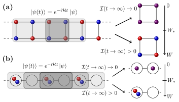
Figure 1: We study the imbalance ${\cal I}(t)$ in disordered (a) two-leg spin ladders and (b) Fermi-Hubbard chains. (Disorder not shown here.) For $W<W_{\ast}$, ${\cal I}(t)$ is expected to decay to zero, while ${\cal I}(t)>0$ in the MBL phase for $W>W_{\ast}$. NLCE is used to simulate ${\cal I}(t)$ in the thermodynamic limit $L\to\infty$. Within NLCE, ${\cal I}(t)$ is obtained on finite clusters (shaded rectangles), whose contributions are suitably combined to yield quantum dynamics without finite-size effects SuppMat .

The main complication for numerical studies of MBL is the presence of strong finite-size effects Weiner2019 ; Panda2020 ; Sierant2021 ; Doggen2018 ; Abanin2021 ; Sierant2020 ; Morningstar2021 . In this context, the existence of a genuine MBL phase (even for nearest-neighbor 1d models) has been put into question Suntajs2020 ; Kiefer-Emmanouilidis2020 ; Sels2021 . Providing a definite answer to this issue by means of numerical approaches is challenging. On one hand, full or sparse-matrix diagonalization methods are restricted to intermediate system sizes, potentially leading to inconclusive results. On the other hand, tensor-network techniques can treat large systems, but the times reachable in simulations are limited by the growth of entanglement Paeckel2019 . Despite notable progress to extend these time scales Doggen2018 ; Doggen2020 , and the development of other sophisticated methods Burau2021 ; Thomson2018 ; Kvorning2021 , studying quantum many-body dynamics, especially beyond 1d, remains difficult Kennes2018 ; Hubig2019 ; Kshetrimayum2020 .

In this Letter, we study the nature of the MBL regime in two classes of disordered models (see Fig. 1), (i) spin-$1/2$ two-leg ladders Doggen2020 ; Baygan2015 ; Wiater2018 ; Hauschild2016 , a quasi one-dimensional system which represents an intermediate case between a 1d chain and a 2d lattice, and (ii) Fermi-Hubbard (FH) chains Prelovsek2016 ; Mondaini2015 ; Kozarzewski2018 ; Zakrzewski2018 ; Iadecola2019 ; Protopopov2019 ; Kurlov2021 , where disorder only couples to the charge degrees of freedom. Both of them can also be viewed as 1d models with local Hilbert-space dimension greater than two. In the FH chain, there is a SU$(2)$ symmetry incompatible with MBL, and we also study the effect of a tilted potential which can induce Stark MBL Schulz2019 ; vanNieuwenburg2019 ; Guo2021 .

We demonstrate that numerical linked cluster expansions (NLCE) Tang2013 provide a powerful means to study the MBL regime. The crucial advantage of NLCE is that, if converged, they yield results directly in the thermodynamic limit, i.e., there are no finite-size effects. We use NLCE to study the dynamics resulting from out-of-equilibrium initial states and obtain converged results for the imbalance ${\cal I}(t)$ on long time scales, outperforming direct simulations of finite systems with open or periodic boundaries especially for intermediate disorder $W<W_{\ast}$, which allows the extraction of more accurate lower bounds for $W_{\ast}$. Furthemore, we show that, in contrast to strongly disordered FH chains where spin thermalizes despite charge being localized, an additional tilted potential leads to a slowdown of the spin imbalance and nonergodic behavior for certain initial states.

Models & Observables.– The first class of models we consider are disordered Heisenberg two-leg spin ladders,

$${\cal H}_{\text{SL}}=\sum_{k=1}^{2}\sum_{\ell}\left({\bf S}_{\ell,k}{\bf S}_{\ell+1,k}+h_{\ell,k}S_{\ell,k}^{z}\right)+\sum_{\ell=1}^{L}{\bf S}_{\ell,1}\cdot{\bf S}_{\ell,2}\ ,$$ (1)

where ${\bf S}_{\ell,k}=(S_{\ell,k}^{x},S_{\ell,k}^{y},S_{\ell,k}^{z})$ are spin-$1/2$ operators on leg $k$ and rung $\ell$, $L$ denotes the length of the ladder ($2L$ lattice sites in total), and the on-site fields $h_{\ell,k}\in[-W,W]$ are randomly drawn from a uniform distribution with $W$ setting the strength of disorder. We study the nonequilibrium dynamics resulting from quenches with antiferromagnetic initial states of the form [cf. Fig. 1 (a)],

$$\ket{\psi(0)}=\left|\begin{array}[]{cccccccc}\cdots&\downarrow&\uparrow&\downarrow&\uparrow&\downarrow&\uparrow&\cdots\\ \cdots&\uparrow&\downarrow&\uparrow&\downarrow&\uparrow&\downarrow&\cdots\\ \end{array}\right\rangle\ ,$$ (2)

in the $\sum_{k,\ell}S_{\ell,k}^{z}=0$ sector. We monitor the imbalance, ${\cal I}(t)=\sum_{k}\sum_{\ell}(-1)^{k+\ell}\langle S_{\ell,k}^{z}(t)\rangle/L$, where $\langle\cdot(t)\rangle=\bra{\psi(t)}\cdot\ket{\psi(t)}$, $\ket{\psi(t)}=e^{-i{\cal H}t}\ket{\psi(0)}$, and ${\cal I}(0)=1$. In case of thermalization, one expects $\lim_{t\to\infty}\lim_{L\to\infty}{\cal I}(t)\to 0$. In contrast, ${\cal I}(t)>0$ in the case of MBL, see Fig. 1. Distinguishing between asymptotically localized or delocalized dynamics is challenging due to (i) finite-size effects and (ii) finite simulation times. In this Letter, we show that NLCE provide a means to mitigate the impact of (i) by obtaining ${\cal I}(t)$ in the thermodynamic limit $L\to\infty$.

As a second model, we study disordered FH chains,

$${\cal H}_{\text{FH}}=-\sum_{\ell,\sigma}(c_{\ell,\sigma}^{\dagger}c_{\ell+1,\sigma}+\text{h.c.})+\sum_{\ell=1}^{L}(Un_{\ell,\uparrow}n_{\ell,\downarrow}+\mu_{\ell}n_{\ell})\ ,$$ (3)

where $c_{\ell,\sigma}^{\dagger}$ ($c_{\ell,\sigma}$) creates (annihilates) a fermion of spin $\sigma$ at site $\ell$, $U$ is the on-site interaction, $n_{\ell,\sigma}=c_{\ell,\sigma}^{\dagger}c_{\ell,\sigma}$, $n_{\ell}=n_{\ell,\uparrow}+n_{\ell,\downarrow}$, and $\mu_{\ell}=\epsilon_{\ell}+V\ell$ with $\epsilon_{\ell}\in[-W,W]$ is the spin-independent disorder with added tilt $V$ Schulz2019 ; vanNieuwenburg2019 ; Scherg2021 ; Guardado-Sanchez2020 ; Yao2021 ; Desaules2021 . In our implementation, we exploit that ${\cal H}_{\text{FH}}$ can be mapped to a spin ladder, where the interactions are mediated by the rungs of the ladder Heitmann2020 ; Prosen2012 .

We consider two experimentally relevant initial states Scherg2018 ; Scherg2021 , i.e., density waves at half filling [cf. Fig. 1 (b)],

$$\ket{\psi_{1}(0)}=\prod_{\ell}c_{2\ell,\uparrow}^{\dagger}c_{2\ell,\downarrow}^{\dagger}\ket{0}=\left|\begin{array}[]{cccccc}\cdots&\uparrow\downarrow&0&\uparrow\downarrow&0&\cdots\end{array}\right\rangle\ ,$$ (4)

or at quarter filling Mondaini2015 , both at zero magnetization,

$$\ket{\psi_{2}(0)}=\prod_{\ell}c_{4\ell,\uparrow}^{\dagger}c_{4\ell+2,\downarrow}^{\dagger}\ket{0}=\left|\begin{array}[]{cccccc}\cdots&\uparrow&0&\downarrow&0&\cdots\end{array}\right\rangle\ .$$ (5)

We simulate the charge and spin imbalances, ${\cal I}_{\text{ch}}(t)\propto\sum_{\ell}\langle n_{\ell}(t)\rangle\langle n_{\ell}(0)\rangle$ and ${\cal I}_{\text{s}}(t)\propto\sum_{\ell}\langle m_{\ell}(t)\rangle\langle m_{\ell}(0)\rangle$, with $m_{\ell}=n_{\ell,\uparrow}-n_{\ell,\downarrow}$, and ${\cal I}_{\text{ch(s)}}(0)=1$ NoteInitState .

While we are mainly interested in ${\cal I}(t)$ in the thermodynamic limit $L\to\infty$ using NLCE, we also consider finite systems with periodic boundary conditions (PBC) or open boundary conditions (OBC). For PBC, the first sums in Eqs. (1) and (3) run from $\ell=1$ to $\ell=L$, with ${\bf S}_{L+1,k}={\bf S}_{1,k}$, $c_{L+1,\sigma}^{(\dagger)}=c_{1,\sigma}^{(\dagger)}$, while in case of OBC they run up to $\ell=L-1$. As explained below, systems with OBC are a main ingredient within the NLCE formalism.

Numerical linked cluster expansions.– NLCE provide a means to study quantum systems directly in the thermodynamic limit $L\to\infty$. The main idea is to write the quantity of interest as a sum over contributions from all clusters that can be embedded on the lattice Tang2013 ; Dusuel2010 . Originally introduced in the context of thermodynamics Rigol2006 , NLCE have also been used to study open quantum systems Biella2018 , entanglement entropies Kallin2013 , dynamical correlation functions Richter2019 ; Richter2020 ; Heitmann2021 , and quantum quenches in 1d and 2d systems Wouters2014 ; White2017 ; Mallayya2017 ; Mallayya2018 ; Guardado-Sanchez2018 ; Richter2020_2 . While NLCE are usually formulated for translational invariant systems, disordered systems can be treated as well Devakul2015 ; Mulanix2019 ; Park2021 ; Tang2015 ; Gan2020 , albeit with higher computational costs (as discussed below). In fact, NLCE have been used to study models with discrete disorder, where an exact disorder averaging can be performed Tang2015 ; Mulanix2019 ; Park2021 . Moreover, it was demonstrated that NLCE allow for a more accurate estimation of the critical disorder $W_{\ast}$ in the disordered Heisenberg chain Devakul2015 . This approach was then adapted to study nonequilibrium dynamics of inhomogeneous systems Gan2020 . Building on Gan2020 , we here demonstrate that NLCE can provide insights into the localization and delocalization dynamics in (quasi-)1d models, such as ${\cal H}_{\text{SL}}$ and ${\cal H}_{\text{FH}}$, by giving access to the imbalance ${\cal I}(t)$ for $L\to\infty$ (see also supplemental material SuppMat ). To this end, consider an infinite system with a random disorder realization, and define a unit cell , e.g., a spin plaquette or two neighboring lattice sites, see Fig. 1. For a given cluster $c$, let ${\cal P}_{c}(t)$ be the sum Gan2020 ,

$${\cal P}_{c}(t)=\sum_{{\cal T}(c),\ \leavevmode\hbox to6.19pt{\vbox to2.8pt{\text{[drawing]}}}\subset{\cal T}(c)}[{\cal I}_{\leavevmode\hbox to6.19pt{\vbox to2.8pt{\text{[drawing]}}}}(t)]_{{\cal T}(c)}\ ,$$ (6)

which runs over all translations ${\cal T}(c)$ of $c$ such that is included in ${\cal T}(c)$, and $[{\cal I}_{\leavevmode\hbox to6.19pt{\vbox to2.8pt{\text{[drawing]}}}}(t)]_{{\cal T}(c)}$ denotes the local unit-cell imbalance evaluated on ${\cal T}(c)$ Gan2020 ; SuppMat . The notion of a cluster here refers to a finite part of the full system with OBC. Given the (quasi-)1d geometries of ${\cal H}_{\text{SL}}$ and ${\cal H}_{\text{FH}}$, clusters are just ladders or chains of varying size Mallayya2018 ; Richter2020 ; NoteLadder (cf. gray rectangles in Fig. 1). Due to the presence of disorder, $[{\cal I}_{\leavevmode\hbox to6.19pt{\vbox to2.8pt{\text{[drawing]}}}}(t)]_{{\cal T}(c)}$ is nonequivalent for different translations. The weight of $c$ is then given by an inclusion-exclusion principle Tang2013 ; Gan2020 ,

$${\cal W}_{c}(t)={\cal P}_{c}(t)-\sum_{{\cal T}(c^{\prime})\subset{\cal T}(c)}{\cal W}_{c^{\prime}}(t)\ ,$$ (7)

where the sum runs over all subclusters $c^{\prime}$ of $c$ (and their translations) that include . The unit cell provides the starting point and has no subclusters such that ${\cal W}_{\leavevmode\hbox to6.19pt{\vbox to2.8pt{\text{[drawing]}}}}(t)={\cal I}_{\leavevmode\hbox to6.19pt{\vbox to2.8pt{\text{[drawing]}}}}(t)$. The dynamics of the imbalance ${\cal I}(t)$ in the thermodynamic limit can then be approximated as,

$$\lim_{L\to\infty}{\cal I}(t)\approx\sum_{|c|\leq c_{\text{max}}}{\cal W}_{c}(t)\ ,$$ (8)

including all clusters $c$ up to a cutoff size $|c|=c_{\text{max}}$ that can be handled numerically. While NLCE yield results in the thermodynamic limit, i.e., there are no finite-size effects, one instead has to check the convergence of Eq. (8) with respect to the expansion order $c_{\text{max}}$, which acts as an effective length scale. Typically, a larger $c_{\text{max}}$ leads to convergence on longer time scales Mallayya2018 ; Richter2019 (or down to lower temperatures Tang2013 ; Bhattaram2019 ; Schaefer2020 ). Reaching large $c_{\text{max}}$ is computationally costly for multiple reasons. First, using full exact diagonalization (ED) to evaluate Eqs. (6) - (8) is limited to rather small cluster sizes due to the exponentially growing Hilbert space. Here, we employ an efficient sparse-matrix approach based on Chebyshev polynomials Tal_Ezer_1984 ; Dobrovitski_2003 ; Fehske_2009 to evaluate $e^{-i{\cal H}t}\ket{\psi}$ beyond the range of ED Richter2019 ; Richter2020 , which yields a high accuracy even at long times SuppMat . Secondly, in the pertinent case of disordered systems, all $\sim|c|$ translations of a given cluster of size $|c|$ have to be simulated. Due to this computational overhead compared to NLCE in translational-invariant models, we (mostly) consider expansion orders up to $c_{\text{max}}=11$, which means that the largest clusters in our simulations are ladders of length $L=11$ (or FH chains with $L=11$). While even larger clusters could in principle be simulated using the sparse-matrix approach, we find that this $c_{\text{max}}$ leads to a reasonable tradeoff between the invested computational effort and the time scales on which the NLCE remains converged. In addition to this main bottleneck of NLCE to reach sufficiently large $c_{\text{max}}$, the costs are further increased by the necessity to perform an average over $N_{s}$ independent disorder samples (here $N_{s}\approx 10^{3}$).

Figure 2: ${\cal I}(t)$ in disordered spin ladders (1). [(a)(b)] Data for $W=2,4$ obtained by NLCE for $c_{\text{max}}=10,11$ (solid) are compared to simulations of finite systems with $L=8,10$ with OBC (dotted) and PBC (dashed). Direction of increasing $L$ ($c_{\text{max}}$) is indicated by arrows. Insets: Same data, but in a double-logarithmic plot. Shaded area indicates standard error $\Delta{\cal I}$ of the mean Note_Error . (c) ${\cal I}(t)$ for different $W$ (arrow). At long times, ${\cal I}(t)\propto t^{-\alpha}$. (d) Exponent $\alpha$, extracted from fitting data in (c) in different time windows. Inset: $\alpha$ obtained by NLCE ($c_{\text{max}}=10$) and PBC ($L=10$) for $t\in[100,200]$. Data are averaged over $N_{s}\approx 10^{3}$ disorder realizations.

MBL in spin ladders.– We now present our numerical results, starting with ${\cal H}_{\text{SL}}$ and the initial state in Eq. (2). In Figs. 2 (a) and (b), the imbalance ${\cal I}(t)$ is shown for disorder strengths $W=2$ and $W=4$. Data obtained by NLCE for expansion orders $c_{\text{max}}=10,11$ (solid curves) are compared to simulations of finite ladders of length $L=8,10$ with OBC (dotted) or PBC (dashed). While the $L\to\infty$ dynamics from NLCE remain converged up to the longest time $t=200$ simulated here (see SuppMat for additional analysis of convergence), we find that ${\cal I}(t)$ in the case of $L<\infty$ shows finite-size effects already at early times (particularly for OBC). Especially at $W=2$ [Fig. 2 (a)], ${\cal I}(t)$ obtained by NLCE decays to a rather small value, with a slope that indicates that the system will delocalize at long times. In contrast, in the case of finite systems, ${\cal I}(t)$ decays to notably higher values, with the slope of ${\cal I}(t)$ being less pronounced. Compared to the $L\to\infty$ NLCE results, extrapolating these finite-system data to longer $t$ and larger $L$ is thus more intricate and it is less clear whether ${\cal I}(t)$ eventually vanishes. This example demonstrates a main result of this Letter. In particular, employing NLCE to obtain quantum dynamics for $L\to\infty$ can be a powerful means to decide whether a system is asymptotically localized or delocalized. Let us note that this regime of intermediate disorder is expected to be challenging also for other more sophisticated techniques, such as matrix-product states, since entanglement presumably still grows rather rapidly.

A similar picture also emerges for $W=4$ [Fig. 2 (b)]. However, as the dynamics are slower and finite-size effects are smaller (at least on the time scales shown here), the advantage of NLCE compared to direct simulations of finite systems becomes less pronounced. Moreover, as emphasized in the insets of Figs. 2 (a) and 2 (b), the dynamics of ${\cal I}(t)$ obtained by NLCE are more noisy compared to the data for PBC or OBC. This is caused by the fact that NLCE relies on the local unit-cell imbalance $[{\cal I}_{\leavevmode\hbox to6.19pt{\vbox to2.8pt{\text{[drawing]}}}}(t)]_{{\cal T}(c)}$ SuppMat , whereas ${\cal I}(t)$ in finite systems is averaged over the full length of the system. While the increased noise in the NLCE data may especially affect the short-time dynamics, we expect it to be less relevant for the qualitative long-time behavior of ${\cal I}(t)$.

Figure 3: Dynamics in ${\cal H}_{\text{FH}}$ with $U=4$ and $V=0$. (a) ${\cal I}_{\text{ch}}(t)$ for $\ket{\psi_{1}(0)}$ at $W=4$, obtained by NLCE for $c_{\text{max}}\leq 11$ (solid) and for finite systems with OBC (dotted) and PBC (dashed) and $L=8,10,12$ (arrow). Inset: Same data but in a double-logarithmic plot. (b) ${\cal I}_{\text{ch}}(t)$ for $\ket{\psi_{2}(0)}$ for different $W$. (c) ${\cal I}_{\text{s}}(t)$ for $\ket{\psi_{2}(0)}$ at $W=8,12,\dots,24$ (arrow) using NLCE ($c_{\text{max}}=11,12$; converged) and systems with OBC ($L=12$). Inset: $\alpha$ obtained by fitting ${\cal I}_{\text{ch}}(t)$ and ${\cal I}_{\text{s}}(t)$ for $t\in[150,250]$.

To proceed, Fig. 2 (c) shows ${\cal I}(t)$ for various disorder strengths up to $W=14$. While the NLCE data for $c_{\text{max}}=9,10$ remain well converged, we observe that ${\cal I}(t)$ can be described by a power law Doggen2018 ; Sierant2021 ,

$${\cal I}(t)\propto t^{-\alpha}\ ,$$ (9)

with $\alpha$ depending on $W$. We extract $\alpha$ for varying time windows and show the corresponding data in Fig. 2 (d). Since one expects $\alpha\to 0$ in the localized phase, Fig. 2 (d) suggests a critical disorder for ${\cal H}_{\text{SL}}$ of $W_{\ast}\gtrsim 14$, which is notably higher than for the disordered Heisenberg chain Luitz2015 ; Doggen2018 ; Devakul2015 , consistent with ${\cal H}_{\text{SL}}$ being an intermediate case between 1d and 2d Doggen2020 . As shown in the inset of Fig. 2 (d), extracting $\alpha$ from the dynamics of finite systems with PBC and $L=10$ leads to systematically lower values of $\alpha$ (especially for $W\lesssim 8$). Obtaining $\alpha$ from NLCE simulations for $L\to\infty$ thus facilitates an accurate estimation of $W_{\ast}$, in line with earlier NLCE studies of eigenstate entanglement entropies Devakul2015 .

MBL in Fermi-Hubbard chains.– We now turn to the dynamics of ${\cal H}_{\text{FH}}$. We fix the interaction to $U=4$ and, for now, focus on the non-tilted model, $V=0$. Figure 3 (a) shows the charge imbalance ${\cal I}_{\text{ch}}(t)$ for the initial state $\ket{\psi_{1}(0)}$ (4) at $W=4$, where we again compare the dynamics obtained by NLCE to simulations of finite systems with OBC and PBC. Similar to our previous observations in the context of ${\cal H}_{\text{SL}}$, we find that NLCE yield converged dynamics on long time scales with a pronounced decay of ${\cal I}_{\text{ch}}(t)$ consistent with delocalization. In contrast, the relaxation of ${\cal I}_{\text{ch}}(t)$ for $L<\infty$ is slower and finite-size effects appear at early times [cf. inset in Fig. 3 (a)]. We stress that for the highest $c_{\text{max}}=11$ considered here, the largest clusters are chains with OBC and $L=11$ SuppMat . Nevertheless, Fig. 3 (a) unveils that combining the contributions of the clusters according to Eqs. (6) - (8) outperforms direct simulations of systems with OBC and PBC up to $L=12$, even though the length scales are comparable. NLCE thus proves advantageous also in case of moderately disordered FH chains.

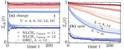
Figure 4: (a) ${\cal I}_{\text{ch}}(t)$ and (b) ${\cal I}_{\text{s}}(t)$ for $\ket{\psi_{2}(0)}$ at fixed $W=4$, $U=4$, and different lattice tilts $V\leq 16$. Data for chains with OBC and $L=8,12$ (dashed, solid) are compared to $L\to\infty$ NLCE dynamics with $c_{\text{max}}=11,12$ (squares, circles). NLCE remains well converged except for ${\cal I}_{\text{s}}(t)$ and $V=4$.

Next, we consider the initial state $\ket{\psi_{2}(0)}$ in Eq. (5) with ${\cal I}_{\text{ch}}(t)$ shown in Fig. 3 (b) for exemplary values of $W$. While we observe delocalized dynamics for $W=3$, most pronounced in case of the $L\to\infty$ NLCE data, ${\cal I}_{\text{ch}}(t)>0$ approaches approximately time-independent plateaus for $W=12,20$, suggesting charge localization at sufficiently strong disorder, cf. inset in Fig. 3 (c). While nonergodic charge dynamics has been observed before Prelovsek2016 ; Mondaini2015 , spin was found to be delocalized and relax subdiffusively instead Kozarzewski2018 . Here, we explore the fate of spin dynamics for $L\to\infty$ at strong disorder. Specifically, the spin imbalance ${\cal I}_{\text{s}}(t)$ is shown in Fig. 3 (c) for $W\leq 24$. Using NLCE up to $c_{\text{max}}=12$ Note_NLCE_Psi2 , we find no signatures of localization and ${\cal I}_{\text{s}}(t)$ decays as $\propto t^{-\alpha}$, $\alpha>0$ [inset in Fig. 3 (c)]. The fact that the $L\to\infty$ dynamics obtained by NLCE and for systems with $L=12$ agree very well with each other demonstrates that finite-size effects are negligible. Spin dynamics of ${\cal H}_{\text{FH}}$ thus behave delocalized even at extremely large $W$, where charge is frozen.

Dynamics in tilted lattice.– We now consider ${\cal H}_{\text{FH}}$ with $V>0$. While such tilts may lead to Stark localization Schulz2019 ; vanNieuwenburg2019 ; Guo2021 , nonergodic dynamics in strongly tilted lattices has also been attributed to Hilbert-space fragmentation Scherg2021 ; Khemani2020 ; Sala2020 ; Doggen2021 . Fixing the disorder to $W=4$ (for which ${\cal H}_{\text{FH}}$ is delocalized at $V=0$, cf. Fig. 3), Fig. 4 shows ${\cal I}_{\text{ch}}(t)$ and ${\cal I}_{\text{s}}(t)$ resulting from quenches with $\ket{\psi_{2}(0)}$ and different $V>0$, obtained by NLCE for $L\to\infty$ and direct simulations of finite chains with OBC. While $W>0$ is convenient to suppress the strong oscillations of ${\cal I}(t)$ SuppMat , the combination of disorder and lattice tilt may reinforce localization vanNieuwenburg2019 . Remarkably, we observe in Fig. 4 that not only ${\cal I}_{\text{ch}}(t)$ ceases to decay with increasing $V$, but ${\cal I}_{\text{s}}(t)$ also slows down drastically with $V$, especially compared to the case of bare disorder and no tilt [cf. Fig. 3 (c)]. In particular, for the largest $V=16$ considered here, ${\cal I}_{\text{s}}(t)$ does not substantially decay for $t<250$, suggesting the possibility to induce nonergodic spin dynamics on experimentally relevant time scales in tilted lattices. This is another key result. We stress that this mechanism of causing slow spin dynamics is distinct from other examples where localization was achieved by lifting the SU$(2)$ symmetry of ${\cal H}_{\text{FH}}$ Sroda2019 . While ${\cal I}_{\text{s}}(t)$ appears to be strongly initial-state dependent (see SuppMat ), we here leave it to future work to explore the effect of $V>0$ in more detail.

Conclusion.– To summarize, we have employed NLCE to study quantum quenches in disordered spin ladders and Fermi-Hubbard chains and obtained converged results for the imbalance ${\cal I}(t)$ on comparatively long time scales. We have put particular emphasis on intermediate disorder values $W<W_{\ast}$, where we demonstrated that NLCE outperform direct simulations of finite systems with OBC or PBC. Furthermore, in contrast to bare disorder, our analysis predicts that an additional tilted potential leads to a notable slowdown of spin dynamics for certain initial states in FH chains, which should be accessible experimentally Scherg2021 . Even though NLCE yield results for $L\to\infty$, allowing better estimates for $W_{\ast}$ Devakul2015 , we stress that, similar to other methods, an unambiguous detection of MBL is beyond its capabilities (and was not our goal). Since simulation times are limited, $t<\infty$, extracted values for $W_{\ast}$ should be understood as lower bounds for the putative MBL transition.

Given the apparent advantage of NLCE at intermediate disorder, a natural direction of research is to explore the emergence of subdiffusion on the ergodic side of the MBL transition Luitz2017 ; Weiner2019 ; Varma2017 ; Richter2018 . In this context, NLCE have been shown to be a powerful means to study transport properties of 1d systems in the thermodynamic limit Richter2019 . Another interesting avenue is to consider MBL in higher dimensions. While NLCE have proven competitive with other state-of-the-art methods to simulate quantum dynamics in 2d Richter2020_2 , reaching high expansion orders for 2d lattices is computationally demanding such that convergence times are still limited Gan2020 .

Acknowledgements.– This work was funded by the European Research Council (ERC) under the European Union’s Horizon 2020 research and innovation programme (Grant agreement No. 853368).

Supplemental material

I Numerical linked cluster expansion for disordered 1d systems

In addition to our explanations in the main text, let us provide further details on how to set up NLCE for disordered systems with inhomogeneous initial states, see also Gan2020S . The starting point is provided by a finite section of the infinite system, with a fixed disorder realization and initial state. As shown in Fig. S1 (a), one then selects a unit cell , which in our case is a single spin plaquette (in case of the spin ladder) or two neighboring lattice sites (in case of the Hubbard chain). While the imbalance ${\cal I}(t)$ is defined as a sum over the full system, the NLCE formalism relies on the calculation of the local unit-cell imbalance ${\cal I}_{\leavevmode\hbox to6.19pt{\vbox to2.8pt{\text{[drawing]}}}}(t)$, i.e., ${\cal I}(t)$ restricted to the chosen unit cell. As described in the main text, NLCE then consists of simulating finite clusters of increasing size and combining their contributions suitably. In Fig. S1 (b), we plot all clusters that have to be evaluated up to expansion order $c_{\text{max}}=4$, which means that the largest cluster in the expansion is of size $4\times 2$. In particular, for each cluster $c$ with a given size, all its translations ${\cal T}(c)$ shifted around the unit cell have to be evaluated. Note that for simulating the contributions of these clusters, the disorder realization and the respective alignment of the initial state has to remain fixed. Since the translations therefore contain different parts of the static disorder configuration, ${\cal I}_{\leavevmode\hbox to6.19pt{\vbox to2.8pt{\text{[drawing]}}}}(t)$ can vary for different translations. While NLCE by construction yields results in the thermodynamic $L\to\infty$, it is crucial to check the convergence of the series. Increasing $c_{\text{max}}$, i.e., including clusters with longer length scales, will typically increase the time scales on which the dynamics of ${\cal I}(t)$ remains converged.

As becomes apparent from Fig. S1 (b), the computational costs of employing NLCE up to some expansion order $c_{\text{max}}$ are notably higher than a direct simulation of a finite system with PBC or OBC of length $L=c_{\text{max}}$. In particular, while the latter requires the simulation of merely a single finite system (multiplied by the number of desired disorder samples), the former requires the simulation of multiple finite clusters within each expansion order, which is polynomially (roughly by a factor of $L$) more costly. As a consequence, we here restrict ourselves to expansion orders $c_{\text{max}}\lesssim 11$ [or $c_{\text{max}}\lesssim 12$ in case of Fermi-Hubbard chains with quarter-filling initial state $\ket{\psi_{2}(0)}$ in Eq. (5)]. While it is certainly possible to evaluate ${\cal I}(t)$ using sparse-matrix techniques on even larger clusters, NLCE simulations for this value of $c_{\text{max}}$ are already quite demanding and, in practice, yield converged results on sufficiently long time scales.

Eventually, as also mentioned in the main text, NLCE typically require disorder averaging over a larger number of samples to yield the same noise level as direct simulations of finite systems with PBC or OBC. This is caused by the fact that NLCE relies on the local evaluation of ${\cal I}_{\leavevmode\hbox to6.19pt{\vbox to2.8pt{\text{[drawing]}}}}(t)$ on the unit-cell, which is significantly smaller than the full system. In particular, while ${\cal I}_{\leavevmode\hbox to6.19pt{\vbox to2.8pt{\text{[drawing]}}}}(t)$ is in our case defined on $2$ or $4$ lattice sites (and is therefore most sensitive to the random fields/potentials on these sites), the imbalance ${\cal I}(t)$ in the case of finite $L$ is given by a sum over the full system, which leads to an effective disorder averaging over $\propto L$ local random fields/potentials.

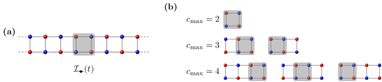
Figure S1: (a) NLCE provide a means to study the dynamics of the imbalance ${\cal I}(t)$ in the thermodynamic limit $L\to\infty$. To this end, consider an infinite ladder with inhomogeneous initial state (here Néel state as indicated by the red and blue lattice sites) and a fixed realization of disorder (not shown here). Next, identify a suitable unit cell to calculate the local unit-cell imbalance ${\cal I}_{-\bullet}(t)$ (here a plaquette of length $L=2$ with $2L=4$ lattice sites in total, as indicated by the shaded area). (b) ${\cal I}(t)$ in the thermodynamic limit is then obtained by suitably combining the contributions of clusters $c$ [and their translations ${\cal T}(c)$], which contain the unit cell (see Gan2020S and main text for details). For the quasi one-dimensional ladder, we consider only clusters that are ladders as well Richter2020_2S . All clusters that have to be evaluated up to expansion order $c_{\text{max}}=4$ are shown, where $c_{\text{max}}$ refers to the length of the largest cluster. Including larger and larger expansion orders leads to converged results of ${\cal I}(t)$ on longer time scales.

II Pure-state propagation

II.1 Chebyshev polynomial expansion

In order to access system (and cluster) sizes beyond the range of exact diagonalization (ED), we here subdivide the evolution up to time $t$ into a product of discrete time steps,

$$\ket{\psi(t)}=e^{-i{\cal H}t}\ket{\psi(0)}=\left(e^{-i{\cal H}\delta t}\right)^{Q}\ket{\psi(0)}\ ,$$ (S1)

where $\delta t=t/Q$. We approximate the action of the exponential $\exp(-i{\cal H}\delta t)$ by a Chebyshev-polynomial expansion Tal_Ezer_1984S ; Dobrovitski_2003S ; Fehske_2009S . Since the Chebyshev polynomials are defined on the interval $[-1,1]$, the spectrum of the original Hamiltonian ${\cal H}$ has to be rescaled Fehske_2009S ,

$$\widetilde{{\cal H}}=\frac{{\cal H}-b}{a}\ ,$$ (S2)

where $a$ and $b$ are suitably chosen parameters. In practice, we use the fact that the (absolute of the) extremal eigenvalue of ${\cal H}$ can be bounded from above Dobrovitski_2003S . For instance, in case of the disordered spin ladder ${\cal H}_{\text{SL}}$ we have,

$$\max(|E_{\text{min}}|,|E_{\text{max}}|)\leq\left(3N_{\langle\ell,m\rangle}/4+2WL/2\right)={\cal E}\ ,$$ (S3)

where $E_{\text{max}}$ ($E_{\text{min}}$) is the largest (smallest) eigenvalue of ${\cal H}_{\text{SL}}$, $N_{\langle\ell,m\rangle}=2(L-1)+L$ denotes the number of nearest-neighbor bonds (in the case of OBC), and the disorder $W$ couples to $2L$ operators $S_{\ell}^{z}$ with maximal eigenvalue $1/2$ each. Similar bounds for $E_{\text{max}}$ ($E_{\text{min}}$) can be obtained for disordered Hubbard chains ${\cal H}_{\text{FH}}$ as well. By choosing $a\geq{\cal E}$, it is guaranteed that the spectrum of ${\widetilde{\cal H}}$ lies within $[-1,1]$. As a consequence, we can set $b=0$. Note that while this choice of $a$ and $b$ is not necessarily optimal, it proves to be sufficient Dobrovitski_2003S .

Within the Chebyshev-polynomial formalism, the time evolution of a state $\ket{\psi(t)}$ can then be approximated as an expansion up to order $M$ Fehske_2009S ,

$$\ket{\psi(t+\delta t)}\approx c_{0}\ket{v_{0}}+\sum_{k=1}^{M}2c_{k}\ket{v_{k}}\ ,$$ (S4)

where the expansion coefficients $c_{0},c_{1},\dots,c_{M}$, are given by

$$c_{k}=(-i)^{k}{\cal J}_{k}(a\delta t)\ ,$$ (S5)

with ${\cal J}_{k}(a\delta t)$ being the $k$-th order Bessel function of the first kind evaluated at $a\delta t$. [Note that Eqs. (S4) and (S5) assume $b=0$.] Moreover, the vectors $\ket{v_{k}}$ are recursively generated according to

$$\ket{v_{k+1}}=2\widetilde{{\cal H}}\ket{v_{k}}-\ket{v_{k-1}}\ ,\ \quad k\geq 1\ ,$$ (S6)

with $\ket{v_{1}}=\widetilde{{\cal H}}\ket{v_{0}}$ and $\ket{v_{0}}=\ket{\psi(t)}$. Given a time step $\delta t$ (and the parameter $a$), the expansion order $M$ has to be chosen large enough to ensure negligible numerical errors.

As becomes apparent from Eqs. (S4) and (S6), the time evolution of the pure state $\ket{\psi(t)}$ requires the evaluation of matrix-vector products. Since ${\widetilde{\cal H}}$ is a sparse matrix, these matrix-vector multiplications can be implemented comparatively time and memory efficient. As a consequence, it is possible to treat system (or cluster) sizes that are larger compared to ED.

II.2 Accuracy of the time evolution

In Fig. S2 (a), the dynamics of the imbalance ${\cal I}(t)$ in a spin ladder of length $L=10$ with open boundary conditions is shown for $W=5$ and $W=15$, using a single realization of disorder in both cases. We compare data for different time steps $\delta t$ at fixed Chebyshev expansion order $M=25$. For all values of $\delta t$ considered here, we find that the resulting dynamics of ${\cal I}(t)$ is practically independent of $\delta t$ (note that for $W=15$, we only consider the smaller $\delta t=0.025,0.05$.). Focusing on $W=5$, Fig. S2 (b) furthermore shows results for a fixed time step $\delta t=0.1$ and varying values of $M$. While the data for $M=20$ and $M=25$ agree convincingly, deviations become apparent for the smaller $M=15$. In the inset of Fig. S2 (b), we additionally depict the norm $||\ket{\psi(t)}||^{2}=\braket{\psi(t)}{\psi(t)}$. For $M=20,25$, we find that $||\ket{\psi(t)}||$ remains essentially constant, $||\ket{\psi(t)}||=1$, for the entire time window considered here, whereas the conservation of $||\ket{\psi(t)}||$ is violated for $M=15$. In view of the data shown in Fig. S2, the numerical data presented in this paper are obtained using a time step $\delta t=0.1$ for low to intermediate disorder $W\leq 6$, while we choose $\delta t=0.05$ for larger $W$ (and sometimes even smaller $\delta t$ for large $W$ and $V$). We fix $M=25$. Using these parameters, we obtain accurate data on long time scales, which is crucial such that the NLCE remains well controlled when combining the contributions of multiple clusters.

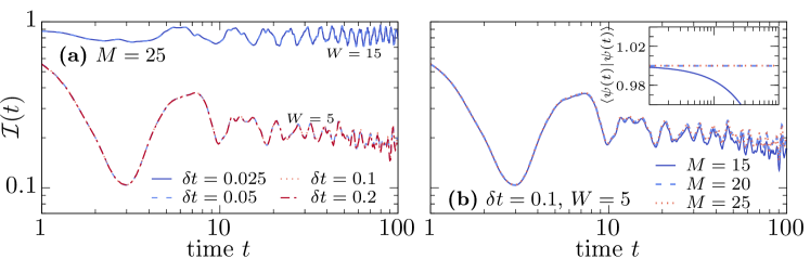
Figure S2: (a) Imbalace ${\cal I}(t)$ in spin ladders with OBC of length $L=10$ and disorder $W=5,15$. Data for different time steps $\delta t$ is compared at fixed Chebyshev expansion order $M=25$. (b) ${\cal I}(t)$ for $W=5$ using $\delta t=0.1$ and different choices of $M$. The inset shows the corresponding time dependence of the norm of $\ket{\psi(t)}$.

III Convergence of NLCE

As described in the main text, increasing the maximum cluster size $c_{\text{max}}$ will typically increase the time scales on which NLCE yield converged results. Focusing on ${\cal H}_{\text{SL}}$, Fig. S3 (a) shows ${\cal I}(t)$ for two different disorder strengths $W=3$ and $W=5$, obtained by NLCE for $c_{\text{max}}=7-11$. Moreover, we show data for finite systems with PBC or OBC of length $L=6,8,10$. Comparing the two values of $W$, we find that NLCE remain converged on longer time scales if disorder is stronger. In particular, while the curves for different $c_{\text{max}}$ agree convincingly with each other for $W=5$ up to the longest times $t\leq 200$ shown here, a breakdown of convergence can be clearly seen in the case of $W=3$ and smaller $c_{\text{max}}$. This observation can be understood by the fact that the dynamics become more and more localized for stronger disorder, i.e., the relevant length scales become shorter, such that clusters of smaller size are able to capture the dynamics in the thermodynamic limit. Importantly, while the NLCE data for $W=5$ are well converged for all $c_{\text{max}}$ shown here, the corresponding data of ${\cal I}(t)$ for finite systems with OBC or PBC in Fig. S3 (a) still show distinct finite-size effects. This is in line with our findings from the main text, i.e., for a given $c_{\text{max}}$ (corresponding to finite systems of length $L=c_{\text{max}}$), NLCE yield a better convergence than direct simulations of finite systems.

To gain more insights into the convergence properties of NLCE, let us define,

$$\delta[{\cal I}(t)]_{c_{\text{max}}}=|[{\cal I}(t)]_{c_{\text{max}}=11}-[{\cal I}(t)]_{c_{\text{max}}}|\ ,$$ (S7)

which is the difference between ${\cal I}(t)$ obtained by NLCE for some expansion order $c_{\text{max}}<11$ and ${\cal I}(t)$ obtained for the largest $c_{\text{max}}=11$ that is available to us. Focusing on $W=3$, Fig. S3 (b) shows $\delta[{\cal I}(t)]_{c_{\text{max}}}$ for $c_{\text{max}}=7-10$, as obtained from the data of ${\cal I}(t)$ in Fig. S3 (a). While $\delta[{\cal I}(t)]_{c_{\text{max}}}$ essentially vanishes at short times (i.e., the NLCE is well converged), we find that $\delta[{\cal I}(t)]_{c_{\text{max}}}$ grows with increasing time. While this indicates that the convergence of NLCE becomes worse at longer times, we find in Fig. S3 (b) that $\delta[{\cal I}(t)]_{c_{\text{max}}}$ systematically decreases with increasing $c_{\text{max}}$. In particular, as emphasized in the inset of Fig. S3 (b), $\delta[{\cal I}(t)]_{c_{\text{max}}}$ at fixed times $t=80,100,200$ decreases approximately exponentially with $c_{\text{max}}$. This demonstrates that the convergence of NLCE can be improved in a controlled way by including higher and higher expansion orders.

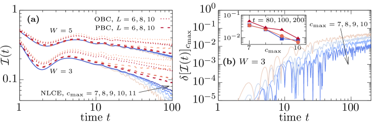
Figure S3: (a) Decay of the imbalance ${\cal I}(t)$ for ${\cal H}_{\text{SL}}$ with $W=3,5$, obtained by NLCE for expansion orders $c_{\text{max}}=7-11$. As a comparison, we show data obtained in finite systems with PBC and OBC and $L=6,8,10$. (b) Difference $\delta[{\cal I}(t)]_{c_{\text{max}}}$ between the dynamics of ${\cal I}(t)$ obtained for different expansion orders $c_{\text{max}}$ [cf. Eq. (S7)] at $W=3$. Inset: $\delta[{\cal I}(t)]_{c_{\text{max}}}$ at fixed times $t=80,100,200$ versus $c_{\text{max}}$.

IV Decay of imbalance in strongly disordered Hubbard chains

Let us present additional data for the decay of the charge imbalance ${\cal I}_{\text{ch}}(t)$ in Fermi-Hubbard chains ${\cal H}_{\text{FH}}$ at strong disorder. Focusing on the initial state $\ket{\psi_{1}(0)}$, Fig. S4 shows ${\cal I}_{\text{ch}}(t)$ obtained by NLCE for $c_{\text{max}}=9,10$ for varying disorder strengths $W\leq 10$. Similar to the case of the spin ladder considered in Fig. 2 in the main text, we find that ${\cal I}_{\text{ch}}(t)\propto t^{-\alpha}$ can be fitted by a power law at long times. In Fig. S4 (b), we plot $\alpha$ versus $W$. While $\alpha$ appears to approach zero for sufficiently strong $W$, the data in Fig. S4 (b) suggests that the critical disorder $W_{\ast}$ (for the half-filling sector probed by $\ket{\psi_{1}(0)}$) is probably even larger than the strongest value of $W$ considered here, $W_{\ast}\gtrsim 10$. Let us stress that this estimate is based on finite-time data $t<200$, such that we cannot make statements about the fate of charge localization in the limit $t\to\infty$ and the potential impact of the thermalizing spin dynamics [cf. Fig. 3 (c) in main text]. Moreover, we note that the extraction of $W_{\ast}$ can depend on the chosen initial state and its properties such as the density of doublons and singlons Protopopov2019S .

Figure S4: (a) Charge imbalance ${\cal I}_{\text{ch}}(t)$ in Fermi-Hubbard chains with initial state $\ket{\psi_{1}(0)}$ [Eq. (4)] and various disorder values $W$ (arrow), obtained by NLCE for expansion orders $c_{\text{max}}=9,10$. Shaded area indicates the standard error of the mean. (b) Power-law exponent $\alpha$ extracted from fits ${\cal I}_{\text{ch}}(t)\propto t^{-\alpha}$ [cf. dashed curves in panel (a)] in different time windows. We have $U=4$ in all cases.

V Additional data for decay of the spin imbalance in tilted Fermi-Hubbard chains

Let us present additional data for the dynamics of ${\cal I}_{\text{s}}(t)$ in Fermi-Hubbard chains with $V>0$. In contrast to Fig. 2 of the main text, where we considered the dynamics resulting from $\ket{\psi_{2}(0)}$ [cf. Eq. (5)], we now study two different initial states,

$$\ket{\psi_{3}(0)} =\prod_{\ell}c_{2\ell,\uparrow}^{\dagger}c_{2\ell+1,\downarrow}^{\dagger}\ket{0}=\left|\begin{array}[]{cccccc}\cdots&\uparrow&\downarrow&\uparrow&\downarrow&\cdots\end{array}\right\rangle\ ,$$ (S9)

$$\ket{\psi_{4}(0)} =\prod_{\ell}c_{4\ell,\uparrow}^{\dagger}c_{4\ell+1,\uparrow}^{\dagger}c_{4\ell+2,\downarrow}^{\dagger}c_{4\ell+3,\downarrow}^{\dagger}\ket{0}=\left|\begin{array}[]{cccccccccc}\cdots&\downarrow&\downarrow&\uparrow&\uparrow&\downarrow&\downarrow&\uparrow&\uparrow&\cdots\end{array}\right\rangle\ .$$ (S11)

In contrast to $\ket{\psi_{2}(0)}$, which has quarter-filling, $\ket{\psi_{3}(0)}$ and $\ket{\psi_{4}(0)}$ probe the dynamics in the half-filling sector. Taking the example of $\ket{\psi_{3}(0)}$ it is also insightful to write the spin imbalance ${\cal I}_{\text{s}}(t)$ as,

$${\cal I}_{\text{s}}(t)\propto\sum_{\ell}(-1)^{\ell}\langle(n_{\ell,\uparrow}-n_{\ell,\downarrow})(t)\rangle=\sum_{\ell=1}^{L}\langle(n_{\ell,\uparrow}-n_{\ell,\downarrow})(t)\rangle\langle(n_{\ell,\uparrow}-n_{\ell,\downarrow})(0)\rangle=\sum_{\ell=1}^{L}\langle m_{\ell}(t)\rangle\langle m_{\ell}(0)\rangle\ ,$$ (S12)

where we have rewritten ${\cal I}_{\text{s}}(t)$ as a correlation function and introduced the local magnetization $m_{\ell}=n_{\ell,\uparrow}-n_{\ell,\downarrow}$. We note that the imbalances ${\cal I}_{\text{ch}}(t)$ and ${\cal I}_{\text{s}}(t)$ considered in the main text for $\ket{\psi_{1}(0)}$ and $\ket{\psi_{2}(0)}$ can be written in the form of similar correlation functions as well.

In Figs. S5 (a) and (b), ${\cal I}_{\text{s}}(t)$ resulting from the initial states $\ket{\psi_{3}(0)}$ and $\ket{\psi_{4}(0)}$ is shown for fixed $U=W=4$ and varying lattice tilts $V$. While ${\cal I}_{\text{s}}(t)$ is found to decay towards zero in both cases, indicating delocalization of spin degrees of freedom even for strong lattice tilts $V=24$, we find that ${\cal I}_{\text{s}}(t)$ does depend notably on the initial state. In particular, in the case of $\ket{\psi_{4}(0)}$ [Fig. S5 (b)], the decay of ${\cal I}_{\text{s}}(t)$ is found to be less abrupt and can be further slowed down by increasing $V$. Both for $\ket{\psi_{3}(0)}$ and $\ket{\psi_{4}(0)}$, however, the dynamics of ${\cal I}_{\text{s}}(t)$ are distinctly faster compared to the example of $\ket{\psi_{2}(0)}$ considered in Fig. 4 in the main text.

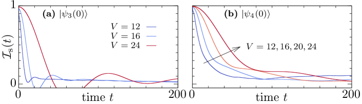
Figure S5: Spin imbalance in ${\cal H}_{\text{FH}}$ for different tilt strengths $V$, resulting from initial state (a) $\ket{\psi_{3}(0)}$ [Eq. (S9)] and (b) $\ket{\psi_{4}(0)}$ [Eq. (S11)]. Data are obtained for finite systems with $L=10$ and OBC. We have $U=4$ and $W=4$ in all cases.

VI Dynamics in the tilted Fermi-Hubbard chain without disorder

While we have considered the dynamics of ${\cal H}_{\text{FH}}$ in the main text for either $W>0$ at $V=0$ (Fig. $3$) or for $V>0$ at $W=4$ (Fig. $4$), let us here present additional data for the case of having just a tilted lattice without additional disorder, i.e., $V>0$ and $W=0$. In Figs. S6 (a) and (b), we show the charge and spin imbalances ${\cal I}_{\text{ch}}(t)$ and ${\cal I}_{\text{s}}(t)$ resulting from quenches with the initial state $\ket{\psi_{2}}$ [Eq. $(5)$ in main text] and different tilt values $V>0$. The data are obtained for finite systems with $L=12$ and open boundary conditions. To begin with, for $V=4$, we find that while ${\cal I}_{\text{ch}}(t\to\infty)>0$ saturates to a finite, approximately constant, long-time value, the spin imbalance ${\cal I}_{\text{s}}(t)$ clearly decays towards zero. For larger $V=8$ and $V=12$, in contrast, we find that spin dynamics clearly slow down as well. In particular, for $V=12$, we are unable to observe any notable decay of ${\cal I}_{\text{s}}(t)$ on the time scale $t\leq 250$ shown here. While the data in Fig. S6 is qualitatively similar to the data shown in Fig. 4 in the main text, we also note a number of differences. In particular, compared to the results of ${\cal I}_{\text{s}}(t)$ in Fig. 4 (b), spin dynamics in Fig. S6 (b) appears to be even more localized. This may potentially be understood due to the additional random disorder $W=4$ in Fig. 4, where due to rare configurations of the disorder $\epsilon_{\ell}$ at neighboring sites, the difference of the neighboring terms $\mu_{\ell}$ [cf. Eq. (3) in main text] becomes small such that the system behaves more ergodic. Moreover, in contrast to our results in Fig. 4, we now find that ${\cal I}_{\text{ch}}(t)$ and ${\cal I}_{\text{s}}(t)$ in Fig. S6 exhibit pronounced oscillations . These “Bloch oscillations” are expected in noninteracting models with tilted field, but survive to some extent in interacting models as well vanNieuwenburg2019S .

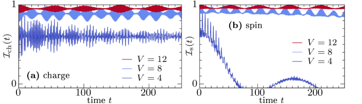
Figure S6: (a) Charge imbalance ${\cal I}_{\text{ch}}(t)$ in the Fermi-Hubbard model ${\cal H}_{\text{FH}}$ without disorder ($W=0$), resulting from quenches with the initial state $\ket{\psi_{2}}$ [see Eq. (5) in main text] and different lattice tilts $V=4,8,12$. Data are shown for chains with $L=12$ and open boundary conditions. (b) Analogous data, but now for the spin imbalance ${\cal I}_{\text{s}}(t)$.

VII Using NLCE to study localization dynamics in the disordered Heisenberg chain

While we have focused on disordered spin ladders and Fermi-Hubbard chains in the main text, the “standard” model to study the phenomenon of many-body localization is the disordered Heisenberg chain, described by the Hamiltonian,

$${\cal H}_{\text{Heis}}=\sum_{\ell=1}^{L}{\bf S}_{\ell}\cdot{\bf S}_{\ell+1}+\sum_{\ell=1}^{L}h_{\ell}S_{\ell}^{z}\ ,$$ (S13)

where the on-site fields $h_{\ell}\in[-W,W]$ are drawn at random, with $W$ setting the disorder strength.

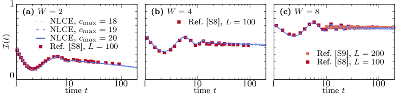
Figure S7: Imbalance ${\cal I}(t)$ in the disordered Heisenberg chain resulting from quenches with the antiferromagnetic initial state in Eq. (S14). NLCE results for expansion orders $c_{\text{max}}=20,19,18$ are compared to data obtained by matrix-product-state techniques from Ref. Doggen2018S ($L=100$) and Ref. Sierant2021S ($L=200$). Disorder is chosen as (a) $W=2$, (b) $W=4$, and (c) $W=8$. Our NLCE data are averaged over approximately $N_{s}\approx 2000$ disorder realizations.

It is straightforward to apply the NLCE approach discussed in the main part of this paper to study the nonequilibrium dynamics of ${\cal H}_{\text{Heis}}$. To this end, we here focus on the antiferromagnetic initial state,

$$\ket{\psi(0)}=\ket{\cdots\uparrow\downarrow\uparrow\downarrow\cdots}\ ,$$ (S14)

and consider the dynamics of the imbalance ${\cal I}(t)\propto\sum_{\ell}\langle S_{\ell}^{z}(t)\rangle\langle S_{\ell}^{z}(0)\rangle$. Including cluster sizes up to $c_{\text{max}}\leq 20$ (i.e., the largest clusters are chains of length $L=20$ with open boundaries), Figs. S7 (a), (b), and (c) show ${\cal I}(t)$ at $W=2$, $W=4$, and $W=8$, respectively. Considering the dynamics of ${\cal I}(t)$ up to times $t\leq 200$, we find that the NLCE is well-converged, i.e., the three different expansion orders $c_{\text{max}}=20,19,18$ shown in Fig. S7 essentially coincide with each other. Moreover, in order to benchmark our NLCE results, we also depict in Fig. S7 the digitized data of Ref. Doggen2018S and Ref. Sierant2021S , where ${\cal I}(t)$ was obtained using matrix-product-state (MPS) techniques. Generally, we find a convincing agreement between our NLCE results for $L\to\infty$ and the MPS data for $L=100,200$ in the literature.

References

- (1) R. Nandkishore and D. A. Huse, Annu. Rev. Condens. Matter Phys. 6, 15 (2015).
- (2) D. A. Abanin, E. Altman, I. Bloch, and M. Serbyn, Rev. Mod. Phys. 91, 021001 (2019).
- (3) I. V. Gornyi, A. D. Mirlin, and D. G. Polyakov, Phys. Rev. Lett. 95, 206603 (2005).
- (4) D. M. Basko, I. L. Aleiner, and B. L. Altshuler, Ann. Phys. 321, 1126 (2006).
- (5) V. Oganesyan and D. A. Huse, Phys. Rev. B 75, 155111 (2007).
- (6) A. Pal and D. A. Huse, Phys. Rev. B 82, 174411 (2010).
- (7) J. A. Kjäll, J. H. Bardarson, and F. Pollmann, Phys. Rev. Lett. 113, 107204 (2014).
- (8) J. Z. Imbrie, Phys. Rev. Lett. 117, 027201 (2016).
- (9) T. C. Berkelbach and D. R. Reichman, Phys. Rev. B 81, 224429 (2010).
- (10) D. J. Luitz, N. Laflorencie, and F. Alet, Phys. Rev. B 91, 081103(R) (2015).
- (11) S. Bera, H. Schomerus, F. Heidrich-Meisner, and J. H. Bardarson, Phys. Rev. Lett. 115, 046603 (2015).
- (12) L. D’Alessio, Y. Kafri, A. Polkovnikov, and M. Rigol, Adv. Phys. 65, 239 (2016).
- (13) B. Bauer and C. Nayak, J. Stat. Mech. 2013, P09005 (2013).
- (14) M. Žnidarič, T. Prosen, and P. Prelovšek, Phys. Rev. B 77, 064426 (2008).
- (15) J. H. Bardarson, F. Pollmann, and J. E. Moore, Phys. Rev. Lett. 109, 017202 (2012).
- (16) M. Serbyn, Z. Papić, and D. A. Abanin, Phys. Rev. Lett. 111, 127201 (2013).
- (17) D. A. Huse, R. Nandkishore, and V. Oganesyan, Phys. Rev. B 90, 174202 (2014).
- (18) A. Chandran, I. H. Kim, G. Vidal, D. A. Abanin, Phys. Rev. B 91, 085425 (2015).
- (19) V. Ros, M. Müller, and A. Scardicchio, Nucl. Phys. B 891, 420 (2015).
- (20) M. Schreiber, S. S. Hodgman, P. Bordia, H. P. Lüschen, M. H. Fischer, R. Vosk, E. Altman, U. Schneider, and I. Bloch, Science 349, 842 (2015).
- (21) J-y. Choi, S. Hild, J. Zeiher, P. Schauß, A. Rubio-Abadal, T. Yefsah, V. Khemani, D. A. Huse, I. Bloch, and C. Gross, Science 352, 1547 (2016).
- (22) J. Smith, A. Lee, P. Richerme, B. Neyenhuis, P. W. Hess, P. Hauke, M. Heyl, D. A. Huse, and C. Monroe, Nat. Phys. 12, 907 (2016).
- (23) D. J. Luitz and Y. Bar Lev, Ann. Phys. 529, 1600350 (2017).
- (24) T. Enss, F. Andraschko, and J. Sirker, Phys. Rev. B 95, 045121 (2017).
- (25) A. Nico-Katz, A. Bayat, and S. Bose, arXiv:2111.01146 (2021).
- (26) T. B. Wahl, A. Pal, S. H. Simon, Nat. Phys. 15, 164 (2019).
- (27) K. S. C. Decker, D. M. Kennes, and C. Karrasch, arXiv:2106.12861.
- (28) E. Chertkov, B. Villalonga, and B. K. Clark, Phys. Rev. Lett. 126, 180602 (2021).
- (29) A. C. Potter and R. Vasseur, Phys. Rev. B 94, 224206 (2016).
- (30) I. V. Protopopov, W. W. Ho, and D. A. Abanin, Phys. Rev. B 96, 041122(R) (2017).
- (31) S. A. Parameswaran and R. Vasseur, Rep. Prog. Phys. 81, 082501 (2018).
- (32) I. V. Protopopov, R. K. Panda, T. Parolini, A. Scardicchio, E. Demler, and D. A. Abanin, Phys. Rev. X 10, 011025 (2020).
- (33) R. M. Nandkishore and S. L. Sondhi, Phys. Rev. X 7, 041021 (2017).
- (34) N. Y. Yao, C. R. Laumann, S. Gopalakrishnan, M. Knap, M. Müller, E. A. Demler, and M. D. Lukin, Phys. Rev. Lett. 113, 243002 (2014).
- (35) A. L. Burin, Phys. Rev. B 91, 094202 (2015).
- (36) R. Modak and T. Nag, Phys. Rev. E 101, 052108 (2020).
- (37) J. Richter, N. Casper, W. Brenig, and R. Steinigeweg, Phys. Rev. B 100, 144423 (2019).
- (38) J. Richter, D. Schubert, and R. Steinigeweg, Phys. Rev. Research 2, 013130 (2020).
- (39) J. Schliemann, J. V. I. Costa, P. Wenk, and J. C. Egues, Phys. Rev. B 103, 174203 (2021).
- (40) T. Grover and M. P. A. Fisher, J. Stat. Mech. 2014, P10010 (2014).
- (41) M. Schiulaz and M. Müller, AIP Conference Proceedings 1610, 11 (2014).
- (42) N. Y. Yao, C. R. Laumann, J. I. Cirac, M. D. Lukin, and J. E. Moore, Phys. Rev. Lett. 117, 240601 (2016).
- (43) J. Sirker, Phys. Rev. B 99, 075162 (2019).
- (44) M. Schulz, C. A. Hooley, R. Moessner, and F. Pollmann, Phys. Rev. Lett. 122, 040606 (2019).
- (45) E. van Nieuwenburg, Y. Baum, and G. Refael, PNAS 116, 9269 (2019).
- (46) A. Smith, J. Knolle, D. L. Kovrizhin, and R. Moessner, Phys. Rev. Lett. 118, 266601 (2017).
- (47) M. Brenes, M. Dalmonte, M. Heyl, and A. Scardicchio, Phys. Rev. Lett. 120, 030601 (2018).
- (48) T. Heitmann, J. Richter, T. Dahm, and R. Steinigeweg, Phys. Rev. B 102, 045137 (2020).
- (49) P. Karpov, R. Verdel, Y.-P. Huang, M. Schmitt, and M. Heyl, Phys. Rev. Lett. 126, 130401 (2021).
- (50) S. Gopalakrishnan and S. A. Parameswaran, Phys. Rep. 862, 1 (2020).
- (51) A. Morningstar, L. Colmenarez, V. Khemani, D. J. Luitz, and D. A. Huse, arXiv:2107.05642.
- (52) W. De Roeck and F. Huveneers, Phys. Rev. B 95, 155129 (2017).
- (53) E. V. H. Doggen, I. V. Gornyi, A. D. Mirlin, and D. G. Polyakov, Phys. Rev. Lett. 125, 155701 (2020).
- (54) F. Weiner, F. Evers, and S. Bera, Phys. Rev. B 100, 104204 (2019).
- (55) R. K. Panda, A. Scardicchio, M. Schulz, S. R. Taylor, and M. Žnidarič, Europhys. Lett. 128, 67003 (2020).
- (56) P. Sierant and J. Zakrzewski, Phys. Rev. B 105, 224203 (2022).
- (57) E. V. H. Doggen, F. Schindler, K. S. Tikhonov, A. D. Mirlin, T. Neupert, D. G. Polyakov, and I. V. Gornyi, Phys. Rev. B 98, 174202 (2018).
- (58) D. A. Abanin, J. H. Bardarson, G. De Tomasi, S. Gopalakrishnan, V. Khemani, S. A. Parameswaran, F. Pollmann, A. C. Potter, M. Serbyn, and R. Vasseur, Ann. Phys. 427, 168415 (2021).
- (59) P. Sierant, M. Lewenstein, and J. Zakrzewski, Phys. Rev. Lett. 125, 156601 (2020).
- (60) J. Šuntajs, J. Bonča, T. Prosen, and L. Vidmar, Phys. Rev. E 102, 062144 (2020).
- (61) M. Kiefer-Emmanouilidis, R. Unanyan, M. Fleischhauer, and J. Sirker, Phys. Rev. Lett. 124, 243601 (2020).
- (62) D. Sels and A. Polkovnikov, Phys. Rev. E 104, 054105 (2021).
- (63) S. Paeckel, T. Köhler, A. Swoboda, S. R. Manmana, U. Schollwöck, and C. Hubig, Ann. Phys. 411, 167998 (2019).
- (64) H. Burau and M. Heyl, Phys. Rev. Lett. 127, 050601 (2021).
- (65) S. J. Thomson and M. Schiró, Phys. Rev. B 97, 060201(R) (2018).
- (66) T. K. Kvorning, L. Herviou, and J. H. Bardarson, arXiv:2105.11206.
- (67) D. M. Kennes, arXiv:1811.04126.
- (68) C. Hubig and J. I. Cirac, SciPost Phys. 6, 031 (2019).
- (69) A. Kshetrimayum, M. Goihl, and J. Eisert, Phys. Rev. B 102, 235132 (2020).
- (70) E. Baygan, S. P. Lim, and D. N. Sheng, Phys. Rev. B 92, 195153 (2015).
- (71) D. Wiater and J. Zakrzewski, Phys. Rev. B 98, 094202 (2018).
- (72) J. Hauschild, F. Heidrich-Meisner, and F. Pollmann, Phys. Rev. B 94, 161109(R) (2016).
- (73) P. Prelovšek, O. S. Barišić, and M. Žnidarič, Phys. Rev. B 94, 241104(R) (2016).
- (74) R. Mondaini and M. Rigol, Phys. Rev. A 92, 041601(R) (2015).
- (75) M. Kozarzewski, P. Prelovšek, and M. Mierzejewski, Phys. Rev. Lett. 120, 246602 (2018).
- (76) J. Zakrzewski and D. Delande, Phys. Rev. B 98, 014203 (2018).
- (77) T. Iadecola and M. Žnidarič, Phys. Rev. Lett. 123, 036403 (2019).
- (78) I. V. Protopopov and D. A. Abanin, Phys. Rev. B 99, 115111 (2019).
- (79) D. V. Kurlov, M. S. Bahovadinov, S. I. Matveenko, A. K. Fedorov, V. Gritsev, B. L. Altshuler, G. V. Shlyapnikov, arXiv:2112.06895.
- (80) Q. Guo, C. Cheng, H. Li, S. Xu, P. Zhang, Z. Wang, C. Song, W. Liu, W. Ren, H. Dong, R. Mondaini, and H. Wang, Phys. Rev. Lett. 127, 240502 (2021).
- (81) B. Tang, E. Khatami, and M. Rigol, Comput. Phys. Commun. 184, 557 (2013).
- (82) S. Scherg, T. Kohlert, P. Sala, F. Pollmann, B. H. Madhusudhana, I. Bloch, and M. Aidelsburger, Nat. Commun. 12, 4490 (2021).
- (83) E. Guardado-Sanchez, A. Morningstar, B. M. Spar, P. T. Brown, D. A. Huse, and W. S. Bakr, Phys. Rev. X 10, 011042 (2020).
- (84) R. Yao, T. Chanda, and J. Zakrzewski, Ann. Phys. 435, 168540 (2021).
- (85) J.-Y. Desaules, A. Hudomal, C. J. Turner, and Z. Papić, Phys. Rev. Lett. 126, 210601 (2021).
- (86) T. Prosen and M. Žnidarič, Phys. Rev. B 86, 125118 (2012).
- (87) S. Scherg, T. Kohlert, J. Herbrych, J. Stolpp, P. Bordia, U. Schneider, F. Heidrich-Meisner, I. Bloch, and M. Aidelsburger, Phys. Rev. Lett. 121, 130402 (2018).
- (88) For , and we focus on in this case.
- (89) S. Dusuel, M. Kamfor, K. P. Schmidt, R. Thomale, and J. Vidal, Phys. Rev. B 81, 064412 (2010).
- (90) M. Rigol, T. Bryant, and R. R. P. Singh, Phys. Rev. Lett. 97, 187202 (2006).
- (91) A. Biella, J. Jin, O. Viyuela, C. Ciuti, R. Fazio, and D. Rossini, Phys. Rev. B 97, 035103 (2018).
- (92) A. B. Kallin, K. Hyatt, R. R. P. Singh, and R. G. Melko, Phys. Rev. Lett. 110, 135702 (2013).
- (93) J. Richter and R. Steinigeweg, Phys. Rev. B 99, 094419 (2019).
- (94) J. Richter, F. Jin, L. Knipschild, H. De Raedt, K. Michielsen, J. Gemmer, and R. Steinigeweg, Phys. Rev. E 101, 062133 (2020).
- (95) T. Heitmann, J. Richter, J. Gemmer, and R. Steinigeweg, Phys. Rev. E 104, 054145 (2021).
- (96) I. G. White, B. Sundar, and K. R. A. Hazzard, arXiv:1710.07696.
- (97) B. Wouters, J. De Nardis, M. Brockmann, D. Fioretto, M. Rigol, and J.-S. Caux, Phys. Rev. Lett. 113, 117202 (2014).
- (98) K. Mallayya and M. Rigol, Phys. Rev. E 95, 033302 (2017)
- (99) K. Mallayya and M. Rigol, Phys. Rev. Lett. 120, 070603 (2018).
- (100) E. Guardado-Sanchez, P. T. Brown, D. Mitra, T. Devakul, D. A. Huse, P. Schauß, and W. S. Bakr, Phys. Rev. X 8, 021069 (2018).
- (101) J. Richter, T. Heitmann, and R. Steinigeweg, SciPost Phys. 9, 031 (2020).
- (102) B. Tang, D. Iyer, and M. Rigol, Phys. Rev. B 91, 161109(R) (2015).
- (103) M. D. Mulanix, D. Almada, and E. Khatami, Phys. Rev. B 99, 205113 (2019).
- (104) J. Park and E. Khatami, Phys. Rev. B 104, 165102 (2021).
- (105) T. Devakul and R. R. P. Singh, Phys. Rev. Lett. 115, 187201 (2015).
- (106) J. Gan and K. R. A. Hazzard, Phys. Rev. A 102, 013318 (2020).
- (107) See supplemental material for details on numerical linked cluster expansions for disordered systems, the forward propagation of pure states using Chebyshev polynomials, the convergence properties and the accuracy of NLCE, as well as additional numerical results, including a comparison of NLCE and matrix-product state simulations in the disordered 1d Heisenberg model.
- (108) Note that for ladders, more complicated cluster shapes are in principle conceivable. In practice, it turns out that for such (quasi-)1d geometries, fully connected clusters yield a convincing convergence of the NLCE Mallayya2018 ; Richter2020_2 .
- (109) K. Bhattaram and E. Khatami, Phys. Rev. E 100, 013305 (2019).
- (110) R. Schäfer, I. Hagymási, R. Moessner, and D. J. Luitz, Phys. Rev. B 102, 054408 (2020).
- (111) H. Tal-Ezer and R. Kosloff, J. Chem. Phys. 81, 3967 (1984).
- (112) V. V. Dobrovitski and H. De Raedt, Phys. Rev. E 67, 056702 (2003).
- (113) H. Fehske, J. Schleede, G. Schubert, G. Wellein, V. S. Filinov and A. R. Bishop, Phys. Lett. A 373, 2182 (2009).
- (114) We calculate as , where denotes the imbalance for a single disorder realization and is the number of disorder samples.
- (115) Since is in the quarter-filling sector, which has a lower Hilbert-space dimension, the computational costs are reduced such that we consider slightly larger .
- (116) V. Khemani, M. Hermele, and R. Nandkishore, Phys. Rev. B 101, 174204 (2020).
- (117) P. Sala, T. Rakovszky, R. Verresen, M. Knap, and F. Pollmann, Phys. Rev. X 10, 011047 (2020).
- (118) E. V. H. Doggen, I. V. Gorny, and D. G. Polyakov, Phys. Rev. B 103, L100202 (2021).
- (119) M. Środa, P. Prelovšek, and M. Mierzejewski, Phys. Rev. B 99, 121110(R) (2019).
- (120) V. K. Varma, A. Lerose, F. Pietracaprina, J. Goold, and A. Scardicchio, J. Stat. Mech. (2017), 053101 (2017).
- (121) J. Richter, J. Herbrych, and R. Steinigeweg, Phys. Rev. B 98, 134302 (2018).

References

- (1) J. Gan and K. R. A. Hazzard, Phys. Rev. A 102, 013318 (2020).
- (2) J. Richter, T. Heitmann, and R. Steinigeweg, SciPost Phys. 9, 031 (2020).
- (3) H. Tal-Ezer and R. Kosloff, J. Chem. Phys. 81, 3967 (1984).
- (4) V. V. Dobrovitski and H. De Raedt, Phys. Rev. E 67, 056702 (2003).
- (5) H. Fehske, J. Schleede, G. Schubert, G. Wellein, V. S. Filinov and A. R. Bishop, Phys. Lett. A 373, 2182 (2009).
- (6) I. V. Protopopov and D. A. Abanin, Phys. Rev. B 99, 115111 (2019).
- (7) E. van Nieuwenburg, Y. Baum, and G. Refael, PNAS 116, 9269 (2019).
- (8) E. V. H. Doggen, F. Schindler, K. S. Tikhonov, A. D. Mirlin, T. Neupert, D. G. Polyakov, and I. V. Gornyi, Phys. Rev. B 98, 174202 (2018).
- (9) P. Sierant and J. Zakrzewski, arXiv:2109.13608.