Chandra - BAT

Chandra Follow-up Observations of Swift-BAT-selected AGNs II

Abstract

We present the combined Chandra and Swift-BAT spectral analysis of nine low-redshift ($z\leq 0.10$), candidate heavily obscured active galactic nuclei (AGN) selected from the Swift-BAT 150-month catalog. We located soft (1$-$10 keV) X-ray counterparts to these BAT sources and joint fit their spectra with physically motivated models. The spectral analysis in the 1$-$150 keV energy band determined that all sources are obscured, with a line-of-sight column density N${}_{H}\geq$ 10²² cm^-2 at a 90% confidence level. Four of these sources show significant obscuration with N${}_{H}\geq$ 10²³ cm^-2 and two additional sources are candidate Compton-thick Active Galactic Nuclei (CT-AGNs) with N${}_{H}\geq$ 10²⁴ cm^-2. These two sources, 2MASX J02051994-0233055 and IRAS 11058$-$1131, are the latest addition to the previous 3 CT-AGN candidates found using our strategy for soft X-ray follow-up of BAT sources. In here we present the results of our methodology so far, and analyze the effectiveness of applying different selection criteria to discover CT-AGN in the local Universe. Our selection criteria has a $\sim$20% success rate of discovering heavily obscured AGN whose CT nature is confirmed by follow-up NuSTAR observations. This is much higher than the $\sim$5% found in blind surveys.

1 Introduction

Current models have concluded the Cosmic X-ray Background (CXB), the diffuse X-ray emission in the 1 to $\sim$200$-$300 keV band, is primarily produced by accreting supermassive black holes (SMBHs), i.e., active galactic nuclei (AGNs, Alexander et al., 2003; Gandhi & Fabian, 2003; Gilli et al., 2007; Treister et al., 2009; Ueda et al., 2014). While the CXB emission below 10 keV has been almost entirely resolved (Worsley et al., 2005; Hickox & Markevitch, 2006), at $\sim$30 keV (the peak of the CXB, Ajello et al., 2008), only 30% of the emission is accounted for by current observations (Aird et al., 2015; Civano et al., 2015; Mullaney et al., 2015; Harrison et al., 2016). It is expected that a considerable fraction (10-20%) of the CXB is produced by a numerous population of heavily obscured, the so-called Compton thick (CT-) AGN, which have intrinsic obscuring hydrogen column densities (N_H) $\geq$ 10²⁴ cm^-2 (Risaliti et al., 1999; Alexander et al., 2003; Gandhi & Fabian, 2003; Gilli et al., 2007; Treister et al., 2009; Ueda et al., 2014; Ananna et al., 2019). However, only 5$-$7% of the hard X-ray detected low-$z$ AGNs are classified as CT-AGNs (Comastri, 2004; Della Ceca et al., 2008; Burlon et al., 2011; Ricci et al., 2015; Lanzuisi et al., 2018) which is much lower than those predicted by population synthesis models that aim to explain the CXB (30$-$50%; see, e.g., Gilli et al., 2007; Ueda et al., 2014; Ananna et al., 2019). Currently, there are only $\sim$30-35 NuSTAR-confirmed CT-AGN in the range $z\leq 0.05$ (Torres-Albà et al., 2021). The low number severely limits any science designed to study this population. Detecting new CT-AGN in X-rays is crucial to advance the field, in order to explain the shape of the CXB, and to study torus properties via complex models.
The emission from CT-AGNs is heavily suppressed below 10 keV due to the heavy obscuration of the dusty gas surrounding the SMBH, which makes detecting CT-AGN in X-rays difficult. Their spectra is dominated by the Compton hump at $\sim$20$-$40 keV, originating from the intrinsic emission being reflected in the torus.

Several models developed over the past decade successfully describe the X-ray emission of AGN reprocessed by the torus material, e.g., pexrav (Magdziarz & Zdziarski, 1995); MYTorus (Murphy & Yaqoob, 2009; Yaqoob, 2012); BNtorus (Brightman & Nandra, 2011); ctorus (Liu & Li, 2014); borus02 (Baloković et al., 2018); UXClumpy (Buchner et al., 2019); XClumpy (Tanimoto et al., 2019). These models are built adopting different assumptions on the geometrical distribution of the obscuring material (e.g., homogeneous vs clumpy) or its chemical composition. The clumpy models are significant because numerous works have observed variability in the line-of-sight column density, suggesting that a patchy, non-homogeneous distribution of obscuring material is favored by observational data (Risaliti et al., 2002; Bianchi et al., 2012; Torricelli-Ciamponi et al., 2014). However, implementing these models requires high-quality data in order to break the various degeneracies between parameters. It is thus necessary to increase our pool X-ray CT-AGN, which let the reflection component shine through thanks to the suppressed line-of-sight. Previous works have used high-quality X-ray data to successfully constrain torus parameters (e.g. Zhao et al., 2020).
Instruments such as the Swift X-Ray Telescope (Swift-XRT) on board the Neil Gehrels Swift satellite (Gehrels et al., 2004), Chandra, and XMM-Newton, sensitive in the $\sim$0.3$-$10 keV energy range, can only detect the Compton hump if the source’s spectrum is largely redshifted ($z>1$). In the local universe ($z<0.1$), an instrument with sensitivity above 10 keV is necessary to detect and characterize CT-AGNs (e.g., Marchesi et al., 2017a). The wide-field (120$\times$90 deg²) Burst Alert Telescope (Barthelmy et al., 2005) continually observes the whole sky in the 15$-$200 keV band. Swift-BAT is thus an excellent tool to create a census of the hard X-ray emitting sources in the local universe. The combination of Swift-BAT and soft X-ray instruments has previously proved successful in selecting and identifying candidate CT-AGNs (Burlon et al., 2011; Vasudevan et al., 2013; Ricci et al., 2015; Koss et al., 2016; Marchesi et al., 2017a, b).
In this work, we perform a joint Chandra–Swift-BAT spectral fitting in the 1.0$-$150 keV band of nine AGN detected by Swift-BAT in 150 months of observations. The joint analysis of Chandra and Swift-BAT data provides an ample opportunity to constrain the column density of the obscuring material surrounding the accreting SMBHs and possibly identify new candidate CT-AGNs. The aim of this work is therefore to obtain a first estimate of the line-of-sight column density for these sources, which have never been observed before in soft X-rays. Thanks to this estimate, obtained via our quick snapshot Chandra program (PI: Marchesi, see Section 2), we find promising targets to follow-up with joint NuSTAR and XMM-Newton observations. This program will allow to obtain new high-quality data of promising CT-AGN candidates to confirm their nature, which will add to the limited pool of high-quality CT-AGNs that can be used to constrain torus properties (e.g. Zhao et al., 2020) and CXB models (e.g. Ananna et al., 2019). The second objective of this work is to present the results of our program so far, and discuss the efficiency of the selection criteria we have used to target new CT-AGN in the local Universe.
In addition, Chandra’s unparalleled spatial resolution ($\sim$0.5$\arcsec$) allows us to detect X-ray emission extended out to kiloparsec scales. Recent works have discovered CT-AGN with extended emission in the 3-7 keV band primarily aligned with the ionization cones, but also present in the orthogonal direction (the cross-cones; see e.g., Fabbiano et al., 2017, 2018; Jones et al., 2020; Ma et al., 2020; Jones et al., 2021). The study of the extended emission in CT-AGN has the power to constrain the duty cycle for the AGN feedback onto the host galaxy ISM (Ma et al., 2020).

This work is organized as follows: Section 2 describes the selection criteria used to identify potential CT-AGN candidates and the data reduction process. Section 3 discusses the models used in our spectral fitting and Section 4 describes the derived results. Section 5 reports the findings on the extended emission. Section 6 summarizes the conclusions and future work. All errors reported are at a 90% confidence level. Standard cosmological parameters are as follows: H₀ = 70 km s^-1 Mpc^-1, q₀ = 0.0, and $\Lambda$ = 0.73.

2 Selection Criteria and Data Reduction

Since its launch, Swift-BAT has continuously observed the hard X-ray sky. Data from the first 150 months have been combined into a catalog containing sources detected with fluxes down to $f\sim$ 3.3$\times$10^-12 erg s^-1 cm^-2 in the 15$-$150 keV band (Segreto et al. in preparation). Due to its high sensitivity and ability to cover the entire sky, Swift-BAT provides an excellent tool to study the hard X-ray AGN population in the nearby Universe.
The Swift-BAT data are processed by the BAT_IMAGER code (Segreto et al., 2010). This code was developed to analyze data from coded mask instruments and can perform screening, mosaicking, and source detection. All spectra used in this work have been background subtracted and were acquired by averaging over the entire Swift-BAT exposure. The standard BAT spectral redistribution matrix was used.
The sample in this work is selected from the 150 month catalog, which includes a total of 724 galaxies in the local (z $<$ 0.10, D $\lesssim$ 400 Mpc) Universe. The first step in our three-step program is to select previously unobserved sources within these 724 to propose for quick ($\sim 10$ ks) Chandra observations. In order to find promising CT-AGN candidates, we implement the following criteria:

• We select sources at high Galactic latitude ($\lvert b\rvert>$ 10$\degree$) without a ROSAT (Voges et al., 1999) counterpart. The emission in the 0.1 $-$ 2.4 keV band, in which ROSAT is sensitive, is easily suppressed in heavily obscured AGN and the lack of this counterpart already suggests an expected column density logN${}_{H}>$ 23 (Ajello et al., 2008; Koss et al., 2016). The added requirement of high Galactic latitude ensures that the obscuration responsible for the lack of ROSAT counterpart is not coming from our own galaxy.

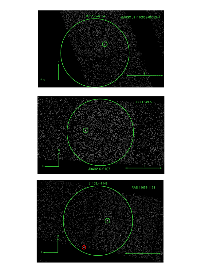
Figure 9: From top to bottom: the Chandra exposures for 2MASX J11110059$-$0053347, ESO 549$-$50, IRAS 11058$-$1131 in the 1$-$7 keV range. Large green circles represent the BAT 95 % uncertainty region while small green circles identify the correct counterpart of the BAT source; red/magenta circles are for sources detected by Chandra and located within/nearby the BAT 95 % uncertainty region, but which we determine are not the counterparts of the BAT source (see the text for more details).

• We only select Seyfert 2 galaxies (Sy2s) or sources classified as galaxies. The absence of broad lines in Sy2s implies the presence of obscuring material in our line of sight. This is significant as $\sim$95% of Seyfert 2 galaxies are obscured with a column density logN${}_{H}>$ 22 (Figure 9, Koss et al., 2017). Sources optically classified as galaxies are likewise likely to be potentially obscured AGN. This is because a normal galaxy cannot emit strongly enough in the $15-150$ keV range to be detected by BAT, and must therefore be an AGN. Any AGN that is optically not classified as such is likely to be obscured. We note that our nine sources have optical spectra available and lack typical AGN features, hence they are likely obscured.

• Finally, this sample is limited to sources in the nearby universe because CT-AGN are detected at much lower redshifts than the rest of the AGN population (Burlon et al., 2011). Approximately 90% of the Swift-BAT-detected CT-AGN have been discovered at $z$ $\leq$ 0.1, while unobscured or Compton-thin AGN can be found up to z$\sim$0.3 (Ricci et al., 2017).

The above selection criteria have proved capable of discovering heavily obscured AGN candidates in the past, as described in Marchesi et al. (2017a). The last nine sources for which we obtained Chandra observing time following the described criteria are analysed in this work, and listed in Table 1.

All sources were observed with 10 ks by Chandra ACIS-S as a part of the Chandra general observing Cycles 19 and 21 (Proposal numbers 19700430 and 21700085, P.I. Marchesi ). The CIAO (Fruscione et al., 2006) 4.12 software was used to reduce the data following standard procedures. Source and background spectra were extracted utilizing the CIAO specextract tool. Source spectra were calculated with a 5$\arcsec$ radius, while background spectra used an annulus with internal radius r_in = 6$\arcsec$ and external radius r_out = 15$\arcsec$. Background annuli experienced no contamination from nearby sources. We applied point-source aperture correction as a part of the source spectral extraction process. We fit the spectra using Cstat, given how the low count statistic of our sources does not allow the minimum 15 cts/bin required to use $\chi^{2}$ statistics (for all except MCG $+$08-33-046). To bin the spectra, we followed Lanzuisi et al. (2013) (Appendix A), which study the optimal binning to use C-statistic (cstat) as a fitting statistic. They find that fitting is stable regardless of binning at either 1 or 5 cts/bin, but 5 cts/bin results in the optimal error determination. Therefore, we adopt this value except in two cases: ESO 090$-$IG 014 and IRAS 11058$-$1131. Due to the low net counts ($<$90 cts) of these two sources, 5 cts/bin resulted in the dilution of visible features, such as the iron line, which affected the fit negatively. For these two sources, we opted for a 3 cts/bin; the value that is closest to 5 without erasing the iron line.

Table 1: Summary of Sources in Our Sample

Swift-BAT ID	Source Name	R.A.	Decl.	$z$	Exp. Time	Count Rate	Obs Date	Type
		(J2000)	(J2000)		(ks)	(1–7 keV)
J0205.2$-$0232	2MASX J02051994$-$0233055∗	02:05:19.9	$-$02:33:05.9	0.0283	9.9	4.40e-2	2018 June 11	Ga
J0402.6$-$2107	ESO 549$-$50†	04:02:46.1	$-$21:07:08.6	0.0252	9.9	1.55e-2	2019 Nov 23	Sy2b
J0407.8$-$6116	2MASX J04075215$-$6116126∗	04:07:52.1	$-$61:16:12.8	0.0214	10.4	1.58e-2	2018 May 05	Ga
J0844.8$+$3055	2MASX J08445829$+$3056386∗	08:44:58.3	+30:56:38.3	0.0643	9.9	1.15e-1	2018 Jan 03	AGNb
J0901.8$-$6418	ESO 090$-$IG 014∗	09:01:37.2	$-$64:16:28.1	0.0220	9.9	8.29e-3	2018 June 01	IGc
J1108.4$-$1148	IRAS 11058$-$1131†	11:08:20.3	$-$11:48:12.1	0.0548	9.7	3.83e-3	2020 Mar 2	Sy2b
J1111.0$+$0054	2MASX J11110059$-$0053347†	11:11:00.6	$-$00:53:34.9	0.0908	9.9	4.61e-2	2020 May 12	Sy2b
J1258.4$+$7624	IRAS 12571$+$7643†	12:58:36.0	+76:26:41.3	0.0634	9.9	1.95e-2	2020 Jan 22	Ga
J1828.8$+$5021	MCG $+$08-33-046†	18:28:48.1	+50:22:20.9	0.0169	9.9	1.90e-1	2020 Jan 24	Sy2b

Notes:
$*$: From the 100-month BAT Catalog.
$\dagger$: From the 150-month BAT Catalog.
a: Galaxy. Paturel et al. (2003)
b: Seyfert 2 Galaxy. Véron-Cetty & Véron (2006)
c: Interacting Galaxy. Arp & Madore (1987)

3 Spectral Analysis Results

Spectral fitting was conducted with XSPEC v. 12.10.1f (Arnaud, 1996). The Heasoft tool nh (Kalberla et al., 2005) was used to calculate Galactic absorption in the direction of each source. The flux and intrinsic luminosity for each source were calculated using clumin in xspec. The tables listing the results of the 1$-$7 keV spectral fitting of the nine Swift-BAT galaxies are reported in the Appendix. In this section, we introduce the models that are used to analyze the source spectra in $\S$3.1 and the fitting results in $\S$4.

3.1 Models Implemented

3.1.1 MYTorus

The MYTorus (Murphy & Yaqoob, 2009) model assumes a uniform torus of absorbing material with circular cross section and a fixed opening angle of 60$\arcdeg$. The model is composed of three components: the line-of-sight continuum, the Compton-scattered component (i.e. reflection), and the fluorescent lines. The line-of-sight continuum, also described as the zeroth-order continuum, is the intrinsic X-ray emission from the AGN as observed after absorption from the surrounding torus. Next, the Compton-scattered component models the photons that scatter into the observer line of sight after interacting with the dust and gas surrounding the SMBH. In the case the true covering factor of the source differs from the default MYTorus value, $f_{c}=cos(\theta)=$ 0.5, or a not negligible time delay exists between the intrinsic emission and the scattered component, the two components require different normalizations. The normalization for the scattered component is denoted as $A_{S}$ (Yaqoob, 2012). The final component models the most significant fluorescent lines, i.e., the Fe K$\alpha$ and Fe K$\beta$ lines, at 6.4 and 7.06 keV, respectively. This component also has its own normalization, $A_{L}$. $A_{S}$ and $A_{L}$ were fixed to 1 due to the low quality of our spectra. In our analysis, we also searched for the presence of a thermal component below 1 keV, which is observed in the X-ray spectra of AGN. However, due to the low count statistic of our spectra at soft X-ray energies, none of our fits was significantly improved when adding a thermal component (mekal).
In XSPEC notation, our model is defined as:

$$ModelA=constant_{1}*phabs*(MYTZ*$$

$$zpowerlw+A_{S}*MYTS+A_{L}*MYTL$$

$$+f_{s}*zpowerlw),$$ (1)

where $MYTZ*zpowerlw$ represents the line-of-sight continuum (or the zeroth-order continuum), $MYTS$ the scattered component, and $MYTL$ the fluorescent lines. Lastly, $f_{s}$ is the fraction of intrinsic emission that leaks through the torus rather than being absorbed by the obscuring material. The MYTorus model can be utilized in two different configurations, designated ‘coupled’ and ‘decoupled’ (Yaqoob, 2012).

3.1.2 MYTorus in Coupled Configuration

MYTorus measures the angle between the axis of the torus and the observer line of sight, known as the torus inclination angle, which will hereafter be written as $\theta_{obs}$. This angle ranges from 0$\arcdeg-$90$\arcdeg$, where $\theta_{obs}$ = 90$\arcdeg$ represents edge-on observing and $\theta_{obs}$ = 0$\arcdeg$ represents face-on observing. When MYTorus is in the coupled configuration, all three components of the model are set to have the same $\theta_{obs}$, which is a free parameter, and the same column density.

3.1.3 MYTorus in Decoupled Configuration

The decoupled configuration of MYTorus was initially introduced in Yaqoob (2012) and adds the flexibility of allowing different values for the line-of-sight column density, $N_{H,Z}$, and the average torus column density, $N_{H,S}$; a first approximation to a clumpy distribution. In this configuration, the line-of-sight continuum is fixed to an angle of $\theta_{obs,Z}$ = 90$\arcdeg$. The scattered and fluorescent line components have an equal $\theta_{obs,S,L}$, which can either be fixed to 90$\arcdeg$ or 0$\arcdeg$ to represent edge-on or face-on reflection, respectively. In the edge-on reflection scenario, the obscuring material between the AGN and the observer reprocesses the photons. In the face-on reflection scenario, the emission reflecting off the far side of the torus passes through and is observed (which could also be a sign of a patchy distribution of material). In MYTorus decoupled, the scattered and fluorescent line column densities are represented by $N_{H,S}$, which can vary greatly from the line-of-sight column density in an inhomogeneous, patchy torus.

3.1.4 BORUS02

The second physically motivated model we used to analyze our data is borus02 (Baloković et al., 2018). This model incorporates an absorbed intrinsic continuum multiplied by a line-of-sight absorbing component, zphabs $\times$ cabs. Additionally, borus02 models the reprocessed component, including the Compton-scattered component and fluorescent lines. This model includes the torus covering factor as a free parameter which varies in the range from $f_{c}$ = 0.1$-$1, equivalent to a torus opening angle $\theta_{tor}$ = 0$\arcdeg-$84$\arcdeg$. borus02 is implemented in XSPEC in the following way:

$$ModelB=constant_{1}*phabs*$$ (2)

$$(borus02+zphabs*cabs*zpowerlw$$

$$+f_{s}*zpowerlaw),$$

where $borus02$ models the reprocessed components, which includes the scattered continuum and fluorescent line emission. In addition, borus02 includes the high-energy cutoff and iron abundance as free parameters. We froze the energy cutoff at 500 keV to remain consistent with the default setting in MYTorus and fixed the iron abundance to 1 due to low statistics in our data. The zphabs and cabs components account for the line-of-sight absorption within the source, including Compton scattering losses out of the line of sight.

4 Results

In Figure 1, we report the borus02 best-fit line-of-sight column density as a function of redshift for the nine objects presented in this paper, as well as for those obtained in previous works by our group. The subsequent subsections describe the fitting results for all nine sources. For every source, we removed from the BAT spectra those data points with error bars compatible with a non-detection. We note that in the tables of best-fit parameters for the final five sources, we only list the Chandra cstat/dof as the BAT data showed poor fitting statistics, likely due to the large intrinsic dispersion. For example, the BAT data for 2MASX J11110059$-$0053347 had only 10 points yet was responsible for $\sim$90% of the reduced statistic.
We note that we compared our errors from the model fits with errors calculated using a Markov Chain Monte Carlo (MCMC) algorithm. As both methods produced similar results, we are confident the errors derived from the models are valid.
In the Appendix, we show the analysed Chandra images of each source, along with the corresponding BAT positional uncertainty region at a 95% confidence level. In each image, the counterpart listed in Table 1 is marked within the BAT region. The region size is calculated by

$$R_{95}(\arcmin)=12.5\times[S/N]^{-0.68}+0.54,$$ (3)

where S/N is the significance of the detection (see Cusumano et al., 2010; Segreto et al., 2010, for details). The size of this region for each source can be found in Table 12. For the majority of our sources, there is only one object within the BAT region, making it the clear counterpart. In cases where it is not as clear, further discussion can be found below, in the respective subsection detailing the analysis of each object.
We note that the Chandra and BAT data are not taken simultaneously, as BAT gives an average of the spectrum over 150 months of observation. This implies our observations are susceptible to being affected by variability. Any non-CT variability in the line-of-sight column density does not have an impact in our analysis, given how BAT is sensitive to emission $>15$ keV, an energy range unaffected by line-of-sight obscuration. However, flux variability between the two observations can occur, and therefore we have included a Chandra cross-normalization constant, C_cha, to account for this. It is possible that extreme flux variability can occur, causing our models to mistakenly classify a source as highly obscured when it is only in a low-flux state. We note that this has not happened before and our previous works show that the Chandra$-$BAT analysis produces reasonably accurate column density measurements (however with large uncertainties) when compared with the XMM-Newton$-$NuSTAR results (Marchesi et al., 2017a; Zhao et al., 2019a, b). This is why any of our sources that are compatible with $N_{H}>10^{24}$ cm^-2 must be considered only a candidate CT-AGN until simultaneous XMM-Newton and NuSTAR observations can verify the classification.

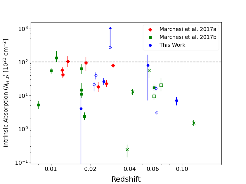
Figure 1: The line-of-sight column density as a function of redshift. The blue circles represent the borus02 best fit line-of-sight column densities from the nine sources in the work, the red diamonds represent the seven sources analyzed in Marchesi et al. (2017a) with a fixed inclination angle of 90$\arcdeg$, and the green squares represent the results from Marchesi et al. (2017b). Unfilled shapes are reported as galaxies in SIMBAD (see Table 1). The four X symbols are Seyfert 1 galaxies. Sources above the dashed line are candidate Compton-thick AGNs (i.e., having line-of-sight column density N_H,Z $\geq$ 10²⁴ cm^-2). The arrow pointed upwards represents a source with only a lower limit on the line-of-sight N_H,Z.

4.1 X-ray Spectral Fitting Results

4.1.1 ESO 090$-$IG 014

As is visible in Figure 2, there are 2 other X-ray sources in the Chandra field, 2MASS J09015969$-$6416408 (red) and WISEA J090129.46$-$641551.1 (magenta) that are within or near ($<1\arcmin$) the BAT 95% confidence region (R $\approx$ 3$\arcmin$). Neither source has any X-ray emission above 3 keV. Furthermore, ESO 090$-$IG 014 (green) is $\sim$3 magnitudes brighter in the WISE W3 band, the band most commonly associated with AGN emission (Asmus et al., 2015). For these reasons, it is highly unlikely that either of the other two sources would contribute to the Swift-BAT data.
The best fit results are displayed in Table 2. All four models show good agreement with a soft photon index $\Gamma\approx$ 2.20. ESO 090$-$IG 014 is one of the sources for which the best fit required a cross-normalization not equal to 1, C${}_{cha}\approx 0.3$, suggesting that the Chandra observation was taken in a low-flux epoch. Except MYTorus coupled, all models suggest an obscured AGN with $N_{H,Z}\approx 4\times 10^{23}$ cm^-2. The average torus column density is lower, on the order of 10²² cm^-2, suggesting a clumpy torus. In the borus02 model, the covering factor and $\theta_{obs}$ were fixed to 0.5 and 87$\arcdeg$ (the upper limit in borus02), respectively, since the data quality was not high enough to properly constrain them (as suggested by Zhao et al., 2020). We note these values are consistent with the poorly-constrained best-fit values. Also, $f_{s}$ is frozen to zero in borus02, given how the best-fit results yields $f_{s}$ $<$ 10^-5, compatible with zero.

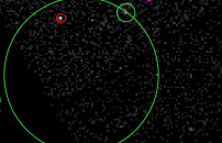
Figure 2: The Chandra CCD for the 10 ks of ESO 090$-$IG 014 (marked with the smaller of the two green circles) in the 1$-$7 keV range. Two other nearby sources, 2MASS J09015969$-$6416408 (red) and WISEA J090129.46$-$641551.1 (magenta), were studied and are believed to have not contributed to the BAT emission (see the text for further details). The large green circle (2.87$\arcmin$ in radius, see Table 12) represents the 95% Swift-BAT confidence region.

Table 2: ESO 090$-$IG 014

Model	MYTorus	MYTorus	MYTorus	borus02
	(Coupled)	(Decoupled Face-on)	(Decoupled Edge-on)
cstat/dof	43/27	42/27	42/27	40/27
$\Gamma$	2.19${}^{+0.17}_{-0.18}$	2.17${}^{+0.17}_{-0.17}$	2.21${}^{+0.16}_{-0.17}$	2.12${}^{+0.16}_{-0.18}$
$N_{H,eq}$	1.35${}^{+1.90}_{-1.03}$	…	…	…
norm $10^{-2}$	0.42${}^{+0.09}_{-0.07}$	0.50${}^{+0.14}_{-0.09}$	0.60${}^{+0.08}_{-0.06}$	0.44${}^{+0.02}_{-0.02}$
cf,Tor	…	…	…	0.5*
cos($\theta_{obs}$)	0.49${}^{+}_{-0.01}$	…	…	0.05*
$N_{H,Z}$	…	0.37${}^{+0.12}_{-0.10}$	0.42${}^{+0.16}_{-0.08}$	0.40${}^{+0.10}_{-0.09}$
$N_{H,S}$	…	0.01${}^{+0.25}_{-}$	0.03${}^{-}_{-}$	0.01${}^{+0.23}_{-}$
$f_{s}$ 10-2	0.20${}^{+0.23}_{-0.17}$	0.24${}^{+0.33}_{-}$	0.07${}^{+0.26}_{-}$	0*
Ccha	0.34${}^{+0.21}_{-0.14}$	0.30${}^{+0.17}_{-0.11}$	0.32${}^{+0.20}_{-0.17}$	0.34${}^{+0.20}_{-0.06}$
L$\rm{}_{2-10\,keV}$				1.02${}^{+0.24}_{-0.19}$ $\times$ 1043
L$\rm{}_{15-55\,keV}$				6.46${}^{+0.62}_{-0.57}$ $\times$ 1042

Notes:
*: Parameter was frozen to this value during fitting.
${}^{-}_{-}$: Parameter is unconstrained.
$\Gamma$: Power law photon index.
N_H,eq: Hydrogen column density along the equator of the torus in units of 10²⁴ cm^-2.
norm: the main power-law normalization (in units of photons cm² s^-1 keV^-1 $\times$ 10^-4), measured at 1 keV.
c_f,Tor: Covering factor of the torus.
cos($\theta_{obs}$): Cosine of the inclination angle.
$N_{H,Z}$: Line-of-sight torus hydrogen column density, in units of 10²⁴ cm^-2.
$N_{H,S}$: Average torus hydrogen column density, in units of 10²⁴ cm^-2.
$f_{s}$: Fraction of scattered continuum.
C_cha: The cross-normalization constant between the Chandra and Swift-BAT data.
L$\rm{}_{2-10\,keV}$: Intrinsic luminosity in the 2$-$10 keV band with units of erg s^-1.
L$\rm{}_{15-55\,keV}$: Intrinsic luminosity in the 15$-$55 keV band with units of erg s^-1.

4.1.2 2MASX J02051994$-$0233055

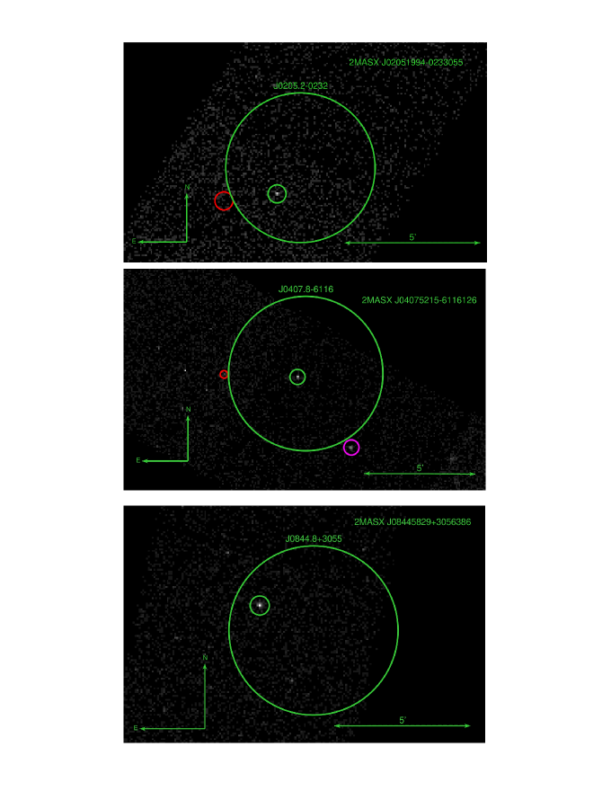
Figure 8: From top to bottom: the Chandra exposures for 2MASX J02051994$-$0233055, 2MASX J04075215$-$6116126, 2MASX J08445829$+$3056386 in the 1$-$7 keV range. Large green circles represent the BAT 95 % uncertainty region while small green circles identify the correct counterpart of the BAT source; red/magenta circles are for sources detected by Chandra and located within/nearby the BAT 95 % uncertainty region, but which we determine are not the counterparts of the BAT source (see the text for more details).

The 150-month catalog lists 2MASX J02051994$-$0233055 (green in Figure 8) as the counterpart of the BAT emission. The 105-Month Swift-BAT catalog (Oh et al., 2018), however, includes a BAT source that overlaps with the one studied here, with WISEA J020527.94$-$023321.8 (red) listed as its counterpart. We mark the position of both possible counterparts in the Chandra field image in Appendix B, showing that there is no Chandra emission coming from WISEA J020527.94$-$023321.8. Moreover, WISEA J020527.94$-$023321.8 is $\sim$4 magnitudes dimmer in the W3 band. The counterpart of the BAT emission is thus 2MASX J02051994$-$0233055.

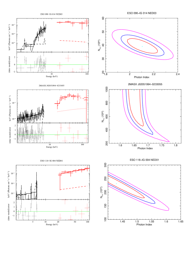
Figure 5: Unfolded Chandra (black) and BAT (red) spectrum of each source fitted with the borus02 model. The best-fitting line-of-sight component is plotted as a solid line, while the reflection component is a dashed line and the scattered component is a dotted line. The confidence contours at 68%, 90%, and 99% are displayed for $\Gamma$ and N_H,Z (in units of 10²² cm^-2).

While the majority of the models for 2MASX J02051994$-$0233055 are in agreement, the MYTorus decoupled edge-on configuration yielded significantly different results in the line-of-sight column density (8.6${}^{+4.0}_{-2.5}$ $\times$ 10²³ cm^-2). The other three models suggest a heavily CT-AGN with line-of-sight column density N${}_{H,Z}>>$ 10²⁴ cm^-2. According to the borus02 model results, displayed in Figure 5, the spectrum is reflection dominated.
We tested the reliability of the reflection-dominated scenario using the pexmon model as follows:

$$ModelC=constant*phabs*(zphabs*zpowerlw+$$ (4)

$$pexmon+f_{s}*zpowerlw).$$

pexmon is a neutral Compton reflection model with self-consistent Fe and Ni lines (George & Fabian, 1991; Nandra et al., 2007). It includes a scaling factor, R, which allows to consider (R = 1) or exclude (R $<$ 0) the intrinsic emission component. We opt for the latter, as the inclusion of zphabs*zpowerlaw allows to estimate the line of sight column density. The best fit line-of-sight column density for the pexmon model is N_H,Z = 5.54${}^{+5.76}_{-3.44}$ $\times$ 10²⁴ cm^-2.
Finally, we also attempt to model the source using the MYTorus decoupled model in a combination of both face-on and edge-on configurations. This model is consistent with the MYTorus coupled, MYTorus decoupled face-on, and borus02 results, with best-fit estimations all suggesting line-of-sight and average column densities on the order of 10²⁵ cm^-2. Based on the results derived from all models, we believe 2MASX J02051994$-$0233055 to be a reliable CT-AGN candidate.

4.1.3 2MASX J04075215$-$6116126

ESO 118$-$IG 004 (red in Figure 8) was originally listed as the most reliable counterpart for 4PBC J0407.8$-$6116 as it is bright in the W3 band ($\sim$7.5). However, the analysis of the Chandra data allowed us to challenge this claim, and determine that 2MASX J04075215$-$6116126 (green) is the true source of the BAT emission. As seen in Appendix B, 2MASX J04075215$-$6116126 is at the center of the BAT 95% confidence region, while ESO 118$-$IG 004 is located just outside of it. Also, 2MASX J04075215$-$6116126 has a count rate (in the 2$-$10 keV band) more than 15 times greater than that of ESO 118$-$IG 004. Furthermore, ESO 118$-$IG 004 shows a flux decay toward higher energies, while 2MASX J04075215$-$6116126 shows an increase consistent with a Compton-thin source. However, it is not impossible that ESO 118$-$IG 004 is a highly CT source that contributes in a non-negligible way to the BAT flux. For this reason, we have been awarded NuSTAR + XMM simultaneous observations to study these sources and verify their column densities.
We note that the source WISEA J040732.53$-$611918.3 (magenta) is also present in the Chandra image, located just outside of the BAT confidence region. However, it is $\sim$5 times dimmer in X-rays and $\sim$3 magnitudes dimmer in the W3 band. Therefore, we do not believe it contributes to the BAT flux.
The four models used agree on most parameters. All estimate a photon index $\Gamma\approx$ 1.60 with only 7% errors and a line-of-sight column density around 2.0$\times$10²³ cm^-2. The reflection component parameters are less tightly constrained due the fact that, in this particular source, reflection is subdominant. The average torus column density is similar to the line-of-sight value, $\approx$ 2.0$\times$10²³ cm^-2, however with uncertainties greater than half an order of magnitude. The borus02 model yields a value of 0.90 for both the covering factor and the cosine of the inclination angle although largely unconstrained.

4.1.4 2MASX J08445829$+$3056386

2MASX J08445829$+$3056386 was also detected in the 105-Month BAT catalog under the counterpart name FBQS J084458.3+305638.
In this work, all four models are in good agreement with most parameters, including an average AGN photon index of $\Gamma\approx$ 1.75. The two MYTorus decoupled models and borus02 suggest this is a Compton-thin AGN with an N_H,Z of the order of 10²² cm^-2. This result is consistent with the fact that the source has a high count rate, 0.115 ct s^-1, which would be unusual for a Swift-BAT-detected CT-AGN at $z\sim 0.07$. The borus02 model cannot constrain $\theta_{obs}$, so it was fixed to cos($\theta_{obs}$) = 0.05. In addition, the scattering constant $f_{s}$ is also fixed to zero due to its best-fit result being compatible with zero, i.e., $f_{s}<$ 10^-5.

4.1.5 2MASX J11110059$-$0053347

All four models displayed in Table 7 show consistent N_H,Z values $\sim$ 7$\times$10²² cm^-2, signaling a Compton-thin AGN. The photon index was well constrained around $\Gamma$=1.65 with $\sim$5% errors. As evidenced by the low obscuration measured for this source, we conclude the intrinsic emission dominates over the reflection component. Therefore, we were unable to provide any constraint on the torus parameters derived from the reflection component such as the average torus column density, the inclination angle, and the covering factor.

4.1.6 ESO 549$-$50

All models yielded a well-constrained average photon index of $\Gamma\approx$ 1.85 with only 10% uncertainties. Moreover, the four best-fit results are in agreement with an N_H,Z $\approx$ 3$\times$10²³ cm^-2, indicating this source is significantly obscured. While the covering factor appears to be well constrained around 0.35, neither the inclination angle nor the average torus column density are. The average torus column density is only loosely constrained (N${}_{H,tor}>$ 10²³).

4.1.7 IRAS 11058$-$1131

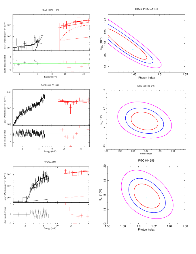
Figure 7: Unfolded Chandra (black) and BAT (red) spectrum of each source fitted with the borus02 model. The best-fitting line-of-sight component is plotted as a solid line, while the reflection component is a dashed line and the scattered component is a dotted line. The confidence contours at 68%, 90%, and 99% are displayed for $\Gamma$ and N_H,Z (in units of 10²² cm^-2).

The Chandra image in Appendix B shows IRAS 11058$-$1131 surrounded by several hot pixels, as well as the source 2MASS J11083339$-$1151500 (red in Figure 9) near the bottom of the BAT region. Upon further inspection, it was revealed the latter does not have emission above 3 keV and is $\sim$ 4 magnitudes fainter in the WISE W3 band. Thus, is unlikely to be the true BAT counterpart.
As can be seen in Figure 7, this source has a significant drop-off in flux in the Chandra data compared to the BAT data. For this reason, we let the Chandra cross-normalization constant, $C_{cha}$, free to vary and fixed the BAT constant to 1. Most of the models have a $C_{cha}$ value $<1$, although with large uncertainties. IRAS 11058$-$1131 is best-fit with a high N_H,Z value as exemplified by the large decrease in the soft-energy band. These values range from Compton-thin, 8$\times$10²³ cm^-2, to CT, 2.6$\times$10²⁴ cm^-2. Since both of these results are statistically equivalent, we list IRAS 11058$-$1131 as a CT-AGN candidate. The average torus column density shows better agreement among the three applicable models with values in the CT regime. The photon index is rather hard, averaging $\Gamma\sim$1.43.

4.1.8 MCG $+$08-33-046

The Chandra observation of MCG $+$08-33-046 is significantly affected by pile-up (over 20% according to the Chandra pileup tool, Davis, 2001). Considering this tool is only applicable to a power law, we were unable to utilize the models discussed in Section 3.1. With the pileup tool implemented, the best-fit has a photon index $\Gamma\sim$2 and an N_H,Z $\approx$ 2$\times$10²² cm^-2. This low line-of-sight column density agrees well with the high flux levels of this source in the soft X-rays.

4.1.9 IRAS 12571$+$7643

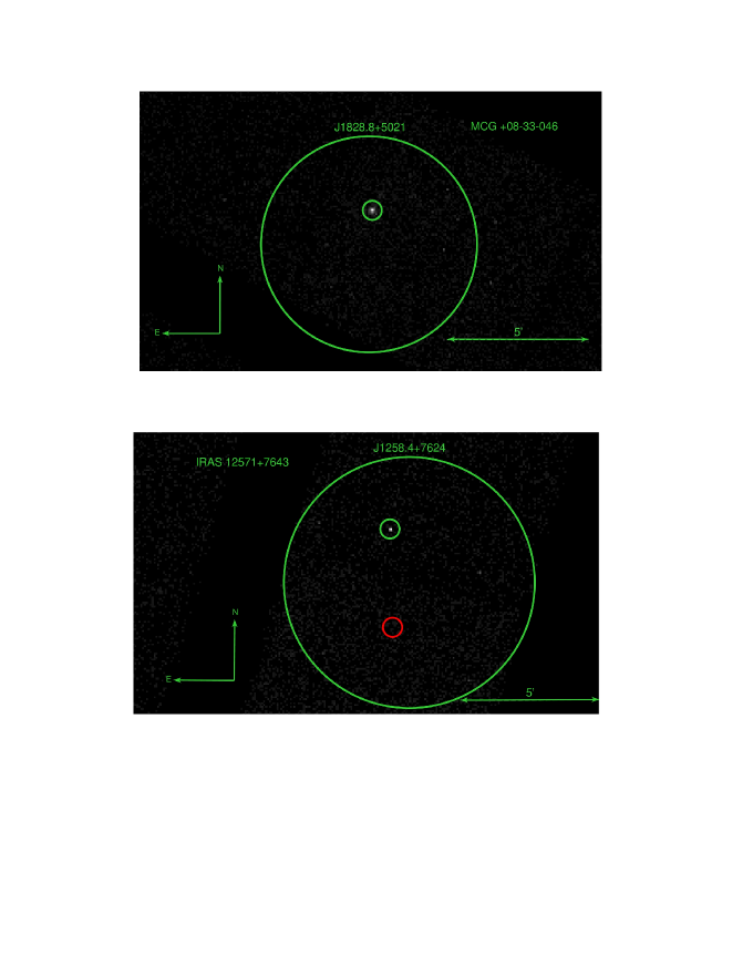
Figure 10: From top to bottom: the Chandra exposures for MCG $+$08-33-046, IRAS 12571$+$7643 in the 1$-$7 keV range. Large green circles represent the BAT 95 % uncertainty region while small green circles identify the correct counterpart of the BAT source; red/magenta circles are for sources detected by Chandra and located within/nearby the BAT 95 % uncertainty region, but which we determine are not the counterparts of the BAT source (see the text for more details).

We originally assumed PGC 044558 (red Figure 10) as the most likely counterpart of the BAT source, due to its Sy2 nature. However, there is no emission from this source in the Chandra exposure. As there is significant emission from IRAS 12571+7643 (green), which is also within the BAT 95% confidence region, we believe this is the true source of the BAT emission.
This is another Compton-thin candidate, with N_H,Z $\approx$ 1.7$\times$10²³ cm^-2. Most fits yielded an average column density on the order of 10²² cm^-2, significantly less than the line-of-sight N_H. This is only the third source in this sample to have N_H,Z $>$ N_H,S. The photon index was consistently around $\Gamma\sim$1.7 with $<$ 8% uncertainties.

4.2 Mid-IR Comparison

The Mid-infrared (MIR) is another useful waveband to select CT-AGN candidates. As the ultraviolet (UV) emission from the accretion disk gets absorbed by the dusty torus, it becomes heated to temperatures of several hundred Kelvins. As a result, the dust radiates thermally, with its emission peaking in the MIR ($\sim$3 - 30 $\mu$m, Asmus et al., 2020). As this emission is much less susceptible to absorption, many works have used the MIR to identify heavily obscured AGN (Yan et al., 2019; Asmus et al., 2020; Kilerci Eser et al., 2020; Guo et al., 2021). Moreover, Asmus et al. (2015) used a sample of 152 AGN with reliable soft X-ray data to model a trend between the intrinsic 2$-$10 keV luminosity and the 12$\mu$m luminosity (see Figure 3). In addition, we have plotted the intrinsic (closed circles) and observed (open circles) X-ray luminosities of the sources in this work, and those of recently confirmed CT-AGN (Marchesi et al., 2019; Zhao et al., 2019a, b; Torres-Albà et al., 2021; Traina et al., 2021). The two green stars represent the candidate CT-AGN presented in this work, 2MASX J02051994$-$0233055 and IRAS 11058$-$1131. It can be seen, 2MASX J02051994$-$0233055 shows a significant decrease from intrinsic to observed luminosity and IRAS 11058$-$1131 has an observed luminosity near the CT region. Both are strong indicators of a CT-AGN.

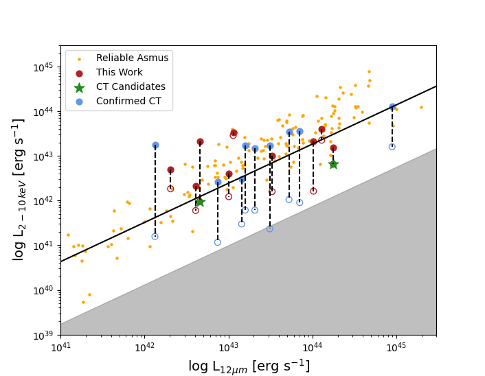
Figure 3: The 2$-$10 keV vs 12$\mu$m luminosities of the nine sources in this work. The filled circles represent the intrinsic 2$-$10 keV luminosities, while the open circles represent the observed luminosities. The green stars are the two candidate CT-AGN presented in this work, 2MASX J02051994$-$0233055 and IRAS 11058$-$1131. The black line is the relation derived from the X-ray observations of a reliable sample of 152 AGN presented in Asmus et al. (2015). The blue circles are recently confirmed CT-AGN (Marchesi et al., 2019; Zhao et al., 2019a, b; Torres-Albà et al., 2021; Traina et al., 2021). The grey area represents a 25$\times$ (or more) decrease in X-ray flux, a diagnostic used to identify CT-AGN (Annuar et al., 2020). The 12$\mu$m data were obtained by WISE.

5 Study of Extended Emission

The radiation from the accretion disk of an AGN is collimated by the torus, given how it is symmetric around the accretion flow axis. The radiation escaping from the AGN excites the gas of the interstellar medium (ISM) by photoionization, which appears in the form of cones extending from the nucleus. These cones have been observed in local Seyfert galaxies in NIR and optical (e.g. Durré & Mould, 2018), as well as X-rays (Fabbiano et al., 2017, 2018; Jones et al., 2020; Ma et al., 2020). In X-rays, the mentioned works have used Chandra’s unmatched resolution to observe kiloparsec-scale diffuse emission in both the hard continuum (3$-$7 keV) and in the Fe-K$\alpha$ line. Obscured, and particularly CT-AGN, are ideal to observe this extended X-ray emission given how the torus dims the much brighter nuclear emission.
We take advantage of our high-resolution Chandra images and attempt to detect the cone emission in the highly obscured sources presented in this work. In order to do so, we extract radial profiles from all of our sources and compare them to the expected radial profile of a point source of the same flux and in the same position. We follow the CIAO Point-Source Functions (PSF) simulation thread and generate the Chandra PSFs using ChaRT and MARX 5.5.1. Figure 4 shows a comparison between a simulated PSF and the observed emission, for the case of 2MASX J11110059$-$0053347. The two curves are compatible with each other, and there is no significant excess over the the simulated data counts. All sources in our sample show similar curves, and thus no sign of extended X-ray emission. 2MASX J11110059$-$0053347 has a count rate twice as high as the 10 ks exposure of MKN 573, a CT-AGN source analyzed in (Jones et al., 2021), which presents significant extended emission. Therefore, the ionization cone in the sources of our sample is either much fainter, or not present.

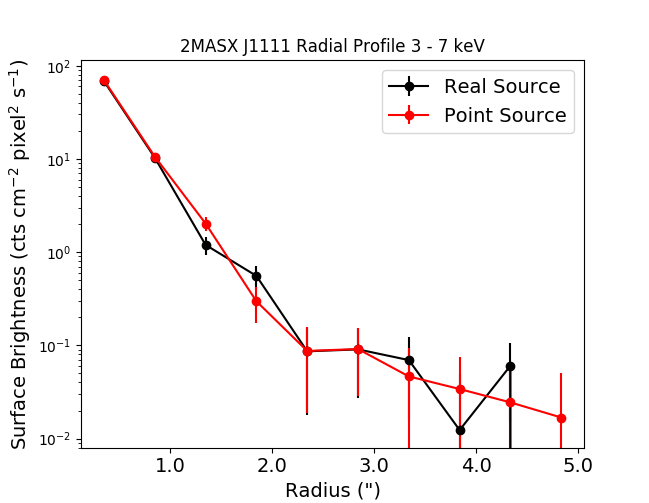
Figure 4: The 3$-7$ keV radial profile of 2MASX J11110059$-$0053347 compared to that of a simulated point source. The two curves are compatible, and therefore there is no significant evidence of extended emission. A similar trend exists for the other eight sources in this paper.

6 Discussion and Conclusions

In this paper, we presented the joint Chandra–Swift-BAT spectral fitting analysis in the 1$-$150 keV energy range for nine nearby ($z<$ 0.1) AGN selected from the 150-month Swift-BAT all-sky survey catalog. This represents the second step of our three step plan to discover new Compton-thick AGN in the local Universe. Our first step was selecting these sources following previous successful selection criteria (Marchesi et al., 2017a, and see Sect. 2) and acquiring Chandra snapshot observations for each of them. The third and final step will involve obtaining and analyzing XMM-Newton and NuSTAR observations of the best CT-AGN candidates found in this work. We identified these candidates by fitting the Swift-BAT and Chandra spectra with several models in order to constrain spectral parameters such as the intrinsic absorption, N_H,Z, and photon index, $\Gamma$, to uncover highly obscured AGN. The borus02 best-fit parameters for each source are listed in Table 3.

Table 3: Results for the Entire Sample

Source	ESO 090	2MASX J0205	2MASX J0407	2MASX J0844	2MASX J1111	ESO 549	IRAS 110	MCG $+$08	IRAS 125
cstat/dof	40/27	57/72	57/31	201/170	98/74	21/23	11/6	86/77	41/30
$\Gamma$	2.12${}^{+0.16}_{-0.18}$	1.65${}^{+0.09}_{-0.22}$	1.56${}^{+0.09}_{-0.14}$	1.74${}^{+0.07}_{-0.06}$	1.77${}^{+0.02}_{-0.19}$	1.91${}^{+0.02}_{-0.02}$	1.45${}^{+0.35}_{-}$	2.05	1.61${}^{+0.18}_{-0.07}$
$N_{H,eq}$	…	…	…	…	…	…	..	0.02	…
norm $10^{-2}$	0.44${}^{+0.02}_{-0.02}$	0.27${}^{+1.23}_{-0.16}$	0.04${}^{+0.02}_{-0.01}$	0.09${}^{+0.01}_{-0.01}$	0.06${}^{+0.02}_{-0.01}$	0.10${}^{+0.10}_{-0.02}$	0.04${}^{+0.16}_{-0.02}$	0.32	0.05${}^{+0.02}_{-0.01}$
cf,Tor	0.5*	0.87${}^{+0.11}_{-0.46}$	0.90${}^{-}_{-0.85}$	1.00${}^{-0.65}_{-}$	0.89${}^{-}_{-}$	0.35${}^{+0.05}_{-0.05}$	0.60${}^{-}_{-}$	…	0.15${}^{-}_{-}$
cos($\theta_{obs}$)	0.05*	0.78${}^{+0.21}_{-0.51}$	0.90${}^{-}_{-}$	0.05*	0.89${}^{-}_{-}$	0.95${}^{-}_{-0.77}$	0.05*	…	0.90${}^{-}_{-}$
$N_{H,Z}$	0.40${}^{+0.10}_{-0.09}$$\dagger$	10.00*$\dagger$	0.21${}^{+0.04}_{-0.08}$	0.030 ${}^{+0.003}_{-0.003}$$\dagger$	0.07${}^{+0.02}_{-0.02}$	0.26${}^{+0.08}_{-0.06}$	0.81${}^{+0.84}_{-0.74}$	…	0.16${}^{+0.05}_{-0.03}$
$N_{H,S}$	0.01${}^{+0.23}_{-}$	10.00${}^{-}_{-6.45}$	0.19${}^{+2.32}_{-0.15}$	0.24${}^{+0.22}_{-0.15}$	31.62${}^{-}_{-}$	14.13${}^{-}_{-}$	7.41${}^{-}_{-}$	…	0.01${}^{-}_{-}$
$f_{s}$ 10-2	0*	4.08${}^{+11.90}_{-2.63}$	2.03*	0*	0.03${}^{+0.04}_{-0.03}$	0*	0.03${}^{-}_{-}$	…	0.01${}^{+0.01}_{-}$
Ccha	0.34${}^{+0.20}_{-0.06}$	1*	1*	1*	1*	1*	0.70${}^{+5.30}_{-0.69}$	1*	1*
L$\rm{}_{2-10\,keV}$	1.02 $\times$ 1043	1.10 $\times$ 1042	1.51 $\times$ 1042	3.31 $\times$ 1043	3.98 $\times$ 1043	3.98 $\times$ 1042	1.55 $\times$ 1043	4.90 $\times$ 1042	2.09 $\times$ 1043
L$\rm{}_{15-55\,keV}$	6.46 $\times$ 1042	3.98 $\times$ 1042	3.16 $\times$ 1042	3.89 $\times$ 1043	5.01 $\times$ 1043	3.72 $\times$ 1042	3.16 $\times$ 1043	3.55 $\times$ 1042	3.63 $\times$ 1043

Notes: Same as Table 2.
$\dagger$: At least one of the models has a significantly different best-fit $N_{H,Z}$ value.

6.1 Model Comparison

The two configurations of MYTorus decoupled, face-on and edge-on, and borus02 were capable of satisfactorily fitting all sources, while MYTorus coupled yielded agreeing values in most cases. As previously discussed, the poor data quality in this sample required us to freeze multiple parameters (typically covering factor and/or inclination angle) in borus02, and to use a simplified version of MYTorus decoupled (adopting either an edge-on or face-on scenario, instead of a combination of both). While these simplifications, and the low count statistics, do not allow us to use the model complexity to estimate average torus properties, they accomplish the main goal of this paper: providing an estimate of the line-of-sight column density. This allows us to classify them as either candidate CT-AGN, or as likely C-thin sources. Here we discovered two new CT-AGN candidates, 2MASX J02051994$-$0233055 and IRAS 11058$-$1131.

For two sources we implemented additional models, to ascertain their nature. For 2MASX J02051994$-$0233055 we used a phenomenological model (pexmon) to confirm the dominance of the reflection component. For MCG $+$08$-$33$-$046 we used only a simple absorbed power law, given how XSPEC provides a tool to treat pile-up that is applicable only to a power law (pileup_map Davis, 2001).
Given all the mentioned limitations, and the need to freeze the parameters that constrain the main torus properties, we have opted not to implement more complex models (i.e. UXClumpy, which models a clumpy torus scenario, Buchner et al., 2019). We leave this interesting possibility for a follow-up project, using joint XMM-Newton and NuSTAR observations, on the two newly discovered CT-AGN candidates (Silver et al. in prep.).

6.2 Efficiency of Selection Criteria

We selected nine high-latitude ($|b|>$ 10$\arcdeg$) sources from the BAT 150 month catalog that lacked a ROSAT counterpart (0.1 $-$ 2.4 keV) and are classified as galaxies or Seyfert 2 galaxies. As discussed in Section 4, all nine sources exhibit some level of obscuration, with a line-of-sight Hydrogen column density $\geq$ 10²² cm^-2. However, three of the sources analysed in this work have logN_H,Z $<$ 23, while those analysed by Marchesi et al. (2017a) were all above this threshold. According to the selection criteria used, the lack of a ROSAT counterpart should imply an obscuration of at least logN_H,Z $\geq$ 23 (Koss et al., 2016). We believe this increase in sources with lower levels of obscuration could be caused by our sampling of fluxes fainter than before. In particular, the sources selected in this work are selected from the 150-month BAT catalogue (Segreto et al. in prep.), and were not detected in the previous 100-month version (Cusumano et al., 2014). This makes them intrinsically fainter than those selected in Marchesi et al. (2017a). Furthermore, we performed simulations in WebSpec testing at which column densities our high $z$ ($z>$ 0.05) sources no longer became detectable by ROSAT. This occurred at column densities as low as 5 $\times$ 10²² cm^-2, well below the 1 $\times$ 10²³ cm^-2 predicted by Ajello et al. (2008) and Koss et al. (2016). Therefore, the lack of ROSAT counterpart is not as predictive of heavily obscured AGN as initially assumed.

In any case, our results, together with those presented in Marchesi et al. (2017a) and Marchesi et al. (2017b), show that within uncertainties, 29/30 sources are obscured AGN and 5 (i.e., 17 $\pm$ 7%) of the sources selected through our previously mentioned criteria are classified as CT-AGN candidates based on the Chandra-BAT analysis. However, the necessity of targeting local sources (with these criteria) becomes clear when comparing the best-fit results of sources with $z<$ 0.04 and $z\geq$ 0.04. At $z<$ 0.04, we see a success rate to discover CT-AGN of 4/20 (20 $\pm$ 10%) and an average $N_{H,Z}$ = 8.95$\times$10²³ cm^-2. In contrast, at $z\geq$ 0.04 we have a success rate of 1/10 (10 $\pm$10%) and an average $N_{H,Z}$ = 2.24$\times$10²³ cm^-2, approximately a quarter of that of the $z<$ 0.04 sources. Moreover, only 4 out of the 20 sources (20 $\pm$ 10%) at $z<$ 0.04 have a best-fit $N_{H,Z}<$ 10²³ cm^-2, while 4 out of 10 (40 $\pm$ 20%) do for $z\geq$ 0.04. Note that in a blind survey (see, e.g. Burlon et al., 2011) only about 5% of AGN are found to be CT, suggesting these criteria remain a powerful tool to find heavily obscured, and especially CT, AGN.
Besides redshift, an important selection criterion is the source optical classification. All 5 potential CT-AGN candidates are either Seyfert 2s or are galaxies without a reliable optical classification (i.e. galaxy, galaxy in pair, AGN; Segreto et al. in prep.). Sources that cannot be easily classified based on their optical spectra are more likely to be Type 2 AGN, given how the obscuration can hinder the detection of features needed for an accurate classification. Moreover, none of the four Seyfert 1s in Marchesi et al. (2017b) are Compton thick and two are the least obscured sources in the full sample of 30.

6.3 Future Work

This work is part of an ongoing effort to identify and characterize all CT-AGNs in the local ($z<0.1$) universe (The Clemson Compton-Thick AGN project). In order to do so, we plan on:

• Increasing the count statistics used on the most promising candidates. Two potential CT-AGN, 2MASX J02051994$-$0233055 and ESO 118$-$IG 004, have been accepted for joint XMM-Newton and NuSTAR observations for 30 ks and 80 ks, respectively (Cycle 6, PI: M. Ajello). The increased exposure time and sensitivity of the instruments will allow us to better characterize these CT-AGN candidates.

• Implementing patchy torus models like UXClumpy utilizing the improved count statistics from XMM-Newton and NuSTAR.

• Increasing the sample size of potential CT-AGNs. With the recent release of the 150-month Swift-BAT all-sky survey catalog, there are additional sources meeting our criteria that have never been observed by Chandra, XMM-Newton, or NuSTAR. We plan to target these sources with future observations.

Appendix A Best Fit Parameters

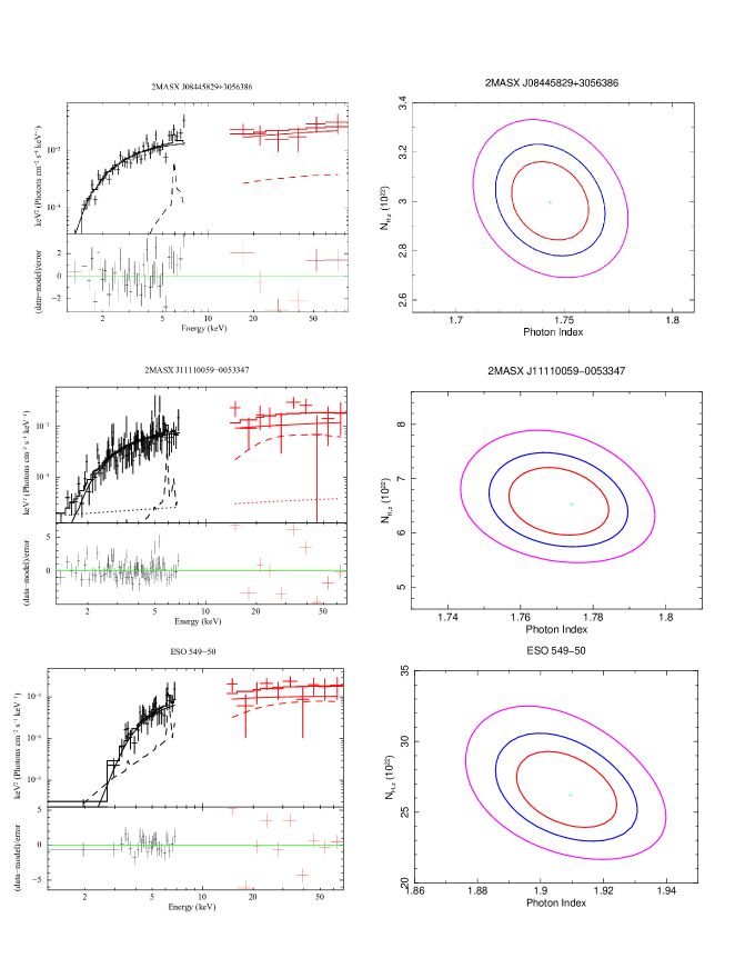
Figure 6: Unfolded Chandra (black) and BAT (red) spectrum of each source fitted with the borus02 model. The best-fitting line-of-sight component is plotted as a solid line, while the reflection component is a dashed line and the scattered component is a dotted line. The confidence contours at 68%, 90%, and 99% are displayed for $\Gamma$ and N_H,Z (in units of 10²² cm^-2).

Table 4: 2MASX J02051994$-$0233055

Model	MYTorus	MYTorus	MYTorus	MYTorus	borus02	pexmon
	(Coupled)	(Decoupled Face-on)	(Decoupled Edge-on)	Face-on + Edge-on
cstat/dof	59/73	59/73	69/73	59/74	57/72	72/74
$\Gamma$	1.78${}^{+0.13}_{-0.10}$	1.73${}^{+0.03}_{-0.13}$	1.76${}^{+0.13}_{-0.14}$	1.76${}^{+0.02}_{-0.03}$	1.65${}^{+0.09}_{-0.22}$	1.83${}^{+0.20}_{-0.19}$
$N_{H,eq}$	10.00${}^{-}_{-3.80}$	…	…	…	…	5.54${}^{+5.76}_{-3.44}$
norm $10^{-2}$	0.64${}^{+0.07}_{-0.06}$	0.18${}^{+0.18}_{-0.02}$	0.13${}^{+0.13}_{-0.07}$	0.18${}^{+0.02}_{-0.01}$	0.27${}^{+1.23}_{-0.16}$	0.09${}^{+0.10}_{-0.05}$
cf,Tor	…	…	…	…	0.87${}^{+0.11}_{-0.46}$	…
cos($\theta_{obs}$)	0.25${}^{+0.08}_{-0.08}$	…	…	…	0.78${}^{+0.21}_{-0.51}$	0.5*
$N_{H,Z}$	…	10.00${}^{-}_{-7.40}$	0.86${}^{+0.40}_{-0.25}$	10.00${}^{-}_{-7.30}$	10.00*	…
$N_{H,S}$	…	10.00${}^{-}_{-5.80}$	5.0${}^{-}_{-4.05}$	10.00${}^{-}_{-5.80}$	10.00${}^{-}_{-6.45}$	…
$f_{s}$ 10-2	1.90${}^{+4.60}_{-1.29}$	6.69${}^{+5.31}_{-3.09}$	9.29${}^{+8.01}_{-4.04}$	6.72${}^{+5.28}_{-3.22}$	4.08${}^{+11.90}_{-2.63}$	13.19${}^{+16.49}_{-7.71}$
Ccha	1*	1*	1*	1*	1*	1*
L$\rm{}_{2-10\,keV}$					2.08${}^{+0.08}_{-0.10}$ $\times$ 1043
L$\rm{}_{15-55\,keV}$					3.00${}^{+0.70}_{-0.59}$ $\times$ 1043

Notes: Same as Table 2.

Table 5: 2MASX J04075215$-$6116126

Model	MYTorus	MYTorus	MYTorus	borus02
	(Coupled)	(Decoupled Face-on)	(Decoupled Edge-on)
cstat/dof	57/32	56/32	57/32	57/31
$\Gamma$	1.61${}^{+0.12}_{-0.12}$	1.60${}^{+0.13}_{-0.10}$	1.60${}^{+0.13}_{-0.11}$	1.56${}^{+0.09}_{-0.14}$
$N_{H,eq}$	0.30${}^{+0.59}_{-0.15}$	…	…	…
norm $10^{-2}$	0.04${}^{+0.03}_{-0.02}$	0.04${}^{+0.03}_{-0.02}$	0.04${}^{+0.03}_{-0.02}$	0.04${}^{+0.02}_{-0.01}$
cf,Tor	…	…	…	0.90${}^{-}_{-0.85}$
cos($\theta_{obs}$)	0.37${}^{+0.12}_{-}$	…	…	0.90${}^{-}_{-}$
$N_{H,Z}$	…	0.20${}^{+0.07}_{-0.06}$	0.20${}^{+0.08}_{-0.06}$	0.21${}^{+0.04}_{-0.08}$
$N_{H,S}$	…	0.39${}^{+0.57}_{-}$	0.20${}^{+0.64}_{-}$	0.19${}^{+2.32}_{-0.15}$
$f_{s}$ 10-2	2.37${}^{+3.10}_{-}$	2.37${}^{+2.90}_{-2.30}$	2.54${}^{+3.10}_{-}$	2.03*
Ccha	1*	1*	1*	1*
L$\rm{}_{2-10\,keV}$				2.09${}^{+0.37}_{-0.35}$ $\times$ 1042
L$\rm{}_{15-55\,keV}$				3.16${}^{+0.31}_{-0.28}$ $\times$ 1042

Notes: Same as Table 2.

Table 6: 2MASX J08445829$+$3056386

Model	MYTorus	MYTorus	MYTorus	borus02
	(Coupled)	(Decoupled Face-on)	(Decoupled Edge-on)
cstat/dof	204/171	203/171	205/171	201/170
$\Gamma$	1.77${}^{+0.05}_{-0.04}$	1.77${}^{+0.07}_{-0.05}$	1.75${}^{+0.06}_{-0.05}$	1.74${}^{+0.07}_{-0.06}$
$N_{H,eq}$	0.43${}^{+0.44}_{-0.30}$	…	…	…
norm $10^{-2}$	0.10${}^{+0.01}_{-0.01}$	0.10${}^{+0.01}_{-0.01}$	0.10${}^{+0.01}_{-0.01}$	0.09${}^{+0.01}_{-0.01}$
cf,Tor	…	…	…	1.00${}^{-}_{-0.65}$
cos($\theta_{obs}$)	0.50${}^{-}_{-0.02}$	…	…	0.05∗
$N_{H,Z}$	…	0.031${}^{+0.003}_{-0.003}$	0.031${}^{+0.003}_{-0.003}$	0.030 ${}^{+0.003}_{-0.003}$
$N_{H,S}$	…	0.50${}^{+0.62}_{-0.35}$	0.30${}^{+0.42}_{-0.23}$	0.24${}^{+0.22}_{-0.15}$
$f_{s}$ 10-2	0.02${}^{+2.18}_{-}$	0.01${}^{+2.29}_{-}$	0.01${}^{+2.34}_{-}$	0*
Ccha	1*	1*	1*	1*
L$\rm{}_{2-10\,keV}$				3.31${}^{+0.16}_{-0.15}$ $\times$ 1043
L$\rm{}_{15-55\,keV}$				3.89${}^{+0.38}_{-0.34}$ $\times$ 1043

Notes: Same as Table 2.

Table 7: 2MASX J11110059$-$0053347

Model	MYTorus	MYTorus	MYTorus	borus02
	(Coupled)	(Decoupled Face-on)	(Decoupled Edge-on)
cstat/dof	98/74	99/74	97/74	98/74
$\Gamma$	1.63${}^{+0.07}_{-0.06}$	1.64${}^{+0.07}_{-0.08}$	1.69${}^{+0.09}_{-0.08}$	1.77${}^{+0.02}_{-0.19}$
$N_{H,eq}$	0.07${}^{+0.25}_{-0.01}$	…	…	…
norm $10^{-2}$	0.05${}^{+0.01}_{-0.01}$	0.06${}^{+0.01}_{-0.02}$	0.06${}^{+0.02}_{-0.01}$	0.06${}^{+0.02}_{-0.01}$
cf,Tor	…	…	…	0.89${}^{-}_{-}$
cos($\theta_{obs}$)	0.0${}^{+0.5}_{-}$	…	…	0.89${}^{-}_{-}$
$N_{H,Z}$	…	0.07${}^{+0.02}_{-0.02}$	0.06${}^{+0.02}_{-0.02}$	0.07${}^{+0.02}_{-0.02}$
$N_{H,S}$	…	0.01${}^{-}_{-}$	0.96${}^{-}_{-}$	31.62${}^{-}_{-}$
$f_{s}$	0.04${}^{+0.04}_{-}$	0.04${}^{+0.04}_{-}$	0.03${}^{+0.04}_{-}$	0.03${}^{+0.04}_{-0.03}$
Ccha	1*	1*	1*	1*
L$\rm{}_{2-10\,keV}$				3.98${}^{+0.38}_{-0.35}$ $\times$ 1043
L$\rm{}_{15-55\,keV}$				5.01${}^{+0.48}_{-0.44}$ $\times$ 1043

Notes: Same as Table 2.
cstat/dof: Chandra data only.

Table 8: ESO 549$-$50

Model	MYTorus	MYTorus	MYTorus	borus02
	(Coupled)	(Decoupled Face-on)	(Decoupled Edge-on)
cstat/dof	22/13	21/13	22/23	21/23
$\Gamma$	1.81${}^{+0.25}_{-0.14}$	1.86${}^{+0.23}_{-0.15}$	1.81${}^{+0.18}_{-0.10}$	1.91${}^{+0.02}_{-0.02}$
$N_{H,eq}$	0.27${}^{-}_{-0.05}$	…	…	…
norm $10^{-2}$	0.10${}^{+0.09}_{-0.04}$	0.10${}^{+0.10}_{-0.04}$	0.10${}^{+0.09}_{-0.03}$	0.10${}^{+0.10}_{-0.02}$
cf,Tor	…	…	…	0.35${}^{+0.05}_{-0.05}$
cos($\theta_{obs}$)	0.01${}^{+0.49}_{-}$	…	…	0.95${}^{-}_{-0.77}$
$N_{H,Z}$	…	0.25${}^{+0.07}_{-0.04}$	0.26${}^{+0.14}_{-0.06}$	0.26${}^{+0.08}_{-0.06}$
$N_{H,S}$	…	1.6${}^{-}_{-1.59}$	0.50${}^{-}_{-}$	14.13${}^{-}_{-}$
$f_{s}$	0.002${}^{+0.004}_{-}$	0.001*	0.002*	0
Ccha	1*	1*	1*	1*
L$\rm{}_{2-10\,keV}$				3.98${}^{+0.70}_{-0.59}$ $\times$ 1042
L$\rm{}_{15-55\,keV}$				3.72${}^{+0.36}_{-0.33}$ $\times$ 1042

Notes: Same as Table 7.

Table 9: IRAS 11058$-$1131

Model	MYTorus	MYTorus	MYTorus	borus02
	(Coupled)	(Decoupled Face-on)	(Decoupled Edge-on)
cstat/dof	11/6	11/6	11/6	11/6
$\Gamma$	1.41${}^{+0.61}_{-}$	1.45${}^{+0.25}_{-}$	1.41${}^{+0.40}_{-}$	1.45${}^{+0.35}_{-}$
$N_{H,eq}$	10.00${}^{-}_{-}$	…	…	…
norm $10^{-2}$	0.20${}^{+3.30}_{-0.20}$	0.04${}^{+0.04}_{-0.03}$	0.04${}^{+0.12}_{-0.02}$	0.04${}^{+0.16}_{-0.02}$
cf,Tor	…	…	…	0.60${}^{-}_{-}$
cos($\theta_{obs}$)	0.15${}^{+0.35}_{-}$	…	…	0.05*
$N_{H,Z}$	…	2.60${}^{-}_{-1.93}$	0.94${}^{-}_{-0.93}$	0.81${}^{+0.84}_{-0.74}$
$N_{H,S}$	…	9.04${}^{-}_{-6.88}$	8.75${}^{-}_{-}$	7.41${}^{-}_{-}$
$f_{s}$	0.003${}^{+0.099}_{-0.003}$	0.02${}^{+0.03}_{-0.01}$	0.02${}^{-}_{-0.02}$	0.03${}^{-}_{-}$
Ccha	1.13${}^{+5.27}_{-1.02}$	0.88${}^{+0.91}_{-0.87}$	0.92${}^{-}_{-0.91}$	0.70${}^{+5.30}_{-0.69}$
L$\rm{}_{2-10\,keV}$				1.55${}^{+1.47}_{-1.06}$ $\times$ 1043
L$\rm{}_{15-55\,keV}$				3.16${}^{+0.31}_{-0.28}$ $\times$ 1043

Notes: Same as Table 7.
BAT cross-norm fixed at 1.

Table 10: MCG $+$08-33-046

Model	pileup
cstat/dof	86/77
$\Gamma$	2.05
$N_{H,eq}$	0.02
norm $10^{-2}$	0.32
cf,Tor	…
cos($\theta_{obs}$)	…
$N_{H,Z}$	…
$N_{H,S}$	…
$f_{s}$	…
Ccha	1*
L$\rm{}_{2-10\,keV}$	4.90${}^{+0.47}_{-0.43}$ $\times$ 1042
L$\rm{}_{15-55\,keV}$	3.55${}^{+0.17}_{-0.16}$ $\times$ 1042

Notes: Same as Table 7.

Table 11: IRAS 12571$+$7643

Model	MYTorus	MYTorus	MYTorus	borus02
	(Coupled)	(Decoupled Face-on)	(Decoupled Edge-on)
cstat/dof	44/30	44/30	43/30	41/30
$\Gamma$	1.69${}^{+0.11}_{-0.11}$	1.71${}^{+0.12}_{-0.10}$	1.75${}^{+0.13}_{-0.14}$	1.61${}^{+0.18}_{-0.07}$
$N_{H,eq}$	0.17${}^{+0.45}_{-0.03}$	…	…	…
norm $10^{-2}$	0.07${}^{+0.02}_{-0.01}$	0.08${}^{+0.01}_{-0.01}$	0.07${}^{+0.03}_{-0.02}$	0.05${}^{+0.02}_{-0.01}$
cf,Tor	…	…	…	0.15${}^{-}_{-}$
cos($\theta_{obs}$)	0.0${}^{+0.5}_{-}$	…	…	0.90${}^{-}_{-}$
$N_{H,Z}$	…	0.18${}^{+0.06}_{-0.03}$	0.17${}^{+0.05}_{-0.05}$	0.16${}^{+0.05}_{-0.03}$
$N_{H,S}$	…	0.02${}^{+0.44}_{-}$	0.90${}^{-}_{-}$	0.01${}^{-}_{-}$
$f_{s}$	0.01${}^{+0.01}_{-0.01}$	0.01${}^{+0.01}_{-0.01}$	0.01${}^{+0.02}_{-0.01}$	0.01${}^{+0.01}_{-}$
Ccha	1*	1*	1*	1*
L$\rm{}_{2-10\,keV}$				2.09${}^{+0.25}_{-0.27}$ $\times$ 1043
L$\rm{}_{15-55\,keV}$				3.63${}^{+0.17}_{-0.16}$ $\times$ 1043

Notes: Same as Table 7.

Appendix B Chandra Exposures

Table 12: BAT 95% Confidence Regions

Swift-BAT ID	Source Name	95% Region
		Arcmin
J0205.2$-$0232	2MASX J02051994$-$0233055∗	2.76
J0402.6$-$2107	ESO 549$-$50†	4.49
J0407.8$-$6116	2MASX J04075215$-$6116126∗	3.40
J0844.8$+$3055	2MASX J08445829$+$3056386∗	2.95
J0901.8$-$6418	ESO 090$-$IG 014∗	2.87
J1108.4$-$1148	IRAS 11058$-$1131†	4.73
J1111.0$+$0054	2MASX J11110059$-$0053347†	4.65
J1258.4$+$7624	IRAS 12571+7643†	4.35
J1828.8$+$5021	MCG $+$08-33-046†	3.77

Notes:
$*$: From the 100-month BAT Catalog.
$\dagger$: From the 150-month BAT Catalog.

References

- Aird et al. (2015) Aird, J., Alexander, D. M., Ballantyne, D. R., et al. 2015, The Astrophysical Journal, 815, 66
- Ajello et al. (2008) Ajello, M., Greiner, J., Sato, G., et al. 2008, The Astrophysical Journal, 689, 666
- Ajello et al. (2008) Ajello, M., Rau, A., Greiner, J., et al. 2008, ApJ, 673, 96
- Alexander et al. (2003) Alexander, D. M., Bauer, F. E., Brandt, W. N., et al. 2003, The Astronomical Journal, 126, 539
- Ananna et al. (2019) Ananna, T. T., Treister, E., Urry, C. M., et al. 2019, ApJ, 871, 240
- Annuar et al. (2020) Annuar, A., Alexander, D. M., Gandhi, P., et al. 2020, MNRAS, 497, 229
- Arnaud (1996) Arnaud, K. A. 1996, in Astronomical Society of the Pacific Conference Series, Vol. 101, Astronomical Data Analysis Software and Systems V, ed. G. H. Jacoby & J. Barnes, 17
- Arp & Madore (1987) Arp, H. C., & Madore, B. 1987, A catalogue of southern peculiar galaxies and associations
- Asmus et al. (2015) Asmus, D., Gandhi, P., Hönig, S. F., Smette, A., & Duschl, W. J. 2015, MNRAS, 454, 766
- Asmus et al. (2020) Asmus, D., Greenwell, C. L., Gandhi, P., et al. 2020, MNRAS, 494, 1784
- Baloković et al. (2018) Baloković, M., Brightman, M., Harrison, F. A., et al. 2018, ApJ, 854, 42
- Barthelmy et al. (2005) Barthelmy, S. D., Barbier, L. M., Cummings, J. R., et al. 2005, Space Science Reviews, 120, 143–164
- Bianchi et al. (2012) Bianchi, S., Panessa, F., Barcons, X., et al. 2012, MNRAS, 426, 3225
- Brightman & Nandra (2011) Brightman, M., & Nandra, K. 2011, MNRAS, 413, 1206
- Buchner et al. (2019) Buchner, J., Brightman, M., Nandra, K., Nikutta, R., & Bauer, F. E. 2019, A&A, 629, A16
- Burlon et al. (2011) Burlon, D., Ajello, M., Greiner, J., et al. 2011, The Astrophysical Journal, 728, 58
- Civano et al. (2015) Civano, F., Hickox, R. C., Puccetti, S., et al. 2015, The Astrophysical Journal, 808, 185
- Comastri (2004) Comastri, A. 2004, Astrophysics and Space Science Library, Vol. 308, Compton-Thick AGN: The Dark Side of the X-Ray Background, ed. A. J. Barger, 245
- Cusumano et al. (2014) Cusumano, G., Segreto, A., La Parola, V., & Maselli, A. 2014, in Proceedings of Swift: 10 Years of Discovery (SWIFT 10, 132
- Cusumano et al. (2010) Cusumano, G., La Parola, V., Segreto, A., et al. 2010, A&A, 524, A64
- Davis (2001) Davis, J. E. 2001, ApJ, 562, 575
- Della Ceca et al. (2008) Della Ceca, Caccianiga, A., Severgnini, P., et al. 2008, A&A, 487, 119
- Durré & Mould (2018) Durré, M., & Mould, J. 2018, ApJ, 867, 149
- Fabbiano et al. (2017) Fabbiano, G., Elvis, M., Paggi, A., et al. 2017, ApJ, 842, L4
- Fabbiano et al. (2018) Fabbiano, G., Paggi, A., Karovska, M., et al. 2018, ApJ, 865, 83
- Fruscione et al. (2006) Fruscione, A., McDowell, J. C., Allen, G. E., et al. 2006, in Observatory Operations: Strategies, Processes, and Systems, ed. D. R. Silva & R. E. Doxsey, Vol. 6270, International Society for Optics and Photonics (SPIE), 586 – 597
- Gandhi & Fabian (2003) Gandhi, P., & Fabian, A. C. 2003, MNRAS, 339, 1095
- Gehrels et al. (2004) Gehrels, N., Chincarini, G., Giommi, P., et al. 2004, The Astrophysical Journal, 611, 1005
- George & Fabian (1991) George, I. M., & Fabian, A. C. 1991, MNRAS, 249, 352
- Gilli et al. (2007) Gilli, Comastri, A., & Hasinger, G. 2007, A&A, 463, 79
- Guo et al. (2021) Guo, X., Gu, Q., Ding, N., Yu, X., & Chen, Y. 2021, ApJ, 908, 169
- Harrison et al. (2016) Harrison, F. A., Aird, J., Civano, F., et al. 2016, The Astrophysical Journal, 831, 185
- Hickox & Markevitch (2006) Hickox, R. C., & Markevitch, M. 2006, The Astrophysical Journal, 645, 95
- Jones et al. (2020) Jones, M. L., Fabbiano, G., Elvis, M., et al. 2020, ApJ, 891, 133
- Jones et al. (2021) Jones, M. L., Parker, K., Fabbiano, G., et al. 2021, ApJ, 910, 19
- Kalberla et al. (2005) Kalberla, Burton, W. B., Hartmann, Dap, et al. 2005, A&A, 440, 775
- Kilerci Eser et al. (2020) Kilerci Eser, E., Goto, T., Güver, T., Tuncer, A., & Ataş, O. H. 2020, MNRAS, 494, 5793
- Koss et al. (2017) Koss, M., Trakhtenbrot, B., Ricci, C., et al. 2017, ApJ, 850, 74
- Koss et al. (2016) Koss, M. J., Assef, R., Baloković, M., et al. 2016, ApJ, 825, 85
- Lanzuisi et al. (2013) Lanzuisi, G., Civano, F., Elvis, M., et al. 2013, Monthly Notices of the Royal Astronomical Society, 431, 978
- Lanzuisi et al. (2018) Lanzuisi, G., Civano, F., Marchesi, S., et al. 2018, MNRAS, 480, 2578
- Liu & Li (2014) Liu, Y., & Li, X. 2014, ApJ, 787, 52
- Ma et al. (2020) Ma, J., Elvis, M., Fabbiano, G., et al. 2020, ApJ, 900, 164
- Magdziarz & Zdziarski (1995) Magdziarz, P., & Zdziarski, A. A. 1995, MNRAS, 273, 837
- Marchesi et al. (2017a) Marchesi, S., Ajello, M., Comastri, A., et al. 2017a, ApJ, 836, 116
- Marchesi et al. (2019) Marchesi, S., Ajello, M., Zhao, X., et al. 2019, ApJ, 882, 162
- Marchesi et al. (2017b) Marchesi, S., Tremblay, L., Ajello, M., et al. 2017b, The Astrophysical Journal, 848, 53
- Mullaney et al. (2015) Mullaney, J. R., Del-Moro, A., Aird, J., et al. 2015, The Astrophysical Journal, 808, 184
- Murphy & Yaqoob (2009) Murphy, K. D., & Yaqoob, T. 2009, MNRAS, 397, 1549
- Nandra et al. (2007) Nandra, K., O’Neill, P. M., George, I. M., & Reeves, J. N. 2007, MNRAS, 382, 194
- Oh et al. (2018) Oh, K., Koss, M., Markwardt, C. B., et al. 2018, ApJS, 235, 4
- Paturel et al. (2003) Paturel, G., Petit, C., Prugniel, P., et al. 2003, A&A, 412, 45
- Ricci et al. (2015) Ricci, C., Ueda, Y., Koss, M. J., et al. 2015, The Astrophysical Journal, 815, L13
- Ricci et al. (2017) Ricci, C., Trakhtenbrot, B., Koss, M. J., et al. 2017, ApJS, 233, 17
- Risaliti et al. (2002) Risaliti, G., Elvis, M., & Nicastro, F. 2002, ApJ, 571, 234
- Risaliti et al. (1999) Risaliti, G., Maiolino, R., & Salvati, M. 1999, The Astrophysical Journal, 522, 157
- Segreto et al. (2010) Segreto, A., Cusumano, G., Ferrigno, C., et al. 2010, A&A, 510, A47
- Tanimoto et al. (2019) Tanimoto, A., Ueda, Y., Odaka, H., et al. 2019, ApJ, 877, 95
- Torres-Albà et al. (2021) Torres-Albà, N., Marchesi, S., Zhao, X., et al. 2021, ApJ, 922, 252
- Torricelli-Ciamponi et al. (2014) Torricelli-Ciamponi, G., Pietrini, P., Risaliti, G., & Salvati, M. 2014, MNRAS, 442, 2116
- Traina et al. (2021) Traina, A., Marchesi, S., Vignali, C., et al. 2021, ApJ, 922, 159
- Treister et al. (2009) Treister, E., Urry, C. M., & Virani, S. 2009, The Astrophysical Journal, 696, 110
- Ueda et al. (2014) Ueda, Y., Akiyama, M., Hasinger, G., Miyaji, T., & Watson, M. G. 2014, The Astrophysical Journal, 786, 104
- Vasudevan et al. (2013) Vasudevan, R. V., Brandt, W. N., Mushotzky, R. F., et al. 2013, The Astrophysical Journal, 763, 111
- Véron-Cetty & Véron (2006) Véron-Cetty, M. P., & Véron, P. 2006, A&A, 455, 773
- Voges et al. (1999) Voges, W., Aschenbach, B., Boller, T., et al. 1999, A&A, 349, 389
- Worsley et al. (2005) Worsley, M. A., Fabian, A. C., Bauer, F. E., et al. 2005, Monthly Notices of the Royal Astronomical Society, 357, 1281
- Yan et al. (2019) Yan, W., Hickox, R. C., Hainline, K. N., et al. 2019, ApJ, 870, 33
- Yaqoob (2012) Yaqoob, T. 2012, MNRAS, 423, 3360
- Zhao et al. (2019a) Zhao, X., Marchesi, S., & Ajello, M. 2019a, ApJ, 871, 182
- Zhao et al. (2020) Zhao, X., Marchesi, S., Ajello, M., Baloković, M., & Fischer, T. 2020, ApJ, 894, 71
- Zhao et al. (2019b) Zhao, X., Marchesi, S., Ajello, M., et al. 2019b, ApJ, 870, 60