Non-Hermitian squeezed polarons

Abstract

Recent experimental breakthroughs in non-Hermitian ultracold atomic lattices have dangled tantalizing prospects in realizing exotic, hitherto unreported, many-body non-Hermitian quantum phenomena. In this work, we discover and propose an experimental platform for a radically different non-Hermitian phenomenon dubbed polaron squeezing. It is marked by a dipole-like accumulation of fermions arising from an interacting impurity in a background of non-Hermitian reciprocity-breaking hoppings. We computed their spatial density and found that, unlike Hermitian polarons which are symmetrically localized around impurities, non-Hermitian squeezed polarons localize asymmetrically in the direction opposite to conventional non-Hermitian pumping and non-perturbatively modify the entire spectrum, despite having a manifestly local profile. We investigated their time evolution and found that, saliently, they appear almost universally in the long-time steady state, unlike Hermitian polarons which only exist in the ground state. In our numerics, we also found that, unlike well-known topological or skin localized states, squeezed polarons exist in the bulk, independently of boundary conditions. Our findings could inspire the realization of many-body states in ultracold atomic setups, where a squeezed polaron can be readily detected and characterized by imaging the spatial fermionic density.

Introduction.– Rapid recent experimental progress in metamaterial feng2011nonreciprocal ; shen2016experimental ; park2020observation ; coulais2017static ; zhu2018simultaneous ; ghatak2020observation ; brandenbourger2019non ; gao2021non , circuit helbig2020generalized ; hofmann2019chiral ; liu2020gain ; hofmann2020reciprocal ; liu2021non ; zou2021observation ; stegmaier2021topological ; ce2022experimental , photonic xiao2020non ; feng2017non ; tzuang2014non ; zhou2018observation ; zhen2015spawning ; zeuner2015observation ; xiao2020non ; miri2019exceptional , and ultracold atomic Jiaming2019gainloss ; lapp2019engineering ; ren2022chiral ; liang2022dynamic ; yi2022exceptional ; gou2020tunable realizations of non-Hermitian models have made unconventional features such as exceptional branch points Bergholtz2021rmp ; lafalce2019robust ; kozii2017non ; yoshida2019exceptional ; yoshida2019symmetry ; okugawa2019topological ; hodaei2017enhanced ; heiss2016circling ; heiss2012physics and non-Hermitian topological windings gong2018topological ; yoshida2018non ; zhang2020correspondence ; zhong2018winding ; rafi2021topological ; yoshida2019mirror ; sun2020biorthogonal ; xi2021classification experimental realities. However, to date, their explorations have mostly been confined to the single-body paradigm, with associated phenomena such as gapped topological transitions lee2020unraveling ; li2021non , unconventional criticality li2020critical , negative entanglement entropy chang2020entanglement ; lee2020exceptional ; okuma2021quantum , and the breakdown of bulk-boundary correspondences yao2018edge ; xiong2018does ; lee2019anatomy ; Kunst2018prl ; Yokomizo2019prl ; Imura2019prb ; Song2019BBC ; borgnia2020non ; li2021quantized ; lv2021curving ; yang2022designing ; jiang2022dimensional ; tai2022zoology . But even more intriguing, many-body phenomena have come within the horizon ever since the very recent experimental breakthroughs in non-Hermitian ultracold atomic setups Jiaming2019gainloss ; lapp2019engineering ; ren2022chiral ; liang2022dynamic ; yi2022exceptional ; gou2020tunable . The interplay of non-Hermiticity with many-body effects has now become a possibility, as captured by emerging directions such as non-Hermitian many-body localization Hamazaki2019prl ; Zhai2020prb ; suthar2022non ; wang2022non , superfluids luo2020skin ; Zhang2020prb ; Liu2020prb ; zhou2019enhanced ; Zhou2020pra ; pan2021emergent , and Fermi liquids lee2021many ; Shen2021arxiv ; Pan2020np ; kawabata2022many ; yamamoto2019theory ; alsallom2021fate ; zhang2022symmetry ; poddubny2022topologically ; yoshida2022fate .

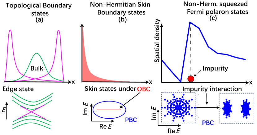
Figure 1: Non-Hermitian polaron squeezing is distinct from other mechanisms for localized states, such as (a) topological localization and (b) the non-Hermitian skin effect, both single-body mechanisms requiring open boundaries. By contrast, squeezed polarons (c) are special asymmetric dipole-like accumulations across either side of an interacting impurity. They are many-body dressed states in the bulk, with charge density “squeezed” in the opposite direction from non-Hermitian pumping. Illustrative numerics are from $\hat{H}_{\text{min}}$ of Eq. (1).

In this work, through exact diagonalization computations Weinberg2017QuSpin ; Weinberg2019QuSpin , we discover a non-Hermitian many-body phenomenon dubbed “polaron squeezing”, which is a directional dipole-like accumulation effect arising from the triple interplay of impurity interactions, fermionic statistics, and non-Hermitian flux. In conventional Hermitian settings, polarons are many-body states dressed by the environment-impurity interaction, as observed in ultracold-atom experiments involving both fermions Schirotzek2009prl ; Zhang2021prl ; Kohstall2012nature ; Koschorreck2012nature ; Cetina2016science ; Scazza2017prl ; Yan2019prl ; oppong2019observation ; Ness2020prx and bosons Hu2016prl ; Jorgensen2016prl ; Yan2020science . By providing a unique angle for understanding strong interactions in solid-state and cold-atom systems, they are valuable probes for detecting quantum phase transitions in interacting topological settings hu2013universal ; lee2014lattice ; lee2015geometric ; grusdt2016interferometric ; Camacho2019prb ; Pimenov2021prb ; qin2019polaron .

Going beyond well-understood Hermitian polarons Chevy2006pra ; Lobo2006prl ; Combescot2007prl ; Bruun2010prl ; Mathy2011prl ; zollner2011polarons ; parish2011polaron ; levinsen2012p ; Yi2012prl ; Parish2013pra ; Yi2015pra ; nishida2015polaronic ; parish2016quantum ; Camacho2018prl ; qin2019polaron ; cui2020fermi ; pessoa2021finite ; ardila2021dynamical ; seetharam2021dynamical ; seetharam2021quantum ; hu2022crossover ; qin2022light ; qin2022phase ; qin2020theory , we found that, with non-Hermiticity and flux, polarons can acquire interesting aggregate behavior, with chiral delocalizing tendencies competing with impurity localization, in a way distinct from non-interacting impurities under the non-Hermitian skin effect (NHSE) li2021impurity . Fermion degeneracy pressure introduces another level of intrigue by enforcing a special type of equilibrium among these competing influences. The result is a unique real-space “squeezed” fermionic density profile that, as we show, can be feasibly imaged in a realistic ultracold atomic demonstration.

Arising from predominantly many-body mechanisms, squeezed polaron states are distinct from other existing well-known types of robust states in related physical settings. Chiral topological states Hasan2010rmp ; Chiu2016rmp [Fig. 1(a)], for instance, are edge localized and asymmetrically propagating, but they originate from nontrivial Chern topology, which is already completely well-defined in the single-particle context. Non-Hermitian boundary-localized skin states yao2018edge ; xiong2018does ; lee2019anatomy ; Kunst2018prl ; Yokomizo2019prl ; Imura2019prb ; Song2019BBC [Fig. 1(b)] are also essentially single-particle phenomena, with their robustness stemming from the directed non-Hermitian “pumping” in non-reciprocal lattices. In contrast, squeezed polarons [Fig. 1(c)] are bona fide many-body states localized beside an impurity interacting with the fermions, and they can exist without nontrivial topology or physical boundaries. Due to their many-body nature, squeezed polarons also exhibit spatial profiles that are very different from those of topological or skin states.

Squeezed polarons from interactions and non-reciprocal gain and loss.– To understand the primary mechanism behind polaron squeezing, we first examine a minimal toy model $\hat{H}_{\text{min}}$ where fermions interact with a single impurity with strength $g$ and hop asymmetrically with amplitudes $e^{\pm\alpha}$ around a ring with circumference $L$ that gives periodic boundary conditions (PBCs):

$$\hat{H}_{\text{min}}\!=\!g\hat{b}^{\dagger}_{x_{0}}\hat{b}_{x_{0}}\hat{c}^{\dagger}_{x_{0}}\hat{c}_{x_{0}}\!+\!\sum_{x}(e^{\alpha}\hat{c}_{x}^{\dagger}\hat{c}_{x+1}\!+\!e^{-\alpha}\hat{c}_{x+1}^{\dagger}\hat{c}_{x}).$$ (1)

Here $\hat{c}$ and $\hat{b}$ are respectively the second-quantized operators for the fermions and the impurity, which is fixed at an arbitrary site $x_{0}$. They experience a density-density interaction of strength $g$. The fermions also experience asymmetric hoppings $e^{\pm\alpha}$, which are the simplest possible terms that represent the simultaneous breaking of Hermiticity and reciprocity . Importantly, due to the PBCs, these asymmetric hoppings cannot be “gauged away” as in conventional literature on the boundary accumulation of non-Hermitian skin states yao2018edge ; lee2019anatomy . This independence from boundary accumulation is the first hint of the fundamental distinction between squeezed polarons and topological as well as skin states.

Squeezed polarons arise when the two parameters $g$ and $\alpha$ of $\hat{H}_{\text{min}}$ are both nonzero and sufficiently large. To elucidate their behavior, we turn on $g$ and $\alpha$ under PBCs and observe how that affects the energy spectrum and long-time steady-state spatial density

$$\rho(x)\equiv\lim_{t\to\infty}\langle\psi^{R}(t)|\hat{c}_{x}^{\dagger}\hat{c}_{x}|\psi^{R}(t)\rangle.$$ (2)

Here $|\psi^{R}(t)\rangle=e^{-i\hat{H}t}\left|\psi^{R}(0)\right\rangle/\left\|e^{-i\hat{H}t}\left|\psi^{R}(0)\right\rangle\right\|$ is the normalized $N$-fermion right eigenstate that has time evolved from a specified initial state $\left|\psi^{R}(0)\right\rangle$. This evolution is taken over a sufficiently long time $t$, such that the spatial density approaches a steady spatial configuration.

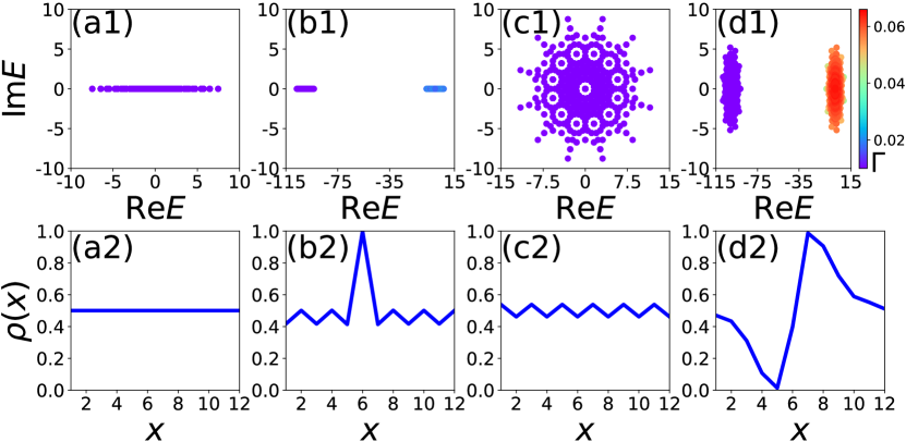
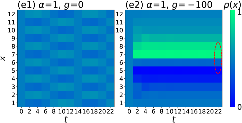
Figure 2: PBC spectrum $E$ [panels (a1)-(d1)] and spatial density $\rho(x)$ [panels (a2)-(d2)] for $\hat{H}_{\text{min}}$ [Eq. (1)] with different non-reciprocities $\alpha$ and impurity interaction strengths $g$: (a1,a2) $\alpha=g=0$; (b1,b2) $\alpha=0$, $g=-100$; (c1,c2) $\alpha=1$, $g=0$; and (d1,d2) $\alpha=1$, $g=-100$. Energy eigenstates $|\psi\rangle$ are colored by their squeezing asymmetric parameter $\Gamma$, which captures polaron squeezing: $\Gamma$ is large only with both non-reciprocity and impurity interaction (d1). While the spatial polaron density $\rho(x)$ is symmetrically peaked about the impurity at $x_{0}=6$ when Hermitian (b2), it is asymmetrically squeezed in the non-Hermitian case (d2). (e1,e2) Dynamics of the spatial density for (e1) $\alpha=1$, $g=0$ and for (e2) $\alpha=1$, $g=-100$, with the dipole-like asymmetric profile as circled. All computations are with $N=6$ fermions in $L=12$ sites. The initial state $\left|\psi^{R}(0)\right\rangle$ is the ground state for $\alpha=0$ and is $(\left|101010101010\right\rangle+\left|010101010101\right\rangle)/\sqrt{2}$ for $\alpha=1$ supp .

When $\alpha=g=0$ [Figs. 2(a1) and 2(a2)], we trivially have Hermitian nearest-neighbor hoppings with a real gapless spectrum. Due to translation invariance from PBCs, $\rho(x)=0.5$ everywhere. Turning on the impurity interaction such that $\alpha=0$ and $g=-100$ [Figs. 2(b1) and 2(b2)], we realize a minimal Hermitian polaron bound state, with $\rho(x)$ peaking at the impurity $x_{0}$. It is the polaron bound by the gap which opens up. When we turn on the non-Hermiticity and non-reciprocity instead of the interaction, such that $\alpha=1$ and $g=0$ [Figs. 2(c1) and 2(c2)], $\rho(x)$ is oscillating around $0.5$, and the spectrum becomes complex with $L$ star-like spikes supp . Note that it is not a superposition of the energies of $N$ Hatano-Nelson chains hatano1996localization ; hatano1997vortex ; hatano1998non-Hermitian , since Pauli exclusion constrains certain asymmetric hoppings.

Finally, turning on both the interaction and non-Hermiticity such that $\alpha=1$ and $g=-100$ [Figs. 2(d1) and 2(d2)], we observe a peculiar state with an asymmetric profile $\rho(x)$ around the impurity at $x_{0}+1$, which we name a “squeezed polaron”. The density to the left of $x_{0}+1=7$ (sites 5 and 6) appears to be “squeezed” towards the right (sites 8 and 9) by the impurity interaction, even though, naively, we would have expected the asymmetric $e^{\pm\alpha}\hat{c}_{x}\hat{c}_{x\pm 1}$ couplings to pump the states from right to left instead. Notably, the $\rho(x)$ peak is not exponentially high like topological or non-Hermitian skin states, but instead resembles a finite local dipole within the Fermi sea. The spectrum is complex, and a gap separates two almost identical star-like “bands”, the one with negative $\text{Re}(E)$ containing states bounded by the attractive ($g<0$) impurity interaction.

Interestingly, even though the impurity interaction acts locally, its presence affects the entire spectrum [Fig. 2(d1)], not just states localized around the impurity. This is most saliently revealed through the squeezing asymmetry parameter $\Gamma$ of a given $N$-fermion state $|\psi\rangle$, which we define as

$$\Gamma\equiv\sum_{x=1}^{L}(x-x_{0}-1)e^{-(x-x_{0}-1)^{2}}|\langle\psi|\hat{n}_{x}|\psi\rangle|^{2}/N.$$ (3)

Containing the derivative of a Gaussian kernel, it measures the extent of asymmetric state localization around the the impurity neighbor $x_{0}+1$, unlike the more commonly used inverse participation ratio (IPR) parameter hikami1986localization , which is agnostic to the localization asymmetry and position. In particular, it distinguishes our squeezed polarons from ordinary polarons in Hermitian settings, which are symmetric about the impurity. As a reference, a profile with a perfectly localized surplus particle on each side has $\Gamma=2/(Ne)\approx 0.74/N$, which is just slightly higher than the $\Gamma$ of the eigenstates with polaron squeezing behavior [Figs. 2(d1) and 3(b2)]. This also implies that the squeezed polaron is distributed across all bound states, and not particular ground states as with ordinary polarons. Physically, this is because the impurity interaction has become effectively non-local in the background of non-reciprocal gain and loss pumping; but contrary to a simple pumping of states, what we observe is an interaction-facilitated “squeezing” in the opposite direction that results in a dipole-like density profile. Herein lies an important physical distinction between Hermitian polarons and non-Hermitian squeezed polarons - while squeezed polaron asymmetry can be observed in the long-time steady state evolved from most generic initial states  [Fig. 2(e2)], Hermitian (symmetric) polaron localization only exists for the ground state (Fig. S8 of supp ).

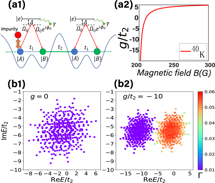
Figure 3: (a1) Our effective interacting Hamiltonian for squeezed polarons [Eq. (5)] is based on a two-photon dissipative Raman process Zhou2020pra ; gou2020tunable with impurity interactions $g$ from Feshbach resonance. The Rabi frequency is $\Omega_{0}$ between hyperfine ground states $|A\rangle$ and $|B\rangle$ and the excited state $|e\rangle$ for ⁴⁰K atoms; a phase difference $\phi_{0}$ introduces non-reciprocity. $\Delta$ is the single-photon detuning of the excited state $|e\rangle$, whose non-Hermitian decay rate $\gamma$ can be laser controlled. (a2) The impurity interaction $g$ is highly tunable through the magnetic field, with parameters given by Refs. Liao2010nature ; Regal2004prl ; Chin2010rmp . (b1,b2) $g$ non-perturbatively modifies the PBC spectrum $E$ at half-filling $N=6$ and $2L=12$, such that all states $|\psi\rangle$ become squeezed with elevated squeezing asymmetry $\Gamma$ when $|g|\neq 0$. Here, $t_{2}=(2\pi)\times 1000$ Hz Atala2013np sets the energy scale.

Ultracold atomic model for observing squeezed polarons.– Having discussed the essential though simplified mechanism behind squeezed polarons, we now turn to a more realistic setup without asymmetric physical couplings and that can be feasibly implemented in an ultracold atomic setup.

The key ingredients for squeezed polarons are (i) impurity interaction, (ii) non-reciprocity, and (iii) loss. To incorporate them all, we consider a one-dimensional fermionic array of $N$ fermionic ⁴⁰K atoms, with the majority being spin $\uparrow$ and the minority being spin $\downarrow$ impurities.

To implement the impurity interaction (i), we apply an external magnetic field $B$ that causes the atoms to experience a strong Feshbach resonance Olshanii1998prl ; Olshanii2003prl ; Chin2010rmp ; Qin20201pra ; Qin20202pra ; Chin2010rmp ; Regal2004prl ; Regal2003prl ; Qin2016pra ; Qin2017epjd that corresponds to a density-density $S$-wave interaction,

$$\hat{H}_{\text{int}}=g\hat{n}_{x_{0},s}^{(b)}\hat{n}_{x_{0},s},$$ (4)

between unlike (majority and impurity) spins, where $\hat{n}_{x_{0},s}^{(b)}=\hat{b}_{x_{0},s}^{\dagger}\hat{b}_{x_{0},s}$ is the number density operator of the spin-$\downarrow$ impurity atom, which is situated at site $s$ of the $x_{0}$th unit cell, and $\hat{n}_{x_{0},s}=\hat{c}_{x_{0},s}^{\dagger}\hat{c}_{x_{0},s}$ is the corresponding density operator of spin-$\uparrow$ majority atoms at the same position. The interaction strength $g\sim g_{0}(B-B_{c})^{-1}$ becomes very strong and saturates at a large value near a resonant magnetic field  $B=B_{c}$, as numerically computed Olshanii1998prl ; Olshanii2003prl ; Chin2010rmp ; Qin20201pra ; Qin20202pra and plotted in Fig. 3(a2), and can be tuned to any desired strength between $-1000t_{2}$ and $\approx 1500t_{2}$ by appropriately adjusting the field strength supp .

A non-reciprocal lattice with loss [(ii) and (iii)] can be achieved by coupling a two-photon dissipative Raman process to the discrete hyperfine ground states $|A\rangle$ and $|B\rangle$ liang2022dynamic ; Zhou2020pra ; gou2020tunable ; Lin2009prl ; Lin2011nature ; Zhang2012prl ; Wang2012prl ; Cheuk2012prl ; Qu2013pra ; li2019topology of each degenerate ⁴⁰K atom and subjecting the atoms to a strong periodic optical potential gou2020tunable ; Atala2013np ; Folling2007nature , as schematically illustrated in Fig. 3(a1). Non-reciprocity is introduced through the phase difference $\phi_{0}$ between the optical fields exciting each hyperfine state; for maximum time-reversal breaking, we set $\phi_{0}=\pi/2$. By adiabatically eliminating  the excited state $|e\rangle$, one obtains an effective spin-orbit coupling in the pseudospin basis of $|A\rangle$ and $|B\rangle$. If the excited state additionally experiences laser-induced decay of rate $\gamma$, the coupling becomes effectively complex , leading to an effective tight-binding Hamiltonian ($\hbar=1$),

$$\hat{H} =\sum_{x}^{L}\left[\left(t_{1}+\tilde{\gamma}\right)\hat{c}_{x,A}^{\dagger}\hat{c}_{x,B}+\left(t_{1}-\tilde{\gamma}\right)\hat{c}_{x,B}^{\dagger}\hat{c}_{x,A}\right.$$

$$~{}~{}+\left.t_{2}(\hat{c}_{x+1,A}^{\dagger}\hat{c}_{x,B}+{\rm H.c.})\right]+g\hat{n}_{x_{0},s}^{(b)}\hat{n}_{x_{0},s}-i\tilde{\gamma}\sum_{x,s}^{L}\hat{n}_{x,s},$$ (5)

where $t_{1}$ and $t_{2}$ depend on the optical potential supp and

$$\tilde{\gamma}=\frac{\Omega_{0}^{2}}{\gamma+i\Delta}$$ (6)

is the effective decay rate, where $\Omega_{0}$ and $\Delta$ are the single-photon Rabi frequency and detuning respectively. The effective intra-cell hoppings $t_{1}\pm\tilde{\gamma}$ have become asymmetric and complex due to the combination of the reciprocity breaking and dissipation, even though the physical optical lattice couplings are all symmetric .

Before presenting the numerical results on this model, we briefly outline the experimental specifications for the parameters used. First, a tiny fraction of spin-$\downarrow$ “impurity” atoms can be created by exciting a spin-polarized (spin-$\uparrow$) cloud of ⁴⁰K atoms in the two lowest hyperfine states Schirotzek2009prl ; Koschorreck2012nature via a two-photon Landau-Zener sweep and subsequently cooling it down. The resultant Fermi gas is then loaded onto a one-dimensional optical superlattice potential $V(x)$ Atala2013np ; Folling2007nature , which is formed by superimposing two standing optical lasers with wavelengths $\lambda_{2}=767$ nm (short lattice) and $\lambda_{1}=2\lambda_{2}$ (long lattice) Atala2013np ; Folling2007nature , such that $V(x)=V_{1}\sin^{2}(k_{1}x+\phi_{0}/2)+V_{2}\sin^{2}(k_{2}x+\pi/2)$, where $k_{1}=2\pi/\lambda_{1}$ and $k_{2}=2k_{1}$, corresponding to a unit cell of size $d=767$ nm Atala2013np . By adjusting the laser amplitudes $V_{1}$ and $V_{2}$, the effective lattice couplings $t_{1}$ and $t_{2}$ can be tuned within $(2\pi)\times[60,1000]$ Hz Atala2013np ; supp ; in this work, we set $t_{2}=(2\pi)\times 1000$ Hz Atala2013np as the reference energy unit, and we fix $t_{1}/t_{2}=1$. For the two-photon dissipative Raman process, we used $\Omega_{0}=(2\pi)\times 0.03$ MHz Fu2013pra and $\Delta=(2\pi)\times 1$ MHz for the single photon Rabi frequency and detuning, and we fix the adjustable decay rate from the excited state $|e\rangle$ as $\gamma=(2\pi)\times 6$ MHz Fu2013pra ; Jie2017pra ; Qin2018pra , such that the effective decay rate takes the value $\tilde{\gamma}\sim(0.92-0.15i)t_{2}=(2\pi)\times(0.92-0.15i)$ kHz supp . We fix the impurity at site $s=A$ of the $x_{0}$th cell. In all, lasers are employed for various distinct purposes: defining the optical lattice potential, sweeping to produce the impurities, and Raman transitions and laser-induced dissipation as shown in Fig. 3(a1).

As evident in Figs. 3(b1) and (b2), the effective ultracold-atomic Hamiltonian $\hat{H}$ of Eq. (5) captures the essential polaron behavior already present in the minimal single-component model $\hat{H}_{\text{min}}$ of Eq. (1), with qualitatively similar many-body spectra. At a relatively modest interaction strength of $g=-10t_{2}$, corresponding to $B\approx 203.5$G, the spectrum separates into two distinct “bands”, both of which correspond to squeezed eigenstates. Their squeezed profile $\rho(x)$ (Fig. S6(a1)-S6(d1) supp ) also retains the characteristic asymmetrically squeezed shape, although it also exhibits step-like kinks due to the symmetry breaking from odd (even) $|A\rangle$ ($|B\rangle$) sites supp .

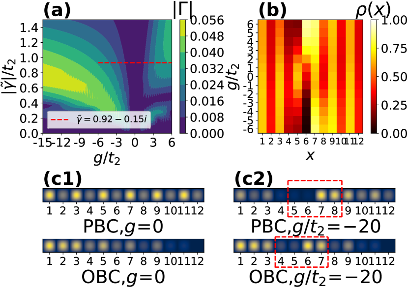
Figure 4: (a) Squeezing expectation $|\Gamma|$ in the $g$-$|\tilde{\gamma}|$ parameter space; note the vanishing squeezing at zero impurity interaction $g$ and the enhanced polaron squeezing at large effective decay rate $|\tilde{\gamma}|$ and very attractive ($g<0$) or repulsive ($g>0$) interactions. Here, $\Gamma$ is computed from the long-time steady state evolved from the initial state $\left|\psi^{R}(0)\right\rangle=(\left|101010101010\right\rangle+\left|010101010101\right\rangle)/\sqrt{2}$. (b) Spatial density $\rho(x)$ as a function of $x$ and $g$ under PBCs. Note the very pronounced asymmetric profile across the impurity position $x_{0}=6$, particularly in the repulsive ($g>0$) case where $\rho(x_{0})$ is strongly localized. Data are plotted at $\tilde{\gamma}/t_{2}=0.92-0.15i$, as indicated by the dashed red line in panel (a). (c1,c2) Simulated spatial density measurements. The density around the impurity ($x_{0}+1=7$) exhibits almost identical asymmetric profiles of squeezed polaron states (red dashed box) regardless of OBCs or PBCs, as long as the impurity interaction $g$ is nonzero, with a slight shift from sublattice effects. (d1,d2) Evolution of spatial densities from the initial state $\left|\psi^{R}(0)\right\rangle$ under PBCs, with an asymmetric steady-state squeezed polaron profile for (d2) $g\neq 0$. We used $\tilde{\gamma}/t_{2}=0.92-0.15i$, $t_{1}/t_{2}=1$, and $N=6$ fermions in $2L=12$ sites for all subfigures, and we used $g=0$ for panels (c1) and (d1) and $g/t_{2}=-20$ for panels (c2) and (d2).

Attractive vs. repulsive polaron squeezing.– Figure 4(a) shows the squeezing expectation $|\Gamma|$  in the parameter space of $g/t_{2}$, the normalized impurity interaction strength, and $|\tilde{\gamma}|/t_{2}$, the normalized effects of reciprocity and dissipation. For Hermitian scenarios with $|\tilde{\gamma}|=0$ and $g\neq 0$, we indeed have vanishing $\Gamma$, as expected from ordinary polarons with symmetric impurity localizations. In general, the squeezing expectation $|\Gamma|$ increases with larger $|\tilde{\gamma}|$ or $|g|$, consistent with the intuition that polaron squeezing requires the combined interplay of interactions, non-reciprocity and non-Hermiticity.

However, Fig. 4(a) also shows a marked asymmetry between attractive ($g<0$) and repulsive ($g>0$) squeezed polarons. A stronger interaction is required to produce an attractive squeezed polaron, relative to a comparably squeezed repulsive polaron. The reason behind this is clear from the plot of spatial density $\rho(x)$ vs $g/t_{2}$ [see Fig. 4(b)], evaluated at the value of $\tilde{\gamma}_{2}=0.92-0.15i$ used in Fig. 3. For attractive polarons with $g<0$, $\rho(x)$ is strongly localized at $x_{0}+1=7$ next to the impurity, leaving a “hole” at the impurity. However, for repulsive polarons with $g>0$, $\rho(x)$ is strongly localized at the impurity position $x_{0}=6$. That said, for both attractive and repulsive cases, the asymmetry in the $\rho(x)$ profile is still strongly contributed by the $\tilde{\gamma}$ asymmetry. In all, repulsive polarons generally possess a stronger combined “dipole” moment and hence larger $\Gamma$.

Independence from boundary conditions.– While we have emphasized that squeezed polarons, unlike skin or topological states, are interacting phenomena and not boundary phenomena, actual experimental lattices are usually bounded . Fortunately, that is not a practical obstacle, because squeezed polarons are largely unaffected by boundary conditions, be they OBCs or PBCs. Shown in Fig. 4(c), there are simulated spatial density of states for $\rho(x)$ measurements with $N=6$ fermions on $2L=12$ sites and the impurity at $x_{0}=6$. Without interactions, i.e., $g=0$ (left), we observe skin boundary accumulation under OBCs but not PBCs. However, squeezed polaron physics dominates in the bulk when the impurity interaction is turned on (right). For both PBCs and OBCs, approximately equal Fermi polaron squeezing (red highlighted) counteracts the background skin accumulation, if any. Despite finite-size effects, polaron squeezing is evidently a robust non-Hermitian interaction effect distinguishable from competing single-body effects away from the boundaries.

Discussion.– With very recent breakthroughs in non-Hermitian cold-atom experiments Jiaming2019gainloss ; lapp2019engineering ; ren2022chiral ; liang2022dynamic ; yi2022exceptional ; gou2020tunable , the physical realization of interacting many-body effects is closer to becoming a practical reality even in non-Hermitian settings. We are hopeful that, through our proposal, squeezed polarons can be measured in the near future, thereby realizing a many-body form of emergent non-locality distinct from non-Hermitian skin sensitivity.

While a squeezed polaron manifests as a local dipole-like density asymmetry, not colossal exponential state localization, it non-perturbatively splits the entire spectrum into two halves, a fascinating demonstration of how particle statistics can help encode non-local effects despite seemingly local density effects. While we have largely demonstrated polaron squeezing with PBCs, it occurs independently of boundaries and remains robust in realistic experimental setups subject to OBCs.

Supplementary Material for “Non-Hermitian Squeezed Polarons”

This appendix contains the following material arranged by sections:

1. Derivation of the effective model.

2. Additional data on the energy spectra and spatial density.

Appendix SI Derivation of the effective model

Here, we rigorously derive the tight-binding model (Eq. (5) of the main text) representing our ultracold atomic setup for non-Hermitian squeezed polarons, beginning with its physical Hamiltonian. Starting from the Schrödinger’s picture formulation for a single unit cell, we switch to the interaction picture to extract the rapidly oscillating phases that can be eliminated via the rotating-wave approximation. Then we go to the rotating frame to eliminate the remaining explicit time dependence. We next treat the most subtle aspect, the dissipative mechanism on the excited state, via the Lindblad master equation, and from it derive the effective non-Hermitian Hamiltonian by adiabatically eliminating the excited state. Incidentally, the latter also agrees with a simple perturbative approach with a phenomenological dissipative term. Next, we consider a 1D array of such setups, and derive a tight-binding Hamiltonian that serves as the non-interacting background of our non-Hermitian squeezed polaron setup.

SI.1 Schrödinger picture

We first ignore any dissipative effects, and derive the effective static Hamiltonian that encapsulates the optical driving. In the Schrödinger picture, our Hamiltonian corresponding to the configuration in Fig. S1 is given by Gou2020prl ; Zhou2020pra

$$\hat{H}_{S}=\frac{\hbar^{2}\hat{k}^{2}}{2m}(|A\rangle\langle A|+|B\rangle\langle B|)+\hbar\omega_{A}|A\rangle\langle A|+\hbar\omega_{B}|B\rangle\langle B|+\hbar\omega_{e}|e\rangle\langle e|+{\bf d}\cdot{\bf E},$$ (S1)

where $|A\rangle$ and $|B\rangle$ are two ground states, $|e\rangle$ is the excited state. The interaction between the atom and light is the dipole interaction ${\bf d}\cdot{\bf E}$ which is given by

$${\bf d}\cdot{\bf E}=(d_{Ae}|A\rangle\langle e|+d_{eA}|e\rangle\langle A|)E_{1}(x,t)+(d_{Be}|B\rangle\langle e|+d_{eB}|e\rangle\langle B|)E_{2}(x,t),$$ (S2)

where $d_{Ae}=-e\langle A|\hat{x}|e\rangle$, $d_{eA}=-e\langle e|\hat{x}|A\rangle$, $d_{Be}=-e\langle B|\hat{x}|e\rangle$, $d_{eB}=-e\langle e|\hat{x}|B\rangle$, and the electric field ${\bf E}={\bf E}_{1}+{\bf E}_{2}$ is given by

$$E_{1}(x,t) = \epsilon_{1}\cos(k_{1}x-\omega_{1}t+\phi_{1})=\frac{\epsilon_{1}}{2}[e^{i(k_{1}x-\omega_{1}t+\phi_{1})}+e^{-i(k_{1}x-\omega_{1}t+\phi_{1})}],$$ (S3)

$$E_{2}(x,t) = \epsilon_{2}\cos(k_{2}x-\omega_{2}t+\phi_{2})=\frac{\epsilon_{2}}{2}[e^{i(k_{2}x-\omega_{2}t+\phi_{2})}+e^{-i(k_{2}x-\omega_{2}t+\phi_{2})}],$$ (S4)

in Fig. S1. Notice that the electric field is classical here.

Substituting Eqs. (S3) and (S4) into (S2), we obtain

$${\bf d}\cdot{\bf E} = \frac{1}{2}\hbar\Omega_{R1}(|A\rangle\langle e|+|e\rangle\langle A|)[e^{i(k_{1}x-\omega_{1}t+\phi_{1})}+e^{-i(k_{1}x-\omega_{1}t+\phi_{1})}]$$ (S5)

$$+ \frac{1}{2}\hbar\Omega_{R2}(|B\rangle\langle e|+|e\rangle\langle B|)[e^{i(k_{2}x-\omega_{2}t+\phi_{2})}+e^{-i(k_{2}x-\omega_{2}t+\phi_{2})}],$$

where the Rabi frequencies are given by the dipole energies

$$\Omega_{R1} = \frac{d_{Ae}\epsilon_{1}}{\hbar}=\frac{d_{eA}\epsilon_{1}}{\hbar},$$ (S6)

$$\Omega_{R2} = \frac{d_{Be}\epsilon_{1}}{\hbar}=\frac{d_{eB}\epsilon_{1}}{\hbar}.$$ (S7)

Figure S1: Schematic of one unit cell of the experimental setup for the dissipative Raman process, without impurity interaction, with quantities in the derivation indicated.

SI.2 Interaction picture

We next perform the Born-Oppenheimer approximation, where we separate the kinetic energy in Eq. (S1), and obtain

$$\hat{H}_{S}=\frac{\hbar^{2}\hat{k}^{2}}{2m}(|A\rangle\langle A|+|B\rangle\langle B|)+\hat{H}_{S0}+{\bf d}\cdot{\bf E},$$ (S8)

where

$$\hat{H}_{S0}=\hbar\omega_{A}|A\rangle\langle A|+\hbar\omega_{B}|B\rangle\langle B|+\hbar\omega_{e}|e\rangle\langle e|.$$ (S9)

Next we go to the interaction picture, where the Hamiltonian is transformed as

$$\hat{H}_{I} =\hat{U}^{\dagger}(t)\hat{H}_{S}\hat{U}(t)-i\hbar\hat{U}^{\dagger}(t)[\partial_{t}\hat{U}(t)]$$ (S10)

$$=\frac{\hbar^{2}\hat{k}^{2}}{2m}(|A\rangle\langle A|+|B\rangle\langle B|)+\exp\left(\frac{i}{\hbar}\hat{H}_{S0}t\right)({\bf d}\cdot{\bf E})\exp\left(-\frac{i}{\hbar}\hat{H}_{S0}t\right)$$

$$=\frac{\hbar^{2}\hat{k}^{2}}{2m}(|A\rangle\langle A|+|B\rangle\langle B|)+\frac{1}{2}\hbar\Omega_{R1}\exp\left(\frac{i}{\hbar}\hat{H}_{S0}t\right)(|A\rangle\langle e|+|e\rangle\langle A|)\exp\left(-\frac{i}{\hbar}\hat{H}_{S0}t\right)[e^{i(k_{1}x-\omega_{1}t+\phi_{1})}+e^{-i(k_{1}x-\omega_{1}t+\phi_{1})}]$$

$$+\frac{1}{2}\hbar\Omega_{R2}\exp\left(\frac{i}{\hbar}\hat{H}_{S0}t\right)(|B\rangle\langle e|+|e\rangle\langle B|)\exp\left(-\frac{i}{\hbar}\hat{H}_{S0}t\right)[e^{i(k_{2}x-\omega_{2}t+\phi_{2})}+e^{-i(k_{2}x-\omega_{2}t+\phi_{2})}]$$

$$=\frac{\hbar^{2}\hat{k}^{2}}{2m}(|A\rangle\langle A|+|B\rangle\langle B|)+\frac{1}{2}\hbar\Omega_{R1}\left[e^{i(\omega_{A}-\omega_{e})t}|A\rangle\langle e|+e^{-i(\omega_{A}-\omega_{e})t}|e\rangle\langle A|\right]\left[e^{i(k_{1}x-\omega_{1}t+\phi_{1})}+e^{-i(k_{1}x-\omega_{1}t+\phi_{1})}\right]$$

$$+\frac{1}{2}\hbar\Omega_{R2}\left[e^{i(\omega_{B}-\omega_{e})t}|B\rangle\langle e|+e^{-i(\omega_{B}-\omega_{e})t}|e\rangle\langle B|\right]\left[e^{i(k_{2}x-\omega_{2}t+\phi_{2})}+e^{-i(k_{2}x-\omega_{2}t+\phi_{2})}\right]$$

$$=\frac{\hbar^{2}\hat{k}^{2}}{2m}(|A\rangle\langle A|+|B\rangle\langle B|)+\frac{1}{2}\hbar\Omega_{R1}\left[e^{-i\omega_{eA}t}|A\rangle\langle e|+e^{i\omega_{eA}t}|e\rangle\langle A|\right]\left[e^{i(k_{1}x-\omega_{1}t+\phi_{1})}+e^{-i(k_{1}x-\omega_{1}t+\phi_{1})}\right]$$

$$+\frac{1}{2}\hbar\Omega_{R2}\left[e^{-i\omega_{eB}t}|B\rangle\langle e|+e^{i\omega_{eB}t}|e\rangle\langle B|\right]\left[e^{i(k_{2}x-\omega_{2}t+\phi_{2})}+e^{-i(k_{2}x-\omega_{2}t+\phi_{2})}\right]$$

$$=\frac{\hbar^{2}\hat{k}^{2}}{2m}(|A\rangle\langle A|+|B\rangle\langle B|)+\frac{1}{2}\hbar\Omega_{R1}\left\{\left[e^{i(k_{1}x-(\omega_{1}+\omega_{eA})t+\phi_{1})}+e^{-i(k_{1}x-(\omega_{1}-\omega_{eA})t+\phi_{1})}\right]|A\rangle\langle e|\right.$$

$$\left.+\left[e^{i(k_{1}x-(\omega_{1}-\omega_{eA})t+\phi_{1})}+e^{-i(k_{1}x-(\omega_{1}+\omega_{eA})t+\phi_{1})}\right]|e\rangle\langle A|\right\}$$

$$+\frac{1}{2}\hbar\Omega_{R2}\left\{\left[e^{i(k_{2}x-(\omega_{2}+\omega_{eB})t+\phi_{2})}+e^{-i(k_{2}x-(\omega_{2}-\omega_{eB})t+\phi_{2})}\right]|B\rangle\langle e|\right.$$

$$\left.+\left[e^{i(k_{2}x-(\omega_{2}-\omega_{eB})t+\phi_{2})}+e^{-i(k_{2}x-(\omega_{2}+\omega_{eB})t+\phi_{2})}\right]|e\rangle\langle B|\right\},$$ (S11)

where we set that $\omega_{eA}=\omega_{e}-\omega_{A}>0$ and $\omega_{eB}=\omega_{e}-\omega_{B}>0$,

$$\hat{U}(t) =\exp\left(-\frac{i}{\hbar}\hat{H}_{S0}t\right),$$ (S12)

$$i\hbar\hat{U}^{\dagger}(t)[\partial_{t}\hat{U}(t)] =i\hbar\exp\left(\frac{i}{\hbar}\hat{H}_{S0}t\right)\left[\partial_{t}\exp\left(-\frac{i}{\hbar}\hat{H}_{S0}t\right)\right]=\hat{H}_{S0}.$$ (S13)

SI.3 Rotating-wave approximation

We next get rid of very rapidly oscillating phases by performing the rotating-wave approximation. Ignoring the counter rotating terms proportional to $e^{\pm i(\omega_{1/2}+\omega_{A/B})t}$, we obtain

$$\hat{H}_{I}^{\rm RWA} =\frac{\hbar^{2}\hat{k}^{2}}{2m}(|A\rangle\langle A|+|B\rangle\langle B|)+\frac{1}{2}\hbar\Omega_{R1}\left[e^{-i(k_{1}x-\Delta_{1A}t+\phi_{1})}|A\rangle\langle e|+e^{i(k_{1}x-\Delta_{1A}t+\phi_{1})}|e\rangle\langle A|\right]$$

$$+\frac{1}{2}\hbar\Omega_{R2}\left[e^{-i(k_{2}x-\Delta_{2B}t+\phi_{2})}|B\rangle\langle e|+e^{i(k_{2}x-\Delta_{2B}t+\phi_{2})}|e\rangle\langle B|\right],$$ (S14)

where $\Delta_{1A}=\omega_{1}-\omega_{eA}$ and $\Delta_{2B}=\omega_{2}-\omega_{eB}$ are both single-photon detunings.

Then, we transfer the above Hamiltonian back to Schrödinger picture:

$$\hat{H}_{S}^{\rm RWA} =\hat{U}(t)\hat{H}_{I}^{\rm RWA}\hat{U}^{\dagger}(t)+i\hbar[\partial_{t}\hat{U}(t)]\hat{U}^{\dagger}(t)$$ (S15)

$$=\hat{U}(t)(\hat{H}_{I}+\hat{H}_{S0})\hat{U}^{\dagger}(t)$$

$$=\frac{\hbar^{2}\hat{k}^{2}}{2m}(|A\rangle\langle A|+|B\rangle\langle B|)+\hbar\omega_{A}|A\rangle\langle A|+\hbar\omega_{B}|B\rangle\langle B|+\hbar\omega_{e}|e\rangle\langle e|$$

$$+\frac{1}{2}\hbar\Omega_{R1}\left[e^{-i(k_{1}x-(\Delta_{1A}+\omega_{eA})t+\phi_{1})}|A\rangle\langle e|+e^{i(k_{1}x-(\Delta_{1A}+\omega_{eA})t+\phi_{1})}|e\rangle\langle A|\right]$$

$$+\frac{1}{2}\hbar\Omega_{R2}\left[e^{-i(k_{2}x-(\Delta_{2B}+\omega_{eB})t+\phi_{2})}|B\rangle\langle e|+e^{i(k_{2}x-(\Delta_{2B}+\omega_{eB})t+\phi_{2})}|e\rangle\langle B|\right]$$

$$=\frac{\hbar^{2}\hat{k}^{2}}{2m}(|A\rangle\langle A|+|B\rangle\langle B|)+\hbar\omega_{A}|A\rangle\langle A|+\hbar\omega_{B}|B\rangle\langle B|+\hbar\omega_{e}|e\rangle\langle e|$$

$$+\frac{1}{2}\hbar\Omega_{R1}\left[e^{-i(k_{1}x-\omega_{1}t+\phi_{1})}|A\rangle\langle e|+e^{i(k_{1}x-\omega_{1}t+\phi_{1})}|e\rangle\langle A|\right]$$

$$+\frac{1}{2}\hbar\Omega_{R2}\left[e^{-i(k_{2}x-\omega_{2}t+\phi_{2})}|B\rangle\langle e|+e^{i(k_{2}x-\omega_{2}t+\phi_{2})}|e\rangle\langle B|\right].$$ (S16)

SI.4 Rotating frame to remove the time dependent terms

Since our goal is to obtain a time-independent Hamiltonian description, we introduce a time-dependent unitary transformation $\hat{U}_{c}(t)=e^{i\omega_{1}t|A\rangle\langle A|+i\omega_{2}t|B\rangle\langle B|}$, and transform the Hamiltonian (S16) as

$$\hat{H} =\hat{U}_{c}^{\dagger}(t)\hat{H}_{S}^{\rm RWA}\hat{U}_{c}(t)-i\hbar\hat{U}_{c}^{\dagger}(t)[\partial_{t}\hat{U}_{c}(t)]$$

$$=\frac{\hbar^{2}\hat{k}^{2}}{2m}(|A\rangle\langle A|+|B\rangle\langle B|)+\hbar(\omega_{A}+\omega_{1})|A\rangle\langle A|+\hbar(\omega_{B}+\omega_{2})|B\rangle\langle B|+\hbar\omega_{e}|e\rangle\langle e|$$

$$+\frac{1}{2}\hbar\Omega_{R1}\left[e^{-i(k_{1}x+\phi_{1})}|A\rangle\langle e|+e^{i(k_{1}x+\phi_{1})}|e\rangle\langle A|\right]+\frac{1}{2}\hbar\Omega_{R2}\left[e^{-i(k_{2}x+\phi_{2})}|B\rangle\langle e|+e^{i(k_{2}x+\phi_{2})}|e\rangle\langle B|\right],$$ (S17)

where we have used

$$\hat{U}_{c}(t) =\exp\left[i(\omega_{1}|A\rangle\langle A|+\omega_{2}|B\rangle\langle B|)t\right],$$ (S18)

$$i\hbar\hat{U}_{c}^{\dagger}(t)[\partial_{t}\hat{U}_{c}(t)] =i\hbar\exp\left[-i(\omega_{1}|A\rangle\langle A|+\omega_{2}|B\rangle\langle B|)t\right]\left\{\partial_{t}\exp\left[i(\omega_{1}|A\rangle\langle A|+\omega_{2}|B\rangle\langle B|)t\right]\right\}$$

$$=-\hbar\omega_{1}|A\rangle\langle A|-\hbar\omega_{2}|B\rangle\langle B|.$$ (S19)

For simplicity, by defining $\Omega_{0}=\frac{1}{2}\Omega_{R1}=\frac{1}{2}\Omega_{R2}$, and also enforcing $k_{1}=k_{2}$, $\phi_{2}-\phi_{1}=\phi_{0}$, and applying the gauge transformation $|e\rangle\rightarrow e^{-i(k_{1}x+\phi_{1})}|e\rangle$ on Eq. (S17), we get

$$\hat{H} = \frac{\hbar^{2}\hat{k}^{2}}{2m}(|A\rangle\langle A|+|B\rangle\langle B|)+\hbar(\omega_{A}+\omega_{1})|A\rangle\langle A|+\hbar(\omega_{B}+\omega_{2})|B\rangle\langle B|+\hbar\omega_{e}|e\rangle\langle e|$$

$$+ \hbar\Omega_{0}|e\rangle\langle A|+\hbar\Omega_{0}|A\rangle\langle e|+\hbar\Omega_{0}e^{i\phi_{0}}|e\rangle\langle B|+\hbar\Omega_{0}e^{-i\phi_{0}}|B\rangle\langle e|,$$ (S20)

where $\hbar\Omega_{0}$ is the strength of the laser-induced coupling between $|A\rangle$ and $|e\rangle$, and $\hbar\Omega_{0}e^{i\phi_{0}}$ is the strength of the laser-induced coupling between $|B\rangle$ and $|e\rangle$.

SI.5 Lindblad master equation and adiabatic elimination towards an effective Hamiltonian

Having obtained an effective static Hamiltonian (Eq. (SI.4)), we are now ready to consider the effects of dissipation through the Lindblad master equation formalism. This formalism will allow us to rigorously define the adiabatic elimination of the excited state $|e\rangle$, from which we can extract an effective Hamiltonian in the component basis of $\{|A\rangle,|B\rangle\}$.

Temporarily ignoring the diagonal kinetic term $\frac{\hbar^{2}\hat{k}^{2}}{2m}(|A\rangle\langle A|+|B\rangle\langle B|)$ for notational simplicity, the (Hermitian) single-particle effective Hamiltonian describing the ground states $|A\rangle$ and $|B\rangle$ and the excited state $|e\rangle$ is given by

$$\hat{H}_{r}=\hbar\tilde{\omega}_{A}|A\rangle\langle A|+\hbar\tilde{\omega}_{B}|B\rangle\langle B|+\hbar\omega_{e}|e\rangle\langle e|+\left(\hbar\Omega_{0}|e\rangle\langle A|+{\rm h.c.}\right)+\left(\hbar\Omega_{0}e^{i\phi_{0}}|e\rangle\langle B|+{\rm h.c.}\right),$$ (S21)

where $\tilde{\omega}_{A}=\omega_{A}+\omega_{1}$ and $\tilde{\omega}_{B}=\omega_{B}+\omega_{2}$. Upon introducing the laser-induced atom loss on the excited state $|e\rangle$ liang2022dynamic ; gou2020tunable of the system, the dynamics of our setup is given by the following Lindblad master equation involving the Hermitian single-particle Hamiltonian $\hat{H}_{r}$: Zhou2020pra ; Zhou2021epl ; Manzano_2020 ; pan2021point-gap ; kawabata2022entanglement

$$\frac{d\hat{\rho}}{dt}=-i[\hat{H}_{r},\hat{\rho}]+\hbar\Gamma\left[\hat{S}\hat{\rho}\hat{S}^{\dagger}-\frac{1}{2}\left\{\hat{S}^{\dagger}\hat{S},\hat{\rho}\right\}\right]=-i(\hat{H}_{r}\hat{\rho}-\hat{\rho}\hat{H}_{r})+\hbar\Gamma\left[\hat{S}\hat{\rho}\hat{S}^{\dagger}-\frac{1}{2}\left(\hat{S}^{\dagger}\hat{S}\hat{\rho}+\hat{\rho}\hat{S}^{\dagger}\hat{S}\right)\right]=\hat{\cal L}\hat{\rho},$$ (S22)

where $\hat{\cal L}$ is defined as the Liouvillian superoperator, $\hat{\rho}=\sum_{m,n}\rho_{mn}|m\rangle\langle n|$ is the density matrix operator pan2021point-gap for the ground states $|A\rangle$ and $|B\rangle$, the excited state $|e\rangle$, and the reservior state $|r\rangle$ with the element $\rho_{mn}=\langle m|\hat{\rho}|n\rangle$, $[\cdot,\cdot]$ denotes the commutation operation, $\{\cdot,\cdot\}$ denotes the anticommutation operation, $\hbar\Gamma$ is the overall decay rate of the excited state $|e\rangle$, and $\hat{S}=|r\rangle\langle e|$ is the quantum jump operator with the reservoir state $|r\rangle$.

Explicitly, in the basis $\left(\langle A|,\langle B|,\langle r|,\langle e|\right)^{T}$, the time evolution equation of each element of the density matrix operator is given by Zhou2021epl

$$\frac{d\rho_{mn}}{dt}=-i(\hat{\cal H}_{r}\hat{\rho}-\hat{\rho}\hat{\cal H}_{r})_{mn}+\hbar\Gamma\left[\hat{\cal S}\hat{\rho}\hat{\cal S}^{\dagger}-\frac{1}{2}\left(\hat{\cal S}^{\dagger}\hat{\cal S}\hat{\rho}+\hat{\rho}\hat{\cal S}^{\dagger}\hat{\cal S}\right)\right]_{mn},$$ (S23)

i.e.,

$$\frac{d\rho_{AA}}{dt} = -i\hbar\Omega_{0}(\rho_{eA}-\rho_{Ae}),$$ (S24)

$$\frac{d\rho_{AB}}{dt} = -i\hbar[(\tilde{\omega}_{A}-\tilde{\omega}_{B})\rho_{AB}+\Omega_{0}(\rho_{eB}-e^{i\phi_{0}}\rho_{Ae})],$$ (S25)

$$\frac{d\rho_{BA}}{dt} = -i\hbar[(\tilde{\omega}_{B}-\tilde{\omega}_{A})\rho_{BA}+\Omega_{0}(e^{-i\phi_{0}}\rho_{eA}-\rho_{Be})],$$ (S26)

$$\frac{d\rho_{BB}}{dt} = -i\hbar\Omega_{0}(e^{-i\phi_{0}}\rho_{eB}-e^{i\phi_{0}}\rho_{Be}),$$ (S27)

$$\frac{d\rho_{Ar}}{dt} = -i\hbar(\tilde{\omega}_{A}\rho_{Ar}+\Omega_{0}\rho_{er}),$$ (S28)

$$\frac{d\rho_{rA}}{dt} = -i\hbar(-\tilde{\omega}_{A}\rho_{rA}-\Omega_{0}\rho_{re}),$$ (S29)

$$\frac{d\rho_{Br}}{dt} = -i\hbar(\tilde{\omega}_{B}\rho_{Br}+e^{-i\phi_{0}}\Omega_{0}\rho_{er}),$$ (S30)

$$\frac{d\rho_{rB}}{dt} = -i\hbar(-\rho_{rB}\tilde{\omega}_{B}-e^{i\phi_{0}}\rho_{re}\Omega_{0}),$$ (S31)

$$\frac{d\rho_{Ae}}{dt} = -i\hbar[(\tilde{\omega}_{A}-\omega_{e})\rho_{Ae}+\Omega_{0}\rho_{ee}-\Omega_{0}\rho_{AA}-e^{-i\phi_{0}}\Omega_{0}\rho_{AB}]-\frac{\hbar\Gamma}{2}\rho_{Ae},$$ (S32)

$$\frac{d\rho_{eA}}{dt} = -i\hbar[\Omega_{0}\rho_{AA}+\Omega_{0}e^{i\phi_{0}}\rho_{BA}+(\omega_{e}-\tilde{\omega}_{A})\rho_{eA}-\Omega_{0}\rho_{ee}]-\frac{\hbar\Gamma}{2}\rho_{eA},$$ (S33)

$$\frac{d\rho_{Be}}{dt} = -i\hbar[(\tilde{\omega}_{B}-\omega_{e})\rho_{Be}+e^{-i\phi_{0}}\Omega_{0}\rho_{ee}-\Omega_{0}\rho_{BA}-e^{-i\phi_{0}}\Omega_{0}\rho_{BB}]-\frac{\hbar\Gamma}{2}\rho_{Be},$$ (S34)

$$\frac{d\rho_{eB}}{dt} = -i\hbar(\Omega_{0}\rho_{AB}+\Omega_{0}e^{i\phi_{0}}\rho_{BB}+(\omega_{e}-\tilde{\omega}_{B})\rho_{eB}-e^{i\phi_{0}}\rho_{ee}\Omega_{0})-\frac{\hbar\Gamma}{2}\rho_{eB},$$ (S35)

$$\frac{d\rho_{rr}}{dt} = \hbar\Gamma\rho_{ee},$$ (S36)

$$\frac{d\rho_{re}}{dt} = -i\hbar(-\omega_{e}\rho_{re}-\Omega_{0}\rho_{rA}-e^{-i\phi_{0}}\Omega_{0}\rho_{rB})-\frac{\hbar\Gamma}{2}\rho_{re},$$ (S37)

$$\frac{d\rho_{er}}{dt} = -i\hbar(\Omega_{0}\rho_{Ar}+\Omega_{0}e^{i\phi_{0}}\rho_{Br}+\omega_{e}\rho_{er})-\frac{\hbar\Gamma}{2}\rho_{er},$$ (S38)

$$\frac{d\rho_{ee}}{dt} = -i\hbar\Omega_{0}[(\rho_{Ae}-\rho_{eA})+(e^{i\phi_{0}}\rho_{Be}-e^{-i\phi_{0}}\rho_{eB})]-\hbar\Gamma\rho_{ee},$$ (S39)

where we have used

$$\hat{\cal H}_{r}=\begin{pmatrix}\hbar\tilde{\omega}_{A}&0&0&\hbar\Omega_{0}\\ 0&\hbar\tilde{\omega}_{B}&0&\hbar\Omega_{0}e^{-i\phi_{0}}\\ 0&0&0&0\\ \hbar\Omega_{0}&\hbar\Omega_{0}e^{i\phi_{0}}&0&\hbar\omega_{e}\end{pmatrix},~{}~{}\hat{\rho}=\begin{pmatrix}\rho_{AA}&\rho_{AB}&\rho_{Ar}&\rho_{Ae}\\ \rho_{BA}&\rho_{BB}&\rho_{Br}&\rho_{Be}\\ \rho_{rA}&\rho_{rB}&\rho_{rr}&\rho_{re}\\ \rho_{eA}&\rho_{eB}&\rho_{er}&\rho_{ee}\end{pmatrix},~{}~{}\hat{\cal S}=\begin{pmatrix}0&0&0&0\\ 0&0&0&0\\ 0&0&0&1\\ 0&0&0&0\end{pmatrix},~{}~{}\hat{\cal S}^{\dagger}=\begin{pmatrix}0&0&0&0\\ 0&0&0&0\\ 0&0&0&0\\ 0&0&1&0\end{pmatrix}.$$ (S40)

With these explicit expressions, we can also work out the other terms in Eq. (S23):

$$(\hat{\cal H}_{r}\hat{\rho}-\hat{\rho}\hat{\cal H}_{r})/\hbar$$ (S50)

$$= \begin{pmatrix}\tilde{\omega}_{A}\rho_{AA}+\Omega_{0}\rho_{eA}&\tilde{\omega}_{A}\rho_{AB}+\Omega_{0}\rho_{eB}&\tilde{\omega}_{A}\rho_{Ar}+\Omega_{0}\rho_{er}&\tilde{\omega}_{A}\rho_{Ae}+\Omega_{0}\rho_{ee}\\ \tilde{\omega}_{B}\rho_{BA}+e^{-i\phi_{0}}\Omega_{0}\rho_{eA}&\tilde{\omega}_{B}\rho_{BB}+e^{-i\phi_{0}}\Omega_{0}\rho_{eB}&\tilde{\omega}_{B}\rho_{Br}+e^{-i\phi_{0}}\Omega_{0}\rho_{er}&\tilde{\omega}_{B}\rho_{Be}+e^{-i\phi_{0}}\Omega_{0}\rho_{ee}\\ 0&0&0&0\\ \Omega_{0}\rho_{AA}+\Omega_{0}e^{i\phi_{0}}\rho_{BA}+\omega_{e}\rho_{eA}&\Omega_{0}\rho_{AB}+\Omega_{0}e^{i\phi_{0}}\rho_{BB}+\omega_{e}\rho_{eB}&\Omega_{0}\rho_{Ar}+\Omega_{0}e^{i\phi_{0}}\rho_{Br}+\omega_{e}\rho_{er}&\Omega_{0}\rho_{Ae}+\Omega_{0}e^{i\phi_{0}}\rho_{Be}+\omega_{e}\rho_{ee}\end{pmatrix}$$

$$- \begin{pmatrix}\rho_{AA}\tilde{\omega}_{A}+\rho_{Ae}\Omega_{0}&\rho_{AB}\tilde{\omega}_{B}+e^{i\phi_{0}}\rho_{Ae}\Omega_{0}&0&\rho_{AA}\Omega_{0}+e^{-i\phi_{0}}\rho_{AB}\Omega_{0}+\rho_{Ae}\omega_{e}\\ \rho_{BA}\tilde{\omega}_{A}+\rho_{Be}\Omega_{0}&\rho_{BB}\tilde{\omega}_{B}+e^{i\phi_{0}}\rho_{Be}\Omega_{0}&0&\rho_{BA}\Omega_{0}+e^{-i\phi_{0}}\rho_{BB}\Omega_{0}+\rho_{Be}\omega_{e}\\ \rho_{rA}\tilde{\omega}_{A}+\rho_{re}\Omega_{0}&\rho_{rB}\tilde{\omega}_{B}+e^{i\phi_{0}}\rho_{re}\Omega_{0}&0&\rho_{rA}\Omega_{0}+e^{-i\phi_{0}}\rho_{rB}\Omega_{0}+\rho_{re}\omega_{e}\\ \rho_{eA}\tilde{\omega}_{A}+\rho_{ee}\Omega_{0}&\rho_{eB}\tilde{\omega}_{B}+e^{i\phi_{0}}\rho_{ee}\Omega_{0}&0&\rho_{eA}\Omega_{0}+e^{-i\phi_{0}}\rho_{eB}\Omega_{0}+\rho_{ee}\omega_{e}\end{pmatrix}$$

$$= \left(\begin{array}[]{cccc}\Omega_{0}(\rho_{eA}-\rho_{Ae})&(\tilde{\omega}_{A}-\tilde{\omega}_{B})\rho_{AB}+\Omega_{0}(\rho_{eB}-e^{i\phi_{0}}\rho_{Ae})&\tilde{\omega}_{A}\rho_{Ar}+\Omega_{0}\rho_{er}\\ (\tilde{\omega}_{B}-\tilde{\omega}_{A})\rho_{BA}+\Omega_{0}(e^{-i\phi_{0}}\rho_{eA}-\rho_{Be})&\Omega_{0}(e^{-i\phi_{0}}\rho_{eB}-e^{i\phi_{0}}\rho_{Be})&\tilde{\omega}_{B}\rho_{Br}+e^{-i\phi_{0}}\Omega_{0}\rho_{er}\\ -\tilde{\omega}_{A}\rho_{rA}-\Omega_{0}\rho_{re}&-\rho_{rB}\tilde{\omega}_{B}-e^{i\phi_{0}}\rho_{re}\Omega_{0}&0\\ \Omega_{0}\rho_{AA}+\Omega_{0}e^{i\phi_{0}}\rho_{BA}+(\omega_{e}-\tilde{\omega}_{A})\rho_{eA}-\Omega_{0}\rho_{ee}&\Omega_{0}\rho_{AB}+\Omega_{0}e^{i\phi_{0}}\rho_{BB}+(\omega_{e}-\tilde{\omega}_{B})\rho_{eB}-e^{i\phi_{0}}\rho_{ee}\Omega_{0}&\Omega_{0}\rho_{Ar}+\Omega_{0}e^{i\phi_{0}}\rho_{Br}+\omega_{e}\rho_{er}\end{array}\right.$$

$$\left.\begin{array}[]{cc}(\tilde{\omega}_{A}-\omega_{e})\rho_{Ae}+\Omega_{0}\rho_{ee}-\Omega_{0}\rho_{AA}-e^{-i\phi_{0}}\Omega_{0}\rho_{AB}\\ (\tilde{\omega}_{B}-\omega_{e})\rho_{Be}+e^{-i\phi_{0}}\Omega_{0}\rho_{ee}-\Omega_{0}\rho_{BA}-e^{-i\phi_{0}}\Omega_{0}\rho_{BB}\\ -\omega_{e}\rho_{re}-\Omega_{0}\rho_{rA}-e^{-i\phi_{0}}\Omega_{0}\rho_{rB}\\ \Omega_{0}(\rho_{Ae}-\rho_{eA})+\Omega_{0}(e^{i\phi_{0}}\rho_{Be}-e^{-i\phi_{0}}\rho_{eB})\end{array}\right)$$

and

$$\hat{\cal S}\hat{\rho}\hat{\cal S}^{\dagger}-\frac{1}{2}\left(\hat{\cal S}^{\dagger}\hat{\cal S}\hat{\rho}+\hat{\rho}\hat{\cal S}^{\dagger}\hat{\cal S}\right)$$ (S51)

$$= \begin{pmatrix}0&0&0&0\\ 0&0&0&0\\ 0&0&0&1\\ 0&0&0&0\end{pmatrix}\begin{pmatrix}\rho_{AA}&\rho_{AB}&\rho_{Ar}&\rho_{Ae}\\ \rho_{BA}&\rho_{BB}&\rho_{Br}&\rho_{Be}\\ \rho_{rA}&\rho_{rB}&\rho_{rr}&\rho_{re}\\ \rho_{eA}&\rho_{eB}&\rho_{er}&\rho_{ee}\end{pmatrix}\begin{pmatrix}0&0&0&0\\ 0&0&0&0\\ 0&0&0&0\\ 0&0&1&0\end{pmatrix}-\frac{1}{2}\begin{pmatrix}0&0&0&0\\ 0&0&0&0\\ 0&0&0&0\\ 0&0&1&0\end{pmatrix}\begin{pmatrix}0&0&0&0\\ 0&0&0&0\\ 0&0&0&1\\ 0&0&0&0\end{pmatrix}\begin{pmatrix}\rho_{AA}&\rho_{AB}&\rho_{Ar}&\rho_{Ae}\\ \rho_{BA}&\rho_{BB}&\rho_{Br}&\rho_{Be}\\ \rho_{rA}&\rho_{rB}&\rho_{rr}&\rho_{re}\\ \rho_{eA}&\rho_{eB}&\rho_{er}&\rho_{ee}\end{pmatrix}$$

$$- \frac{1}{2}\begin{pmatrix}\rho_{AA}&\rho_{AB}&\rho_{Ar}&\rho_{Ae}\\ \rho_{BA}&\rho_{BB}&\rho_{Br}&\rho_{Be}\\ \rho_{rA}&\rho_{rB}&\rho_{rr}&\rho_{re}\\ \rho_{eA}&\rho_{eB}&\rho_{er}&\rho_{ee}\end{pmatrix}\begin{pmatrix}0&0&0&0\\ 0&0&0&0\\ 0&0&0&0\\ 0&0&1&0\end{pmatrix}\begin{pmatrix}0&0&0&0\\ 0&0&0&0\\ 0&0&0&1\\ 0&0&0&0\end{pmatrix}$$

$$= \begin{pmatrix}0&0&0&0\\ 0&0&0&0\\ 0&0&0&1\\ 0&0&0&0\end{pmatrix}\begin{pmatrix}0&0&\rho_{Ae}&0\\ 0&0&\rho_{Be}&0\\ 0&0&\rho_{re}&0\\ 0&0&\rho_{ee}&0\end{pmatrix}-\frac{1}{2}\begin{pmatrix}0&0&0&0\\ 0&0&0&0\\ 0&0&0&0\\ 0&0&0&1\end{pmatrix}\begin{pmatrix}\rho_{AA}&\rho_{AB}&\rho_{Ar}&\rho_{Ae}\\ \rho_{BA}&\rho_{BB}&\rho_{Br}&\rho_{Be}\\ \rho_{rA}&\rho_{rB}&\rho_{rr}&\rho_{re}\\ \rho_{eA}&\rho_{eB}&\rho_{er}&\rho_{ee}\end{pmatrix}-\frac{1}{2}\begin{pmatrix}\rho_{AA}&\rho_{AB}&\rho_{Ar}&\rho_{Ae}\\ \rho_{BA}&\rho_{BB}&\rho_{Br}&\rho_{Be}\\ \rho_{rA}&\rho_{rB}&\rho_{rr}&\rho_{re}\\ \rho_{eA}&\rho_{eB}&\rho_{er}&\rho_{ee}\end{pmatrix}\begin{pmatrix}0&0&0&0\\ 0&0&0&0\\ 0&0&0&0\\ 0&0&0&1\end{pmatrix}$$

$$= \begin{pmatrix}0&0&0&0\\ 0&0&0&0\\ 0&0&\rho_{ee}&0\\ 0&0&0&0\end{pmatrix}-\frac{1}{2}\begin{pmatrix}0&0&0&0\\ 0&0&0&0\\ 0&0&0&0\\ \rho_{eA}&\rho_{eB}&\rho_{er}&\rho_{ee}\end{pmatrix}-\frac{1}{2}\begin{pmatrix}0&0&0&\rho_{Ae}\\ 0&0&0&\rho_{Be}\\ 0&0&0&\rho_{re}\\ 0&0&0&\rho_{ee}\end{pmatrix}$$

$$= \begin{pmatrix}0&0&0&0\\ 0&0&0&0\\ 0&0&\rho_{ee}&0\\ 0&0&0&0\end{pmatrix}-\frac{1}{2}\begin{pmatrix}0&0&0&\rho_{Ae}\\ 0&0&0&\rho_{Be}\\ 0&0&0&\rho_{re}\\ \rho_{eA}&\rho_{eB}&\rho_{er}&2\rho_{ee}\end{pmatrix}.$$

To obtain the non-Hermitian effective single-particle Hamiltonian $\hat{\mathcal{H}}_{R}$ in the subspace of the two ground states $\left(\langle A|,\langle B|\right)^{T}$, we perform adiabatic elimination to eliminate the excited state $|e\rangle$ adiabatically in the limit of large detuning $\sqrt{\Delta^{2}+(\Gamma/2)^{2}}\gg\Omega_{0}$. Physically, adiabatic elimination is used to produce an effective Hamiltonian for a relevant subspace of states, which incorporates effects of its coupling with other states of much higher unperturbed energy. Here, the adiabatical elimination of the excited state $|e\rangle$ is achieved by setting the following time derivatives to zero, i.e., that all components of the density matrix $\hat{\rho}$ that couple to $|e\rangle$ are constant:

$$\frac{d\rho_{Ae}}{dt} = -i\hbar[(\tilde{\omega}_{A}-\omega_{e})\rho_{Ae}+\Omega_{0}\rho_{ee}-\Omega_{0}\rho_{AA}-e^{-i\phi_{0}}\Omega_{0}\rho_{AB}]-\frac{\hbar\Gamma}{2}\rho_{Ae}=0,$$ (S52)

$$\frac{d\rho_{eA}}{dt} = -i\hbar[\Omega_{0}\rho_{AA}+\Omega_{0}e^{i\phi_{0}}\rho_{BA}+(\omega_{e}-\tilde{\omega}_{A})\rho_{eA}-\Omega_{0}\rho_{ee}]-\frac{\hbar\Gamma}{2}\rho_{eA}=0,$$ (S53)

$$\frac{d\rho_{Be}}{dt} = -i\hbar[(\tilde{\omega}_{B}-\omega_{e})\rho_{Be}+e^{-i\phi_{0}}\Omega_{0}\rho_{ee}-\Omega_{0}\rho_{BA}-e^{-i\phi_{0}}\Omega_{0}\rho_{BB}]-\frac{\hbar\Gamma}{2}\rho_{Be}=0,$$ (S54)

$$\frac{d\rho_{eB}}{dt} = -i\hbar[\Omega_{0}\rho_{AB}+\Omega_{0}e^{i\phi_{0}}\rho_{BB}+(\omega_{e}-\tilde{\omega}_{B})\rho_{eB}-e^{i\phi_{0}}\rho_{ee}\Omega_{0}]-\frac{\hbar\Gamma}{2}\rho_{eB}=0,$$ (S55)

$$\frac{d\rho_{re}}{dt} = -i\hbar(-\omega_{e}\rho_{re}-\Omega_{0}\rho_{rA}-e^{-i\phi_{0}}\Omega_{0}\rho_{rB})-\frac{\hbar\Gamma}{2}\rho_{re}=0,$$ (S56)

$$\frac{d\rho_{er}}{dt} = -i\hbar(\Omega_{0}\rho_{Ar}+\Omega_{0}e^{i\phi_{0}}\rho_{Br}+\omega_{e}\rho_{er})-\frac{\hbar\Gamma}{2}\rho_{er}=0,$$ (S57)

$$\frac{d\rho_{ee}}{dt} = -i\hbar\Omega_{0}[(\rho_{Ae}-\rho_{eA})+(e^{i\phi_{0}}\rho_{Be}-e^{-i\phi_{0}}\rho_{eB})]-\hbar\Gamma\rho_{ee}=0.$$ (S58)

These constraints above can be expressed as the following seven algebraic equations

$$\!\left[\frac{\Gamma}{2}\!-\!i(\omega_{e}\!-\!\tilde{\omega}_{A})\right]\!\rho_{Ae}\! = \!i\Omega_{0}(\rho_{AA}\!+\!e^{-i\phi_{0}}\rho_{AB}\!-\!\rho_{ee}),~{}\rho_{Ae}\!=\!\frac{-\Omega_{0}(\rho_{AA}\!+\!e^{-i\phi_{0}}\rho_{AB}\!-\!\rho_{ee})}{(\omega_{e}-\tilde{\omega}_{A})+i\frac{\Gamma}{2}}\!=\!\frac{-\Omega_{0}(\rho_{AA}\!+\!e^{-i\phi_{0}}\rho_{AB}\!-\!\rho_{ee})}{\Delta_{a}^{\ast}},$$ (S59)

$$\!\left[\frac{\Gamma}{2}\!+\!i(\omega_{e}\!-\!\tilde{\omega}_{A})\right]\!\rho_{eA}\! = \!-i\Omega_{0}(\rho_{AA}\!+\!e^{i\phi_{0}}\rho_{BA}\!-\!\rho_{ee}),~{}\rho_{eA}\!=\!\frac{-\Omega_{0}(\rho_{AA}\!+\!e^{i\phi_{0}}\rho_{BA}\!-\!\rho_{ee})}{(\omega_{e}-\tilde{\omega}_{A})-i\frac{\Gamma}{2}}\!=\!\frac{-\Omega_{0}(\rho_{AA}\!+\!e^{i\phi_{0}}\rho_{BA}\!-\!\rho_{ee})}{\Delta_{a}},$$ (S60)

$$\!\left[\frac{\Gamma}{2}\!-\!i(\omega_{e}\!-\!\tilde{\omega}_{B})\right]\!\rho_{Be}\! = \!i\Omega_{0}(\tilde{\rho}_{BA}\!+\!e^{-i\phi_{0}}\rho_{BB}\!-\!e^{-i\phi_{0}}\rho_{ee}),$$

$$\rho_{Be}\! = \!\frac{\!-\!\Omega_{0}(\rho_{BA}\!+\!e^{-i\phi_{0}}\rho_{BB}\!-\!e^{-i\phi_{0}}\rho_{ee})}{(\omega_{e}-\tilde{\omega}_{B})+i\frac{\Gamma}{2}}\!=\!\frac{\!-\!\Omega_{0}(\rho_{BA}\!+\!e^{-i\phi_{0}}\rho_{BB}\!-\!e^{-i\phi_{0}}\rho_{ee})}{\Delta_{a}^{\ast}}\!,$$ (S61)

$$\!\left[\frac{\Gamma}{2}\!+\!i(\omega_{e}\!-\!\tilde{\omega}_{B})\right]\!\rho_{eB}\! = \!-i\Omega_{0}(\rho_{AB}\!+\!e^{i\phi_{0}}\rho_{BB}\!-\!e^{i\phi_{0}}\rho_{ee}),$$

$$\rho_{eB}\! = \!\frac{-\Omega_{0}(\rho_{AB}\!+\!e^{i\phi_{0}}\rho_{BB}\!-\!e^{i\phi_{0}}\rho_{ee})}{(\omega_{e}-\tilde{\omega}_{B})-i\frac{\Gamma}{2}}\!=\!\frac{-\Omega_{0}(\rho_{AB}\!+\!e^{i\phi_{0}}\rho_{BB}\!-\!e^{i\phi_{0}}\rho_{ee})}{\Delta_{a}},$$ (S62)

$$\left(\frac{\Gamma}{2}-i\omega_{e}\right)\rho_{re} = i\Omega_{0}(\rho_{rA}+e^{-i\phi_{0}}\rho_{rB}),~{}~{}\rho_{re}=\frac{-\Omega_{0}(\rho_{rA}+e^{-i\phi_{0}}\rho_{rB})}{\omega_{e}+i\frac{\Gamma}{2}},$$ (S63)

$$\left(\frac{\Gamma}{2}+i\omega_{e}\right)\rho_{er} = -i\Omega_{0}(\rho_{Ar}+e^{i\phi_{0}}\rho_{Br}),~{}~{}\rho_{er}=\frac{-\Omega_{0}(\rho_{Ar}+e^{i\phi_{0}}\rho_{Br})}{\omega_{e}-i\frac{\Gamma}{2}},$$ (S64)

$$\hbar\Gamma\rho_{ee} = -i\hbar\Omega_{0}[(\rho_{Ae}-\rho_{eA})+(e^{i\phi_{0}}\rho_{Be}-e^{-i\phi_{0}}\rho_{eB})]$$ (S65)

$$= i\left[\frac{-\hbar\Omega_{0}^{2}(\rho_{AA}+e^{i\phi_{0}}\rho_{BA}\!-\!\rho_{ee})}{\Delta_{a}}-\frac{-\hbar\Omega_{0}^{2}(\rho_{AA}+e^{-i\phi_{0}}\rho_{AB}\!-\!\rho_{ee})}{\Delta_{a}^{\ast}}\right.$$

$$\left.~{}~{}+\frac{-\hbar\Omega_{0}^{2}(e^{-i\phi_{0}}\rho_{AB}+\rho_{BB}\!-\!\rho_{ee})}{\Delta_{a}}-\frac{-\hbar\Omega_{0}^{2}(e^{i\phi_{0}}\rho_{BA}+\rho_{BB}\!-\!\rho_{ee})}{\Delta_{a}^{\ast}}\right]$$

$$= i\left[\frac{-\hbar\Omega_{0}^{2}(\rho_{AA}+\rho_{BB}+e^{i\phi_{0}}\rho_{BA}\!+\!e^{-i\phi_{0}}\rho_{AB}\!-\!2\rho_{ee})}{\Delta_{a}}-\frac{-\hbar\Omega_{0}^{2}(\rho_{AA}+\rho_{BB}+e^{-i\phi_{0}}\rho_{AB}\!+\!e^{i\phi_{0}}\rho_{BA}\!-\!2\rho_{ee})}{\Delta_{a}^{\ast}}\right]$$

$$= -\left(\frac{i\hbar\Omega_{0}^{2}}{\Delta_{a}}-\frac{i\hbar\Omega_{0}^{2}}{\Delta_{a}^{\ast}}\right)(\rho_{AA}+\rho_{BB})-\left(\frac{i\hbar\Omega_{0}^{2}}{\Delta_{a}}-\frac{i\hbar\Omega_{0}^{2}}{\Delta_{a}^{\ast}}\right)(e^{i\phi_{0}}\rho_{BA}\!+\!e^{-i\phi_{0}}\rho_{AB})+2\left(\frac{i\hbar\Omega_{0}^{2}}{\Delta_{a}}-\frac{i\hbar\Omega_{0}^{2}}{\Delta_{a}^{\ast}}\right)\rho_{ee}$$

$$= \hbar\tilde{\Gamma}(\rho_{AA}+\rho_{BB})+\hbar\tilde{\Gamma}(e^{i\phi_{0}}\rho_{BA}\!+\!e^{-i\phi_{0}}\rho_{AB})-2\hbar\tilde{\Gamma}\rho_{ee},$$

where we have set $\tilde{\omega}_{A}=\tilde{\omega}_{B}=\omega_{0}$, $\Delta_{a}=\omega_{e}-\omega_{0}-i\gamma$, $\gamma=\frac{\Gamma}{2}$, and $\tilde{\Gamma}=2{\rm Im}\frac{\Omega_{0}^{2}}{\Delta_{a}}=2{\rm Im}\frac{\Omega_{0}^{2}}{\omega_{e}-\omega_{0}-i\gamma}=2{\rm Im}\frac{\Omega_{0}^{2}}{\Delta-i\gamma}=2{\rm Im}\frac{\Omega_{0}^{2}(\Delta+i\gamma)}{\Delta^{2}+\gamma^{2}}=\frac{2\gamma\Omega_{0}^{2}}{\Delta^{2}+\gamma^{2}}$. In particular, from Eqs. (S36) and (S65), we have

$$\frac{d\rho_{rr}}{dt}=\hbar\Gamma\rho_{ee}=\hbar\tilde{\Gamma}(\rho_{AA}+\rho_{BB})+\hbar\tilde{\Gamma}(e^{i\phi_{0}}\rho_{BA}\!+\!e^{-i\phi_{0}}\rho_{AB})-2\hbar\tilde{\Gamma}\rho_{ee}.$$ (S66)

By substituting Eqs. (S59)-(S62) into (S24)-(S27), along with Eq. (S66), we can obtain the equations of motion for the remaining density matrix elements in the basis $\left(\langle A|,\langle B|,\langle r|\right)^{T}$:

$$\frac{d\rho_{AA}}{dt} = -i\hbar\Omega_{0}(\rho_{eA}-\rho_{Ae})=-i\left[\frac{-\hbar\Omega_{0}^{2}(\rho_{AA}+e^{i\phi_{0}}\rho_{BA}\!-\!\rho_{ee})}{\Delta_{a}}-\frac{-\hbar\Omega_{0}^{2}(\rho_{AA}+e^{-i\phi_{0}}\rho_{AB}\!-\!\rho_{ee})}{\Delta_{a}^{\ast}}\right],$$ (S67)

$$\frac{d\rho_{AB}}{dt} = -i\hbar\Omega_{0}(\rho_{eB}-e^{i\phi_{0}}\rho_{Ae})=-i\left[\frac{-\hbar\Omega_{0}^{2}(\rho_{AB}+e^{i\phi_{0}}\rho_{BB}\!-\!e^{i\phi_{0}}\rho_{ee})}{\Delta_{a}}-\frac{-\hbar\Omega_{0}^{2}(e^{i\phi_{0}}\rho_{AA}+\rho_{AB}\!-\!e^{i\phi_{0}}\rho_{ee})}{\Delta_{a}^{\ast}}\right],$$ (S68)

$$\frac{d\rho_{BA}}{dt} = -i\hbar\Omega_{0}(e^{-i\phi_{0}}\rho_{eA}-\rho_{Be})=-i\left[\frac{-\hbar\Omega_{0}^{2}(e^{-i\phi_{0}}\rho_{AA}+\rho_{BA}\!-\!e^{-i\phi_{0}}\rho_{ee})}{\Delta_{a}}-\frac{-\hbar\Omega_{0}^{2}(\rho_{BA}+e^{-i\phi_{0}}\rho_{BB}\!-\!e^{-i\phi_{0}}\rho_{ee})}{\Delta_{a}^{\ast}}\right],$$ (S69)

$$\frac{d\rho_{BB}}{dt} = -i\hbar\Omega_{0}(e^{-i\phi_{0}}\rho_{eB}-e^{i\phi_{0}}\rho_{Be})=-i\left[\frac{-\hbar\Omega_{0}^{2}(e^{-i\phi_{0}}\rho_{AB}+\rho_{BB}\!-\!\rho_{ee})}{\Delta_{a}}-\frac{-\hbar\Omega_{0}^{2}(e^{i\phi_{0}}\rho_{BA}+\rho_{BB}\!-\!\rho_{ee})}{\Delta_{a}^{\ast}}\right],$$ (S70)

$$\frac{d\rho_{rr}}{dt} = \hbar\Gamma\rho_{ee}=\hbar\tilde{\Gamma}(\rho_{AA}+\rho_{BB})+\hbar\tilde{\Gamma}(e^{i\phi_{0}}\rho_{BA}\!+\!e^{-i\phi_{0}}\rho_{AB})-2\hbar\tilde{\Gamma}\rho_{ee}.$$ (S71)

Since we are considering the large detuning limit $\sqrt{\Delta^{2}+(\Gamma/2)^{2}}\gg\Omega_{0}$, the excited state $|e\rangle$ is barely populated, and the population density on the excited state $|e\rangle$ is very small i.e. $\rho_{ee}\ll\rho_{AA}$, $\rho_{ee}\ll\rho_{BB}$, $\rho_{ee}\ll\rho_{AB}$, $\rho_{ee}\ll\rho_{BA}$, so that $\rho_{ee}$ on the right-hand sides of Eqs. (S67)-(S71) can be safely neglected Zhou2020pra ; Zhou2021epl as follows:

$$\frac{d\rho_{AA}}{dt} \approx -i\left[\frac{-\hbar\Omega_{0}^{2}(\rho_{AA}+e^{i\phi_{0}}\rho_{BA})}{\Delta_{a}}-\frac{-\hbar\Omega_{0}^{2}(\rho_{AA}+e^{-i\phi_{0}}\rho_{AB})}{\Delta_{a}^{\ast}}\right],$$ (S72)

$$\frac{d\rho_{AB}}{dt} \approx -i\left[\frac{-\hbar\Omega_{0}^{2}(\rho_{AB}+e^{i\phi_{0}}\rho_{BB})}{\Delta_{a}}-\frac{-\hbar\Omega_{0}^{2}(e^{i\phi_{0}}\rho_{AA}+\rho_{AB})}{\Delta_{a}^{\ast}}\right],$$ (S73)

$$\frac{d\rho_{BA}}{dt} \approx -i\left[\frac{-\hbar\Omega_{0}^{2}(e^{-i\phi_{0}}\rho_{AA}+\rho_{BA})}{\Delta_{a}}-\frac{-\hbar\Omega_{0}^{2}(\rho_{BA}+e^{-i\phi_{0}}\rho_{BB})}{\Delta_{a}^{\ast}}\right],$$ (S74)

$$\frac{d\rho_{BB}}{dt} \approx -i\left[\frac{-\hbar\Omega_{0}^{2}(e^{-i\phi_{0}}\rho_{AB}+\rho_{BB})}{\Delta_{a}}-\frac{-\hbar\Omega_{0}^{2}(e^{i\phi_{0}}\rho_{BA}+\rho_{BB})}{\Delta_{a}^{\ast}}\right],$$ (S75)

$$\frac{d\rho_{rr}}{dt} \approx \hbar\tilde{\Gamma}(\rho_{AA}+\rho_{BB}),$$ (S76)

where, for simplicity, we have set $\phi_{0}=\pi/2$ in Eq. (S76) to remove the term $\hbar\tilde{\Gamma}(e^{i\phi_{0}}\rho_{BA}\!+\!e^{-i\phi_{0}}\rho_{AB})$.

With these simplifications, the system dynamics are described by the Lindblad master equation in a more compact form:

$$\frac{d}{dt}\hat{\tilde{\rho}}=-i\left(\hat{H}_{R}\hat{\tilde{\rho}}-\hat{\tilde{\rho}}\hat{H}_{R}^{\dagger}\right)+\hbar\tilde{\Gamma}\sum_{j=A,B}\hat{L}_{j}\hat{\tilde{\rho}}\hat{L}_{j}^{\dagger}=\hat{\cal L}_{0}\hat{\tilde{\rho}},$$ (S77)

where $\hat{\cal L}_{0}$ is defined as the Liouvillian superoperator, $\hat{L}_{A}=|r\rangle\langle A|$ and $\hat{L}_{B}=|r\rangle\langle B|$ are the quantum jump operators, and $\hat{\tilde{\rho}}$ denotes the density matrix operator in the reduced subspace spanned by the states $\left(\langle A|,\langle B|,\langle r|\right)^{T}$. For notational convenience, we explicitly label the matrix elements as follows:

$$\hat{\cal H}_{R} = \begin{pmatrix}H_{AA}&H_{AB}&0\\ H_{BA}&H_{BB}&0\\ 0&0&0\end{pmatrix},$$ (S78)

$$\hat{\tilde{\rho}} = \begin{pmatrix}\rho_{AA}&\rho_{AB}&\rho_{Ar}\\ \rho_{BA}&\rho_{BB}&\rho_{Br}\\ \rho_{rA}&\rho_{rB}&\rho_{rr}\end{pmatrix}.$$ (S79)

By substituting Eqs. (S78) and (S79) into the right-hand side of Eq. (S77), we can explicitly write down the Lindblad master equation (S77) as follows:

$$\hat{\cal H}_{R}\hat{\tilde{\rho}}-\hat{\tilde{\rho}}\hat{\cal H}_{R}^{\dagger} = \begin{pmatrix}H_{AA}&H_{AB}&0\\ H_{BA}&H_{BB}&0\\ 0&0&0\end{pmatrix}\begin{pmatrix}\rho_{AA}&\rho_{AB}&\rho_{Ar}\\ \rho_{BA}&\rho_{BB}&\rho_{Br}\\ \rho_{rA}&\rho_{rB}&\rho_{rr}\end{pmatrix}-\begin{pmatrix}\rho_{AA}&\rho_{AB}&\rho_{Ar}\\ \rho_{BA}&\rho_{BB}&\rho_{Br}\\ \rho_{rA}&\rho_{rB}&\rho_{rr}\end{pmatrix}\begin{pmatrix}H_{AA}^{\ast}&H_{BA}^{\ast}&0\\ H_{AB}^{\ast}&H_{BB}^{\ast}&0\\ 0&0&0\end{pmatrix}$$ (S80)

$$= \begin{pmatrix}H_{AA}\rho_{AA}+H_{AB}\rho_{BA}&H_{AA}\rho_{AB}+H_{AB}\rho_{BB}&H_{AA}\rho_{Ar}+H_{AB}\rho_{Br}\\ H_{BA}\rho_{AA}+H_{BB}\rho_{BA}&H_{BA}\rho_{AB}+H_{BB}\rho_{BB}&H_{BA}\rho_{Ar}+H_{BB}\rho_{Br}\\ 0&0&0\end{pmatrix}$$

$$- \begin{pmatrix}H_{AA}^{\ast}\rho_{AA}+H_{AB}^{\ast}\rho_{AB}&H_{BA}^{\ast}\rho_{AA}+H_{BB}^{\ast}\rho_{AB}&0\\ H_{AA}^{\ast}\rho_{BA}+H_{AB}^{\ast}\tilde{\rho}_{BB}&H_{BA}^{\ast}\rho_{BA}+H_{BB}^{\ast}\rho_{BB}&0\\ H_{AA}^{\ast}\rho_{rA}+H_{AB}^{\ast}\tilde{\rho}_{rB}&H_{BA}^{\ast}\rho_{rA}+H_{BB}^{\ast}\rho_{rB}&0\\ \end{pmatrix},$$

$$\sum_{j=A,B}\hat{L}_{j}\hat{\tilde{\rho}}\hat{L}_{j}^{\dagger} = \begin{pmatrix}0&0&0\\ 0&0&0\\ 1&0&0\end{pmatrix}\begin{pmatrix}\rho_{AA}&\rho_{AB}&\rho_{Ar}\\ \rho_{BA}&\rho_{BB}&\rho_{Br}\\ \rho_{rA}&\rho_{rB}&\rho_{rr}\end{pmatrix}\begin{pmatrix}0&0&1\\ 0&0&0\\ 0&0&0\end{pmatrix}+\begin{pmatrix}0&0&0\\ 0&0&0\\ 0&1&0\end{pmatrix}\begin{pmatrix}\rho_{AA}&\rho_{AB}&\rho_{Ar}\\ \rho_{BA}&\rho_{BB}&\rho_{Br}\\ \rho_{rA}&\rho_{rB}&\rho_{rr}\end{pmatrix}\begin{pmatrix}0&0&0\\ 0&0&1\\ 0&0&0\end{pmatrix}$$

$$= \begin{pmatrix}0&0&0\\ 0&0&0\\ 1&0&0\end{pmatrix}\begin{pmatrix}0&0&\rho_{AA}\\ 0&0&\rho_{BA}\\ 0&0&\rho_{rA}\end{pmatrix}+\begin{pmatrix}0&0&0\\ 0&0&0\\ 0&1&0\end{pmatrix}\begin{pmatrix}0&0&\rho_{AB}\\ 0&0&\rho_{BB}\\ 0&0&\rho_{rB}\end{pmatrix}=\begin{pmatrix}0&0&0\\ 0&0&0\\ 0&0&\rho_{AA}\end{pmatrix}+\begin{pmatrix}0&0&0\\ 0&0&0\\ 0&0&\rho_{BB}\end{pmatrix}=\begin{pmatrix}0&0&0\\ 0&0&0\\ 0&0&\rho_{AA}+\rho_{BB}\end{pmatrix}.$$

By substituting Eq. (S80) and the equations of motion (S72)-(S76) into the Lindblad master equation (S77) and comparing, we can recover the matrix elements of $\hat{H}_{R}$:

$$H_{AA}=-\frac{\hbar\Omega_{0}^{2}}{\Delta-i\gamma},~{}H_{AB}=-\frac{\hbar\Omega_{0}^{2}}{\Delta-i\gamma}e^{i\phi_{0}},~{}H_{BA}=-\frac{\hbar\Omega_{0}^{2}}{\Delta-i\gamma}e^{-i\phi_{0}},~{}H_{BB}=-\frac{\hbar\Omega_{0}^{2}}{\Delta-i\gamma},$$ (S82)

where we have set that $\Delta=\Delta_{a}+i\gamma=\omega_{e}-\omega_{0}$, which is the single-photon detuning of the exited state $|e\rangle$. By adding the kinetic energy term $\frac{\hbar^{2}\hat{k}^{2}}{2m}(|A\rangle\langle A|+|B\rangle\langle B|)$ back into the Hamiltonian $\hat{\cal H}_{R}$, the non-Hermitian effective single-particle Hamiltonian $\hat{H}_{\rm eff}$ in the basis $(\langle A|,\langle B|)^{T}$ is given by

$$\hat{H}_{\rm eff}\!=\!\frac{\hbar^{2}\hat{k}^{2}}{2m}\!+\!\hat{\cal H}_{R}\!=\!\left(\!\begin{array}[]{cc}\frac{\hbar^{2}k^{2}}{2m}-\frac{\hbar\Omega_{0}^{2}}{\Delta-i\gamma}&-\frac{\hbar\Omega_{0}^{2}}{\Delta-i\gamma}e^{i\phi_{0}}\\ -\frac{\hbar\Omega_{0}^{2}}{\Delta-i\gamma}e^{-i\phi_{0}}&\frac{\hbar^{2}k^{2}}{2m}-\frac{\hbar\Omega_{0}^{2}}{\Delta-i\gamma}\end{array}\!\right)\!=\!\left(\!\begin{array}[]{cc}\frac{\hbar^{2}k^{2}}{2m}-\frac{\hbar\Delta\Omega_{0}^{2}}{\Delta^{2}+\gamma^{2}}-i\frac{\hbar\gamma\Omega_{0}^{2}}{\Delta^{2}+\gamma^{2}}&-\frac{\hbar\Delta\Omega_{0}^{2}}{\Delta^{2}+\gamma^{2}}e^{i\phi_{0}}-i\frac{\hbar\gamma\Omega_{0}^{2}}{\Delta^{2}+\gamma^{2}}e^{i\phi_{0}}\\ -\frac{\hbar\Delta\Omega_{0}^{2}}{\Delta^{2}+\gamma^{2}}e^{-i\phi_{0}}-i\frac{\hbar\gamma\Omega_{0}^{2}}{\Delta^{2}+\gamma^{2}}e^{-i\phi_{0}}&\frac{\hbar^{2}k^{2}}{2m}-\frac{\hbar\Delta\Omega_{0}^{2}}{\Delta^{2}+\gamma^{2}}-i\frac{\hbar\gamma\Omega_{0}^{2}}{\Delta^{2}+\gamma^{2}}\end{array}\!\right),$$ (S87)

Further, with the special choice $\phi_{0}=\pi/2$, i.e., $e^{i\phi_{0}}=i$ for simplicity, we can get

$$\hat{H}_{\rm eff}=\left(\begin{array}[]{cc}\frac{\hbar^{2}k^{2}}{2m}-\frac{\hbar\Delta\Omega_{0}^{2}}{\Delta^{2}+\gamma^{2}}-i\frac{\hbar\gamma\Omega_{0}^{2}}{\Delta^{2}+\gamma^{2}}&-i\frac{\hbar\Delta\Omega_{0}^{2}}{\Delta^{2}+\gamma^{2}}+\frac{\hbar\gamma\Omega_{0}^{2}}{\Delta^{2}+\gamma^{2}}\\ i\frac{\hbar\Delta\Omega_{0}^{2}}{\Delta^{2}+\gamma^{2}}-\frac{\hbar\gamma\Omega_{0}^{2}}{\Delta^{2}+\gamma^{2}}&\frac{\hbar^{2}k^{2}}{2m}-\frac{\hbar\Delta\Omega_{0}^{2}}{\Delta^{2}+\gamma^{2}}-i\frac{\hbar\gamma\Omega_{0}^{2}}{\Delta^{2}+\gamma^{2}}\end{array}\right).$$ (S90)

By setting

$$\tilde{\gamma}=-i\frac{\Delta\Omega_{0}^{2}}{\Delta^{2}+\gamma^{2}}+\frac{\gamma\Omega_{0}^{2}}{\Delta^{2}+\gamma^{2}}=\frac{\Omega_{0}^{2}}{\gamma+i\Delta},$$ (S91)

we arrive at

$$\hat{H}_{\rm eff}=\left(\begin{array}[]{cc}\frac{\hbar^{2}k^{2}}{2m}-i\hbar\tilde{\gamma}&\hbar\tilde{\gamma}\\ -\hbar\tilde{\gamma}&\frac{\hbar^{2}k^{2}}{2m}-i\hbar\tilde{\gamma}\end{array}\right).$$ (S94)

SI.6 Alternative derivation of non-Hermitian effective single-particle Hamiltonian from a phenomenological model

In this subsection, we show how the effective single-particle Hamiltonian Eq. (S94), which we rigorously derived via the Lindblad master equation, can also be obtained by adiabatically eliminating a phenomenological loss term. In the literature liang2022dynamic ; gou2020tunable , this phenomenological loss term is often accounted for by introducing laser-induced atom loss on the excited state $|e\rangle$, and the previous subsection can be construed as a justification of it via the Lindblad formalism.

Phenomenologically, we build upon the Hamiltonian (SI.4) by introducing the loss term on the excited state as follows:

$$\hat{H} = \hat{H}_{0}+\hat{H}_{soc},$$

$$\hat{H}_{0} = \left(\frac{\hbar^{2}\hat{k}^{2}}{2m}+\hbar\tilde{\omega}_{A}\right)|A\rangle\langle A|+\left(\frac{\hbar^{2}\hat{k}^{2}}{2m}+\hbar\tilde{\omega}_{B}\right)|B\rangle\langle B|+\hbar(\omega_{e}-i\gamma)|e\rangle\langle e|,$$ (S95)

$$\hat{H}_{soc} = \left(\hbar\Omega_{0}|e\rangle\langle A|+{\rm h.c.}\right)+\left(\hbar\Omega_{0}e^{i\phi_{0}}|e\rangle\langle B|+{\rm h.c.}\right),$$ (S96)

where $\tilde{\omega}_{A}=\omega_{A}+\omega_{1}$, $\tilde{\omega}_{B}=\omega_{B}+\omega_{2}$, and the decay of the excited state $|e\rangle$ is treated phenomenologically by a decay rate $\gamma$ liang2022dynamic ; gou2020tunable .

Next, we apply second-order perturbation theory to eliminate the excited state $|e\rangle$: Mila2010arxiv ; Mila2011book ; Sakurai1994book

$$\langle\sigma|\hat{H}|\sigma^{\prime}\rangle\approx\langle\sigma|\hat{H}_{0}|\sigma^{\prime}\rangle+\langle\sigma|\hat{H}_{\rm soc}|\sigma^{\prime}\rangle+\frac{\langle\sigma|\hat{H}_{\rm soc}|e\rangle\langle e|\hat{H}_{\rm soc}|\sigma^{\prime}\rangle}{E_{0}-\langle e|\hat{H}_{0}|e\rangle},$$ (S97)

where $E_{0}=\frac{\hbar^{2}k^{2}}{2m}+\hbar\tilde{\omega}_{\sigma}$ is the eigenvalue of $\hat{H}_{0}$ in ground state, i.e., $\hat{H}_{0}|\sigma\rangle=E_{0}|\sigma\rangle$ with $\sigma=A,B$.

After adiabatic elimination of the exited state $|e\rangle$, we obtain the non-Hermitian effective single-particle Hamiltonian in the basis $(\langle A|,\langle B|)^{T}$

$$\hat{H}_{\rm eff}=\left(\begin{array}[]{cc}\frac{\hbar^{2}k^{2}}{2m}+\hbar\omega_{0}-\frac{\hbar\Omega_{0}^{2}}{\Delta_{a}}&-\frac{\hbar\Omega_{0}^{2}}{\Delta_{a}}e^{i\phi_{0}}\\ -\frac{\hbar\Omega_{0}^{2}}{\Delta_{a}}e^{-i\phi_{0}}&\frac{\hbar^{2}k^{2}}{2m}+\hbar\omega_{0}-\frac{\hbar\Omega_{0}^{2}}{\Delta_{a}}\end{array}\right),$$ (S100)

where we set that $\tilde{\omega}_{A}=\tilde{\omega}_{B}=\omega_{0}$ and $\Delta_{a}=\omega_{e}-i\gamma-\omega_{0}$, and assumed that $\Omega_{0}\ll\sqrt{\Delta^{2}+\gamma^{2}}$.

Further, by shifting the zero energy $\hbar\omega_{0}$, we get the non-Hermitian effective single-particle Hamiltonian as

$$\hat{H}_{\rm eff}=\left(\begin{array}[]{cc}\frac{\hbar^{2}k^{2}}{2m}-\frac{\hbar\Omega_{0}^{2}}{\Delta-i\gamma}&-\frac{\hbar\Omega_{0}^{2}}{\Delta-i\gamma}e^{i\phi_{0}}\\ -\frac{\hbar\Omega_{0}^{2}}{\Delta-i\gamma}e^{-i\phi_{0}}&\frac{\hbar^{2}k^{2}}{2m}-\frac{\hbar\Omega_{0}^{2}}{\Delta-i\gamma}\end{array}\right)=\left(\begin{array}[]{cc}\frac{\hbar^{2}k^{2}}{2m}-\frac{\hbar\Delta\Omega_{0}^{2}}{\Delta^{2}+\gamma^{2}}-i\frac{\hbar\gamma\Omega_{0}^{2}}{\Delta^{2}+\gamma^{2}}&-\frac{\hbar\Delta\Omega_{0}^{2}}{\Delta^{2}+\gamma^{2}}e^{i\phi_{0}}-i\frac{\hbar\gamma\Omega_{0}^{2}}{\Delta^{2}+\gamma^{2}}e^{i\phi_{0}}\\ -\frac{\hbar\Delta\Omega_{0}^{2}}{\Delta^{2}+\gamma^{2}}e^{-i\phi_{0}}-i\frac{\hbar\gamma\Omega_{0}^{2}}{\Delta^{2}+\gamma^{2}}e^{-i\phi_{0}}&\frac{\hbar^{2}k^{2}}{2m}-\frac{\hbar\Delta\Omega_{0}^{2}}{\Delta^{2}+\gamma^{2}}-i\frac{\hbar\gamma\Omega_{0}^{2}}{\Delta^{2}+\gamma^{2}}\end{array}\right),$$ (S105)

where we have set that $\Delta=\omega_{e}-\omega_{0}$, which is the single-photon detuning of the excited state $|e\rangle$.

By setting $\phi_{0}=\pi/2$, i.e., $e^{i\phi_{0}}=i$ as before, we can recover the previously derived single-particle effective Hamiltonian as

$$\hat{H}_{\rm eff}=\left(\begin{array}[]{cc}\frac{\hbar^{2}k^{2}}{2m}-\frac{\hbar\Delta\Omega_{0}^{2}}{\Delta^{2}+\gamma^{2}}-i\frac{\hbar\gamma\Omega_{0}^{2}}{\Delta^{2}+\gamma^{2}}&-i\frac{\hbar\Delta\Omega_{0}^{2}}{\Delta^{2}+\gamma^{2}}+\frac{\hbar\gamma\Omega_{0}^{2}}{\Delta^{2}+\gamma^{2}}\\ i\frac{\hbar\Delta\Omega_{0}^{2}}{\Delta^{2}+\gamma^{2}}-\frac{\hbar\gamma\Omega_{0}^{2}}{\Delta^{2}+\gamma^{2}}&\frac{\hbar^{2}k^{2}}{2m}-\frac{\hbar\Delta\Omega_{0}^{2}}{\Delta^{2}+\gamma^{2}}-i\frac{\hbar\gamma\Omega_{0}^{2}}{\Delta^{2}+\gamma^{2}}\end{array}\right)=\left(\begin{array}[]{cc}\frac{\hbar^{2}k^{2}}{2m}-i\hbar\tilde{\gamma}&\hbar\tilde{\gamma}\\ -\hbar\tilde{\gamma}&\frac{\hbar^{2}k^{2}}{2m}-i\hbar\tilde{\gamma}\end{array}\right).$$ (S110)

where $\tilde{\gamma}=\frac{\Omega_{0}^{2}}{\gamma+i\Delta}$. By setting

$$\tilde{\gamma}=-i\frac{\Delta\Omega_{0}^{2}}{\Delta^{2}+\gamma^{2}}+\frac{\gamma\Omega_{0}^{2}}{\Delta^{2}+\gamma^{2}}=\frac{\Omega_{0}^{2}}{\gamma+i\Delta},$$ (S111)

we arrive at

$$\hat{H}_{\rm eff}=\left(\begin{array}[]{cc}\frac{\hbar^{2}k^{2}}{2m}-i\hbar\tilde{\gamma}&\hbar\tilde{\gamma}\\ -\hbar\tilde{\gamma}&\frac{\hbar^{2}k^{2}}{2m}-i\hbar\tilde{\gamma}\end{array}\right).$$ (S114)

SI.7 Tight-binding model

To describe $N$ such atoms subject to two-photon Raman processes in a background lattice potential with impurity-atom interaction, we extend the single-particle effective Hamiltonian to the second-quantized form ($\hbar=1$)

$$\hat{H}_{\rm sec}=\sum_{\sigma=A,B}\int dx\hat{\psi}_{\sigma}^{\dagger}(x)\left[\frac{\hat{p}_{x}^{2}}{2m}-i\tilde{\gamma}+V(x)\right]\hat{\psi}_{\sigma}(x)+\tilde{\gamma}\int dx\left[\hat{\psi}_{A}^{\dagger}(x)\hat{\psi}_{B}(x)-\hat{\psi}_{B}^{\dagger}(x)\hat{\psi}_{A}(x)\right],$$ (S115)

where $\hat{\psi}_{\sigma}(x)$ denotes the field operator for annihilating an atom with state $\sigma$ ($\sigma=A,B$) at position $x$, and the background lattice potential is added. This lattice potential is formed by superimposing two standing optical waves with wavelengths $\lambda_{2}=767$ nm (short lattice) and $\lambda_{1}=2\lambda_{2}$ (long lattice) as Atala2013np ; Folling2007nature

$$V(x)=V_{1}\sin^{2}(k_{1}x+\phi/2)+V_{2}\sin^{2}(k_{2}x+\pi/2),$$ (S116)

where $k_{1}=2\pi/\lambda_{1}$, $k_{2}=2k_{1}$, $V_{1}$ and $V_{2}$ are the corresponding strengths of the two standing waves. Phase control between the two standing wave fields is realized by the controlling of $\phi$.

When the Raman term is much smaller than the deep background lattice depth $V_{1}$ and $V_{2}$, i.e., $\Delta,|\tilde{\gamma}|\ll V_{1},V_{2}$, the tight-binding approximation is applicable at low temperatures. When atoms experience ultra-low temperatures, only the lowest band $n=0$ will be populated. Therefore, we expand the field operator $\hat{\psi}_{\sigma}(x)$ in terms of the lowest energy level ($n=0$ or $S$-band) Wannier functions $W_{n=0,\sigma}(x-x_{j})$ of the background lattice potential Liu2013prl ; Liu2014prl ; Pan2015prl ; Fan2018pra : $\hat{\psi}_{\sigma}(x)=\sum_{j}\hat{c}_{j,\sigma}W_{n=0,\sigma}(x-x_{j})$, where $\hat{c}_{j,\sigma}$ $(\hat{c}_{j,\sigma}^{\dagger})$ is the operator annihilating (creating) an atom in the lowest band ($n=0$ or $S$ band) at site $j$. Furthermore, we can write the single-band tight-binding Hamiltonian corresponding to Eq. (S115) as

$$\hat{H}_{\rm TB}=\sum_{j}\left[-i\tilde{\gamma}(\hat{c}_{j,A}^{\dagger}\hat{c}_{j,A}+\hat{c}_{j,B}^{\dagger}\hat{c}_{j,B})+\left(t_{1}+\tilde{\gamma}\right)\hat{c}_{j,A}^{\dagger}\hat{c}_{j,B}+\left(t_{1}-\tilde{\gamma}\right)\hat{c}_{j,B}^{\dagger}\hat{c}_{j,A}+t_{2}(\hat{c}_{j+1,A}^{\dagger}\hat{c}_{j,B}+{\rm H.c.})\right],$$ (S117)

where

$$t_{1} =\int dxW_{n=0,A}^{*}(x-x_{j})\left[-\frac{\partial_{x}^{2}}{2m}+V_{1}\sin^{2}(k_{1}x+\phi/2)+V_{2}\sin^{2}(k_{2}x+\pi/2))\right]W_{n=0,B}(x-x_{j}),$$ (S118)

$$t_{2} =\int dxW_{n=0,B}^{*}(x-x_{j})\left[-\frac{\partial_{x}^{2}}{2m}+V_{1}\sin^{2}(k_{1}x+\phi/2)+V_{2}\sin^{2}(k_{2}x+\pi/2))\right]W_{n=0,A}(x-x_{j+1}).$$ (S119)

Here $\hat{c}_{j,A/B}$ is the annihilation field operator for the state $|A/B\rangle$, the subscript $j$ denotes the cell, the subscript $A/B$ denotes the site in a cell, $t_{1}$ is the intra-cell hopping, and $t_{2}$ is the inter-cell hopping.

Figure S2: (a) Superimposing two optical lattice potentials of different periods creates a 1D array of double-well potentials - shown here is when they differ by a factor of two Atala2013np ; Folling2007nature . Their Wannier function overlaps (Eqs. (S118) and (S119)) give the effective intra- and inter-cell tight-binding hoppings $t_{1}$ and $t_{2}$, and the effective decay $\tilde{\gamma}$ modifies $t_{1}$ to $t_{1}\pm\tilde{\gamma}$. (b) For the special case of $t_{1}=t_{2}$, only one optical lattice potential is required.

In our proposed cold atom experiment, the Hamiltonian is in weak-coupling limit ($\Omega_{0}\ll\sqrt{\Delta^{2}+\gamma^{2}}$, $\Omega_{0}=-e\langle A|\hat{x}|e\rangle\epsilon_{1}/2$) corresponding to the configuration in Fig. 3a1 of the main text. We choose $d=767$ nm Atala2013np , $t_{1}(t_{2})\in(2\pi)\times[60,1000]$ Hz Atala2013np , $\Omega_{0}=(2\pi)\times 0.03$ MHz Lin2009prl ; Lin2011nature ; Zhang2012prl ; Wang2012prl ; Cheuk2012prl ; Qu2013pra . We also set the single-photon detuning of the exited state $|e\rangle$ as $\Delta=(2\pi)\times 1$ MHz with the spontaneous decay rate $\gamma=(2\pi)\times 6$ MHz Fu2013pra ; Jie2017pra ; Qin2018pra which create effective decay rate $\tilde{\gamma}\sim(2\pi)\times(0.92-0.15i)$ kHz. We adjust the optical wave length to set dimensional parameters to be $t_{1}/t_{2}=1$ with $t_{2}=(2\pi)\times 1000$ Hz Atala2013np as the energy unit (Fig. S2(b)). Then, other parameter takes the value $\tilde{\gamma}/t_{2}=0.92-0.15i$. Performing Fourier transformation, we get

$$\hat{H}_{\rm TB}(k)=-i\tilde{\gamma}{\Gamma}_{2\times 2}+(t_{1}+t_{2}\cos k)\sigma_{x}+\left(t_{2}\sin k+i\tilde{\gamma}\right)\sigma_{y},$$ (S120)

where ${\Gamma}_{2\times 2}$ is the $2\times 2$ identity matrix.

SI.8 Non-Hermitian interaction model

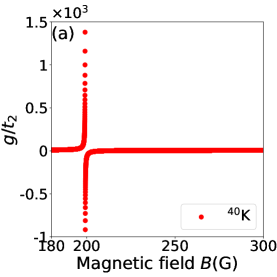
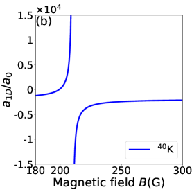
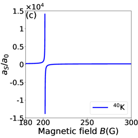
Figure S3: (a) Feshbach interaction strength $g$ as a function of the magnetic field for ⁴⁰K atoms. (b) Effective one-dimensional $S$-wave scattering length $a_{1D}$ as a function of the magnetic field for ⁴⁰K atoms. (c) Three-dimensional $S$-wave scattering length $a_{S}$ as a function of the magnetic field for ⁴⁰K atoms. The experimental parameters are given by $t_{2}=(2\pi)\times 1000$ Hz Atala2013np , $\omega_{\perp}=(2\pi)\times 2\times 10^{5}$ Hz Liao2010nature $B_{0}=202.1$G, $\Delta_{B}=8$G, $a_{\rm bg}=174a_{0}$ Regal2004prl ; Chin2010rmp with the Bohr radius $a_{0}$.

In order to investigate polaron physics in our setup, we consider Feshbach resonance interaction between majority spin-$\uparrow$ fermions and and a static impurity fermion with spin-$\downarrow$ in $s$ site of the $x_{0}$-th cell. Here, we choose $s=A$ in the main text, and there is analogous results if we had chosen $s=B$ instead.

As a result, atoms with spin-$\uparrow$ and spin-$\downarrow$ interact via an on-site interaction Hamiltonian $\hat{H}_{\rm Int}$ in $s$ site of the $x_{0}$-th cell

$$\hat{H}_{\rm int}=g\hat{b}_{x_{0},s}^{\dagger}\hat{b}_{x_{0},s}\hat{c}_{x_{0},s}^{\dagger}\hat{c}_{x_{0},s},$$ (S121)

where $\hat{b}_{x_{0},s}$ with $s=A/B$ is the annihilation field operator for the impurity atom in $s$ site of the $x_{0}$-th cell. The interaction coupling constant for a unit cell of size $d$ takes

$$g=g_{1D}/d,$$ (S122)

where

$$g_{1D}=-\frac{\hbar^{2}}{m_{r}a_{1D}},$$ (S123)

with the reduced mass $m_{r}=m/2$. Olshanii first obtained the atom-atom scattering under transverse harmonic confinement where the effective one-dimensional coupling strength $g_{1D}$ diverges at a particular ratio of the confinement and scattering lengths $a_{S}$ as shown in Eqs. (S124) and (S125). Hence the even-wave scattering length $a_{1D}$ (shown in Fig. S3(b)) in one dimension is Olshanii1998prl ; Olshanii2003prl ; Chin2010rmp ; Qin20201pra ; Qin20202pra

$$a_{1D}=-\frac{\ell^{2}_{\perp}}{2a_{S}}+\frac{{\cal C}\ell_{\perp}}{2},$$ (S124)

where ${\cal C}=1.4603$, $\ell_{\perp}=\sqrt{2\hbar/(m\omega_{\perp})}$, and $\omega_{\perp}$ is the transverse trapping frequency with $\omega_{\perp}=(2\pi)\times 2\times 10^{5}$ Hz in experiment Liao2010nature . This gives ${\cal C}\ell_{\perp}/2\approx 690.74a_{0}$. As shown in Fig. S3(c), near the resonance magnetic field $B_{0}=202.1$G, we have $a_{S}\gg{\cal C}\ell_{\perp}/2$. $a_{S}$ is the three-dimensional $S$-wave scattering length which is empirically fitted to be Chin2010rmp ; Regal2004prl

$$a_{S}=a_{\rm bg}\left(1-\frac{\Delta_{B}}{B-B_{0}}\right),$$ (S125)

where $a_{\rm bg}$ is the background scattering length, $B$ is the strength of the magnetic field, $B_{0}$ is the position of the Feshbach resonance, and $\Delta_{B}$ is the three-dimensional resonance width. For ⁴⁰K, we have $B_{0}=202.1$G, $\Delta_{B}=8$G, $a_{\rm bg}=174a_{0}$ with the Bohr radius $a_{0}$ Regal2004prl ; Chin2010rmp . As such, as shown in Fig. S3(a), when $B\rightarrow B_{0}$, $g$ does not diverge, but saturates at a large $\sim-17.88t_{2}$. When $B\rightarrow B_{c}\sim 200$G, $g$ saturates at a minimum $\sim-1000t_{2}$.

Appendix SII Additional data

SII.1 Energy spectra

SII.1.1 Energy spectra for minimal toy model $\hat{H}_{\rm min}$ under PBCs

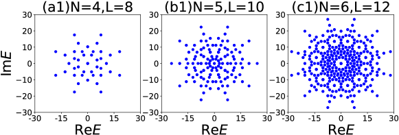
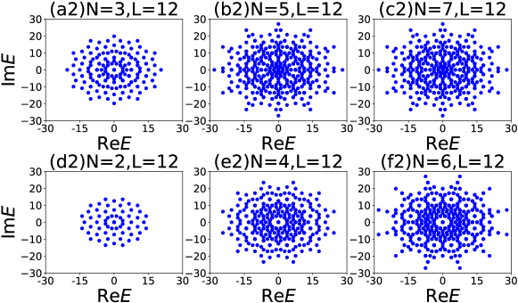
Figure S4: Energy spectra of $\hat{H}_{\text{min}}$ under PBCs for different number of fermions $N$ and sites $L$ with $\alpha=2$ and $g=0$. In general, the number of spikes is given by $L$. (a1-c1) Different system sizes $L$, all at half-filling. (a2-f2) Different number of fermions, at constant number of sites $L=12$, where (a2-c2) are for different odd number of fermions and (d2-f2) are for different even number of fermions.

In general, it is indicated from Fig. S4 that the number of spikes in the energy spectrum is given by the number of system sizes $L$.

SII.1.2 Energy spectra for cold-atom setup $\hat{H}$ under OBCs

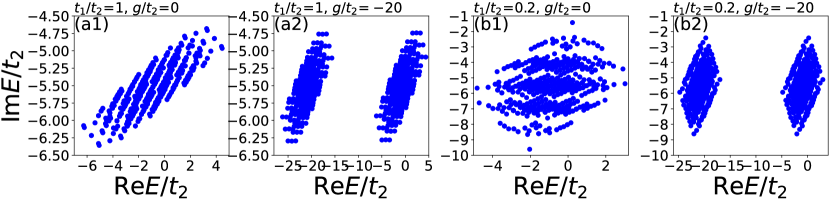
Figure S5: Energy spectra for Hamiltonian (SII.1.2) under OBCs with (a1): $t_{1}/t_{2}=1$ and $g=0$ (a2): $t_{1}/t_{2}=1$ and $g/t_{2}=-20$. (b1): $t_{1}/t_{2}=0.2$ and $g=0$. (b2) $t_{1}/t_{2}=0.2$ and $g/t_{2}=-20$. The other parameters are $t_{2}=(2\pi)\times 1000$ Hz Atala2013np , the impurity position is $x_{0}=1$ ($A$ site), and $\tilde{\gamma}/t_{2}=0.92-0.15i$ at half filling $N=6$ and $2L=12$. Noticeably, the effect of the local interaction $g$ is non-local, drastically affecting the entire spectrum whether under OBCs (shown here) or PBCs (see main text).

Our interacting Hamiltonian is given by

$$\hat{H} =\sum_{x=1}^{L}\left[-i\tilde{\gamma}(\hat{c}_{j,A}^{\dagger}\hat{c}_{j,A}+\hat{c}_{j,B}^{\dagger}\hat{c}_{j,B})+\left(t_{1}+\tilde{\gamma}\right)\hat{c}_{x,A}^{\dagger}\hat{c}_{x,B}+\left(t_{1}-\tilde{\gamma}\right)\hat{c}_{x,B}^{\dagger}\hat{c}_{x,A}\right]$$

$$~{}~{}+t_{2}\sum_{x=1}^{L-1}(\hat{c}_{x+1,A}^{\dagger}\hat{c}_{x,B}+{\rm H.c.})+g\hat{n}_{x_{0},s}^{(b)}\hat{n}_{x_{0},s},$$ (S126)

where $\hat{n}_{x_{0},s}=\hat{c}_{x_{0},s}^{\dagger}\hat{c}_{x_{0},s}$ is the number operator at site $s$ of cell $x_{0}$ for environment atoms. $\hat{n}_{x_{0},s}^{(b)}=\hat{b}_{x_{0},s}^{\dagger}\hat{b}_{x_{0},s}$ is the number operator at site $s$ of cell $x_{0}$ for impurity atom. In our exact diagonalization calculations, we consider the system with half filling condition (see Fig. S5).

To compare with the energy spectra under PBC in the main text, we plot the energy spectra under OBC as shown in Fig. S5. It is found that the impurity interaction can also non-perturbatively split the entire OBC energy spectrum into two halves as those under PBC.

SII.2 Spatial density

SII.2.1 Spatial density of the long-time steady state

In the fock space basis $\hat{F}=(\langle 1|,\langle 2|,...,\langle C_{2L}^{N}|)^{T}$, the number density operator at site $x$ is given by

$$\hat{n}_{\text{fock}}(x)=\hat{F}\hat{n}_{x}\hat{F}^{\dagger}=\left(\begin{array}[]{cccccc}\langle 1|\hat{n}_{x}|1\rangle&\langle 1|\hat{n}_{x}|2\rangle&\cdot\cdot\cdot&\langle 1|\hat{n}_{x}|C_{2L}^{N}\rangle\\ \langle 2|\hat{n}_{x}|1\rangle&\langle 2|\hat{n}_{x}|2\rangle&\cdot\cdot\cdot&\langle 2|\hat{n}_{x}|C_{2L}^{N}\rangle\\ \cdot\cdot\cdot&\cdot\cdot\cdot&\cdot\cdot\cdot&\cdot\cdot\cdot\\ \langle C_{2L}^{N}|\hat{n}_{x}|1\rangle&\langle C_{2L}^{N}|\hat{n}_{x}|2\rangle&\cdot\cdot\cdot&\langle C_{2L}^{N}|\hat{n}_{x}|C_{2L}^{N}\rangle\end{array}\right),$$ (S131)

where $\hat{n}_{x}=\hat{c}_{x}^{\dagger}\hat{c}_{x}$.

We define the spatial density of the long-time steady state (see the time evolutions in Figs. S6 and S7)

$$\rho(x)\equiv\lim_{t\to\infty}\langle\psi^{R}(t)|\hat{n}_{x}|\psi^{R}(t)\rangle,$$ (S132)

where $|\psi^{R}(t)\rangle=e^{-i\hat{H}t}\left|\psi^{R}(0)\right\rangle/\left\|\left|e^{-i\hat{H}t}\psi^{R}(t)\right\rangle\right\|$ which is the state under quench dynamics of a prepared initial state $\left|\psi^{R}(0)\right\rangle=(\left|1010\cdots\right\rangle+\left|0101\cdots\right\rangle)/\sqrt{2}$ with the Hamiltonian $\hat{H}$. We choose the final state to be after a sufficiently long-time evolution such that the spatial density reaches a steady configuration.

To understand the steady state obtained under non-Hermitian time evolution, we consider an initial state expressed in eigenvalue basis $|\psi(0)\rangle=\sum_{n}c_{n}\left|E_{n}\right\rangle$, and express the time dynamics as

$$e^{-i\hat{H}t}|\psi(0)\rangle=\sum_{n}e^{-ic_{n}{\rm Re}(E_{n})t+c_{n}{\rm Im}(E_{n})t}\left|E_{n}\right\rangle.$$ (S133)

Thus, long-time dynamics will converge to the eigenstate with the largest imaginary part of the eigenvalue:

$$\lim_{t\to\infty}e^{-i\hat{H}t}|\psi(0)\rangle\rightarrow\left|{\rm Max}\,{\rm Im}(E_{n})\right\rangle.$$ (S134)

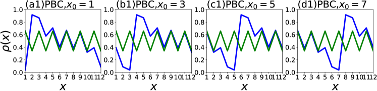
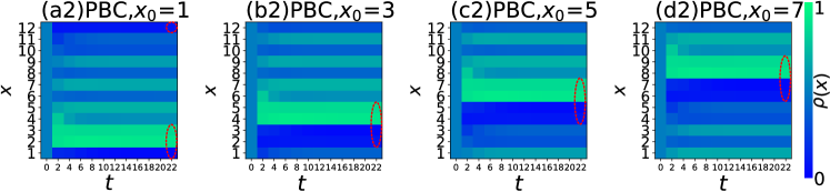
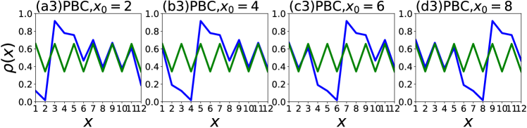
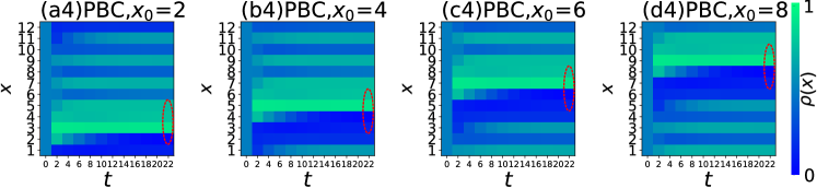
Figure S6: (a1-d1) Long-time steady-state spatial density in Eq. (S132) under PBCs for different odd impurity positions $x_{0}=1,3,5,7$ respectively. Note its translation invariant profile, which is exhibits the characteristic antisymmetric squeezed polaron profile (blue) for $g/t_{2}=-10$, or reference non-interacting case (green) with $g=0$. Parameters are $t_{1}/t_{2}=1$ at half filling $N=6$ and $2L=12$, $\tilde{\gamma}/t_{2}=0.92-0.15i$, $t_{2}=(2\pi)\times 1000$ Hz Atala2013np , and the evolution time is in units of $t_{2}$. (a2-d2) Dynamics of the spatial density along the lattice for different odd impurity positions $x_{0}=1,3,5,7$ respectively with $g/t_{2}=-10$. (a3-d3) Long-time steady-state spatial density in Eq. (S132) under PBCs for different even impurity positions $x_{0}=2,4,6,8$ respectively. (a4-d4) Dynamics of the spatial density along the lattice for different even impurity positions $x_{0}=2,4,6,8$ respectively with $g/t_{2}=-10$. Here, the initial state is $\left|\psi^{R}(0)\right\rangle=(\left|101010101010\right\rangle+\left|010101010101\right\rangle)/\sqrt{2}$. The antisymmetric dipole-like squeezed polaron (red circled) emerges after a short time, and persists in the steady state.

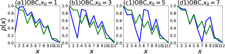
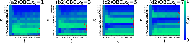
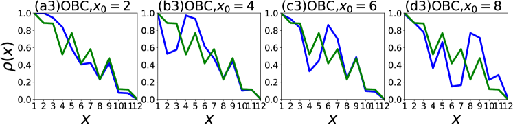
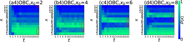
Figure S7: (a1-d1) Long-time steady-state spatial density in Eq. (S132) under OBCs for different odd impurity positions $x_{0}=1,3,5,7$ respectively. (a2-d2) Dynamics of the spatial density along the lattice for different odd impurity positions $x_{0}=1,3,5,7$ respectively with $g/t_{2}=-10$. (a3-d3) Long-time steady-state spatial density in Eq. (S132) under OBCs for different even impurity positions $x_{0}=2,4,6,8$ respectively. (a4-d4) Dynamics of the spatial density along the lattice for different even impurity positions $x_{0}=2,4,6,8$ respectively with $g/t_{2}=-10$. The other parameters are the same with Fig. S6. Note that even though finite-size effects become more prominent due to the boundaries, the characteristic antisymmetric dipole-like squeezed polaron profile (red circled) can still be seen, independent of the inevitable non-Hermitian skin effect at the $x=1$ boundary.

Comparing Figs. S6 and S7, one can find that in the even-site impurity position cases, there is one-site shift for the squeezed polaron between PBC and OBC. But in the odd-site impurity position cases, there is no such shift for the squeezed polaron between PBC and OBC. This is a sublattice effect. Furthermore, Fig. S7 shows that even though finite-size effects become more prominent due to the boundaries, the characteristic antisymmetric dipole-like squeezed polaron profile (red circled) can still be seen, independent of the inevitable non-Hermitian skin effect at the $x=1$ boundary.

SII.2.2 Spatial density in a dynamical quench

In order to investigate the necessity of the confluence of non-Hermiticity, non-reciprocity, and impurity interaction for observing squeezed polarons, we consider quench dynamics on spatial density with different impurity interaction strengths in our cold-atom experimental proposal model Hamiltonian (Eq. (5) in the main text). We activate the dissipation at a specific time:

$$\hat{H}(t)=\begin{cases}\hat{H}_{\tilde{\gamma}=0},&(0\leqslant t<t_{c});\\ \hat{H}_{\tilde{\gamma}\neq 0},&(t\geqslant t_{c}),\end{cases}$$ (S135)

where $t_{c}$ is the time when the quench is added, and $\hat{H}$ is the Hamiltonian in Eq. (SII.1.2).

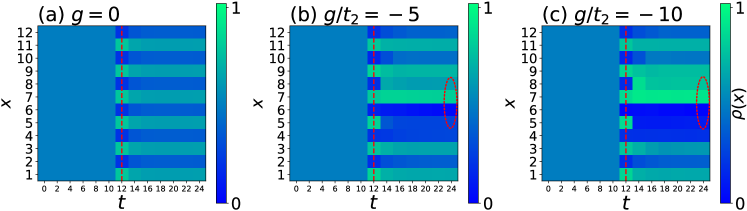
Figure S8: Quench dynamics according to Eq. (S135) under PBCs such that we activate the dissipative loss at $t_{c}$ (red dashed line) for (a) $g=0$, (b) $g/t_{2}=-5$, and (c) $g/t_{2}=-10$. We set the impurity position $x_{0}=6$ ($B$ site), $\tilde{\gamma}/t_{2}=0.92-0.15i$, $t_{1}/t_{2}=1$ with $N=6$ fermions in $2L=12$ sites, and prepare the initial state as $\ket{\psi^{R}(0)}=(\ket{101010101010}+\ket{010101010101})/\sqrt{2}$. Evidently, the antisymmetric dipole-like squeezed polaron profiles (red circled) do not appear until after the non-Hermitian dissipation is switched on, even for the case with nonzero $g$. This shows that Hermitian polarons do not manifest in the time-evolution of the given initial state (and in fact most other initial states that are not ground states), unlike non-Hermitian polarons which universally appear as a long-time steady-state property. For $g=0$, there is spatial density only alternates between even and odd sites, without assuming any distinct antisymmetric profile.

As shown in the above three Figs. S8(a,b,c), for $0<t<t_{c}$ without the non-Hermiticity and non-reciprocity, the spatial density always equals to $1/2$ which means that there is no squeezed polarons. Besides, it indicates from Fig. S8(a) that the squeezed polarons also cannot be formed without impurity interaction. This demonstrates a very important point: while Hermitian polarons only manifest in the ground state, non-Hermitian polaron behavior, i.e., asymmetric dipole-like accumulation is much more universal, appearing almost universally in the long-time steady-state behavior.

Indeed, our squeezed polarons are interesting dipole-like accumulations of fermionic density that only exist when all the three ingredients: non-Hermiticity, non-reciprocity, and impurity interaction, are simultaneously present.

Besides, we can also consider the quench dynamics with impurity interaction suddenly being turned on at a specific time $t_{c}$:

$$\hat{H}(t)=\begin{cases}\hat{H}_{g=0},&(0\leqslant t<t_{c});\\ \hat{H}_{g\neq 0},&(t\geqslant t_{c}),\end{cases}$$ (S136)

where $\hat{H}$ is the Hamiltonian in Eq. (SII.1.2).

Figure S9: Quench dynamics in Eq. (S136) under PBCs such that we activate the impurity interaction at $t_{c}$ (red dashed line) for (a) $\tilde{\gamma}=0$ and (b) $\tilde{\gamma}/t_{2}=0.92-0.15i$. We set the impurity position $x_{0}=6$ ($B$ site), $g/t_{2}=-10$, $t_{1}/t_{2}=1$ with $N=6$ fermions in $2L=12$ sites, and prepare the initial state as $\ket{\psi^{R}(0)}=(\ket{101010101010}+\ket{010101010101})/\sqrt{2}$. Evidently, the squeezed polaron (red circled) only exists for $\tilde{\gamma}\neq 0$, and also after the impurity interaction $g$ is turned on.

As shown in Fig. S9(a), for the Hermitian case, no matter adding impurity interaction or not, the spatial density always equals to $1/2$ which means that there is no squeezed polarons. Besides, it is indicated from Fig. S9(b) that, for the non-Hermitian case, the squeezed polarons also cannot be formed without impurity interaction. Therefore, our squeezed polarons only exist when all the three ingredients: non-Hermiticity, non-reciprocity, and impurity interaction, are simultaneously present.

References

(1)
L. Feng, M. Ayache, J. Huang, Y.-L. Xu, M.-H. Lu, Y.-F. Chen, Y. Fainman, and
A. Scherer, “Nonreciprocal light propagation in a silicon photonic
circuit,” Science, vol. 333, no. 6043, pp. 729–733, 2011.
(2)
Z. Shen, Y.-L. Zhang, Y. Chen, C.-L. Zou, Y.-F. Xiao, X.-B. Zou, F.-W. Sun,
G.-C. Guo, and C.-H. Dong, “Experimental realization of optomechanically
induced non-reciprocity,” Nature Photonics, vol. 10, no. 10, p. 657,
2016.
(3)
S. H. Park, S.-G. Lee, S. Baek, T. Ha, S. Lee, B. Min, S. Zhang, M. Lawrence,
and T.-T. Kim, “Observation of an exceptional point in a non-hermitian
metasurface,” Nanophotonics, vol. 9, no. 5, pp. 1031–1039, 2020.
(4)
C. Coulais, D. Sounas, and A. Alù, “Static non-reciprocity in mechanical
metamaterials,” Nature, vol. 542, no. 7642, p. 461, 2017.
(5)
W. Zhu, X. Fang, D. Li, Y. Sun, Y. Li, Y. Jing, and H. Chen, “Simultaneous
observation of a topological edge state and exceptional point in an open and
non-hermitian acoustic system,” Physical review letters, vol. 121,
no. 12, p. 124501, 2018.
(6)
A. Ghatak, M. Brandenbourger, J. van Wezel, and C. Coulais, “Observation of
non-hermitian topology and its bulk–edge correspondence in an active
mechanical metamaterial,” Proceedings of the National Academy of
Sciences, vol. 117, no. 47, pp. 29561–29568, 2020.
(7)
M. Brandenbourger, X. Locsin, E. Lerner, and C. Coulais, “Non-reciprocal
robotic metamaterials,” Nature communications, vol. 10, no. 1,
pp. 1–8, 2019.
(8)
H. Gao, H. Xue, Z. Gu, T. Liu, J. Zhu, and B. Zhang, “Non-hermitian route to
higher-order topology in an acoustic crystal,” Nature communications,
vol. 12, no. 1888, pp. 1–7, 2021.
(9)
T. Helbig, T. Hofmann, S. Imhof, M. Abdelghany, T. Kiessling, L. Molenkamp,
C. Lee, A. Szameit, M. Greiter, and R. Thomale, “Generalized bulk–boundary
correspondence in non-hermitian topolectrical circuits,” Nature
Physics, vol. 16, no. 7, pp. 747–750, 2020.
(10)
T. Hofmann, T. Helbig, C. H. Lee, M. Greiter, and R. Thomale, “Chiral voltage
propagation and calibration in a topolectrical chern circuit,” Physical
review letters, vol. 122, no. 24, p. 247702, 2019.
(11)
S. Liu, S. Ma, C. Yang, L. Zhang, W. Gao, Y. J. Xiang, T. J. Cui, and S. Zhang,
“Gain-and loss-induced topological insulating phase in a non-hermitian
electrical circuit,” Physical Review Applied, vol. 13, no. 1,
p. 014047, 2020.
(12)
T. Hofmann, T. Helbig, F. Schindler, N. Salgo, M. Brzezińska, M. Greiter,
T. Kiessling, D. Wolf, A. Vollhardt, A. Kabaši, et al.,
“Reciprocal skin effect and its realization in a topolectrical circuit,”
Physical Review Research, vol. 2, no. 2, p. 023265, 2020.
(13)
S. Liu, R. Shao, S. Ma, L. Zhang, O. You, H. Wu, Y. J. Xiang, T. J. Cui, and
S. Zhang, “Non-hermitian skin effect in a non-hermitian electrical
circuit,” Research, vol. 2021, no. 5608038, 2021.
(14)
D. Zou, T. Chen, W. He, J. Bao, C. H. Lee, H. Sun, and X. Zhang, “Observation
of hybrid higher-order skin-topological effect in non-hermitian topolectrical
circuits,” Nature Communications, vol. 12, no. 7201, pp. 1–11, 2021.
(15)
A. Stegmaier, S. Imhof, T. Helbig, T. Hofmann, C. H. Lee, M. Kremer,
A. Fritzsche, T. Feichtner, S. Klembt, S. Höfling, et al.,
“Topological defect engineering and p t symmetry in non-hermitian electrical
circuits,” Physical Review Letters, vol. 126, no. 21, p. 215302, 2021.
(16)
C. Shang, S. Liu, R. Shao, P. Han, X. Zang, X. Zhang, K. N. Salama, W. Gao,
C. H. Lee, R. Thomale, A. Manchon, S. Zhang, T. J. Cui, and
U. Schwingenschlögl, “Experimental identification of the second-order
non-hermitian skin effect with physics-graph-informed machine learning,”
Advanced Science, vol. n/a, no. n/a, p. 2202922.
(17)
L. Xiao, T. Deng, K. Wang, G. Zhu, Z. Wang, W. Yi, and P. Xue, “Non-hermitian
bulk–boundary correspondence in quantum dynamics,” Nature Physics,
vol. 16, p. 761, 2020.
(18)
L. Feng, R. El-Ganainy, and L. Ge, “Non-hermitian photonics based on
parity–time symmetry,” Nature Photonics, vol. 11, no. 12, p. 752,
2017.
(19)
L. D. Tzuang, K. Fang, P. Nussenzveig, S. Fan, and M. Lipson, “Non-reciprocal
phase shift induced by an effective magnetic flux for light,” Nature
photonics, vol. 8, no. 9, p. 701, 2014.
(20)
H. Zhou, C. Peng, Y. Yoon, C. W. Hsu, K. A. Nelson, L. Fu, J. D. Joannopoulos,
M. Soljačić, and B. Zhen, “Observation of bulk fermi arc and
polarization half charge from paired exceptional points,” Science,
vol. 359, no. 6379, pp. 1009–1012, 2018.
(21)
B. Zhen, C. W. Hsu, Y. Igarashi, L. Lu, I. Kaminer, A. Pick, S.-L. Chua, J. D.
Joannopoulos, and M. Soljačić, “Spawning rings of exceptional
points out of dirac cones,” Nature, vol. 525, no. 7569, p. 354, 2015.
(22)
J. M. Zeuner, M. C. Rechtsman, Y. Plotnik, Y. Lumer, S. Nolte, M. S. Rudner,
M. Segev, and A. Szameit, “Observation of a topological transition in the
bulk of a non-hermitian system,” Physical Review Letters, vol. 115,
p. 040402, Jul 2015.
(23)
M.-A. Miri and A. Alù, “Exceptional points in optics and photonics,” Science, vol. 363, no. 6422, p. eaar7709, 2019.
(24)
J. Li, A. K. Harter, J. Liu, L. de Melo, Y. N. Joglekar, and L. Luo,
“Observation of parity-time symmetry breaking transitions in a dissipative
floquet system of ultracold atoms,” Nat. Comm., vol. 10, no. 1,
p. 855, 2019.
(25)
S. Lapp, F. A. An, B. Gadway, et al., “Engineering tunable local loss in
a synthetic lattice of momentum states,” New Journal of Physics,
vol. 21, no. 4, p. 045006, 2019.
(26)
Z. Ren, D. Liu, E. Zhao, C. He, K. K. Pak, J. Li, and G.-B. Jo, “Chiral
control of quantum states in non-hermitian spin–orbit-coupled fermions,”
Nature Physics, vol. 18, no. 4, pp. 385–389, 2022.
(27)
Q. Liang, D. Xie, Z. Dong, H. Li, H. Li, B. Gadway, W. Yi, and B. Yan,
“Dynamic signatures of non-hermitian skin effect and topology in ultracold
atoms,” Physical Review Letters, vol. 129, no. 7, p. 070401, 2022.
(28)
W. Yi, “An exceptional mass dance,” Nature Physics, vol. 18, no. 4,
pp. 370–371, 2022.
(29)
W. Gou, T. Chen, D. Xie, T. Xiao, T.-S. Deng, B. Gadway, W. Yi, and B. Yan,
“Tunable nonreciprocal quantum transport through a dissipative aharonov-bohm
ring in ultracold atoms,” Phys. Rev. Lett., vol. 124, p. 070402, Feb
2020.
(30)
E. J. Bergholtz, J. C. Budich, and F. K. Kunst, “Exceptional topology of
non-hermitian systems,” Rev. Mod. Phys., vol. 93, p. 015005, Feb 2021.
(31)
E. Lafalce, Q. Zeng, C. H. Lin, M. J. Smith, S. T. Malak, J. Jung, Y. J. Yoon,
Z. Lin, V. V. Tsukruk, and Z. V. Vardeny, “Robust lasing modes in coupled
colloidal quantum dot microdisk pairs using a non-hermitian exceptional
point,” Nature communications, vol. 10, no. 1, pp. 1–8, 2019.
(32)
V. Kozii and L. Fu, “Non-hermitian topological theory of finite-lifetime
quasiparticles: prediction of bulk fermi arc due to exceptional point,” arXiv preprint arXiv:1708.05841, 2017.
(33)
T. Yoshida and Y. Hatsugai, “Exceptional rings protected by emergent symmetry
for mechanical systems,” Physical Review B, vol. 100, no. 5,
p. 054109, 2019.
(34)
T. Yoshida, R. Peters, N. Kawakami, and Y. Hatsugai, “Symmetry-protected
exceptional rings in two-dimensional correlated systems with chiral
symmetry,” Physical Review B, vol. 99, no. 12, p. 121101, 2019.
(35)
R. Okugawa and T. Yokoyama, “Topological exceptional surfaces in non-hermitian
systems with parity-time and parity-particle-hole symmetries,” Physical
Review B, vol. 99, no. 4, p. 041202, 2019.
(36)
H. Hodaei, A. U. Hassan, S. Wittek, H. Garcia-Gracia, R. El-Ganainy, D. N.
Christodoulides, and M. Khajavikhan, “Enhanced sensitivity at higher-order
exceptional points,” Nature, vol. 548, no. 7666, pp. 187–191, 2017.
(37)
D. Heiss, “Circling exceptional points,” Nature Physics, vol. 12,
no. 9, pp. 823–824, 2016.
(38)
W. Heiss, “The physics of exceptional points,” Journal of Physics A:
Mathematical and Theoretical, vol. 45, no. 44, p. 444016, 2012.
(39)
Z. Gong, Y. Ashida, K. Kawabata, K. Takasan, S. Higashikawa, and M. Ueda,
“Topological phases of non-hermitian systems,” Physical Review X,
vol. 8, no. 3, p. 031079, 2018.
(40)
T. Yoshida, R. Peters, and N. Kawakami, “Non-hermitian perspective of the band
structure in heavy-fermion systems,” Physical Review B, vol. 98,
no. 3, p. 035141, 2018.
(41)
K. Zhang, Z. Yang, and C. Fang, “Correspondence between winding numbers and
skin modes in non-hermitian systems,” Physical Review Letters,
vol. 125, no. 12, p. 126402, 2020.
(42)
Q. Zhong, M. Khajavikhan, D. N. Christodoulides, and R. El-Ganainy, “Winding
around non-hermitian singularities,” Nature communications, vol. 9,
no. 1, pp. 1–9, 2018.
(43)
S. Rafi-Ul-Islam, Z. B. Siu, and M. B. Jalil, “Topological phases with higher
winding numbers in nonreciprocal one-dimensional topolectrical circuits,”
Physical Review B, vol. 103, no. 3, p. 035420, 2021.
(44)
T. Yoshida, T. Mizoguchi, and Y. Hatsugai, “Mirror skin effect and its
electric circuit simulation,” Phys. Rev. Res., vol. 2, p. 022062, Jun
2020.
(45)
G. Sun, J.-C. Tang, and S.-P. Kou, “Biorthogonal quantum criticality in
non-hermitian many-body systems,” Frontiers of Physics, vol. 17,
no. 3, pp. 1–9, 2022.
(46)
W. Xi, Z.-H. Zhang, Z.-C. Gu, and W.-Q. Chen, “Classification of topological
phases in one dimensional interacting non-hermitian systems and emergent
unitarity,” Science Bulletin, 2021.
(47)
C. H. Lee, L. Li, R. Thomale, and J. Gong, “Unraveling non-hermitian pumping:
emergent spectral singularities and anomalous responses,” Physical
Review B, vol. 102, no. 8, p. 085151, 2020.
(48)
L. Li and C. H. Lee, “Non-hermitian pseudo-gaps,” Science Bulletin,
vol. 67, no. 7, pp. 685–690, 2022.
(49)
L. Li, C. H. Lee, S. Mu, and J. Gong, “Critical non-hermitian skin effect,”
Nature communications, vol. 11, no. 1, pp. 1–8, 2020.
(50)
P.-Y. Chang, J.-S. You, X. Wen, and S. Ryu, “Entanglement spectrum and entropy
in topological non-hermitian systems and nonunitary conformal field theory,”
Physical Review Research, vol. 2, no. 3, p. 033069, 2020.
(51)
C. H. Lee, “Exceptional bound states and negative entanglement entropy,” Physical Review Letters, vol. 128, no. 1, p. 010402, 2022.
(52)
N. Okuma and M. Sato, “Quantum anomaly, non-hermitian skin effects, and
entanglement entropy in open systems,” Physical Review B, vol. 103,
no. 8, p. 085428, 2021.
(53)
S. Yao and Z. Wang, “Edge states and topological invariants of non-hermitian
systems,” Physical review letters, vol. 121, no. 8, p. 086803, 2018.
(54)
Y. Xiong, “Why does bulk boundary correspondence fail in some non-hermitian
topological models,” Journal of Physics Communications, vol. 2, no. 3,
p. 035043, 2018.
(55)
C. H. Lee and R. Thomale, “Anatomy of skin modes and topology in non-hermitian
systems,” Physical Review B, vol. 99, p. 201103, May 2019.
(56)
F. K. Kunst, E. Edvardsson, J. C. Budich, and E. J. Bergholtz, “Biorthogonal
bulk-boundary correspondence in non-hermitian systems,” Phys. Rev.
Lett., vol. 121, p. 026808, Jul 2018.
(57)
K. Yokomizo and S. Murakami, “Non-bloch band theory of non-hermitian
systems,” Phys. Rev. Lett., vol. 123, p. 066404, Aug 2019.
(58)
K.-I. Imura and Y. Takane, “Generalized bulk-edge correspondence for
non-hermitian topological systems,” Phys. Rev. B, vol. 100, p. 165430,
Oct 2019.
(59)
L. Jin and Z. Song, “Bulk-boundary correspondence in a non-hermitian system in
one dimension with chiral inversion symmetry,” Physical Review B,
vol. 99, p. 081103, Feb 2019.
(60)
D. S. Borgnia, A. J. Kruchkov, and R.-J. Slager, “Non-hermitian boundary modes
and topology,” Physical review letters, vol. 124, no. 5, p. 056802,
2020.
(61)
L. Li, S. Mu, C. H. Lee, and J. Gong, “Quantized classical response from
spectral winding topology,” Nature communications, vol. 12, no. 1,
pp. 1–11, 2021.
(62)
C. Lv, R. Zhang, and Q. Zhou, “Curving the space by non-hermiticity,” arXiv preprint arXiv:2106.02477, 2021.
(63)
R. Yang, J. W. Tan, T. Tai, J. M. Koh, L. Li, S. Longhi, and C. H. Lee,
“Designing non-hermitian real spectra through electrostatics,” arXiv
preprint arXiv:2201.04153, 2022.
(64)
H. Jiang and C. H. Lee, “Dimensional transmutation from non-hermiticity,”
arXiv preprint arXiv:2207.08843, 2022.
(65)
T. Tai and C. H. Lee, “Zoology of non-hermitian spectra and their graph
topology,” arXiv preprint arXiv:2202.03462, 2022.
(66)
R. Hamazaki, K. Kawabata, and M. Ueda, “Non-hermitian many-body
localization,” Phys. Rev. Lett., vol. 123, p. 090603, Aug 2019.
(67)
L.-J. Zhai, S. Yin, and G.-Y. Huang, “Many-body localization in a
non-hermitian quasiperiodic system,” Phys. Rev. B, vol. 102,
p. 064206, Aug 2020.
(68)
K. Suthar, Y.-C. Wang, Y.-P. Huang, H. H. Jen, and J.-S. You, “Non-hermitian
many-body localization with open boundaries,” Phys. Rev. B, vol. 106,
p. 064208, Aug 2022.
(69)
Y.-C. Wang, K. Suthar, H. Jen, Y.-T. Hsu, and J.-S. You, “Non-hermitian skin
effects on many-body localized and thermal phases,” arXiv preprint
arXiv:2210.12998, 2022.
(70)
M. Luo, “Skin effect and excitation spectral of interacting non-hermitian
system,” arXiv preprint arXiv:2001.00697, 2020.
(71)
D.-W. Zhang, Y.-L. Chen, G.-Q. Zhang, L.-J. Lang, Z. Li, and S.-L. Zhu, “Skin
superfluid, topological mott insulators, and asymmetric dynamics in an
interacting non-hermitian aubry-andré-harper model,” Phys. Rev. B,
vol. 101, p. 235150, Jun 2020.
(72)
T. Liu, J. J. He, T. Yoshida, Z.-L. Xiang, and F. Nori, “Non-hermitian
topological mott insulators in one-dimensional fermionic superlattices,”
Phys. Rev. B, vol. 102, p. 235151, Dec 2020.
(73)
L. Zhou and X. Cui, “Enhanced fermion pairing and superfluidity by an
imaginary magnetic field,” Iscience, vol. 14, pp. 257–263, 2019.
(74)
L. Zhou, W. Yi, and X. Cui, “Dissipation-facilitated molecules in a fermi gas
with non-hermitian spin-orbit coupling,” Phys. Rev. A, vol. 102,
p. 043310, Oct 2020.
(75)
J.-S. Pan, W. Yi, and J. Gong, “Emergent pt-symmetry breaking of collective
modes with topological critical phenomena,” Communications Physics,
vol. 4, no. 1, pp. 1–8, 2021.
(76)
C. H. Lee, “Many-body topological and skin states without open boundaries,”
Phys. Rev. B, vol. 104, p. 195102, Nov 2021.
(77)
R. Shen and C. H. Lee, “Non-hermitian skin clusters from strong
interactions,” Communications Physics, vol. 5, no. 1, pp. 1–11, 2022.
(78)
L. Pan, X. Chen, Y. Chen, and H. Zhai, “Non-hermitian linear response
theory,” Nature Physics, vol. 16, no. 7, pp. 767–771, 2020.
(79)
K. Kawabata, K. Shiozaki, and S. Ryu, “Many-body topology of non-hermitian
systems,” Physical Review B, vol. 105, no. 16, p. 165137, 2022.
(80)
K. Yamamoto, M. Nakagawa, K. Adachi, K. Takasan, M. Ueda, and N. Kawakami,
“Theory of non-hermitian fermionic superfluidity with a complex-valued
interaction,” Physical Review Letters, vol. 123, p. 123601, Sep 2019.
(81)
F. Alsallom, L. Herviou, O. V. Yazyev, and M. Brzezińska, “Fate of the
non-hermitian skin effect in many-body fermionic systems,” Physical
Review Research, vol. 4, no. 3, p. 033122, 2022.
(82)
S.-B. Zhang, M. M. Denner, T. c. v. Bzdušek,
M. A. Sentef, and T. Neupert, “Symmetry breaking and spectral structure of
the interacting hatano-nelson model,” Phys. Rev. B, vol. 106,
p. L121102, Sep 2022.
(83)
A. N. Poddubny, “Topologically bound states, non-hermitian skin effect and
flat bands, induced by two-particle interaction,” arXiv preprint
arXiv:2211.06043, 2022.
(84)
T. Yoshida and Y. Hatsugai, “Fate of exceptional points under interactions:
Reduction of topological classifications,” arXiv preprint
arXiv:2211.08895, 2022.
(85)
P. Weinberg and M. Bukov, “Quspin: a python package for dynamics and exact
diagonalisation of quantum many body systems part i: spin chains,” SciPost Physics, vol. 2, Feb 2017.
(86)
P. Weinberg and M. Bukov, “Quspin: a python package for dynamics and exact
diagonalisation of quantum many body systems. part ii: bosons, fermions and
higher spins,” SciPost Physics, vol. 7, Aug 2019.
(87)
A. Schirotzek, C.-H. Wu, A. Sommer, and M. W. Zwierlein, “Observation of fermi
polarons in a tunable fermi liquid of ultracold atoms,” Phys. Rev.
Lett., vol. 102, p. 230402, Jun 2009.
(88)
Y. Zhang, W. Ong, I. Arakelyan, and J. E. Thomas, “Polaron-to-polaron
transitions in the radio-frequency spectrum of a quasi-two-dimensional fermi
gas,” Phys. Rev. Lett., vol. 108, p. 235302, Jun 2012.
(89)
C. Kohstall, M. Zaccanti, M. Jag, A. Trenkwalder, P. Massignan, G. M. Bruun,
F. Schreck, and R. Grimm, “Metastability and coherence of repulsive polarons
in a strongly interacting fermi mixture,” Nature, vol. 485,
pp. 615–618, May 2012.
(90)
M. Koschorreck, D. Pertot, E. Vogt, B. Frohlich, M. Feld, and M. Kohl,
“Attractive and repulsive fermi polarons in two dimensions,” Nature,
vol. 485, pp. 619–622, May 2012.
(91)
M. Cetina, M. Jag, R. S. Lous, I. Fritsche, J. T. M. Walraven, R. Grimm,
J. Levinsen, M. M. Parish, R. Schmidt, M. Knap, and et al., “Ultrafast
many-body interferometry of impurities coupled to a fermi sea,” Science, vol. 354, pp. 96–99, Oct 2016.
(92)
F. Scazza, G. Valtolina, P. Massignan, A. Recati, A. Amico, A. Burchianti,
C. Fort, M. Inguscio, M. Zaccanti, and G. Roati, “Repulsive fermi polarons
in a resonant mixture of ultracold atoms,” Phys. Rev.
Lett., vol. 118, p. 083602, Feb 2017.
(93)
Z. Yan, P. B. Patel, B. Mukherjee, R. J. Fletcher, J. Struck, and M. W.
Zwierlein, “Boiling a unitary fermi liquid,” Phys. Rev. Lett.,
vol. 122, p. 093401, Mar 2019.
(94)
N. D. Oppong, L. Riegger, O. Bettermann, M. Höfer, J. Levinsen, M. M.
Parish, I. Bloch, and S. Fölling, “Observation of coherent multiorbital
polarons in a two-dimensional fermi gas,” Physical Review Letters,
vol. 122, no. 19, p. 193604, 2019.
(95)
G. Ness, C. Shkedrov, Y. Florshaim, O. K. Diessel, J. von Milczewski,
R. Schmidt, and Y. Sagi, “Observation of a smooth polaron-molecule
transition in a degenerate fermi gas,” Phys. Rev. X, vol. 10,
p. 041019, Oct 2020.
(96)
M.-G. Hu, M. J. Van de Graaff, D. Kedar, J. P. Corson, E. A. Cornell, and D. S.
Jin, “Bose polarons in the strongly interacting regime,” Phys. Rev.
Lett., vol. 117, p. 055301, Jul 2016.
(97)
N. B. Jorgensen, L. Wacker, K. T. Skalmstang, M. M. Parish, J. Levinsen, R. S.
Christensen, G. M. Bruun, and J. J. Arlt, “Observation of attractive and
repulsive polarons in a bose-einstein condensate,” Phys. Rev. Lett.,
vol. 117, p. 055302, Jul 2016.
(98)
Z. Z. Yan, Y. Ni, C. Robens, and M. W. Zwierlein, “Bose polarons near quantum
criticality,” Science, vol. 368, pp. 190–194, Apr 2020.
(99)
H. Hu, L. Jiang, H. Pu, Y. Chen, and X.-J. Liu, “Universal impurity-induced
bound state in topological superfluids,” Phys. Rev. Lett., vol. 110,
p. 020401, Jan 2013.
(100)
C. H. Lee and X.-L. Qi, “Lattice construction of pseudopotential hamiltonians
for fractional chern insulators,” Physical Review B, vol. 90, no. 8,
p. 085103, 2014.
(101)
C. H. Lee, Z. Papić, and R. Thomale, “Geometric construction of quantum
hall clustering hamiltonians,” Physical Review X, vol. 5, no. 4,
p. 041003, 2015.
(102)
F. Grusdt, N. Y. Yao, D. Abanin, M. Fleischhauer, and E. Demler,
“Interferometric measurements of many-body topological invariants using
mobile impurities,” Nature communications, vol. 7, no. 1, pp. 1–9,
2016.
(103)
A. Camacho-Guardian, N. Goldman, P. Massignan, and G. M. Bruun, “Dropping an
impurity into a chern insulator: A polaron view on topological matter,” Phys. Rev. B, vol. 99, p. 081105, Feb 2019.
(104)
D. Pimenov, A. Camacho-Guardian, N. Goldman, P. Massignan, G. M. Bruun, and
M. Goldstein, “Topological transport of mobile impurities,” Phys. Rev.
B, vol. 103, p. 245106, Jun 2021.
(105)
F. Qin, X. Cui, W. Yi, et al., “Polaron in a p+ i p fermi topological
superfluid,” Physical Review A, vol. 99, no. 3, p. 033613, 2019.
(106)
F. Chevy, “Universal phase diagram of a strongly interacting fermi gas with
unbalanced spin populations,” Phys. Rev. A, vol. 74, p. 063628, Dec
2006.
(107)
C. Lobo, A. Recati, S. Giorgini, and S. Stringari, “Normal state of a
polarized fermi gas at unitarity,” Phys. Rev. Lett., vol. 97,
p. 200403, Nov 2006.
(108)
R. Combescot, A. Recati, C. Lobo, and F. Chevy, “Normal state of highly
polarized fermi gases: Simple many-body approaches,” Phys. Rev. Lett.,
vol. 98, p. 180402, May 2007.
(109)
G. M. Bruun and P. Massignan, “Decay of polarons and molecules in a strongly
polarized fermi gas,” Phys. Rev. Lett., vol. 105, p. 020403, Jul 2010.
(110)
C. J. M. Mathy, M. M. Parish, and D. A. Huse, “Trimers, molecules, and
polarons in mass-imbalanced atomic fermi gases,” Phys. Rev. Lett.,
vol. 106, p. 166404, Apr 2011.
(111)
S. Zöllner, G. M. Bruun, and C. Pethick, “Polarons and molecules in a
two-dimensional fermi gas,” Physical Review A, vol. 83, no. 2,
p. 021603, 2011.
(112)
M. M. Parish, “Polaron-molecule transitions in a two-dimensional fermi gas,”
Physical Review A, vol. 83, no. 5, p. 051603, 2011.
(113)
J. Levinsen, P. Massignan, F. Chevy, and C. Lobo, “p-wave polaron,” Physical Review Letters, vol. 109, no. 7, p. 075302, 2012.
(114)
W. Yi and W. Zhang, “Molecule and polaron in a highly polarized
two-dimensional fermi gas with spin-orbit coupling,” Phys. Rev. Lett.,
vol. 109, p. 140402, Oct 2012.
(115)
M. M. Parish and J. Levinsen, “Highly polarized fermi gases in two
dimensions,” Phys. Rev. A, vol. 87, p. 033616, Mar 2013.
(116)
W. Yi and X. Cui, “Polarons in ultracold fermi superfluids,” Phys. Rev.
A, vol. 92, p. 013620, Jul 2015.
(117)
Y. Nishida, “Polaronic atom-trimer continuity in three-component fermi
gases,” Physical Review Letters, vol. 114, no. 11, p. 115302, 2015.
(118)
M. M. Parish and J. Levinsen, “Quantum dynamics of impurities coupled to a
fermi sea,” Physical Review B, vol. 94, no. 18, p. 184303, 2016.
(119)
A. Camacho-Guardian, L. A. Pena Ardila, T. Pohl, and G. M. Bruun, “Bipolarons
in a bose-einstein condensate,” Phys. Rev. Lett., vol. 121, p. 013401,
Jul 2018.
(120)
X. Cui, “Fermi polaron revisited: Polaron-molecule transition and
coexistence,” Physical Review A, vol. 102, no. 6, p. 061301, 2020.
(121)
R. Pessoa, S. A. Vitiello, and L. A. P. Ardila, “Finite-range effects in the
unitary fermi polaron,” Phys. Rev. A, vol. 104, p. 043313, Oct 2021.
(122)
L. A. P. Ardila, “Dynamical formation of polarons in a bose-einstein
condensate: A variational approach,” Phys. Rev. A, vol. 103,
p. 033323, Mar 2021.
(123)
K. Seetharam, Y. Shchadilova, F. Grusdt, M. B. Zvonarev, and E. Demler,
“Dynamical quantum cherenkov transition of fast impurities in quantum
liquids,” Physical review letters, vol. 127, no. 18, p. 185302, 2021.
(124)
K. Seetharam, Y. Shchadilova, F. Grusdt, M. Zvonarev, and E. Demler, “Quantum
cherenkov transition of finite momentum bose polarons,” arXiv preprint
arXiv:2109.12260, 2021.
(125)
H. Hu, J. Wang, J. Zhou, and X.-J. Liu, “Crossover polarons in a strongly
interacting fermi superfluid,” Physical Review A, vol. 105, no. 2,
p. 023317, 2022.
(126)
F. Qin, C. H. Lee, R. Chen, et al., “Light-induced phase crossovers in a
quantum spin hall system,” Physical Review B, vol. 106, no. 23,
p. 235405, 2022.
(127)
F. Qin, R. Chen, and H.-Z. Lu, “Phase transitions in intrinsic magnetic
topological insulator with high-frequency pumping,” Journal of Physics:
Condensed Matter, vol. 34, no. 22, p. 225001, 2022.
(128)
F. Qin, S. Li, Z. Du, C. Wang, W. Zhang, D. Yu, H.-Z. Lu, X. Xie, et al.,
“Theory for the charge-density-wave mechanism of 3d quantum hall effect,”
Physical Review Letters, vol. 125, no. 20, p. 206601, 2020.
(129)
L. Li, C. H. Lee, and J. Gong, “Impurity induced scale-free localization,”
Communications Physics, vol. 4, no. 1, pp. 1–9, 2021.
(130)
M. Z. Hasan and C. L. Kane, “Colloquium: Topological insulators,” Rev.
Mod. Phys., vol. 82, pp. 3045–3067, Nov 2010.
(131)
C.-K. Chiu, J. C. Y. Teo, A. P. Schnyder, and S. Ryu, “Classification of
topological quantum matter with symmetries,” Rev. Mod. Phys., vol. 88,
p. 035005, Aug 2016.
(132)
For a more practical implementation involving physical flux, see the more
realistic cold-atom Hamiltonian presented later.
(133)Supplemental Materials.
(134)
N. Hatano and D. R. Nelson, “Localization transitions in non-hermitian quantum
mechanics,” Phys. Rev. Lett., vol. 77, pp. 570–573, Jul 1996.
(135)
N. Hatano and D. R. Nelson, “Vortex pinning and non-hermitian quantum
mechanics,” Phys. Rev. B, vol. 56, pp. 8651–8673, Oct 1997.
(136)
N. Hatano and D. R. Nelson, “Non-hermitian delocalization and
eigenfunctions,” Phys. Rev. B, vol. 58, pp. 8384–8390, Oct 1998.
(137)
S. Hikami, “Localization length and inverse participation ratio of two
dimensional electron in the quantized hall effect,” Progress of
theoretical physics, vol. 76, no. 6, pp. 1210–1221, 1986.
(138)
This is because a randomly given initial state would most likely overlap with
some of the many eigenstates in the right (reddish) cluster of Fig. 2(d1).
(139)
Y.-a. Liao, A. S. C. Rittner, T. Paprotta, W. Li, G. B. Partridge, R. G. Hulet,
S. K. Baur, and E. J. Mueller, “Spin-imbalance in a one-dimensional fermi
gas,” Nature, vol. 467, pp. 567–569, Sep 2010.
(140)
C. A. Regal, M. Greiner, and D. S. Jin, “Observation of resonance condensation
of fermionic atom pairs,” Phys. Rev. Lett., vol. 92, p. 040403, Jan
2004.
(141)
C. Chin, R. Grimm, P. Julienne, and E. Tiesinga, “Feshbach resonances in
ultracold gases,” Rev. Mod. Phys., vol. 82, pp. 1225–1286, Apr 2010.
(142)
M. Atala, M. Aidelsburger, J. T. Barreiro, D. Abanin, T. Kitagawa, E. Demler,
and I. Bloch, “Direct measurement of the zak phase in topological bloch
bands,” Nature Physics, vol. 9, pp. 795–800, Nov 2013.
(143)
M. Olshanii, “Atomic scattering in the presence of an external confinement and
a gas of impenetrable bosons,” Phys. Rev. Lett., vol. 81,
pp. 938–941, Aug 1998.
(144)
T. Bergeman, M. G. Moore, and M. Olshanii, “Atom-atom scattering under
cylindrical harmonic confinement: Numerical and analytic studies of the
confinement induced resonance,” Phys. Rev. Lett., vol. 91, p. 163201,
Oct 2003.
(145)
F. Qin, P. Zhang, and P.-L. Zhao, “Large-momentum tail of one-dimensional
fermi gases with spin-orbit coupling,” Phys. Rev. A, vol. 101,
p. 063619, Jun 2020.
(146)
F. Qin and P. Zhang, “Universal relations for hybridized - and -wave
interactions from spin-orbital coupling,” Phys. Rev. A, vol. 102,
p. 043321, Oct 2020.
(147)
C. A. Regal, C. Ticknor, J. L. Bohn, and D. S. Jin, “Tuning -wave
interactions in an ultracold fermi gas of atoms,” Phys. Rev. Lett.,
vol. 90, p. 053201, Feb 2003.
(148)
F. Qin, X. Cui, and W. Yi, “Universal relations and normal phase of an
ultracold fermi gas with coexisting - and -wave interactions,” Phys. Rev. A, vol. 94, p. 063616, Dec 2016.
(149)
F. Qin, J.-S. Pan, S. Wang, and G.-C. Guo, “Width of the confinement-induced
resonance in a quasi-one-dimensional trap with transverse anisotropy,” The European Physical Journal D, vol. 71, p. 304, Nov 2017.
(150)
In practice, at very strong resonance, the scattering length diverges and a
quantum halo state is formed instead.
(151)
Y.-J. Lin, R. L. Compton, A. R. Perry, W. D. Phillips, J. V. Porto, and I. B.
Spielman, “Bose-einstein condensate in a uniform light-induced vector
potential,” Phys. Rev. Lett., vol. 102, p. 130401, Mar 2009.
(152)
Y.-J. Lin, K. Jimenez-Garcia, and I. B. Spielman, “Spin-orbit-coupled
bose-einstein condensates,” Nature, vol. 471, pp. 83–86, Mar 2011.
(153)
J.-Y. Zhang, S.-C. Ji, Z. Chen, L. Zhang, Z.-D. Du, B. Yan, G.-S. Pan, B. Zhao,
Y.-J. Deng, H. Zhai, S. Chen, and J.-W. Pan, “Collective dipole oscillations
of a spin-orbit coupled bose-einstein condensate,” Phys. Rev. Lett.,
vol. 109, p. 115301, Sep 2012.
(154)
P. Wang, Z.-Q. Yu, Z. Fu, J. Miao, L. Huang, S. Chai, H. Zhai, and J. Zhang,
“Spin-orbit coupled degenerate fermi gases,” Phys. Rev. Lett.,
vol. 109, p. 095301, Aug 2012.
(155)
L. W. Cheuk, A. T. Sommer, Z. Hadzibabic, T. Yefsah, W. S. Bakr, and M. W.
Zwierlein, “Spin-injection spectroscopy of a spin-orbit coupled fermi gas,”
Phys. Rev. Lett., vol. 109, p. 095302, Aug 2012.
(156)
C. Qu, C. Hamner, M. Gong, C. Zhang, and P. Engels, “Observation of
zitterbewegung in a spin-orbit-coupled bose-einstein condensate,” Phys.
Rev. A, vol. 88, p. 021604, Aug 2013.
(157)
L. Li, C. H. Lee, and J. Gong, “Topological switch for non-hermitian skin
effect in cold-atom systems with loss,” Physical Review Letters,
vol. 124, p. 250402, June 2020.
(158)
S. Fölling, S. Trotzky, P. Cheinet, M. Feld, R. Saers, A. Widera,
T. Müller, and I. Bloch, “Direct observation of second-order atom
tunnelling,” Nature, vol. 448, pp. 1029–1032, Aug 2007.
(162)
Z. Fu, P. Wang, L. Huang, Z. Meng, H. Hu, and J. Zhang, “Optical control of a
magnetic feshbach resonance in an ultracold fermi gas,” Phys. Rev. A,
vol. 88, p. 041601, Oct 2013.
(163)
J. Jie and P. Zhang, “Center-of-mass-momentum-dependent interaction between
ultracold atoms,” Phys. Rev. A, vol. 95, p. 060701, Jun 2017.
(164)
F. Qin, J. Jie, W. Yi, and G.-C. Guo, “High-momentum tail and universal
relations of a fermi gas near a raman-dressed feshbach resonance,” Phys. Rev. A, vol. 97, p. 033610, Mar 2018.
(165)
Here is contributed by the sites of the cold-atom setup.
(166)
Actual experimental lattices are usually bounded except in circuit
implementations ningyuan2015time ; lee2018topolectrical , where the wire
connectivity is not tied to their physical embedding.
(167)
F. Mila and K. P. Schmidt, “Strong-coupling expansion and effective
hamiltonians,” Springer Series in Solid-State Sciences, pp. 537–559,
Sep 2010.
(168)
F. M. C. Lacroix and P. Mendels, Introduction to Frustrated Magnetism,
Chapter 20, Springer Series in Solid-State Sciences, Vol. 164.
Springer, 2011.
(169)
J. J. Sakurai and S. F. Tuan, Modern Quantum Mechanics, Chap. 5.
Addison-Wesley, 1994.
(170)
J. Zhou and W. Zhang, “Fermi polaron in dissipative bath with spin-orbit
coupling,” EPL (Europhysics Letters), vol. 134, p. 30004, May 2021.
(171)
D. Manzano, “A short introduction to the lindblad master equation,” AIP Advances, vol. 10, p. 025106, feb 2020.
(172)
J.-S. Pan, L. Li, and J. Gong, “Point-gap topology with complete bulk-boundary
correspondence and anomalous amplification in the fock space of dissipative
quantum systems,” Phys. Rev. B, vol. 103, p. 205425, May 2021.
(173)
K. Kawabata, T. Numasawa, and S. Ryu, “Entanglement phase transition induced
by the non-hermitian skin effect,” arXiv preprint arXiv:2206.05384,
2022.
(174)
X.-J. Liu, Z.-X. Liu, and M. Cheng, “Manipulating topological edge spins in a
one-dimensional optical lattice,” Phys. Rev. Lett., vol. 110,
p. 076401, Feb 2013.
(175)
X.-J. Liu, K. T. Law, and T. K. Ng, “Realization of 2d spin-orbit interaction
and exotic topological orders in cold atoms,” Phys. Rev. Lett.,
vol. 112, p. 086401, Feb 2014.
(176)
J.-S. Pan, X.-J. Liu, W. Zhang, W. Yi, and G.-C. Guo, “Topological
superradiant states in a degenerate fermi gas,” Phys. Rev. Lett.,
vol. 115, p. 045303, Jul 2015.
(177)
J. Fan, X. Zhou, W. Zheng, W. Yi, G. Chen, and S. Jia, “Magnetic order in a
fermi gas induced by cavity-field fluctuations,” Phys. Rev. A,
vol. 98, p. 043613, Oct 2018.
(178)
J. Ningyuan, C. Owens, A. Sommer, D. Schuster, and J. Simon, “Time-and
site-resolved dynamics in a topological circuit,” Physical Review X,
vol. 5, no. 2, p. 021031, 2015.
(179)
C. H. Lee, S. Imhof, C. Berger, F. Bayer, J. Brehm, L. W. Molenkamp,
T. Kiessling, and R. Thomale, “Topolectrical circuits,” Communications
Physics, vol. 1, no. 1, pp. 1–9, 2018.
(180)
W. Gou, T. Chen, D. Xie, T. Xiao, T.-S. Deng, B. Gadway, W. Yi, and B. Yan,
“Tunable nonreciprocal quantum transport through a dissipative aharonov-bohm
ring in ultracold atoms,” Phys. Rev. Lett., vol. 124, p. 070402, Feb
2020.