Implementation of the rROF denoising method in the cWB pipeline for gravitational-wave data analysis

Abstract

The data collected by the current network of gravitational-wave detectors are largely dominated by instrumental noise. Total variation methods based on $L_{1}$-norm minimization have recently been proposed as a powerful technique for noise removal in gravitational-wave data. In particular, the regularized Rudin-Osher-Fatemi (rROF) model has proven effective to denoise signals embedded in either simulated Gaussian noise or actual detector noise. Importing the rROF model to existing search pipelines seems therefore worth considering. In this paper, we discuss the implementation of two variants of the rROF algorithm as two separate plug-ins of the coherent Wave Burst (cWB) pipeline designed to conduct searches of unmodelled gravitational-wave burst sources. The first approach is based on a single-step rROF method and the second one employs an iterative rROF procedure. Both approaches are calibrated using actual gravitational-wave events from the first three observing runs of the LIGO-Virgo-KAGRA collaboration, namely GW1501914, GW151226, GW170817, and GW190521, encompassing different types of compact binary coalescences. Our analysis shows that the iterative version of the rROF denoising algorithm implemented in the cWB pipeline effectively eliminates noise while preserving the waveform signals intact. Therefore, the combined approach yields higher signal-to-noise values than those computed by the cWB pipeline without the rROF denoising step. The incorporation of the iterative rROF algorithm in the cWB pipeline might hence impact the detectability capabilities of the pipeline along with the inference of source properties.

I Introduction

The third observational run (O3) [1] of the network of interferometer detectors Advanced LIGO [2] and Advanced Virgo [3] has led to a significant increase in the number of transient gravitational-wave (GW) detections from compact binary coalescences (CBC) with respect to the previous two runs. During the first two observing runs (O1 and O2) [4], the LIGO Scientific Collaboration and the Virgo Collaboration reported a total of 11 detections, comprising 10 binary black hole (BBH) mergers [5, 6, 7], and one binary neutron star (BNS) merger [8]. During O3, the number of confirmed detections from CBC events climbed to 79, leading to a total of 90 events. Those have been recently reported by the LIGO-Virgo-KAGRA (LVK) Collaboration in the third release of the Gravitational Wave Transients Catalog (GWTC-3 [9]).

The notable increase in the amount and variety of waveforms is challenging data-analysis procedures. More exceptional events are present in the O3 data set [1, 10, 11], pushing the capabilities of current data-analysis tools and techniques to extract the GW signals embedded in instrumental noise. GW searches in the data collected by the interferometers are conducted in two different ways: real-time searches using low-latency online pipelines, and offline searches on archived data. The latter use stand-alone offline versions of the same pipelines without any time limitation, allowing for the use of higher computational resources.

Real-time searches try to identify event candidates with low latency during the observing time, usually less than one minute since the detection starts. On the other hand, offline searches perform an in-depth analysis of event candidates as well as searches for events missed by the speediness of the low-latency infrastructure. Both types of analysis require detailed background studies, noise characterization and identification, and accurate reconstruction of the physical parameters of the sources and of their sky localization. Some of this information may not be readily available during the low-latency search, which makes necessary a posterior offline analysis to recover as much information as possible.

GW interferometers work under conditions of low signal-to-noise ratio (SNR) and relatively high levels of instrumental noise. This makes noise removal (or denoising) one of the most challenging problems in GW data analysis. Detector characterization techniques have been developed within the LVK Collaboration with the purpose of reducing, identifying, and characterizing instrumental noise, applying and identifying vetoes and gates to the data [12, 13, 2]. Complementary studies on noise reduction using Machine Learning methods are currently under intense scrutiny [14, 15, 16, 17].

In [18] methods for denoising GW signals based on $L_{1}$-norm minimization, modelling the denoising problem as a variational problem, were first discussed. Originally, these methods were developed in the context of image processing where they proved to be the best approach to solve the Rudin-Osher-Fatemi (ROF) denoising model [19]. From its original formulation [19], the ROF model has been extended to incorporate different denoising alternatives. One of these is the regularized ROF (rROF) denoising method whose performance with GW data has been assessed in [18, 20, 21, 22]. These studies have shown that the rROF method is suitable to denoise GW signals embedded either in additive Gaussian noise [18] or in actual detector noise [20], irrespective of the signal morphology or astrophysical origin of the data. Moreover, it has also been found that the rROF method leads to suitable results almost irrespective of the data conditioning, the whitening, or the removal of spectral artefacts usually present in the analysis procedure of GW data analysis pipelines.

This paper further extends those studies by discussing the implementation and calibration of the rROF method in a GW data-analysis pipeline, with the goal to make it available in upcoming data-taking runs. The selected pipeline is coherent Wave Burst (cWB) which is designed for GW data analysis of unmodelled sources [23, 24]. By looking for excess energy on pixels in time-frequency representations of the data, cWB is able to identify coherently GW transients on a network of GW detectors with minimal assumptions on signal morphology. We show here that an implementation of the rROF method based on iterative regularization [25, 26] yields satisfactory denoising capabilities when applied to actual GW data.

This paper is organized as follows: In Section II we briefly describe the rROF denoising method and assess its performance through the tuning of its intrinsic parameters. Results and procedures for its use are also presented in this section. In Section III we discuss our specific implementation of the rROF method in the cWB data-analysis pipeline. The results of our combined approach are presented in Section IV using first signal GW150914 as a real-case test and then extending the study to additional GW events from O1 to O3. Finally, in Section V we draw our conclusions and outline possible extensions of this work.

II The rROF Method

II.1 Basics

The starting point of signal denoising is the computation of the metric distance between the true (noiseless) signal and the noisy signal. In a metric space, this distance is usually defined as the square of the $L_{2}$-norm of the difference of both functions, which should be identical to the standard deviation of the noise, $\sigma$,

$$||{u}-{f}||_{L_{2}}=\sigma$$ (1)

where ${f}$ is the observed signal, and ${u}$ is the (unknown) signal to be recovered. As usual, we will employ the linear degradation model,

$${f}={u}+{n}$$ (2)

where ${n}$ represents the additive noise.

To solve the mathematical problem of denoising Eq. (1), the first approach one can use is classical least-squares methods. These methods solve a linear system of equations using a linear combination of polynomials or wavelets [27], with unknown coefficients. By determining those coefficients the denoising problem is solved, although the results may be affected by ringing or smearing edges effects, known as Gibbs’ phenomena [28]. In addition, if the linear system is large compared to the size of the data sample, finding the solution with least-squares methods can be computationally very expensive.

One of the most common ways to avoid these problems is to regularize the least-squares approach, adding an auxiliary energy term $R(u)$ to the equation. We will refer to it as the regularisation term. This function can be regarded as an a priori probability density. A solution for one-dimensional signals, such as a time series, can be found by solving the constrained variational problem that results from the addition of the regularisation term to Eq. (1) (the constraint). This problem has a unique solution provided the energy function $R(u)$ is convex. Moreover, the variational problem can be formulated as an unconstrained variational problem using Tikhonov regularisation which adds the constraint weighted by a positive Lagrange multiplier $\lambda>0$ to the energy

$$u=\underset{u}{\text{argmin}}\left\{R(u)+\frac{\lambda}{2}F(u)\right\}\,.$$ (3)

Here $F$ is the fidelity term that measures the similarity of the solution to the data. This formulation ensures that for a positive non-vanishing value of $\lambda$, to be determined, there is a unique solution $u$ that matches the constraint. The scale parameter $\lambda$ controls the relative significance of the fidelity term.

The choice of the energy term $R(u)$ will determine the complexity of the problem as well as the properties of the solution. For example, if we choose

$$R(u)=\int||\nabla u||_{L_{2}}^{2}\,,$$ (4)

where $\nabla$ stands for the gradient operator, we will obtain the so-called Wiener filter. In order to compute the solution we solve the associated Euler-Lagrange equation

$$\Delta u+\lambda(f-u)=0\,,$$ (5)

under homogeneous Neumann boundary conditions [29, 30]. Eq. (5) is a non-degenerate second-order, linear, elliptic differential equation, which is not difficult to solve due to the differentiability and strict convexity of the energy term.

Eq. (5) can be solved in an efficient way using the Fast Fourier Transform (FFT), which provides a unique solution. The Fourier coefficients of the solution decay to zero, while those representing the wave $u$ remain with finite values. This is no longer the case when the signal contains noise because it amplifies high frequencies and yields solutions with spurious oscillations near steep gradients or edges.

The ROF model [19] tries to address the problems of least-squares methods by replacing the $L_{2}$-norm in the energy term with the $L_{1}$-norm. By doing this, Eq. (3) reads

$$u=\underset{u}{\text{argmin}}\left\{\int|\nabla u|+\frac{\lambda}{2}||u-f||^{2}_{L_{2}}\right\}\,,$$ (6)

where the fidelity term is chosen to be equal to the variance of the noise $\sigma^{2}$,

$$F(u)=||u-f||^{2}_{L_{2}}\,.$$ (7)

This change allows recovering edges of the original signal by removing noise and avoiding ringing and spurious oscillations. Since the energy term $R(u)=|\nabla u|$, called the total-variation (TV) norm, is convex, there is a unique optimal value of the Lagrange multiplier $\lambda$ for which Eq. (1) is satisfied. When the standard deviation of the noise is unknown a heuristic estimation of such optimal value is needed. For large enough values of $\lambda$ the ROF model will remove very little noise while smaller values will have the opposite effect.

However, in the associated Euler-Lagrange equation of the ROF model,

$$\nabla\cdot\frac{\nabla u}{|\nabla u|}+\lambda(f-u)=0\,,$$ (8)

the differential operator becomes singular when $|\nabla u|=0$ and has to be defined properly. The algorithm we consider in our study is the so-called regularised ROF algorithm (rROF) [31]. This algorithm computes an approximate solution of the ROF model by smoothing the TV energy. Since the Euler-Lagrange derivative of the TV-norm is not well defined where $\nabla u=0$, the TV functional of the rROF method is slightly perturbed by introducing in the formulation a small positive parameter, $\beta$,

$$u=\underset{u}{\text{argmin}}\left\{\int\sqrt{(|\nabla u|^{2}+\beta)}+\frac{\lambda}{2}||u-f||^{2}_{L_{2}}\right\}\,.$$ (9)

Here, $u\in\mathbb{R}^{p}$, where $p$ is the dimension of the signal. When $\beta$ is small the problem turns nearly degenerate and the algorithm becomes slow in flat regions. In contrast, when $\beta$ is large, the rROF method cannot preserve sharp discontinuities. Assuming homogeneous Neumann boundary conditions, Eq. (9) becomes a non-degenerate second-order nonlinear elliptic differential equation whose solution is smooth. To solve Eq. (9) we use conservative, second-order, central differences for the differential operator and point values for the source term. The approximate solution is obtained by employing a non-linear Gauss-Seidel iterative procedure that uses as an initial guess the observed signal $f$. This algorithm has interesting properties including robustness and fast convergence.

II.2 Parameter selection

The rROF method contains several specifiable parameters. The results of the denoising procedure strongly depend on the evaluation of these parameters, most importantly on the scale parameter $\lambda$ [32]. As discussed, the optimal value of $\lambda$ and of any other parameter in the method, cannot be set up a priory. These values must be found empirically. In [32] only the scale parameter $\lambda$ was evaluated in the calibration of the method. In the present investigation, we gauge the values of all algorithm parameters, which we shall now describe. The goal is to find a small span of parameter values that provide a recovered (denoised) signal for all waveforms under different SNR conditions. Parameter $\beta$ is needed to avoid divisions by zero in the formulation, which implies that the typical values of this parameter will be close to zero. Parameter $h$ is inherited from the original ROF model proposed for digital image processing and corresponds to the step in the finite-difference scheme used to compute the gradient. In this context, the value of $h$ should be equal to the distance between two adjacent pixels of the image to be denoised. However, when adapting the rROF method to GW analysis, there is no obvious counterpart explanation about the role of $h$. Therefore, we treat $h$ as one more free parameter to adjust.

The solution of Eq. (9) is found through a Gauss-Seidel iterative procedure that terminates upon the fulfilment of a given condition. In our case, the error of the TV minimisation is compared to a control tolerance value (tol), which is an additional parameter to adjust. As we discuss below, the correct adjustment of the tolerance plays a significant role, as the minimisation process may diverge in some situations.

Finally, to process the data, the entire segment of data must be divided into smaller samples of equal size. Each of these samples is treated mathematically as the elements of a vector with dimension $N$, where $N$ is equivalent to the sample size. To optimise the performance of the rROF algorithm we treat $N$ as another tunable parameter. We will show that it plays only a minor role in denoising. However, it is the most important parameter in terms of the computer workload, regarding memory and execution speed. The higher the value of $N$ the more computer memory is needed and the longer the time the evaluation of the parameters takes.

The proper adjustment of these five parameters, $h$, $\beta$, $\lambda$, tol, and $N$, determines the efficiency and the performance of the rROF method when denoising a data segment. Our goal will be to find the optimal parameter set, able to diminish the amplitude of the noise as much as possible while preserving the original signal intact. Inadequate selection of parameters can either result in insufficient noise removal or in a very aggressive denoising, the latter reducing in the process the amplitude of the actual GW signal.

To select the parameters we use a hyper-parameter tuning system (as described in Section II.4). We vary the values of the five-parameter set within predetermined intervals and perform data denoising for each point in the hyper-parameter space. Then, the result is compared to a reference data set, usually consisting of a pre-calculated waveform template. The hyper-parameter point that provides the best denoising result with respect to the reference set will allow us to know the optimal parameter values. In our approach, a sample of interferometer noise strain and a GW signal are needed. Different noise strain samples with different characteristics may need a different set of parameter values. For this reason, we distinguish between different kinds of noisy data by considering, on the one hand, the observational run they belong to (O1, O2, and O3) and, on the other hand, the interferometer that recorded the noise (H1, L1, or V1).

II.3 Iterative rROF

Through the application of the rROF algorithm, we can compute a residual $v\equiv u-f$. This residual is treated in the ROF model as an error and discarded. However, in actual applications there will always exist some amount of signal in $v$ and some quantity of noise in $u$. The distribution depends on the scale parameter $\lambda$. A large value of $\lambda$ yields very little noise removal, and hence $u$ is close to $f$. On the contrary, a small value of $\lambda$ yields a noisy, over-smoothed $u$. If the amount of signal in $v$ can be considered an insignificant fraction of the noise-free signal $u$, the residual can be safely discarded treating the signal lost as an affordable error. However, if this is not the case, a possibility to improve the denoising process is to apply the method once again to a new linear degradation model that results from using the residual, i.e. $f=u+v$.

This procedure admits a natural iterative generalization, as proposed in [33], that solves the deficiencies of the single-step rROF method. Such proposal was first applied in the context of GW denoising in [18]. Here, we follow that same approach and build an iterative rROF algorithm which uses the decomposition of the data $f$ into a candidate to the true noise-free signal $u$ and a residual $v$. Therefore, at each iteration $I_{k}=u_{k+1}+v_{k+1}$ where $k$ is the iteration index and $I_{k}=f+v_{k}$. The procedure is as follows:

• Initialization: $u_{0}=0$ and $v_{0}=0$ for $k=0$

• For $k=1,2,...$: compute $u_{k+1}$ as the minimizer of $I_{k}$ as obtained from the rROF method

• Compute the residual $v_{k+1}=I_{k}-u_{k+1}$, which represents the difference between the input and the output data of the rROF algorithm

• Add to the initial noisy data the residual, i.e., $I_{k+1}=f+v_{k+1}$

The iterative regularization adds the “noise” computed by the rROF procedure, $v_{1}$, back to $f$, the original noisy data. Then the sum is processed by the rROF minimization algorithm to proceed with the next iteration. The procedure stops when some discrepancy principle is satisfied, namely when the square of the $L_{2}$-norm of the residual matches the noise level, $||u_{k}-f||_{L_{2}}\leq\delta$.

In practice, however, this level may not be known and it becomes necessary to resort to some other termination criterion. In [33] it was shown that the residual decreases monotonically until a stopping index $k$ is reached. Should the iterations not be stopped properly, the process would converge to the noisy data $f$ and the TV of the denoised signal might become unbounded. Thus, our iterative rROF algorithm proceeds until the result gets noisier, i.e. until $u_{k+1}$ becomes more noisy than $u_{k}$. When this happens $||v_{k}||_{L_{2}}$ has reached its minimum value. The iterative procedure is therefore terminated at some index $k$ for which the local extrema of the denoised signal do not start losing total variation.

The heuristic determination of the index to stop the iterations depends on $\lambda$ which is the most important parameter of the method. For a large value of $\lambda$ the termination criterion may already be satisfied after the first step, which would result in a suboptimal reconstruction. This does not happen if $\lambda$ is sufficiently small which guarantees that the data contained in $u_{k}$ becomes gradually less noisy until the termination index is found. This is the reason why the parameter values to use with the iterative regularization procedure should be higher than those identified as the optimal ones.

The iterative rROF method, thus, profits from the denosing properties of the single-step rROF algorithm by slowly denoising the data while constantly checking for any signal removal, instead of extracting as much noise as possible in only one execution. Therefore, the parameter values to employ should be higher than the optimal ones to slow down the pace of the denoising. The single-step rROF algorithm is still in use at each step of the iterative method, the main difference residing in the manipulation of the data through the iterative process, where signal loss is avoided by enhancing the portion of data where a single-step rROF denoising might fail.

II.4 Denoising estimator

To assess the quality of the denoising, an estimator that compares the results in every point in the hyper-parameter space to reference templates must be used. The estimator we choose is known as the first Wasserstein distance [34, 35], $\mathcal{W}_{1}$ (WD in the following). This estimator is a distance metric with a finite (bounded) value and it has been properly defined to be used with time series. The WD reads

$$\mathcal{W}_{1}=\int_{t_{1}}^{t_{2}}|f(t)-u(t)|\,dt\,.$$ (10)

There is extensive literature describing its properties as well as its relation with other metrics through the corresponding transformation rules [36]. The WD is defined to be positive in real space. When it is equal to zero, the data sample and the reference are identical. In this way, when using this estimator in our hyper-dimensional system, the adjustment of the parameter values of the rROF method reduces to a minimization problem, where we look for the minimum value of $\mathcal{W}_{1}$. This value will correspond to the optimal set of rROF parameters.

For the implementation of the rROF method in the cWB pipeline, we perform the denoising of the GW strain data acquired by each interferometer before these data are supplied to the pipeline. Using the WD estimator we find that the values of the parameters may differ significantly for different interferometers depending on their particular (time-dependent) noise characteristics or on the template used. Therefore, in order to compare estimator results between different interferometers and normalize them, we define the Wasserstein scale (WS). When there is no noise present in the data and the template is a perfect match of the signal the WS will measure 0, which is identical to the value of the WD in this situation. On the other hand, when no denoise has been performed on the data, the WS will measure 100. In this way, the WS is by definition in the interval $[0,100]$ and can be considered equivalent to the percentage of noise left in the strain data.

A light-weight software package has been developed for the tuning (parameter estimation) of the rROF algorithm. It moves over the hyper-parameter space in an automated way to apply the rROF algorithm to a data sample. The quality of the results is estimated by comparing each outcome with a selected reference template using the WS. Following [18, 20, 21, 22] early tests were performed during the development of the code using numerical-relativity waveform templates from both CCSN and BBH mergers as reference. Those revealed important information about the values of the parameters of the method: (1) their ranges are limited in all cases to a small interval; (2) the WS shows a characteristic behaviour as a function of each one of the parameters; (3) the lower the values of $h$, $\beta$, $\lambda$ and tol the better the denoising quality, up to some minimum values; (4) parameter $N$ behaves in the opposite way showing a plateau at a characteristic value; (5) parameter tol is related to the order of magnitude of the GW strain being denoised. The scan of tol may sometimes reach a minimum value that can lead to divergences in the iterative single-step rROF method.

In our practical application of the iterative procedure we take as starting point the results of the rROF parameter estimation multiplied by some arbitrary factor. This ensures the use of parameters with higher values than the optimal ones.

III cWB Pipeline

The central goal of this investigation is the implementation of the rROF denoising method in the cWB data-analysis pipeline [23, 24]. The cWB pipeline is especially suited for searches of unmodeled GW sources. Since no prior information about the morphology of the signal is required, cWB can facilitate the detection of GW events for which templates cannot be numerically generated or simulated. We briefly describe next the basic features of this pipeline.

III.1 Basics of the cWB pipeline

Data analysis from a detector network can be performed using a coherent approach, requiring a coincidence in a time window for the events identified by the individual detectors, and with similar signal morphology. To estimate the statistical significance or false alarm rate (FAR) of a GW candidate, the responses of individual interferometers in the network are compared against the distribution of the expected background. By repeating the analysis on many chunks of data, introducing non-physical time shifts, allows to invalidate the coherence in the data that is exclusively due to random coincidences. Therefore, this method allows discriminating between detector noise and real signals present in the data. Background distributions generated by this time-shifting technique include non-Gaussian noise and non-stationary structures in the data.

The cWB pipeline  is based on an algorithm that searches for a coherent maximum likelihood in the whitened time-series data of the detector network employing Wilson-Daubechies-Meyer (WDM) transformations. This procedure is applied to a multi-resolution time-frequency (TF) representation of the data. A more complete representation of the data is then obtained using a linear combination of wavelet sets at different resolutions. Triggers are identified by clustering spectrogram pixels over the threshold of excess power over the whole interferometer network. Then a cluster of pixels is selected, and the likelihood statistics are built. The cWB pipeline is also able to choose a selection of clusters with a given pattern, particularly with a frequency increase as a function of time, which is especially suitable to identify the inspiral GW signal of compact binary coalescences. The statistics of a cWB event are proportional to the coherent SNR across the detector network. It also estimates the network correlation coefficient, defined as the ratio between the coherent energy and the total energy. This coefficient is expected to be close to one for real GW events, and almost zero for non-stationary noise fluctuations.

III.2 Implementation of the rROF method in the cWB pipeline

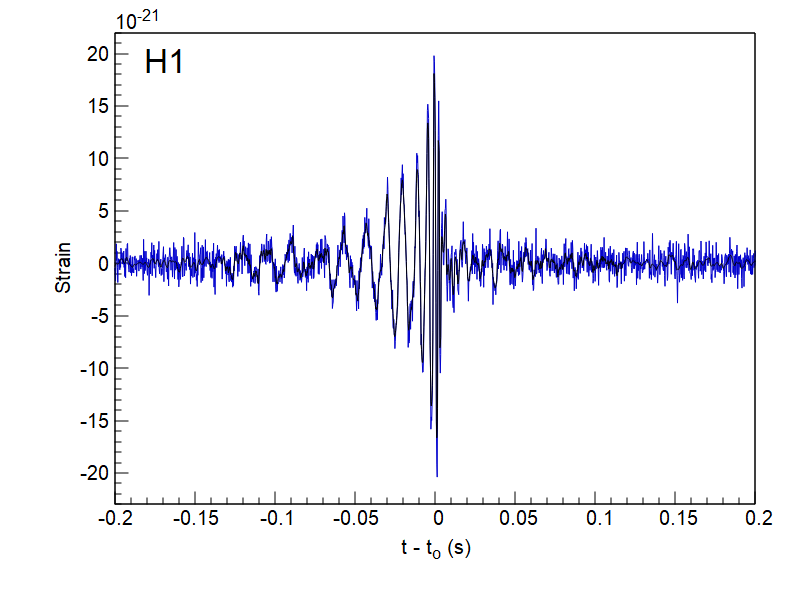
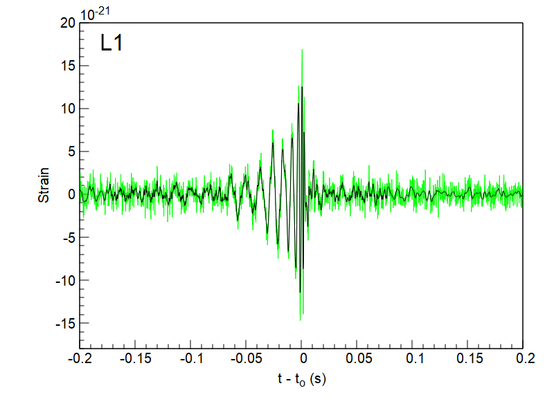
Figure 1: Comparison between the GW150914 whitened and denoised strains for both H1 (left panel) and L1 (right panel). The denoised strains (black lines) are obtained after the application of the rROF method to the whitened strain data, using the optimal set of parameter values of Table 1. Whitened strains are shown in blue (H1) and in green (L1).

Data analysis with the cWB pipeline starts first with the data-conditioning step. This is done utilizing a regression algorithm [37] that identifies and removes persistent lines and noise artefacts. Afterwards, the data is whitened and converted to the TF domain using the WDM wavelet transformation [38]. This analysis is repeated several times at several frequency resolutions to obtain good TF coverage for a broad range of signal morphologies. Candidate events can be identified as a cluster of TF data samples with power above the baseline detector noise. In the final step, the pipeline reconstructs the signal waveforms, the wave polarization and the source sky localization using a constrained maximum likelihood analysis over the GW detector network [24, 23].

The cWB pipeline is written in C++ and is used in combination with several ROOT macros. The main functions of the pipeline manage the external ROOT macros to use them for specific tasks to perform the cWB analysis. This structure allows the possibility of adding external routines of any kind, called plugins, for any specific purpose that can be combined with the default analysis procedure of the pipeline. The implementation of the rROF algorithm in the cWB pipeline, both using its original design as well as the iterative regularization extension, has been developed as plugins. A first plugin was built for the single-step rROF method. This routine operates over the data stream after the whitening step, which is performed by the pipeline itself. The integration at this point of the analysis procedure ensures that the application of the rROF algorithm is independent of the frequency range of the data, as well as of the parameters intrinsic to the algorithm. A second plugin has also been developed for the iterative rROF algorithm. When used, this second plugin operates in replacement of the rROF plugin in the cWB pipeline under the same conditions.

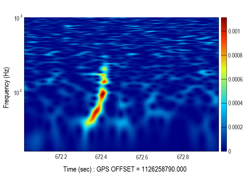
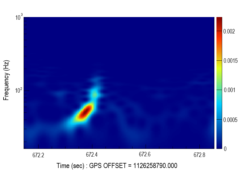
Figure 2: cWB spectrograms for the GW150914 waveform. The left spectrograms are cWB-only results while the right ones correspond to the combined cWB+rROF results. Data on the top panels are for L1 while those on the bottom panels are for H1.

IV Results

To test the implementation and performance of the rROF denoising method in the cWB pipeline we employ real GW strain data freely accessible through the Gravitational Wave Open Science Center [39]. The signals we select are two O1 detections, GW150914 [5] and GW151226 [6], the BNS merger event in O2 GW170817 [8], and the intermediate-mass black hole event in O3 GW190521 [40]. Most of the following discussion is focused in GW150914 which we take as an illustrative example to assess the method. The evaluation procedure is as follows: first, we determine the optimal parameter values of the original rROF method for the GW150914 event; next, we perform the data analysis with the cWB pipeline equipped with the rROF denoising method; finally, we compare these results with those the cWB pipeline yields when the rROF denoising substep is not operational. The same approach is then repeated for the iterative rROF algorithm.

IV.1 Selection of rROF parameters for GW150914

Since GW150914 was observed by the two Advanced LIGO interferometers, two sets of rROF parameter values need to be determined, one for each detector. With this purpose, we use the BBH waveforms computed by the cWB pipeline as the reference template to tune the parameters required by the rROF method. Table 1 reports the optimal set of parameter values we obtain for GW150914.

Table 1: Optimal parameter values of the GW150914 event obtained with the rROF algorithm. Results of the WS are also shown in the last column.

Detector	$h$	$\beta$	$\lambda$	tol	$N$	WS
L1	0.3	0.5	0.02	0.2	1024	30
H1	0.1	0.5	0.01	0.2	512	31

The strain data is extracted from the cWB pipeline after data-conditioning and whitening. Figure 1 shows the denoised waveforms for GW150914 with the optimal parameter values listed in Table 1. The black lines represent the denoised data from the whitened strains for both H1 (blue line, left panel) and L1 (green line, right panel). As this figure shows, the morphology of the reference template waveform is properly preserved after the denoising. The evaluation of the rROF method is measured with the WS estimator. We find that about 70% of the original noise contained in the signal is subtracted in the case of L1 data (69% for H1 data) while the waveform is preserved quite accurately.

We note that the strain data shown in Figure 1 is obtained directly from the cWB pipeline right after the whitening process, the last step of the data-conditioning stage. This stage includes all quality controls, vetoes and removal of potential glitches. As a result, the waveforms show some modifications with respect to the original GW150914 raw-strain data plotted in [5]. Our focus in Figure 1 is to highlight the difference in the whitened strain when the denoising rROF step is applied or otherwise.

IV.2 Combined analysis of GW150914

We now reanalyse GW150914 with the active implementation of the rROF method in the cWB pipeline, using the optimal parameters of Table 1. The cWB data analysis reported a successful identification and wave reconstruction of the GW150914 event for both H1 and L1. The original (cWB only) and the reconstructed (cWB+rROF) spectrograms for the two interferometers are shown in Figure 2. The left panels display the original cWB results and the right panels the results obtained with the addition of the rROF step (L1 is shown on the top and H1 on the bottom). The overall reduction of the noise contained in the data is visible in the right plots, providing a clearer view of the GW150914 chirp signal. However, the average amplitude of the event is reduced as well. This is to be expected since the detected signal is a combination of the actual gravitational waveform and some amount of noise. Further inspection of the spectrograms reveals that the rROF step also causes the high-frequency component of the signal (the ringdown part above 150 Hz approximately) not to display as prominently in the denoised data as it does in the original cWB spectrogram. The visual comparison of the spectrograms shows, indeed, that a portion of the signal at the higher frequencies is missing in the combined denoised result.

To further quantify the comparison we analyse the output of some of the statistical parameters reported by the cWB pipeline. A selection is shown in Table 2 including the SNR, the effective correlated amplitude $\rho$, the correlation coefficient cc, and the network energy disbalance ED. The effective correlated amplitude is obtained from the SNR according to (assuming a network correlation near to one):

$$\rho=\sqrt{\frac{\Sigma_{i}{\rm SNR}_{i}}{2N_{\rm IFO}}},$$ (11)

where $N_{\rm IFO}$ is the number of interferometers active during an event and SNR_i is the signal to noise ratio of the individual interferometers. We observe that the values of both the SNR and $\rho$ are significantly reduced when the rROF denoising step is active. This result is unexpected since a reduction of the noise present in the data should produce an increase of both quantities. On the other hand, the coherence coefficient $cc$ increases by $3.2\%$, from 0.93 to 0.96, when the rROF step is active. Hence, this coefficient behaves as one would expect in the case of noise reduction from the data.

Table 2: Parameters reported by the cWB pipeline for the analysis of the GW150914 event, with and without the activation of the rROF algorithm.

	SNR	$\rho$(L1)	$\rho$(H1)	cc	ED
W/o rROF	25.2	16.7	16.0	0.93	-0.01
With rROF	15.5	9.8	9.5	0.96	-0.05

IV.3 Analysis of GW150914 with iterative rROF

From the results we have just described it becomes clear that the application of the single-step rROF method does not improve the results of the standalone cWB pipeline, at least for the case of the GW150914 waveform. The single-step denoising subtracts a significant fraction of the signal at the higher frequencies.

Here we reanalyze this event by combining the cWB pipeline with the iterative rROF algorithm as the denoising step, as described in Section II.3. This method is designed to compensate for the deficiencies of the single-step denoising, which occurs when there is significant data loss. The values of the parameters of the method used in this case are shown in the first row of Table 3. These values are determined heuristically by increasing the values regarded as optimal for the single-step algorithm, determined in Section IV.1. We note that we do not need to perform a second parametrization as the iterative method is based on the successive application of the single-step algorithm with sub-optimal parameter values, combined with the use of a data quality check after each step until the stopping condition is reached. This procedure still uses the same low-pass filtering rROF algorithm implemented in the cWB+rROF combined analysis. While the algorithm still behaves effectively as a low-pass filter the fact of adding back the residual to the initial data several times improves significantly the quality of the denoising in the high-frequency part of the signal.

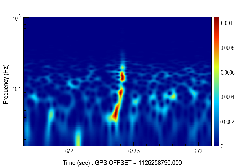
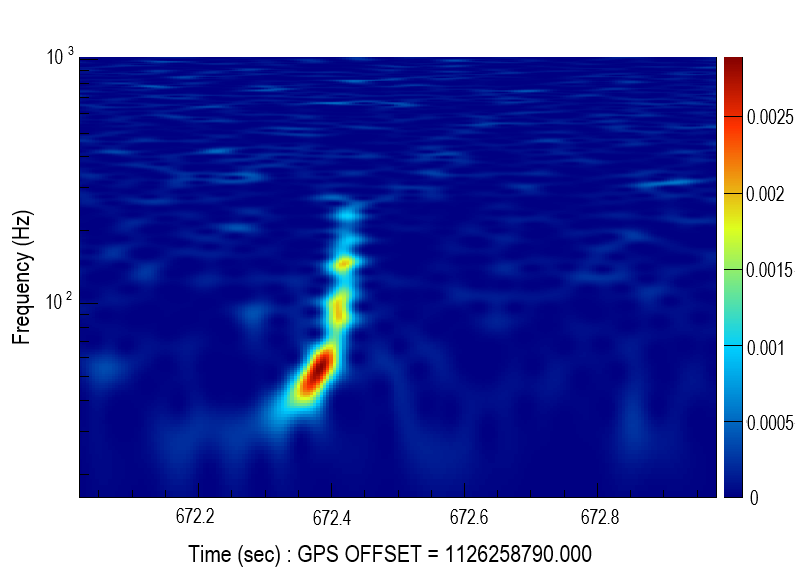
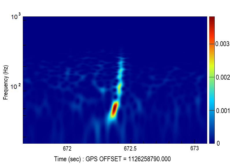
Figure 3: cWB spectrograms for the GW150914 waveform. The left spectrograms are cWB-only results while the right ones correspond to the combined cWB and iterative rROF results. Data on the top panels are for L1 while those on the bottom panels are for H1.

Table 3: Parameter values of the iterative rROF algorithm for the GW events considered in this work.

GW event	$h$	$\beta$	$\lambda$	tol	$N$
GW150914	1	1	0.1	0.2	1024
GW151226	1	1	0.2	0.2	1024
GW170817	1	1	1.0	0.001	1024
GW190521	1	1	0.1	0.2	1024

The cWB pipeline reports once again a successful identification and waveform reconstruction of the GW150914 event. Figure 3 displays the new spectrograms obtained from the cWB pipeline for L1 (top panels) and H1 (bottom panels). The left column shows the original cWB spectrograms without any denoising step active (as in the left panels of Fig. 2) and the right column the corresponding spectrograms obtained with the combined cWB and iterative rROF algorithm.

As for the case of the single-step rROF method, the iterative rROF algorithm also yields a visible overall reduction of noise which provides a somewhat clearer track of the chirp, specially at frequencies higher than $\approx 150$ Hz. The most notable difference with respect to the single-step rROF method is that the iterative rROF algorithm succeeds in keeping the high-frequency part of the signal intact, showing no data loss above $\approx 150$ Hz (compare the right panels of Fig. 2 and Fig 3). Therefore, when combining the cWB pipeline with the iterative rROF algorithm the complete ringdown part of the GW150914 signal remains intact and clearly visible. We also notice that the spectrograms of the denoised signals are extremely clean at high frequencies (displaying a uniformly dark blue) as was also the case when using the single-step rROF method. For the latter, that is an indication that the rROF algorithm behaves as a low-pass filter. With iterative regularization this is still the case since the rROF algorithm is used at every iteration. However, by adding the residual back to the signal the rROF algorithm behaves as a low-pass filter just for noise, thus keeping intact the signal contained in the data.

When inspecting the numerical values of the statistical parameters computed by the cWB pipeline when used in combination with the iterative rROF algorithm, we pay special attention to the reported SNR as our main indicator of a successful denoising. As shown in the first row of Table 4, the SNR of the GW150914 event increases from 25.2 to 27.1, an enhancement of 7.5% with respect to the original cWB measurement. We thus conclude that the results obtained with the iterative denoising for our selected test case, GW150914, are worth considering.

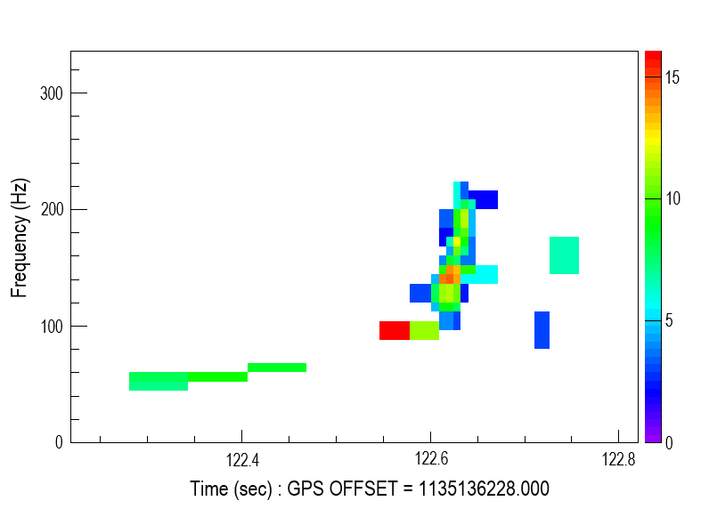
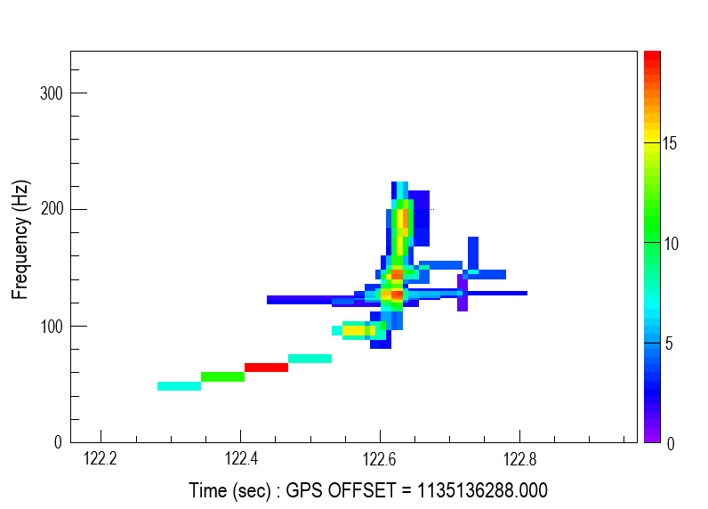
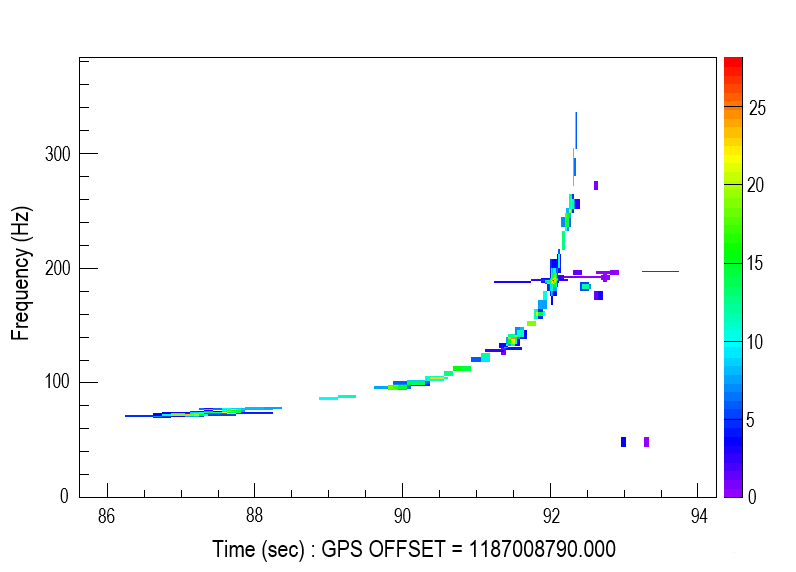
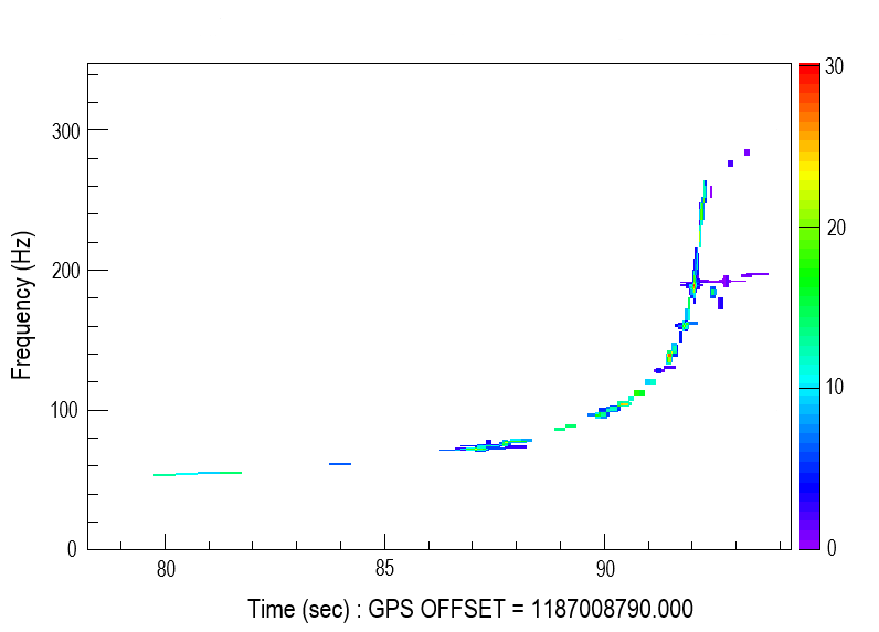
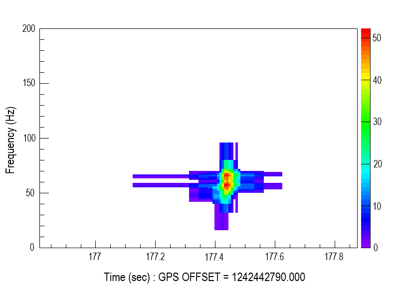
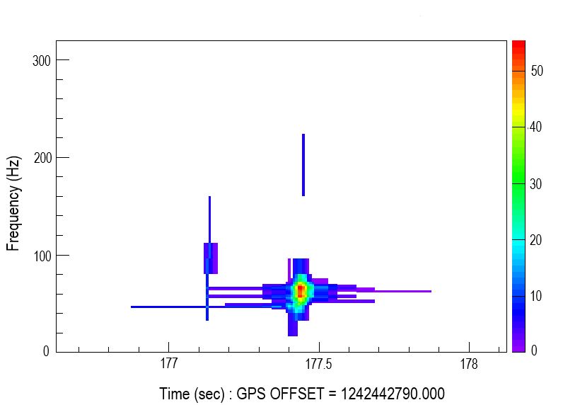
Figure 4: Likelihoods computed by the cWB pipeline for GW events GW151226 (top), GW170817 (centre), and GW190521 (bottom). In the results displayed in the left column the rROF method is not active. The right column shows the corresponding likelihoods when cWB is combined with the iterative rROF algorithm.

IV.4 Additional GW events

To complete the assessment of the rROF method as a denoising plugin of the cWB pipeline we extend our investigation to additional GW events. We aim to prove that the denoising method can provide positive results with any signal type regardless of the nature of the noise contained in the data. To do this we select events GW151226, a BBH merger signal from observing run O1 [6], GW170817, the BNS merger event detected in O2 [8], and GW190521, an intermediate-mass black hole signal observed in O3 [40]. The corresponding SNR values computed by cWB are reported in Table 4.

We begin by using the cWB pipeline in combination with the single-step rROF algorithm. For none of the three events the pipeline is able to report a detection. Our conclusion is that in all three cases the subtraction of signal during the denoising step is more severe than in the case of GW150914, despite the fact that we used the optimal parameter values as determined for each event separately. By removing too much signal from the data the cWB pipeline is unable to achieve an identification. Our hypothesis is that it might be related to the low-frequency filtering nature of the rROF algorithm, which does not perform appropriately for the low SNR event GW151226 nor for the high-frequency signal GW170817. To obtain a conclusive statement would require a deeper analysis of the data subtracted by the rROF denoising.

However, the combined application of cWB and the iterative rROF method to the additional GW events yields entirely satisfactory results. Using the specific values of the iterative rROF method parameters indicated in Table 3 we find that all three signals are identified by the cWB pipeline, the analysis software is able to reconstruct all events and in all cases it reports an enhancement in the waveform SNR. Table 4 summarizes the SNR values obtained for the four GW events analysed in this work. The specific SNR increments are 7.5% (GW150914), 17.6% (GW151226), 1.1% (GW170817), and 14.2% (GW190521).

Figure 4 displays the likelihood computed by cWB for each event: GW151226 in the top row, GW170817 in the central row, and GW190521 at the bottom. The left column shows the likelihood for each event without the use of a rROF denoising step, while the right column displays the corresponding likelihood with the iterative rROF algorithm active. This figure demonstrates that for all GW events considered, the waveforms are identified and properly reconstructed by the cWB pipeline. The iterative rROF algorithm does not introduce any kind of data loss in any part of the spectrograms, in particular in the high-frequency region.

Finally, we come back to the issue of the parameter values used by the iterative regularization, reported in Table 3. The methodology indicates that values higher than the optimal ones should be used. For all signals considered the parameter selection has been made aiming to find an acceptable denoising result, taking advantage of the flexibility that the iterative regularization offers. Moreover, a completely operational denoising method should be able to successfully operate on any kind of data, without any prior knowledge about the signal. In this regard, the possibility of using free parameters independent of the kind of noise or signal is in our interest. This is indeed an attractive additional possibility iterative regularization offers.

Table 4: Values of the SNR computed by cWB for the GW events considered in this work. SNR_a corresponds to the purely cWB value (no rROF step) while SNR_b is the SNR obtained using cWB in combination with the iterative rROF method.

Event	Type	Run	SNRa	SNRb
GW150914	BBH	O1	25.2	27.1
GW151226	BBH	O1	11.9	14.0
GW170817	BNS	O2	26.8	27.1
GW190521	IMBH	O3	14.7	16.8

V Conclusions

The rate of detections of GW signals by the Advanced LIGO-Virgo-KAGRA interferometer network is dramatically increasing with every detector update [9]. The data collected are largely dominated by instrumental noise which renders data denoising and signal reconstruction truly important efforts. In such context, the denoising of GW signals based on $L_{1}$-norm minimization approaches shows strong potential, as evidenced by the results reported in [18, 20, 21, 22]. Those studies have shown that the regularized Rudin-Osher-Fatemi method [19] is suitable to denoise GW signals embedded either in additive Gaussian noise [18] or in actual detector noise [20], irrespective of the signal morphology, data conditioning, or whitening.

In this paper, we have extended those studies by discussing the implementation and calibration of the rROF method in an existing GW data-analysis pipeline, with the mid-term goal of having it operational in upcoming LVK data-taking runs. We have selected the cWB pipeline, designed for coherent searches of unmodelled burst sources [23, 24] and we have implemented the rROF method as a plug-in within the flowchart of the pipeline. Additionally, building on a proposal laid out in [18] we have also implemented an iterative regularization approach (as a second plug-in) using the single-step rROF algorithm as the base denosing method for each iteration. The combined cWB+rROF approach has initially been tested using actual noisy data from the GW150914 event. The comparison between the results of the cWB pipeline with and without the rROF denoising substep has revealed some limitations of the single-step rROF method. Our implementation of the algorithm has led, in particular, to a significant elimination of the high-frequency component of the signal (along with the anticipated noise removal). The remedy to this drawback has been found in the iterative rROF algorithm, an approach proposed as an improvement over the original model, especially formulated to compensate for the signal removal sometimes present in a single-step rROF method. The assessment of the iterative rROF algorithm with the GW150914 waveform has led to satisfactory results. We have found that a notable amount of noise can be removed while at the same time the entire signal morphology is unaffected at all frequencies, yielding an increment in the cWB analysis indicators, most importantly the SNR.

Our analysis has been completed with three additional GW events, spanning representative CBC morphologies and detector noise, namely a second BBH merger from O1, GW151226, the BNS merger event from O2 GW170817, and the intermediate-mass black hole event from O3 GW190521. For all of these events we have also observed that the iterative version of the rROF algorithm implemented in the cWB pipeline leads to an effectual reduction of the noise without affecting the signals, thus yielding enhanced SNR values. For GW170817 the SNR increment is a modest 1.1% while for GW151226 and GW190521 is 17.6% and 14.2%, respectively.

As a near-term goal we plan to perform offline analysis of the complete O1-O3 data with the combined cWB + iterative rROF pipeline. By doing so we will reevaluate the detectability capabilities of the pipeline for existing triggers and the inference of the source properties, as well as investigate whether the improved quality of the data may lead to unveil potential new triggers on the available data. In addition, we also plan to implement and deploy the iterative rROF method in the low-latency version of the cWB pipeline for O4 and O5. The experience to be gained with the O1-O3 searches should pave the way to the eventual application of the denosing technique discussed in this paper to the upcoming observational campaigns of the LIGO-Virgo-KAGRA detector network.