Transformer Quality in Linear Time

Abstract

We revisit the design choices in Transformers, and propose methods to address their weaknesses in handling long sequences. First, we propose a simple layer named gated attention unit, which allows the use of a weaker single-head attention with minimal quality loss. We then propose a linear approximation method complementary to this new layer, which is accelerator-friendly and highly competitive in quality. The resulting model, named FLASH , matches the perplexity of improved Transformers over both short (512) and long (8K) context lengths, achieving training speedups of up to 4.9$\times$ on Wiki-40B and 12.1$\times$ on PG-19 for auto-regressive language modeling, and 4.8$\times$ on C4 for masked language modeling.

1 Introduction

Transformers (Vaswani et al., 2017) have become the new engine of state-of-the-art deep learning systems, leading to many recent breakthroughs in language (Devlin et al., 2018; Brown et al., 2020) and vision (Dosovitskiy et al., 2020). Although they have been growing in model size, most Transformers are still limited to short context size due to their quadratic complexity over the input length. This limitation prevents Transformer models from processing long-term information, a critical property for many applications.

Many techniques have been proposed to speedup Transformers over extended context via more efficient attention mechanisms (Child et al., 2019; Dai et al., 2019; Rae et al., 2019; Choromanski et al., 2020; Wang et al., 2020; Katharopoulos et al., 2020; Beltagy et al., 2020; Zaheer et al., 2020; Kitaev et al., 2020; Roy et al., 2021; Jaegle et al., 2021). Despite the linear theoretical complexity for some of those methods, vanilla Transformers still remain as the dominant choice in state-of-the-art systems. Here we examine this issue from a practical perspective, and find existing efficient attention methods suffer from at least one of the following drawbacks:

	Speedup
Length	over TFM	over TFM++
512	1.8$\times$	1.2$\times$
1024	9.0$\times$	1.3$\times$
2048	8.9$\times$	1.6$\times$
4096	13.1$\times$	2.7$\times$
8192	25.6$\times$	4.9$\times$

Figure 1: TPU-v4 training speedup of FLASH relative to the vanilla Transformer (TFM) and an augmented Transformer (TFM++) for auto-regressive language modeling on Wiki-40B — All models are comparable in size at around 110M and trained for 125K steps with 2¹⁸ tokens per batch.

⬇

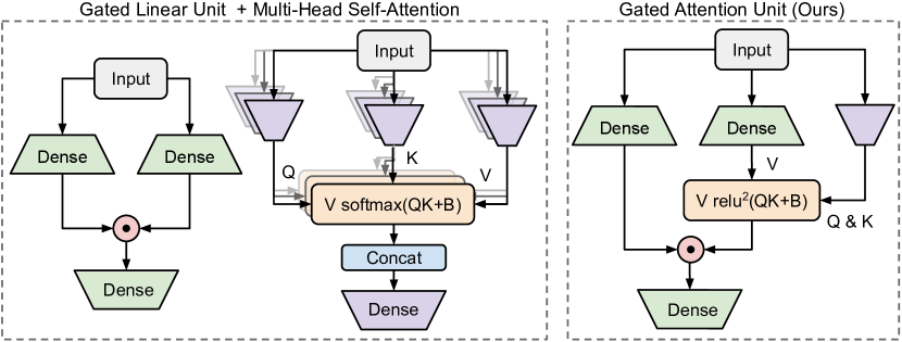
def scale_offset(x):

gamma = var(x.shape[-1:])

beta = var(x.shape[-1:])

return x * gamma + beta

def attn(x, v, s=128):

z = dense(x, s)

q, k = scale_offset(z), scale_offset(z)

qk = tf.einsum('bns,bms$\rightarrow$bnm', q, k)

a = relu(qk + rel_pos_bias(q, k)) ** 2

return tf.einsum('bnm,bme$\rightarrow$bne', a, v)

def gated_attn_unit(x, d=768, e=1536):

shortcut, x = x, norm(x)

u, v = dense(x, e), dense(x, e)

x = u * attn(x, v)

return dense(x, d) + shortcut

Figure 2: (a) An augmented Transformer layer which consists of two blocks: Gated Linear Unit (GLU) and Multi-Head Self-Attention (MHSA), (b) Our proposed Gated Attention Unit (GAU), (c) Pseudocode for Gated Attention Unit. Skip connection and input normalization over the residual branch are omitted in (a), (b) for brevity.

• Inferior Quality. Our studies reveal that vanilla Transformers, when augmented with several simple tweaks, can be much stronger than the common baselines used in the literature (see Transformer vs. Transformer++ in Figure 1). Existing efficient attention methods often incur significant quality drop compared to augmented Transformers, and this drop outweighs their efficiency benefits.

• Overhead in Practice. As efficient attention methods often complicate Transformer layers and require extensive memory re-formatting operations, there can be a nontrivial gap between their theoretical complexity and empirical speed on accelerators such as GPUs or TPUs.

• Inefficient Auto-regressive Training. Most attention linearization techniques enjoy fast decoding during inference, but can be extremely slow to train on auto-regressive tasks such as language modeling. This is primarily due to their RNN-style sequential state updates over a large number of steps, making it infeasible to fully leverage the strength of modern accelerators during training.

We address the above issues by developing a new model family that, for the first time, not only achieves parity with fully augmented Transformers in quality, but also truly enjoys linear scalability over the context size on modern accelerators. Unlike existing efficient attention methods which directly aim to approximate the multi-head self-attention (MHSA) in Transformers, we start with a new layer design which naturally enables higher-quality approximation. Specifically, our model, named FLASH, is developed in two steps:

First, we propose a new layer that is more desirable for effective approximation. We introduce a gating mechanism to alleviate the burden of self-attention, resulting in the Gated Attention Unit (GAU) in Figure 2. As compared to Transformer layers, each GAU layer is cheaper, and more importantly, its quality relies less on the precision of attention. In fact, GAU with a small single-head, softmax-free attention is as performant as Transformers. While GAU still suffers from quadratic complexity over the context size, it weakens the role of attention hence allows us to carry out approximation later with minimal quality loss.

We then propose an efficient method to approximate the quadratic attention in GAU, leading to a layer variant with linear complexity over the context size. The key idea is to first group tokens into chunks, then using precise quadratic attention within a chunk and fast linear attention across chunks, as illustrated in Figure 4. We further describe how an accelerator-efficient implementation can be naturally derived from this formulation, achieving linear scalability in practice with only a few lines of code change.

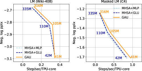
	Layer Type	# of Layers	$d$
	MHSA+MLP	8+8	512
		12+12	768
		24+24	1024
	MHSA+GLU	8+8	512
		12+12	768
		24+24	1024
	GAU	15	512
		22	768
		46	1024

Figure 3: GAU vs. Transformers for auto-regressive and masked language modeling on short context length (512).

We conduct extensive experiments to demonstrate the efficacy of FLASH over a variety of tasks (masked and auto-regressive language modeling), datasets (C4, Wiki-40B, PG-19) and model scales (110M to 500M). Remarkably, FLASH is competitive with fully-augmented Transformers (Transformer++) in quality across a wide range of context sizes of practical interest (512–8K), while achieving linear scalability on modern hardware accelerators. For example, with comparable quality, FLASH achieves a speedup of 1.2$\times$–4.9$\times$ for language modeling on Wiki-40B and a speedup of 1.0$\times$–4.8$\times$ for masked language modeling on C4 over Transformer++. As we further scale up to PG-19 (Rae et al., 2019), FLASH reduces the training cost of Transformer++ by up to 12.1$\times$ and achieves significant gain in quality.

2 Gated Attention Unit

Here we present Gated Attention Unit (GAU), a simpler yet more performant layer than Transformers. While GAU still has quadratic complexity over the context length, it is more desirable for the approximation method to be presented in Section 3. We start with introducing related layers:

Vanilla MLP.

Let $X\in\mathbb{R}^{T\times d}$ be the representations over $T$ tokens. The output for Transformer’s MLP can be formulated as $O=\phi(XW_{u})W_{o}$ where $W_{u}\in\mathbb{R}^{d\times e}$, $W_{o}\in\mathbb{R}^{e\times d}$. Here $d$ denotes the model size, $e$ denotes the expanded intermediate size, and $\phi$ is an element-wise activation function.

Gated Linear Unit (GLU).

This is an improved MLP augmented with gating (Dauphin et al., 2017). GLU has been proven effective in many cases (Shazeer, 2020; Narang et al., 2021) and is used in state-of-the-art Transformer language models (Du et al., 2021; Thoppilan et al., 2022).

$$U =\phi_{u}(XW_{u}),\quad V=\phi_{v}(XW_{v}) \in\mathbb{R}^{T\times e}$$ (1)

$$O =(U\odot V)W_{o} \in\mathbb{R}^{T\times d}$$ (2)

where $\odot$ stands for element-wise multiplication. In GLU, each representation $u_{i}$ is gated by another representation $v_{i}$ associated with the same token.

Gated Attention Unit (GAU).

The key idea is to formulate attention and GLU as a unified layer and to share their computation as much as possible (Figure 2). This not only results in higher param/compute efficiency, but also naturally enables a powerful attentive gating mechanism. Specifically, GAU generalizes Eq. (2) in GLU as follows:

$$O =(U\odot\hat{V})W_{o}\quad\text{where}\quad\hat{V}=AV$$ (3)

where $A\in\mathbb{R}^{T\times T}$ contains token-token attention weights. Unlike GLU which always uses $v_{i}$ to gate $u_{i}$ (both associated with the same token), our GAU replaces $v_{i}$ with a potentially more relevant representation $\hat{v}_{i}=\sum_{j}a_{ij}v_{j}$ “retrieved” from all available tokens using attention. The above will reduce to GLU when $A$ is an identity matrix.

Consistent with the findings in Liu et al. (2021), the presence of gating allows the use of a much simpler/weaker attention mechanism than MHSA without quality loss:

$$Z =\phi_{z}(XW_{z}) \in\mathbb{R}^{T\times s}$$ (4)

$$A =\mathrm{relu}^{2}\left(\mathcal{Q}(Z)\mathcal{K}(Z)^{\top}+b\right) \in\mathbb{R}^{T\times T}$$ (5)

Modifications	PPLX (LM/MLM)	Params (M)
original GAU	16.78 / 4.23	105
relu2 $\xrightarrow{}$ softmax	17.04 / 4.31	105
single-head $\xrightarrow{}$ multi-head	17.76 / 4.48	105
no gating	17.45 / 4.58	131

Table 1: Impact of various modifications on GAU.

Modifications	PPLX (LM/MLM)	Params (M)
original MHSA	16.87 / 4.35	110
softmax $\xrightarrow{}$ relu2	17.15 / 4.77	110
multi-head $\xrightarrow{}$ single-head	17.89 / 4.73	110
add gating	17.25 / 4.43	106

Table 2: Impact of various modifications on MHSA.

where $Z$ is a shared representation ($s\ll d$), $\mathcal{Q}$ and $\mathcal{K}$ are two cheap transformations that apply per-dim scalars and offsets to $Z$ (similar to the learnable variables in LayerNorms), and $b$ is the relative position bias. We also find the softmax in MHSA can be simplified as a regular activation function in the case of GAU. The GAU layer and its pseudocode are illustrated in Figure 2.

Unlike Transformer’s MHSA which comes with $4d^{2}$ parameters, GAU’s attention introduces only a single small dense matrix $W_{z}$ with $ds$ parameters on top of GLU (scalars and offsets in $\mathcal{Q}$ and $\mathcal{K}$ are negligible). By setting $e=2d$ for GAU, this compact design allows us to replace each Transformer block (MLP/GLU + MHSA) with two GAUs while retaining similar model size and training speed.

GAU vs. Transformers.

Figure 3 shows that GAUs are competitive with Transformers (MSHA + MLP/GLU) on TPUs across different models sizes. Note these experiments are conducted over a relatively short context size (512). We will see later in Section 4 that GAUs are in fact even more performant when the context length is longer, thanks to their reduced capacity in attention.

Layer Ablations.

In Table 1 & 2 we show that both GAUs and Transformers are locally optimal on their own.

3 Fast Linear Attention with GAU

There are two observations from Section 2 that motivate us to extend GAU to modeling long sequences:

• First, the gating mechanism in GAU allows the use of a weaker (single-headed, softmax-free) attention without quality loss. If we further adapt this intuition into modeling long sequences with attention, GAU could also boost the effectiveness of approximate (weak) attention mechanisms such as local, sparse and linearized attention.

• In addition, the number of attention modules is naturally doubled with GAU — recall MLP+MHSA$\approx$2$\times$GAU in terms of cost (Section 2). Since approximate attention usually requires more layers to capture full dependency (Dai et al., 2019; Child et al., 2019), this property also makes GAU more appealing in handling long sequences.

With this intuition in mind, we start by reviewing some related work on modeling long sequences with attention, and then show how we enable GAU to achieve Transformer-level quality in linear time on long sequences.

3.1 Existing Linear-Complexity Variants

Partial Attention.

A popular class of methods tries to approximate the full attention matrix with different partial/sparse patterns, including local window (Dai et al., 2019; Rae et al., 2019), local+sparse (Child et al., 2019; Li et al., 2019; Beltagy et al., 2020; Zaheer et al., 2020), axial (Ho et al., 2019; Huang et al., 2019), learnable patterns through hashing (Kitaev et al., 2020) or clustering (Roy et al., 2021). Though not as effective as full attention, these variants are usually able to enjoy quality gains from scaling to longer sequences. However, the key problem with this class of methods is that they involve extensive irregular or regular memory re-formatting operations such as gather, scatter, slice and concatenation, which are not friendly to modern accelerators of massive parallelism, particularly specialized ASICs like TPU. As a result, their practical benefits (speed and RAM efficiency), if any, largely depend on the choice of accelerator and usually fall behind the theoretical analysis. Hence, in this work, we deliberately minimize the number of memory re-formatting operations in our model.

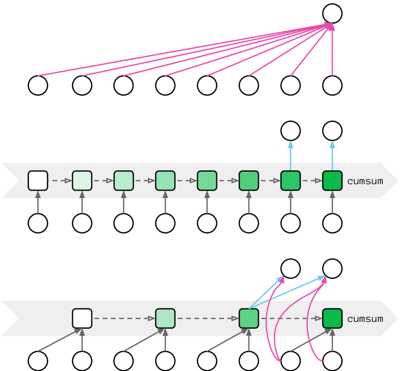
Figure 4: (top) Quadratic attention, (mid) Linear attention, (bottom) Proposed mixed chunk attention with a chunk size ($C$) of 2 ($C$ is always greater than or equal to 128 in our experiments). Our method significantly reduces the compute in quadratic attention (red links), while requiring substantially less RNN-style steps (green squares) in conventional linear attention.

Linear Attention.

Alternatively, another popular line of research linearizes the attention computation by decomposing the attention matrix and then re-arranging the order of matrix multiplications (Choromanski et al., 2020; Wang et al., 2020; Katharopoulos et al., 2020; Peng et al., 2021). Schematically, the linear attention can be expressed as

$$\hat{V}_{\text{lin}}=Q\underbrace{\left(K^{\top}V\right)}_{\mathbb{R}^{d\times d}}\ \xrightarrow{\text{approx}}\ \hat{V}_{\text{quad}}=\mathrm{Softmax}\underbrace{\left(QK^{\top}\right)}_{\mathbb{R}^{T\times T}}V$$

where $Q,K,V\in\mathbb{R}^{T\times d}$ are the query, key and value representations, respectively. Re-arranging the computation reduces the complexity w.r.t $T$ from quadratic to linear.

Another desirable property of linear attention is its constant computation and memory for each auto-regressive decoding step at inference time. To see that, define $M_{t}=K_{:t}^{\top}V_{:t}$ and notice that the computation of $M_{t}$ can be fully incremental:

$$M_{t}=M_{t-1}+K_{t}V_{t}^{\top}$$ (6)

This means we only need to maintain a cache with constant $\mathcal{O}(d^{2})$ memory and whenever a new input arrives at time stamp $t$, only constant $\mathcal{O}(d^{2})$ computation is required to accumulate $K_{t}V_{t}^{\top}$ into $M_{t-1}$ and get $M_{t}$. On the contrary, full quadratic attention requires linear $\mathcal{O}(Td)$ computation and memory for each decoding step, as each new input has to attend to all the previous steps.

However, on the other hand, re-arranging the computation in linear attention leads to a severe inefficiency during auto-regressive training. As shown in Fig. 4 (mid), due to the causal constraint for auto-regressive training, the query vector at each time step $Q_{t}$ corresponds to a different cache value $M_{t}=K_{:t}^{\top}V_{:t}$. This requires the model to compute and cache $T$ different values $\{M_{t}\}_{t=1}^{T}$ instead of only one value $K^{\top}V$ in the non-autoregressive case. In theory, the sequence $\{M_{t}\}_{t=1}^{T}$ can be obtained in $\mathcal{O}(Td^{2})$ by first computing $\{K_{t}V_{t}^{\top}\}_{t=1}^{T}$ and then performing a large cumulative sum (cumsum) over $T$ tokens. But in practice, the cumsum introduces an RNN-style sequential dependency of $T$ steps, where an $\mathcal{O}(d^{2})$ state needs to be processed each step. The sequential dependency not only limits the degree of parallelism, but more importantly requires $T$ memory access in the loop, which usually costs much more time than computing the element-wise addition on modern accelerators. As a result, there exists a considerable gap between the theoretical complexity and actual running time. In practice, we find that directly computing the full quadratic attention matrix is even faster than the re-arranged (linearized) version on both TPUs (Figure 6(a)) and GPUs (Appendix C.1).

3.2 Our Method: Mixed Chunk Attention

Based on the strengths and weaknesses of existing linear-complexity attentions, we propose mixed chunk attention, which merges the benefits from both partial attention and linear attention. The high-level idea is illustrated in Figure 4. Below we reformulate GAU to incorporate this idea.

Preparation.

The input sequence is first chunked into $G$ non-overlapping chunks of size $C$, i.e. $[T]\to[T/C\times C]$. Then, $U_{g}\in\mathbb{R}^{C\times e}$, $V_{g}\in\mathbb{R}^{C\times e}$ and $Z_{g}\in\mathbb{R}^{C\times s}$ are produced for each chunk $g$ following the GAU formulation in Eq. (1) and Eq. (4). Next, four types of attention heads $Q_{g}^{\text{quad}}$, $K_{g}^{\text{quad}}$, $Q_{g}^{\text{lin}}$, $K_{g}^{\text{lin}}$ are produced from $Z_{g}$ by applying per-dim scaling and offset (this is very cheap).

We will describe how GAU’s attention can be efficiently approximated using a local attention plus a global attention. Note all the major tensors $U_{g}$, $V_{g}$ and $Z_{g}$ are shared between the two components. The only additional parameters introduced over the original GAU are the per-dim scalars and offsets for generating $Q_{g}^{\text{lin}}$ and $K_{g}^{\text{lin}}$ (4$\times s$ parameters).

Local Attention per Chunk.

First, a local quadratic attention is independently applied to each chunk of length $C$ to produce part of the pre-gating state:

$$\hat{V}_{g}^{\text{quad}}=\mathrm{relu}^{2}\Big{(}Q_{g}^{\text{quad}}{K_{g}^{\text{quad}}}^{\top}+b\Big{)}V_{g}.$$

The complexity of this part is $\mathcal{O}(G\times C^{2}\times d)=\mathcal{O}(TCd)$, which is linear in $T$ given that $C$ remains constant.

Global Attention across Chunks.

In addition, a global linear attention mechanism is employed to capture long-range interaction across chunks

Non-Causal: $$\hat{V}_{g}^{\text{lin}} =Q_{g}^{\text{lin}}\bigg{(}\sum_{h=1}^{G}{K_{h}^{\text{lin}}}^{\top}V_{h}\bigg{)},$$ (7)

Causal: $$\hat{V}_{g}^{\text{lin}} =Q_{g}^{\text{lin}}\bigg{(}\sum_{h=1}^{g-1}{K_{h}^{\text{lin}}}^{\top}V_{h}\bigg{)}.$$ (8)

Note the summations in Eq. (7) and Eq. (8) are performed at the chunk level. For the causal (auto-regressive) case, this reduces the number of elements in the cumsum in token-level linear attention by a factor of $C$ (a typical $C$ is 256 in our experiments), leading to a significant training speedup.

Finally, $\hat{V}_{g}^{\text{quad}}$ and $\hat{V}_{g}^{\text{lin}}$ are added together, followed by gating and a post-attention projection analogous to Eq. (3):

$$O_{g}=\left[U_{g}\odot\left(\hat{V}_{g}^{\text{quad}}+\hat{V}_{g}^{\text{lin}}\right)\right]W_{o}.$$

The mixed chunk attention is simple to implement and the corresponding pseudocode is given in Code 1.

⬇

def _global_linear_attn(q, k, v, causal):

if causal:

kv = tf.einsum('bgcs,bgce$\rightarrow$bgse', k, v)

kv = tf.cumsum(kv, axis=1, exclusive=True)

return tf.einsum('bgcs,bgse$\rightarrow$bgce', q, kv)

else:

kv = tf.einsum('bgcs,bgce$\rightarrow$bse', k, v)

return tf.einsum('bgcs,bse$\rightarrow$bgce', q, kv)

def _local_quadratic_attn(q, k, v, causal):

qk = tf.einsum('bgns,bgms$\rightarrow$bgnm', q, k)

a = relu(qk + rel_pos_bias(q, k)) ** 2

a = causal_mask(a) if causal else a

return tf.einsum('bgnm,bgme$\rightarrow$bgne', a, v)

def attn(x, v, causal, s=128):

# x: [B x G x C x D]; v: [B x G x C x E]

z = dense(x, s)

v_quad = _local_quadratic_attn(

scale_offset(z), scale_offset(z), v, causal)

v_lin = _global_linear_attn(

scale_offset(z), scale_offset(z), v, causal)

return v_quad + v_lin

Code 1 Pseudocode for mixed chunk attention.

3.2.1 Discussions

Fast Auto-regressive Training.

Importantly, as depicted in Fig. 4 (bottom), thanks to chunking, the sequential dependency in the auto-regressive case reduces from $T$ steps in the standard linear attention to $G=T/C$ steps in the chunked version in Eq. (8). Therefore, we observe the auto-regressive training becomes dramatically faster with the chunk size is in $\{128,256,512\}$. With the inefficiency of auto-regressive training eliminated, the proposed model still enjoys the constant per-step decoding memory and computation of $\mathcal{O}(Cd^{2})$, where the additional constant $C$ comes from the local quadratic attention.

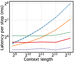
(a) Per-step training latency

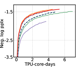
(b) Context length = 512

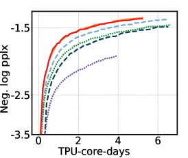
(c) Context length = 1024

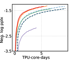
(d) Context length = 2048

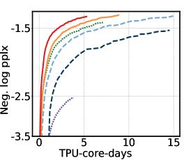
(e) Context length = 4096

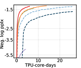
(f) Context length = 8192

Figure 5: Masked language modeling validation-set results on the C4 dataset — All models are comparable in size at around 110M (i.e., BERT-Base scale) and trained for 125K steps with 2¹⁸ tokens per batch. The quality is measured in negative log perplexity.

On Non-overlapping Local Attention.

Chunks in our method does not overlap with each other. In theory, instead of using the non-overlapping local attention, any partial attention variant could be used as a substitute while keeping the chunked linear attention fixed. As a concrete example, we explored allowing each chunk to additionally attends to its nearby chunks, which essentially makes the local attention overlapping, similar to Longformer (Beltagy et al., 2020) and BigBird (Zaheer et al., 2020). While overlapping local attention consistently improves quality, it also introduces many memory re-formatting operations that clearly harm the actual running speed. In our preliminary experiments with language modeling on TPU, we found the cost-benefit trade-off of using overlapping local attention may not be as good as adding more layers in terms of both memory and speed. In general, we believe the optimal partial attention variant is task-specific, while non-overlapping local attention is always a strong candidate when combined with the choice of chunked linear attention.

Connections to Combiner.

Similar to our method, Combiner (Ren et al., 2021) also splits the sequence into non-overlapping chunks and utilizes quadratic local attention within each chunk. The key difference lies in how the long-range information is summarized and combined with the local information (e.g., our mixed chunk attention allows larger effective memory per chunk hence leads to better quality). See Appendix A for detailed discussions.

4 Experiments

We focus on two of our models that have different complexities with respect to the context length. The quadratic-complexity model FLASH-Quad refers to a stack of GAUs whereas the linear-complexity model named FLASH consists of both GAUs and the proposed mixed chunk attention. To demonstrate their efficacy and general applicability, we evaluate them on both bidirectional and auto-regressive sequence modeling tasks over multiple large-scale datasets.

Baselines.

First of all, the vanilla Transformer (Vaswani et al., 2017) with GELU activation function (Hendrycks & Gimpel, 2016) is included as a standard baseline for calibration. Despite of being a popular baseline in the literature, we find that RoPE (Su et al., 2021) and GLU (Shazeer, 2020) can lead to significant performance boosts. We therefore also include Transformer + RoPE (Transformer+) and Transformer + RoPE + GLU (Transformer++) as two much stronger baselines with quadratic complexity.

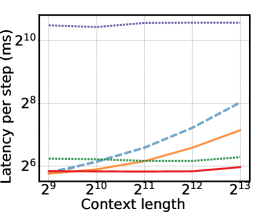
(a) Per-step training latency

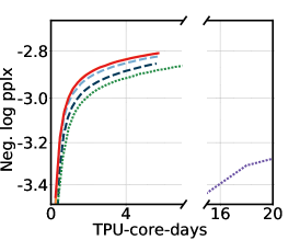
(b) Context length = 512

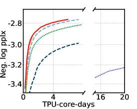
(c) Context length = 1024

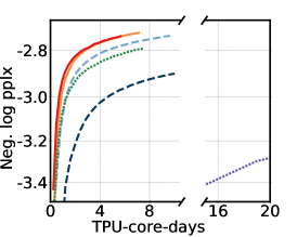
(d) Context length = 2048

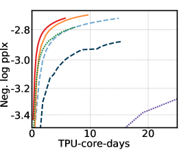
(e) Context length = 4096

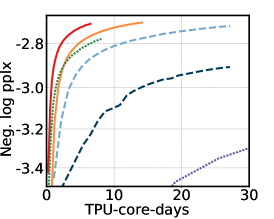
(f) Context length = 8192

Figure 6: Auto-regressive language modeling validation-set results on the Wiki-40B dataset — All models are sized around 110M (i.e., BERT-Base scale) and trained for 125K steps with 2¹⁸ tokens per batch. The quality is measured in negative log perplexity.

To demonstrate the advantages of our models on long sequences, we further compare our models with two notable linear-complexity Transformer variants—Performer (Choromanski et al., 2020) and Combiner (Ren et al., 2021), where Performer is a representative linear attention method and Combiner (using a chunked attention design similar to ours) has shown superior cost-benefit trade-off over many other approaches (Ren et al., 2021). To get the best performance, we use the rowmajor-axial variant of Combiner (Combiner-Axial) and the ReLU-kernel variant of Performer. Both models are also augmented with RoPE.

For fair comparison, all models are implemented in the same codebase to ensure identical tokenizer and hyper-parameters for training and evaluation. The per-step training latencies of all models are measured using TensorFlow Profiler. See Appendix B for detailed settings and model specifications.

4.1 Bidirectional Language Modeling

In BERT (Devlin et al., 2018), masked language modeling (MLM) reconstructs randomly masked out tokens in the input sequence. We pretrain and evaluate all models on the C4 dataset (Raffel et al., 2020). We consistently train each model with $2^{18}$ tokens per batch for 125K steps, while varying the context length on a wide range including 512, 1024, 2048, 4096, and 8192. The quality of each model is reported in perplexity as a proxy metric for the performance on downstream tasks. The training speed of each model (i.e., training latency per step) is measured with 64 TPU-v4 cores, and the total training cost is reported in TPU-v4-core-days.

Figure 5(a) shows the latency of each training step for all models at different context lengths. Results for Transformer+ are omitted for brevity as it lies in between Transformer and Transformer++. Across all the six models, latencies for Combiner, Performer, and FLASH remain roughly constant as the context length increases, demonstrating linear complexity with respect to context length. FLASH-Quad is consistently faster than Transformer and Transformer++ for all context lengths. In particular, FLASH-Quad is 2$\times$ as fast as Transformer++ when the context length increases to 8192. More importantly, as shown in Figures 5(b)-5(f), for all sequence lengths ranging from 512 to 8192, our models always achieve the best quality (i.e., lowest perplexity) under the same computational resource. In particular, if the goal is to match Transformer++’s final perplexity at step 125K, FLASH-Quad and FLASH can reduce the training cost by 1.1$\times$–2.5$\times$ and 1.0$\times$–4.8$\times$, respectively. It is worth noting that, to the best of our knowledge, FLASH is the only linear-complexity model that achieves perplexity competitive with the fully-augmented Transformers and its quadratic-complexity counterpart. See Appendix C.2 for a detailed quality and speed comparison of all models.

4.2 Auto-regressive Language Modeling

Table 3: Auto-regressive language models on the PG-19 dataset — Latency (Lat.) is measured with 64 TPU-v4 cores.

Model	Context Length
	1024			2048			4096			8192
	PPLX	Lat.	Speedup*	PPLX	Lat.	Speedup*	PPLX	Lat.	Speedup*	PPLX	Lat.	Speedup*
Transformer+	44.45	282	1.00$\times$	43.14	433	1.00$\times$	42.80	698	1.00$\times$	43.27	1292	1.00$\times$
Transformer++	44.47	292	–	43.18	441	–	43.13	712	–	43.26	1272	1.21$\times$
Combiner	46.04	386	–	44.68	376	–	43.99	374	–	44.12	407	–
FLASH-Quad	43.40	231	2.18$\times$	42.01	273	$3.29\times$	41.46	371	$3.59\times$	41.68	560	$5.23\times$
FLASH	44.06	234	$1.66\times$	42.17	237	3.85$\times$	40.72	234	6.75$\times$	41.07	250	12.12$\times$

• Measured based on time taken to match Transformer+’s final quality (at step 125K) on TPU.

• Indicates that the specific model fails to achieve the same perplexity as Transformer+.

For auto-regressive language modeling, we focus on the Wiki-40B (Guo et al., 2020) and PG-19 (Rae et al., 2019) datasets, which consist of clean English Wikipedia pages and books extracted from Project Gutenberg, respectively. It is worth noting that the average document length in PG-19 is 69K words, making it ideal for evaluating model performance over long context lengths. We train and evaluate all models with $2^{18}$ tokens per batch for 125K steps, with context lengths ranging from 512 to 8K for Wiki-40B and 1K to 8K for PG-19. We report token-level perplexity for Wiki-40B and word-level perplexity for PG-19.

Figure 6(a) shows that FLASH-Quad and FLASH achieve the lowest latency among quadratic and linear complexity models, respectively. We compare the quality and training cost trade-offs of all models on Wiki40-B over increasing context lengths in Figures 6(b)-6(f). Similar to the findings on MLM tasks, our models dominate all other models in terms of quality-training speed for all sequence lengths. Specifically, FLASH-Quad reduces the training time of Transformer++ by 1.2$\times$ to 2.5$\times$ and FLASH cuts the compute cost by 1.2$\times$ to 4.9$\times$ while reaching a similar perplexity as Transformer++. Between our own models, FLASH closely tracks the perplexity of FLASH-Quad and starts to achieve a better perplexity-cost trade-off when the context length goes beyond 2048. Detailed quality and speed comparisons for all models are included in Appendix C.2.

For PG-19, following Rae et al., an increased model scale of roughly 500M parameters (see Table 10) is used for all models in comparison. The results are summarized in Table 3. Compared to the numbers in Wiki-40B, FLASH achieves a more pronounced improvements in perplexity and training time over the augmented Transformers on PG-19. For example, with a context length of 8K, FLASH-Quad and FLASH are able to reach the final perplexity (at 125K-step) of Transformer+ in only 55K and 55K steps, yielding 5.23$\times$ and 12.12$\times$ of speedup, respectively. We hypothesize that the increased gains over Transformer+ arise from the long-range nature of PG-19 (which consists of books). Similar to our previous experiments, FLASH achieves a lower perplexity than all of the full-attention Transformer variants while being significantly faster, demonstrating the effectiveness of our efficient attention design.

4.3 Fine-tuning

To demonstrate the effectiveness of FLASH over downstream tasks, we fine-tune our pre-trained models on the TriviaQA dataset (Joshi et al., 2017). Passages in TriviaQA can span multiple documents, which challenges the capability of the models in handling long contexts. For a fair and meaningful comparison, we pretrain all models on English Wikipedia (same domain as TriviaQA) with a context length of 4096 and a batch size of 64 for 125k steps. For fine-tuning, we sweep over three different learning rates, including $1e^{-4}$, $7e^{-5}$, and $5e^{-5}$, and report the best validation-set F1 score across these runs.

Table 4: Results on TrivialQA with context length 4096 — “PT“ stands for pre-training and “FT“ stands for fine-tuning. All models are comparable in size at around 110M. $s$ stands for the head size of the single-head attention. For FLASH, “first-to-all” means that we also let the first token in each chunk to attend to the entire sequence using a single-head softmax attention. Latency (Lat.) is measured with 32 TPU-v4 cores.

Model	PT	FT	PT / FT
	PPLX	F1	Lat. reduction
Transformer+	3.48	74.2	1.00$\times$ / 1.00$\times$
Combiner	3.51	67.2	2.78$\times$ / 2.75$\times$
FLASH-Quad$s$=128	3.24	72.7	1.89$\times$ / 1.79$\times$
FLASH-Quad$s$=512	3.12	74.8	1.76$\times$ / 1.67$\times$
FLASH$s$=512	3.23	73.3	2.61$\times$ / 2.60$\times$
FLASH$s$=512 + first-to-all	3.24	73.9	2.78$\times$ / 2.69$\times$

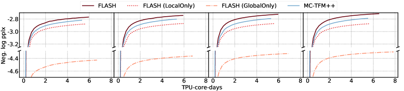
(a) Context length = 1024 (b) Context length = 2048 (c) Context length = 4096 (d) Context length = 8192

Figure 7: Ablation study of the proposed FLASH architecture.

We observe that the fine-tuning results of the FLASH family can benefit from several minor changes in the model configuration. As shown in Table 4, increasing the head size of FLASH-Quad from 128 to 512 leads to a significant boost of 2.1 point in the F1 score with negligible impact on speed. We further identify several other tweaks that improve the linear FLASH variant specifically, including using a small chunk size (128), disabling gradient clipping during finetuning, using softmax instead of squared ReLU for the [CLS] token, and (optionally) allowing the first token in each chunk to attend to the entire sequence using softmax. With those changes, FLASH_$s$=512 achieves comparable quality to Transformer+ (0.3 difference in F1 is within the range of variance) while being 2.8$\times$ and 2.7$\times$ as fast as Transformer+ in pretraining and fine-tuning, respectively.

4.4 Ablation Studies

Significance of quadratic & linear components.

To better understand the efficacy of FLASH, we first study how much the local quadratic attention and the global linear attention contribute to the performance individually. To this end, we create FLASH (LocalOnly) and FLASH (GlobalOnly) by only keeping the local quadratic attention and the global linear attention in FLASH, respectively. In FLASH (GlobalOnly), we reduce the chunk size from 256 to 64 to produce more local summaries for the global linear attention. In Figure 7 we see a significant gap between the full model and the two variants, suggesting that the linear and global attention are complementary to each other — both are critical to the quality of the proposed mixed chunk attention.

Significance of GAU.

Here we study the importance of using GAU in FLASH. To achieve this, we apply the same idea of mixed chunk attention to Transformer++. We refer to this variant as MC-TFM++ (MC stands for mixed chunk) which uses quadratic MHSA within each chunk and multi-head linear attention across chunks. Effectively, MC-TFM++ has the same linear complexity as FLASH, but the core for MC-TFM++ is Transformer++ instead of GAU.

Figure 7 shows that FLASH outperforms MC-TFM++ by a large margin (more than 2$\times$ speedup when the sequence length is greater than 2048), confirming the importance of GAU in our design. We further look into the perplexity increase due to our approximation method in Table 5, showing that the quality loss due to approximation is substantially smaller when going from FLASH-Quad to FLASH than going from TFM++ to MC-TFM++. This indicates that mixed chunk attention is more compatible with GAU than MHSA, which matches our intuition that GAU is more beneficial to weaker/approximate attention mechanisms.

Table 5: Perplexity increases when mixed chunk attention is applied to GAU ($\rightarrow$ FLASH) or to TFM++ ($\rightarrow$ MC-TFM++) — Results are reported for MLM and LM with increasing context lengths from 512 to 8192.

MLM on C4	512	1024	2048	4096	8192
FLASH-Quad $\rightarrow$ FLASH	0.0	0.05	0.06	0.07	0.07
TFM++ $\rightarrow$ MC-TFM++	0.36	0.37	0.49	0.48	0.43
LM on Wiki-40B	512	1024	2048	4096	8192
FLASH-Quad $\rightarrow$ FLASH	-0.05	0.06	0.22	0.30	0.11
TFM++ $\rightarrow$ MC-TFM++	0.54	0.75	0.86	0.90	0.87

Impact of Chunk Size.

The choice of chunk size can affect both the quality and the training cost of FLASH. We observe that, in general, larger chunk sizes perform better as the context length increases. For example, setting the chunk size to 512 is clearly preferable to the default chunk size (C=256) when the context length exceeds 1024. In practice, hyperparameter search over the chunk size can be performed to optimize the performance of FLASH further, although we did not explore such option in our experiments. More detailed analysis can be found in Appendix C.3.

5 Conclusion

We have presented FLASH, a practical solution to address the quality and empirical speed issues of existing efficient Transformer variants. This is achieved by designing a performant layer (gated linear unit) and by combining it with an accelerator-efficient approximation strategy (mixed chunk attention). Experiments on bidirectional and auto-regressive language modeling tasks show that FLASH is as good as fully-augmented Transformers in quality (perplexity), while being substantially faster to train than the state-of-the-art. A future work is to investigate the scaling laws of this new model family and the performance on downstream tasks.

Appendix A Connections to Combiner

To capture long-term information, Combiner (Ren et al., 2021) additionally summarizes each chunk into summary key and value vectors $K^{\text{sum}},V^{\text{sum}}\in\mathbb{R}^{T/C\times d}$ and concatenate them into the local quadratic attention, i.e.

$$\hat{V}_{g}=\mathrm{Softmax}\big{(}Q[K_{g};K^{\text{sum}}]\big{)}[V_{g};V^{\text{sum}}].$$

Effectively, Combiner compresses each chunk of $C$ vectors into a single vector of $\mathcal{O}(d)$, whereas our chunked linear attention part compresses each chunk into a matrix ${K_{h}^{\text{lin}}}^{\top}V_{h}$ of size $\mathcal{O}(sd)$ which is $s$ times larger. In other words, less compression is done in chunked linear attention, allowing increased memory hence a potential advantage over Combiners.

Another difference lies in how the compressed long-term information from different chunks are combined, where Combiner reuses the quadratic attention whereas our chunked linear attention simply performs (cumulative) sum. However, it is straightforward to incorporate what Combiner does in our proposed method by constructing an extra $[T/C\times T/C]$ attention matrix to combine the chunk summaries, e.g.

$$A^{\text{lin}} =\mathrm{relu}^{2}\Big{(}Q^{\text{sum}}{K^{\text{sum}}}^{\top}+b^{\text{sum}}\Big{)},$$

$$\hat{V}_{g}^{\text{lin}} =Q^{\text{lin}}_{g}\bigg{[}\sum_{h=1}^{T/C}a^{\text{lin}}_{gh}\left({K^{\text{lin}}_{h}}^{\top}V_{h}\right)\bigg{]}.$$

We indeed briefly experimented with this variant and found it helpful. But it clearly complicates the overall model design, and more importantly requires the model to store and attend to all chunk summaries. As a result, the auto-regressive decoding complexity will increase to $\mathcal{O}((C+T/C)d^{2})$ which is length-dependent and no longer constant. Hence, we do not include this feature in our default configuration.

Appendix B Experimental Setup

B.1 Hyperparameters

Bidirectional Language Modeling.

Hyperparameters for the MLM task on C4 are listed in Table 6. All models are implemented, trained, and evaluated using the same codebase to guarantee fair comparison.

Table 6: Hyperparameters for MLM pretraining on C4.

	MLM Results (Figure 5)
Data	C4
Sequence length	512 - 8192
Tokens per batch	$2^{18}$
Batch size	$2^{18}/$ Sequence length
Number of steps	125K
Warmup steps	10K
Peak learning rate	7e-4
Learning rate decay	Linear
Optimizer	AdamW
Adam $\epsilon$	1e-6
Adam $(\beta_{1},\beta_{2})$	(0.9, 0.999)
Weight decay	0.01
Local gradient clipping*	0.1
Chunk size	256
Hidden dropout	0
GELU dropout	0
Attention dropout (if applicable)	0

• Applied to all models except the vanilla Transformer.

Auto-regressive Language Modeling.

Hyperparameters for the LM tasks on Wiki-40B and PG-19 are listed in Table 7. All models are implemented, trained, and evaluated using the same codebase to guarantee fair comparison.

Table 7: Hyperparameters for LM pretraining on Wiki-40B and PG-19.

	LM Results (Figure 6)	LM Results (Table 3)
Data	Wiki-40B	PG-19
Sequence length	512 - 8192	1024 - 8192
Tokens per batch	$2^{18}$
Batch size	$2^{18}/$ Sequence length
Number of steps	125K
Warmup steps	10K
Peak learning rate	7e-4
Learning rate decay	Linear
Optimizer	AdamW
Adam $\epsilon$	1e-6
Adam $(\beta_{1},\beta_{2})$	(0.9, 0.999)
Weight decay	0.01
Local gradient clipping*	0.1
Hidden dropout	0
GELU dropout	0
Attention dropout (if applicable)	0
Chunk size	256	512

• Applied to all models except the vanilla Transformer.

B.2 Model Specifications

Detailed specifications of all models used in our experiments are summarized in Tables 8, 9, and 10. In the experiments, SiLU/Swish (Elfwing et al., 2018; Hendrycks & Gimpel, 2016; Ramachandran et al., 2017) is used as the nonlinearity for FLASH-Quad and FLASH, as it slightly outperforms GELU (Hendrycks & Gimpel, 2016) in our models. It is also worth noting that we use ScaleNorm for some masked language models because ScaleNorm runs slightly faster than LayerNorm on TPU-v4 without compromising the quality of the model.

Table 8: Model configurations for MLM experiments on the C4 dataset in Section 4.

	FLASH-Quad	FLASH	Transformer	Transformer+	Transformer++	Combiner	Performer
# of attention heads	1	1	12	12	12	12	12
Attention kernel	relu2	relu2	softmax	softmax	softmax	softmax	relu
Attention type	Quadratic	Mixed Chunk	Quadratic	Quadratic	Quadratic	Rowmajor-Axial	Linear
FFN type	GAU1	GAU1	MLP	MLP	GLU	MLP	MLP
Activation2	SiLU/Swish	SiLU/Swish	GELU	GELU	GELU	GELU	GELU
Norm. type3	ScaleNorm	ScaleNorm	LayerNorm	ScaleNorm	ScaleNorm	ScaleNorm	ScaleNorm
Absolute position emb.	ScaledSin4	ScaledSin4	Learnable5	ScaledSin4	ScaledSin4	ScaledSin4	ScaledSin4
Relative position emb.	RoPE	RoPE	–	RoPE	RoPE	RoPE	RoPE
# of layers	24	24	12+126	12+126	12+126	12+126	12+126
Hidden size	768	768	768	768	768	768	768
Expansion rate	2	2	4	4	4	4	4
Chunk size	–	256	–	–	–	256	–
Params (M)	112	112	110	110	110	124	110

• FLASH-Quad and FLASH combines the attention and feed-forward network into one module named GAU.

• SiLU/Swish are proposed by Elfwing et al. (2018); Hendrycks & Gimpel (2016); Ramachandran et al. (2017).

• ScaleNorm and LayerNorm are proposed by Nguyen & Salazar (2019) and Ba et al. (2016), respectively.

• ScaleSin re-scales sinusoidal position embedding (Vaswani et al., 2017) with a linearnable scalar for stability.

• The learnable position embedding is proposed by Gehring et al. (2017).

• The model is consist of 12 attention layers and 12 FFN layers.

Table 9: Model configurations for LM experiments on the Wiki-40B dataset in Section 4.

	FLASH-Quad	FLASH	Transformer	Transformer+	Transformer++	Combiner	Performer
# of attention heads	1	1	12	12	12	12	12
Attention kernel	relu2	relu2	softmax	softmax	softmax	softmax	relu
Attention type	Quadratic	Mixed Chunk	Quadratic	Quadratic	Quadratic	Rowmajor-Axial	Linear
FFN type	GAU1	GAU1	MLP	MLP	GLU	MLP	MLP
Activation2	SiLU/Swish	SiLU/Swish	GELU	GELU	GELU	GELU	GELU
Norm. type	LayerNorm	LayerNorm	LayerNorm	LayerNorm	LayerNorm	LayerNorm	LayerNorm
Absolute position emb.	ScaledSin3	ScaledSin3	Learnable4	ScaledSin3	ScaledSin3	ScaledSin3	ScaledSin3
Relative position emb.	RoPE	RoPE	–	RoPE	RoPE	RoPE	RoPE
# of layers	24	24	12+125	12+125	12+125	12+125	12+125
Hidden size	768	768	768	768	768	768	768
Expansion rate	2	2	4	4	4	4	4
Chunk size	–	256	–	–	–	256	–
Params (M)	112	112	110	110	110	124	110

• FLASH-Quad and FLASH combines the attention and feed-forward network into one module named GAU.

• SiLU/Swish are proposed by Elfwing et al. (2018); Hendrycks & Gimpel (2016); Ramachandran et al. (2017).

• ScaleSin re-scales sinusoidal position embedding (Vaswani et al., 2017) with a linearnable scalar for stability.

• The learnable position embedding is proposed by Gehring et al. (2017).

• The model is consist of 12 attention layers and 12 FFN layers.

Table 10: Model configurations for LM experiments on the PG-19 dataset in Section 4.

	FLASH-Quad	FLASH	Transformer+	Transformer++	Combiner
# of attention heads	1	1	16	16	16
Attention kernel	relu2	relu2	softmax	softmax	softmax
Attention type	Quadratic	Mixed Chunk	Quadratic	Quadratic	Rowmajor-Axial
FFN type	GAU1	GAU1	MLP	GLU	MLP
Activation2	SiLU/Swish	SiLU/Swish	GELU	GELU	GELU
Norm. type	LayerNorm	LayerNorm	LayerNorm	LayerNorm	LayerNorm
Absolute position emb.	ScaledSin3	ScaledSin3	ScaledSin3	ScaledSin3	ScaledSin3
Relative position emb.	RoPE	RoPE	RoPE	RoPE	RoPE
# of layers	72	72	36+364	36+364	36+364
Hidden size	1024	1024	1024	1024	1024
Expansion rate	2	2	4	4	4
Chunk size	–	512	–	–	512
Params (M)	496	496	486	486	562

• FLASH-Quad and FLASH combines the attention and feed-forward network into one module named GAU.

• SiLU/Swish are proposed by Elfwing et al. (2018); Hendrycks & Gimpel (2016); Ramachandran et al. (2017).

• ScaleSin re-scales sinusoidal position embedding (Vaswani et al., 2017) with a linearnable scalar for stability.

• The model is consist of 36 attention layers and 36 FFN layers.

Appendix C Additional Experimental Results

Here, we provide full results on the training speed of different language models using a Nvidia V100 GPU (in Table 11) and the ablation study of chunk size for FLASH (in Figure 8).

Table 11: Comparison of latency for each training step of auto-regressive language modeling on Wiki-40B using a single Nvidia Tesla V100 GPU — Latency is reported in millisecond. OOM stands for the CUDA out of memory error. Performer-Matmul implements the cumulative sum (cumsum) using matrix multiplication.

	Context length $\times$ Batch size
Model	512 $\times$ 4	1024 $\times$ 2	2048 $\times$ 1	4096 $\times$ 1
Transformer++	222.4	243.9	315.0	OOM
Performer	823.0	827.4	799.8	OOM
Performer-Matmul	697.4	701.7	688.9	OOM
FLASH	254.4	235.0	242.8	452.9

C.1 Auto-regressive Training on GPU

We observe that the inefficiency of auto-regressive training is not limited to hardware accelerators such as TPUs. As shown in Table 11, Performer has the largest latency among the three models because it requires to perform cumsum over all tokens sequentially. In contrast, the proposed FLASH achieves the lowest latency when the context length is over 1024, suggesting the effectiveness of the proposed mixed chunk attention mechanism.

C.2 Tabular MLM and LM Results

We summarize the experimental results of MLM on C4 and LM on Wiki-40B in Tables 12 and 13.

Table 12: Bidirectional/masked language models on the C4 dataset. The best perplexity (PPLX) on the validation set is reported. Training latency is measured with 64 TPU-v4 cores.

Model	Context Length
	512		1024		2048		4096		8192
	PPLX	Latency	PPLX	Latency	PPLX	Latency	PPLX	Latency	PPLX	Latency
Transformer	4.517	47.7	4.436	63.9	4.196	90.9	4.602	142.5	4.8766	252.7
Transformer+	4.283	48.8	4.151	64.4	4.032	91.5	3.989	142.9	3.986	252.9
Transformer++	4.205	47.6	4.058	64.6	3.920	91.6	3.876	143.4	3.933	252.1
Performer	5.897	37.2	6.324	37.6	8.032	39.1	12.622	36.9	102.980	40.9
Combiner	4.449	67.2	4.317	66.4	4.238	66.4	4.195	68.3	4.225	77.3
FLASH-Quad	4.176	43.7	3.964	50.1	3.864	61.7	3.828	84.9	3.830	132.1
FLASH	4.172	51.2	4.015	50.1	3.928	51.4	3.902	50.7	3.897	59.9

Table 13: Auto-regressive language models on the Wiki-40B dataset. The best perplexity (PPLX) on the validation set is reported. Training latency is measured with 64 TPU-v4 cores.

Model	Context Length
	512		1024		2048		4096		8192
	PPLX	Latency	PPLX	Latency	PPLX	Latency	PPLX	Latency	PPLX	Latency
Transformer	17.341	54.0	19.808	70.9	18.154	96.3	17.731	149.1	18.254	260.7
Transformer+	16.907	55.6	15.999	70.3	15.653	96.1	15.515	149.3	15.478	261.9
Transformer++	16.835	54.7	15.943	70.9	15.489	96.6	15.282	149.2	15.254	261.0
Performer	18.989	1439.7	18.520	1386.9	18.547	1518.9	18.987	1526.7	19.923	1526.8
Combiner	17.338	75.5	16.710	74.4	16.344	71.8	16.171	71.7	16.119	77.9
FLASH-Quad	16.633	54.1	15.879	59.5	15.305	71.3	14.955	96.1	14.998	141.3
FLASH	16.581	57.2	15.935	56.9	15.525	56.7	15.259	57.0	15.109	62.5

C.3 Ablation Study of Chunk Size

The choice of chunk size can have an impact on both the quality and the training cost of FLASH. In the extreme case where chunk size equals the context length, FLASH falls back to FLASH-Quad and loses the scalability to long context lengths. In the other extreme case where chunk size is equal to one, the proposed attention module becomes a linear attention, which suffers from inefficient auto-regressive training. Figure 8 shows the tradeoff between the quality and training cost of four different chunk sizes for context lengths from 1K to 8K.

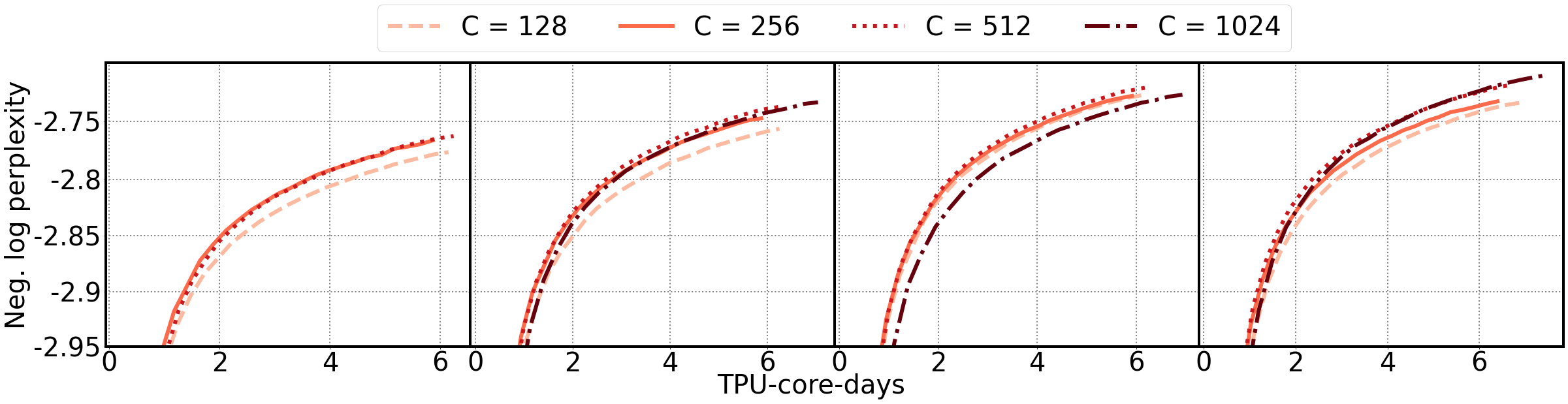
(a) Context length = 1024 (b) Context length = 2048 (c) Context length = 4096 (d) Context length = 8192

Figure 8: Ablation study of the chunk size (C) of FLASH for context lengths from 1K to 8K.

Appendix D Pseudocode For FLASH-Quad and FLASH

We show the detailed implementation of FLASH-Quad and FLASH in Codes 6 and 8.

⬇

def _get_scaledsin(embeddings):

"""Create␣sinusoidal␣position␣embedding␣with␣a␣scaling␣factor."""

hidden_size = int(embeddings.shape[-1])

pos = tf.range(tf.shape(embeddings)[1])

pos = tf.cast(pos, tf.float32)

half_d = hidden_size // 2

freq_seq = tf.cast(tf.range(half_d), tf.float32) / float(half_d)

inv_freq = 10000 ** -freq_seq

sinusoid = tf.einsum('s,d$\rightarrow$sd', pos, inv_freq)

scaledsin = tf.concat([tf.sin(sinusoid), tf.cos(sinusoid)], axis=-1)

scalar = tf.get_variable(

'scaledsin_scalar',

shape=(),

initializer=tf.constant_initializer(1 / hidden_size ** 0.5))

scaledsin *= scalar

return scaledsin

Code 2 Pseudocode for ScaledSin absolute position embedding.

⬇

def rope(x, axis):

"""RoPE␣position␣embedding."""

shape = x.shape.as_list()

if isinstance(axis, int):

axis = [axis]

spatial_shape = [shape[i] for i in axis]

total_len = 1

for i in spatial_shape:

total_len *= i

position = tf.reshape(

tf.cast(tf.range(total_len, delta=1.0), tf.float32), spatial_shape)

for i in range(axis[-1] + 1, len(shape) - 1, 1):

position = tf.expand_dims(position, axis=-1)

half_size = shape[-1] // 2

freq_seq = tf.cast(tf.range(half_size), tf.float32)/float(half_size)

inv_freq = 10000 ** -freq_seq

sinusoid = tf.einsum('…,d$\rightarrow$…d', position, inv_freq)

sin = tf.sin(sinusoid)

cos = tf.cos(sinusoid)

x1, x2 = tf.split(x, 2, axis=-1)

return tf.concat([x1 * cos - x2 * sin, x2 * cos + x1 * sin], axis=-1)

Code 3 Pseudocode for RoPE.

⬇

WEIGHT_INITIALIZER = tf.random_normal_initializer(stddev=0.02)

def rel_pos_bias(n):

"""Relative␣position␣bias."""

if n < 512:

# Construct Toeplitz matrix directly when the sequence length is less than 512.

w = tf.get_variable(

'weight',

shape=[2 * n - 1],

dtype=tf.float32,

initializer=WEIGHT_INITIALIZER)

t = tf.pad(w, [[0, n]])

t = tf.tile(t, [n])

t = t[…, :-n]

t = tf.reshape(t, [n, 3 * n - 2])

r = (2 * n - 1) // 2

t = t[…, r:-r]

else:

# Construct Toeplitz matrix using RoPE when the sequence length is over 512.

a = tf.get_variable(

'a',

shape=[128],

dtype=dtype,

initializer=WEIGHT_INITIALIZER)

b = tf.get_variable(

'b',

shape=[128],

dtype=dtype,

initializer=WEIGHT_INITIALIZER)

a = rope(tf.tile(a[None, :], [n, 1]), axis=0)

b = rope(tf.tile(b[None, :], [n, 1]), axis=0)

t = tf.einsum('mk,nk$\rightarrow$mn', a, b)

return t

Code 4 Pseudocode for relative position bias.

⬇

def norm(x, begin_axis=-1, eps=1e-5, norm_type='layer_norm'):

"""Normalization␣layer."""

shape = x.shape.as_list()

axes = list(range(len(shape)))[begin_axis:]

if norm_type == 'layer_norm':

mean, var = tf.nn.moments(x, axes, keepdims=True)

x = (x - mean) * tf.rsqrt(var + eps)

gamma = tf.get_variable(

'gamma', shape=x.shape.as_list()[begin_axis:], initializer=tf.initializers.ones())

beta = tf.get_variable(

'beta', shape=x.shape.as_list()[begin_axis:], initializer=tf.initializers.zeros())

return gamma * x + beta

elif norm_type == 'scale_norm':

mean_square =tf.reduce_mean(tf.math.square(x), axes, keepdims=True)

x = x * tf.rsqrt(mean_square + eps)

scalar = tf.get_variable('scalar', shape=(), initializer=tf.constant_initializer(1.0))

return scale * x

Code 5 Pseudocode for LayerNorm and ScaleNorm.

⬇

WEIGHT_INITIALIZER = tf.random_normal_initializer(stddev=0.02)

def GAU(x, causal, norm_type='layer_norm', expansion_factor=2):

"""GAU␣block.

␣␣␣␣Input␣shape:␣batch␣size␣x␣sequence␣length␣x␣model␣size

␣␣␣␣"""

seq_len = tf.shape(x)[1]

d = int(x.shape[-1])

e = int(d * expansion_factor)

shortcut, x = x, norm(x, begin_axis=-1, norm_type=norm_type)

s = 128

uv = tf.layers.dense(x, 2 * e + s, kernel_initializer=WEIGHT_INITIALIZER, bias_initializer='zeros')

u, v, base = tf.split(tf.nn.silu(uv), [e, e, s], axis=-1)

# Generate Query (q) and Key (k) from base.

gamma = tf.get_variable('gamma', shape=[2, s], initializer=WEIGHT_INITIALIZER)

beta = tf.get_variable('beta', shape=[2, s], initializer=tf.initializers.zeros())

base = tf.einsum('…r,hr$\rightarrow$…hr', base, gamma) + beta

base = rope(base, axis=1)

q, k = tf.unstack(base, axis=-2)

# Calculate the quadratic attention.

qk = tf.einsum('bnd,bmd$\rightarrow$bnm', q, k)

bias = rel_pos_bias(seq_len)

kernel = tf.math.square(tf.nn.relu(qk / seq_len + bias))

# Apply the causal mask for auto-regressive tasks.

if causal:

causal_mask = tf.linalg.band_part(

tf.ones([seq_len, seq_len], dtype=x.dtype), num_lower=-1, num_upper=0)

kernel *= causal_mask

x = u * tf.einsum('bnm,bme$\rightarrow$bne', kernel, v)

x = tf.layers.dense(x, d, kernel_initializer=WEIGHT_INITIALIZER, bias_initializer='zeros')

return x + shortcut

Code 6 Pseudocode for GAU (FLASH-Quad).

⬇

def segment_ids_to_mask(segment_ids, causal=False):

"""Generate␣the␣segment␣mask␣from␣the␣segment␣ids.

␣␣␣␣The␣segment␣mask␣is␣used␣to␣remove␣the␣attention␣between␣tokens␣in␣different␣documents.

␣␣␣␣"""

min_ids, max_ids = tf.reduce_min(segment_ids, axis=-1), tf.reduce_max(segment_ids, axis=-1)

# 1.0 indicates in the same group and 0.0 otherwise

mask = tf.logical_and(

tf.less_equal(min_ids[:, :, None], max_ids[:, None, :]),

tf.greater_equal(max_ids[:, :, None], min_ids[:, None, :]))

mask = tf.cast(mask, tf.float32)

if causal:

g = tf.shape(min_ids)[1]

causal_mask = 1.0 - tf.linalg.band_part(

tf.ones([g, g], dtype=tf.float32), num_lower=0, num_upper=-1)

mask *= causal_mask

mask = tf.math.divide_no_nan(mask, tf.reduce_sum(mask, axis=-1, keepdims=True))

return mask

Code 7 Pseudocode for generating segment mask.

⬇

WEIGHT_INITIALIZER = tf.random_normal_initializer(stddev=0.02)

def FLASH(x, causal, segment_ids, norm_type='layer_norm', expansion_factor=2):

"""FLASH␣block.

␣␣␣␣Input␣shape:␣batch␣size␣x␣num␣chunks␣x␣chunk␣length␣x␣model␣size

␣␣␣␣"""

_, g, n, d = x.shape.as_list()

e = int(d * expansion_factor)

shortcut, x = x, norm(x, begin_axis=-1, norm_type=norm_type)

s = 128

uv = tf.layers.dense(x, 2 * e + s, kernel_initializer=WEIGHT_INITIALIZER, bias_initializer='zeros')

u, v, base = tf.split(tf.nn.silu(uv), [e, e, s], axis=-1)

# Generate Query and Key for both quadratic and linear attentions.

gamma = tf.get_variable('gamma', shape=[4, s], initializer=WEIGHT_INITIALIZER)

beta = tf.get_variable('beta', shape=[4, s], initializer=tf.initializers.zeros())

base = tf.einsum('…r,hr$\rightarrow$…hr', base, gamma) + beta

base = rope(base, axis=[1, 2])

quad_q, quad_k, lin_q, lin_k = tf.unstack(base, axis=-2)

if causal:

# Linear attention part.

lin_kv = tf.einsum('bgnk,bgne$\rightarrow$bgke', lin_k, v) / tf.cast(n, x.dtype)

mask = segment_ids_to_mask(segment_ids, causal=True)

cum_lin_kv = tf.einsum('bhke,bgh$\rightarrow$bgke', lin_kv, mask)

linear = tf.einsum('bgnk,bgke$\rightarrow$bgne', lin_q, cum_lin_kv)

# Quadratic attention part.

quad_qk = tf.einsum('bgnk,bgmk$\rightarrow$bgnm', quad_q, quad_k)

bias = rel_pos_bias(n)

kernel = tf.math.square(tf.nn.relu(quad_qk / n + bias))

# Apply the causal mask for auto-regressive tasks.

causal_mask = tf.linalg.band_part(tf.ones([n, n], dtype=x.dtype), num_lower=-1, num_upper=0)

quadratic = tf.einsum('bgnm,bgme$\rightarrow$bgne', kernel * causal_mask, v)

else:

# Linear attention part

lin_kv = tf.einsum('bgnk,bgne$\rightarrow$bgke', lin_k, v) / tf.cast(n, x.dtype)

mask = segment_ids_to_mask(segment_ids)

lin_kv = tf.einsum('bhke,bgh$\rightarrow$bgke', lin_kv, mask)

linear = tf.einsum('bgnk,bgke$\rightarrow$bgne', lin_q, lin_kv)

# Quadratic attention part

quad_qk = tf.einsum('bgnk,bgmk$\rightarrow$bgnm', quad_q, quad_k)

bias = rel_pos_bias(n)

kernel = tf.math.square(tf.nn.relu((quad_qk / n + bias))

quadratic = tf.einsum('bgnm,bgme$\rightarrow$bgne', kernel, v)

x = u * (quadratic + linear)

x = tf.layers.dense(x, d, kernel_initializer=WEIGHT_INITIALIZER, bias_initializer='zeros')

return x + shortcut

Code 8 Pseudocode for FLASH.

References

- Ba et al. (2016) Ba, J. L., Kiros, J. R., and Hinton, G. E. Layer normalization. arXiv preprint arXiv:1607.06450, 2016.
- Beltagy et al. (2020) Beltagy, I., Peters, M. E., and Cohan, A. Longformer: The long-document transformer. arXiv preprint arXiv:2004.05150, 2020.
- Brown et al. (2020) Brown, T. B., Mann, B., Ryder, N., Subbiah, M., Kaplan, J., Dhariwal, P., Neelakantan, A., Shyam, P., Sastry, G., Askell, A., et al. Language models are few-shot learners. arXiv preprint arXiv:2005.14165, 2020.
- Child et al. (2019) Child, R., Gray, S., Radford, A., and Sutskever, I. Generating long sequences with sparse transformers. arXiv preprint arXiv:1904.10509, 2019.
- Choromanski et al. (2020) Choromanski, K., Likhosherstov, V., Dohan, D., Song, X., Gane, A., Sarlos, T., Hawkins, P., Davis, J., Mohiuddin, A., Kaiser, L., et al. Rethinking attention with performers. arXiv preprint arXiv:2009.14794, 2020.
- Dai et al. (2019) Dai, Z., Yang, Z., Yang, Y., Carbonell, J., Le, Q. V., and Salakhutdinov, R. Transformer-xl: Attentive language models beyond a fixed-length context. arXiv preprint arXiv:1901.02860, 2019.
- Dauphin et al. (2017) Dauphin, Y. N., Fan, A., Auli, M., and Grangier, D. Language modeling with gated convolutional networks. In Proceedings of the 34th International Conference on Machine Learning - Volume 70, ICML’17, pp. 933–941. JMLR.org, 2017.
- Devlin et al. (2018) Devlin, J., Chang, M.-W., Lee, K., and Toutanova, K. Bert: Pre-training of deep bidirectional transformers for language understanding. arXiv preprint arXiv:1810.04805, 2018.
- Dosovitskiy et al. (2020) Dosovitskiy, A., Beyer, L., Kolesnikov, A., Weissenborn, D., Zhai, X., Unterthiner, T., Dehghani, M., Minderer, M., Heigold, G., Gelly, S., et al. An image is worth 16x16 words: Transformers for image recognition at scale. arXiv preprint arXiv:2010.11929, 2020.
- Du et al. (2021) Du, N., Huang, Y., Dai, A. M., Tong, S., Lepikhin, D., Xu, Y., Krikun, M., Zhou, Y., Yu, A. W., Firat, O., et al. Glam: Efficient scaling of language models with mixture-of-experts. arXiv preprint arXiv:2112.06905, 2021.
- Elfwing et al. (2018) Elfwing, S., Uchibe, E., and Doya, K. Sigmoid-weighted linear units for neural network function approximation in reinforcement learning. Neural Networks, 107:3–11, 2018.
- Gehring et al. (2017) Gehring, J., Auli, M., Grangier, D., Yarats, D., and Dauphin, Y. N. Convolutional sequence to sequence learning. In Proceedings of the 34th International Conference on Machine Learning - Volume 70, ICML’17, pp. 1243–1252. JMLR.org, 2017.
- Guo et al. (2020) Guo, M., Dai, Z., Vrandecic, D., and Al-Rfou, R. Wiki-40b: Multilingual language model dataset. In LREC 2020, 2020.
- Hendrycks & Gimpel (2016) Hendrycks, D. and Gimpel, K. Gaussian error linear units (gelus). arXiv preprint arXiv:1606.08415, 2016.
- Ho et al. (2019) Ho, J., Kalchbrenner, N., Weissenborn, D., and Salimans, T. Axial attention in multidimensional transformers. arXiv preprint arXiv:1912.12180, 2019.
- Huang et al. (2019) Huang, Z., Wang, X., Huang, L., Huang, C., Wei, Y., and Liu, W. Ccnet: Criss-cross attention for semantic segmentation. In Proceedings of the IEEE/CVF International Conference on Computer Vision, pp. 603–612, 2019.
- Jaegle et al. (2021) Jaegle, A., Gimeno, F., Brock, A., Vinyals, O., Zisserman, A., and Carreira, J. Perceiver: General perception with iterative attention. In International Conference on Machine Learning, pp. 4651–4664. PMLR, 2021.
- Joshi et al. (2017) Joshi, M., Choi, E., Weld, D., and Zettlemoyer, L. TriviaQA: A large scale distantly supervised challenge dataset for reading comprehension. In Proceedings of the 55th Annual Meeting of the Association for Computational Linguistics (Volume 1: Long Papers), pp. 1601–1611, Vancouver, Canada, July 2017. Association for Computational Linguistics. doi: 10.18653/v1/P17-1147. URL https://aclanthology.org/P17-1147.
- Katharopoulos et al. (2020) Katharopoulos, A., Vyas, A., Pappas, N., and Fleuret, F. Transformers are rnns: Fast autoregressive transformers with linear attention. In International Conference on Machine Learning, pp. 5156–5165. PMLR, 2020.
- Kitaev et al. (2020) Kitaev, N., Kaiser, Ł., and Levskaya, A. Reformer: The efficient transformer. arXiv preprint arXiv:2001.04451, 2020.
- Li et al. (2019) Li, S., Jin, X., Xuan, Y., Zhou, X., Chen, W., Wang, Y.-X., and Yan, X. Enhancing the locality and breaking the memory bottleneck of transformer on time series forecasting. Advances in Neural Information Processing Systems, 32:5243–5253, 2019.
- Liu et al. (2021) Liu, H., Dai, Z., So, D. R., and Le, Q. V. Pay attention to mlps. NeurIPS, 2021.
- Narang et al. (2021) Narang, S., Chung, H. W., Tay, Y., Fedus, W., Fevry, T., Matena, M., Malkan, K., Fiedel, N., Shazeer, N., Lan, Z., et al. Do transformer modifications transfer across implementations and applications? arXiv preprint arXiv:2102.11972, 2021.
- Nguyen & Salazar (2019) Nguyen, T. Q. and Salazar, J. Transformers without tears: Improving the normalization of self-attention. CoRR, abs/1910.05895, 2019. URL http://arxiv.org/abs/1910.05895.
- Peng et al. (2021) Peng, H. et al. Random feature attention. In ICLR, 2021.
- Rae et al. (2019) Rae, J. W., Potapenko, A., Jayakumar, S. M., and Lillicrap, T. P. Compressive transformers for long-range sequence modelling. arXiv preprint arXiv:1911.05507, 2019.
- Raffel et al. (2020) Raffel, C., Shazeer, N., Roberts, A., Lee, K., Narang, S., Matena, M., Zhou, Y., Li, W., and Liu, P. J. Exploring the limits of transfer learning with a unified text-to-text transformer. Journal of Machine Learning Research, 21(140):1–67, 2020. URL http://jmlr.org/papers/v21/20-074.html.
- Ramachandran et al. (2017) Ramachandran, P., Zoph, B., and Le, Q. V. Searching for activation functions. CoRR, abs/1710.05941, 2017. URL http://arxiv.org/abs/1710.05941.
- Ren et al. (2021) Ren, H., Dai, H., Dai, Z., Yang, M., Leskovec, J., Schuurmans, D., and Dai, B. Combiner: Full attention transformer with sparse computation cost. In Beygelzimer, A., Dauphin, Y., Liang, P., and Vaughan, J. W. (eds.), Advances in Neural Information Processing Systems, 2021. URL https://openreview.net/forum?id=MQQeeDiO5vv.
- Roy et al. (2021) Roy, A., Saffar, M., Vaswani, A., and Grangier, D. Efficient content-based sparse attention with routing transformers. Transactions of the Association for Computational Linguistics, 9:53–68, 2021.
- Shazeer (2020) Shazeer, N. GLU variants improve transformer. CoRR, abs/2002.05202, 2020. URL https://arxiv.org/abs/2002.05202.
- So et al. (2021) So, D. R., Mańke, W., Liu, H., Dai, Z., Shazeer, N., and Le, Q. V. Primer: Searching for efficient transformers for language modeling. NeurIPS, 2021.
- Su et al. (2021) Su, J., Lu, Y., Pan, S., Wen, B., and Liu, Y. Roformer: Enhanced transformer with rotary position embedding, 2021.
- Thoppilan et al. (2022) Thoppilan, R., De Freitas, D., Hall, J., Shazeer, N., Kulshreshtha, A., Cheng, H.-T., Jin, A., Bos, T., Baker, L., Du, Y., et al. Lamda: Language models for dialog applications. arXiv preprint arXiv:2201.08239, 2022.
- Vaswani et al. (2017) Vaswani, A., Shazeer, N., Parmar, N., Uszkoreit, J., Jones, L., Gomez, A. N., Kaiser, Ł., and Polosukhin, I. Attention is all you need. In Advances in neural information processing systems, pp. 5998–6008, 2017.
- Wang et al. (2020) Wang, S., Li, B. Z., Khabsa, M., Fang, H., and Ma, H. Linformer: Self-attention with linear complexity. arXiv preprint arXiv:2006.04768, 2020.
- Zaheer et al. (2020) Zaheer, M., Guruganesh, G., Dubey, K. A., Ainslie, J., Alberti, C., Ontanon, S., Pham, P., Ravula, A., Wang, Q., Yang, L., et al. Big bird: Transformers for longer sequences. In NeurIPS, 2020.