Pion-induced radiative corrections to neutron beta-decay

Abstract

We compute the electromagnetic corrections to neutron beta decay using a low-energy hadronic effective field theory. We identify and compute new radiative corrections arising from virtual pions that were missed in previous studies. The largest correction is a percent-level shift in the axial charge of the nucleon proportional to the electromagnetic part of the pion-mass splitting. Smaller corrections, comparable to anticipated experimental precision, impact the $\beta$-$\nu$ angular correlations and the $\beta$-asymmetry. We comment on implications of our results for the comparison of the experimentally measured axial charge with first-principle computations using lattice QCD and on the potential of $\beta$-decay experiments to constrain beyond-the-Standard-Model interactions.

Introduction — High-precision measurements of low-energy processes, such as $\beta$ decays of mesons, neutron, and nuclei, probe the existence of new physics at very high energy scales through quantum fluctuations. Recent developments in the study of $\beta$ decay rates at the sub-% level Seng et al. (2018, 2019); Czarnecki et al. (2019); Shiells et al. (2021); Hardy and Towner (2020) have led to a 3-5$\sigma$ tension with the Standard Model (SM) interpretation in terms of the unitary Cabibbo-Kobayashi-Maskawa (CKM) quark mixing matrix Hardy and Towner (2020); Zyla et al. (2020). Further, global analyses of $\beta$ decay observables Falkowski et al. (2020); González-Alonso et al. (2019) have highlighted additional avenues for $\beta$ decays to probe physics beyond the Standard Model (BSM) at the multi-TeV scale, such as the comparison of the experimentally extracted weak axial charge, $g_{A}$, with precise lattice Quantum ChromoDynamics (QCD) calculations Bhattacharya et al. (2012); Alioli et al. (2017); Chang et al. (2018). This test is a unique and sensitive probe of BSM right-handed charged currents.

Given the expected improvements in experimental precision in the next few years Cirigliano et al. (2019); Počanić et al. (2009); Dubbers et al. (2008), a necessary condition to use neutron decay as probe of BSM physics is to have high-precision calculations within the SM, including sub-% level recoil and radiative corrections with controlled uncertainties. These prospects have spurred new theoretical activity, which has focused first on radiative corrections to the strength of the Fermi transition (vector coupling) Seng et al. (2018, 2019); Czarnecki et al. (2019); Shiells et al. (2021), and more recently on the corrections to the Gamow-Teller (axial) coupling Hayen (2021); Gorchtein and Seng (2021). These recent studies are all rooted in the current algebra approach developed in the sixties and seventies Sirlin (1967, 1978), combined with the novel use of dispersive techniques.

In principle, lattice QCD can be used to compute the full Standard Model $n\rightarrow pe\bar{\nu}$ decay amplitude including radiative QED corrections, similar to the determination of the leptonic pion decay rate Carrasco et al. (2015); Giusti et al. (2018). However, it will be some years before these calculations reach sufficient precision. Currently, lattice QCD calculations are carried out in the isospin limit. The global average determination of $g_{A}$ carries a 2.2% uncertainty Aoki et al. (2021) with one result achieving a 0.74% uncertainty Chang et al. (2018); Walker-Loud et al. (2020). The PDG average value, on the other hand, has an 0.1% uncertainty Zyla et al. (2020) with the most precise experiment having an 0.035% uncertainty Märkisch et al. (2019).

In this work, we perform a systematic study of neutron decay using effective field theory (EFT). We compute new structure-dependent electromagnetic corrections originating at the pion mass scale, including effects of $\mathcal{O}(\alpha)$ and $\mathcal{O}(\alpha m_{\pi}/m_{N})$, with $\alpha=e^{2}/4\pi$ the fine-structure constant and $m_{\pi}(m_{N})$ the pion (nucleon) mass. By doing so we uncover new percent-level electromagnetic corrections to the axial coupling $g_{A}$, which were missed both in the only other neutron $\beta$ decay EFT analysis  Ando et al. (2004) and recent dispersive treatments Hayen (2021); Gorchtein and Seng (2021).

Neutron decay from the Standard Model — The energy release in neutron decay is roughly the mass splitting of the neutron and proton, i.e. $q_{\mathrm{ext}}\sim m_{n}-m_{p}\sim 1$ MeV, which is significantly smaller than the nucleon mass. The energy scale of nucleon structure corrections, on the other hand, is related to the pion mass, so that $m_{N}\gg m_{\pi}\gg m_{n}-m_{p}$. Large scale separations, such as these, make for ideal systems for an EFT description.

As a consequence, corrections to neutron $\beta$ decay can be parametrized in terms of two small parameters: ($i$) $\epsilon_{\rm recoil}=q_{\rm ext}/m_{N}\sim 0.1\%$ which characterizes small kinetic corrections; ($ii$) $\epsilon_{{/\pi}}=q_{\rm ext}/m_{\pi}\sim 1\%$, which characterizes nucleon structure corrections dominated by radiative pion contributions. At these relatively low energies, the decay amplitude can be described by a non-relativistic Lagrangian density (see also Refs. Ando et al. (2004); Falkowski et al. (2021))

$$\mathcal{L}_{{/\pi}} =-\sqrt{2}G_{F}V_{ud}\,\bigg{[}\bar{e}\gamma_{\mu}P_{L}\nu_{e}\bigg{(}\bar{N}\left(g_{V}v_{\mu}-2g_{A}S_{\mu}\right)\tau^{+}N$$

$$+\frac{i}{2m_{N}}\bar{N}(v^{\mu}v^{\nu}-g^{\mu\nu}-2g_{A}v^{\mu}S^{\nu})(\overleftarrow{\partial}-\overrightarrow{\partial})_{\nu}\tau^{+}N\bigg{)}$$

$$+\frac{ic_{T}m_{e}}{m_{N}}\bar{N}\left(S^{\mu}v^{\nu}-S^{\nu}v^{\mu}\right)\tau^{+}N\,\left(\bar{e}\sigma_{\mu\nu}P_{L}\nu\right)\,$$

$$+\frac{i\mu_{\rm weak}}{m_{N}}\bar{N}[S^{\mu},S^{\nu}]\tau^{+}N\,\partial_{\nu}\left(\bar{e}\gamma_{\mu}P_{L}\nu\right)\bigg{]}+\dots$$ (1)

where pions have been integrated out (hence subscript ${/\pi}$), and the ellipsis denote terms not affected by our analysis. In this expression, $N^{T}=(p,n)$ is an isodoublet of nucleons, while $v_{\mu}$ and $S_{\mu}$ represent the velocity and spin of the nucleon, respectively. The effective vector and axial-vector couplings $g_{V,A}$ are related, as discussed below, to the isovector nucleon vector and axial charges, while $\mu_{\rm weak}$ and $c_{T}$ are the weak magnetic moment and an effective tensor coupling, respectively. The Lagrangian (Pion-induced radiative corrections to neutron beta-decay) can be used to compute the differential neutron decay rate and the parameters can then be fitted to data.

There are a number of short-comings to this approach. First, by utilizing measured values of $V_{ud}\,g_{V}$, $g_{A}/g_{V}$, $\mu_{\rm weak}$, and $c_{T}$, we cannot extract fundamental SM parameters nor distinguish SM from BSM contributions to these low-energy constants (LECs). Second, it is not possible to disentangle, for example, how much of $g_{A}$ arises from isospin symmetric QCD versus electromagnetic contributions. Therefore, it is desirable to utilize an EFT Lagrangian which encodes the corrections as functions of the SM parameters, such as the quark masses and the electromagnetic couplings. This is known as chiral perturbation theory ($\chi$PT) Gasser and Leutwyler (1984, 1985), or specifically for baryons, heavy baryon $\chi$PT (HB$\chi$PT) Jenkins and Manohar (1991). The cost of such a description is the introduction of new scales, $m_{\pi}$ and $\Lambda_{\chi}=4\pi F_{\pi}\sim 1$ GeV with $F_{\pi}\simeq 92.4$ MeV, which form another expansion parameter, $\epsilon_{\chi}=m_{\pi}/\Lambda_{\chi}$, and new operators with potentially undetermined LECs.

Radiative corrections to neutron decay can be organized in a double expansion in $\alpha\epsilon^{n}_{\chi}\epsilon^{m}_{/\pi}$. First, we integrate out the pions and match the $\chi$PT amplitude to the ${/\pi}$EFT amplitude, thus determining the quark mass and electromagnetic corrections to effective couplings such as $g_{A}$. Then, the neutron decay amplitude can be computed with ${/\pi}$EFT (with dynamical photons and leptons) while retaining explicit sensitivity to the parameters of the Standard Model. In our analysis of the decay amplitude we retain terms of $\mathcal{O}(G_{F}\epsilon_{\rm recoil})$, known in the literature, $\mathcal{O}(G_{F}\alpha)$, where we uncover previously overlooked effects, and terms of $\mathcal{O}(G_{F}\alpha\epsilon_{\chi})$ and $\mathcal{O}(G_{F}\alpha\epsilon_{{/\pi}})$, never before considered in the literature.

$\chi$PT setup for neutron decay — To study radiative corrections to weak semi-leptonic transitions, we adopt the HB$\chi$PT framework Jenkins and Manohar (1991) with dynamical photons Meißner and Steininger (1998); Muller and Meißner (1999); Gasser et al. (2002) and leptons, in analogy with the meson sector Knecht et al. (2000). This EFT provides a necessary intermediate step in the analysis of neutron decay, before integrating out pions, and is the starting point for the study of related processes such as muon capture, low-energy neutrino-nucleus scattering, and nuclear $\beta$ decays, which of course require a non-trivial generalization to multi-nucleon effects.

In $\chi$PT with dynamical photons and leptons, semileptonic amplitudes are expanded in the Fermi constant $G_{F}$ (to first order), the electromagnetic fine structure constant $\alpha$, and $\epsilon_{\chi}$, while keeping all orders in $q_{\rm ext}/m_{\pi}$, according to Weinberg’s power counting Weinberg (1979, 1990, 1991). Following standard practice, derivatives ($\partial\sim p$) and the electroweak couplings $e$, $G_{F}$ are assigned chiral dimension one, while the light quark mass is assigned chiral dimension two ($m_{\pi}^{2}\sim p^{2}$). The relevant effective Lagrangians, ordered according to their chiral dimension, are

$${\cal L}_{\pi} = {\cal L}_{\pi}^{(2)}+...$$ (2a)

$${\cal L}_{\pi N} = {\cal L}_{\pi N}^{(1)}+{\cal L}_{\pi N}^{(2)}+{\cal L}_{\pi N}^{(3)}+...$$ (2b)

$${\cal L}_{\rm lept} \equiv {\cal L}_{\rm lept}^{(1)}=\bar{e}\left(i\not{\partial}+e\not{A}-m_{e}\right)e+\bar{\nu}i\not{\partial}\nu~{}.$$ (2c)

At a given chiral dimension, one can further separate the strong and electromagnetic Lagrangians

$${\cal L}_{\pi}^{(2)} = {\cal L}_{\pi}^{p^{2}}+{\cal L}_{\pi}^{e^{2}p^{0}}$$ (3a)

$${\cal L}_{\pi N}^{(1)} = {\cal L}_{\pi N}^{p}$$ (3b)

$${\cal L}_{\pi N}^{(2)} = {\cal L}_{\pi N}^{p^{2}}+{\cal L}_{\pi N}^{e^{2}p^{0}}$$ (3c)

$${\cal L}_{\pi N}^{(3)} = {\cal L}_{\pi N}^{p^{3}}+{\cal L}_{\pi N}^{e^{2}p}+{\cal L}_{\pi N\ell}^{e^{2}p}~{}\,,$$ (3d)

whose explicit forms are given in the Appendix, where for the first time we present the effective Lagrangian ${\cal L}_{\pi N\ell}^{e^{2}p}$ that reabsorbs the divergences from one loop diagrams involving nucleons, photons, and charged leptons.

The leading amplitude ${\cal A}^{G_{F}p^{0}}$ arises from one insertion of the lowest order Lagrangian ${\cal L}_{\pi N}^{p}$ expanded to first order in the external weak currents

$${\cal L}_{\pi N}^{p}\supset-\sqrt{2}G_{F}V_{ud}\,\bar{N}\left(v_{\mu}-2g_{A}^{(0)}S_{\mu}\right)\tau^{+}N\ \bar{e}\gamma_{\mu}P_{L}\nu_{e}~{},$$ (4)

where $g_{A}^{(0)}$ denotes the nucleon axial charge in the chiral limit and in absence of electromagnetic effects.

To capture electromagnetic corrections to $\mathcal{O}(G_{F}\alpha)$, $\mathcal{O}(G_{F}\alpha\epsilon_{\chi})$, and $\mathcal{O}(G_{F}\alpha\epsilon_{{/\pi}})$, we need to compute the neutron decay amplitude to chiral dimension three (${\cal A}^{e^{2}G_{F}p^{0}}$) and four (${\cal A}^{e^{2}G_{F}p}$). The former arises from one-loop diagrams involving virtual nucleons, pions, photons, and charged leptons, with vertices from ${\cal L}_{\pi N}^{p}$ and ${\cal L}_{\pi}^{e^{2}p^{0}}$ (see Fig.  1, upper panel). Here, an important role is played by insertions of

$${\cal L}_{\pi}^{e^{2}p^{0}}=2e^{2}F_{\pi}^{2}Z_{\pi}\pi^{+}\pi^{-}+O(\pi^{4}),$$ (5)

with the LEC $Z_{\pi}$ fixed by the relation $m_{\pi^{\pm}}^{2}-m_{\pi^{0}}^{2}=2e^{2}F_{\pi}^{2}Z_{\pi}$, up to higher-order corrections. Additional contributions arise from tree-level graphs with one insertion of ${\cal L}_{\pi N}^{e^{2}p}$ or ${\cal L}_{\pi N\ell}^{e^{2}p}$. The ${\cal A}^{e^{2}G_{F}p}$ amplitude, on the other hand, is a combination of one-loop diagrams with one vertex from ${\cal L}_{\pi N}^{p^{2}}$ or ${\cal L}_{\pi N}^{e^{2}p^{0}}$ and any number of vertices from ${\cal L}_{\pi N}^{(1)}$ and ${\cal L}_{\pi}^{(2)}$ (see Fig. 1, lower panel).

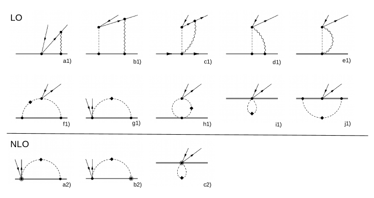
Figure 1: Diagrams contributing to the matching between $\chi$PT and ${/\pi}$EFT at $\mathcal{O}(\epsilon_{\chi}^{0})$ (upper panel) and $\mathcal{O}(\epsilon_{\chi})$ (lower panel). Single, double, wavy, and dashed lines denote, respectively, leptons, nucleons, photons, and pions. Dots refer to interactions from the lowest-order chiral Lagrangians ${\cal L}_{\pi}^{p^{2}}$ and ${\cal L}_{\pi N}^{p}$, while diamonds represent insertions of ${\cal L}_{\pi}^{e^{2}p^{0}}$. Circled dots denote interactions from the NLO chiral Lagrangian ${\cal L}_{\pi N}^{p^{2}}$.

Matching at $\mathcal{O}(\alpha)$ and $O(\alpha\epsilon_{\chi})$ – The diagrams contributing to the matching between $\chi$PT and ${/\pi}$EFT at $\mathcal{O}(\epsilon_{\chi}^{0})$ and $\mathcal{O}(\epsilon_{\chi})$ are shown in Fig. 1. The result of this matching for the leading vector and axial operators is given by

$$g_{V/A} = g_{V/A}^{(0)}\left[1+\sum_{n=2}^{\infty}\Delta_{V/A,\chi}^{(n)}+\frac{\alpha}{2\pi}\sum_{n=0}^{\infty}\Delta^{(n)}_{V/A,\mathrm{em}}\right.$$ (6)

$$\left.+\left(\frac{m_{u}-m_{d}}{\Lambda_{\chi}}\right)^{n_{V/A}}\sum_{n=0}^{\infty}\Delta^{(n)}_{V/A,\delta m}\right]\,,$$

where $g_{V}^{(0)}=1$, $\Delta^{(n)}_{\chi,{\rm em},\delta m}\sim O(\epsilon_{\chi}^{n})$, and $n_{A}=1$, $n_{V}=2$ Behrends and Sirlin (1960); Ademollo and Gatto (1964). Explicit calculation gives $\Delta^{(0),(1)}_{A,\delta m}=0$ and we do not consider the tiny effect of $\Delta^{(0)}_{V,\delta m}\neq 0$. Concerning the chiral corrections in the isospin limit, $\Delta_{V,\chi}^{(n)}$ vanish due to conservation of the vector current, while $\Delta_{A,\chi}^{(n)}$ have been calculated up to $n=4$ in Refs. Bernard et al. (1992); Kambor and Mojzis (1999); Bernard and Meißner (2006), and can for our purposes be absorbed into a definition of $g_{A}$ in the isospin limit, which we denote by $g_{A}^{\rm QCD}$.

To $O(\alpha\epsilon_{\chi}^{0})$ we consider the diagrams in Fig. 1, upper panel. Diagram $(a1)$ appears in the same form in both EFTs, and thus does not contribute to the matching. An explicit calculation shows that the $\mathcal{O}(\epsilon_{/\pi}^{0})$ term of diagrams $(b1)$ and $(d1)$ and $(c1)$ and $(e1)$ cancels, leaving $\mathcal{O}(\epsilon_{/\pi})$ corrections discussed below. Diagrams $(g1)$ and $(j1)$ vanish exactly at $\mathcal{O}(\epsilon_{\chi}^{0})$, while $(f1)$, $(h1)$, $(i1)$ contribute to the vector operator only to be cancelled by corrections to the nucleon wavefunction renormalization (WFR) at $q=0$. As a consequence, $g_{V}$ does not receive loop corrections in the matching between $\chi$PT and ${/\pi}$EFT, instead picking up contributions only from local operators of $\mathcal{O}(e^{2}p)$ so that $\Delta^{(0)}_{V,\rm em}=\hat{C}_{V}$. By contrast, the axial operator is modified through diagram $(i1)$, the WFR, and local operators of $O(e^{2}p)$, leading to

$$\Delta^{(0)}_{A,\rm em}=Z_{\pi}\left[\frac{1+3g^{(0)2}_{A}}{2}\left(\log\frac{\mu^{2}}{m_{\pi}^{2}}-1\right)-g_{A}^{(0)2}\right]+\hat{C}_{A}(\mu)~{}.$$ (7)

We provide in the Appendix the explicit dependence of $\hat{C}_{V,A}$ on the LECs of $\mathcal{O}(e^{2}p)$. Here we note that as written, $\hat{C}_{V,A}$ contain information about short-distance physics and in particular large logarithms connecting the weak scale to the hadronic scale Czarnecki et al. (2004) and finite terms that have been calculated via dispersive methods Seng et al. (2018, 2019); Czarnecki et al. (2019); Shiells et al. (2021).

A similar analysis applies to the NLO amplitude, for which we report a few representative diagrams in the lower panel of Fig. 1. At $q=0$, all diagrams contributing to the vector operator are cancelled by the WFR, resulting in $\Delta^{(1)}_{V,\rm em}=0$. We are left with a correction to $g_{A}$

$$\Delta^{(1)}_{A,\rm em}=Z_{\pi}\,4\pi m_{\pi}\left[c_{4}-c_{3}+\frac{3}{8m_{N}}+\frac{9}{16m_{N}}g_{A}^{(0)2}\right]\,,$$ (8)

dominated by the LECs $c_{3,4}$ from ${\cal L}_{\pi N}^{p^{2}}$ that contribute via topology (a2).

Matching at $\mathcal{O}(\alpha\epsilon_{/\pi})$ — Through our final matching step, we identify additional isospin breaking terms to the LECs of the pion-less Lagrangian. Specifically, the pion loops with the vector current coupling to two pions (topology $(f1)$) induce an isospin-breaking correction to the weak magnetism term. In terms of the physical nucleon magnetic moments, $\mu_{n/p}$ (themselves containing electromagnetic shifts), we find

$$\mu_{\rm weak}-(\mu_{p}-\mu_{n})=-\frac{\alpha Z_{\pi}}{2\pi}\frac{g_{A}^{2}m_{N}\pi}{m_{\pi}}\,.$$ (9)

which is not captured in experimental analyses thus far. Finally, the pion-$\gamma$ box $(b1)$ induces the tensor coupling

$$c_{T}=\frac{\alpha}{2\pi}\frac{g_{A}m_{N}\pi}{3m_{\pi}}\,.$$ (10)

We discuss the numerical implications of these results below.

Connection to previous literature — Recent approaches using current algebra and dispersion techniques Hayen (2021); Gorchtein and Seng (2021) evaluated axial contributions as originating from vertex corrections, in which the virtual photon is emitted and absorbed by the hadronic line, and $\gamma W$ box, in which the virtual photon is exchanged between the hadronic and electron lines. The latter was found to be largely consistent with the vector contribution using experimental data of the polarized Bjorken sum rule Hayen (2021) and additional nucleon scattering data Gorchtein and Seng (2021), as such including inelastic contributions without explicit calculation. The vertex corrections, on the other hand, have only been calculated in limiting scenarios. Following the notation of Ref. Hayen (2021), the a priori non-zero contribution depends on a three-point function

$$\mathcal{D}_{\gamma} =\int\frac{d^{4}k}{k^{2}}\int d^{4}ye^{i\bar{q}y}\int d^{4}xe^{ikx}$$

$$\times\langle p_{f}|T\left\{\partial_{\mu}J^{\mu}_{W}(y)J^{\lambda}_{\gamma}(x)J_{\lambda}^{\gamma}(0)\right\}|p_{i}\rangle\,,$$ (11)

where $\gamma(W)$ denotes electromagnetic (weak) currents, and $T\{\ldots\}$ the time-ordered product. In the chiral limit the divergence of the weak axial current vanishes ($\partial_{\mu}A^{\mu}\propto m_{\pi}\rightarrow 0$), while the vector current is conserved to higher order corrections in $\alpha$ and $m_{d}-m_{u}$. Ref. Hayen (2021) only considered the asymptotic and elastic contributions to Eq. (11), i.e. inserting a complete set of states in between every current and retaining only the nucleon. Assuming isospin symmetry then leads to a vanishing contribution for the three-point function Hayen (2021). Recognizing diagrams $i1,j1,a2,\ldots$ in Fig. 1 to correspond to an explicit treatment of these vertex corrections, the results presented here expand upon the simplified approach of Ref. Hayen (2021) to find much larger than anticipated isospin-breaking corrections.

Numerical impact — We now estimate the numerical impact of the various corrections, starting with our main new finding, i.e., the electromagnetic shift to $\lambda=g_{A}/g_{V}$. Including BSM contributions, the relation between the experimentally extracted $\lambda$ and the (isosymmetric) QCD axial charge is given by Bhattacharya et al. (2012)

$$\lambda=g_{A}^{\mathrm{QCD}}\Big{(}1+\delta^{(\lambda)}_{\mathrm{RC}}-2\mathrm{Re}(\epsilon_{R})\Big{)}~{},$$ (12)

where $\epsilon_{R}\sim(246\,\mathrm{GeV}/\Lambda_{\mathrm{BSM}})^{2}$ is a BSM right-handed current contribution appearing at an energy scale $\Lambda_{\mathrm{BSM}}$ Bhattacharya et al. (2012); Alioli et al. (2017). To the order we are working the radiative correction is

$$\delta^{(\lambda)}_{\mathrm{RC}}=\frac{\alpha}{2\pi}\left(\Delta^{(0)}_{A,\rm em}+\Delta^{(1)}_{A,\rm em}-\Delta^{(0)}_{V\rm em}\right)~{}.$$ (13)

For the numerical evaluation of the loop contributions to $\Delta^{(0),(1)}_{A,\rm em}$ we use $Z_{\pi}=0.81$ (obtained from the physical pion mass difference and $F_{\pi}=92.4$ MeV) and the average nucleon mass $m_{N}=938.9$ MeV. In the loops we set $g_{A}^{(0)}=g_{A}\approx 1.27$ Zyla et al. (2020), as the difference formally contributes to higher chiral order. Existing lattice data indeed indicate that $g_{A}$ has a mild $m_{\pi}$ dependence Chang et al. (2018); Gupta et al. (2018). The NLO LECs $c_{3}$ and $c_{4}$ have been extracted from pion-nucleon scattering Hoferichter et al. (2016); Siemens et al. (2017). They show a sizable dependence on the chiral order at which the fit to $\pi$-$N$ data is carried out, with a big change between NLO and N²LO, stabilizing between N²LO and N³LO. For the corrections we find

$$\Delta^{(0)}_{A-V,\rm em}\in\{2.4,\,5.7\}\,,\ \Delta^{(1)}_{A,\rm em}=\{10.0,14.5,15.9\},$$ (14)

where the range in $\Delta^{(0)}_{A-V,\rm em}$ is obtained by setting $\hat{C}_{A}(\mu)-\hat{C}_{V}=0$ and varying $\mu$ between $0.5$ and $1$ GeV, while the three values of $\Delta^{(1)}_{A,\rm em}$ are obtained by using $c_{3,4}$ extracted to NLO, N²LO, and N³LO Siemens et al. (2017). While the NLO correction is somewhat larger than the LO one, we stress that we do not know the full LO correction because we have set the counter term contribution $\hat{C}_{A}-\hat{C}_{V}$ to zero. In addition, in an EFT without explicit $\Delta$ degrees of freedom, $c_{3}$ and $c_{4}$ are dominated by $\Delta$ contributions and thus anomalously large. Combining the corrections, we estimate a correction to $\lambda$ at the percent level,

$$\delta^{(\lambda)}_{\mathrm{RC}}\in\{1.4,\,2.6\}\cdot 10^{-2}\,.$$ (15)

This shift has no impact on the current first-row CKM discrepancy because the most accurate determination of $\lambda$ is at present obtained from experiments, where these corrections are automatically included. The correction does have a big impact when comparing with first-principles lattice QCD computations of neutron $\beta$ decay. Present lattice calculations of $g_{A}$ work in the isospin limit without QED, but Eq. (15) shows these results cannot be directly compared to the experimentally extracted value of $g_{A}$ without subtracting the newly identified isospin-breaking radiative corrections in this Letter.

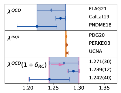
Figure 2: Overview of the required shift to lattice QCD determinations of $g_{A}$ and comparison with current experimental determination of $\lambda$. The bottom panel shows the shift and increased uncertainty in magenta with corrected values. The keys in the figure are FLAG21 Aoki et al. (2021), CalLat19 Walker-Loud et al. (2020), PNDME18 Gupta et al. (2018), PDG21 Zyla et al. (2020), PERKEO3 Märkisch et al. (2019), UCNA Brown et al. (2018).

In Fig. 2 we show the significance of the correction $\delta^{(\lambda)}_{\mathrm{RC}}$ in comparing lattice QCD calculations with the state-of-the-art experimental determination of $\lambda$. Compared to the most precise individual lattice calculation Walker-Loud et al. (2020), our radiative corrections corresponds to a 2.7$\sigma$ shift and a more modest $\sim 1\sigma$ shift in the conservative FLAG’21 average Aoki et al. (2021). $\delta^{(\lambda)}_{\mathrm{RC}}$ generally improves the agreement between lattice QCD and experimental determination of $\lambda$ and is essential if one wishes to obtain robust ranges (or constraints) on right-handed currents. For example, assuming existing central values and an increased lattice-QCD precision, the neglect of radiative corrections ($\delta^{(\lambda)}_{\mathrm{RC}}$) would wrongfully point to BSM physics at $\mathcal{O}(1\,\mathrm{TeV})$.

Isospin-breaking corrections to the weak magnetism do translate into explicit spectral changes (see the appendix for the full differential decay rate). Relative corrections of $\mathcal{O}(10^{-4})$ occur in the SM predictions of both $a$, the $\beta$-$\nu$ angular correlation, and $A$, the $\beta$-asymmetry. These are comparable to anticipated experimental precision in the coming decade within the context of CKM unitarity tests Cirigliano et al. (2019). Even larger relative changes ($\mathcal{O}(0.1\%)$) can occur due to cancellations in the leading-order SM prediction, such as in nuclear mirror systems used in complementary $|V_{ud}|$ determinations Naviliat-Cuncic and Severijns (2009). An extension of this effort to nuclear systems is deemed crucial and fits within rejuvenated superallowed efforts Gorchtein (2019); Hardy and Towner (2020). On the other hand, the induced tensor coupling $c_{T}$ produces a shift to the Fierz term and the neutrino-asymmetry parameter $B$ at the level of $10^{-5}$, negligible in light of the expected experimental accuracies.

Conclusions and outlook — By using a systematic effective field theory approach we have identified and computed novel radiative corrections to neutron $\beta$-decay. The largest correction, at the percent level, can be understood as a QED correction to the nucleon axial charge. While this does not impact the extraction of ${\rm V}_{ud}$ from experiments, it has important consequences for the potential of $\beta$-decay experiments to constrain BSM right-handed currents when comparing the measured value of $\lambda=g_{A}/g_{V}$ to the first-principles calculation of the same quantity with lattice QCD. In addition, we have identified changes in the neutron differential decay rate, in particular a shift in the $\beta$-$\nu$ angular correlation and the $\beta$-asymmetry, that are relevant for next-generation experiments.

The new shift in the nucleon axial charge depends upon non-analytic contributions associated with pion loops as well as analytic short-distance corrections parameterized by LECs. The LECs that lead to the largest part of the correction ($c_{3}$ and $c_{4}$) are precisely extracted from pion-nucleon scattering data, but others are presently unknown leading to a sizable uncertainty in our results. Lattice QCD can compute the hadronic $n\rightarrow p$ amplitude in the presence of QED Carrasco et al. (2015); Giusti et al. (2018), which enables a determination of the unknown LECs. There are subtleties that must be addressed related to gauge invariance and the non-factorizable contributions to the renormalization of the four-fermion operator Di Carlo et al. (2019). ${\rm QED}_{\rm M}$ Endres et al. (2016), in which the photon is given a non-zero mass, may simplify the identification of the matrix element of interest by increasing the energy gap to the excited state contamination.

Looking beyond neutron decay, it is very possible that similar-sized corrections affect nuclear $\beta$-decay. The computations in this Letter provide the first step towards a full EFT treatment of radiative corrections to the multi-nucleon level. Given the interest in these low-energy precision tests of the Standard Model and the existing deviations from first-row CKM unitarity, it is imperative to accurately determine these radiative corrections in order to make full use of the anticipated precision of upcoming experiments.

I Appendix

Effective Lagrangians and power counting — We start from two-flavor QCD in presence of external sources

$${\cal L} = {\cal L}_{\rm QCD}-\ \bar{q}_{R}({s+ip})q_{L}\ -\ \bar{q}_{L}({s-ip})q_{R}$$ (16)

$$+ \bar{q}_{L}\gamma^{\mu}{l_{\mu}}q_{L}\ +\ \bar{q}_{R}\gamma^{\mu}{r_{\mu}}q_{R}$$

where $q^{T}=(u,d)$ and $s(x),p(x),l_{\mu}(x),r_{\mu}(x)$ can be written in terms of quark mass, Standard Model gauge fields, and external classical fields $\bar{s},\bar{p},\bar{l}_{\mu},\bar{r}_{\mu}$ as follows

$$\chi \equiv B_{0}(s+ip)=B_{0}(m_{q}+\bar{s}+i\bar{p})$$ (17a)

$$l_{\mu} = -eQ_{L}^{EM}A_{\mu}\,+\,Q_{L}^{W}J_{\mu}^{\rm lept}\,+\,Q_{L}^{W\dagger}J_{\mu}^{\rm{lept}\dagger}\,+\,\bar{l}_{\mu}\qquad\ \$$ (17b)

$$r_{\mu} = -eQ_{R}^{EM}A_{\mu}\,+\,\bar{r}_{\mu}~{}.$$ (17c)

Here $B_{0}$ is a constant with dimension of mass, $m_{q}$ is the quark mass matrix, $Q_{L}^{EM}=Q_{R}^{EM}=\mathrm{diag}(q_{u},q_{d})$ (with $q_{u}=2/3,q_{d}=-1/3$), $Q_{L}^{W}=-2\sqrt{2}G_{F}V_{ud}\,\tau^{+}$, and $J_{\mu}^{\rm lept}=\bar{e}_{L}\gamma_{\mu}\nu_{eL}$. The Lagrangian in (16) is invariant under local $G=SU(2)_{L}\times SU(2)_{R}\times U(1)_{V}$ transformations

$$q_{L}\to L(x)e^{\alpha_{V}(x)}q_{L}~{},\quad q_{R}\to R(x)e^{\alpha_{V}(x)}q_{R}~{},$$ (18)

with $L,R\in SU(2)_{L,R}$, provided $Q_{L,R}^{EM}$ and $Q_{L}^{W}$ transform as “spurions” under the chiral group $Q_{L}^{EM,W}\to LQ_{L}^{EM,W}L^{\dagger}$ and $Q_{R}^{EM}\to RQ_{R}^{EM}R^{\dagger}$, and that $\bar{l}_{\mu}$ and $\bar{r}_{\mu}$ transform as gauge fields under $G$. This implies

$$\chi \to R\chi L^{\dagger}$$ (19a)

$$l_{\mu} \to Ll_{\mu}L^{\dagger}+iL\partial_{\mu}L^{\dagger}+\partial_{\mu}\alpha_{V}$$ (19b)

$$r_{\mu} \to Rr_{\mu}R^{\dagger}+iR\partial_{\mu}R^{\dagger}+\partial_{\mu}\alpha_{V}~{}.$$ (19c)

Note that the external sources can be decomposed in $SU(2)$ singlet and non-singlet components as follows: $l_{\mu}=l_{\mu}^{ns}+l_{\mu}^{s}$, $r_{\mu}=r_{\mu}^{ns}+r_{\mu}^{s}$.

To construct the effective chiral Lagrangians, one introduces the nucleon and pion fields as follows Coleman et al. (1969); Callan et al. (1969),

$$N=\left(\begin{array}[]{c}p\\ n\end{array}\right),\ U=u^{2}=e^{i\Pi/(F)},\ \Pi=\left(\begin{array}[]{cc}\pi^{0}&\sqrt{2}\pi^{+}\\ \sqrt{2}\pi^{-}&-\pi^{0}\end{array}\right)$$ (20)

and $F\sim F_{\pi}=92.4$ MeV. These fields transform under the chiral group as follows

$$u \to LuK^{\dagger}(u)=K(u)uR^{\dagger}$$ (21a)

$$U \to LUR^{\dagger}$$ (21b)

$$N \to e^{3i\alpha_{V}}K(u)N$$ (21c)

where $K(u)$ is a pion-dependent $SU(2)_{V}$ transformation.

To construct chiral invariant Lagrangians, it is very useful to use chiral-covariant derivatives

$$D_{\mu}U \equiv \partial_{\mu}U-il_{\mu}U+iUr_{\mu}\to L(D_{\mu}U)R^{\dagger}$$ (22a)

$$\nabla_{\mu}N \equiv \left(\partial_{\mu}+\Gamma_{\mu}-i\frac{3(l_{\mu}^{s}+r_{\mu}^{s})}{2}\right)N\to K(\nabla_{\mu}N)\quad\quad\$$ (22b)

$$\Gamma_{\mu} = \frac{1}{2}\left[u(\partial_{\mu}-ir^{ns}_{\mu})u^{\dagger}+u^{\dagger}(\partial_{\mu}-il^{ns}_{\mu})u\right]$$ (22c)

$$\to K(u)\Gamma_{\mu}K(u)^{\dagger}+K(u)\partial_{\mu}K(u)^{\dagger}~{}.$$

It is also very useful to use combinations of fields that transform homogeneously with $K(u)$:

$$u_{\mu} = i\ \left[u(\partial_{\mu}-ir_{\mu})u^{\dagger}-u^{\dagger}(\partial_{\mu}-il_{\mu})u\right]$$ (23a)

$$\to K(u)u_{\mu}K(u)^{\dagger}$$

$$\chi_{\pm} = u^{\dagger}\chi u^{\dagger}\pm u\chi^{\dagger}u\to K(u)\chi_{\pm}K(u)^{\dagger}$$ (23b)

$${\cal Q}_{L}^{EM,W} = u^{\dagger}Q_{L}^{EM,W}u\to K(u){\cal Q}_{L}^{EM,W}K(u)^{\dagger}$$ (23c)

$${\cal Q}_{R}^{EM} = uQ_{R}^{EM}u^{\dagger}\to K(u){\cal Q}_{R}^{EM}K(u)^{\dagger}$$ (23d)

Finally, in the literature one often finds the combinations of charge building blocks with definite parity

$${\cal Q}_{\pm}\equiv\frac{1}{2}\left({\cal Q}_{L}\pm{\cal Q}_{R}\right)~{}.$$ (24)

The standard $\chi$PT power counting assumes that external momenta and meson masses are comparable ($q_{\rm ext}\sim m_{\pi}$). Including charged lepton masses one assumes $p\sim q_{\rm ext}\sim m_{\mu}\sim m_{\pi}\ll\Lambda_{\chi}\sim 4\pi F_{\pi}\sim m_{N}$. Given this, one makes the following assignments:

$$\partial\sim p~{},\quad\chi_{\pm}\sim B_{0}m_{q}\sim m_{\pi}^{2}\sim p^{2}~{}.\quad l_{\mu},r_{\mu}\sim p~{},$$ (25)

with the latter identification implying $e\sim p$ and $G_{F}\sim p$ (though we will never go beyond one insertion of $G_{F}$ and two insertions of the electromagnetic coupling $e$). The above scalings allow us to assign chiral dimension to each lagrangian vertex in a straightforward way.

The pion Lagrangian has the usual expansion in even chiral powers:

$${\cal L}_{\pi} = {\cal L}_{\pi}^{(2)}+{\cal L}_{\pi}^{(4)}+...$$ (26a)

$${\cal L}_{\pi}^{(2)} = {\cal L}_{\pi}^{p^{2}}+{\cal L}_{\pi}^{e^{2}p^{0}}$$ (26b)

$$= \frac{F^{2}}{4}\langle u_{\mu}u^{\mu}+\chi_{+}\rangle+e^{2}Z_{\pi}F^{4}\langle{\cal Q}_{L}^{EM}{\cal Q}_{R}^{EM}\rangle,\qquad$$

which leads to the identification

$$m_{\pi^{\pm}}^{2}-m_{\pi^{0}}^{2}=2e^{2}F_{\pi}^{2}Z_{\pi}~{}.$$ (27)

The gauge-kinetic leptonic Lagrangian has chiral dimension $n=1$:

$${\cal L}_{\rm lept}=\bar{e}\left(i\not{\partial}+e\not{A}-m_{e}\right)e+\bar{\nu}i\not{\partial}\nu~{}.$$ (28)

To the order we work, we need to include the following purely leptonic counter-term Knecht et al. (2000)

$${\cal L}_{\rm lept}^{CT}=e^{2}X_{6}\ \bar{e}\left(i\not{\partial}+e\not{A}\right)e~{}.$$ (29)

The pion-nucleon Lagrangian has both odd and even chiral powers, starting at $n=1$:

$${\cal L}_{\pi N} = {\cal L}_{\pi N}^{(1)}+{\cal L}_{\pi N}^{(2)}+{\cal L}_{\pi N}^{(3)}+...$$ (30a)

$${\cal L}_{\pi N}^{(1)} = {\cal L}_{\pi N}^{p}=\bar{N}_{v}iv\cdot\nabla N_{v}+g_{A}\bar{N}_{v}S\cdot uN_{v}$$ (30b)

$${\cal L}_{\pi N}^{(2)} = {\cal L}_{\pi N}^{p^{2}}+{\cal L}_{\pi N}^{e^{2}p^{0}}$$ (30c)

$${\cal L}_{\pi N}^{(3)} = {\cal L}_{\pi N}^{p^{3}}+{\cal L}_{\pi N}^{e^{2}p}+{\cal L}_{\pi N\ell}^{e^{2}p}$$ (30d)

where in the nucleon rest-frame $v^{\mu}=(1,\bf 0)$ and $S^{\mu}=(0,\boldsymbol{\sigma}/2)$. We have displayed explicitly here only the leading order Lagrangians and we will report below the appropriate higher order terms as needed. All these effective Lagrangian are know in the literature, see for example Ref. Gasser et al. (2002), except for ${\cal L}_{\pi N\ell}^{e^{2}p}$, which is needed to reabsorb divergences from loops that involve virtual baryons, pions, leptons, and photons. We report here only the terms that play a significant role in our analysis.

The one-loop diagrams with virtual nucleons, pions, and photons generate divergences which are absorbed by counterterms in the ${\cal L}_{\pi N}^{e^{2}p}$ Lagrangian. When constructing the baryon electromagnetic Lagrangian, it has been common practice in the literature Meißner and Steininger (1998); Muller and Meißner (1999); Gasser et al. (2002) to use charge spurions corresponding to the nucleon charge matrix $\bar{Q}=diag(1,0)$. Now $\bar{Q}$ differs from the quark charge matrix only in its $SU(2)$ singlet component: therefore the two objects have the same transformation properties under the chiral group and this procedure is justified. In what follows we indicate all the chiral building blocks built from the nucleon charge matrix with a bar. A minimal version of ${\cal L}_{\pi N}^{e^{2}p}$ was constructed in Ref. Gasser et al. (2002)

$${\cal L}_{\pi N}^{e^{2}p}=e^{2}\sum_{i=1,12}\ g_{i}\ \bar{N}_{v}\,O_{i}^{e^{2}p}\,N_{v}~{},$$ (31)

Only four operators contribute to neutron decay at tree level,

$$O_{1}^{e^{2}p} = \langle{\cal\bar{Q}}_{+}^{2}-{\cal\bar{Q}}_{-}^{2}\rangle\,S\cdot u$$ (32a)

$$O_{2}^{e^{2}p} = \langle{\cal\bar{Q}}_{+}\rangle^{2}\,S\cdot u$$ (32b)

$$O_{9}^{e^{2}p} = \frac{i}{2}[{\cal\bar{Q}}_{+},v\cdot c^{+}]+{\rm h.c.}$$ (32c)

$$O_{11}^{e^{2}p} = \frac{i}{2}[{\cal\bar{Q}}_{+},S\cdot c^{-}]~{},$$ (32d)

with

$$c_{\mu}^{\pm}=-\frac{i}{2}\left(u[l_{\mu},\bar{Q}]u^{\dagger}\pm u^{\dagger}[r_{\mu},\bar{Q}]u\right)~{}.$$ (33)

As standard practice in $\chi$PT, the divergences are subtracted as follows Gasser and Leutwyler (1984):

$$g_{i} = \eta_{i}\ \lambda(\mu)+g_{i}^{r}(\mu)~{},$$

$$\lambda(\mu) = \frac{\mu^{d-4}}{(4\pi)^{2}}\left(\frac{1}{d-4}-\frac{1}{2}\left(-\gamma+\log 4\pi+1\right)\right).$$ (34)

We use the same subtraction scheme for all LECs. The coefficients $\eta_{i}$ can be found in Table 5 of Ref. Gasser et al. (2002). We checked that the $g_{i}$ couplings absorb correctly the divergences of diagrams without virtual leptons, thus providing a consistency check on our calculation.

The one-loop diagrams with virtual nucleons, pions, photons, and charged leptons generate divergences which are absorbed by counterterms in the new ${\cal L}_{\pi N\ell}^{e^{2}p}$ Lagrangian. These are the analogue of the operators introduced in the meson sector in Ref. Knecht et al. (2000), that contribute to (semi)leptonic meson decays to $O(e^{2}p^{2})$. We find five structures, of which only the first three contribute to neutron decay at tree level

$${\cal L}_{\pi N\ell}^{e^{2}p}=e^{2}\sum_{i=1,5}\ \tilde{X}_{i}\,\tilde{O}_{i}~{},$$ (35)

where

$$\tilde{O}_{1} = \bar{e}\gamma_{\alpha}\nu_{L}\ \bar{N}_{v}v^{\alpha}{\cal Q}_{L}^{W}N_{v}$$ (36a)

$$\tilde{O}_{2} = \bar{e}\gamma_{\alpha}\nu_{L}\ \bar{N}_{v}v^{\alpha}[{\cal Q}_{L}^{W},{\cal\bar{Q}}_{R}^{EM}]N_{v}$$ (36b)

$$\tilde{O}_{3} = \bar{e}\gamma_{\alpha}\nu_{L}\ \bar{N}_{v}S^{\alpha}[{\cal Q}_{L}^{W},{\cal\bar{Q}}_{R}^{EM}]N_{v}$$ (36c)

$$\tilde{O}_{4} = \bar{e}\gamma_{\alpha}\nu_{L}\ \bar{N}_{v}v^{\alpha}\langle{\cal Q}_{L}^{W}{\cal\bar{Q}}_{R}^{EM}\rangle N_{v}$$ (36d)

$$\tilde{O}_{5} = \bar{e}\gamma_{\alpha}\nu_{L}\ \bar{N}_{v}S^{\alpha}\langle{\cal Q}_{L}^{W}{\cal\bar{Q}}_{R}^{EM}\rangle N_{v}~{}.$$ (36e)

The couplings $\tilde{X}_{i}$ are dimensionless (note that ${\cal Q}_{W}$ carries dimension via the $G_{F}$ factor).

To compute the neutron decay amplitude to $O(G_{F}\alpha\epsilon_{\chi})$ we must consider one-loop diagrams with insertions of ${\cal L}_{\pi N}^{p^{2}}$, for which (in the notation of Ref. Bernard et al. (1995)) we use

$$\mathcal{L}^{p^{2}}_{\pi N} = \bar{N}\Bigg{[}\frac{1}{2m_{N}}\left((v\cdot\mathcal{D})^{2}-\mathcal{D}^{2}\right)-i\frac{g_{A}}{2m_{N}}\left\{S\cdot\mathcal{D},v\cdot u\right\}+c_{1}\textrm{Tr}(\chi_{+})+\left(c_{2}-\frac{g^{2}_{A}}{8m_{N}}\right)(v\cdot u)^{2}$$ (37)

$$+c_{3}u\cdot u+\left(c_{4}+\frac{1}{4m_{N}}\right)\left[S^{\mu},S^{\nu}\right]u_{\mu}u_{\nu}+c_{5}\tilde{\chi}_{+}-\frac{i}{4m_{N}}\left[S^{\mu},S^{\nu}\right]\left((1+\kappa_{1})f^{+}_{\mu\nu}+\frac{1}{2}(\kappa_{0}-\kappa_{1})\textrm{Tr}\left(f^{+}_{\mu\nu}\right)\right)\Bigg{]}N.\qquad$$

Given these Lagrangians, Weinberg’s power counting argument Weinberg (1979, 1990, 1991) implies that connected diagrams scale as ${\cal A}\sim p^{\nu}$ with

$$\nu=2L+1+\sum_{n=2,4,...}(n-2)N_{n}^{M}+\sum_{m=1,2,...}(m-1)N_{m}^{F}$$ (38)

where $L$ is the number of loops and $N_{n}^{M}$ ($N_{m}^{F}$) is the number of mesonic (fermionic) vertices with chiral dimension $n$ ($m$). In deriving this formula, pion propagators are counted as $p^{-2}$ and baryon / lepton propagators are counted as $p^{-1}$.

Using this power counting one sees that the amplitude for neutron decay can be organized as follows

$${\cal A} = {\cal A}^{(1)}+{\cal A}^{(2)}+{\cal A}^{(3)}+{\cal A}^{(4)}+...$$ (39a)

$${\cal A}^{(1)} = {\cal A}^{G_{F}p^{0}}$$ (39b)

$${\cal A}^{(2)} = {\cal A}^{G_{F}p}$$ (39c)

$${\cal A}^{(3)} = {\cal A}^{G_{F}p^{2}}+{\cal A}^{e^{2}G_{F}p^{0}}$$ (39d)

$${\cal A}^{(4)} = {\cal A}^{G_{F}p^{3}}+{\cal A}^{e^{2}G_{F}p}$$

$$...$$

We are interested in computing the leading and next-to-leading electromagnatic corrections to the neutron decay, which appear at chiral order $n=3$ and $n=4$, respectively. Using Eq. (38) one can easily identify the tree-level and one-loop diagrams that contribute to a given order, up to ${\cal A}^{(4)}$:

• The amplitude ${\cal A}^{(1)}$ is given by a tree-level diagram with insertion of the weak vertices from ${\cal L}_{\pi N}^{(1)}$.

• The amplitude ${\cal A}^{(2)}$ is obtained by tree-level graphs with one insertion of ${\cal L}_{\pi N}^{(2)}$ and any number of insertions from ${\cal L}_{\pi N}^{(1)}$ and ${\cal L}_{\pi}^{(2)}$. It contributes to neutron decay at order $G_{F}\epsilon_{\rm recoil}$.

• The amplitude ${\cal A}^{(3)}$ is given by tree-level graphs with one insertion of ${\cal L}_{\pi N}^{(3)}$ and any number of insertions from ${\cal L}_{\pi N}^{(1)}$ and ${\cal L}_{\pi}^{(2)}$; and by one-loop diagrams with vertices from ${\cal L}_{\pi N}^{(1)}$ and ${\cal L}_{\pi}^{(2)}$. In Fig.  1 (upper panel) we show all one-loop topologies contributing up to $O(e^{2}G_{F}p^{0})$, These involve virtual pions, virtual photons, and virtual charged leptons.

• The amplitude ${\cal A}^{(4)}$ is given by tree-level graphs with one insertion of ${\cal L}_{\pi N}^{(4)}$ and any number of insertions from ${\cal L}_{\pi N}^{(1)}$ and ${\cal L}_{\pi}^{(2)}$; and by one-loop diagrams with one vertex from ${\cal L}_{\pi N}^{(2)}$ and any number of vertices from ${\cal L}_{\pi N}^{(1)}$ and ${\cal L}_{\pi}^{(2)}$. Note that tree level graphs with insertion of ${\cal L}_{\pi N}^{(e^{2}p^{2})}$ do not contribute. In Fig.  1 (lower panel) we show representative one-loop diagrams contributing up to $O(e^{2}G_{F}p)$, These involve virtual pions, virtual photons, and virtual charged leptons.

The counterterm contributions to the amplitude at $O(e^{2}G_{F}p^{0})$ are captured by the combinations $\hat{C}_{V/A}$ (see Eq. (7)) as follows:

$$\hat{C}_{A} = 8\pi^{2}\left[-\frac{X_{6}}{2}+\frac{1}{g_{A}^{(0)}}\left[\tilde{X}_{3}+\left(g_{1}+g_{2}+\frac{g_{11}}{2}\right)\right]\right]\ \ \$$

$$\hat{C}_{V} = 8\pi^{2}\left[-\frac{X_{6}}{2}+2\left(\tilde{X}_{1}-\tilde{X}_{2}\right)+g_{9}\right]~{}.$$ (40)

Neutron decay rate — We now present the neutron differential decay rate up-to-and-including $\mathcal{O}(G_{F}\epsilon_{\mathrm{recoil}}$, $\mathcal{O}(G_{F}\alpha)$, $\mathcal{O}(G_{F}\alpha\epsilon_{\chi})$, and $\mathcal{O}(G_{F}\alpha\epsilon_{{/\pi}})$ corrections. We follow Refs. Ando et al. (2004); Gudkov et al. (2006); Bhattacharya et al. (2012) and write

$$\frac{d\Gamma}{dE_{e}d\Omega_{e}d\Omega_{\nu}}=\frac{(G_{F}V_{ud})^{2}}{(2\pi)^{5}}(1+3\lambda^{2})w(E_{e})D(E_{e},\vec{p}_{e},\vec{p}_{\nu},\vec{\sigma}_{n})\,,$$ (41)

where $\vec{\sigma}_{n}$ denotes the neutron polarization and $\lambda=g_{A}/g_{V}$. The spectrum of the electron is described by

$$w=|\vec{p}_{e}|E_{e}(E_{0}-E_{e})^{2}F(E_{e})\left(1+\frac{\alpha}{2\pi}\delta^{(1)}_{\alpha}(E_{e})\right)\,,$$ (42)

where $E_{0}=(m_{n}^{2}-m_{p}^{2}+m_{e}^{2})/(2m_{n})$ is the maximal electron energy, and $F(E_{e})$ is the Fermi function for an electron in the field of the final-state proton. The radiative correction $\delta^{(1)}_{\alpha}$ is discussed below. The function $D$ can be parametrized as

$$D = 1+c_{0}+c_{1}\frac{E_{e}}{m_{N}}+\frac{m_{e}}{E_{e}}\bar{b}+\bar{a}\frac{\vec{p}_{e}\cdot\vec{p}_{\nu}}{E_{e}E_{\nu}}+\bar{A}\frac{\vec{\sigma}\cdot\vec{p}_{e}}{E_{e}}$$ (43)

$$+\bar{B}\frac{\vec{\sigma}\cdot\vec{p}_{\nu}}{E_{\nu}}+\bar{C}_{aa}\left(\frac{\vec{p}_{e}\cdot\vec{p}_{\nu}}{E_{e}E_{\nu}}\right)^{2}$$

$$+\bar{C}_{aA}\frac{\vec{p}_{e}\cdot\vec{p}_{\nu}}{E_{e}E_{\nu}}\frac{\vec{\sigma}\cdot\vec{p}_{e}}{E_{e}}+\bar{C}_{aB}\frac{\vec{p}_{e}\cdot\vec{p}_{\nu}}{E_{e}E_{\nu}}\frac{\vec{\sigma}\cdot\vec{p}_{\nu}}{E_{\nu}}\,.$$

The various coefficients can be further decomposed through Gudkov et al. (2006); Bhattacharya et al. (2012)

$$\bar{a} = \left(a_{\mathrm{LO}}+c_{0}^{(a)}+c_{1}^{(a)}\frac{E_{e}}{m_{N}}\right)\left(1+\frac{\alpha}{2\pi}\delta_{\alpha}^{(2)}(E_{e})\right)\,,$$

$$\bar{A} = \left(A_{\mathrm{LO}}+c_{0}^{(A)}+c_{1}^{(A)}\frac{E_{e}}{m_{N}}\right)\left(1+\frac{\alpha}{2\pi}\delta_{\alpha}^{(2)}(E_{e})\right),$$

$$\bar{B} = B_{\mathrm{LO}}+c_{0}^{(B)}+c_{1}^{(B)}\frac{E_{e}}{m_{N}}+\frac{m_{e}}{E_{e}}b_{\nu}\,,$$

$$\bar{C}_{aa} = c_{1}^{(aa)}\frac{E_{e}}{m_{N}}\,,$$

$$\bar{C}_{aA} = c_{1}^{(aA)}\frac{E_{e}}{m_{N}}\,,$$

$$\bar{C}_{aB} = c_{0}^{(aB)}+c_{1}^{(aB)}\frac{E_{e}}{m_{N}}\,.$$ (44)

The LO coefficients are well known and given by

$$a_{\mathrm{LO}} = \frac{1-\lambda^{2}}{1+3\lambda^{2}}\,,$$

$$A_{\mathrm{LO}} = \frac{2\lambda-2\lambda^{2}}{1+3\lambda^{2}}\,,$$

$$B_{\mathrm{LO}} = \frac{2\lambda+2\lambda^{2}}{1+3\lambda^{2}}\,.$$ (45)

We write the remaining coefficients in terms of $\bar{\mu}_{V}=\mu_{p}-\mu_{n}-\frac{\alpha Z_{\pi}}{2\pi}\frac{g_{A}^{2}m_{N}\pi}{m_{\pi}}$ and $c_{T}=\frac{\alpha}{2\pi}\frac{g_{A}m_{N}\pi}{3m_{\pi}}$

$$\bar{b} = -\frac{m_{e}}{m_{N}}\frac{1+2\lambda(\bar{\mu}_{V}+3c_{T})+\lambda^{2}}{1+3\lambda^{2}}\,,$$

$$c_{0} = -\frac{E_{0}}{m_{N}}\frac{2\lambda(\lambda+\bar{\mu}_{V})}{1+3\lambda^{2}}\,,$$

$$c_{1} = \frac{3+4\lambda\bar{\mu}_{V}+9\lambda^{2}}{1+3\lambda^{2}}\,,$$

$$c^{(a)}_{0} = \frac{E_{0}}{m_{N}}\frac{2\lambda(\lambda+\bar{\mu}_{V})}{1+3\lambda^{2}}\,,$$

$$c^{(a)}_{1} = -\frac{4\lambda(3\lambda+\bar{\mu}_{V})}{1+3\lambda^{2}}\,,$$

$$c^{(A)}_{0} = \frac{E_{0}}{m_{N}}\frac{(\lambda-1)(\lambda+\bar{\mu}_{V})}{1+3\lambda^{2}}\,,$$

$$c^{(A)}_{1} = \frac{\lambda(7-5\lambda)+\bar{\mu}_{V}(1-3\lambda)}{1+3\lambda^{2}}\,,$$

$$c^{(B)}_{0} = -\frac{E_{0}}{m_{N}}\frac{2\lambda(\lambda+\bar{\mu}_{V})}{1+3\lambda^{2}}\,,$$

$$c^{(B)}_{1} = \frac{\lambda(7+5\lambda)+\bar{\mu}_{V}(1+3\lambda)}{1+3\lambda^{2}}\,,$$

$$b_{\nu} = -\frac{m_{e}}{m_{N}}\frac{(1+\lambda)(\lambda+\bar{\mu}_{V})+2c_{T}(1+2\lambda)}{1+3\lambda^{2}}\,,$$

$$c^{(aa)}_{1} = -\frac{3(1-\lambda^{2})}{1+3\lambda^{2}}\,,$$

$$c^{(aA)}_{1} = \frac{(\lambda-1)(5\lambda+\bar{\mu}_{V})}{1+3\lambda^{2}}\,,$$

$$c^{(aB)}_{0} = \frac{E_{0}}{m_{N}}\frac{(1+\lambda)(\lambda+\bar{\mu}_{V})}{1+3\lambda^{2}}\,,$$

$$c^{(aB)}_{1} = -\frac{(1+\lambda)(7\lambda+\bar{\mu}_{V})}{1+3\lambda^{2}}\,.$$ (46)

The explicit expressions for the radiative corrections $\delta^{(1)}_{\alpha}$ and $\delta^{(2)}_{\alpha}$ are given by

$$\delta_{\alpha}^{(1)} = 2\hat{C}_{V}+3\log\frac{\mu}{m_{e}}+\frac{1}{2}$$ (47)

$$+\frac{1+\beta^{2}}{\beta}\,\log\frac{1+\beta}{1-\beta}+\frac{1}{12\beta}\left(\frac{\bar{E}}{E_{e}}\right)^{2}\log\frac{1+\beta}{1-\beta}$$

$$+4\left[\frac{1}{2\beta}\log\frac{1+\beta}{1-\beta}-1\right]\left[\log\frac{2\bar{E}}{m_{e}}-\frac{3}{2}+\frac{\bar{E}}{3E_{e}}\right]$$

$$+\frac{1}{\beta}\left[-4\,{\rm Li}_{2}\left(\frac{2\beta}{1+\beta}\right)-\log^{2}\left(\frac{1+\beta}{1-\beta}\right)\right]\,,$$

$$\delta_{\alpha}^{(2)} = \frac{1-\beta^{2}}{\beta}\,\log\frac{1+\beta}{1-\beta}$$ (48)

$$+\frac{4(1-\beta^{2})}{3\beta^{2}}\frac{\bar{E}}{E_{e}}\left[\frac{1}{2\beta}\log\frac{1+\beta}{1-\beta}-1\right]$$

$$+ \frac{1}{6\beta^{2}}\frac{\bar{E}^{2}}{E_{e}^{2}}\left[\frac{1-\beta^{2}}{2\beta}\log\frac{1+\beta}{1-\beta}-1\right]\,,$$

where $\beta=|\vec{p}_{e}|/E_{e}$ and $\bar{E}=E_{0}-E_{e}$. Our expression for $\delta_{\alpha}^{(1)}$ coincides with the combination of $\delta_{\alpha}^{(1)}+e_{V}^{R}(\mu)$ in Ref. Ando et al. (2004) upon identifying $2\hat{C}_{V}$ with the combination of counterterms $e_{V}-(e_{1}+e_{2})/2$ ] in Ref. Ando et al. (2004). Finally, expressing $\delta_{\alpha}^{(1)}$ in terms of the Sirlin function $g(E_{e},E_{0})$ Sirlin (1967), we find

$$\delta_{\alpha}^{(1)}=2\hat{C}_{V}+\frac{5}{4}+3\log\frac{\mu}{m_{p}}+g(E_{e},E_{0})\,.$$ (49)