a geometrical interpretation of okubo spin group

Abstract.

In this work we define, for the first time, the affine and projective plane over the real Okubo algebra, showing a concrete geometrical interpretation of its Spin group. Okubo algebra is a flexible, composition algebra which is also a not unital division algebra. Even though, Okubo algebra has been known for more than 40 years, we believe that this is the first time the algebra was used for affine and projective geometry. After showing that all axioms of affine geometry are verified, we define a projective plane over Okubo algebra as completion of the affine plane and directly through the use of Veronese coordinates. We then present a bijection between the two constructions. Finally we show a geometric interpretation of $\text{Spin}\left(\mathcal{O}\right)$ as the group of collineations that preserve the axis of the plane.

Msc: 17A20; 17A35; 17A75; 51A35.

1. Introduction and motivations

Unital composition algebras, also known as Hurwitz algebras, are indispensable tools in physics. Even more so the four division Hurwitz algebras that, up to isomorphisms are the Reals $\mathbb{R}$, Complex $\mathbb{C}$, Quaternions $\mathbb{H}$ and Octonions $\mathbb{O}$. All of them share the same propriety of alternativity, i.e.

(1.1) $$\left(x*x\right)*y=x*\left(x*y\right),$$

that, combined with the composition of the norm, i.e.

(1.2) $$n\left(x*y\right)=n\left(x\right)n\left(y\right),$$

allows interesting interplays between physics, geometry and algebra. A wonderful example of those interplays is represented by the Jordan algebras over three by three matrices with coefficient in the Hurwitz algebras, whose rank one idempotents are in bijective correspondence with points on the projective planes[JNW] and whose automorphisms are related to collineations of such plane giving rise to numerous realization of real forms of exceptional Lie groups and algebras [CMCAa].

In this work we will start to analyze the geometrical proprieties of Okubo algebras that are still composition algebras, even though not unital, and enjoy flexibility instead of alternativity, i.e.

(1.3) $$\left(x*y\right)*x=x*\left(y*x\right).$$

The real version of Okubo algebra is even a division algebra and it was studied by Susumo Okubo while he was working on quark and Gellmann matrices in the search of an algebra that had $\text{SU}\left(3\right)$ as automorphisms instead of $\text{G}_{2}$ as in the case of Octonions[Ok95]. Even more interestingly, Okubo discovered that a deformation of the product of this algebra gave back the usual Octonionic product[Ok78, Ok78c, Ok78b].

More recent works [KMRT] with the joint efforts of Elduque and Myung [EM91, EM93, EM90, El15] helped to clarify the context of Okubo algebras that are part of a larger set of algebras called symmetric composition algebra that hosts togheter with Okubo algebras and its split version all the para-Hurwitz algebras, i.e. all the algebras obtained from Hurwitz algebras defining a new product

(1.4) $$x*y=\overline{x}\overline{y}.$$

Later on some algebrical features of Okubo algebra were investigated in order to construct all real form of exceptional Lie groups obtaining a new version of Freudenthal Magic Square[El04, El02]. Nevertheless, a purely geometric construction over Okubo algebra was, to our knowledge, never fully investigated nor even defined. On the other side, in [El18] Elduque gave a description and a definition of the Spin group over Okubo algebras $\text{Spin}\left(\mathcal{O}\right)$ and their triality algebras $\mathfrak{tri}\left(\mathcal{O}\right)$. Here we will give a geometric interpretation of $\text{Spin}\left(\mathcal{O}\right)$, starting from the definition of the Okubic affine plane.

In this work we define for the first time the affine and the projective plane over the real Okubo algebra and investigate some of their geometrical features and interplays. In section $2$ we introduce the real Okubo algebra, while in section $3$ and $4$we introduce the affine and projective plane defining points, lines and elliptic and hyperbolic polarities. In section $5$ we analyze collineations of the plane with a special attention to the triality collineation and, finally, we give a geometric interpretation of $\text{Spin}\left(\mathcal{O}\right)$, which was already defined algebrically in [El15], as the group of collineations that preserve the axis of the plane.

2. Okubo Algebras and Octonions

Following [Ok78] and [EM90], we define the Okubo Algebra $\mathcal{O}$ as the set of three by three Hermitian traceless matrices over the complex numbers $\mathbb{C}$ with the following product

(2.1) $$x*y=\mu\cdot xy+\overline{\mu}\cdot yx-\frac{1}{3}\text{Tr}\left(xy\right),$$

where $\mu=\nicefrac{{1}}{{6}}\left(3+\text{i}\sqrt{3}\right)$ and the juxtaposition is the ordinary associative product between matrices. It is easy to see that the resulting algebra is not unital, not associative and not alternative. Nevertheless, $\mathcal{O}$ is a flexible algebra, i.e.

(2.2) $$x*\left(y*x\right)=\left(x*y\right)*x,$$

which will turn out to be more useful property than alternativity in the definition of the projective plane. Even though the Okubo algebra is not unital, it does have idempotents, i.e. $e*e=e$, such as

(2.3) $$e=\left(\begin{array}[]{ccc}2&0&0\\ 0&-1&0\\ 0&0&-1\end{array}\right),$$

that together with

(2.10) $$\text{i}_{1}=\left(\begin{array}[]{ccc}0&1&0\\ -1&0&0\\ 0&0&0\end{array}\right) ,\,\,\,\,\text{i}_{2}=\left(\begin{array}[]{ccc}0&0&1\\ 0&0&0\\ -1&0&0\end{array}\right),$$

(2.17) $$\text{i}_{3}=\left(\begin{array}[]{ccc}0&0&0\\ 0&0&1\\ 0&-1&0\end{array}\right) ,\,\,\,\,\text{i}_{4}=\left(\begin{array}[]{ccc}0&i&0\\ i&0&0\\ 0&0&0\end{array}\right),$$

(2.27) $$\text{i}_{5}=\left(\begin{array}[]{ccc}0&0&i\\ 0&0&0\\ i&0&0\end{array}\right), \,\,\,\,\,\,\text{i}_{6}=\left(\begin{array}[]{ccc}0&0&0\\ 0&0&i\\ 0&i&0\end{array}\right),\text{i}_{7}=\left(\begin{array}[]{ccc}0&0&0\\ 0&i&0\\ 0&0&-i\end{array}\right),$$

form a basis for $\mathcal{O}$ that has real dimension $8$.

Remark 1.

The Okubo algebra we defined on Hermitian traceless matrices and with real dimension $8$ is called real, while the one defined over $\mathfrak{sl}_{3}\left(\mathbb{C}\right)$ has complex dimension $8$, is not a division algebra and is called complex Okubo algebra. In this work we will only account for the real Okubo algebra, which, as shown in Prop.2 is a division algebra. In a forthcoming paper we study geometryc structure over a complex Okubo algebra.

Let us consider the quadratic form $n$ over Okubo algebra, given by

(2.28) $$n\left(x\right)=\frac{1}{6}\text{Tr}\left(x^{2}\right).$$

It is straightforward to see that this is a norm over $\mathcal{O}$ with respect to which the real Okubo algebra turns to be a composition algebra, i.e.

(2.29) $$n\left(x*y\right) =n\left(x\right)n\left(y\right),$$

(2.30) $$\left\langle x*y,z\right\rangle =\left\langle x,y*z\right\rangle,$$

where $\left\langle\cdot,\cdot\right\rangle$ is the polar form given by

(2.31) $$\left\langle x,y\right\rangle=n\left(x+y\right)-n\left(x\right)-n\left(y\right).$$

Algebras that are flexible and composition such as Okubo are called from [KMRT, Ch. VIII] symmetric composition algebras and enjoy the following notable relation

(2.32) $$x*\left(y*x\right)=\left(x*y\right)*x=n\left(x\right)y.$$

For our purposes it is of paramount importance to notice the following [OM80]

Proposition 2.

The Okubo Algebra is a division algebra

Proof.

Without any loss of generality, let us suppose that $d\neq 0$ is a left divisor of zero, i.e. $d*x=0$, then

$$n\left(d*x\right)=n\left(d\right)n\left(x\right)=0.$$

But, since the algebra is a division algebra and flexible, we have also have

(2.33) $$\left(d*x\right)*d =0=n\left(d\right)x,$$

and therefore $n\left(d\right)=0$, i.e. $\text{Tr}\left(d^{2}\right)=0$. But since the element $d\in\mathcal{O}$ is of the form

$$d=\left(\begin{array}[]{ccc}\xi_{1}&d_{3}&\overline{d}_{2}\\ \overline{d}_{3}&\xi_{2}&d_{1}\\ d_{2}&\overline{d}_{1}&-\xi_{1}-\xi_{2}\end{array}\right),$$

$\text{Tr}\left(d^{2}\right)=0$ is not possible with $\xi_{1},$$\xi_{2}\in\mathbb{R}$ and $\xi_{1},\xi_{2}\neq 0$. ∎

Unfortunately, since $\mathcal{O}$ is not a unital algebra, an element $x$ does not have defined an inverse. Nevertheless, considering the existance of the idempotent $e$, and inspired by the identity

$$x*\left(e*x\right)=\left(x*e\right)*x=n\left(x\right)e,$$

we can define $\left(x\right)_{L}^{-1}=n\left(x\right)^{-1}\left(e*x\right)$ and $\left(x\right)_{R}^{-1}=n\left(x\right)^{-1}\left(x*e\right)$ so that

$$\left(x\right)_{L}^{-1}*x=x*\left(x\right)_{R}^{-1}=e.$$

As an implication of this we have the following

Proposition 3.

Any equation of the kind

(2.34) $$a*x=b,\,\,\text{or}\,\,\,\,x*a=b,$$

has a unique solution which is respectively given by

(2.35) $$x=\frac{1}{n\left(a\right)}b*a,\,\,\,\text{or}\,\,\,\,x=\frac{1}{n\left(a\right)}a*b.$$

Even though, extremely simple the previous proposition has paramount geometrical implications as we show in section 3.

Remark 4.

Since $\mathcal{O}$ is not unital, there is not a canonical involution, as in Hurwitz algebras, of the type $\overline{x}=\left\langle x,\boldsymbol{1}\right\rangle\boldsymbol{1}-x$ such that $n\left(x\right)=x\overline{x}=\overline{x}x$. Nevertheless, the idempotent $e$ gives rise to an automorphism of order two, i.e. an involution, $x\longrightarrow\left\langle x,e\right\rangle e-x$ and an automorphism of order three $x\longrightarrow\tau\left(x\right)=\left\langle x,e\right\rangle e-x*e$, whose geometrical meaning was partially investigated in [El18].

2.1. Deformation to Octonions

The choice of the idempotent $e$ also allows a deformation on the Okubic product that give rise to the usual octonionic product. Indeed, defining a new product over $\mathcal{O}$ by

(2.36) $$x\cdot y=\left(e*x\right)*\left(y*e\right),$$

we obtain that the resulting algebra $\left(\mathcal{O},\cdot,n\right)$ is isomorphic to that of Octonions $\mathbb{O}$, with $e$ as the unit element. Following [El15], it is easy to show that since $e*e=e$ and $n\left(e\right)=1$, for every $x\in\mathcal{O}$ the element $e$ acts as a left and right identity, i.e.

(2.37) $$x\cdot e =e*x*e=n\left(e\right)x=x,$$

(2.38) $$e\cdot x =e*x*e=n\left(e\right)x=x.$$

Moreover, since Okubo algebra is a composition algebra, the same norm $n$ enjoys the following relation

(2.39) $$n\left(x\cdot y\right)=n\left(\left(e*x\right)*\left(y*e\right)\right)=n\left(x\right)n\left(y\right),$$

which means that $\left(\mathcal{O},\cdot,n\right)$ is a unital composition algebra of real dimension $8$ and therefore, as noted by Okubo himself [Ok78, Ok78c, El15], is isomorphic to the algebra of Octonions $\mathbb{O}$.

Remark 5.

Under the previous hypothesis the octonionic identity is $1=e$, while the imaginary units on the Octonions are $\left\{\text{i}_{1},...,\text{i}_{7}\right\}$ in (2.27). Okubo algebras and Octonionic algebras are strictly intertwined: the choice of an idempotent on the Okubo algebra allows the definition of an octonionic product and of a conjugation that can be explicitly given by

(2.40) $$x\cdot y =\left(e*x\right)*\left(y*e\right),$$

(2.41) $$\overline{x} =e*\left(e*\left(e*x\right)\right).$$

2.2. Automorphisms

The first interest of Okubo in its algebra [Ok78, El15] was given by the fact that the group of automorphisms of $\mathcal{O}$ is $\text{Aut}\left(\mathcal{O}\right)\cong SU\left(3\right)$ and its derivations is $\mathfrak{der}\left(\mathcal{O}\right)\cong\mathfrak{su}\left(3\right)$, while in the octonionic case the automorphisms and the derivation led to exceptional group $G_{2\left(-14\right)}$ and $\mathfrak{g}_{2}$. But since $\mathcal{O}$ is a symmetric composition algebra automorphisms of $\mathcal{O}$ it also enjoy the property of preserving the norm. Indeed, let $\varphi$ be an automorphism of $\mathcal{O}$. Then for $x,y\in\mathcal{O}$, since $\varphi\left(x*y\right)=\varphi\left(x\right)*\varphi\left(y\right)$, then we have

(2.42) $$\varphi\left(\left(x*y\right)*x\right) =\varphi\left(n\left(x\right)y\right),$$

but on the other side we also have

(2.43) $$\varphi\left(\left(x*y\right)*x\right) =\left(\varphi\left(x\right)*\varphi\left(y\right)\right)*\varphi\left(x\right)=$$

(2.44) $$=n\left(\varphi\left(x\right)\right)\varphi\left(y\right),$$

and therefore any automorphism of $\mathcal{O}$ preserves the norm, i.e.

(2.45) $$n\left(x\right)=n\left(\varphi\left(x\right)\right),$$

and thus belongs to the orthogonal group $O\left(\mathcal{O}\right)$ and $\left\langle x,y\right\rangle=\left\langle\varphi\left(x\right),\varphi\left(y\right)\right\rangle$ which also means that $\text{tr}\left(xy\right)=\text{tr}\left(\varphi\left(xy\right)\right)$.

3. the affine plane over real okubo algebras

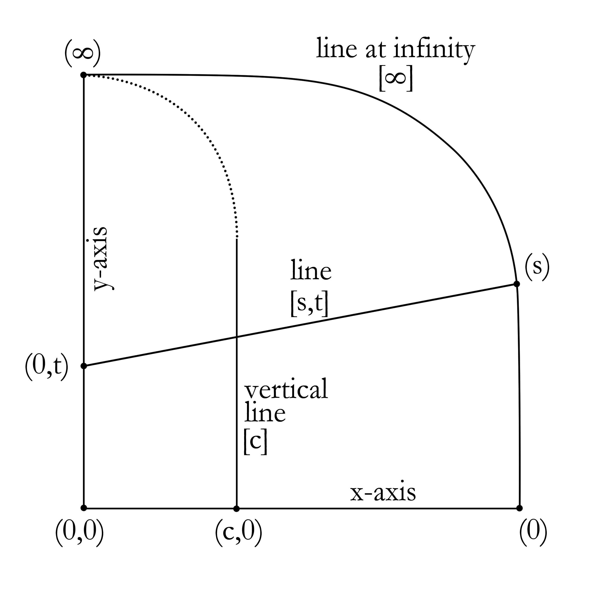
Figure 3.1. Representation of the affine plane: $\left(0,0\right)$ represents the origin, $\left(0\right)$ the point at the infinity on the $x$-axis, $\left(s\right)$ is the point at infinity of the line $\left[s,t\right]$ of slope $s$ while $\left(\infty\right)$ is the point at the infinity on the $y$-axis and of vertical lines $\left[c\right]$.

Following [SBGHLS] we now define Okubic affine plane $\mathscr{A}_{2}\left(\mathcal{O}\right)$ that we will later complete and identify with the projective plane $\mathbb{P}^{2}\mathcal{O}$. A point on the affine plane is identified by two coordinates $\left(x,y\right)$ with $x,y\in\mathcal{O}$, while a line of the affine plane the set $\left\{\left(x,s*x+t\right):x\in\mathcal{O}\right\},$ that we label $\left[s,t\right]$ where $s,t\in\mathcal{O}$ are the slope and the offset respectively. Vertical lines are identified by $\left[c\right]$ and denote the set $\left\{c\right\}\times\mathcal{O}$, where $c\in\mathcal{O}$ represent the intersection with the $x$ axis.

Since $\mathcal{O}$ is a division algebra we then have the following properties:

1. for any two points $\left(x_{1},y_{1}\right)$ and $\left(x_{2},y_{2}\right)$ there is a unique line joining, namely $\left[s,y_{1}-s*x_{1}\right]$, where $s$ is determined by

   $$s*\left(x_{1}-x_{2}\right)=\left(y_{1}-y_{2}\right),$$

   and explicitly found through the use of flexibility

   $$\left(x_{1}-x_{2}\right)*s*\left(x_{1}-x_{2}\right)=\left(x_{1}-x_{2}\right)*\left(y_{1}-y_{2}\right),$$

   that yields to

   $$s=\frac{\left(x_{1}-x_{2}\right)*\left(y_{1}-y_{2}\right)}{n\left(x_{1}-x_{2}\right)},$$

   when $x_{1}\neq x_{2}$ and to the line $\left[x_{1}\right]$ when $x_{1}=x_{2}$.

2. Two lines $\left[s_{1},t_{1}\right]$ and $\left[s_{2},t_{2}\right]$ of different slope, i.e. $s_{1}\neq s_{2}$, have a unique point of intersection $\left\{\left(x,s_{1}*x+t_{1}\right)\right\}$ where

   $$x=\frac{\left(s_{1}-s_{2}\right)*\left(t_{1}-t_{2}\right)}{n\left(s_{1}-s_{2}\right)}.$$

3. Two lines with the same slope are disjoint and therefore are called parallel.

4. For each line $\left[s,t\right]$ and each point $\left(x,y\right)$ there is a unique line which passes through $\left(x,y\right)$ and is parallel to $\left[s,t\right]$, i.e. $\left[s,y-s*x\right]$.

To achieve a completion $\overline{\mathscr{A}_{2}}\left(\mathcal{O}\right)$ of the affine plane, we add another set of coordinates which will represent the points at infinity. Indeed, we add a line at infinity $\left[\infty\right]$, i.e.

$$\left[\infty\right]=\left\{\left(s\right):s\in\mathcal{O}\cup\left\{\infty\right\}\right\},$$

where $\left(s\right)$ identify the end point at infinity of a line with slope $s\in\mathcal{O}\cup\left\{\infty\right\}$. Finally, we define $\left(\infty\right)$ the point at infinity of $\left[\infty\right]$. It is easy to verify that this construction preserves the property of a unique line joining two different points and that two lines intersect at infinity if and only if they are parallel, i.e. have the same slope $\left(s\right)$.

Resuming the whole notation, as in Fig.3.1, we have three set of coordinates that indentify all the points in the completion of the affine plane, i.e. $\left(x,y\right),\left(s\right)$ and $\left(\infty\right)$. The whole affine plane is encompassed by a triangle given by three special points: the origin $\left(0,0\right)$; the 0-point at infinity, i.e. the point $\left(0\right)$ obtained prolonging the $x$ axis to infinity; finally, the $\infty$-point at infinity, i.e. the point $\left(\infty\right)$ obtained prolonging the $y$ axis to infinity. We will call $\triangle$ the set made by those three points, i.e. $\triangle=\left\{\left(0,0\right),\left(0\right),\left(\infty\right)\right\}.$

4. Projective plane over the okubo algebra

We here define the projective plane $\mathbb{P}^{2}\mathcal{O}$ making use of an ad hoc adaptation of the Veronese coordinates introduced in [SBGHLS, CMCAb] for the definition of the Octonionic plane and used in [CMCAa] for the Bioctonionic Rosenfeld plane. After a suitable definition of points and lines of the plane it is straightforward the notion of polarity, which guarantees the projective “spirit” of the construction. Finally, we show that the resulting projective plane is in fact another way of seeing the completion of the affine plane $\overline{\mathscr{A}_{2}}\left(\mathcal{O}\right)$.

4.1. The projective plane

Let $V\cong\mathbb{\mathcal{O}}^{3}\times\mathbb{R}^{3}$ be a real vector space, with elements of the form

$$\left(x_{\nu};\lambda_{\nu}\right)_{\nu}=\left(x_{1},x_{2},x_{3};\lambda_{1},\lambda_{2},\lambda_{3}\right)$$

where $x_{\nu}\in\mathcal{O}$, $\lambda_{\nu}\in\mathbb{R}$ and $\nu=1,2,3$. A vector $w\in V$ is called Okubic Veronese if

(4.1) $$\lambda_{1}x_{1} =x_{2}*x_{3},\,\,\lambda_{2}x_{2}=x_{3}*x_{1},\,\,\lambda_{3}x_{3}=x_{1}*x_{2}$$

(4.2) $$n\left(x_{1}\right) =\lambda_{2}\lambda_{3},\,n\left(x_{2}\right)=\lambda_{3}\lambda_{1},n\left(x_{3}\right)=\lambda_{1}\lambda_{2}.$$

Now we will consider the subspace $H\subset V$ be of Okubo-Veronese vectors. It is straightforward to see that if $w=\left(x_{\nu};\lambda_{\nu}\right)_{\nu}$ is an Okubic Veronese vector then also $\mu w=\mu\left(x_{\nu};\lambda_{\nu}\right)_{\nu}$ is such vector and therefore $\mathbb{R}w\subset H$. We define the Okubic projective plane $\mathbb{P}^{2}\mathcal{O}$ as the geometry having this 1-dimensional subspaces $\mathbb{R}w$ as points, i.e.

(4.3) $$\mathbb{P}^{2}\mathcal{O}=\left\{\mathbb{R}w:w\in H\smallsetminus\left\{0\right\}\right\}.$$

4.2. Lines

The norm on $\mathbb{\mathcal{O}}$ defines the polar form (2.31) that can be extended on $V$ as a symmetric bilinear form

(4.4) $$\beta\left(v,w\right)=\stackrel{{\scriptstyle[}}{{\nu}}=1]{3}{\sum}\left(\left\langle x_{\nu},y_{\nu}\right\rangle+\lambda_{\nu}\eta_{\nu}\right),$$

where $v=\left(x_{\nu};\lambda_{\nu}\right)_{\nu}$ and $w=\left(y_{\nu};\eta_{\nu}\right)_{\nu}$ are Okubo-Veronese vectors in $H\subset V\cong\mathbb{\mathcal{O}}^{3}\times\mathbb{R}^{3}$. Therefore, we define the lines $\ell_{w}$ in the projective plane $\mathbb{P}^{2}\mathcal{O}$ as the orthogonal spaces of a vector $w\in H$, i.e.

(4.5) $$\ell_{w}=w^{\bot}=\left\{z\in V:\beta\left(z,w\right)=0\right\},$$

and, clearly, a point $\mathbb{R}v$ is incident to the line $\ell_{w}$ when $\mathbb{R}v\subseteq$$w^{\bot}$.

Remark 6.

It is worth expliciting how the norm $n$ defined over the symmetric composition algebra $\mathbb{\mathcal{O}}$ is intertwined with the geometry of the plane. This relations is manifest when we consider the quadratic form of the bilinear symmetric form $\beta$, i.e.

(4.6) $$q\left(v\right)\coloneqq\frac{1}{2}\beta\left(v,v\right)=n\left(x_{1}\right)+n\left(x_{2}\right)+n\left(x_{3}\right)+\frac{1}{2}\left(\lambda_{1}^{2}+\lambda_{2}^{2}+\lambda_{3}^{2}\right),$$

4.3. Polarity

Given the previous definitions, it is straightforward to define the standard elliptic polarity $\pi$ that maps points into lines and lines into points through orthogonality, i.e.

(4.7) $$\pi\left(w\right)=w^{\perp},\pi\left(w^{\perp}\right)=w,$$

where $w$ is an Okubo-Veronese vector in $V$.

4.4. Correspondence with the affine plane

The identification of the affine Okubic plane with the projective can be explicited defining the map that sends a point of the affine plane to the projective point in $V\cong\mathbb{\mathcal{O}}^{3}\times\mathbb{R}^{3}$, i.e.

(4.8) $$\left(x,y\right) \mapsto\mathbb{R}\left(x,y,x*y;n\left(y\right),n\left(x\right),1\right),$$

(4.9) $$\left(x\right) \mapsto\mathbb{R}\left(0,0,x;n\left(x\right),1,0\right),$$

(4.10) $$\left(\infty\right) \mapsto\mathbb{R}\left(0,0,0;1,0,0\right).$$

Since the Okubo algebra is a symmetric composition algebra, then the map is well defined. Indeed, from (4.2) we note that

(4.11) $$n\left(x\right)=\lambda_{2},\,\,\,n\left(y\right)=\lambda_{1},$$

and since Okubo is a composition algebra then

(4.12) $$n\left(x*y\right)=n\left(x\right)n\left(y\right).$$

Since Okubo algebra is flexible we also have that (4.1) are satisfied and

$$\lambda_{1}x =y*\left(x*y\right)=n\left(y\right)x,\,\,$$

$$\lambda_{2}y =\left(x*y\right)*x=n\left(x\right)y,$$

$$\lambda_{3}\left(x*y\right) =x*y,$$

and therefore $\mathbb{R}\left(x,y,x*y;n\left(y\right),n\left(x\right),1\right)$ is a point in the Okubic projective plane. As for the converse, if a point $p$ of coordinates $\left(x_{\nu};\lambda_{\nu}\right)_{\nu}$ is in $\mathbb{P}^{2}\mathcal{O}$ then satisfy (4.2) and has one of the $\lambda_{\nu}$ different from zero. Let us suppose $\lambda_{3}=1$. Then by (4.2) we have that $x_{3}=x_{1}*x_{2}$ and therefore the point $p$ is of form $\mathbb{R}\left(x_{1},x_{2},x_{1}*x_{2};n\left(x_{2}\right),n\left(x_{1}\right),1\right)$ and, therefore, corresponds to $\left(x_{1},x_{2}\right)$ in the affine plane. If $\lambda_{3}=0$ and $\lambda_{2}=1$ then the point is of the form $\mathbb{R}\left(0,0,x;n\left(x\right),1,0\right)$ and therefore corresponds to the affine point $\left(x\right)$, while if $\lambda_{1}=1$ and $\lambda_{3}=\lambda_{2}=0$ then the point is $\mathbb{R}\left(0,0,0;1,0,0\right)$ and therefore corresponds to $\left(\infty\right)$.

The same reasoning shows that the correspondence between affine and projective lines given by

(4.13) $$\left[s,t\right] \mapsto\left(t*s,-t,-s;1,n\left(s\right),n\left(t\right)\right)^{\bot},$$

(4.14) $$\left[c\right] \mapsto\left(-c,0,0;0,1,n\left(c\right)\right)^{\bot},$$

(4.15) $$\left[\infty\right] \mapsto\left(0,0,0;0,0,1\right)^{\bot},$$

is also a bijection.

Finally, we need to verify that the image of a point $\left(x,y\right)$ incident to the line $\left[s,t\right]$ goes into a point of the projective plane, i.e. $\mathbb{R}\left(x,y,x*y;n\left(y\right),n\left(x\right),1\right)$, that is incident to the image of the same projective line, i.e. $\left(t*s,-t,-s;1,n\left(s\right),n\left(t\right)\right)^{\bot}$. By definition, for the image of $\left(x,y\right)$ to be incident to the image of $\left[s,t\right]$, the following condition must be satisfied

(4.16) $$\left\langle t*s,x\right\rangle-\left\langle t,y\right\rangle-\left\langle s,x*y\right\rangle+n\left(y\right)+n\left(s\right)n\left(x\right)+n\left(t\right)=0.$$

Noting that

(4.17) $$\left\langle s*x,t-y\right\rangle=n\left(s*x+t-y\right)-n\left(s*x\right)-n\left(t-y\right),$$

and since (2.30), we then have

(4.18) $$\left\langle s*x,t-y\right\rangle =\left\langle s*x,t\right\rangle-\left\langle s*x,y\right\rangle$$

(4.19) $$=\left\langle t,s*x\right\rangle-\left\langle s,x*y\right\rangle$$

(4.20) $$=\left\langle t*s,x\right\rangle-\left\langle s,x*y\right\rangle,$$

and, tehrefore,

(4.21) $$\left\langle t*s,x\right\rangle-\left\langle s,x*y\right\rangle=n\left(s*x+t-y\right)-n\left(s*x\right)-n\left(t-y\right).$$

Inserting the latter into (4.16) and noting that $n\left(s\right)n\left(x\right)=n\left(s*x\right)$ we then have that (4.16) is equivalent to

(4.22) $$n\left(s*x+t-y\right) =0,$$

and, since we are in a division composition algebra, to the condition $s*x+t-y=0$. This means that the above bijection sends affine points incident to an affine line in projective point incident to the same projective line.

5. Collineations and the Spin group

5.1. Collineations

In analogy to the octonionic case, we are now interested in studying the collineations on the completion of Okubic affine plane that we will define as transformations of the plane that send a line into another line, i.e. $\varphi\left(\left[s,t\right]\right)=\left[s^{\prime},t^{\prime}\right]$ with $s,t,s^{\prime},t^{\prime}\in\mathbb{\mathcal{O}}$.

Obviously the set of collineations forms a group under composition and since the identity is a collineation itself, the group is not void. Moreover, throught the use of the Okubic-Veronese coordinates an order three element of the group can be easily spotted, i.e. the triality collineation [SBGHLS] given by a cyclic permutation of the coordinates

(5.1) $$\widetilde{t}:\left(x_{1},x_{2},x_{3};\lambda_{1},\lambda_{2},\lambda_{3}\right)\longrightarrow\left(x_{2},x_{3},x_{1};\lambda_{2},\lambda_{3},\lambda_{1}\right).$$

Proposition 7.

The triality collineation can be red on the affine plane in the following way:

(5.2) $$\widetilde{t}:\begin{cases}\left(x,y\right)&\longrightarrow\frac{1}{n\left(y\right)}\left(y,x*y\right),\,\,\,y\neq 0\\ \left(x\right)&\longrightarrow\frac{1}{n\left(x\right)}\left(0,x\right),x\neq 0\\ \left(x,0\right)&\longrightarrow\left(x\right),\\ \left(0\right)&\longrightarrow\left(\infty\right),\\ \left(\infty\right)&\longrightarrow\left(0,0\right).\end{cases}$$

In particular it induces a collineation $t\colon\mathscr{A}_{2}\left(\mathcal{O}\right)\rightarrow\mathscr{A}_{2}\left(\mathcal{O}\right)$on the affine plane.

Proof.

If $y\neq 0$, the image of $t\left(x,y\right)$ with through the bijection (4.8) in the projective plane is given by

(5.3) $$\frac{1}{n\left(y\right)}\left(y,x*y\right)\longrightarrow\frac{1}{n\left(y\right)}\left(y,x*y,\frac{y*x*y}{n\left(y\right)};\frac{n\left(x*y\right)}{n\left(y\right)},1,n\left(y\right)\right),$$

and since $y*x*y=n\left(y\right)x$ and $n\left(x*y\right)=n\left(x\right)*n\left(y\right)$, then the image of $t\left(x,y\right)$ is in $\mathbb{R}\left(y,x*y,x;n\left(x\right),1,n\left(y\right)\right)$ which is the image of the triality collineation $\widetilde{t}$ of the projective point $\mathbb{R}\left(x,y,x*y;n\left(y\right),n\left(x\right),1\right)$. With the same procedure we find the other correspondences.

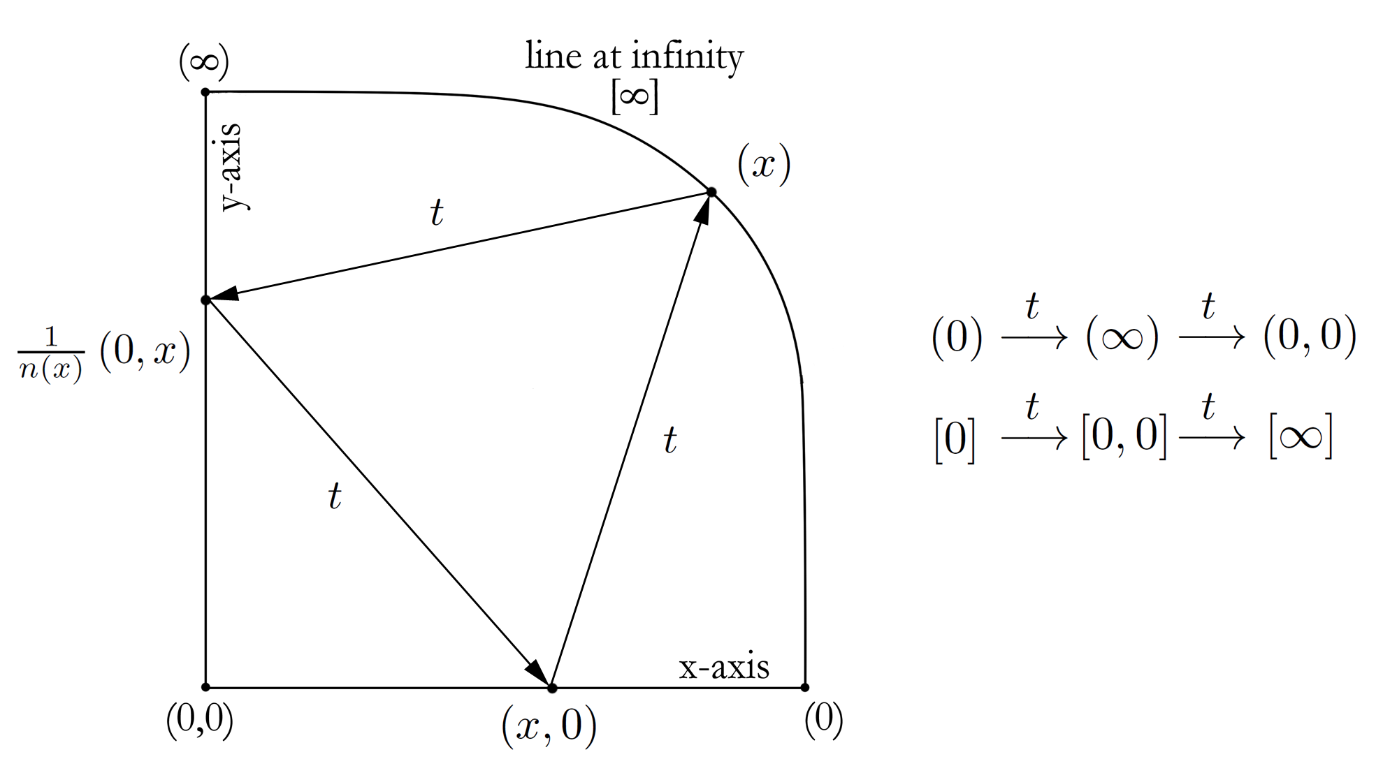
Figure 5.1. Action on the affine plane $\mathscr{A}_{2}\left(\mathcal{O}\right)$ of the triality collineation defined in (5.2).

∎

Remark 8.

As shown in Fig (5.1) the triality collineation $t$ sends the line at infinity $\left[\infty\right]$ into the line $\left[0\right]$, while the $y$ axis $\left[0\right]$ is sent into the $x$ axis $\left[0,0\right]$; finally the $x$ axis $\left[0,0\right]$ is sent into the line at infinity $\left[\infty\right]$. This phenomenon is the dual, of what happens, in the reverse order, for the three points $\left(0,0\right)$,$\left(0\right)$ and $\left(\infty\right)$.

5.2. Recovering the Spin group

While in the previous section we analysed a subgroup of collineations that cyclically permutated the $x-$axis, the $y-$axis and the line at infinity, now we are interested in the subgroup $\Gamma\left(\triangle,\mathbb{\mathcal{O}}\right)$ composed by collineations that fix every point of the triangle $\triangle$, i.e. $\varphi\left(\left(0,0\right)\right)=\left(0,0\right)$, $\varphi\left(\left(0\right)\right)=\left(0\right)$ and $\varphi\left(\left(\infty\right)\right)=\left(\infty\right)$, or, in other words, that fix the $x$ and $y$ axis and, therefore, the line at infinity. This will allow to dive a geometric interpretation of the algebrical definition given in [El15] of the Sping group over the Okubo algebra, i.e. $\text{Spin}\left(\mathcal{O}\right)$.

Proposition 9.

The group $\Gamma\left(\triangle,\mathbb{\mathcal{O}}\right)$ of collineations that fix every point of $\triangle$ are transformations of this form

(5.4) $$\left(x,y\right) \mapsto\left(A\left(x\right),B\left(y\right)\right)$$

(5.5) $$\left(s\right) \mapsto\left(C\left(s\right)\right)$$

(5.6) $$\left(\infty\right) \mapsto\left(\infty\right)$$

where $A,B$ and $C$ are automorphism in respect to the sum over $\mathbb{\mathcal{O}}$ and in respect to multiplication they satisfy

(5.7) $$B\left(s*x\right)=C\left(s\right)*A\left(x\right).$$

Proof.

A collineation that fixes $\left(0,0\right)$, $\left(0\right)$ and $\left(\infty\right)$, it also fixes the $x$-axis and $y$-axis and all lines that are parallel to them. This means that the first coordinate is the image of a function that does not depend on $y$ and the second coordinate is image of a fuction that does not depend of $x$, i.e. $\left(x,y\right)\mapsto\left(A\left(x\right),B\left(y\right)\right)$ and $\left(s\right)\mapsto\left(C\left(s\right)\right)$. Now consider the image of a point on the line $\left[s,t\right]$. The point is of the form $\left(x,s*x+t\right)$ and its image goes to

(5.8) $$\left(x,s*x+t\right)\mapsto\left(A\left(x\right),B\left(s*x+t\right)\right).$$

In order this to be a collineation, the points of $\left[s,t\right]$ must all belong to a line that, setting $x=0$, passes through the points $p_{1}=\left(0,B\left(t\right)\right)$ and $p_{2}=\left(C\left(s\right)\right)$, e.g. $\left[C\left(s\right),B\left(t\right)\right]$. Every line $\left(A\left(x\right),B\left(s*x+t\right)\right)$ passing through $p_{1}$ and $p_{2}$ must satisfy the condition

(5.9) $$B\left(s*x+t\right)=C\left(s\right)*A\left(x\right)+B\left(t\right).$$

Given (5.9), if $B$ is an automorphism with respect to the sum over $\mathbb{\mathcal{O}}$, then $B\left(s*x\right)=C\left(s\right)*A\left(x\right)$. Conversely if $B\left(s*x\right)=C\left(s\right)*A\left(x\right)$ is true than $B\left(s*x+t\right)=B\left(s*x\right)+B\left(t\right)$ and $B$ is an automorphism with respect to the sum. ∎

Let us consider the quadrangle $\boxempty$ given by the points $\left(0,0\right)$, $\left(e,e\right)$, $\left(0\right)$ and $\left(\infty\right)$, that is $\boxempty=\triangle\cup\left\{\left(e,e\right)\right\}$, and consider the collineations that fix the $\boxempty$. Since in addition to the previous case we also have to impose

(5.10) $$\left(e,e\right)\mapsto\left(A\left(e\right),B\left(e\right)\right)=\left(e,e\right),$$

and since $e*e=e$, then $C\left(e\right)=e$ and $A=B=C$. Therefore $A$ is an automorphism of $\mathbb{\mathcal{O}}$. We then have the following

Proposition 10.

Collineations that fix every point of $\boxempty$ are transformations of the type

(5.11) $$\left(x,y\right) \mapsto\left(A\left(x\right),A\left(y\right)\right)$$

(5.12) $$\left(s\right) \mapsto\left(A\left(s\right)\right)$$

(5.13) $$\left(\infty\right) \mapsto\left(\infty\right)$$

where $A$ is an automorphism of $\mathbb{\mathcal{O}}$.

Corollary 11.

The group of collineations $\Gamma\left(\boxempty,\mathcal{O}\right)$ that fix $\left(0,0\right)$, $\left(e,e\right)$, $\left(0\right)$ and $\left(\infty\right)$ is isomorphic to $\text{Aut}\left(\mathcal{O}\right)\cong SL_{3}\left(\mathbb{R}\right)$.

We are now interested in studing the Lie algebras of the previous groups.

Proposition 12.

The Lie algebra $Lie\left(\Gamma\left(\triangle,\mathcal{O}\right)\right)$ of the group of collineation that fixes $\left(0,0\right),\left(0\right)$and $\left(\infty\right)$ is

(5.14) $$\mathfrak{tri}\left(\mathcal{O}\right)=\left\{\left(T_{1},T_{2},T_{3}\right)\in\mathfrak{so}\left(\mathcal{O}\right)^{3}:T_{1}\left(x*y\right)=T_{2}\left(x\right)*y+x*T_{3}\left(y\right)\right\},$$

while the Lie algebra $Lie\left(\Gamma\left(\boxempty,\mathcal{O}\right)\right)$ of the group of collineation that fixes $\left(0,0\right)$, $\left(e,e\right)$, $\left(0\right)$ and $\left(\infty\right)$is

(5.15) $$\mathfrak{der}\left(\mathcal{O}\right)=\left\{A\in\mathfrak{so}\left(\mathcal{O}\right):A\left(x*y\right)=A\left(x\right)*y+x*A\left(y\right)\right\}.$$

Proof.

$\Gamma\left(\triangle,\mathcal{O}\right)$ is a Lie group since it is a closed subgroup of the Lie group of collineations. We will find directly its Lie algebra considering the elements $A,B,C\in\Gamma\left(\triangle,\mathcal{O}\right)$ in a neighbourhood of the identity and writing them as

$$\left(A,B,C\right)\longrightarrow\left(\text{Id}+\epsilon T_{1},\text{Id}+\epsilon T_{2},\text{Id}+\epsilon T_{3}\right)$$

where $T_{1},T_{2},T_{3}\in\mathfrak{so}\left(\mathcal{O}\right)$. Imposing the condition $A\left(x*y\right)=B\left(x\right)*C\left(y\right)$ and then we obtain

(5.16) $$\left(\text{Id}+\epsilon T_{1}\right)\left(x*y\right) =\left(\text{Id}+\epsilon T_{2}\right)\left(x\right)*\left(\text{Id}+\epsilon T_{3}\right)\left(x\right),$$

which, considering $\epsilon^{2}=0$, yields to

(5.17) $$T_{1}\left(x*y\right)=T_{2}\left(x\right)*y+x*T_{3}\left(y\right).$$

As for the second part of the theorem, it suffices to impose $T_{1}=T_{2}=T_{3}$. ∎

Defining the Spin group on Okubo algebras $\text{Spin}\left(\mathcal{O}\right)$, following [El18], as

(5.18) $$\text{Spin}\left(\mathcal{O}\right)=\left\{\left(A,B,C\right)\in O^{+}\left(\mathcal{O}\right)^{3}:A\left(x*y\right)=B\left(x\right)*C\left(y\right)\,\,\,\forall x,y\in\mathcal{O}\right\},$$

where $O^{+}\left(\mathcal{O}\right)$ is the connected component with the identity, we then recover the identification

(5.19) $$\Gamma\left(\triangle,\mathcal{O}\right)\cong \text{Spin}\left(\mathcal{O}\right),$$

(5.20) $$\Gamma\left(\boxempty,\mathcal{O}\right)\cong \text{Aut}\left(\mathcal{O}\right)\cong SU\left(3\right),$$

and, passing to Lie algebras, we obtain

(5.21) $$Lie\left(\Gamma\left(\triangle,\mathcal{O}\right)\right)\cong \mathfrak{tri}\left(\mathcal{O}\right)\cong\mathfrak{su}\left(3\right),$$

(5.22) $$Lie\left(\Gamma\left(\boxempty,\mathcal{O}\right)\right)\cong \mathfrak{der}\left(\mathcal{O}\right)\cong\mathfrak{su}\left(3\right).$$

We then have a perfect analogy with the Octonionic case where the subgroups $\Gamma\left(\triangle,\mathbb{O}\right)$ and $\Gamma\left(\boxempty,\mathbb{O}\right)$ are given by

(5.23) $$\Gamma\left(\triangle,\mathbb{O}\right)\cong \text{Spin}\left(\mathbb{O}\right)\cong\text{Spin}_{8}\left(\mathbb{R}\right),$$

(5.24) $$\Gamma\left(\boxempty,\mathbb{O}\right)\cong \text{Aut}\left(\mathbb{O}\right)\cong\text{G}_{2\left(-14\right)},$$

and the respective Lie algebras are identified with

(5.25) $$Lie\left(\Gamma\left(\triangle,\mathbb{O}\right)\right)\cong \mathfrak{tri}\left(\mathbb{O}\right)\cong\mathfrak{so}\left(\mathbb{\mathbb{O}}\right),$$

(5.26) $$Lie\left(\Gamma\left(\boxempty,\mathbb{O}\right)\right)\cong \mathfrak{der}\left(\mathbb{O}\right)\cong\mathfrak{g}_{2}.$$

6. Conclusions and future developments

In this work we defined for the first time an affine and projective plane over the Okubo algebra. It is mesmerizing and surprising how the analogy between the alternative algebra of Octonions and the flexible Okubo algebra works perfectly with only few changes. Even though, these new affine and projective planes share a numerous proprieties with the classic planes, it is also worth noting that their geometry is far to be completey settled. Jordan algebras over three by three matrices have a perfect analogy with the projective plane over Octonions. It would be then definitely interesting to analyze is an equivalent structure can be realized in the case of Okubo’s algebras. Moreover, interesting geometries arise from the complex Okubo algebra which is not a division algebra but whose divisors of zero enjoy interesting projective proprieties that we plan to cover in our next work.

7. Acknowledgment

$\dagger$Departamento de Matemática,
Universidade do Algarve,
Campus de Gambelas,
8005-139 Faro, Portugal

a55499@ualg.pt.

$\ddagger$Dipartimento di Scienze Matematiche, Informatiche e Fisiche,
Università di Udine,
Udine, 33100, Italy

francesco.zucconi@uniud.it