Degree-Preserving Randomized Response for Graph Neural Networks under Local Differential Privacy

Abstract

Differentially private GNNs (Graph Neural Networks) have been recently studied to provide high accuracy in various tasks on graph data while strongly protecting user privacy. In particular, a recent study proposes an algorithm to protect each user’s feature vector in an attributed graph with LDP (Local Differential Privacy), a strong privacy notion without a trusted third party. However, this algorithm does not protect edges (friendships) in a social graph, hence cannot protect user privacy in unattributed graphs. How to provide strong privacy with high accuracy in unattributed graphs remains open.

In this paper, we propose a novel LDP algorithm called the DPRR (Degree-Preserving Randomized Response) to provide LDP for edges in GNNs. Our DPRR preserves each user’s degree hence a graph structure while providing edge LDP. Technically, our DPRR uses Warner’s RR (Randomized Response) and strategic edge sampling, where each user’s sampling probability is automatically tuned using the Laplacian mechanism to preserve the degree information under edge LDP. We also propose a privacy budget allocation method to make the noise in both Warner’s RR and the Laplacian mechanism small. We focus on graph classification as a task of GNNs and evaluate the DPRR using three social graph datasets. Our experimental results show that the DPRR significantly outperforms three baselines and provides accuracy close to a non-private algorithm in all datasets with a reasonable privacy budget, e.g., $\varepsilon=1$.

I Introduction

Many real-world data are represented as graphs, e.g., social networks, communication networks, and epidemiological networks. GNNs (Graph Neural Networks) [38] have recently attracted much attention because they provide state-of-the-art performance in various tasks on graph data, such as node classification [35], graph classification [58], and community detection [15]. However, the use of graph data raises serious privacy concerns, as it may reveal some sensitive data, such as sensitive edges (i.e., friendships in social graphs) [26].

DP (Differential Privacy) [18] has been widely studied to protect user privacy strongly and is recognized as a gold standard for data privacy. DP provides user privacy against adversaries with any background knowledge when a parameter called the privacy budget $\varepsilon$ is small, e.g., $\varepsilon\leq 1$ or $2$ [36, 27]. According to the underlying architecture, DP can be divided into two types: centralized DP and LDP (Local DP). Centralized DP assumes a centralized model in which a trusted server has the personal data of all users and releases obfuscated versions of statistics or machine learning models. However, this model has a risk that the personal data of all users are leaked from the server by illegal access [39] or internal fraud [14]. In contrast, LDP assumes a local model where a user obfuscates her personal data by herself; i.e., it does not assume a trusted third party. Thus, LDP does not suffer from the data leakage issue explained above, and therefore it has been widely adopted in both the academic field [10, 52, 12, 44] and industry [20, 17].

DP has been recently applied to GNNs [42, 56, 65, 40, 48, 31, 55, 49], and most of them adopt centralized DP. However, they suffer from the data breach issue explained above. Moreover, they cannot be applied to decentralized SNSs (Social Networking Services) [43] such as diaspora* [2] and Mastodon [5]. In decentralized SNSs, the entire graph is distributed across many servers, and each server has only the data of the users who choose it. Because centralized DP algorithms take the entire graph as input, they cannot be applied to the decentralized SNSs. We can also consider fully decentralized SNSs, where a server does not have any edge. For example, we can consider applications where each user sends noisy versions of her friends to the server, which then calculates some graph statistics [29, 28, 61] or generates synthetic graphs [45]. Centralized DP cannot be applied to these applications either.

LDP can be applied to these decentralized SNSs and does not suffer from data leakage. Sajadmanesh and Gatica-Perez [48] apply LDP to each user’s feature vector (attribute values such as age, gender, city, and personal website) in GNNs. They focus on node classification and show that their algorithm provides high classification accuracy with a small privacy budget $\varepsilon$ in LDP, e.g., $\varepsilon=1$.

However, they focus on hiding feature vectors and do not hide edges (friendships). In practice, edges include highly sensitive information, i.e., sensitive friendships. In addition, many social graphs are unattributed graphs [59], which does not include feature vectors and include only node IDs and edges. Unfortunately, the algorithm in [48] cannot be used to protect user privacy in unattributed graphs.

To fill this gap, we focus on LDP for edges in an unattributed graph, i.e., DP in a scenario where each user obfuscates her edges (friend list) by herself. We also focus on graph classification as a task of GNNs (see Section IV-A for details) because a state-of-the-art GNN [58] provides high accuracy for unattributed social graphs in this task. A recent study [66] also shows that a lot of private information can be inferred from the output of GNNs for graph classification. Therefore, LDP algorithms for edges in graph classification are urgently needed.

We first show that Warner’s RR (Randomized Response) [53], which is widely used to provide LDP for edges in applications other than GNNs [29, 28, 61, 45], is insufficient for GNNs. Specifically, the RR flips each 1 (edge) or 0 (no edge) with some probability. The flipping probability is close to $0.5$ when $\varepsilon$ is close to $0$. Consequently, it makes a sparse graph dense and destroys a graph structure. In particular, GNNs use a neighborhood aggregation (or message passing) strategy, which updates each node’s feature vector by aggregating feature vectors of adjacent nodes. In an unattributed graph, a constant value is often used as a feature vector [58, 21], and in this case, the sum of adjacent feature vectors is a degree. Moreover, the degree distribution correlates with the graph type, as shown in our experiments. Thus, each user’s degree is especially important in GNNs. The RR does not preserve the degree information and therefore does not provide high accuracy in GNNs for sparse graphs.

In addition, the RR does not provide high accuracy even in a customized privacy setting (as in Facebook [32]) where some users hide their friend lists and other users reveal their friend lists. We refer to the former users as private users and the latter as non-private users. The RR makes the friend lists of the private users dense. Consequently, it destroys the graph structure and ruins the neighborhood aggregation for non-private users. Thus, the accuracy is hardly increased with an increase in the non-private users, as shown in our experiments. Moreover, the RR has large time and space complexity and is impractical for large-scale graphs; e.g., the memory size is $1$ TB in the Orkut social network [60] with three million users.

To address these issues, we propose a novel LDP algorithm, which we call the DPRR (Degree-Preserving Randomized Response). Our DPRR provides LDP for edges while preserving each user’s degree information. Therefore, it is suitable for the neighborhood aggregation strategy in GNNs. It also works very well in the customized privacy setting – the accuracy is rapidly increased with an increase in non-private users. We show that our DPRR significantly outperforms Warner’s RR, especially in the customized setting. Moreover, we show that the DPRR is much more efficient than the RR in that the DPRR needs much less time for both training and classification and much less memory; e.g., the memory size is about $30$ MB even in the Orkut social network explained above.

We also compare our DPRR with two other private baselines: (i) a local model version of LAPGRAPH (Laplace Mechanism for Graphs) [56] and (ii) an algorithm that discards friend lists of private users and uses a graph composed of only non-private users. We denote the former and latter baselines by LocalLap and NonPriv-Part, respectively. We show that the DPRR significantly outperforms these baselines and provides high accuracy with a reasonable privacy budget, e.g., $\varepsilon=1$.

Our Contributions.  Our contributions are as follows:

• We propose the DPRR for GNNs under LDP for edges. Technically, we use edge sampling [29, 13, 19, 54] after Warner’s RR. In particular, our main technical novelty lies in what we call strategic edge sampling, where each user’s sampling probability is automatically tuned using the Laplacian mechanism to preserve the degree information under edge LDP (see Section IV-C).

• As explained above, the DPRR uses two privacy budgets, one of which is for the Laplacian mechanism while the other is for Warner’s RR. We also propose a privacy budget allocation method to make the noise in both of the mechanisms small and thereby provide high accuracy in GNNs (see Section IV-D).

• We prove that our DPRR approximately preserves the degree information under edge LDP. We also show that our DPRR has much smaller time and space complexity than Warner’s RR (see Sections IV-E and IV-F).

• We focus on graph classification and evaluate our DPRR using three social graph datasets. We show that our DPRR outperforms three private baselines (RR, LocalLap, and NonPriv-Part) in terms of accuracy and the RR in terms of efficiency. We also compare the DPRR with a fully non-private algorithm that does not add any noise for all users, including private users (denoted by NonPriv-Full). For all datasets, we show that our DPRR provides accuracy close to NonPriv-Full (e.g., the difference in the classification accuracy or AUC is smaller than $0.1$ or so) with a reasonable privacy budget, e.g., $\varepsilon=1$ (see Section V).

Our code is available on GitHub [8].

Technical Novelty.  As described above, the technical novelty of our DPRR is two-fold: (i) strategic edge sampling that tunes each user’s sampling probability to preserve the degree information under edge LDP and (ii) privacy budget allocation.

Regarding the first point, Imola et al. [29] propose the ARR (Asymmetric RR) [29], which uses edge sampling after Warner’s RR. Edge sampling has been widely studied to improve the scalability in counting triangles in a graph [13, 19, 54]. The authors in [29] use edge sampling to improve the communication efficiency in triangle counting under LDP. However, they use a sampling probability common to all users and manually set the sampling probability. In this case, the accuracy is not improved by the sampling, because the graph structure remains destroyed. In statistics, random sampling is used to improve efficiency at the expense of accuracy. In fact, edge sampling in [29] decreases the accuracy of triangle counting. In contrast, our DPRR provides higher accuracy than Warner’s RR because it automatically tunes each user’s sampling probability to preserve the degree information.

In other words, our DPRR is different from the ARR [29] (and other existing edge sampling algorithms [13, 19, 54]) in that ours is a strategic sampling algorithm to improve both the accuracy and efficiency in GNNs by preserving the graph structure under edge LDP. The novelty of our strategic sampling technique is not limited to the privacy literature – there are no sampling techniques to improve both the accuracy and efficiency, even in (non-private) triangle counting or graph machine learning, to our knowledge.

In summary, our DPRR is new in that it adopts strategic edge sampling to improve both the accuracy and efficiency. In addition, our privacy budget allocation method that makes the noise in the Laplacian mechanism and Warner’s RR small is also new. We show that they are effective and outperform three baselines in terms of accuracy and efficiency.

II Related Work

DP on GNNs.  In the past year or two, differentially private GNNs [42, 56, 65, 40, 49, 31, 55, 48] (or graph data synthesis [30, 64]) have become a very active research topic. Most of them assume a centralized model [42, 56, 65, 40, 49, 30, 64] where the server has the entire graph (or the exact number of edges in the entire graph [56]). They suffer from the data leakage issue and cannot be applied to decentralized (or fully decentralized) SNSs, as explained in Section I.

Some studies [31, 55] focus on GNNs under LDP in different settings than ours. Specifically, Jin and Chen [31] assume that each user has a graph and apply an LDP algorithm to a graph embedding calculated by each user. In contrast, we consider a totally different scenario, where each user is a node in a graph and the server does not have an edge. Thus, the algorithm in [31] cannot be applied to our setting. Wu et al. [55] assume that each user has a user-item graph and propose a federated GNN learning algorithm for item recommendation. In their work, an edge represents that a user has rated an item. Therefore, their algorithm cannot be applied to our setting where a node and edge represent a user and friendship, respectively. We also note that federated (or collaborative) learning generally requires many interactions between users and the server [34, 51]. In contrast, our DPRR requires only one-round interaction.

Sajadmanesh and Gatica-Perez [48] apply LDP to each user’s feature vectors in an attributed graph. However, they do not hide edges, which are sensitive in a social graph. Consequently, their algorithm cannot be applied to unattributed graphs, where GNNs provide state-of-the-art performance [58].

We also note that LAPGRAPH [56], which assumes the centralized model, can be modified so that it works in the local model setting, as shown in this paper. However, the local model version of LAPGRAPH suffers from low accuracy, as it does not preserve each user’s degree information. In Section V, we show that our DPRR significantly outperforms both Warner’s RR and the local model version of LAPGRAPH.

LDP.  LDP has been widely studied for tabular data where each row corresponds to a user. The main task in this setting is statistical analysis, such as distribution estimation [10, 52, 20] and heavy hitter estimation [12, 44].

LDP has also been used for graph applications other than GNNs, e.g., calculating subgraph counts [29, 28], estimating graph metrics [61], and generating synthetic graphs [45]. Qin et al. [45] propose a synthetic graph data generation technique called LDPGen, which requires two-round interaction between users and the server. However, two-round interaction is impractical for many practical scenarios, as it needs a lot of user effort and synchronization – the server must wait for all users’ responses in each round. This is prohibitively time-consuming when the number of users is large. Thus, we focus on algorithms based on one-round interaction between users and the server. Our DPRR is a one-round algorithm and is much more practical than LDPGen [45].

Qin et al. [45] also propose a one-round algorithm that applies Warner’s RR to each edge. Similarly, the studies in [29, 28, 61] use Warner’s RR to calculate subgraph counts or graph metrics. Since Warner’s RR can also be applied to GNNs, we use it as a baseline. As described in Section I, Warner’s RR makes a sparse graph dense and destroys the graph structure. Consequently, it does not provide high accuracy in GNNs, as shown in our experiments. The study in [41] reduces the number of 1s (edges) in Warner’s RR by sampling without replacement. However, their proof of DP relies on the independence of each edge and is incorrect, as pointed out in [29].

Note that for categorical data of large domain size $k\gg 2$, the RR is outperformed by other LDP algorithms, such as OLH (Optimized Local Hashing) [52], OUE (Optimized Unary Encoding) [52], and HR (Hadamard Response) [10]. However, it is proved in [9] that they are not better than the RR in binary domains ($k=2$). Moreover, we consider a setting where both the input domain and the output range are binary (i.e., “edge” or “no edge”) to make LDP mechanisms applicable to GNNs. In this setting (i.e., when output data are compressed to binary bits), all of the OLH, OUE, and HR are identical to Warner’s RR, as they are symmetric. We also note that applying them to an entire neighbor list ($k=2^{n}$) results in prohibitively large noise, as $k$ is too large. Therefore, Warner’s RR for each bit of the neighbor list has been widely used in graphs [29, 28, 61, 45]. We also focus on Warner’s RR.

III Preliminaries

In this section, we describe some preliminaries needed for this paper. Section III-A defines basic notation. Section III-B reviews LDP on graphs. Section III-C explains GNNs.

III-A Basic Notation

Let $\mathbb{R}$, $\mathbb{R}_{\geq 0}$, $\mathbb{N}$, $\mathbb{Z}_{\geq 0}$ be the sets of real numbers, non-negative real numbers, natural numbers, and non-negative integers, respectively. For $a\in\mathbb{N}$, let $[a]=\{1,2,\cdots,a\}$.

Consider an unattributed social graph with $n\in\mathbb{N}$ nodes (users). Let $\mathcal{G}$ be the set of possible graphs, and $G=(V,E)\in\mathcal{G}$ be a graph with a set of nodes $V=\{v_{1},v_{2},\cdots,v_{n}\}$ and a set of edges $E\subseteq V\times V$. The graph $G$ can be either directed or undirected. In a directed graph, an edge $(v_{i},v_{j})\in E$ represents that user $v_{i}$ follows user $v_{j}$. In an undirected graph, an edge $(v_{i},v_{j})$ represents that $v_{i}$ is a friend with $v_{j}$.

A graph $G$ can be represented as an adjacency matrix $\mathbf{A}=(a_{i,j})\in\{0,1\}^{n\times n}$, where $a_{i,j}=1$ if and only if $(v_{i},v_{j})\in E$. Note that the diagonal elements are always $0$; i.e., $a_{1,1}=\cdots=a_{n,n}=0$. If $G$ is an undirected graph, $\mathbf{A}$ is symmetric. Let $\mathbf{a}_{i}=(a_{i,1},a_{i,2},\cdots,a_{i,n})\in\{0,1\}^{n}$ be the $i$-th row of $\mathbf{A}$. $\mathbf{a}_{i}$ is called the neighbor list [45] of user $v_{i}$. Let $d_{i}\in\mathbb{Z}_{\geq 0}$ be the degree of user $v_{i}$. Note that $d_{i}=||\mathbf{a}_{i}||_{1}$, i.e., the number of 1s in $\mathbf{a}_{i}$. Let $\mathcal{N}(v_{i})$ be the set of nodes adjacent to $v_{i}$, i.e., $v_{j}\in\mathcal{N}(v_{i})$ if and only if $(v_{i},v_{j})\in E$.

We focus on a local privacy model [29, 28, 61, 45], where user $v_{i}$ obfuscates her neighbor list $\mathbf{a}_{i}$ using a local randomizer $\mathcal{R}\hskip 0.28453pt_{i}$ and sends the obfuscated data $\mathcal{R}\hskip 0.28453pt_{i}(\mathbf{a}_{i})$ to a server. Table I shows the basic notation used in this paper.

TABLE I: Basic notation in this paper.

Symbol Description $n$ Number of users. $\mathcal{G}$ Set of possible graphs. $G=(V,E)$ Graph with users $V$ and edges $E$. $v_{i}$ $i$-th user. $\mathbf{A}=(a_{i,j})$ Adjacency matrix. $\mathbf{a}_{i}$ Neighbor list of user $v_{i}$. $d_{i}$ Degree of user $v_{i}$. $\mathcal{N}(v_{i})$ Set of nodes adjacent to user $v_{i}$. $\mathcal{R}\hskip 0.28453pt_{i}$ Local randomizer of user $v_{i}$.

III-B Local Differential Privacy on Graphs

Edge LDP.  The local randomizer $\mathcal{R}\hskip 0.28453pt_{i}$ of user $v_{i}$ adds some noise to her neighbor list $\mathbf{a}_{i}$ to hide her edges. Here, we assume that the server and other users can be honest-but-curious adversaries and can obtain all edges in $G$ other than edges of $v_{i}$ as background knowledge. To strongly protect edges of $v_{i}$ from these adversaries, we use DP as a privacy metric. In graphs, there are two types of DP: node DP and edge DP [46]. Node DP hides one node along with its edges from the adversary. However, many applications in the local privacy model require a user to send her user ID, and we cannot use node DP for these applications. Therefore, we use edge DP in the same way as the previous work on graph LDP [29, 28, 61, 45].

Edge DP hides one edge between any two users from the adversary. Its local privacy model version, called edge LDP [45], is defined as follows:

Definition 1 ($\varepsilon$-edge LDP [45]).

Let $\varepsilon\in\mathbb{R}_{\geq 0}$ and $i\in[n]$. A local randomizer $\mathcal{R}\hskip 0.28453pt_{i}$ of user $v_{i}$ with domain $\{0,1\}^{n}$ provides $\varepsilon$-edge LDP if and only if for any two neighbor lists $\mathbf{a}_{i},\mathbf{a}^{\prime}_{i}\in\{0,1\}^{n}$ that differ in one bit and any $s\in\mathrm{Range}(\mathcal{R}\hskip 0.28453pt_{i})$,

$$\Pr[\mathcal{R}\hskip 0.28453pt_{i}(\mathbf{a}_{i})=s]\leq e^{\varepsilon}\Pr[\mathcal{R}\hskip 0.28453pt_{i}(\mathbf{a}^{\prime}_{i})=s].$$ (1)

For example, the randomized neighbor list in [45] applies Warner’s RR (Randomized Response) [53], which flips 0/1 with probability $\frac{1}{e^{\varepsilon}+1}$, to each bit of $\mathbf{a}_{i}$ (except for $a_{i,i}$). By (1), this randomizer provides $\varepsilon$-edge LDP.

The parameter $\varepsilon$ is called the privacy budget, and the value of $\varepsilon$ is crucial in DP. By (1), the likelihood of $\mathbf{a}_{i}$ is almost the same as that of $\mathbf{a}^{\prime}_{i}$ when $\varepsilon$ is close to $0$. However, they can be very different when $\varepsilon$ is large. For example, it is well known that $\varepsilon\leq 1$ or $2$ is acceptable for many practical scenarios, whereas $\varepsilon\geq 5$ is unsuitable in most scenarios [36, 27]. Based on this, we set $\varepsilon\leq 2$ in our experiments.

Edge LDP can be used to hide each user’s neighbor list $\mathbf{a}_{i}$. For example, in Facebook, user $v_{i}$ can change her setting so that anyone except for server administrators cannot see her neighbor list $\mathbf{a}_{i}$. By using edge LDP with small $\varepsilon$, we can hide $\mathbf{a}_{i}$ even from the server administrators.

Relationship DP.  In an undirected graph, each edge $(v_{i},v_{j})$ is shared by two users $v_{i}$ and $v_{j}$. Thus, both users’ outputs can leak the information about $(v_{i},v_{j})$. Imola et al. [28] define relationship DP to protect each edge during the whole process:

Definition 2 ($\varepsilon$-relationship DP [28]).

Let $\varepsilon\in\mathbb{R}_{\geq 0}$. A tuple of local randomizers $(\mathcal{R}\hskip 0.28453pt_{1},\cdots,\mathcal{R}\hskip 0.28453pt_{n})$ provides $\varepsilon$-relationship DP if and only if for any two undirected graphs $G,G^{\prime}\in\mathcal{G}$ that differ in one edge and any $(s_{1},\ldots,s_{n})\in\mathrm{Range}(\mathcal{R}\hskip 0.28453pt_{1})\times\ldots\times\mathrm{Range}(\mathcal{R}\hskip 0.28453pt_{n})$,

$$\Pr[(\mathcal{R}\hskip 0.28453pt_{1}(\mathbf{a}_{1}),\ldots,\mathcal{R}\hskip 0.28453pt_{n}(\mathbf{a}_{n}))=(s_{1},\ldots,s_{n})]$$

$$\leq e^{\varepsilon}\Pr[(\mathcal{R}\hskip 0.28453pt_{1}(\mathbf{a}^{\prime}_{1}),\ldots,\mathcal{R}\hskip 0.28453pt_{n}(\mathbf{a}^{\prime}_{n}))=(s_{1},\ldots,s_{n})],$$ (2)

where $\mathbf{a}_{i}$ (resp. $\mathbf{a}_{i}^{\prime}$) is the $i$-th row of the adjacency matrix of $G$ (resp. $G^{\prime}$).

Proposition 1 (Edge LDP and relationship DP [28]).

In an undirected graph, if each of local randomizers $\mathcal{R}\hskip 0.28453pt_{1},\ldots,\mathcal{R}\hskip 0.28453pt_{n}$ provides $\varepsilon$-edge LDP, then $(\mathcal{R}\hskip 0.28453pt_{1},\ldots,\mathcal{R}\hskip 0.28453pt_{n})$ provides $2\varepsilon$-relationship DP.

In Proposition 1, relationship DP has the doubling factor in $\varepsilon$ because the presence/absence of one edge $(v_{i},v_{j})$ affects two bits $a_{i,j}$ and $a_{j,i}$ in neighbor lists in an undirected graph.

Note that even if user $v_{i}$ hides her neighbor list $\mathbf{a}_{i}$, her edge with her friend $v_{j}$ will be disclosed when $v_{j}$ releases $\mathbf{a}_{j}$. This is inevitable in social networks based on undirected graphs. For example, in Facebook, user $v_{i}$ can change her setting so that no one can see $\mathbf{a}_{i}$. However, she can also change the setting so that $\mathbf{a}_{i}$ is public. Thus, if user $v_{i}$ hides $\mathbf{a}_{i}$ and her friend $v_{j}$ reveals $\mathbf{a}_{j}$, their edge $(v_{i},v_{j})$ is disclosed. To prevent this, $v_{i}$ needs to ask $v_{j}$ not to reveal $\mathbf{a}_{j}$.

In other words, relationship DP requires some trust assumptions, unlike LDP; i.e., if a user wants to keep all her edges secret, she needs to trust her friends not to reveal their neighbor lists. However, even if her $k\in\mathbb{N}$ friends reveal their neighbor lists, only her $k$ edges will be disclosed. Therefore, the trust assumption of relationship DP is much weaker than that of centralized DP, where the server can leak all edges.

Global Sensitivity.  As explained above, Warner’s RR is one of the simplest approaches to providing edge LDP. Another well-known approach is to use global sensitivity [18]:

Definition 3.

In edge LDP, the global sensitivity $GS_{f}$ of a function $f:\{0,1\}^{n}\rightarrow\mathbb{R}$ is given by

$$GS_{f}=\underset{\mathbf{a}_{i},\mathbf{a}^{\prime}_{i}\in\{0,1\}^{n},\mathbf{a}_{i}\sim\mathbf{a}^{\prime}_{i}}{\max}|f(\mathbf{a}_{i})-f(\mathbf{a}^{\prime}_{i})|,$$

where $\mathbf{a}_{i}\sim\mathbf{a}^{\prime}_{i}$ represents that $\mathbf{a}_{i}$ and $\mathbf{a}^{\prime}_{i}$ differ in one bit.

For $b\in\mathbb{R}_{\geq 0}$, let $\textrm{Lap}(b)$ be the Laplacian noise with mean $0$ and scale $b$. Then, adding the Laplacian noise $\textrm{Lap}(\frac{GS_{f}}{\varepsilon})$ to $f$ provides $\varepsilon$-edge LDP.

III-C Graph Neural Networks

Graph Classification.  We focus on graph classification as a task of GNNs. The goal of graph classification is to predict a label of the entire graph, e.g., type of community, type of online discussion (i.e., subreddit [6]), and music genre users in the graph are interested in.

More specifically, we are given multiple graphs, some of which have a label. Let $\mathcal{G}_{l}=\{G_{1},\cdots,G_{|\mathcal{G}_{l}|}\}\subseteq\mathcal{G}$ be the set of labeled graphs, and $\mathcal{G}_{u}=\{G_{|\mathcal{G}_{l}|+1},\cdots,G_{|\mathcal{G}_{l}|+|\mathcal{G}_{u}|}\}\subseteq\mathcal{G}$ be the set of unlabeled graphs. Graph classification is a task that finds a mapping function $\phi$ that takes a graph $G\in\mathcal{G}$ as input and outputs a label $\phi(G)$. We train a mapping function $\phi$ from labeled graphs $\mathcal{G}_{l}$. Then, we can predict labels for unlabeled graphs using the trained function $\phi$.

The GNN is a machine learning model useful for graph classification. Given a graph $G\in\mathcal{G}$, the GNN calculates a feature vector $h_{G}$ of the entire graph $G$. Then it predicts a label based on $h_{G}$, e.g., by a softmax layer.

Neighborhood Aggregation.  Most GNNs use a neighborhood aggregation (or message passing) strategy, which updates a node feature of each node $v_{i}$ by aggregating node features of adjacent nodes $\mathcal{N}(v_{i})$ and combining them [38, 22]. Specifically, each layer in a GNN has an aggregate function and a combine (or update) function. For $k\in\mathbb{Z}_{\geq 0}$, let $h_{i}^{(k)}$ be a feature vector of $v_{i}$ at the $k$-th layer. Since we focus on an unattributed graph $G$, we create the initial feature vector $h_{i}^{(0)}$ from the graph structure, e.g., a one-hot encoding of the degree of $v_{i}$ or a constant value [58, 21].

At the $k$-th layer, we calculate $h_{i}^{(k)}$ as follows:

$$m_{i}^{(k)} =\textsf{AGGREGATE}^{(k)}(\{h_{j}^{(k-1)}:v_{j}\in\mathcal{N}(v_{i})\})$$ (3)

$$h_{i}^{(k)} =\textsf{COMBINE}^{(k)}(h_{i}^{(k-1)},m_{i}^{(k)}).$$ (4)

$\textsf{AGGREGATE}^{(k)}$ is an aggregate function that takes feature vectors $h_{j}^{(k-1)}$ of adjacent nodes $\mathcal{N}(v_{i})$ as input and outputs a message $m_{i}^{(k)}$ for user $v_{i}$. Examples of $\textsf{AGGREGATE}^{(k)}$ include a sum [58], mean [35, 24], and max [24]. $\textsf{COMBINE}^{(k)}$ is a combine function that takes a feature vector $h_{i}^{(k-1)}$ of $v_{i}$ and the message $m_{i}^{(k)}$ as input and outputs a new feature vector $h_{i}^{(k)}$. Examples of $\textsf{COMBINE}^{(k)}$ include one-layer perceptrons [24] and MLPs (Multi-Layer Perceptrons) [58].

Note that (3) uses the set $\mathcal{N}(v_{i})$ of nodes adjacent to $v_{i}$ and therefore can leak the edge information. Since the algorithm in [48] hides only node features, it reveals edge information in (3) and violates edge LDP. In other words, the algorithm in [48] cannot be used to protect privacy in unattributed graphs.

For graph classification, the GNN outputs a feature vector $h_{G}$ of the entire graph. $h_{G}$ is calculated by aggregating feature vectors $h_{i}^{(K)}$ of the final iteration $K\in\mathbb{N}$ as follows:

$$h_{G} =\textsf{READOUT}(\{h_{i}^{(K)}:v_{i}\in V\}).$$ (5)

READOUT is a readout function, such as a sum [58], mean [58], and hierarchical graph pooling [63].

IV Degree-Preserving Randomized Response

We propose a local randomizer that provides LDP for edges in the original graph while keeping high classification accuracy in GNNs. A simple way to provide LDP for edges is to use Warner’s RR (Randomized Response) [53] to each bit of a neighbor list. However, it suffers from low classification accuracy because the RR makes a sparse graph dense and destroys a graph structure, as explained in Section I. To address this issue, we propose a local randomizer called the DPRR (Degree-Preserving Randomized Response), which provides edge LDP while preserving each user’s degree.

Section IV-A explains a system model assumed in our work. Section IV-B describes the overview of our DPRR. Section IV-C explains our DPRR in detail. Section IV-D proposes a privacy budget allocation method for our DPRR. Section IV-E shows the degree preservation properties of our DPRR. Finally, Section IV-F shows the time and space complexity of our DPRR.

IV-A System Model

Fig. 1 shows a system model in this paper. First, we assume that there are multiple social graphs, some of which have a label. We can consider several practical scenarios for this.

Figure 1: System model. For each graph $G$, users $v_{1},\cdots,v_{n}$ send their noisy neighbor lists $\tilde{\mathbf{a}}_{1},\cdots,\tilde{\mathbf{a}}_{n}$ providing edge LDP. Then, the server calculates a noisy adjacency matrix $\tilde{\mathbf{A}}$ corresponding to $\tilde{\mathbf{a}}_{1},\cdots,\tilde{\mathbf{a}}_{n}$. The server trains the GNN using matrices $\tilde{\mathbf{A}}$ of labeled graphs and predicts a label for each unlabeled graph using its matrix $\tilde{\mathbf{A}}$ and the trained GNN.

For example, some social networks (e.g., Reddit [6]) provide online discussion threads. In this case, each discussion thread can be represented as a graph, where an edge represents that a conversation happens between two users, and a label represents a category (e.g., subreddit) of the thread. The REDDIT-MULTI-5K and REDDIT-BINARY [59] are real datasets in this scenario and are used in our experiments.

For another example, we can consider multiple decentralized SNSs, as described in Section I. Some SNSs may have a topic, such as music, game, food, and business [5, 7, 4]. In this scenario, each SNS corresponds to a graph, and a label represents a topic.

Based on the labeled and unlabeled social graphs, we perform graph classification privately. Specifically, for each graph $G=(V,E)$, each user $v_{i}\in V$ obfuscates her neighbor list $\mathbf{a}_{i}\in\{0,1\}^{n}$ using a local randomizer $\mathcal{R}\hskip 0.28453pt_{i}$ providing $\varepsilon_{i}$-edge LDP and sends her noisy neighbor lists $\tilde{\mathbf{a}}_{i}\in\{0,1\}^{n}$ to a server. Then, the server calculates a noisy adjacency matrix $\tilde{\mathbf{A}}\in\{0,1\}^{n\times n}$ corresponding to $\tilde{\mathbf{a}}_{1},\cdots,\tilde{\mathbf{a}}_{n}$. The server trains the GNN using noisy adjacency matrices $\tilde{\mathbf{A}}$ of labeled graphs. Then, the server predicts a label for each unlabeled graph based on its noisy adjacency matrix $\tilde{\mathbf{A}}$ and the trained GNN.

Note that we consider a personalized setting [33], where each user $v_{i}$ can set her privacy budget $\varepsilon_{i}$. In particular, we consider the following two basic settings:

• Common Setting. In this setting, all users adopt the same privacy budget $\varepsilon$, i.e., $\varepsilon=\varepsilon_{1}=\varepsilon_{2}=\cdots=\varepsilon_{n}$. This is a scenario assumed in most studies on DP. By Proposition 1, a tuple of local randomizers $(\mathcal{R}\hskip 0.28453pt_{1},\ldots,\mathcal{R}\hskip 0.28453pt_{n})$ provides $2\varepsilon$-relationship DP in the common setting when the graph $G$ is undirected.

• Customized Setting. In this setting, some private users adopt a small privacy budget (e.g., $\varepsilon=1$) and other non-private users make their neighbor lists public (i.e., $\varepsilon=\infty$). This is similar to Facebook’s setting. Specifically, in Facebook, each user $v_{i}$ can change her setting so that no one (except for the server) can see $\mathbf{a}_{i}$. User $v_{i}$ can also change her setting so that $\mathbf{a}_{i}$ is public. Our customized setting is stronger than Facebook’s setting in that a private user $v_{i}$ hides $\mathbf{a}_{i}$ even from the server.

Recall that in an undirected graph, even if $v_{i}$ hides her neighbor list $\mathbf{a}_{i}$, her edge with $v_{j}$ can be disclosed when $v_{j}$ makes $\mathbf{a}_{j}$ public. In other words, a tuple of local randomizers $(\mathcal{R}\hskip 0.28453pt_{1},\ldots,\mathcal{R}\hskip 0.28453pt_{n})$ does not provide relationship DP in the customized setting where one or more users are non-private.

However, the customized setting still makes sense because it is a stronger version of Facebook’s setting; i.e., our customized setting hides the neighbor list $\mathbf{a}_{i}$ of the private user $v_{i}$ even from the server. In our customized setting, even if $k\in\mathbb{N}$ friends are non-private, only $k$ edges with them will be disclosed, as described in Section III-B. All edges between private users will be kept secret, even from the server.

In our experiments, we show that our DPRR is effective in both common and customized settings.

IV-B Algorithm Overview

Fig. 3 shows the overview of our DPRR, which takes a neighbor list $\mathbf{a}_{i}\in\{0,1\}^{n}$ of user $v_{i}$ as input and outputs a noisy neighbor list $\tilde{\mathbf{a}}_{i}\in\{0,1\}^{n}$. We also show the details of the RR and edge sampling in Fig. 3.

Figure 2: Overview of the DPRR (Degree-Preserving Randomized Response).

Figure 3: RR and edge sampling.

As shown in Figs. 3 and 3, we use edge sampling after Warner’s RR to avoid a dense noisy graph. For each bit of the neighbor list $\mathbf{a}_{i}$, Warner’s RR outputs 0/1 as is with probability $p\in[0,1]$ and flips 0/1 with probability $1-p$. Then, for each 1 (edge), edge sampling outputs 1 with probability $q_{i}\in[0,1]$ and 0 with probability $1-q_{i}$. Here, the degree information of each user is especially important in GNNs because it represents the number of adjacent nodes in the aggregate step. Thus, we carefully tune the sampling probability $q_{i}$ of each user $v_{i}$ so that the number of 1s in $\tilde{\mathbf{a}}_{i}$ is close to the original degree $d_{i}$ ($=||\mathbf{a}_{i}||_{1}$).

Note that we cannot use $d_{i}$ itself to tune the sampling probability, because $d_{i}$ leaks the information about edges of $v_{i}$. To address this issue, we tune the sampling probability by replacing $d_{i}$ with a private estimate of $d_{i}$ providing edge LDP. Both the RR and the private estimate of $d_{i}$ provide edge LDP. Thus, by the (general) sequential composition [36], the noisy neighbor list $\tilde{\mathbf{a}}_{i}$ is also protected with edge LDP.

Specifically, the DPRR works as follows. We first calculate a degree $d_{i}$ from the neighbor list $\mathbf{a}_{i}$ and add the Laplacian noise to the degree $d_{i}$. Consequently, we obtain a private estimate $d_{i}^{*}\in\mathbb{R}$ of $d_{i}$ with edge LDP. Then, we tune the sampling probability $q_{i}$ using $d_{i}^{*}$ so that the expected number of 1s in $\tilde{\mathbf{a}}_{i}$ is equal to $d_{i}$. Finally, we apply Warner’s RR to $\mathbf{a}_{i}$ and then randomly sample 1s with the sampling probability $q_{i}$. As a result, we obtain the noisy neighbor list $\tilde{\mathbf{a}}_{i}$ whose noisy degree $\tilde{d}_{i}=||\tilde{\mathbf{a}}_{i}||_{1}$ is almost unbiased; i.e., the expectation of $\tilde{d}_{i}$ is almost equal to $d_{i}$. In Section IV-C, we explain the details of the DPRR algorithm.

Note that the DPRR uses two privacy budgets. One is for the Laplacian noise, and the other is for Warner’s RR. In Section IV-D, we propose a privacy budget allocation method so that the variance of the noisy degree $\tilde{d}_{i}$ is small. Since the noisy degree $\tilde{d}_{i}$ is almost unbiased and has a small variance, the noisy neighbor list $\tilde{\mathbf{a}}_{i}$ preserves the degree information of user $v_{i}$. In Section IV-E, we formally prove this property.

IV-C Algorithm Details

Algorithm 1 shows an algorithm for the DPRR. It assigns privacy budgets $\varepsilon_{1},\varepsilon_{2}\in\mathbb{R}_{\geq 0}$ to the Laplacian noise and RR, respectively.

Algorithm 1 Degree-Preserving Randomized Response

0:  neighbor list $\mathbf{a}_{i}\in\{0,1\}^{n}$, $\varepsilon_{1},\varepsilon_{2}\in\mathbb{R}_{\geq 0}$

0:  noisy neighbor list $\tilde{\mathbf{a}}_{i}\in\{0,1\}^{n}$

1:  $d_{i}\leftarrow||\mathbf{a}_{i}||_{1}$

2:  $d_{i}^{*}\leftarrow d_{i}+\textrm{Lap}(\frac{1}{\varepsilon_{1}})$

3:  $p\leftarrow\frac{e^{\varepsilon_{2}}}{e^{\varepsilon_{2}}+1}$

4:  $q_{i}\leftarrow\frac{d_{i}^{*}}{d_{i}^{*}(2p-1)+(n-1)(1-p)}$

5:  $q_{i}\leftarrow\texttt{Proj}(q_{i})$

6:  $\tilde{\mathbf{a}}_{i}\leftarrow\texttt{RR}(\mathbf{a}_{i},p)$

7:  $\tilde{\mathbf{a}}_{i}\leftarrow\texttt{EdgeSampling}(\tilde{\mathbf{a}}_{i},q_{i})$

8:  return  $\tilde{\mathbf{a}}_{i}$

First, we add the Laplacian noise $\textrm{Lap}(\frac{1}{\varepsilon_{1}})$ to the degree $d_{i}$ ($=||\mathbf{a}_{i}||_{1}$) of user $v_{i}$ to obtain a private estimate $d_{i}^{*}$ of $d_{i}$: $d_{i}^{*}=d_{i}+\textrm{Lap}(\frac{1}{\varepsilon_{1}})$ (lines 1-2). Then we tune the sampling probability $q_{i}$ as follows:

$$q_{i}=\frac{d_{i}^{*}}{d_{i}^{*}(2p-1)+(n-1)(1-p)},$$ (6)

where $p=\frac{e^{\varepsilon_{2}}}{e^{\varepsilon_{2}}+1}$ (lines 3-4). $p$ represents the probability that Warner’s RR sends an input value as is; i.e., it flips 0/1 with probability $1-p=\frac{1}{e^{\varepsilon_{2}}+1}$. In Section IV-E, we show that the noisy degree $\tilde{d}_{i}=||\tilde{\mathbf{a}}_{i}||_{1}$ becomes almost unbiased by setting $q_{i}$ by (6).

Note that there is a small probability that $q_{i}$ in (6) is outside of $[0,1]$. Thus, we call the Proj function, which projects $q_{i}$ onto $[0,1]$; i.e., if $q_{i}<0$ (resp. $q_{i}>1$), then we set $q_{i}=0$ (resp. $q_{i}=1$) (line 5).

Next, we apply Warner’s RR to a neighbor list $\mathbf{a}_{i}$ of $v_{i}$. Specifically, we call the RR function, which takes $\mathbf{a}_{i}$ and $p$ as input and outputs a noisy neighbor list $\tilde{\mathbf{a}}_{i}$ by sending each bit as is with probability $p$ (line 6). Finally, we apply edge sampling to $\tilde{\mathbf{a}}_{i}$. Specifically, we call the EdgeSampling function, which randomly samples each 1 (edge) with probability $q_{i}$ (line 7).

In summary, we output $\tilde{\mathbf{a}}_{i}$ by the RR and edge sampling with the following probability:

$$\Pr(\tilde{a}_{i,j}=1)=\begin{cases}pq_{i}&(\text{if }a_{i,j}=1)\\ (1-p)q_{i}&(\text{otherwise}),\end{cases}$$ (7)

where $\tilde{a}_{i,j}\in\{0,1\}$ is the $j$-th element of $\tilde{\mathbf{a}}_{i}$ ($i\neq j$).

Privacy.  Below, we show the privacy property of the DPRR.

Proposition 2.

The DPRR (Algorithm 1) provides $\varepsilon$-edge LDP, where $\varepsilon=\varepsilon_{1}+\varepsilon_{2}$.

The proof is given in Appendix A. Since DP is immune to post-processing [18], the GNN model trained from the noisy adjacency matrix $\tilde{\mathbf{A}}$ provides $(\varepsilon_{1}+\varepsilon_{2})$-edge LDP as well.

IV-D Privacy Budget Allocation

Our DPRR uses two privacy budgets: $\varepsilon_{1}$ for the Laplacian noise and $\varepsilon_{2}$ for the RR. When $\varepsilon_{1}$ is too small, the Laplacian noise becomes too large and causes a large variance of the noisy degree $\tilde{d}_{i}=||\tilde{\mathbf{a}}_{i}||_{1}$. In contrast, when $\varepsilon_{2}$ is too small, the RR adds too much noise to each edge. Below, we propose a method to allocate $\varepsilon_{1}$ and $\varepsilon_{2}$ to avoid these two issues. In a nutshell, our privacy allocation method sets $\varepsilon_{1}$ to guarantee a small variance of $\tilde{d}_{i}$ while keeping a large value of $\varepsilon_{2}$ to make the noise in the RR small.

Specifically, let $n_{max}\in\mathbb{R}_{\geq 0}$ be the maximum number of nodes (users) in all graphs $\mathcal{G}_{l}$ and $\mathcal{G}_{u}$. In Section IV-E, we show that if $\varepsilon_{1}<\sqrt{\frac{8}{n_{max}-1}}$, the Laplacian noise is too large and causes a large variance of $\tilde{d}_{i}$. Taking this into account, our privacy budget allocation method sets $\varepsilon_{1}$ as follows:

$$\textstyle{\varepsilon_{1}=\max\left\{\sqrt{\frac{8}{n_{max}-1}},(1-\alpha)\varepsilon\right\},}$$ (8)

where $\alpha$ is a constant close to $1$ ($\alpha=0.9$ in our experiments).

This setting makes the variance of $\tilde{d}_{i}$ small (i.e., $\varepsilon_{1}\geq\sqrt{\frac{8}{n_{max}-1}}$). It also allows the Laplacian noise to decrease with increase in $\varepsilon$. Moreover, it makes the noise in the RR small (i.e., it makes $\varepsilon_{2}$ large), as $\alpha$ is large. In our experiments, we show that this setting makes the variance of the noisy degree $\tilde{d}_{i}$ small and provides high classification accuracy in GNNs.

IV-E Degree Preservation Property

We now show the degree preservation property of the DPRR. Specifically, we analyze the expectation and variance of the noisy degree $\tilde{d}_{i}=||\tilde{\mathbf{a}}_{i}||_{1}$.

Expectation of the Noisy Degree.  We first analyze the expectation $\mathbb{E}[\tilde{d}_{i}]$ of the noisy degree $\tilde{d}_{i}$ over the randomness in the Laplacian noise, the RR, and the edge sampling. By the law of total expectation, we have

$$\mathbb{E}[\tilde{d}_{i}]=\mathbb{E}[\mathbb{E}[\tilde{d}_{i}|d_{i}^{*}]],$$ (9)

where $d_{i}^{*}$ is a private estimate of $d_{i}$ (see line 2 of Algorithm 1). The original neighbor list $\mathbf{a}_{i}$ has $d_{i}$ 1s and $n-1-d_{i}$ 0s (except for $a_{i,i}$). By (7), the DPRR sends 1 as is with probability $pq_{i}$ and flips 0 to 1 with probability $(1-p)q_{i}$. Thus, we have

$$\mathbb{E}[\tilde{d}_{i}|d_{i}^{*}] =d_{i}pq_{i}+(n-1-d_{i})(1-p)q_{i}$$

$$=(d_{i}(2p-1)+(n-1)(1-p))q_{i}$$

$$=\textstyle{\frac{d_{i}(2p-1)+(n-1)(1-p)}{d_{i}^{*}(2p-1)+(n-1)(1-p)}d_{i}^{*}~{}~{}~{}~{}\text{(by (\ref{eq:q_i}))}}.$$

In practice, real social graphs are sparse, which means that $d_{i},d_{i}^{*}\ll n$ holds for the vast majority of nodes. In addition, $p=\frac{e^{\varepsilon_{2}}}{e^{\varepsilon_{2}}+1}$ is not close to $1$ when $\varepsilon_{2}$ is small, e.g., $p=0.73$ when $\varepsilon_{2}=1$. We are interested in such a value of $p$; otherwise, we cannot provide edge privacy. Thus, we have $d_{i}(2p-1),d_{i}^{*}(2p-1)\ll(n-1)(1-p)$, hence

$$\textstyle{\mathbb{E}[\tilde{d}_{i}|d_{i}^{*}]\approx\frac{(n-1)(1-p)}{(n-1)(1-p)}d_{i}^{*}=d_{i}^{*}.}$$ (10)

By (9) and (10), we have

$$\mathbb{E}[\tilde{d}_{i}]\approx\mathbb{E}[d_{i}^{*}]=d_{i}~{}~{}\text{(as the mean of $\textstyle{\textrm{Lap}(\frac{1}{\varepsilon_{1}})}$ is $0$)},$$ (11)

which means that the noisy degree $\tilde{d}_{i}$ is almost unbiased.

Variance of the Noisy Degree.  Next, we analyze the variance $\mathbb{V}[\tilde{d}_{i}]$ of the noisy degree $\tilde{d}_{i}$. By the law of total variance, we have

$$\mathbb{V}[\tilde{d}_{i}]=\mathbb{E}\left[\mathbb{V}[\tilde{d}_{i}|d_{i}^{*}]\right]+\mathbb{V}\left[\mathbb{E}[\tilde{d}_{i}|d_{i}^{*}]\right].$$ (12)

Recall that the original neighbor list $\mathbf{a}_{i}$ has $d_{i}$ 1s and $n-1-d_{i}$ 0s. By (7), we have

$$\mathbb{V}[\tilde{d}_{i}|d_{i}^{*}]$$

$$=d_{i}pq_{i}(1-pq_{i})+(n-1-d_{i})(1-p)q_{i}(1-(1-p)q_{i})$$

$$\leq\textstyle{\frac{n_{max}-1}{4},}$$ (13)

where the equality holds if and only if $n=n_{max}$, $p=\frac{1}{2}$ and $q_{i}=1$. By (10), the second term of (12) can be written as follows:

$$\textstyle{\mathbb{V}\left[\mathbb{E}[\tilde{d}_{i}|d_{i}^{*}]\right]\approx\mathbb{V}[d_{i}^{*}]=\mathbb{V}[\textrm{Lap}(\frac{1}{\varepsilon_{1}})}]=\frac{2}{\varepsilon_{1}^{2}}.$$ (14)

By (12), (13), and (14), we have

$$\textstyle{\mathbb{V}[\tilde{d}_{i}]\approx\mathbb{E}\left[\mathbb{V}[\tilde{d}_{i}|d_{i}^{*}]\right]+\mathbb{V}\left[d_{i}^{*}\right]\leq\frac{n_{max}-1}{4}+\frac{2}{\varepsilon_{1}^{2}}.}$$ (15)

The first term of (15) is caused by the randomness of the RR, whereas the second term of (15) is caused by the randomness of the Laplacian noise.

If $\varepsilon_{1}<\sqrt{\frac{8}{n_{max}-1}}$, the second term of (15) is larger than the first term of (15); i.e., the Laplacian noise is dominant. Thus, our privacy allocation method sets $\varepsilon_{1}\geq\sqrt{\frac{8}{n_{max}-1}}$ (see (8)). In this case, the variance is bounded as follows: $\mathbb{V}[\tilde{d}_{i}]\leq\frac{n_{max}-1}{2}$.

Summary.  Our DPRR makes the noisy degree $\tilde{d}_{i}=||\tilde{\mathbf{a}}_{i}||_{1}$ almost unbiased by automatically tuning the sampling probability $q_{i}$ by (6). In addition, our privacy allocation method makes the variance of $\tilde{d}_{i}$ small (i.e., $\mathbb{V}[\tilde{d}_{i}]\leq\frac{n_{max}-1}{2}$) by setting $\varepsilon_{1}$ by (8). Consequently, the noisy neighbor list $\tilde{\mathbf{a}}_{i}$ preserves the degree information of user $v_{i}$. We also show this degree-preserving property of the DPRR through experiments.

IV-F Time and Space Complexity

Finally, we show that our DPRR has much smaller time and space complexity than Warner’s RR.

TABLE II: Time and space complexity of three LDP algorithms per graph.

Algorithm Time Time Space Space (Each User) (Server) (Each User) (Server) DPRR $O(n)$ $O(|E|)$ $O(n)$ $O(|E|)$ RR $O(n)$ $O(n^{2})$ $O(n)$ $O(n^{2})$ LocalLap $O(n)$ $O(|E|)$ $O(n)$ $O(|E|)$

Table II shows the time and space complexity of three LDP algorithms: the DPRR, Warner’s RR applied to each bit of the adjacency matrix $\mathbf{A}$, and a local model version of LAPGRAPH [56] (LocalLap). We explain the details of LocalLap in Section V-A. In Table II, we assume that the server runs efficient GNN algorithms whose time complexity is linear in the number of edges, e.g., GIN (Graph Isomorphism Network) [58], GCN (Graph Convolutional Networks) [35], and GraphSAGE (Graph Sample and Aggregate) [24]. Some of the other GNN algorithms are less efficient; see [57] for details.

Table II shows that the time and space complexity on the server side is $O(n^{2})$ in Warner’s RR. This is because the RR makes a graph dense; i.e., $|\tilde{\mathbf{A}}|=O(n^{2})$. In contrast, the DPRR preserves each user’s degree information, and consequently, $|\tilde{\mathbf{A}}|=O(|E|)$, where $|E|$ is the number of edges in the original graph $G$. Thus, the DPRR has the time and space complexity of $O(|E|)$ on the server side. Since $|E|\ll n^{2}$ in practice, the DPRR is much more efficient than the RR.

For example, the Orkut social network [60] includes $3072441$ nodes and $117185083$ edges. The RR needs a memory size of $1$ TB for this graph. In contrast, the memory size of the DPRR is only about $30$ MB, which is much smaller than that of the RR. In our experiments, we also show that the DPRR needs much less time for both training and classification.

LocalLap has the same time and space complexity as the DPRR. In our experiments, we show that our DPRR significantly outperforms LocalLap in terms of accuracy.

Note that each user’s time and space complexity is much smaller than the server’s. Specifically, all of the DPRR, RR, and LocalLap have the time and space complexity of $O(n)$ because the length of each user’s neighbor list is $O(n)$.

TABLE III: Statistics of graph datasets. “#nodes” represents the number of nodes in a single graph.

Dataset #graphs #classes #nodes (max) #nodes (avg) degree (max) degree (avg) REDDIT-MULTI-5K 4999 5 3782 508.5 2011 2.34 REDDIT-BINARY 2000 2 3648 429.6 3062 2.32 Github StarGazers 12725 2 957 113.8 755 4.12

V Experimental Evaluation

Based on the theoretical properties of our DPRR in Sections IV-E and IV-F, we pose the following research questions:

RQ1.

How does our DPRR compare with other private algorithms in terms of accuracy and time complexity?

RQ2.

How accurate is our DPRR compared to a non-private algorithm?

RQ3.

How much does our DPRR preserve each user’s degree information?

We conducted experiments to answer these questions.

V-A Experimental Set-up

Dataset.  We used three unattributed social graph datasets:

• REDDIT-MULTI-5K.  REDDIT-MULTI-5K [59] is a graph dataset in Reddit [6], where each graph represents an online discussion thread. An edge between two nodes represents that a conversation happens between the two users. A label represents the type of subreddit, and there are five subreddits: worldnews, videos, AdviceAnimals, aww, and mildyinteresting.

• REDDIT-BINARY.  REDDIT-BINARY [59] is a social graph dataset in Reddit. The difference from REDDIT-MULTI-5K lies in labels. In REDDIT-BINARY, a label represents a type of community, and there are two types of communities: a question/answer-based community and a discussion-based community.

• Github StarGazers.  Github StarGazers [47] includes a social network of developers who starred popular machine learning and web development repositories until August 2019. A node represents a user, and an edge represents a follower relationship. A label represents the type of repository: machine learning or web.

Table III shows statistics of each graph dataset.

LDP Algorithms.  For comparison, we evaluated the following four private algorithms:

• DPRR.  Our proposed algorithm providing $\varepsilon$-edge LDP, where $\varepsilon=\varepsilon_{1}+\varepsilon_{2}$ (Algorithm 1). As described in Section IV-D, we set $\varepsilon_{1}=\max\left\{\sqrt{\frac{8}{n_{max}-1}},(1-\alpha)\varepsilon\right\}$ and $\varepsilon_{2}=\alpha\varepsilon$, where $n_{max}$ is the maximum number of nodes and $\alpha=0.9$.

• RR.  Warner’s RR for each bit of the neighbor list [29, 28, 61, 45]. It flips each 0/1 with probability $\frac{1}{e^{\varepsilon}+1}$. It provides $\varepsilon$-edge LDP.

• LocalLap.  A local model version of LAPGRAPH [56]. LAPGRAPH is an algorithm providing edge DP in the centralized model. Specifically, LAPGRAPH adds $\textrm{Lap}(\frac{1}{\varepsilon_{1}})$ to the total number of edges in a graph $G$. Then it adds $\textrm{Lap}(\frac{1}{\varepsilon_{2}})$ to each element in the upper-triangular part of $\mathbf{A}$ and selects $T$ largest elements (edges), where $T$ is the noisy number of edges. Finally, it outputs a noisy graph with the selected edges.

  LAPGRAPH cannot be used in the local model, as it needs the total number of edges in $G$ as input. Thus, we modified LAPGRAPH so that each user $v_{i}$ sends a noisy degree $d_{i}^{*}$ ($=d_{i}+\textrm{Lap}(\frac{1}{\varepsilon_{1}})$) to the server and the server calculates the noisy number $T$ of edges as: $T=(\sum_{i=1}^{n}d_{i}^{*})/2$. We call this modified algorithm LocalLap. LocalLap provides $\varepsilon$-edge LDP, where $\varepsilon=\varepsilon_{1}+\varepsilon_{2}$. We set $\varepsilon_{1}=\frac{\varepsilon}{10}$ and $\varepsilon_{2}=\frac{9\varepsilon}{10}$.

• NonPriv-Part.  An algorithm that discards friend lists of private users and uses only friend lists of non-private users. Specifically, it constructs a graph composed of only non-private users and uses it as input to GNN.

Note that NonPriv-Part is an algorithm in the customized setting and cannot be used in the common setting.

We also evaluated NonPriv-Full, a fully non-private algorithm that does not add any noise for all users. Note that NonPriv-Full does not protect privacy for private users, unlike the four private algorithms explained above. The accuracy of private algorithms is high if it is close to that of NonPriv-Full.

Finally, we emphasize that the algorithm in [48] cannot be evaluated in our experiments, because it violates edge LDP (see Section III-C).

GNN Models and Configurations.  Following [58, 21], we used a constant value as the initial feature vector. In this case, GCN [35] and GraphSAGE [24] do not perform better than random guessing, as proved in [58]. Therefore, we used the GIN [58], which provides state-of-the-art performance in graph classification, as a GNN model. The GIN uses a sum function as $\textsf{AGGREGATE}^{(k)}$ in (3), MLPs as $\textsf{COMBINE}^{(k)}$ in (4), and a sum function as READOUT in (5).

We used the implementation in [3] and used the same parameters and configurations as GIN-0 in [58], which provides the best empirical performance. Specifically, we used the mean readout as a readout function. We applied linear mapping and a dropout layer to a graph feature vector. All MLPs had two layers. We used the Adam optimizer. We applied Batch normalization to each hidden layer. The batch size was $64$.

Following [21, 62], we tuned hyper-parameters via grid search. The hyper-parameters are: (i) the number of GNN layers $\in\{1,2,3,4\}$ (resp. $\{2,3,4,5\}$) in Github StarGazers (resp. REDDIT-MULTI-5K and REDDIT-BINARY); (ii) the number of hidden units $\in\{16,32,64,128\}$; (iii) the initial learning rate $\in\{10^{-4},10^{-3},10^{-2}\}$; (iv) the dropout ratio $\in\{0,0.5\}$.

Training, Validation, and Testing Data.  For Github StarGazers, we followed [62] and randomly selected $65\%$, $15\%$, and $20\%$ of the graphs for training, validation, and testing, respectively. For REDDIT-MULTI-5K and REDDIT-BINARY, we randomly selected $75\%$, $10\%$, and $15\%$ for training, validation, and testing, respectively, as they have smaller numbers of graphs. We tuned the hyper-parameters explained above using the graphs for validation. Then we trained the GNN using the training graphs. Here, following [21, 25], we applied early stopping. The training was stopped at $100$ to $200$ epochs in most cases ($500$ epochs at most).

Finally, we evaluated the classification accuracy and AUC (Area Under the Curve) using the testing graphs. We attempted ten cases for randomly dividing graphs into training, validation, and test sets and evaluated the average classification accuracy and AUC over the ten cases.

V-B Experimental Results

Accuracy.  First, we compared the accuracy of our DPRR with that of the three baselines (RR, LocalLap, and NonPriv-Part). We randomly selected $\alpha n$ users as non-private users, where $\alpha$ is the proportion of non-private users. We set $\varepsilon$ for private users to $\varepsilon=1$ and set $\alpha$ to $\alpha=0$, $0.1$, $0.2$, or $0.5$. The value $\alpha=0$ corresponds to the common setting, whereas the value $\alpha=0.1$, $0.2$, or $0.5$ corresponds to the customized setting. Then, we set $\alpha=0$ (i.e., common setting) and set $\varepsilon$ to $\varepsilon=0.2$, $0.5$, $1$, or $2$.

Figs. 4 and 6 show the results. Here, a dashed line represents the accuracy of NonPriv-Full. Note that NonPriv-Full is equivalent to NonPriv-Part with $\alpha=1$; i.e., NonPriv-Full regards all users as non-private.

(a) REDDIT-MULTI-5K
(b) REDDIT-BINARY
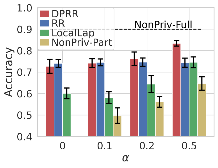
(c) Github StarGazers

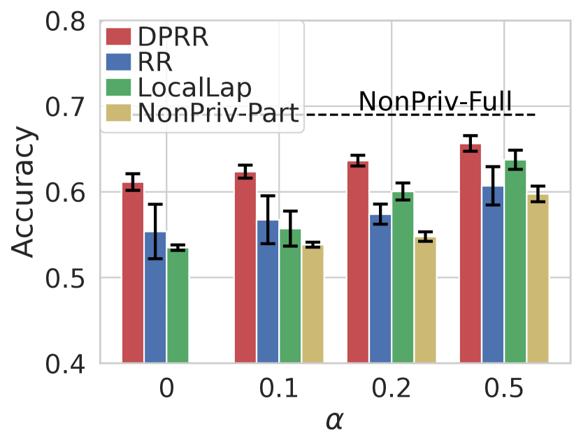
Figure 4: Classification accuracy and AUC for different $\alpha$ ($\varepsilon=1$). An error bar represents the standard deviation. Note that the RR is also inefficient in terms of the training/classification time and the memory size.

(a) REDDIT-MULTI-5K
(b) REDDIT-BINARY
(c) Github StarGazers
(a) REDDIT-MULTI-5K
(b) Github StarGazers

Figure 5: Classification accuracy and AUC for different $\varepsilon$ ($\alpha=0$). An error bar represents the standard deviation. Note that the RR is also inefficient in terms of the training/classification time and the memory size.

Figure 6: Classification accuracy for different budget allocation methods. An error bar represents the standard deviation.

We observe that our DPRR provides the best (or almost the best) performance in all cases. The DPRR significantly outperforms the RR in the customized setting where $\alpha>0$. The accuracy of the RR is hardly increased with an increase in $\alpha$. This is because the RR makes friend lists of private users dense. This ruins the neighborhood aggregation for non-private users. In contrast, the accuracy of our DPRR dramatically increases with an increase in $\alpha$. We also emphasize that the DPRR is much more efficient than the RR, as shown later.

We also observe that our DPRR significantly outperforms LocalLap in all cases. One reason for this is that LocalLap does not preserve each user’s degree information, as shown later. Our DPRR also significantly outperforms NonPriv-Part, which means that the DPRR effectively uses friend lists of private users.

Moreover, our DPRR provides accuracy close to NonPriv-Full with a reasonable privacy budget. For example, when $\varepsilon=1$ and $\alpha=0.2$, the difference in the classification accuracy or AUC is smaller than $0.1$ or so in all datasets. These results demonstrate the effectiveness of the DPRR.

In our experiments, the proportion $\alpha$ of non-private users is the same between training graphs and testing graphs. In practice, $\alpha$ can be different between them. However, we note that we can make $\alpha$ the same between training and testing graphs by adding DP noise for some non-private users. For example, assume that $\alpha=0.1$ in training graphs and $\alpha=0.2$ in testing graphs. By adding DP noise for some non-private users in the testing graphs, we can make $\alpha=0.1$ for both the training and testing graphs. Fig. 4 shows that our DPRR is effective for all values of $\alpha$ including $\alpha=0$.

Privacy Budget Allocation.  Next, we examined the effectiveness of our privacy budget allocation method in Section IV-D. Specifically, we compared our proposed method with the method that always sets $\varepsilon_{1}$ and $\varepsilon_{2}$ to $\varepsilon_{1}=\frac{\varepsilon}{10}$ and $\varepsilon_{2}=\frac{9\varepsilon}{10}$ ($\varepsilon_{1}:\varepsilon_{2}=1:9$). Here, we used REDDIT-MULTI-5K and Github StarGazers as datasets and set $\varepsilon=0.1$, $0.2$, $0.5$, or $1$.

Fig. 6 shows the results. “DPRR (Proposal)” represents our DPRR with our privacy budget allocation method. Note that “DPRR (Proposal)” is identical to “DPRR ($\varepsilon_{1}:\varepsilon_{2}=1:9$)” when $\varepsilon=0.5$ and $1$ (resp. $\varepsilon=1$) in REDDIT-MULTI-5K (resp. Github StarGazers). We observe that our privacy budget allocation method outperforms the baseline ($\varepsilon_{1}:\varepsilon_{2}=1:9$) when $\varepsilon$ is small. This is because our proposed method makes the Laplacian noise small. The difference is larger in Github StarGazers (see Fig. 7), because the original degree $d_{i}$ is smaller and is more susceptible to the Laplacian noise.

Degree Preservation.  We also examined how well the DPRR preserves each user’s degree information to explain the reason that the DPRR outperforms the RR and LocalLap. The left panels of Fig. 7 show the relationship between each user $v_{i}$’s original degree $d_{i}$ and noisy degree $\tilde{d}_{i}$. We also examined how the degree information of a graph correlates with its type. The right panels of Fig. 7 show a degree distribution (i.e., distribution of $d_{i}$) for each graph type.

(a) REDDIT-MULTI-5K
(b) REDDIT-BINARY
(c) Github StarGazers

Figure 7: Relationship between original degree $d_{i}$ and noisy degree $\tilde{d}_{i}$ (left) and degree distribution for each graph type (right) ($\varepsilon=1$). In the left panels, each point shows the result for one user.

The left panels of Fig. 7 show that the DPRR preserves the original degree very well. This holds especially when the original degree is small, e.g., $d_{i}<500$, $1000$, and $200$ in REDDIT-MULTI-5K, REDDIT-BINARY, and Github StarGazers, respectively. This is because the expectation of $\tilde{d}_{i}$ is almost equal to $d_{i}$ (see (11)) when $d_{i}\ll n$. In other words, the experimental results are consistent with our theoretical analysis. Moreover, the right panels of Fig. 7 show that $d_{i}<500$, $1000$, and $200$ in almost all cases in REDDIT-MULTI-5K, REDDIT-BINARY, and Github StarGazers, respectively. Thus, $\tilde{d}_{i}\approx d_{i}$ holds for the vast majority of users in the DPRR.

The right panels of Fig. 7 show that the degree information differs for each graph type. For example, in REDDIT-BINARY, the discussion-based community tends to have a larger degree than the question/answer-based community; i.e., the discussion-based community tends to attract more people.

The left panels of Fig. 7 show that the RR and LocalLap do not preserve the degree information for the vast majority of users. The RR makes neighbor lists of these users dense and destroys the graph structure. LocalLap makes neighbor lists sparse, irrespective of the original degrees. In contrast, the DPRR preserves the degree information for these users. This explains why the DPRR outperforms the RR and LocalLap.

Training/Classification Time.  Finally, we measured the time for training and classification on the server side in the DPRR, RR, and LocalLap. Here, we used two datasets: REDDIT-BINARY and a synthetic graph dataset based on the BA (Barabási-Albert) model [11]. The BA model is a graph generation model that has a power-law degree distribution. It generates a synthetic graph by adding new nodes one by one. Each node has $m\in\mathbb{N}$ new edges, and each edge is connected to an existing node with probability proportional to its degree. The average degree of the BA graph is $2m$. We used the NetworkX library [23] to generate the BA graph.

For each dataset, we evaluated the relationship between the training/classification time and the graph size. Specifically, in REDDIT-BINARY, we used $75\%$ of the graphs (i.e., $1500$ graphs) and $15\%$ of the graphs (i.e., $300$ graphs) for training and classification, respectively, as explained in Section V-A. For each graph, we randomly sampled $\gamma n$ nodes, where $\gamma\in[0,1]$ is a sampling rate, and used a subgraph composed of the sampled nodes. In the BA graph dataset, we generated $1000$ and $200$ graphs for training and classification, respectively. We set $m=3$ or $5$ and $n=1000$, $2000$, $3000$, or $4000$. We evaluated the relationship between the run time and $\gamma$ (resp. $n$) in REDDIT-BINARY (resp. BA graph dataset).

We measured the run time using a supercomputer in [1]. We used one computing node, which consists of two Intel Xeon Platium 8360Y processors (2.4 GHz, 36 Cores) and 512 GiB main memory. For training, we measured the time to run $100$ epochs because the training was stopped at $100$ to $200$ epochs in most cases, as described in Section V-A. For classification, we measured the time to classify all graphs for classification. We used the implementation in [3] as a code of GNN. Note that the DPRR, RR, and LocalLap only differ in the input to GNN, and therefore the comparison is fair.

Figure 8: Run time vs. sampling rate $\gamma$ in REDDIT-BINARY (left: training time, right: classification time).

(a) $m=3$
(b) $m=5$

Figure 9: Run time vs. #nodes $n$ in the BA graphs (left: training time, right: classification time).

Figs. 9 and 9 show the results. The run time of the RR is large and almost quadratic in the graph size, i.e., the sampling rate $\gamma$ in Fig. 9 and the number $n$ of nodes in Fig. 9. In contrast, the run time of the DPRR and LocalLap is much smaller than the RR. Fig. 9 shows that when the average degree is constant ($=2m$), the run time of the DPRR and LocalLap is almost linear in $n$. These results are consistent with Table II.

We can also estimate the run time for larger $n$ based on Fig. 8. For example, Fig. 8 (c) shows that when $m=5$ and $n=4000$, the training time of the RR and our DPRR is about $19000$ and $1500$ seconds, respectively. Thus, when $m=5$ and $n=40000$, the training time of the RR and our DPRR is estimated to be about $21$ days ($=19000\times 10^{2}$ seconds) and $4$ hours ($=1500\times 10/3600$ seconds), respectively. Therefore, our DPRR is much more efficient and practical than the RR.

Summary.  In summary, our answers to the three research questions at the beginning of Section V are as follows. [RQ1]: Our DPRR is much more efficient than the RR and provides higher accuracy than the RR, especially in the customized setting. Our DPRR also provides much higher accuracy than the other private baselines (LocalLap and NonPriv-Part) in terms of accuracy. [RQ2]: Our DPRR provides accuracy close to a non-private algorithm (NonPriv-Full) with a reasonable privacy budget, e.g., $\varepsilon=1$. [RQ3]: Our DPRR preserves each user’s degree information very well, whereas the RR and LocalLap do not. In addition, the degree information of a graph correlates with its type. These results explain why the DPRR outperforms the RR and LocalLap in terms of accuracy.

VI Conclusion

In this paper, we proposed the DPRR and a privacy budget allocation method to provide high accuracy in GNNs with a small privacy budget $\varepsilon$ in edge LDP. Through experimental evaluation, we showed that the DPRR outperforms the three baselines (RR, LocalLap, and NonPriv-Part) in terms of accuracy. We also showed that the DPRR is much more efficient than the RR in that it needs much less time for training and classification and much less memory.

Although we have focused on unattributed graphs, we can also provide LDP for both edges and feature vectors by combining our DPRR with the algorithm in [48]. Specifically, the authors in [48] propose an algorithm providing LDP for only feature vectors. They assume that original edges are public and use the original edges as input to their algorithms (Algorithms 2 and 3 in [48]). Here, we can use noisy edges output by our DPRR as input to their algorithms. In other words, we can combine our DPRR with the algorithms in [48] by replacing the original edges with the noisy edges output by our DPRR. Since the noisy edges provide LDP, we can provide LDP for both feature vectors and edges. We also note that although the algorithms in [48] focus on node classification, they can be easily applied to graph classification by using the mean readout as a graph pooling method, as in our experiments. For future work, we would like to evaluate the accuracy of the combined algorithms using attributed graphs.

Appendix A Proof of Proposition 2

Adding or removing one bit of $\mathbf{a}_{i}$ will change a degree $d_{i}$ of user $v_{i}$ by one. Thus, the global sensitivity of the degree is $1$, and adding $\textrm{Lap}(\frac{1}{\varepsilon_{1}})$ to $d_{i}$ (line 2 in Algorithm 2) provides $\varepsilon_{1}$-edge LDP. The subsequent sampling probability tuning (lines 4-5) is a post-processing on the noisy degree $d_{i}^{*}$ ($=d_{i}+\textrm{Lap}(\frac{1}{\varepsilon_{1}}))$. In addition, Warner’s RR with the flipping probability $1-p=\frac{1}{e^{\varepsilon_{2}}+1}$ (line 6) provides $\varepsilon_{2}$-edge LDP, as described in Section III-B. The subsequent edge sampling (line 7) is a post-processing on the noisy neighbor list $\tilde{\mathbf{a}}_{i}$.

Finally, we use the (general) sequential composition [36] of edge LDP, which is proved in [29]:

Lemma 1 (Sequential composition of edge LDP [29]).

For $i\in[n]$, let $\mathcal{R}\hskip 0.28453pt_{i}^{1}$ be a local randomizer of user $v_{i}$ that takes $\mathbf{a}_{i}\in\{0,1\}^{n}$ as input. Let $\mathcal{R}\hskip 0.28453pt_{i}^{2}$ be a local randomizer of $v_{i}$ that depends on the output $\mathcal{R}\hskip 0.28453pt_{i}^{1}(\mathbf{a}_{i})$ of $\mathcal{R}\hskip 0.28453pt_{i}^{1}$. If $\mathcal{R}\hskip 0.28453pt_{i}^{1}$ provides $\varepsilon_{1}$-edge LDP and for any $\mathcal{R}\hskip 0.28453pt_{i}^{1}(\mathbf{a}_{i})$, $\mathcal{R}\hskip 0.28453pt_{i}^{2}(\mathcal{R}\hskip 0.28453pt_{i}^{1}(\mathbf{a}_{i}))$ provides $\varepsilon_{2}$-edge LDP, then the sequential composition $(\mathcal{R}\hskip 0.28453pt_{i}^{1}(\mathbf{a}_{i}),\mathcal{R}\hskip 0.28453pt_{i}^{2}(\mathcal{R}\hskip 0.28453pt_{i}^{1}(\mathbf{a}_{i}))(\mathbf{a}_{i}))$ provides $(\varepsilon_{1}+\varepsilon_{2})$-edge LDP.

In our case, $\mathcal{R}\hskip 0.28453pt_{i}^{1}$ is the Laplacian mechanism followed by the sampling probability tuning, and $\mathcal{R}\hskip 0.28453pt_{i}^{2}$ is Warner’s RR followed by the edge sampling. $\mathcal{R}\hskip 0.28453pt_{i}^{2}$ depends on the output $q_{i}$ of $\mathcal{R}\hskip 0.28453pt_{i}^{1}$. Thus, by Lemma 1 (and the post-processing invariance), the DPRR provides $(\varepsilon_{1}+\varepsilon_{2})$-edge LDP. ∎

References

- [1] AI bridging cloud infrastructure (ABCI). https://abci.ai/, 2023.
- [2] The diaspora* project. https://diasporafoundation.org/, 2023.
- [3] How powerful are graph neural networks? https://github.com/weihua916/powerful-gnns, 2023.
- [4] Linkedin. https://www.linkedin.com/company/social-network, 2023.
- [5] Mastodon: Giving social networking back to you. https://joinmastodon.org/, 2023.
- [6] Reddit. https://www.reddit.com/, 2023.
- [7] Smule. https://www.smule.com/, 2023.
- [8] Tools: DPRR-GNN. https://github.com/DPRR-GNN/DPRR-GNN, 2023.
- [9] Jayadev Acharya, Kallista Bonawitz, Peter Kairouz, Daniel Ramage, and Ziteng Sun. Context-aware local differential privacy. In Proceedings of the 37th International Conference on Machine Learning (ICML’20), pages 52–62, 2020.
- [10] Jayadev Acharya, Ziteng Sun, and Huanyu Zhang. Hadamard response: Estimating distributions privately, efficiently, and with little communication. In Proceedings of the 22nd International Conference on Artificial Intelligence and Statistics (AISTATS’19), pages 1120–1129, 2019.
- [11] Albert-László Barabási. Network Science. Cambridge University Press, 2016.
- [12] Raef Bassily and Adam Smith. Local, private, efficient protocols for succinct histograms. In Proceedings of the 47th annual ACM Symposium on Theory of Computing (STOC’15), pages 127–135, 2015.
- [13] Suman K. Bera and C. Seshadhri. How to count triangles, without seeing the whole graph. In Proceedings of the 26th ACM SIGKDD International Conference on Knowledge Discovery & Data Mining (KDD’20), pages 306–316, 2020.
- [14] Rosalie Chan. The cambridge analytica whistleblower explains how the firm used facebook data to sway elections. https://www.businessinsider.com/cambridge-analytica-whistleblower-christopher-wylie-facebook-data-2019-10, 2019.
- [15] Zhengdao Chen, Lisha Li, and Joan Bruna. Supervised community detection with line graph neural networks. In Proceedings of the 7th International Conference on Learning Representations (ICLR’19), pages 1–24, 2019.
- [16] Ben Coleman. Releasing counts with differential privacy. https://randorithms.com/2020/10/09/geometric-mechanism.html, 2020.
- [17] Bolin Ding, Janardhan Kulkarni, and Sergey Yekhanin. Collecting telemetry data privately. In Proceedings of the 31st Conference on Neural Information Processing Systems (NIPS’17), pages 3574–3583, 2017.
- [18] Cynthia Dwork and Aaron Roth. The Algorithmic Foundations of Differential Privacy. Now Publishers, 2014.
- [19] Talya Eden, Amit Levi, Dana Ron, and C. Seshadhri. Approximately counting triangles in sublinear time. In Proceedings of the 2015 IEEE 56th Annual Symposium on Foundations of Computer Science (FOCS’15), pages 614–633, 2015.
- [20] Ulfar Erlingsson, Vasyl Pihur, and Aleksandra Korolova. RAPPOR: Randomized aggregatable privacy-preserving ordinal response. In Proceedings of the 2014 ACM SIGSAC Conference on Computer and Communications Security (CCS’14), pages 1054–1067, 2014.
- [21] Federico Errica, Marco Podda, Davide Bacciu, and Alessio Micheli. A fair comparison of graph neural networks for graph classification. In Proceedings of the 8th International Conference on Learning Representations (ICLR’20), pages 1–16, 2020.
- [22] Justin Gilmer, Samuel S. Schoenholz, Patrick F. Riley, Oriol Vinyals, and George E. Dahl. Neural message passing for quantum chemistry. In Proceedings of the 34th International Conference on Machine Learning (ICML’17), pages 1263–1272, 2017.
- [23] Aric A. Hagberg, Daniel A. Schult, and Pieter J. Swart. Exploring network structure, dynamics, and function using networkx. In Proceedings of the 7th Python in Science Conference (SciPy’08), pages 11–15, 2008.
- [24] William L. Hamilton, Rex Ying, and Jure Leskovec. Inductive representation learning on large graphs. In Proceedings of the 31st Conference on Neural Information Processing Systems (NIPS’17), pages 1024–1034, 2017.
- [25] Kaveh Hassani. Cross-domain few-shot graph classification. In Proceedings of the 36th AAAI Conference on Artificial Intelligence (AAAI’22), 2022.
- [26] Xinlei He, Jinyuan Jia, Michael Backes, Neil Zhenqiang Gong, and Yang Zhang. Stealing links from graph neural networks. In Proceedings of the 30th Usenix Security Symposium (Usenix Security’21), pages 2669–2686, 2021.
- [27] Nobuaki Hoshino. A firm foundation for statistical disclosure control. Japanese Journal of Statistics and Data Science, 3:721–746, 2020.
- [28] Jacob Imola, Takao Murakami, and Kamalika Chaudhuri. Locally differentially private analysis of graph statistics. In Proceedings of the 30th USENIX Security Symposium (USENIX Security’21), pages 983–1000, 2021.
- [29] Jacob Imola, Takao Murakami, and Kamalika Chaudhuri. Communication-efficient triangle counting under local differential privacy. In Proceedings of the 31th USENIX Security Symposium (USENIX Security’22), 2022.
- [30] Xun Jian, Yue Wang, and Lei Chen. Publishing graphs under node differential privacy. IEEE Transactions on Knowledge and Data Engineering, 35(4):4164–4177, 2023.
- [31] Hongwei Jin and Xun Chen. Gromov-wasserstein discrepancy with local differential privacy for distributed structural raphs. CoRR, 2202.00808, 2022.
- [32] Dave Johnson. How to hide your friends list on facebook, from everyone or only certain people. https://www.businessinsider.com/how-to-hide-friends-on-facebook, 2019.
- [33] Zach Jorgensen, Ting Yu, and Graham Cormode. Conservative or liberal? Personalized differential privacy. In Proceedings of IEEE 31st International Conference on Data Engineering (ICDE’15), pages 1023–1034, 2015.
- [34] Peter Kairouz, H. Brendan McMahan, and Brendan Avent et al. Advances and open problems in federated learning. Foundations and Trends in Machine Learning, 14(1-2):1–210, 2021.
- [35] Thomas N. Kipf and Max Welling. Semi-supervised classification with graph convolutional networks. In Proceedings of the 5th International Conference on Learning Representations (ICLR’17), pages 1–14, 2017.
- [36] Ninghui Li, Min Lyu, and Dong Su. Differential Privacy: From Theory to Practice. Morgan & Claypool Publishers, 2016.
- [37] Wanyu Lin, Baochun Li, and Cong Wang. Towards private learning on decentralized graphs with local differential privacy. IEEE Transactions on Information Forensics and Security, 17:2936–2946, 2022.
- [38] Yao Ma and Jiliang Tang. Deep Learning on Graphs. Cambridge University Press, 2021.
- [39] Chris Morris. The number of data breaches in 2021 has already surpassed last year’s total. https://fortune.com/2021/10/06/data-breach-2021-2020-total-hacks/, 2021.
- [40] Tamara T. Mueller, Johannes C. Paetzold, Chinmay Prabhakar, Dmitrii Usynin, Daniel Rueckert, and Georgios Kaissis. Differentially private graph classification with GNNs. CoRR, 2202.02575, 2022.
- [41] Hiep H. Nguyen, Abdessamad Imine, and Michaël Rusinowitch. Network structure release under differential privacy. Transactions on Data Privacy, 9(3):215–214, 2016.
- [42] Iyiola E. Olatunji, Thorben Funke, and Megha Khosla. Releasing graph neural networks with differential privacy guarantees. CoRR, 2109.08907, 2021.
- [43] Thomas Paul, Antonino Famulari, and Thorsten Strufe. A survey on decentralized online social networks. Computer Networks, 75:437–452, 2014.
- [44] Zhan Qin, Yin Yang, Ting Yu, Issa Khalil, Xiaokui Xiao, and Kui Ren. Heavy hitter estimation over set-valued data with local differential privacy. In Proceedings of the 2016 ACM SIGSAC Conference on Computer and Communications Security (CCS’16), pages 192–203, 2016.
- [45] Zhan Qin, Ting Yu, Yin Yang, Issa Khalil, Xiaokui Xiao, and Kui Ren. Generating synthetic decentralized social graphs with local differential privacy. In Proceedings of the 2017 ACM SIGSAC Conference on Computer and Communications Security (CCS’17), pages 425–438, 2017.
- [46] Sofya Raskhodnikova and Adam Smith. Differentially Private Analysis of Graphs, pages 543–547. Springer, 2016.
- [47] Benedek Rozemberczki, Oliver Kiss, and Rik Sarkar. Karate club: An api oriented open-source python framework for unsupervised learning on graphs. In Proceedings of the 29th ACM International Conference on Information and Knowledge Management (CIKM’20), page 3125–3132, 2020.
- [48] Sina Sajadmanesh and Daniel Gatica-Perez. Locally private graph neural networks. In Proceedings of the 2021 ACM SIGSAC Conference on Computer and Communications Security (CCS’21), pages 2130–2145, 2021.
- [49] Sina Sajadmanesh, Ali Shahin Shamsabadi, Aurélien Bellet, and Daniel Gatica-Perez. GAP: Differentially private graph neural networks with aggregation perturbation. In Proceedings of the 32nd USENIX Security Symposium (USENIX Security’23), 2023.
- [50] Comandur Seshadhri, Tamara G. Kolda, and Ali Pinar. Community structure and scale-free collections of erdös-rényi graphs. Physical Review E, 85(5):1–9, 2012.
- [51] Reza Shokri and Vitaly Shmatikov. Privacy-preserving deep learning. In Proceedings of the 22nd ACM SIGSAC Conference on Computer and Communications Security (CCS’15), pages 1310–1321, 2015.
- [52] Tianhao Wang, Jeremiah Blocki, Ninghui Li, and Somesh Jha. Locally differentially private protocols for frequency estimation. In Proceedings of the 26th USENIX Security Symposium (USENIX Security’17), pages 729–745, 2017.
- [53] Stanley L. Warner. Randomized response: A survey technique for eliminating evasive answer bias. Journal of the American Statistical Association, 60(309):63–69, 1965.
- [54] Bin Wu, Ke Yi, and Zhenguo Li. Counting triangles in large graphs by random sampling. IEEE Transactions on Knowledge and Data Engineering, 28(8):2013–2026, 2016.
- [55] Chuhan Wu, Fangzhao Wu, Yang Cao, Yongfeng Huang, and Xing Xie. FedGNN: Federated graph neural network for privacy-preserving recommendation. CoRR, 2102.04925, 2021.
- [56] Fan Wu, Yunhui Long, Ce Zhang, and Bo Li. LinkTeller: Recovering private edges from graph neural networks via influence analysis. In Proceedings of the 2022 IEEE Symposium on Security and Privacy (S&P’22), pages 522–541, 2022.
- [57] Zonghan Wu, Shirui Pan, Fengwen Chen, Guodong Long, Chengqi Zhang, and Philip S. Yu. A comprehensive survey on graph neural networks. CoRR, 1901.00596, 2019.
- [58] Keyulu Xu, Weihua Hu, Jure Leskovec, and Stefanie Jegelka. How powerful are graph neural networks? In Proceedings of the 7th International Conference on Learning Representations (ICLR’19), pages 1–17, 2019.
- [59] Pinar Yanardag and S.V.N. Vishwanathan. Deep graph kernels. In Proceedings of the 21th ACM SIGKDD International Conference on Knowledge Discovery and Data Mining (KDD’15), pages 1365–1374, 2015.
- [60] Jaewon Yang and Jure Leskovec. Defining and evaluating network communities based on ground-truth. In Proceedings of the 2012 Ninth IEEE International Conference on Data Mining (ICDM’12), pages 745–754, 2012.
- [61] Qingqing Ye, Haibo Hu, Man Ho Au, Xiaofeng Meng, and Xiaokui Xiao. LF-GDPR: A framework for estimating graph metrics with local differential privacy. IEEE Transactions on Knowledge and Data Engineering (Early Access), pages 1–16, 2021.
- [62] Jiaxin Ying, Jiaqi Ma, and Qiaozhu Mei. A simple yet effective method improving graph fingerprints for graph-level prediction. In Proceedings of the 2021 Workshop on Graph Learning Benchmarks (GLB’21), pages 1–9, 2021.
- [63] Rex Ying, Jiaxuan You, Christopher Morris, Xiang Ren, William L. Hamilton, and Jure Leskovec. Hierarchical graph representation learning with differentiable pooling. In Proceedings of the 32nd International Conference on Neural Information Processing Systems (NIPS’18), pages 4805–4815, 2018.
- [64] Quan Yuan, Zhikun Zhang, Linkang Du, Min Chen, Peng Cheng, and Mingyang Sun. PrivGraph: Differentially private graph data publication by exploiting community information. In Proceedings of the 32nd USENIX Security Symposium (USENIX Security’23), 2023.
- [65] Zaixi Zhang, Qi Liu, Zhenya Huang, Hao Wang, Chengqiang Lu, Chuanren Liu, and Enhong Chen. GraphMI: Extracting private graph data from graph neural networks. In Proceedings of the 30th International Joint Conference on Artificial Intelligence (IJCAI’21), pages 3749–3755, 2021.
- [66] Zhikun Zhang, Min Chen, Michael Backes, Yun Shen, and Yang Zhang. Inference attacks against graph neural networks. In Proceedings of the 31th USENIX Security Symposium (USENIX Security’22), 2022.